Detection of PIT-Tagged Juvenile Salmonids in the Columbia River Estuary using a Pair-Trawl, 2011

Matthew S. Morris, Robert J. Magie, Benjamin P. Sandford, Jeremy P. Bender,

Amy L. Cook, and Richard D. Ledgerwood

Report of research by

Fish Ecology Division Northwest Fisheries Science Center National Marine Fisheries Service

National Oceanic and Atmospheric Administration 2725 Montlake Boulevard East

Seattle, Washington 98112-2097

for

Division of Fish and Wildlife

Bonneville Power Administration U.S. Department of Energy

P.O. Box 3621 Portland, Oregon 97208

Contract 46273 Rel 3 Project 199302900

September 2012

ii

iii

EXECUTIVE SUMMARY In 2011, we continued a study to detect juvenile anadromous salmonids Oncorhynchus spp. implanted with passive integrated transponder (PIT) tags using a surface pair-trawl fitted with a PIT-tag detection system. We sampled along the navigation channel in the upper Columbia River estuary between river kilometers (rkm) 61 and 83 for 671 h between 22 March and 1 July and detected a total of 14,123 PIT-tagged juvenile salmonids. These detections were comprised of 15% wild and 78% hatchery-reared fish (7% were of unknown origin). Of all PIT-tagged fish detected in the trawl during 2011, 40% were spring/summer Chinook salmon, 12% were fall Chinook salmon, 38% were steelhead, 3% were sockeye, 2% were coho, and 4% were unknown species. In 2011, sampling was conducted almost exclusively with our "matrix" PIT-tag detection system. This system was composed of a 122-m-long surface pair-trawl that funneled fish through a 2.6-m wide by 3.0-m tall fish-passage opening. The fish-passage structure was constructed with separate front and rear components, with each component consisting of 3 parallel antennas (for a total of six detection antennas) controlled by a single multiplexing transceiver. We maintained a distance of 91.5 m between the forward sections of the trawl wings while the trawl sampled from the surface to a depth of about 5.0 m. High flows through most of the migration season in 2011 had a substantial impact on fish facility operations at dams throughout the basin, and contributed to much lower detection numbers during trawl sampling as well (14,123 detections in 2011 compared to 31,327 in 2010). Higher flows increase fish migration speed to the estuary and disperse migrants across a greater volume of water in the sample reach, resulting in lower detection rates. High flows also reduced sample time, as crews were required to travel further up the sample reach to set the net, and time to remain within the sample reach during deployment was shorter. The larger fish-passage corridor of the matrix antenna, used since 2008, allowed most debris to pass through the trawl, and little sample time was lost due to the unusually high amounts of debris associated with high flows. The high debris loads at dams also required periodic removal of traveling fish screens, temporarily halted fish transportation, and in general lowered PIT-tag detection rates at fish facilities. We sampled during the spring migration period targeting the 607,504 yearling Chinook salmon and 300,454 juvenile steelhead PIT-tagged and released into the Snake River (PTAGIS; PSMFC 2011). Some of these fish were diverted for transportation at Lower Granite, Little Goose, Lower Monumental, and McNary Dams; a total of 209,799

iv

PIT-tagged fish were transported. Transported fish were generally released about 5 km downstream from Bonneville Dam, the lowermost dam on the Columbia River, and about 140 km upstream from our sample site. Coinciding with the anticipated arrival of early migrating juvenile PIT-tagged salmon and steelhead in the estuary, we began sampling on 22 March with a single daily shift operating 3-5 d week-1. As numbers of migrating juvenile salmonids in the estuary increased, we increased our sampling effort to two daily shifts operating 7 d week-1. Intensive sampling began on 2 May and continued through 10 June, after which we resumed operating with a single daily shift. Sampling ended on 1 July as numbers of PIT-tagged fish in the sampling reach declined. During the intensive sampling period, the trawl was deployed for an average of 12 h/d and we detected 1.8% of the inriver migrant yearling Chinook and 2.8% of the inriver migrant steelhead previously detected at Bonneville Dam. By comparison, during intensive sampling in 2010, the trawl was deployed for an average of 13 h/d and detected 3.7% of the yearling Chinook and 4.1% of the steelhead detected at Bonneville Dam. Likewise, we detected 1.2% of transported yearling Chinook salmon in 2011 vs. 3.0% in 2010, and 2.6% of transported steelhead in 2011 vs. 3.0% in 2010. In 2011, 19% of the PIT-tagged fish we detected had been transported and 6% had been detected at Bonneville Dam. The remaining 75% had not been transported or detected at Bonneville Dam, and the majority of these had passed Bonneville Dam undetected via spillway or turbine routes. The lower detection rate of fish previously detected at Bonneville Dam (6% in 2011 vs. 22% in 2010) was partially due to the removal of fish guidance screens during much of the migration season. These screens are used to divert fish from turbines and into the juvenile fish facility and subsequent PIT-tag detection arrays. Detection capability of the corner collector at Bonneville Dam remained active all season. Diel detection rates were similar between wild and hatchery rearing types for both yearling Chinook salmon and steelhead; thus we pooled data among rearing types for statistical analyses of diel trends. During the two-shift sampling period, we averaged 11 detections h-1 during daylight and 15 h-1 during darkness for yearling Chinook salmon (P = 0.041). During the same period for steelhead the trend was opposite, with 14 detections h-1 during daylight and 4 detections h-1 during darkness (P = 0.003). Survival estimates for fish migrating from Lower Granite Dam to the tailrace of Bonneville Dam were lower in 2011 than in 2010 for both yearling Chinook salmon (51.3 vs. 56.9%) and steelhead (60.0 vs. 60.8%). Detections of sockeye were insufficient for a reliable estimate of survival. Survival from McNary Dam to Bonneville Dam for both

v

Snake River and Upper-Columbia River yearling Chinook salmon was also lower in 2011 (68.7 and 58.4%) than in 2010 (73.8 vs. 73.5%). Survival from McNary to Bonneville Dam was higher in 2011 than in 2010 for steelhead from both the Snake (86.6 vs. 78.9%) and Upper-Columbia River (66.8 vs. 62.6%). Seasonal mean travel speed to Jones Beach was significantly faster for yearling Chinook salmon detected passing Bonneville Dam (91 km d-1) than for those released from barges just below the dam (75 km d-1; P ≤ 0.001). There was also a significant difference in travel speed between steelhead detected at Bonneville (102 km d-1) and barged steelhead (94 km d-1; P ≤ 0.001). Unlike yearling Chinook salmon, travel speed to the estuary was not significantly different for subyearling fall Chinook salmon detected at Bonneville Dam (mean 86 km d-1) than for those released from barges (mean 84 km d-1) during the same period (P = 0.685). We detected 1,098 subyearling fall Chinook salmon in 2011, with most detected after the intensive sample period. Of the total, 1,054 had originated in the Snake River basin (774 detected at Bonneville and 280 transported). The remaining 44 subyearling fish were Columbia River stocks. We also detected 18 fall Chinook salmon from the Snake River basin that had been released as subyearlings in 2010 but had overwintered in either the Snake or Columbia River and migrated through the estuary in 2011. In 2011, we detected 434 sockeye salmon; 78% had been released into the Snake River and 22% into the Columbia River. Of these fish, 93% were hatchery reared, <1% were wild, and the remaining 7% were of unknown origin. Fish detected at Bonneville Dam made up 79% of the total sockeye detections (341), while the remaining 21% were fish that had been transported (93). A prototype mobile separation by code system (MSbyC) was initially tested in 2010. Modifications over the following winter were made to improve passage through the system and minimize impacts to fish health. A single 2.3-h deployment of the improved MSbyC system was conducted on 24 June 2011 to assess these modifications. For this deployment, the system was attached to a normal-sized trawl. Fish passage appeared to be improved and impacts to fish reduced compared with tests in 2010. However, delays in fabrication precluded conclusive testing of impacts to fish. We diverted 4 PIT-tagged fish to the MSbyC sample tank and recorded data for fish with known migration history. Mean growth rate since tagging for these 4 fish was 0.33 m d-1 (range 0.24-0.43 mm d-1). We also sampled all fish (tagged and non-tagged) collected by the trawl with the MSbyC diversion gate locked in the open position. During two tests with a total sample time of 2.5 minutes, we collected 92 non-tagged Chinook salmon and 2 steelhead.

vi

vii

CONTENTS EXECUTIVE SUMMARY ............................................................................................... iii INTRODUCTION .............................................................................................................. 1 MATRIX ANTENNA TRAWL SYSTEM ........................................................................ 3

Methods................................................................................................................... 3 Study Area .................................................................................................. 3 Study Fish ................................................................................................... 4 Sample Period ............................................................................................. 5 Trawl System Design .................................................................................. 5 Electronic Equipment and Operation .......................................................... 7 Impacts on Fish ........................................................................................... 7

Results and Discussion ........................................................................................... 8 Detection Totals and Species Composition ................................................ 8 Impacts on Fish ......................................................................................... 13

ANALYSES FROM TRAWL DETECTION DATA....................................................... 15

Diel Detection Patterns ......................................................................................... 15 Methods..................................................................................................... 15 Results and Discussion ............................................................................. 15

Survival during Downstream Migration ............................................................... 18 Methods..................................................................................................... 18 Results and Discussion ............................................................................. 18

Travel Time of Transported vs. Inriver Migrant Fish ........................................... 23 Methods..................................................................................................... 23 Results and Discussion ............................................................................. 23

Yearling Chinook Salmon and Steelhead ..................................... 23 Subyearling Fall Chinook Salmon ................................................ 27 Subyearling Fall Chinook Salmon ................................................ 29

Detection Rates of Transported vs. Inriver Migrant Fish ..................................... 31 Methods..................................................................................................... 31 Results and Discussion ............................................................................. 32

DEVELOPMENT OF A MOBILE SEPARATION-BY-CODE SYSTEM ..................... 37

Methods................................................................................................................. 37 Results and Discussion ......................................................................................... 39

REFERENCES ................................................................................................................. 43 APPENDIX A: Data Tables............................................................................................. 47 APPENDIX B: Detection Efficiency Tests ..................................................................... 63

viii

INTRODUCTION In 2011, we continued a multi-year study in the Columbia River estuary to collect data on migrating juvenile Pacific salmon Oncorhynchus spp. implanted with passive integrated transponder (PIT) tags (Ledgerwood et al. 2004; Magie et al. 2011). Data from estuary detections are used to estimate the survival and downstream migration timing of these fish. As in previous years, we used a large surface pair-trawl to guide fish through an array of detection antennas mounted in place of the cod-end of the trawl. Target fish were PIT-tagged for various research projects at natal streams, hatcheries, collector dams, and other upstream locations (PSMFC 2011). When PIT-tagged fish passed through the trawl and antennas, their tag code, GPS position and date and time were electronically recorded. This study began in 1995 and has continued annually (except 1997) in the estuary near Jones Beach, approximately 75 river kilometers (rkm) upstream from the mouth of the Columbia River. More than 2.5 million Snake and Columbia River juvenile salmonids were PIT-tagged and released in the basin either prior to or during the spring migration of 2011 (PSMFC 2011). During migration, a portion of these fish were monitored at dams equipped with PIT-tag detection systems (Prentice et al. 1990a,b,c). These systems automatically upload detection information to the PIT Tag Information System database (PTAGIS), a regional database that stores and disseminates information on PIT-tagged fish (PSMFC 2011). Consistent with other interrogation sites, we uploaded our detection records to PTAGIS and downloaded information on the fish we detected with the trawl system. Data recorded in PTAGIS includes the species, origin (wild or hatchery) release location, date and time and detection history of individual fish. We have used detections from the estuary pair trawl to evaluate migration timing between Bonneville Dam and the estuary for transported fish and to evaluate survival and migration timing of yearling Chinook salmon and steelhead migrating through the entire hydrosystem each year since 1998. Detection data in 2011 was sufficient to conduct these comparisons for juvenile Chinook salmon O. tshawytscha and steelhead O. mykiss. In 2011, over 200,000 PIT-tagged fish were transported from dams on the Snake or Columbia River and over 60,000 were detected at Bonneville Dam. Seasonal trends in these data may provide insight into the variation observed in smolt-to-adult return (SAR) ratios of NMFS transportation study fish, which has been shown to relate to juvenile migration timing (Marsh et al. 2008, 2012).

2

3

MATRIX ANTENNA TRAWL SYSTEM

Methods Study Area Trawl sampling was conducted in the upper Columbia River estuary between Eagle Cliff (rkm 83) and the west end of Puget Island (rkm 61; Figure 1). This is a freshwater reach characterized by frequent ship traffic, occasional severe weather, and river currents often exceeding 1.1 m s-1. Tides in this area are semi-diurnal, with about 7 h of ebb and 4.5 h of flood. During the spring freshet (April-June), little or no flow reversal occurs in this reach during flood tide, especially in years of medium-to-high river flow. The trawl was deployed adjacent to a 200-m-wide navigation channel, which is maintained at a depth of 14 m. Figure 1. Trawling area adjacent to the navigation channel in the upper Columbia River

estuary between rkm 61 and 83.

4

Study Fish We continued to focus detection efforts on large release-groups of PIT-tagged fish, particularly those detected at Bonneville Dam and those transported and released just downstream from the dam. The vast majority of these fish enter the upper estuary from late April through late June. Release dates and locations of fish detected with the trawl were retrieved from the PTAGIS database (PSFMC 2011). These included approximately 785,0001 fish released for NMFS transportation studies and nearly 208,000 fish released for a comparative survival study of hatchery fish, as well as smaller groups released for other studies. Of the PIT-tagged fish released in the Columbia River basin for migration in 2011, 209,799 were collected at dams and diverted for transportation and release below Bonneville Dam. We coordinated trawl system operations with the expected passage timing of fish tagged and released for NMFS transportation studies. After being tagged at Lower Granite Dam (rkm 695), transportation study fish were either loaded to transport barges, released to migrate in the river, or collected and transported from dams downstream from the release site. Dams with transport facilities included Lower Granite, Little Goose (rkm 635), Lower Monumental (rkm 589), and McNary Dam (rkm 470). Our analysis included all transported fish detected in the trawl, regardless of the location from which they were transported. To track fish recorded as having been diverted, or possibly diverted, for transportation at any of the four transport dams, we created an independent database (Microsoft Access) using data downloaded from PTAGIS. At the transport dams, PIT-tagged fish were diverted using separation-by-code (SbyC) systems (Stein et al. 2004). Diversion to a transport barge was verified for PIT-tagged fish last detected at a dam on a route that ended at a transport raceway, according to monitor locations on the PTAGIS site map. Some fish had tag codes that indicated the fish was pre-designated for SbyC transport, but there was no detection record on a transport raceway to confirm barge loading. These records were excluded from our transportation analysis, as were fish removed for biological or other samples. Since 1987, we have collectively recorded data from nearly 3 million transported PIT-tagged fish. The U.S. Army Corps of Engineers (John Bailey, personal communication) provided individual barge-loading dates and times for each dam throughout the 2011 transportation season. By comparing barge loading times with the

1 Total includes 571,864 subyearlings released with transport beginning in mid-May

5

last detection time of fish diverted to transport raceways, we determined the individual barge-transport trip for each fish. With this information, we were able to derive the specific date, time, and release location of each individual transported fish. Travel time and relative survival to the estuary for these fish was compared with that of fish detected at Bonneville Dam. We modified the PTAGIS information in our local database to include these migration history data. We then created paired comparison groups of transported fish released from barges and fish detected at Bonneville Dam on the same date. In addition to the transportation study, several other studies in the Columbia River Basin released large numbers of spring-migrating, PIT-tagged juvenile salmonids. Sufficient numbers of fish for timing and survival analyses were obtained from the more numerous yearling Chinook salmon and steelhead. Sockeye and subyearling Chinook salmon detections allowed for some analyses, but these were limited due to the smaller sample sizes and later run timing. We also recorded detections of PIT-tagged coho salmon O. kisutch and coastal cutthroat trout O. clarki clarki. Sample Period Spring and summer sampling with the matrix antenna trawl system began on 22 March and continued through 1 July 2011. Because the availability of fish in the estuary varied, our sample effort varied accordingly and was not equal during all days within this period. At the beginning and end of the migration season, we sampled with a single shift, 2-5 d week-1 for an average daily effort of about 5 h d-1. From 2 May through 10 June, we sampled with two shifts daily (7 day shifts and 6 night shifts weekly) for an average daily effort of 12 h d-1. During the two-shift period, day shifts began before dawn and continued for 6-10 h, while night shifts began in late afternoon and continued through most of the night or until relieved by the day crew. Sampling was intended to be nearly continuous throughout the two-shift period except between 1400 and 1900 PDT, when we interrupted sampling for fueling and maintenance. In 2011, sampling did not occur during one swing shift per week. Trawl System Design In 2011, sampling was conducted almost exclusively with the matrix-antenna trawl system (Figure 2). The fish passage corridor was configured with three parallel coils in front and three in the rear, for a total of six detection coils. Inside dimensions of individual coils measured 0.75 by 2.8 m. Front and rear components were connected by a 1.5-m length of net mesh, and the overall fish-passage opening was 2.6 by 3.0 m. The

6

matrix antenna was attached at the rear of the trawl and suspended by buoys 0.6 m beneath the surface. This configuration allowed fish collected in the trawl to exit through the antenna while remaining in the river. Each 3-coil component of the matrix antenna weighed approximately 114 kg in air and required an additional 114 kg of lead weight to sink in the water column (total weight of both components was 456 kg in air). The trawl with attached antenna was transported to/from the sample area aboard one net-reel tow vessel. Figure 2. Basic design of the surface pair trawl used with the matrix antenna system to

sample juvenile salmonids in the Columbia River estuary (rkm 75), 2011. The basic configuration of the pair-trawl net has changed little through the years, despite changes to the PIT-tag detection apparatus (Ledgerwood et al. 2004). The upstream end of each wing of the trawl initiated with a 3-m-long spreader bar shackled to the wing section. The end of each wing was attached to the 30.5-m-long trawl body, which was modified for antenna attachment. The mouth of the trawl body had an opening 9 m wide by 6 m tall with a 6.1 m floor extending forward from the mouth. Sample depth was about 4.6 m due to curvature in the side-walls under tow.

7

We towed the net with two 73-m-long tow lines to prevent turbulence on the net from the two tow vessels. After the trawl and antenna were deployed, one tow line was passed to an adjacent tow vessel (pair-trawling). During a typical deployment, the net was towed upstream facing into the current, with a distance of about 91.5 m between the trawl wings. Even though volitional passage through the trawl and antenna occurred while towing with the wings extended, we continued to bring the wings of the trawl together every 17 minutes to flush debris out of the system. The majority of fish were detected during these 7-minute net-flushing periods. Electronic Equipment and Operation We used the same electronic components and procedures as in 2006-2010. We used a single Digital Angel model FS1001M multiplexing transceiver, which was capable of simultaneously powering, recording, and transmitting data for up to six antenna detection coils. Electronic components for the trawl system were contained in a water-tight box (0.8 × 0.5 × 0.3 m) mounted on a 2.4 by 1.5-m pontoon raft tethered behind the antenna. Data were transmitted from each antenna coil to specific transceiver ports via armored cable. The system used a DC power source for the transceiver and antenna. Data were then wirelessly transmitted and recorded to a computer onboard a tow vessel. Detection efficiency tests were conducted to verify performance of the system (Appendix B). The date and time of detection, tag code, coil identification number, and GPS location for each fish detected were received from the antenna and recorded automatically using the computer software program MiniMon (PSMFC 2011). Written logs were maintained for each sampling cruise noting the time and duration of net deployment, net retrieval, approximate location, and any incidence of impinged fish. Detection data files were uploaded periodically (about weekly) to PTAGIS using standard methods described in the PIT-tag Specification Document (Stein et al. 2004). The specification document, PTAGIS operating software, and user manuals are available via the internet (PSMFC 2011). Pair-trawl detections are designated in the PTAGIS database with site code TWX (towed array-experimental). Impacts on Fish We used visual observation and periodic deployment of underwater video cameras to inspect the cod-end of the net for debris accumulation near the antenna that could impact fish. Other sections of the net were monitored visually from a skiff, and accumulated debris was removed from net sections as necessary. During retrieval, the matrix antenna was hoisted on to a tow vessel while remaining attached to the pair trawl. This retrieval method saved time and was possible due to the larger fish-passage opening

8

of the matrix antenna. Previous antenna designs, such as the cylindrical antenna (0.9-m diameter) last used in 2009, allowed significant accumulations of debris in the trawl body. Thus the trawl had to be inverted for debris removal during each retrieval, and this required the antenna to be disconnected from the trawl (Magie et al. 2010). In contrast, the matrix antenna design allowed most debris to pass through the system, resulting in an overall reduction of debris accumulation. Debris that remained in the net was removed by hand through zippers in the top of the trawl body. During debris-removal activities, we recorded all impinged or trapped fish as mortalities, even if they were released alive.

Results and Discussion Detection Totals and Species Composition Sampling through most of the intensive (two daily shifts) sampling period in 2011 was characterized by high river flows and heavier-than-normal debris loads. Mean flow volumes in the Columbia River at Bonneville Dam were about 72% higher during the two-shift sample period of 2011 (11,800 m3 s-1) than during the two-shift period of 2010 (6,841 m3 s-1; Figure 3). We estimate that our intensive sampling period in 2011 coincided with the arrival in the estuary of over 65% of the fish passing Bonneville Dam (tagged and non-tagged) and 73% of the transported fish from NMFS transportation studies (tagged and non-tagged). In contrast, we estimated that intensive sampling in 2011 coincided with 89% of fish passing Bonneville and 83% of transported fish. The proportion of PIT-tagged fish detected at Bonneville Dam was unusually low in 2011 (71% lower than in 2010) because the fish guidance screens used to divert fish from turbine intakes into the juvenile fish bypass facility were removed during the height of the migration season due to heavy debris accumulation. At present, only fish guided into the juvenile facility or those passing via the corner collector (a surface flow bypass system), can be interrogated for PIT-tags at Bonneville Dam. Juvenile migrants that are diverted to the fish facility (tagged or non-tagged) may be collected for biological samples, but the majority are returned to the river via the tailrace of the dam. Fish guidance screens at Bonneville were removed on 24 May and remained out of service through 1 July. Fish detected at the dam while guidance screens were removed had either entered the juvenile facility volitionally or had passed via the corner collector.

9

12,000

9,000

6,000

3,000

029 Apr 6 May 13 May 20 May 27 May 3 Jun 10 Jun

2010avg 98-09, no 20012001 2011Fl

ow (m

3 s-1

)15,000

Figure 3. Columbia River flows at Bonneville Dam during the two-shift sample periods

in 2010 and 2011, as compared to the average flow from 1998 to 2009 (excluding 2001). Drought-year flows for 2001 are also shown for comparison.

Four barge releases of yearling Chinook salmon and steelhead occurred prior to the beginning of our intensive sampling period. Very few inriver migrant fish from the transportation study were detected prior to the intensive sampling period as well, although these fish would not be expected in the estuary for several days or weeks after the release of transported fish. After the intensive sampling period had ended, most fish detected at Bonneville Dam were subyearling Chinook salmon, which continue to migrate into the summer months. Subyearlings were transported and released into October. We sampled with the matrix trawl system for 671 h during 2011 and detected 14,123 PIT-tagged fish. By comparison, in 2010 we sampled for 902 h and detected 31,327 fish (Figure 4). Detection rates in 2011 were lower than in 2010 (21 vs. 35 fish h-1), even though a similar number of PIT-tagged fish was released during the spring migration in both years. Since pair-trawl sampling began in 1998, we have observed a strong relationship between flow and detection rates, with increasing river flows associated with decreasing detection rates of fish previously detected at Bonneville Dam (a rough measure of sample efficiency; Magie et al. 2010, 2011).

10

Spring and Summer Daily Detection Effort

2010

24

18

12

Two-Crew mean 12 hours per day (2 May – 10 June)

2011

6

Detections: 14,123Total Hours: 671

Sam

ple

Effo

rt (h

)

15 Mar 14 Apr 14 May 13 June 13 Jul

Two-Crew mean 15 hours per day (30 April – 15 June)

Detections: 31,325 Total Hours: 903

Sam

ple

Effo

rt (h

)

24

18

12

6

0

0

Figure 4. Daily sample effort in spring/summer 2010 and 2011 using a pair-trawl fitted

with a "matrix" antenna for PIT-tag detection. Sampling was conducted near Jones Beach at Columbia River km 75 (rkm 65-83).

11

There are a variety of possible explanations for this relationship between higher flows and lower detection rates. First, high flows increase migration speed and thus shorten the amount of time that a given fish is present in the sample reach. Second, high flows may disperse migrants across a greater volume of water. For any given fish that is present in the estuary during sampling, we expect that this broader dispersion would reduce its likelihood of being entrained by the trawl. Third, high flows reduce sample time by increasing the amount of time required for vessels to travel to the upstream end of the sample reach prior to deployment of the trawl. When high flows are combined with an ebb tide, it is often impossible to make any upstream headway with the trawl deployed. The deployed net and vessels drift downstream through the sample reach faster, further reducing sample time. Crews compensated for these problems somewhat by traveling further upstream in the sample reach before setting the net. Finally, higher flows are accompanied by greater rates of debris accumulation within the net. The larger fish-passage corridor of the matrix antenna provided some mitigation of this problem by allowing most debris to pass through the trawl so that less sample time was lost to debris removal. In 2011 we detected a total of 13,515 juvenile salmonids of known species (Table 1). For many of these fish, information on run-type and origin (hatchery or wild) was also available. An additional 608 fish were detected that had no release information (unknown). All but 4 of these detections (detected on the MSbyC without the matrix antenna attached) were made using the matrix trawl system in the upper Columbia River estuary between rkm 61 and 83 (Appendix Table A1). Table 1. Species composition and origin of PIT-tagged fish detected with the trawl

system in the upper Columbia River estuary near rkm 75 in 2011. Rear type Species/run Hatchery Wild Unknown Total Spring/summer Chinook salmon 4,589 971 119 5,679 Fall Chinook salmon 1,647 4 0 1,651* Coho salmon 319 6 0 325 Steelhead 4,033 1,162 230 5,425 Sockeye 405 5 24 434 Sea-run Cutthroat 0 0 1 1 Unknown 608 608 Grand total 10,993 2,148 982 14,123 * Includes 18 Snake River fall Chinook salmon released in 2010 that had overwintered in freshwater.

12

Of these detections, 40% were spring/summer Chinook salmon, 12% were fall Chinook salmon, 38% were steelhead, 3% were sockeye, 2% were coho, and the remaining 4% were unknown salmonid species (Table 1). Total detections by origin were 15% wild, 78% hatchery, and 7% unknown at the time of this report. These numbers may change if incomplete records in PTAGIS are completed at a later date. Proportions of the total detections by river basin source and migration history are shown in Figure 5. Annual differences in PIT-tagging strategies, hydrosystem operations, and the numbers of fish transported contribute to variations in the proportions detected from each source. Proportions seen in 2011 were typical in comparison to recent years. Figure 5. Proportions of fish detected in the trawl by source and migration history, 2011.

Upper and mid-Columbia River sources were defined relative to McNary Dam. Fish that originated in the Columbia River below Bonneville Dam could not be transported, nor could they pass Bonneville Dam.

y N=14,123

Middle Columbia9%, n = 1,212

Snake River68%, n = 9,670 Upper Columbia

17%, n = 2,455

Lower Columbia1%, n = 80

Unknown5%, n = 706

Not barged or detected at

Bonneville Dam, 75 %

Barged, 19%

Detected at Bonneville Dam, 6 %

13

We detected 18 “reservoir-type” Snake River fall Chinook juveniles in the upper estuary between 4 April and 24 May 2011 (Appendix Table A2). A reservoir-type juvenile is defined as a fall Chinook salmon that begins downstream migration in late spring, summer, or fall, suspends migration to overwinter in freshwater reservoirs or in the estuary, and resumes migration the following spring (Connor et al. 2005). Using records from PTAGIS, we found that 14 of these 18 fish had been released from the Big Canyon Creek acclimation facility on the Clearwater River (rkm 803) during 2010. The remaining four had been released into the Snake River between rkm 224 and 303. Ten of the 18 reservoir-type fish had been detected at McNary Dam or a Snake River dam after release in 2010. In spring 2011 they were detected again at one of the dams upstream from Bonneville and subsequently detected in the estuary, providing evidence that they had overwintered in freshwater reaches upriver, with most overwintering in the Snake River. An overwintering location could not be determined for the remaining eight because they had not been detected at dams upstream from Bonneville Dam in 2011. These estuary detections contribute important information toward a better understanding of the life history diversity of Snake River fall Chinook salmon. This information is useful for evaluating flow management strategies on migration timing and age at ocean entry, particularly for individuals lacking any previous detection history. Impacts on Fish During inspection or retrieval of the trawls we recovered juvenile salmonids that had been inadvertently impinged, injured, or killed during sampling. In 2011, we recovered 97 such salmonids from the matrix antenna system and trawl (Appendix Table A3). In previous years, divers have inspected the trawl body and wing areas of the net while underway, and they reported that fish rarely swam close to the webbing. Rather, fish tended to linger near the entrance to the trawl body and directly in front of the antenna, likely because the sample gear is more visible in these areas. Through the years, we have eliminated many visible transition areas between the trawl, wings, and other components. These visible transitions were found mainly in the seams joining sections of different web size or weight. We now use a uniform color (black) of netting for the trawl body and cod-end areas, which has reduced fish training and expedited passage out of the net. Although volitional passage through the antenna occurred with the wings extended, we continued to flush the net (bring the trawl wings together). Flushes were conducted every 17 minutes and last for 5 minutes (7 minutes with one minute transition time from each open to flush and flush to open) to expedite fish passage through the antenna. Flushing also helped to clear debris and may have reduced delay, and possible fatigue, of fish pacing the net transition areas or lingering

14

near the antenna. A majority of fish detections were recorded during these 7-min net-flushing periods. Fish appeared to move more readily through the system at night, probably because the trawl was less visible during darkness hours. The lower visibility at night also appeared to reduce the tendency of fish to pace near the net and generally avoid its entrance. In past years with the smaller cylindrical antenna, the majority of fish were detected during the short periods when we closed the wings of the trawl to flush the net. Detections during periods when the net was open have been 10% greater with the matrix antenna than with the cylindrical antenna (Magie et al. 2010). This result also indicated that fish were more willing to approach and exit through the larger opening of the matrix antenna.

15

ANALYSES FROM TRAWL DETECTION DATA

Diel Detection Patterns Methods As in previous years, we found that wild and hatchery fish (as designated in PTAGIS) had similar trends in diel availability. Diel availability by species was determined by pooling detections of hatchery and wild during the intensive sampling period. For this analysis, we excluded periods when sample effort was minimal, such as the afternoon period between the two daily shifts and a brief period prior to the beginning of each daytime shift. For each species, the data was weighted by the total number of hatchery or wild fish detected per hour. Sockeye were not included because of low detection totals. Numbers of yearling Chinook salmon and steelhead detected per hour of daylight and per hour of darkness were evaluated using a one-way ANOVA (Zar 1999). For this analysis, the number of detections per hour and the number of minutes per hour that the system was operating were each separated into daylight- and darkness-hour categories. Mean hourly detection rates for wild and hatchery fish were pooled by species. Mean hourly detection rates were then weighted by the number of minutes that the detection system was operating during that hour. Detections of yearling Chinook salmon and steelhead were sufficient to complete this analysis. Results and Discussion During the intensive (2 shifts d-1) sample period of 2 May-10 June, we detected 5,914 yearling Chinook salmon and 4,848 steelhead with the detection system operating an average of 12 h d-1 (Appendix Table A4). We generally stopped sampling each day between 1400 and 1900 PDT for crew changes and fueling of vessels. Hourly detection rates of hatchery yearling Chinook salmon were significantly greater during nighttime (2100 to 0500) than during daytime hours (13 vs. 10 fish h-1, P = 0.033). However, hourly detection rates of wild yearling Chinook salmon were the same during nighttime and daytime hours (2 vs. 2 fish h-1, P = 0.966). Hourly detections rates were significantly different between darkness and daylight hours for both hatchery and wild steelhead (3 vs. 11 hatchery fish h-1, P = 0.003 and 1 vs. 3 wild fish h-1, P = 0.001).

16

In each year since 2003, hourly detection distributions have been similar between rear types for both yearling Chinook salmon and steelhead, and we have pooled the data by species and origin for a multi-year analysis (Figure 6). Detection rates for yearling Chinook salmon have typically been higher, and often significantly higher, during darkness than daytime hours. Detection rates of steelhead have been higher during daylight hours, but rarely significantly higher. Detection numbers in 2011 were again higher during darkness for hatchery Chinook salmon, but were indifferent to light conditions for wild Chinook salmon. For steelhead, detection rates were again higher during daylight. The larger fish-passage opening of the matrix system and its location near the surface probably resulted in less avoidance of the gear. Purse-seine sampling in this river reach has indicated peak catches for steelhead in the afternoon hours between 1400 and 1600 (Ledgerwood et al. 1991). Thus, our practice of fueling, crew-change, and maintenance during the late-afternoon periods of high wind probably reduced the overall detection numbers for steelhead. However, recurring periods of difficult weather in late afternoon would probably have interfered with sampling during these hours, even if we had refueled at other times. Similarly, sampling at both dusk and dawn was made possible by extending the evening shift overnight until relieved by the day shift, and this strategy probably maximized detection of yearling Chinook salmon.

17

Figure 6. Average hourly detection rates of yearling Chinook salmon and steelhead

during the two-shift sampling periods of 2003 through 2010, versus 2011, using the matrix antenna system in the upper estuary near river kilometer 75.

DarknessDarkness Daylight40

30

20

10

0

Det

ectio

ns (n

h-1

)Yearling Chinook Salmon

2003 – 2010 and 20112003-2010, n = 82,479 2011, n = 5,914

2003-2010, n = 39,068 2011, n = 4,848

15

5

30

10

0

Darkness Daylight Darkness

0 2 4 6 8 10 12 14 16 18 20 22

Detection Hour

Det

ectio

ns (n

h-1

)

Steelhead2003 – 2010 and 2011

20

25

18

Survival during Downstream Migration Methods Survival probabilities were estimated from PIT-tag detection data using a multiple-recapture model for single release groups (CJS model; Cormack 1964; Jolly 1965; Seber 1965; Skalski et al. 1998), with detections substituted for recaptures. To differentiate between fish that did not survive to a given point and those passing that point without being detected, the model requires detection probability estimates for the location of interest (i.e., Bonneville Dam). To estimate the probability of detection at a given point, detections downstream from this point are required. Thus, for calculating survival to Bonneville Dam, detections in the estuary are required. For this analysis, Snake River yearling Chinook salmon and steelhead detected at McNary Dam were pooled to form weekly "release groups." For fish originating in the upper Columbia River in 2011, detections at McNary Dam were insufficient to form weekly groups, so these detections were pooled annually (Faulkner et al. 2012). Detections were also pooled annually for Snake and upper Columbia River sockeye salmon due to small numbers of detections. Results and Discussion Survival probabilities were estimated from McNary to John Day, John Day to Bonneville, and McNary to Bonneville Dams (Table 2). Estimates of survival probability under the CJS model are random variables, subject to sampling variability. When true survival probabilities are close to 100% and when sampling variability is high, it is possible for estimates of survival to exceed 100%. For practical purposes, these estimates should be considered equal to 100%. Weighted annual survival estimates were compared for the years 2001-2011 for both Snake and Columbia River basin stocks (Figure 7). In some years, there were insufficient detections of one species or another for comparison between basins. However, we have found no trends in survival over time for either basin or species. For Snake River yearling Chinook salmon, the annual survival estimate from the tailrace of McNary Dam to the tailrace of Bonneville Dam was 68.7% in 2011 and has ranged from 50.1% in 2001 to 84.2% in 2006. For Columbia River yearling Chinook, the survival estimate was 58.4%, the lowest it has been since estimates began in 2003. The highest survival estimate for this group was 89.5% in 2009.

19

Table 2. Weekly average survival from the tailrace of McNary Dam to the tailrace of Bonneville Dam for yearling Chinook salmon and steelhead, 2011. Total fish used in the survival estimates, weighted average survivals, and standard errors (SE) for each species and water basin are presented.

McNary to John Day Dam

John Day to Bonneville Dam

McNary to Bonneville Dam

Date n* % (SE) % (SE) % (SE) Snake River yearling Chinook salmon 20 Apr-26 April 2,954 87.6 (6.4) 83.7 (32.0) 73.4 (27.5) 27 Apr-03 May 10,242 83.8 (4.1) 89.1 (21.9) 74.7 (18.0) 04 May-10 May 28,353 90.8 (3.2) 80.1 (9.4) 72.8 (8.1) 11 May-17 May 14,193 101.2 (8.1) 29.9 (9.3) 30.2 (9.0) 18 May-24 May 3,986 77.3 (12.2) 47.3 (46.6) 36.6 (35.5) Wt. Avg. 59,728 89.3 (2.6) 76.6 (8.0) 68.7 (6.5)

Snake River steelhead

06 Apr-19 Apr 2,121 85.8 (6.6) 77.6 (52.0) 66.6 (44.4) 20 Apr-26 Apr 1,823 93.1 (9.5) 93 (44.2) 86.6 (40.1) 27 Apr-03 May 4,601 98.1 (6.8) 96.9 (24.1) 95.1 (22.7) 04 May-10 May 4,412 106.3 (8.7) 78.4 (15.3) 83.4 (14.7) Wt. Avg. 12,957 96 (4.3) 85.8 (5.1) 86.6 (3.8)

Upper-Columbia River yearling Chinook salmon

Pooled Upper Columbia 138,102 102.0 (4.1) 57.2 (6.3) 58.4 (6.1) Pooled Yakima 70,210 87.6 (4.7) 78.1 (18.6) 68.4 (16.0)

Upper-Columbia River steelhead

Pooled 91,596 120.6 (5.9) 55.4 (9.7) 66.8 (11.5) * n = number of fish from each weekly or annually pooled group that were detected at McNary Dam. For steelhead, the annual weighted survival estimate for Snake River stocks from the tailrace of McNary to the tailrace of Bonneville Dam was 86.6% in 2011 and has ranged from 25.0% in 2001 to 85.6% in 2009. For Columbia River steelhead, survival was estimated at 66.8% in 2011 and has ranged from 58.7% in 2007 to 87.1% in 1999. Survival estimates for Snake River sockeye salmon from the tailrace of McNary Dam to the tailrace of Bonneville Dam were unavailable for 2011 but have historically ranged from 10.5% in 2001 to 100% in 2006. Survival estimates through the same river reach for upper Columbia River sockeye were 69.1% in 2011 and have ranged from 22.6% in 2005 to 100% in 1998 and 2004. Estimates for sockeye stocks are generally limited by small sample sizes. Complete analyses of these data are reported by Faulkner et al. (2012).

20

Yearling Chinook Salmon

Snake River Upper-Columbia

Surv

ival

(%)

Surv

ival

(%)

0

20

40

60

80

100

0

20

40

60

80

100

Migration Year

Steelhead

Figure 7. Weighted average annual survival and SE from the tailrace of McNary Dam to

the tailrace of Bonneville Dam, for Snake and Columbia River, yearling Chinook salmon and Steelhead, 2001-2011.

21

In 2010, seasonal average survival estimates from the tailrace of Lower Granite Dam to the tailrace of Bonneville Dam were 56.9, 60.8, and 54.4% respectively for yearling Chinook salmon, steelhead, and sockeye salmon. In 2011, estimated survival over the same reach was slightly lower for yearling Chinook salmon and steelhead at 51.3% and 60.0%, respectively. Sockeye survival for the same reach was unavailable in 2011 (Table 3). Table 3. Weighted annual mean survival probabilities and standard errors from the

tailrace of Lower Granite Dam to the tailrace of Bonneville Dam for yearling Chinook salmon, steelhead and sockeye, 1998-2011.

Survival estimates Migration year

Yearling Chinook salmon Steelhead Sockeye (%) SE (%) SE (%) SE

1998 53.8 4.6 50.0 5.4 17.7 9.0 1999 55.7 4.6 44.0 1.8 54.8 36.3 2000 48.6 9.3 39.3 3.4 16.1 8.0 2001 27.9 1.6 4.2 0.3 2.2 0.5 2002 57.8 6.0 26.2 5.0 34.2 21.2 2003 53.2 2.3 30.9 1.1 40.5 9.8 2004* 39.5 5.0 -- -- -- -- 2005 57.7 6.9 -- -- -- -- 2006 64.3 1.7 45.5 5.6 82.0 45.4 2007 59.7 3.5 36.4 4.5 27.2 7.3 2008 46.5 5.2 48.0 2.7 40.4 17.9 2009 55.5 2.5 67.6 5.9 57.3 7.3 2010 56.9 3.2 60.8 2.6 54.4 7.7 2011 51.3 4.9 60.0 2.9 --b --b * In 2004 and 2005, the corner collector bypass (BCC) structure at Bonneville Dam had no PIT-tag

detection capability; as a result, detection numbers were too low for accurate estimates in those years. The benefit of transportation for fish, expressed as smolt-to-adult return ratios (SARs) of transported to inriver-migrant fish in a given year, depends in part on conditions experienced by fish as juvenile migrants in the river and hydropower system in that same year. Higher survival for juvenile inriver migrants may be associated with higher flow volumes, although flow often varies widely within a single year, and seasonal average survival estimates may not reflect this variation. Survival probabilities for yearling Chinook salmon were much lower in 2001 (27.9%) and 2004 (39.5%) than in other years, and these two years were characterized by extremely low river flows due to regional drought. Similarly, survival estimates in 2001 were exceptionally low for steelhead (4.2%) and sockeye (2.2%). However, in the drought years of both 2001 and

22

2004, no wild fish were released to migrate in the river; all transport study fish were barged and released downstream from Bonneville Dam (Marsh et al. 2005, 2010). Flow volumes were near the 10-year average through early May 2011, but then rose to 30-40% above average and remained there until mid-June. High water and high flows caused excessive debris loading on the fish guidance screens at Bonneville Dam and other dams in the hydrosystem. These screens were subsequently removed at many dams for a substantial portion of the juvenile migration season. While volitional passage of fish into the bypass system continued while screens were removed, the number of fish guided into facilities during this period was substantially reduced. Consequently, the number of PIT-tagged fish detected (upon which survival estimates are based) was also greatly reduced. For example, in 2010 over 207,000 PIT-tag detections were recorded at Bonneville Dam, while only 60,000 were recorded in 2011. Without screens in place to divert them, it is likely that more migrants will enter and pass through turbines, decreasing their survival. Use of surface bypass devices allowed large proportions of migrating salmonids to pass dams via spillways, which likely increased passage survival; however at present, most surface-passage routes lack PIT-tag detection capability. High flows in 2011, coupled with turbine outages at some dams, further increased spill volumes but also increased total dissolved gas levels in the river. This raised concern about smolt mortality due to gas trauma (Faulkner et al. 2012). For steelhead in 2011, estimated survival from the tailrace of Lower Granite Dam to the tailrace at Bonneville Dam declined slightly from 2009 and 2010, which had the highest estimates of survival for steelhead to date. However, 2011 remained the third highest survival year for this reach since 1998. Relatively high survival estimates for steelhead in recent years may be related to operation of surface bypass structures at dams (Hockersmith et al. 2010; Axel et al. 2010); these devices particularly benefit juvenile steelhead, which tend to be more surface-oriented during migration. Surface bypass structures are currently used at five of the eight USACE dams on the lower Columbia and Snake Rivers. Slightly lower estimated survival in 2011 than in the lower flow year of 2010 could be attributed to similar factors that affected yearling Chinook salmon. For sockeye salmon, estimated survival from the tailrace of Lower Granite Dam to the tailrace of Bonneville Dam was not calculated due to small sample size. The ability to estimate survival is heavily dependent on the number of fish tagged each year, and only recently has there been an increased effort to tag upper Columbia and Snake River sockeye. At present, we assume sockeye survival is dependent on factors similar to those affecting survival of yearling Chinook salmon and steelhead. As tagging efforts for sockeye increase, we expect improved ability to evaluate these factors.

23

Detection data from the trawl are essential for calculating survival probabilities for juvenile salmonids to the tailrace of Bonneville Dam, the last dam encountered by seaward migrants (Muir et al. 2001; Williams et al. 2001; Zabel et al. 2002). Operation of the trawl detection system in the estuary has provided data for survival estimates used in various research and management programs for endangered salmonids (Faulkner et al. 2012). Annual releases of PIT-tagged fish in the Columbia River basin have exceeded 2 million for the past several years. Detections of these fish passing through the estuary have increased our understanding of behavior and survival during the critical freshwater-to-saltwater transition period.

Travel Time of Transported vs. Inriver Migrant Fish Methods For PIT-tagged yearling Chinook and steelhead, we plotted seasonal travel-time distributions of fish detected at Bonneville Dam and those of fish transported and released just downstream from the dam. We prepared similar plots for subyearling Chinook salmon that were either detected at Bonneville or transported in mid-to-late June. Data from periods of availability in the estuary for these fish groups were compared using medians of daily travel-time distributions. Travel time (in days) to the estuary was calculated for each fish on each date by subtracting time of barge release or detection at Lower Granite or Bonneville Dam from time of detection at Jones Beach. One-way ANOVA was used to evaluate temporal differences in mean travel speed to Jones Beach between inriver migrants and transported fish. Daily median travel speeds (km d-1) were calculated based on the distance traveled from barge release or dam detection to detection in the estuary, divided by travel time. Daily median travel speeds were plotted through their respective periods of availability for comparison, along with flow data based on daily average discharge rates at Bonneville Dam (m3 s-1). Results and Discussion Yearling Chinook Salmon and Steelhead—Seasonal median travel time (d) from the tailrace of Lower Granite Dam (rkm 695) to detection in the trawl at rkm 75 are presented for yearling Chinook salmon and steelhead (Table 4). Availability in the estuary was reduced in 2011 for both transported fish and those detected at Bonneville Dam due to impacts from high flows throughout the hydrosystem. These impacts affected both groups by reducing detection capability at Bonneville Dam and cessation of transportation from upstream dams during a key period of the juvenile migration. Such seasonal summary of travel time distributions are useful for general multi-year comparisons, but in 2011we further separated the data to isolate the changes to travel

24

time distributions of all fish associated with the high flows after 16 May because of the magnitude of these impacts. Prior to the high flows on 16 May, median travel time from Lower Granite Dam to the estuary was longer in 2011 than in 2010 for yearling Chinook salmon (17.8 vs. 16.1 d) and steelhead (15.5 vs. 16.1 d). These travel times were similar to those of previous years since 2000, with the exception of the low-flow drought year of 2001. During the high flow period, median travel time for both groups was the fastest on record for both yearling Chinook salmon (13.2 d) and steelhead (10.0 d). Median travel time from Bonneville Dam to the estuary was slightly faster in 2011 than in 2010 for yearling Chinook (1.8 vs. 2.0 d) and steelhead (1.6 vs. 1.9 d) prior to the increase in river flow. During the period of increased river flow, median travel time to the estuary was 1.5 d for yearling Chinook salmon and 1.3 d for steelhead. For both species, these were the fastest travel times from Bonneville Dam to the trawl ever recorded. For transported fish released just below Bonneville Dam, median travel time to the estuary was also faster in 2011 than in 2010 for both yearling Chinook salmon (2.1 vs. 2.2 d) and steelhead (1.6 vs. 2.0 d) prior to 16 May. After 16 May 2011, travel time to the estuary for these fish was again the fastest recorded to date for both yearling Chinook (1.6 d) and steelhead (1.5 d). We also compared differences in travel speed to the estuary by migration history (transported vs. inriver), and these rates also showed effects of within-season changes in river flow (Figure 8). Prior to the high-flow period, mean travel speed to the estuary was significantly slower for yearling Chinook salmon released from barges (69 km d-1) than for those detected at Bonneville Dam (88 km d-1; P ≤ 0.001). Similarly, during the period of high flow, the migration rate of transported yearling Chinook (93 km d-1) was significantly slower than that of fish detected at Bonneville Dam (108 km d-1; P ≤ 0.001). Prior to 16 May, mean travel speed was also significantly slower for steelhead released from barges (92 km d-1) than for those detected at Bonneville (97 km d-1; P ≤ 0.001) on the same day. After 16 May, this trend continued, with mean travel speeds of 107 km d-1 for transported steelhead and 124 km d-1 for steelhead detected at Bonneville Dam on the same day (P ≤ 0.001). Correlations between date of release from a barge or detection at Bonneville Dam, flow, and migration history were present. These differences in travel speed by migration history, particularly for yearling Chinook salmon, were similar to observations from previous years. It is possible that differences in travel speed might serve as an index to differences in relative survival to the estuary and beyond and be reflected in SARs.

25

Table 4. Median travel time to the upper estuary (rkm 75) in days for yearling Chinook salmon and steelhead detected at Bonneville Dam vs. those released from barges just downstream from the dam, 2000-2011. Also shown are mean flow rates at Bonneville Dam from mid-April through June (approximate spring migration periods).

Year

Detection at Lower Granite Dam (rkm 695)

Detection at Bonneville Dam (rkm 234)

Release from transportation barge (rkm 225)

Flow (m3 s-1)

Yearling Chinook salmon Steelhead

Yearling Chinook salmon Steelhead

Yearling Chinook salmon Steelhead

Travel time (d)

Sample (n)

Travel time (d)

Sample (n)

Travel time (d)

Sample (n)

Travel time (d)

Sample (n)

Travel time (d)

Sample (n)

Travel time (d)

Sample (n)

2000 17.4 681 17.1 833 1.7 479 1.7 296 1.9 495 1.6 301 7,415 2001 32.9 680 30.1 44 2.3 792 2.5 59 2.9 1,329 2.3 244 3,877 2002 18.2 538 17.8 93 1.8 1,137 1.7 156 2 1,958 1.6 296 8,071 2003 17 563 16.5 95 1.8 1,721 1.7 567 2.1 2,382 1.7 435 7,120 2004 16.6 867 16.6 153 1.9 672 2 110 2.2 2,997 1.9 333 6,663 2005 17.3 1,183 16.9 278 1.8 81 2 471 2.2 2,910 1.9 400 5,776 2006 14.7 628 12.5 110 1.7 888 1.6 131 2.1 1,315 1.6 170 9,435 2007 15.7 1,196 15.6 117 1.7 1,510 1.7 362 2.2 1,096 1.7 143 6,858 2008 18.3 568 14.4 392 1.7 749 1.6 830 2.1 1,884 1.6 788 8,714 2009 18.7 1,188 15.4 1,321 1.7 1,438 1.7 892 2.1 1,681 1.6 1,325 7,871 2010 16.1 581 14.8 303 2.0 3,258 1.9 2,188 2.2 1,149 2.0 1,068 6,829 2011a 17.8 335 15.5 348 1.8 240 1.6 216 2.1 673 1.6 831 7,911 2011b 13.2 259 10.0 198 1.5 39 1.3 47 1.6 418 1.5 275 13,462

a. Early migration period prior to the increase in river flow about 16 May. b. Late migration period during the high flow event beginning about 16 May.

26

Figure 8. Daily median travel speed to the estuary of yearling Chinook salmon (top) and

steelhead (bottom) following detection at Bonneville Dam or release from a barge to detection in the estuary (rkm 75), 2011. Means of the plotted daily medians are shown for comparison. Due to the effect of high flows on travel speed, the analysis was divided into two periods beginning and ending on 16 May (vertical line of chart).

Release Date from Barge or Bonneville Dam Detection Date

27 Apr 8 May 19 May 30 May 10 Jun

Trav

el S

peed

(km

/d)

n = 216, mean = 97

n = 134, mean = 107

Steelhead, 2011

Yearling Chinook Salmon, 2011Tr

avel

Spe

ed (k

m/d

)150

120

90

60

30

0

n = 240, mean = 88

n = 204, mean = 93

Barged In-river Flow at Bonneville Dam

21,000

15,000

9,000

6,000

Flow

(m3 s

-1)

12,000

18,000

150

120

90

60

30

0

21,000

15,000

9,000

6,000

Flow

(m3 s

-1)

12,000

18,000

n = 673, mean = 69

n = 39, mean = 108

n = 972, mean = 92n = 47, mean = 124

27

50

40

30

20

10

0

Daily Detections of Subyearling Fall Chinook Salmon, 2011

13 Apr 25 Apr 7 May 19 May 31 May 12 Jun 24 Jun

Detection Date

Det

ectio

ns (n

)

BargedIn-river

6 Jul

Subyearling Fall Chinook Salmon—We detected 1,098 subyearling fall Chinook salmon, nearly all of which had been tagged and released after 30 April 2011 and were less than 120 mm fork-length at tagging. Most fall Chinook salmon released prior to 30 April were yearlings, and were greater than 120 mm FL when tagged. We detected 280 transported and 818 inriver migrant subyearling fall Chinook salmon between May and early July (Figure 9). The majority of these fish had originated in the Snake River. Of all subyearlings detected by the trawl system, 96% originated in the Snake River, 3% in the mid-Columbia River (between Bonneville and McNary Dam), and 1% in the Upper Columbia River (at or upstream from McNary Dam). In 2011, we did not detect any subyearling Chinook salmon tagged and released in the lower Columbia River (at or downstream from Bonneville Dam). These differences in detection rates of different stocks reflect regional tagging strategies. Figure 9. Temporal detection distribution for subyearling Chinook salmon in the estuary

following release from barges or for inriver migrants previously detected passing Bonneville Dam, 2011.

28

Subyearling Fall Chinook Salmon, 2011

120

100

80

60

40

20

0

15,000

13,000

11,000

9,000

7,000

5,000

Med

ian

trave

l spe

ed (k

m d

-1)

Flow m

3s -1

FlowBargedIn-river

20 Apr 26 May2 May 14 May 7 Jun 19 Jun 1 Jul

Detection Date

17,000n = 49, mean = 86

n = 280, mean = 84

n = 1

n = 279, mean = 84

n = 20, mean = 67 n = 29, mean = 99

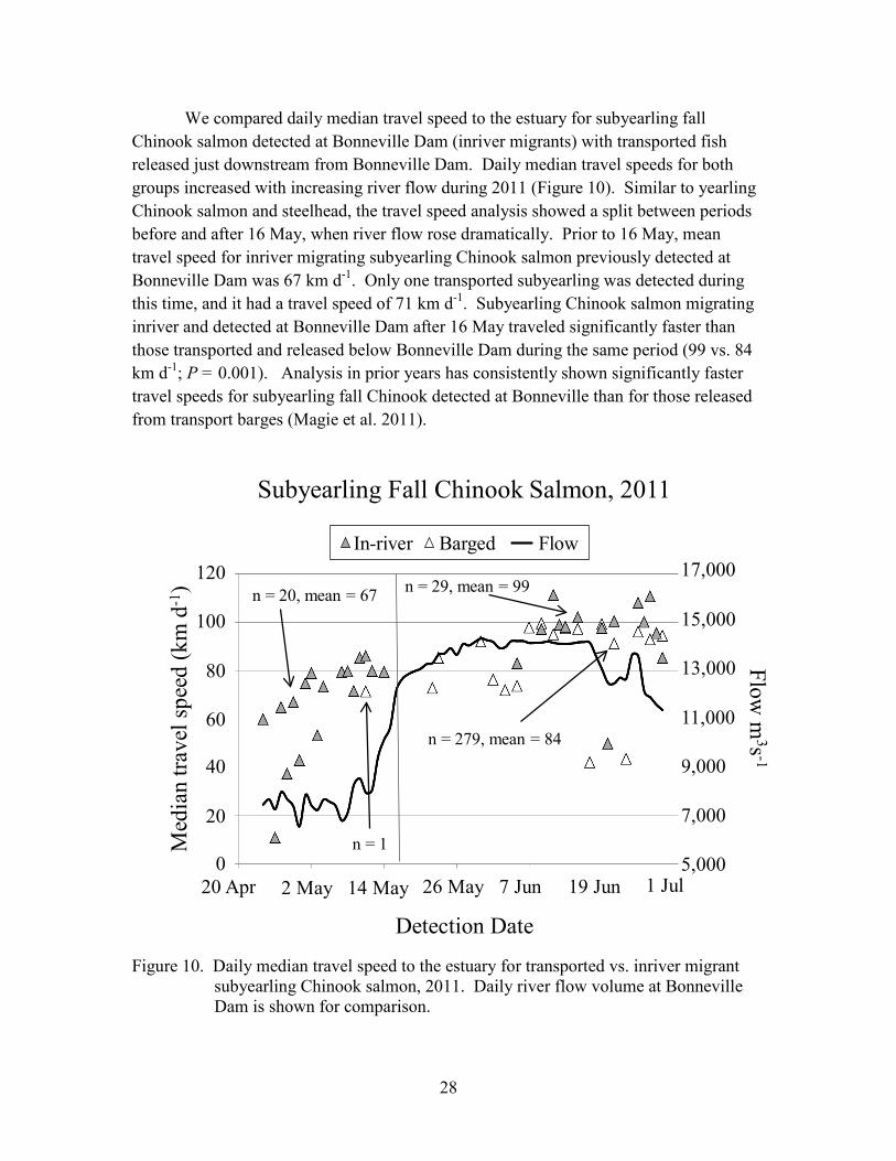
We compared daily median travel speed to the estuary for subyearling fall Chinook salmon detected at Bonneville Dam (inriver migrants) with transported fish released just downstream from Bonneville Dam. Daily median travel speeds for both groups increased with increasing river flow during 2011 (Figure 10). Similar to yearling Chinook salmon and steelhead, the travel speed analysis showed a split between periods before and after 16 May, when river flow rose dramatically. Prior to 16 May, mean travel speed for inriver migrating subyearling Chinook salmon previously detected at Bonneville Dam was 67 km d-1. Only one transported subyearling was detected during this time, and it had a travel speed of 71 km d-1. Subyearling Chinook salmon migrating inriver and detected at Bonneville Dam after 16 May traveled significantly faster than those transported and released below Bonneville Dam during the same period (99 vs. 84 km d-1; P = 0.001). Analysis in prior years has consistently shown significantly faster travel speeds for subyearling fall Chinook detected at Bonneville than for those released from transport barges (Magie et al. 2011). Figure 10. Daily median travel speed to the estuary for transported vs. inriver migrant

subyearling Chinook salmon, 2011. Daily river flow volume at Bonneville Dam is shown for comparison.

29

35

30

20

10

0

Sockeye Salmon

14 Apr 27 Apr 23 May 05 Jun 18 Jun

Detection Date

Det

ectio

ns (n

)

10 May 1 Jul

25

15

5

BargedIn-river

Sockeye Salmon—We detected 434 sockeye salmon between 15 April and 29 June (Figure 11). These fish had been released from two sites on the Snake River and five on the mainstem Columbia River. Of these 434 sockeye, 93% were hatchery origin and 1% wild, with the remaining 6% of unknown origin. The majority of these fish had migrated inriver; however, only 8 had been detected at Bonneville Dam. Of the transported sockeye, 40 were transported from Lower Granite Dam, 14 from Little Goose Dam, and 39 from Lower Monumental Dam. Sockeye released upstream from McNary Dam on the Columbia River made up 22% of our sockeye detections, while releases from the Snake River made up 78%. Less than 0.5% of these detections had been released between McNary and Bonneville Dam (Deschutes River). Mean travel speed during the intensive sample period was 105 km/d for sockeye detected at Bonneville Dam and 99 km/d for transported fish (Figure 12), but the difference was not statistically significant (P = 0.496). Figure 11. Temporal distribution for PIT-tagged sockeye salmon in the estuary, 2011.

30

In summary, travel speed from the area of Bonneville Dam to the estuary was faster for all fish groups in 2011 than in 2010, and these faster speeds can be directly attributed to the higher flow volumes. During our intensive sample period, overall flow volumes averaged 11,801 m3 s-1 in 2011 compared to 6,841 m3 s-1 in 2010 (a 72% increase). Both daily and seasonal travel speeds of fish are strongly correlated with river flow volume. Figure 12. Daily mean travel speed to the estuary for transported vs. inriver migrant

Sockeye salmon, 2011. Daily river flow volume at Bonneville Dam is shown for comparison.

Sockeye Salmon, 2011

120

100

80

60

40

20

0

15,000

13,000

11,000

9,000

7,000

5,000

Med

ian

trave

l spe

ed (k

m d

-1)

Flow m

3s -1

FlowBargedIn-river

31 Mar 15 May15 May 30 Apr 30 May 14 Jun

Detection Date

17,000n = 8, mean = 105

n = 93, mean = 99

140 19,000

31

ii10

ii10

Xday

Xday

i e1ep

βββ

βββ

++

++

+=

Detection Rates of Transported vs. Inriver Migrant Fish Methods We compared daily detection rates in the trawl between transported fish and inriver migrants previously detected at Bonneville Dam during the two-shift sample period. Detection data was evaluated to assess whether differences in detection rates were related to migration history or arrival timing in the estuary. During 2011, 159,579 yearling Chinook salmon, 571,864 subyearling Chinook salmon, and 53,680 steelhead were PIT-tagged and released for NMFS Snake River fish transportation studies. Including river-run fish diverted to barges and fish tagged and transported for other studies, a total of 78,820 yearling Chinook salmon and 49,633 steelhead were transported and released upstream from our sample site during the intensive sample period. Estuarine detection rates of PIT-tagged salmonids released from barges were compared to those of fish detected at Bonneville Dam (inriver migrants) using logistic regression (Hosmer and Lemeshow 2000; Ryan et al. 2003). Inriver migrants detected at Bonneville Dam were grouped by day of detection and paired with groups of transported fish released from a barge on the same day. Paired groups included only yearling fish released at or upstream from McNary Dam. Fish released from a barge just after midnight were grouped with fish detected the previous day at Bonneville Dam. Components of the logistic regression model were treatment as a factor and date and date-squared as covariates. The model estimated the log odds of the detection rate of the i daily cohorts (i.e., ln[pi/(1-pi)]) as a linear function of components, assuming a binomial error distribution. Daily detection rates were then estimated as: where β̂ was the coefficient of the components (i.e., 0β̂ for the intercept, 1β̂ for day i, and β̂ for the set “Xi” of day-squared and/or interaction terms). A stepwise procedure was used to determine the appropriate model. First we fit the model containing interactions between treatment and date and date-squared. We then determined the amount of overdispersion relative to that assumed from a binomial distribution (Ramsey and Schafer 1997). Overdispersion was estimated as “σ,” the square root of the model deviance statistic divided by the degrees of freedom. If σ >1.0, we adjusted the standard errors of the model coefficients by multiplying by σ (Ramsey and Schafer 1997). This inversely adjusted the z statistic used to test the significance of the coefficients, as well as appropriately inflated estimate standard errors.

32

Finally, if the interaction terms were not significant (likelihood ratio test P >0.10), these terms were removed and we fit a reduced model . The model was further reduced depending on the significance(s) between treatment and date and/or date-squared. The final model was the most reduced from this process. One constraint was that date-squared could not be in the model unless date was included as well. Various diagnostic plots were examined to assess the appropriateness of the models. Extreme or highly influential data points were identified and included or excluded on an individual basis, depending on the data situation. Fish transported early in the migration season were often released downstream from Bonneville Dam before sufficient numbers of inriver migrant fish had arrived at the dam. Recovery percentages for both inriver and transported fish groups are shown for the entire season, but were included in the analysis only when both groups were present in the daily sample. The daily barged and inriver groups had similar diel distributions in the sampling area and presumably passed the sample area at similar times. Thus, we assumed these groups were subject to the same sampling biases (sample effort). If these assumptions were correct, then differences in relative detection rates would reflect differences in survival between the two groups during passage from Bonneville Dam to the trawl. Results and Discussion Of the fish released upstream from McNary Dam and transported for NMFS transportation studies, we detected 978 yearling Chinook salmon and 1,286 steelhead in the upper estuary (Appendix Tables A5-6). We detected 281 of the 15,701 yearling Chinook salmon detected at Bonneville Dam and 263 of the 9,448 steelhead detected at Bonneville Dam (Appendix Table A7). As in previous years, a small portion of both barged and inriver migrant groups passed through the estuary either before or after the trawl-sampling period. In 2011, allowing 2 d for fish at Bonneville Dam to reach the sample area, we estimate that 73% of the barged juvenile salmonids and 65% of those detected at Bonneville Dam were at or near rkm 75 during the two-shift sample period (2 May-10 June; Table 5). These percentages were slightly lower in 2011 due to early-season index barge releases occurring when few inriver migrant fish had reached the estuary and before we instituted a second daily crew. There were also large numbers of PIT-tagged subyearling Chinook that migrated after our intensive sample period ended.

33

During the intensive sampling period, the trawl was deployed for an average of 12 h/d, and we detected 1.8% of the inriver migrant yearling Chinook and 2.8% of the inriver migrant steelhead previously detected at Bonneville Dam. By comparison, during intensive sampling in 2010, the trawl was deployed for an average of 13 h/d, and we detected 3.7% of the yearling Chinook and 4.1% of the steelhead detected at Bonneville Dam. In 2011, we also detected 1.2% of yearling Chinook salmon transported and released downstream from Bonneville Dam (vs. 3.0% in 2010), and 2.6% of steelhead transported and released downstream from Bonneville Dam (vs. 3.0% in 2010). Table 5. Trawl detection rates of PIT-tagged fish released from barges or detected

passing Bonneville Dam during the intensive sample period, 2 May-10 June 2011.

Barged fish released downstream from

Bonneville Dam Inriver fish detected at

Bonneville Dam* Released Detected % Released Detected % Chinook salmon 78,820 978 1.24 15,701 281 1.79 Steelhead 49,633 1,286 2.59 9448 263 2.78 * Selected to include only those PIT-tagged fish released at or upstream from McNary Dam, i.e., subject to

fish transportation but not transported.

Logistic regression analysis showed significant interaction between date, date-squared, or migration history (P = 0.021, 0.023, and 0.001, respectively) for yearling Chinook salmon. There were no significant interactions between date and date-squared or date-squared and migration history (P = 0.619, P = 0.990, respectively). Estimated detection rates for inriver migrants increased from around 1.1% early in the season to 2% by mid-May and then decreased to less than 0.8% by mid-June (Figure 13, top panel). Estimated detection rates for transported yearling Chinook salmon were lower early in the season (0.7%), increased to 1.4% by mid-May, and gradually decreased to 0.5% by mid-June. The adjustment for over-dispersion was 2.57. For steelhead, logistic regression analysis showed no significant interaction between migration history, date-squared, date and migration history, or date-squared and migration history (P = 0.521, 0.474, 0.151, and 0.704, respectively). There was a significant effect for date of barge release or date detected at Bonneville Dam, (P ≤ 0.001). Estimated detection rates of both barged and inriver migrant steelhead decreased steadily from early to late season (Figure 13, lower panel). Detection rates of both groups were high in early May (6.3%), declined to 2% by mid-May and 0.5% by mid-June. The adjustment for over-dispersion was 11.1.

34

For yearling Chinook salmon, the ratio of detection rates between transported fish and inriver migrants differed significantly throughout the migration season, but ranged 30-37% higher for inriver migrants than for transported fish. There were no significant differences in detection rates between migration histories for steelhead. It is possible that the lower detection rates for transported yearling Chinook salmon represent higher mortality following release from the barges than following detection at Bonneville Dam. In summary, our relative survival analysis based on estuary detection rates was confounded by low detection rates of both barged and inriver migrating fish due to the high flows in 2011. Detection rates in 2010 of fish previously detected at Bonneville Dam averaged 3.7% for yearling Chinook salmon and 4.1% for steelhead. As presented above for 2011, only early season detection rates for steelhead, obtained before the flows increased, approached the 2010 detection rates. Similarly, detection rates at Bonneville Dam were much lower in 2011 than in previous years (71% lower than in 2010). Our ability to re-sample fish known to be alive at Bonneville Dam is fundamental to estimating survival probabilities for cohorts that had remained inriver for migration.

35

01,000

3,0004,000

6,000

Tota

l Rel

ease

d (n

)

0

2

4

6

8

Det

ectio

n R

ate

(%)

Yearling Chinook Salmon, 2011n = 1,259

0

1,000

3,000

4,000

Tota

l Rel

ease

d (n

)

0

2

4

6

8

Det

ectio

n R

ate

(%)

28 Apr 8 May 18 May 28 May 07 Jun

Steelhead, 2011 n = 1,547

5,000

2,000

2,000

Barge Release In-river Release Barge %In-river % Barged Regr In-river Regr

7,0008,000

5,000

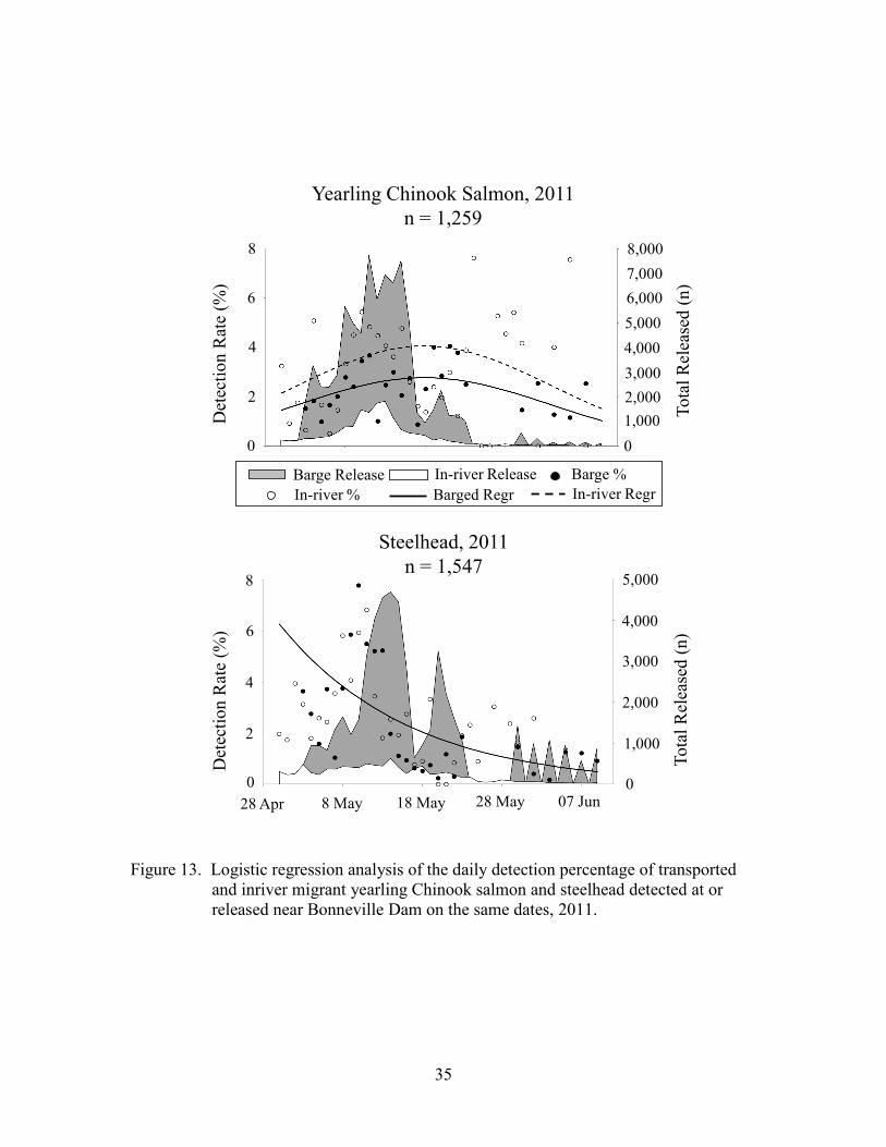
Figure 13. Logistic regression analysis of the daily detection percentage of transported

and inriver migrant yearling Chinook salmon and steelhead detected at or released near Bonneville Dam on the same dates, 2011.

36

37

DEVELOPMENT OF MOBILE SEPARATION-BY-CODE SYSTEM

Methods In 2011, we continued field testing a prototype mobile separation-by-code (MSbyC) system attached to the surface pair-trawl detection system (Magie et al. 2011). The MSbyC system was designed for use during sampling in the Columbia River estuary to detect and divert specific fish based on PIT-tag code. Diverted fish are routed to a holding tank, similar to the function of stationary SbyC systems at dams (Downing et al. 2001). These systems also allow diversion of non-tagged juvenile migrants and provide the ability to control the sample rate. Thus, this method offers a mechanism to control sample size regardless of changing fish densities, unlike traditional sampling using a beach or purse seine. A prototype MSbyC system was deployed for 10 tests in the estuary near rkm 75 during the 2010 juvenile migration season (Magie et al. 2011). During these tests, the system effectively diverted both tagged and non-tagged fish to an onboard holding tank. These deployments allowed us to assess hydraulic aspects of the system and measure delay and descaling impacts to fish. As a result of these evaluations, several modifications were suggested to improve system performance. Over the following winter, the MSbyC system underwent several modifications to improve system function and efficiency (Figure 14). A pneumatic fish-crowder was added to the fish-collection chamber (the underwater component that attaches the MSbyC equipment to the trawl). We observed the crowder area via underwater video camera, and when fish accumulated within the chamber, the crowder was operated remotely from the cabin of the vessel. This reduced fish holding and increased overall system passage. In addition, we added a water pump that was 33% larger to more effectively lift fish to the surface by increasing the area of water suction inside the fish collection chamber. The resulting increase in water volume pumped to the surface through the system required the addition of a water control device (drier) on deck. The drier enabled the removal of over half of the water volume. These improvements were intended to entrain more fish in the system and reduce turbulence downstream of the drier. We also incorporated the use of air bubblers positioned at the bottom of the collection tube to further influence fish to enter the area of flow entrainment. The primary goal of MSbyC deployments in 2011 was to test these modifications in an active sampling environment.

38

Figure 14. Diagram of the mobile system designed to divert fish by PIT-tag code after

passing through the trawl, including modifications made during the winter of 2010-2011.

Deployments of the MSbyC system were originally planned to begin in early spring, when few fish would be present. Once safe operational procedures and full functionality were established, we planned weekly deployments to continue through the juvenile salmon migration season. Our goals were to collect samples of fish with known migration histories and to monitor the species composition of non-tagged fish passing through the system. However, delays in fabrication and engineering issues precluded conclusive testing of impacts to fish and until after the majority of yearling fish had migrated through the estuary. We were able to conduct a single deployment of the MSbyC in late June, when subyearling Chinook salmon were the predominant species.

39

During the single deployment, we first established system function (flow settings) and switch-gate timing by incrementally introducing wooden dowels implanted with PIT tags (stick fish) in front of the two in-series detection coils. We also monitored fish activity and mechanical function of the fish crowder in the underwater collection chamber with underwater cameras. Two cameras faced towards the rear of the chamber and one faced forward into the trawl. Operators observed fish movement into the chamber and through the pump intake. When debris accumulated or adult fish were present, an operator would open the 0.9-m-diameter pneumatic screen at the rear of the chamber to allow all debris or adult fish to clear the system. The underwater video cameras also allowed operators to direct fish toward the pump intake and encourage passage through the system by manually activating the crowder, which was mounted on the ceiling, and the air bubblers, which were mounted on the bottom of the collection chamber. We diverted all PIT-tagged fish, and during two short timed periods based on fish densities observed in the fish chamber, we diverted all fish to the sample tank. Non-tagged fish were used to determine species composition and health of all fish passing through the trawl at that time. Collected fish were anesthetized, identified to species, and measured for fork length, clips, descaling, predatory marks, and injuries.

Results and Discussion On 24 June 2011 the prototype MSbyC system was deployed for 2.3 h and a total of four PIT-tagged fish were detected in the system and successfully diverted into the sample tank. Few non-tagged fish were diverted during this period. We recorded data for all four PIT-tagged fish with known migration histories (Table 6). All four of these fish were subyearling Chinook salmon that had originated in the Snake River or a tributary of the Snake River. Based upon fork-lengths at recapture, growth rates since tagging ranged from 0.24 to 0.43 mm d-1 with a mean rate of 0.33 mm d-1. This small dataset is representative of the several potential biological samples possible from fish migrating through the estuary using an MSbyC system. We also locked the diversion gate in the "sample" position (to divert all passing fish) for two short periods, again based on numbers of fish observed accumulating in the fish collection chamber. These sample periods totaled 2.5 minutes, and we diverted 92 non-tagged subyearling Chinook salmon and two steelhead (Table 7). Of the 96 total yearling Chinook salmon sampled with the MSbyC, including tagged and non-tagged fish, median fork length was 86 mm (n = 45) for hatchery fish (as determined by adipose fin clip), and 84 mm for fish with an intact adipose fin (n = 51).

40

Table 6. Growth rates of PIT-tagged fish from release (PTAGIS designation) to recovery in the Columbia River estuary using the MSbyC system, 2011.

PIT-tagged salmon sampled using MSbyC

Species Rear type Migration Release site Release date Length at MSbyC

Length at tagging

Growth rate (mm/day)

Chinook Hatchery Barged SNAKE3 6/03/2011 6:00 PM 90 85 0.24 Chinook Hatchery Barged SNAKE3 6/02/2011 12:00 PM 105 76 0.43 Chinook Hatchery Barged SNAKE3 6/06/2011 7:20 PM 85 78 0.39 Chinook Hatchery River Run GRAND1 5/24/2011 12:00 PM 98 82 0.25

We also measured length for the two steelhead collected using the MSbyC system; one of these fish was adipose-fin clipped (240 mm) and the other was not (200 mm). These samples are representative of data obtainable using a fish-density independent strategy to sample ESA listed populations in the estuary. The relatively short duration of the sample was made possible by concentrating river-run fish to a collection point using a large surface pair-trawl. We believe a biweekly sample of 300 fish would provide a known context of overall species composition in the estuary on the dates when PIT-tagged fish are subsampled from the total collection in the trawl. Table 7. Median fork length of fish collected during the 2.5 minute full diversion sample.

Adipose clipped Adipose intact

n Median length (mm) n Median length (mm) Chinook 45 86 51 84 Steelhead 1 240 1 200 During initial deployment of the MSbyC in 2010, the rate of significant descaling and injury was 9% early in the season. We made corrective modifications in the field which included adding baffling in the sample tank and increasing the discharge capacity of the water drier in front of the sample tank. These changes reduced flow and turbulence in the tank and lowered the descaling and injury rate to 2% during subsequent deployments. Additional modification were suggested and implemented as described above over the winter at our Pasco, WA shop facility in 2010-2011. Unfortunately, these modifications increased the weight of the craft and challenged its structural integrity.

41

A single deployment was allowed by the NOAA small boat program after removal of about 500 pounds from the vessel (outboard motor). This deployment confirmed that the modifications improved the MSbyC system but was not sufficient to fully assess impacts to fish health or operational efficiencies. While there remains a need for further testing, this system offers a low impact, fish density independent method to sample actively migrating juvenile salmonids of known migration history (inriver or transported) after they co-mingle in the estuary.

42

43

REFERENCES Axel, A. A., E. E. Hockersmith, B. J. Burke, K. Frick, B. P. Sandford, W. D. Muir, R. F.

Absolon, N. Dumdei, J. J. Lamb, and M. G. Nesbit. 2010. Passage behavior and survival of radio-tagged yearling and subyearling Chinook salmon and juvenile steelhead at Ice Harbor Dam, 2009. Report to the Army Corps of Engineers, Walla Walla, Washington.

Connor, W. P., J. G. Sneva, K. F. Tiffan, R. K. Steinhorst, and D. Ross. 2005. Two

alternative juvenile life history types for fall Chinook salmon in the Snake River Basin. Transactions of the American Fisheries Society 134: 291-304.

Cormack, R. M. 1964. Estimates of survival from the sightings of marked animals.

Biometrika 51:429-483. Downing, S. L., E. F. Prentice, B. W. Peterson, E. P. Nunnallee, and B. F. Jonasson.

2001. Development and evaluation of passive integrated transponder tag technology. Report of the National Marine Fisheries Service to the Bonneville Power Administration, Portland, Oregon.

Faulkner, J. R., S. G. Smith, W. D. Muir, D. M. Marsh, and R. W. Zabel. 2012.

Survival estimates for the passage of spring-migrating juvenile salmonids through Snake and Columbia River dams and reservoirs, 2011. Report of the National Marine Fisheries Service to the Bonneville Power Administration, Portland, Oregon.

Hockersmith, E. E., G. A. Axel, R. F. Absolon, B. J. Burke, K. E. Frick, J. J. Lamb, M.

G. Nesbit, N. D. Dumbdei, and B. P. Sandford. 2010. Passage behavior and survival for radio-tagged yearling Chinook salmon and juvenile steelhead at Lower Monumental Dam, 2009. Report to the Army Corps of Engineers, Walla Walla, Washington.

Hosmer, D. W., and S. Lemeshow. 2000. Applied Logistic Regression, 2nd ed. John

Wiley & Sons, Inc., 375 pp. Jolly, G. M. 1965. Explicit estimates from capture-recapture data with both death and

immigration—stochastic model. Biometrika 52:225-247. Ledgerwood, R. D., F. P. Thrower, and E. M. Dawley. 1991. Diel sampling of migratory

juvenile salmonids in the Columbia River Estuary. U.S. Fishery Bulletin 68:203-217.

44

Ledgerwood, R. D. J. W. Ferguson, B. A. Ryan, E. M. Dawley, and E. P. Nunnallee. 2004. A surface trawl to detect migrating juvenile salmonids tagged with passive integrated transponder tags. North American Journal of Fisheries Management 24:440-451.

Ledgerwood, R. D., A. S. Cameron, B. P. Sandford, L. B. Way, and G. M. Matthews.

2005. Detection of PIT-tagged juvenile salmonids in the Columbia River estuary using a pair-trawl, 2002. Report of the National Marine Fisheries Service to the U.S. Army Corps of Engineers, Walla Walla, Washington.

Magie, R. J., M. S. Morris, R. D. Ledgerwood, A. L. Cook, B. P. Sandford, and G. M.

Matthews. 2010. Detection of PIT-tagged juvenile salmonids in the Columbia River estuary using pair-trawls, 2008. Report of the National Marine Fisheries Service to the U.S. Army Corps of Engineers, Walla Walla, Washington.

Magie, R. J., M. S. Morris, R. D. Ledgerwood, A. L. Cook, and B. P. Sandford. 2011.

Detection of PIT-tagged juvenile salmonids in the Columbia River estuary using pair-trawls, 2010. Report of the National Marine Fisheries Service to the U.S. Army Corps of Engineers, Walla Walla, Washington.

Marsh, D. M., J. R. Harmon, N. N. Paasch, K. L. Thomas, K. W. McIntyre, B. P.

Sandford, G. M. Matthews. 2005. Research related to transportation of juvenile salmonids on the Columbia and Snake Rivers, 2004: final report for the 2001 spring/summer Chinook salmon juvenile migration. Report of the National Marine Fisheries Service to the U.S. Army Corps of Engineers Walla Walla, Washington.

Marsh, D. M. J. R. Harmon, N. N. Paasch, K. L. Thomas, K. W. McIntyre, B. P.

Sandford, and G. M. Matthews. 2010. Transport of juvenile salmonids on the Snake River, 2007: final report for the 2004 wild spring/summer Chinook salmon juvenile migration. Draft report of the National Marine Fisheries Service to the U.S. Army Corps of Engineers, Walla Walla, Washington.

Marsh, D. M., J. R. Harmon, N. N. Paasch, K. L. Thomas, K. W. McIntyre, B. P.

Sandford, G. M. Matthews, and W. D. Muir. 2008. Transportation of juvenile salmonids on the Snake River, 2005: Final report for 2003 steelhead juveniles with updates on other transport studies. Report of the National Marine Fisheries Service to the U.S. Army Corps of Engineers Walla Walla, Washington.

Marsh, D. M., W. D. Muir, B. P. Sandford, S. G. Smith, and Diane Elliott. 2012.

Alternative barging strategies to improve survival of salmonids transported from Lower Granite Dam: final report from the 2006-2008 spring/summer Chinook salmon and steelhead juvenile migration. Report of the National Marine Fisheries Service to the U.S. Army Corps of Engineers Walla Walla, Washington.

45

Muir, W. D., S. G. Smith, J. G. Williams, E. E. Hockersmith, and J. R. Skalski. 2001. Survival estimates for migrant yearling chinook salmon and steelhead tagged with passive integrated transponders in the lower Snake and lower Columbia Rivers, 1993-1998. North American Journal of Fisheries Management 21:269-282.

Prentice, E. F., T. A. Flagg, and C. S. McCutcheon. 1990a. Electronic tags. American

Fisheries Society Symposium 7:317-322. Prentice, E. F., T. A. Flagg, C. S. McCutcheon, and D. F. Brastow. 1990b. PIT-tag

monitoring systems for hydroelectric dams and fish hatcheries. American Fisheries Society Symposium 7:323-334.

Prentice, E. F., T. A. Flagg, C. S. McCutcheon, D. F. Brastow, and D. C. Cross. 1990c.

Equipment, methods, and an automated data-entry station for PIT tagging. American Fisheries Society Symposium 7:335-340.

PSMFC (Pacific States Marine Fisheries Commission). 2010. The Columbia Basin

PIT-Tag-Information System (PTAGIS). Online interactive database, Pacific States Marine Fisheries Commission, Gladstone, Oregon (available via the internet at www.psmfc.org/pittag).

Ramsey, F., and Schafer, D. 1997. The Statistical Sleuth. Duxbury Press. Ryan, B. A., S. G. Smith, J. M. Butzerin, and J. W. Ferguson. 2003. Relative

vulnerability to avian predation of PIT-tagged juvenile salmonids in the Columbia River estuary, 1998-2000. Transactions of the American Fisheries Society. 132:275-288.

Seber, G. A. F. 1965. A note on the multiple recapture census. Biometrika 52:249-259. Skalski, J. R., S. G. Smith, R. N. Iwamoto, J. G. Williams, and A. Hoffmann. 1998. Use

of passive integrated transponder tags to estimate survival of migrant juvenile salmonids in the Snake and Columbia Rivers. Canadian Journal of Fisheries and Aquatic Sciences 55:1484-1493.

Stein, C., D. Marvin, J. Tenney, and N. Gruman, editors. 2004. 2004 PIT tag

specification document. Report of the Pacific States Marine Fisheries Commission to the PIT tag Technical Steering Committee. Gladstone, Oregon (available via the internet at www.psmfc.org/pittag).

Williams, J. G., S. G. Smith, and W. D. Muir. 2001. Survival estimates for downstream

migrant-yearling juvenile salmonids through the Snake and Columbia River hydropower system, 1966 to 1980 and 1993 to 1999. North American Journal of Fisheries Management 21:310-317.

46

Zabel, R. W. and J. G. Williams. 2002. Selective mortality for fish length and migrational timing in chinook salmon: what is the role of human disturbance? Ecological Applications 12:173-183.

Zar, J. H. 1999. Biostatistical analysis, 4th edition. Prentice Hall, Upper Saddle River,

New Jersey.

47

APPENDIX A

Data Tables Appendix Table A1. Daily total sample time and detections for each salmonid species

using the matrix pair trawl antenna system at Jones Beach, 2011.

Date Sample

Time (h)

PIT-tag detections (N)

Unknown Chinook Salmon

Coho Salmon Steelhead

Sockeye Salmon Cutthroat Total

22 Mar 2.27 0 0 0 0 0 0 0 23 Mar 5.20 0 0 0 0 0 0 0 24 Mar 0.00 -- -- -- -- -- -- -- 25 Mar 5.65 0 0 0 0 0 0 0 26 Mar 0.00 -- -- -- -- -- -- -- 27 Mar 0.00 -- -- -- -- -- -- -- 28 Mar 2.38 0 1 0 0 0 0 1 29 Mar 0.00 -- -- -- -- -- -- -- 30 Mar 0.00 -- -- -- -- -- -- -- 31 Mar 0.00 -- -- -- -- -- -- -- 1 Apr 4.83 0 2 0 0 0 0 2 2 Apr 0.00 -- -- -- -- -- -- -- 3 Apr 0.00 -- -- -- -- -- -- -- 4 Apr 4.28 0 1 0 0 0 0 1 5 Apr 0.00 -- -- -- -- -- -- -- 6 Apr 2.93 0 0 0 0 0 0 0 7 Apr 0.00 -- -- -- -- -- -- -- 8 Apr 0.00 -- -- -- -- -- -- -- 9 Apr 0.00 -- -- -- -- -- -- -- 10 Apr 0.00 -- -- -- -- -- -- -- 11 Apr 0.00 -- -- -- -- -- -- -- 12 Apr 0.00 -- -- -- -- -- -- -- 13 Apr 5.57 0 1 0 4 0 0 5 14 Apr 6.15 0 2 0 4 0 0 6 15 Apr 6.18 0 5 0 11 1 0 17 16 Apr 5.75 0 4 0 6 0 0 10 17 Apr 0.00 -- -- -- -- -- -- -- 18 Apr 5.35 0 1 0 7 0 0 8 19 Apr 0.00 -- -- -- -- -- -- -- 20 Apr 6.25 1 2 0 7 0 0 10 21 Apr 5.70 1 1 0 9 0 0 11 22 Apr 4.08 1 2 0 1 0 0 4 23 Apr 0.00 -- -- -- -- -- -- -- 24 Apr 0.00 -- -- -- -- -- -- -- 25 Apr 6.28 2 7 0 22 0 0 31 26 Apr 7.15 0 10 0 17 0 0 27 27 Apr 6.25 0 11 0 23 0 0 34 28 Apr 6.87 1 9 0 21 0 0 31 29 Apr 5.93 0 5 1 10 0 0 16 30 Apr 6.62 1 12 0 32 0 0 45 1 May 4.92 1 18 0 38 0 0 57

48

Appendix Table A1. Continued.

Date Sample

Time (h)

PIT-tag detections (N)

Unknown Chinook Salmon

Coho Salmon Steelhead

Sockeye Salmon Cutthroat Total

2 May 11.53 1 49 1 50 0 0 101 3 May 9.87 1 56 0 30 0 0 87 4 May 13.92 2 35 1 113 0 0 151 5 May 11.77 1 42 1 106 0 0 150 6 May 13.30 5 132 0 95 0 0 232 7 May 7.63 2 55 0 48 0 0 105 8 May 11.18 3 97 0 106 1 0 207 9 May 11.65 5 111 0 65 0 0 181 10 May 15.13 19 264 0 222 1 0 506 11 May 16.28 19 302 1 225 1 0 548 12 May 17.53 29 475 0 391 2 0 897 13 May 16.68 24 478 2 329 4 0 837 14 May 12.35 26 265 1 409 4 0 705 15 May 13.55 46 371 4 469 7 0 897 16 May 16.83 54 433 7 301 11 0 806 17 May 13.77 63 408 7 215 1 1 695 18 May 11.17 42 334 7 143 5 0 531 19 May 9.38 40 283 8 180 11 0 522 20 May 12.98 30 310 6 125 4 0 475 21 May 7.95 23 182 5 136 7 0 353 22 May 10.35 17 192 5 105 5 0 324 23 May 13.73 29 265 10 160 13 0 477 24 May 13.28 17 237 15 124 22 0 415 25 May 13.37 17 222 23 157 37 0 456 26 May 11.10 10 93 10 72 1 0 186 27 May 10.97 12 62 10 53 3 0 140 28 May 7.02 6 33 6 60 3 0 108 29 May 9.67 7 63 8 71 17 0 166 30 May 8.82 8 70 12 66 16 0 172 31 May 9.80 3 45 9 70 22 0 149 1 Jun 11.62 5 55 18 75 40 0 193 2 Jun 10.82 8 57 13 80 27 0 185 3 Jun 10.60 4 54 14 54 40 0 166 4 Jun 7.02 1 17 6 23 13 0 60 5 Jun 10.48 2 62 13 37 33 0 147 6 Jun 11.53 4 66 21 33 19 0 143 7 Jun 11.13 2 68 12 31 17 0 130 8 Jun 11.00 2 49 13 27 8 0 99 9 Jun 11.10 4 60 10 18 13 0 105 10 Jun 11.55 1 60 15 32 11 0 119 11 Jun 7.00 1 57 6 12 3 0 79 12 Jun 0.00 -- -- -- -- -- -- -- 13 Jun 3.68 1 64 3 11 1 0 80 14 Jun 5.28 1 47 4 26 1 0 79 15 Jun 4.92 2 48 2 11 3 0 66 16 Jun 5.40 0 63 6 5 1 0 75 17 Jun 5.12 0 75 2 11 4 0 92 18 Jun 0.00 -- -- -- -- -- -- -- 19 Jun 0.00 -- -- -- -- -- -- -- 20 Jun 6.20 1 40 1 5 0 0 47

49

Appendix Table A1. Continued.

Date Sample

Time (h)

PIT-tag Detections (N)

Unknown Chinook Salmon

Coho Salmon Steelhead

Sockeye Salmon Total

21 Jun 5.77 0 44 1 7 0 0 52 22 Jun 5.82 0 24 0 1 0 0 25 23 Jun 5.67 0 44 0 5 0 0 49 24 Jun 2.30 0 4 0 0 0 0 4 25 Jun 0.00 -- -- -- -- -- -- -- 26 Jun 0.00 -- -- -- -- -- -- -- 27 Jun 5.62 0 55 0 5 0 0 60 28 Jun 5.72 0 36 2 2 0 0 40 29 Jun 5.23 0 69 1 1 1 0 72 30 Jun 5.97 0 17 1 2 0 0 20 1 Jul 5.68 0 37 1 3 0 0 41 Total 671.38 608 7,330 325 5,425 434 1 14,123

50

Appendix Table A2. Release and consecutive observation sites and dates for the 18 subyearling Chinook salmon that were released in 2010 and detected in 2011. Overwintering location is between the last detection site in 2010 and the first detection site in 2011.

Tag ID Release/Observation site Release/Observation date 3D9.1C2D22F58A CJRAP 4/5/2010 15:00 3D9.1C2D22F58A TWX 5/10/2011 5:30

3D9.1C2D31E26F SNAKE3 5/20/2010 23:40 3D9.1C2D31E26F GOJ 4/2/2011 2:13 3D9.1C2D31E26F TWX 5/10/2011 0:44

3D9.1C2D4AA1E0 BCCAP 7/7/2010 18:40 3D9.1C2D4AA1E0 GRJ 10/27/2010 19:38 3D9.1C2D4AA1E0 TWX 5/1/2011 19:33

3D9.1C2D4B95E5 BCCAP 7/7/2010 18:40 3D9.1C2D4B95E5 GOJ 4/19/2011 13:52 3D9.1C2D4B95E5 ICH 5/1/2011 11:42 3D9.1C2D4B95E5 MCJ 5/9/2011 12:58 3D9.1C2D4B95E5 JDJ 5/12/2011 21:20 3D9.1C2D4B95E5 TWX 5/15/2011 21:45

3D9.1C2D4BAD58 BCCAP 6/30/2010 20:00 3D9.1C2D4BAD58 JDJ 4/10/2011 20:16 3D9.1C2D4BAD58 TWX 4/14/2011 8:36

3D9.1C2D4BBFF4 BCCAP 7/9/2010 18:30 3D9.1C2D4BBFF4 GOJ 3/22/2011 15:53 3D9.1C2D4BBFF4 TWX 5/1/2011 20:22

3D9.1C2D4E87F7 BCCAP 6/23/2010 16:50 3D9.1C2D4E87F7 GRJ 3/25/2011 22:39 3D9.1C2D4E87F7 GOJ 4/8/2011 15:12 3D9.1C2D4E87F7 LMJ 4/11/2011 19:26 3D9.1C2D4E87F7 MCJ 5/2/2011 8:07 3D9.1C2D4E87F7 TWX 5/10/2011 22:27

3D9.1C2D52E85D BCCAP 5/25/2010 8:00 3D9.1C2D52E85D TWX 5/21/2011 10:38

3D9.1C2D58E254 BCCAP 6/25/2010 15:00 3D9.1C2D58E254 GRJ 12/12/2010 8:37 3D9.1C2D58E254 LMJ 4/7/2011 15:25 3D9.1C2D58E254 MCJ 5/2/2011 19:30 3D9.1C2D58E254 TWX 5/14/2011 10:58

3D9.1C2D5A1BB3 SNAKE3 5/31/2010 20:00 3D9.1C2D5A1BB3 MCJ 10/7/2010 14:42 3D9.1C2D5A1BB3 TWX 4/28/2011 7:52

3D9.1C2D5BD691 SNAKE3 6/2/2010 17:30 3D9.1C2D5BD691 TWX 4/14/2011 12:26

51

Appendix Table A2. Continued. Tag ID Release/Observation site Release/Observation date 3D9.1C2D5F2135 BCCAP 6/25/2010 15:00 3D9.1C2D5F2135 GRJ 5/10/2011 5:11 3D9.1C2D5F2135 LMJ 5/14/2011 16:41 3D9.1C2D5F2135 JDJ 5/21/2011 0:09 3D9.1C2D5F2135 TWX 5/24/2011 0:17

3D9.1C2D5F2D33 BCCAP 6/24/2010 18:40 3D9.1C2D5F2D33 GRJ 10/8/2010 7:26 3D9.1C2D5F2D33 JDJ 4/28/2011 15:05 3D9.1C2D5F2D33 TWX 5/2/2011 21:41

3D9.1C2D5F30A4 BCCAP 7/1/2010 18:25 3D9.1C2D5F30A4 GOJ 4/4/2011 16:18 3D9.1C2D5F30A4 BCC 4/14/2011 8:06 3D9.1C2D5F30A4 TWX 4/16/2011 10:34

3D9.1C2D5F5124 BCCAP 7/1/2010 18:25 3D9.1C2D5F5124 GRJ 10/7/2010 17:29 3D9.1C2D5F5124 GOJ 11/30/2010 2:56 3D9.1C2D5F5124 MCJ 4/29/2011 17:37 3D9.1C2D5F5124 TWX 5/6/2011 7:58

3D9.1C2D5F6CEE BCCAP 7/1/2010 18:25 3D9.1C2D5F6CEE TWX 5/15/2011 21:11

3D9.1C2D5FA722 BCCAP 7/1/2010 18:25 3D9.1C2D5FA722 GOJ 12/7/2010 20:37 3D9.1C2D5FA722 LMJ 12/16/2010 21:25 3D9.1C2D5FA722 TWX 4/18/2011 11:09

3D9.1C2D631CE1 BCCAP 7/1/2010 18:25 3D9.1C2D631CE1 TWX 4/4/2011 10:59

52

Appendix Table A3. Combined daily total of impinged or injured fish on the matrix antenna system used in the upper Columbia River estuary, 2011.

Chinook Salmon

Date Yearling Subyearling Coho Steelhead Sockeye 22 Mar 0 0 0 0 0 23 Mar 0 0 0 0 0 24 Mar -- -- -- -- -- 25 Mar 0 0 0 0 0 26 Mar -- -- -- -- -- 27 Mar -- -- -- -- -- 28 Mar 0 0 0 0 0 29 Mar -- -- -- -- -- 30 Mar 0 0 0 0 0 31 Mar -- -- -- -- -- 1 Apr 0 0 0 0 0 2 Apr -- -- -- -- -- 3 Apr -- -- -- -- -- 4 Apr 0 0 0 0 0 5 Apr -- -- -- -- -- 6 Apr 0 0 0 0 0 7 Apr -- -- -- -- -- 8 Apr -- -- -- -- -- 9 Apr -- -- -- -- -- 10 Apr -- -- -- -- -- 11 Apr -- -- -- -- -- 12 Apr -- -- -- -- -- 13 Apr 0 0 0 0 0 14 Apr 0 0 0 0 0 15 Apr 5 0 0 2 0 16 Apr 0 0 0 0 0 17 Apr -- -- -- -- -- 18 Apr 1 0 0 0 0 19 Apr -- -- -- -- -- 20 Apr 0 0 0 0 0 21 Apr 1 0 0 0 0 22 Apr 0 0 0 0 0 23 Apr -- -- -- -- -- 24 Apr -- -- -- -- -- 25 Apr 0 0 0 0 0 26 Apr 2 0 0 0 0 27 Apr 0 0 0 0 0 28 Apr 2 0 0 0 0 29 Apr 1 0 0 0 0 30 Apr 0 0 0 0 0 1 May 3 0 0 0 0 2 May 0 0 0 0 0 3 May 0 0 0 0 0 4 May 0 0 0 0 0 5 May 0 0 0 0 0 6 May 2 0 0 1 0 7 May 1 0 0 2 0 8 May 2 0 1 2 0 9 May 1 0 0 0 0 10 May 0 0 0 0 0 11 May 0 0 0 0 0 12 May 2 0 0 0 0

53

Appendix Table A3. Continued.

Chinook Salmon

Date Yearling Subyearling Coho Steelhead Sockeye 13 May 2 0 0 0 0 14 May 0 0 0 0 0 15 May 0 0 0 0 0 16 May 2 0 1 1 0 17 May 2 0 0 0 0 18 May 4 0 3 2 1 19 May 1 0 0 0 0 20 May 2 0 1 1 0 21 May 2 0 0 1 0 22 May 1 0 0 1 0 23 May 1 0 0 2 0 24 May 1 0 1 0 1 25 May 1 0 1 2 4 26 May 2 0 0 0 1 27 May 0 0 0 0 0 28 May 0 0 0 0 0 29 May 0 0 0 0 1 30 May 0 0 0 0 0 31 May 0 0 0 0 0 1 Jun 1 0 0 0 1 2 Jun 0 0 0 0 0 3 Jun 0 0 0 0 0 4 Jun 0 0 0 0 1 5 Jun 0 0 0 0 1 6 Jun 1 0 0 0 0 7 Jun 0 0 0 0 1 8 Jun 0 0 0 0 0 9 Jun 0 0 0 0 0 10 Jun 1 0 0 0 0 11 Jun 0 0 0 0 0 12 Jun -- -- -- -- -- 13 Jun 0 0 0 0 0 14 Jun 0 0 0 0 0 15 Jun 0 0 0 0 0 16 Jun 0 0 0 0 0 17 Jun 1 0 0 0 1 18 Jun -- -- -- -- -- 19 Jun -- -- -- -- -- 20 Jun 1 0 0 1 0 21 Jun 2 0 0 0 0 22 Jun 1 0 0 0 0 23 Jun 0 0 0 0 0 24 Jun -- -- -- -- -- 25 Jun -- -- -- -- -- 26 Jun -- -- -- -- -- 27 Jun 1 0 0 1 0 28 Jun 0 0 0 0 0 29 Jun 2 0 0 0 0 30 Jun 1 0 0 1 0 1 Jul 0 0 0 0 0 Total 56 0 8 20 13

54

Appendix Table A4. Diel sampling of yearling Chinook salmon and steelhead using a PIT-tag detector surface pair-trawl at Jones Beach (rkm 75), 2011. Two-crew effort (2 May-10 June) was rounded to the nearest tenth and presented as a decimal hour.

Diel hour Effort (h)

Yearling Chinook salmon Steelhead n n/h n n/h

Hatchery Wild Hatchery Wild Hatchery Wild Hatchery Wild 0 33.5 315 47 9.4 1.4 93 40 2.8 1.2 1 32.9 335 52 10.2 1.6 118 33 3.6 1.0 2 15.3 218 22 14.3 1.4 36 6 2.4 0.4 3 5.7 103 13 18.0 2.3 14 4 2.4 0.7 4 1.5 0 0 0.0 0.0 1 0 0.7 0.0 5 0.1 1 0 10.0 0.0 0 0 0.0 0.0 6 20.4 118 27 5.8 1.3 90 26 4.4 1.3 7 39.3 369 84 9.4 2.1 332 88 8.5 2.2 8 40.0 505 112 12.6 2.8 521 122 13.0 3.1 9 40.0 374 66 9.4 1.7 425 129 10.6 3.2 10 39.2 384 70 9.8 1.8 506 119 12.9 3.0 11 36.6 288 53 7.9 1.4 526 112 14.4 3.1 12 17.6 181 45 10.3 2.6 341 81 19.4 4.6 13 11.2 165 25 14.7 2.2 241 66 21.5 5.9 14 8.3 95 18 11.5 2.2 153 41 18.5 5.0 15 1.3 0 1 0.0 0.8 1 0 0.8 0.0 16 0.0 -- -- -- -- -- -- -- -- 17 0.0 -- -- -- -- -- -- -- -- 18 0.0 -- -- -- -- -- -- -- -- 19 4.1 15 7 3.7 1.7 23 10 5.6 2.4 20 22.4 203 51 9.1 2.3 65 35 2.9 1.6 21 33.5 594 120 17.7 3.6 138 49 4.1 1.5 22 33.1 418 55 12.6 1.7 110 48 3.3 1.5 23 33.9 314 51 9.3 1.5 72 33 2.1 1.0 Total 470 4,995 919 3,806 1,042

55

Appendix Table A5. Number of PIT-tagged yearling Chinook salmon loaded for transport at dams and numbers detected in the estuary. LGR, Lower Granite; LGO, Little Goose; LMN, Lower Monumental. Transport dates 8 Apr - 1 Jul; trawl operation 22 Mar - 1 Jul, with intensive sampling 2 May - 10 Jun 2011. Season totals are shown.

Release date and time

Numbers loaded at each dam and total fish loaded (n) Percent detected from each dam and total numbers detected (n) LGR LGO LMN N LGR LGO LMN n (%)

4/8/11 7:45 PM 876 0 0 876 0.46 -- -- 4 0.46 4/15/11 8:15 PM 1,562 0 0 1,562 0.38 -- -- 6 0.38 4/22/11 8:00 PM 1,309 0 0 1,309 0.38 -- -- 5 0.38 4/29/11 9:10 PM 1,391 0 0 1,391 0.86 -- -- 12 0.86 5/3/11 8:25 PM 1,704 0 0 1,704 0.76 -- -- 13 0.76 5/4/11 8:30 PM 3,273 0 0 3,273 0.92 -- -- 30 0.92 5/5/11 8:25 PM 2,415 0 0 2,415 0.50 -- -- 12 0.50 5/6/11 7:35 PM 2,393 0 0 2,393 0.84 -- -- 20 0.84 5/7/11 8:40 PM 2,632 251 0 2,883 0.99 1.20 -- 29 1.01 5/8/11 8:30 PM 3,238 2,430 0 5,668 1.36 1.44 -- 79 1.39 5/9/11 9:00 PM 2,881 2,116 1 4,998 1.08 1.37 0 60 1.20 5/10/11 9:00 PM 2,257 2,118 202 4,577 1.51 1.79 3.47 79 1.73 5/11/11 10:50 PM 4,332 2,035 1,378 7,745 1.52 2.16 2.32 142 1.83 5/12/11 8:30 PM 3,585 1,587 780 5,952 0.50 0.32 0.90 30 0.50 5/13/11 9:20 PM 3,805 2,071 1,082 6,958 1.02 1.30 1.85 86 1.24 5/14/11 8:00 PM 2,610 2,748 1,262 6,620 1.03 1.82 1.74 99 1.50 5/15/11 8:25 PM 2,770 2,021 2,727 7,518 0.65 0.94 1.47 77 1.02 5/16/11 8:30 PM 1,600 1,269 2,218 5,087 0.75 1.50 1.76 70 1.38 5/17/11 1:45 PM 0 1,355 7 1,362 -- 0.44 0 6 0.44 5/18/11 8:30 PM 0 953 0 953 -- 1.15 -- 11 1.15 5/19/11 11:25 PM 0 1,449 0 1,449 -- 2.00 -- 29 2.00 5/20/11 9:00 PM 479 952 826 2,257 2.09 1.16 1.33 32 1.42 5/21/11 8:55 PM 300 435 500 1,235 1.00 1.38 3.20 25 2.02 5/22/11 8:50 PM 552 265 453 1,270 2.36 1.89 1.32 24 1.89 5/23/11 7:05 PM 228 328 483 1,039 1.75 1.83 0.62 13 1.25

56

Appendix Table A5. Continued.

Release date and time

Numbers loaded at each dam and total fish loaded (n) Percent detected from each dam and total numbers detected (n) LGR LGO LMN N LGR LGO LMN n (%)

5/30/11 7:55 PM 212 0 332 544 0.94 -- 0.60 4 0.74 6/1/11 9:05 PM 98 0 217 315 3.06 -- 0.46 4 1.27 6/3/11 7:50 PM 103 13 41 157 0.97 0 0 1 0.64 6/5/11 8:50 PM 89 71 13 173 1.12 0 0 1 0.58 6/7/11 8:45 PM 87 47 24 158 1.15 2.13 0 2 1.27 6/9/11 8:30 PM 79 31 7 117 0 0 0 0 0 6/11/11 6:20 PM 100 42 0 142 2.00 2.38 -- 3 2.11 6/13/11 9:00 PM 53 57 25 135 1.89 3.51 0 3 2.22 6/15/11 8:20 PM 30 36 15 81 6.67 2.78 0 3 3.70 6/17/11 8:00 PM 28 24 12 64 0 0 0 0 0 6/19/11 8:30 PM 32 11 6 49 0 0 0 0 0 6/21/11 6:00 PM 17 20 10 47 0 0 0 0 0 6/23/11 8:45 PM 16 9 13 38 0 0 0 0 0 6/25/11 7:30 PM 11 13 2 26 0 0 0 0 0 6/27/11 6:00 PM 37 16 7 60 2.70 0 14.29 2 3.33 6/29/11 6:40 PM 14 16 9 39 0 0 0 0 0 7/1/11 7:30 PM 4 9 6 19 0 0 0 0 0 Totals/means 47,202 24,798 12,658 84,658 0.98 1.4 1.64 1,016 1.20

57

Appendix Table A6. Number of PIT-tagged steelhead loaded for transport at dams and numbers detected in the estuary. LGR, Lower Granite; LGO, Little Goose; LMN, Lower Monumental. Transport dates 8 Apr-1 Jul; trawl operation 22 Mar-1 Jul, with intensive sampling 2 May-10 Jun 2011. Season totals are shown.

Release date and time

Numbers loaded at each dam and total fish loaded (n) Percent detected from each dam and total numbers detected (n) LGR LGO LMN n LGR LGO LMN n (%)

4/8/11 7:45 PM 977 0 0 977 0.51 -- -- 5 0.51 4/15/11 8:15 PM 1,256 0 0 1,256 0.72 -- -- 9 0.72 4/22/11 8:00 PM 1,189 0 0 1,189 1.18 -- -- 14 1.18 4/29/11 9:10 PM 1,014 0 0 1,014 1.87 -- -- 19 1.87 5/3/11 8:25 PM 466 0 0 466 3.65 -- -- 17 3.65 5/4/11 8:30 PM 941 0 0 941 2.76 -- -- 26 2.76 5/5/11 8:25 PM 947 0 0 947 1.58 -- -- 15 1.58 5/6/11 7:35 PM 830 0 0 830 3.73 -- -- 31 3.73 5/7/11 8:40 PM 1,294 46 0 1,340 1.08 0 -- 14 1.04 5/8/11 8:30 PM 1,240 407 0 1,647 3.63 4.18 -- 62 3.76 5/9/11 9:00 PM 654 555 0 1,209 5.66 6.13 -- 71 5.87 5/10/11 9:00 PM 888 648 41 1,577 7.32 8.18 12.20 123 7.80 5/11/11 10:50 PM 1,813 938 392 3,143 5.07 5.65 7.14 173 5.50 5/12/11 8:30 PM 2,431 1,163 443 4,037 5.80 4.04 5.19 211 5.23 5/13/11 9:20 PM 3,050 901 609 4,560 5.70 4.33 4.27 239 5.24 5/14/11 8:00 PM 2,638 1,220 836 4,694 2.58 1.23 1.20 93 1.98 5/15/11 8:25 PM 2,357 920 1,174 4,451 0.81 2.07 1.02 50 1.12 5/16/11 8:30 PM 1,184 607 1,065 2,856 1.44 0.33 0.75 27 0.95 5/17/11 1:45 PM 0 637 3 640 -- 0.63 0 4 0.63 5/18/11 8:30 PM 0 954 0 954 -- 0.52 -- 5 0.52 5/19/11 11:25 PM 0 1,324 0 1,324 -- 0.76 -- 10 0.76 5/20/11 9:00 PM 1,032 891 1,331 3,254 0.48 0.22 0.08 8 0.25 5/21/11 8:55 PM 898 444 855 2,197 1.67 1.80 0.35 26 1.18 5/22/11 8:50 PM 856 161 588 1,605 0.35 0.62 0.17 5 0.31 5/23/11 7:05 PM 434 291 349 1,074 1.61 2.06 2.01 20 1.86

58

Appendix Table A6. Continued.

Release date and time

Numbers loaded at each dam and total fish loaded (n) Percent detected from each dam and total numbers detected (n) LGR LGO LMN n LGR LGO LMN n (%)

5/30/11 7:55 PM 661 1 773 1,435 1.82 0 1.16 21 1.46 6/1/11 9:05 PM 403 1 582 986 0.25 0 0.52 4 0.41 6/3/11 7:50 PM 990 43 43 1,076 0.20 0 0 2 0.19 6/5/11 8:50 PM 800 110 36 946 1.00 2.73 2.78 12 1.27 6/7/11 8:45 PM 278 150 144 572 1.08 0.67 2.08 7 1.22 6/9/11 8:30 PM 742 108 22 872 1.08 1.85 0 10 1.15 6/11/11 6:20 PM 254 123 0 377 0 0.81 -- 1 0.27 6/13/11 9:00 PM 328 113 128 569 0 0.88 0 1 0.18 6/15/11 8:20 PM 268 64 45 377 0.37 0 0 1 0.27 6/17/11 8:00 PM 379 69 28 476 0 0 0 0 0 6/19/11 8:30 PM 334 32 23 389 0.30 0 0 1 0.26 6/21/11 6:00 PM 35 26 15 76 0 0 0 0 0 6/23/11 8:45 PM 34 28 10 72 0 0 0 0 0 6/25/11 7:30 PM 39 25 6 70 0 0 0 0 0 6/27/11 6:00 PM 55 36 14 105 0 0 0 0 0 6/29/11 6:40 PM 26 23 10 59 0 4.35 0 1 1.69 7/1/11 7:30 PM 29 8 3 40 0 0 0 0 0 Totals/means 34,044 13,067 9,568 56,679 2.57 2.48 1.46 1,338 2.36

59

Appendix Table A7. Trawl system detections of PIT-tagged juvenile Chinook salmon and steelhead previously detected at Bonneville Dam, 2011.

Detection date at Bonneville Dam

Bonneville Dam detections Jones Beach detections Bonneville detections seen at

Jones Beach (%) Chinook

salmon (n) Steelhead (n) Chinook

salmon (n) Steelhead (n) Chinook

salmon (%) steelhead (%) 22 Mar 14 0 0 0 0.00 -- 23 Mar 14 1 0 0 0.00 0.00 24 Mar 18 1 0 0 0.00 0.00 25 Mar 12 1 0 0 0.00 0.00 26 Mar 4 1 0 0 0.00 0.00 27 Mar 11 1 0 0 0.00 0.00 28 Mar 8 0 0 0 0.00 -- 29 Mar 14 3 0 0 0.00 0.00 30 Mar 8 3 0 0 0.00 0.00 31 Mar 6 1 0 0 0.00 0.00 01 Apr 10 2 0 0 0.00 0.00 02 Apr 11 0 1 0 9.09 -- 03 Apr 11 2 0 0 0.00 0.00 04 Apr 15 1 0 0 0.00 0.00 05 Apr 17 1 1 0 5.88 0.00 06 Apr 12 0 0 0 0.00 -- 07 Apr 30 4 0 0 0.00 0.00 08 Apr 38 10 0 0 0.00 0.00 09 Apr 51 10 0 0 0.00 0.00 10 Apr 49 14 0 0 0.00 0.00 11 Apr 48 30 0 0 0.00 0.00 12 Apr 143 34 0 1 0.00 2.94 13 Apr 512 31 0 0 0.00 0.00 14 Apr 44 20 1 0 2.27 0.00 15 Apr 318 11 5 0 1.57 0.00 16 Apr 366 35 4 0 1.09 0.00 17 Apr 196 44 0 0 0.00 0.00 18 Apr 142 28 0 1 0.00 3.57 19 Apr 133 51 1 1 0.75 1.96 20 Apr 137 34 0 0 0.00 0.00 21 Apr 156 64 0 0 0.00 0.00 22 Apr 174 35 0 0 0.00 0.00 23 Apr 129 47 0 0 0.00 0.00 24 Apr 196 68 1 2 0.51 2.94 25 Apr 252 86 2 3 0.79 3.49 26 Apr 271 91 3 5 1.11 5.49 27 Apr 289 76 2 1 0.69 1.32 28 Apr 346 108 2 3 0.58 2.78 29 Apr 387 225 4 1 1.03 0.44 30 Apr 547 378 6 7 1.10 1.85 01 May 518 260 4 5 0.77 1.92 02 May 521 304 5 11 0.96 3.62 03 May 610 533 3 17 0.49 3.19

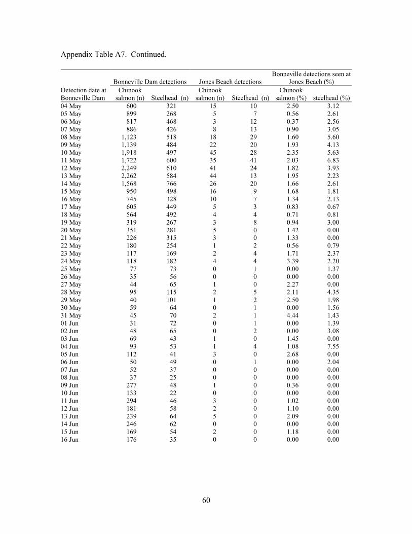
60

Appendix Table A7. Continued.

Detection date at Bonneville Dam

Bonneville Dam detections Jones Beach detections Bonneville detections seen at

Jones Beach (%) Chinook

salmon (n) Steelhead (n) Chinook

salmon (n) Steelhead (n) Chinook

salmon (%) steelhead (%) 04 May 600 321 15 10 2.50 3.12 05 May 899 268 5 7 0.56 2.61 06 May 817 468 3 12 0.37 2.56 07 May 886 426 8 13 0.90 3.05 08 May 1,123 518 18 29 1.60 5.60 09 May 1,139 484 22 20 1.93 4.13 10 May 1,918 497 45 28 2.35 5.63 11 May 1,722 600 35 41 2.03 6.83 12 May 2,249 610 41 24 1.82 3.93 13 May 2,262 584 44 13 1.95 2.23 14 May 1,568 766 26 20 1.66 2.61 15 May 950 498 16 9 1.68 1.81 16 May 745 328 10 7 1.34 2.13 17 May 605 449 5 3 0.83 0.67 18 May 564 492 4 4 0.71 0.81 19 May 319 267 3 8 0.94 3.00 20 May 351 281 5 0 1.42 0.00 21 May 226 315 3 0 1.33 0.00 22 May 180 254 1 2 0.56 0.79 23 May 117 169 2 4 1.71 2.37 24 May 118 182 4 4 3.39 2.20 25 May 77 73 0 1 0.00 1.37 26 May 35 56 0 0 0.00 0.00 27 May 44 65 1 0 2.27 0.00 28 May 95 115 2 5 2.11 4.35 29 May 40 101 1 2 2.50 1.98 30 May 59 64 0 1 0.00 1.56 31 May 45 70 2 1 4.44 1.43 01 Jun 31 72 0 1 0.00 1.39 02 Jun 48 65 0 2 0.00 3.08 03 Jun 69 43 1 0 1.45 0.00 04 Jun 93 53 1 4 1.08 7.55 05 Jun 112 41 3 0 2.68 0.00 06 Jun 50 49 0 1 0.00 2.04 07 Jun 52 37 0 0 0.00 0.00 08 Jun 37 25 0 0 0.00 0.00 09 Jun 277 48 1 0 0.36 0.00 10 Jun 133 22 0 0 0.00 0.00 11 Jun 294 46 3 0 1.02 0.00 12 Jun 181 58 2 0 1.10 0.00 13 Jun 239 64 5 0 2.09 0.00 14 Jun 246 62 0 0 0.00 0.00 15 Jun 169 54 2 0 1.18 0.00 16 Jun 176 35 0 0 0.00 0.00

61

Appendix Table A7. Continued.

Detection date at Bonneville Dam

Bonneville Dam detections Jones Beach detections Bonneville detections seen at

Jones Beach (%) Chinook

salmon (n) Steelhead (n) Chinook

salmon (n) Steelhead (n) Chinook

salmon (%) steelhead (%) 17 Jun 155 24 0 0 0.00 0.00 18 Jun 47 11 0 0 0.00 0.00 19 Jun 55 14 1 0 1.82 0.00 20 Jun 58 10 1 0 1.72 0.00 21 Jun 128 11 3 0 2.34 0.00 22 Jun 107 10 0 0 0.00 0.00 23 Jun 67 16 0 0 0 0 24 Jun 50 15 0 0 0 0 25 Jun 119 13 2 0 2 0 26 Jun 187 13 1 0 1 0 27 Jun 241 8 3 0 1 0 28 Jun 179 6 2 0 1 0 29 Jun 146 3 1 0 1 0 30 Jun 229 6 0 0 0 0 01 Jul 434 5 0 0 0 0 Totals 30,950 12,909 398 334 1.29 2.59

62

63

APPENDIX B

Detection Efficiency Tests As in previous years, we used a test tape to evaluate electronic performance of the matrix detection system (Ledgerwood et al. 2005). For efficiency tests during deployment, we positioned a 2.5-cm diameter PVC pipe through the center of both the front and rear component of the matrix antenna. The pipe extended beyond the reading range of the electronic fields (at least 0.5 m) of both the front and rear antenna components. A vinyl-coated tape measure with PIT-tags attached at known spacing intervals and orientations was then passed through the pipe, and detection efficiency was evaluated based on the proportion of tags on the tape that were detected during a single pass (Appendix Figure B1). Appendix Figure B1. Schematic depicting test tags on a vinyl tape measure, threaded

through a PVC pipe in the center of the inner matrix antenna coils to evaluated antenna detection efficiency. PIT tags were oriented at 0 and 45 degrees to the direction of travel and spaced at intervals of 30, 60, and 90 cm.

64

In 2009, we developed an additional procedure to evaluate the matrix antenna in a dry environment. In 2011, dry tests were conducted in an enclosed facility and were similar to in-water tests, except that pulleys mounted to the ceiling were used to guide the test tape through the antenna components. In 2009, we redesigned the test tape to better understand the impact of tag collisions (signal cancelation due to more than one tag energized within the detection field) in order to optimize antenna performance (Appendix Table B1). The redesigned tape was configured with 6 individual groups of 9 tags. Spacing and orientation of tags were the same within each group, but differed between groups. The 6 groups were comprised of tag sets oriented at two different angles relative to the antenna detection field (0 and 45 degrees) with tags sets at each angle spaced 30, 60, and 90 cm apart. Both the first and last tag in each group was omitted from analysis because the spacing before and after these tags was not equal. We expected results from efficiency tests to show greater rates of detection with improved alignment, orientation, and proximity to the electronic field. Accounting for some variation in each of these factors, the tape tests allowed rigorous tests of antenna efficiency. The angles and orientations used on the tape did not reflect those of actual PIT-tagged fish, which generally do not pass through the exact center of the coils but closer to the sides where detection efficiency is much higher. We chose densities and orientations along the tape such that not all tags would be detected, partly because the relative consistency of tape detections helped validate electronic tuning and identified possible problems with the electronics. During tests, we suspended the antenna either underwater or in air, and pulled the test tape back and forth several times. The start time of each pass was recorded, and we used standard PIT-tag software to record detections. Efficiency was calculated as the total number of individual (unique) tags decoded during each pass divided by the total number of tags passed through the antenna. The matrix detection system was evaluated for electronic performance at the beginning of the season, but due to the time and difficulty setting up for in-water tests, we only performed these tests during the season on an as-needed basis. We generally relied on status reports generated by the MiniMon software to evaluate tuning, performance, and the need to conduct tape-tests.

65

Appendix Table B1. Configuration of SST PIT-tags on a vinyl-tape measure used to test antenna performance in 2011.

Position on

tape measure (ft) Orientation (°) Distance from previous

tag (ft)a PIT tag codeb 5 45 0 3D9.1C2CC4AE3F 6 45 1 3D9.1C2CC45A80 7 45 1 3D9.1C2CC42A83 8 45 1 3D9.1C2CC42AAA 9 45 1 3D9.1C2CC8107D 10 45 1 3D9.1C2CC711DF 11 45 1 3D9.1C2CC48B0F 12 45 1 3D9.1C2CC4E48C 13 45 1 3D9.1C2CC47161 21 0 8 3D9.1C2CC43D0C 22 0 1 3D9.1C2CC710F1 23 0 1 3D9.1C2CC4D578 24 0 1 3D9.1C2CC4625D 25 0 1 3D9.1C2CC440E7 26 0 1 3D9.1C2CC46137 27 0 1 3D9.1C2CC7008A 28 0 1 3D9.1C2CC81379 29 0 1 3D9.1C2CC6F306 37 45 8 3D9.1C2CC817E9 39 45 2 3D9.1C2CC4A641 41 45 2 3D9.1C2CC4B83D 43 45 2 3D9.1C2CC4E762 45 45 2 3D9.1C2CC6F1E5 47 45 2 3D9.1C2CC46298 49 45 2 3D9.1C2CC4C92B 51 45 2 3D9.1C2CC4E9E0 53 45 2 3D9.1C2CC43F3B 61 0 8 3D9.1C2CC4D3C5 63 0 2 3D9.1C2CC4CE33 65 0 2 3D9.1C2CC4393C 67 0 2 3D9.1C2CC45743 69 0 2 3D9.1C2CC4DE17 71 0 2 3D9.1C2CC43EB4 73 0 2 3D9.1C2CC713DC 75 0 2 3D9.1C2CC4C630

66

Appendix Table B1. Continued.

Position on tape measure (ft) Orientation (°)

Distance from previous tag (ft)a PIT tag codeb

77 0 2 3D9.1C2CC4EFEB 85 45 8 3D9.1C2CC70808 88 45 3 3D9.1C2CC49929 91 45 3 3D9.1C2CC6F33E 94 45 3 3D9.1C2CC4AF9E 97 45 3 3D9.1C2CC43C37 100 45 3 3D9.1C2CC4634A 103 45 3 3D9.1C2CC44376 106 45 3 3D9.1C2CC4928D 109 45 3 3D9.1C2CC43F3A 117 0 8 3D9.1C2CC4C79D 120 0 3 3D9.1C2CC4B62B 123 0 3 3D9.1C2CC44382 126 0 3 3D9.1C2CC43AA4 129 0 3 3D9.1C2CC43EBE 132 0 3 3D9.1C2CC49BCA 135 0 3 3D9.1C2CC42A98 138 0 3 3D9.1C2CC46225 141 0 3 3D9.1C2CC43DF6 a Distance from previous tag as measured in the direction from 17 to 125 ft b PIT-tags were tested after each antenna evaluation with a hand-held reader and replaced as needed

67

Spacing of Adjacent Tags (cm)30 60 90

100

60

40

20

0

80

Effic

ienc

y (%

)

45 0

Results and Discussion

Antenna Performance Detection Efficiency—Detection efficiencies were positively correlated with spacing between tags, regardless of tag orientation. According to PTAGIS, 96% of the PIT-tagged fish released into the basin for migration in 2011 were tagged with SST tags, which have longer read ranges than the older ST tags (PSMFC 2011). About 94% of trawl detections in 2011 were SST tags, with the remaining 6% evenly split between ST tags and a variety of tag types from new tag manufacturers. We tested detection efficiency using SST tags in 2011. The 6-coil matrix antenna only recorded one test-tag, between both orientations, out of the 504 spaced 30 cm apart (shortest spacing tested, Appendix Figure B2). Appendix Figure B2. Detection rate/read efficiency of the matrix antenna during 2011.

Efficiency was determined by targeting 42 of 54 PIT-tags attached to a vinyl tape and passed through the antenna six times. Various spacing intervals between tags and tag orientations to the electronic field were used. Results reflect the combined performance (42 tag codes per pass × 6 passes = 252 possible detections).

68

When spacing between tags was increased to 60 cm, detection efficiency increased to 87% for tags oriented perpendicular to the electronic field and 92% for tags at a 45-degree angle to the field. For test tags spaced 90 cm apart, reading efficiency increased to 98% for perpendicular tags and 95% for angled tags. Antenna Efficiency—Similar to previous years, reading efficiency tests for the individual antenna coils and for the matrix system overall were conducted in situ prior to sampling operations. The tests are used to evaluate technological ‘upgrades’ and general performance of our system. The tests must be conducted on the weakest part of the antenna field to show any differences. When similar tests are conducted slightly closer to the edges of the antennas (more optimal read area) read efficiencies are nearly 100%. For comparison, the results of these tests are shown with results from earlier tests of the 0.9-m-diameter cylindrical antenna (Appendix Table B2). Appendix Table B2. Comparison of antenna detection efficiencies of a test PIT-tag tape

passed through the 0.9-m diameter cylindrical antenna and the matrix antenna.

Antenna (dimensions) Total tags read (N)

Total tags available (N)

Overall antenna efficiency (%)

Cylindrical (0.9-m diameter) 784 1,176 66.6 Matrix (0.7- × 2.8-m perimeter) 939 1,512 62.1

Although there was a significant gain in volitional fish passage using the larger matrix antenna system (53% more fish detections during simultaneous testing in 2008, Magie et al. 2010), the read efficiency of test tags was 4.5% less than the read efficiency of test tags obtained using the smaller cylindrical antenna system (66.6 to 62.1%). We believe that this slight drop in read efficiency was caused by an increased rate of tag collisions, which was a by-product of the extended read range of SST tags (Figure B2). Tag collision occurs when two or more tags are energized in the detection field and transmit their codes simultaneously, so that neither tag is correctly decoded. Although the older cylindrical antenna had a slightly higher read efficiency with the test tape, the smaller exit to the trawl in the older antenna delayed fish and allowed them more time to escape forward. To test how tag-code collisions affect antenna performance, we conducted laboratory tests with the matrix antenna attempting to reduce the size of the z-axis detection field without compromising field strength (expressed as side-to-side read range, Magie et al. 2011). We were able to do this successfully, but the set-up was not practical for field operations. Tag collision still can occur with the trawl system due to periodic

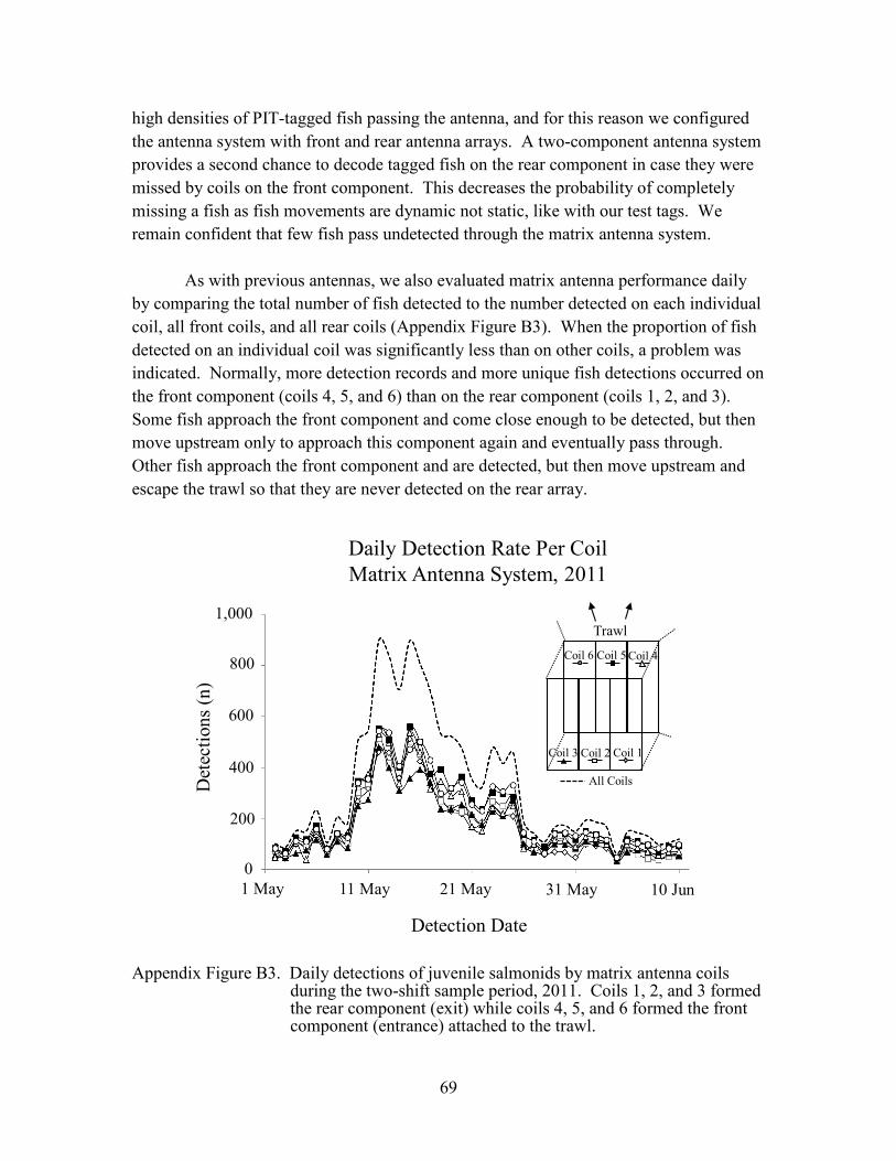
69

Daily Detection Rate Per Coil Matrix Antenna System, 2011

1,000

800

600

400

200

01 May 11 May 21 May 31 May 10 Jun

Detection Date

Det

ectio

ns (n

)

Coil 5 Coil 4Coil 6

Coil 1Coil 2Coil 3

Trawl

All Coils

high densities of PIT-tagged fish passing the antenna, and for this reason we configured the antenna system with front and rear antenna arrays. A two-component antenna system provides a second chance to decode tagged fish on the rear component in case they were missed by coils on the front component. This decreases the probability of completely missing a fish as fish movements are dynamic not static, like with our test tags. We remain confident that few fish pass undetected through the matrix antenna system.

As with previous antennas, we also evaluated matrix antenna performance daily by comparing the total number of fish detected to the number detected on each individual coil, all front coils, and all rear coils (Appendix Figure B3). When the proportion of fish detected on an individual coil was significantly less than on other coils, a problem was indicated. Normally, more detection records and more unique fish detections occurred on the front component (coils 4, 5, and 6) than on the rear component (coils 1, 2, and 3). Some fish approach the front component and come close enough to be detected, but then move upstream only to approach this component again and eventually pass through. Other fish approach the front component and are detected, but then move upstream and escape the trawl so that they are never detected on the rear array. Appendix Figure B3. Daily detections of juvenile salmonids by matrix antenna coils

during the two-shift sample period, 2011. Coils 1, 2, and 3 formed the rear component (exit) while coils 4, 5, and 6 formed the front component (entrance) attached to the trawl.