1

To appear in The International Journal of Intelligent Automation and Soft Computing, 2003

Detection of Welding Flaws with MLP Neural Network and Case Based Reasoning

T. Warren Liao1*, E. Triantaphyllou1, and P.C. Chang2

1Department of Industrial and Manufacturing Systems Engineering

Louisiana State University, Baton Rouge, LA 70803

2Department of Industrial Engineering and Management

Yuan-Ze University, Nei-Li 32026, Chung-Li, Taiwan

Abstract - The correct detection of welding flaws is important to the successful

development of an automated weld inspection system. As a continuation of our previous

efforts, this study investigates the performance of multi-layer perceptron (MLP) neural

networks and case based reasoning (CBR) individually as well as their combined use. It

is found that better performance is attained by all the methods tested in this study than

that was obtained by the fuzzy clustering methods employed before. For each method,

the effect of using different parameters is also investigated and discussed. An

improvement of CBR performance is not guaranteed when the MLP NN based attribute

weighting is used. In addition, none of the three combination-of-multiple-classifiers

methods (majority voting, Borda count, and arithmetic averaging) tested improve the

performance of the best individual classifiers.

Key Words: Welding flaws, MLP neural networks, Case based reasoning, Attribute

weighting, Combination of multiple classifiers

________________________________________________________________________

* Corresponding author. Tel: 225-578-5365; Fax: 225-578-5109; Email: ieliao@lsu.edu

2

1. Introduction

Radiography testing is one of major non-destructive testing (NDT) methods to examine

welds for subsurface flaws. Real-time digital radiography is currently available but more

expensive [Stone et al., 1996]. In most applications, a radiographic weld image is

produced by permitting an X-ray or γ-ray source to penetrate the welded component and

expose a photographic film. In either case, inspection by a certified inspector is needed

with the assistance of a high-resolution monitor or a view box. This manual interpretation

process is often subjective, inconsistent, labor intensive, and biased-prone. There have

been a few attempts to develop computer-aided interpretation systems for identifying

anomalies in welds.

A computer-aided weld quality interpretation system generally has three major

functions: (i) segmentation of welds from the background, (ii) detection of welding flaws

in the weld, and (iii) classification of flaw types. Some of the published work in each one

of these three areas is listed below.

• Segmentation of welds: Liao and Ni [1996], Liao and Tang [1997], and Liao et al.

[2000a].

• Detection of welding flaws: Daum et al. [1987], Gayer et al. [1990], Hyatt et al.

[1996], Liao and Li [1998], and Liao et al. [1999].

• Classification of flaw types: Kato et al. [1992], and Aoki and Suga [1999].

The segmentation of welds from the background is necessary to avoid unproductive

processing of the background where no flaw exists. This is particularly important when

there is more than one weld in the image obtained by scanning more than one films at one

time. Liao and Ni [1996] developed a simple methodology to extract linear welds based

3

on the observation that the intensity profile of a weld is more Gaussian-like than the other

objects in the image. Liao and Tang [1997] presented a three-step procedure for the

automatic extraction of linear as well as curved welds. The three steps are feature

extraction, classification by multi-layer perceptron neural networks, and post processing.

Liao et al. [2000a] modified the above three-step procedure by reducing one feature and

replacing MLP NN classifiers with fuzzy classifiers.

The detection of welding flaws is usually achieved by following three major steps: (i)

preprocessing to remove noise and to increase contrast, (ii) subtracting the test image by

the model of good welds to detect flaws, and (iii) post processing to consolidate the

detected flaws. Previous work differs in the specific algorithms used in each step and

how the model of good welds is constructed.

There are relatively fewer studies on the classification of welding defect types. Kato

et al. [1992] developed an expert system for defect categorization. The rules were

extracted by extensive interviews of inspectors. Ten parameters were used to describe six

types of defects: blowhole, slag inclusion (round), slag inclusion (long), pipe, incomplete

penetration, lack of fusion, and crack. Aoki and Suga [1999] applied a three-layer

feedforward neural network to discriminate five types of defects (blowhole, slag

inclusion, undercut, crack, and incomplete penetration) using ten characteristic values.

The study described in this paper is a continuation of our previous work on the

detection of welding flaws in radiographic weld images. The objective is to devise a

better pattern classification method than the fuzzy clustering methods employed in [Liao

et al., 1999]. This paper shows that case based reasoning (CBR) alone, multi-layer

perceptron neural networks (MLP NN) alone, and the combined use of CBR and MLP

4

NN all yield better performance than that of fuzzy clustering methods. The data used here

is identical to the data used by Liao et al. [1999]. The data set, extracted from

radiographic images of industrial welds, has 10,500 tuples with each tuple having 25

numeric attributes. The categorical (or pattern) value of each record is known, which

indicates whether a particular tuple is a welding flaw (taking a value of 1) or not (0).

Approximately, 14.5% of the tuples represent cases with welding flaws. Please refer to

[Liao et al., 1999] for a more detailed descriptions about these attributes and the

extraction procedure.

The remaining material of this paper is organized as follows: Sections 2 and 3 present

the CBR method and the MLP NN method, respectively. Section 4 describes the

enhancement of CBR with MLP NN based feature weighting. Section 5 studies the

performance of combining the classification outputs derived by individual CBR and/or

MLP NN classifiers. The test results of applying each one of the above methods are

shown and discussed in Section 6. The conclusions are given in the final section.

2. Welding Flaws Detection by Case Based Reasoning

Case-based reasoning (CBR) is one of the emerging paradigms for designing intelligent

systems. It solves new problems by adapting previously successful solutions to similar

problems. Three major issues necessary to be addressed in developing a CBR system

include case representation and organization, case retrieval, and case adaptation.

Each case is usually consisted of two parts:

• problem/situation: a description of the state of the world (i.e., background,

environments and problem descriptions ) when the case happened;

5

• solution: the derived solution or answer to the corresponding problem.

Depending upon the characteristics of the problem domain and the developer's

preference, various forms of representation can be used. They include attribute-value

pairs, frames, objects, predicates, semantic nets and rules. Simple attribute-value pairs

are used to represent each case in this study.

The organization of cases provides a means for accessing individual cases when

searching for a relevant case. Cases should be organized such that retrieval is both

efficient and accurate. Commonly used case organizational structures include flat

structure, feature-based structure, and hierarchical structure. A flat structure is simple

and can be easily implemented as a simple list, an array, or a file. The retrieval of cases

organized in the flat structure is performed by a serial search. Therefore, the retrieval

would be inefficient and expensive as the case base expands. In a feature-based structure,

cases are indexed by chosen key features. Determining key features is thus a crucial step

in this approach. Though improving the efficiency of retrieval to some extent, feature-

based indexing often forms a fixed organization of cases that would not support a flexible

retrieval. A hierarchical structure categories cases from more general features to more

specific features. In addition to the efficiency of retrieval, the hierarchical structure of

case indices can be automatically derived, based on some clustering methods. Because of

the number of cases is relatively small, it is appropriate to employ the simplest flat

structure in this study.

Four commonly used case-retrieval methods are described below.

(1) Template retrieval. SQL-like queries are used to find all cases that satisfy the attached

parameters or conditions. This approach works like a filter, and is often applied

6

before other retrieval approaches, to limit the search space to a more relevant section

of the case base.

(2) K-nearest neighbors (KNN). This is a general classification algorithm for pattern

recognition. In CBR, the algorithm is used to select the K most similar cases, ordered

by the similarity between an old (stored) case and the new (target) case. Based on

these K similar cases, a solution for the target case is provided. Each attribute in the

original KNN approach is equally weighted. A more useful KNN in practice is the

weighted KNN; that is, attributes may have different weights according to their

importance. The general form of similarity measure functions for two cases X and Y

is as follows:

SIM(X,Y) =

∑

∑

=

=×

n

ii

n

iiii

1

1

w

)y,sim(xw, (1)

where n is the number of attributes in a case, wi is the weight of attribute i, and

sim(xi,yj) is the similarity between two values of the same attribute. Due to the

popularity of this retrieval method, CBR systems are sometimes called “similarity-

searching systems”. Liao et al. [1998] studied the similarity-measuring methods and

proposed a hybrid similarity measure to handle both crisp and fuzzy attributes in

CBR. This study employs two most widely used similarity measures based on the

Euclidean distance and Hamming distance. That is,

SIM(X,Y)=

∑−=

),,(-1

,),(11

2

iii

iii

yxdistw

yxdistwn

i (2)

if the Euclidean distance is used

if the Hamming distance is used

7

The weight wi is normalized to denote the importance of the ith attribute. The

normalized dist(xi,yi) is often represented as:

dist(xi, yi) = |xi - yi| / |maxi - mini|, (3)

where xi, yi are the ith attribute values in the two cases. For numerical attributes,

“maxi” and “mini” denote the maximum and minimum values of the ith attributes,

respectively. The major problem in this approach is how to weight the attributes.

Attribute weighting based on MLP NN is discussed in Section 4.

(3) Induction. Induction algorithms such as ID3 [Quinlan, 1979] and k-d trees [Wess et

al., 1994] can be used to identify discriminatory attributes for organizing cases in the

memory into a decision-tree structure.

(4) Knowledge-guided induction. Knowledge is used to guide the induction process

through manually determined case attributes that are thought to be the primary case

features. Because explicit knowledge cannot be obtained easily, this approach is

commonly used together with some other approach(es).

Case adaptation considers the retrieved similar cases partially or all together, and tries

to generate a solution that meets the needs of the target case as close as possible. Some

adaptation methods reviewed by Watson and Marir (1994) are:

(1) Null adaptation that directly applies whatever solution is retrieved without adapting

it. In this study the solution of the most similar case is simply taken as the solution of

the test case because our problem involves simple classification.

(2) Parameter adjustment that compares specified parameters of the retrieved and current

case to modify the solution in an appropriate direction.

(3) Reinstantiation is used to instantiate features of an old solution with new features.

8

(4) Derivational replay uses the method of deriving an old solution to derive a solution

for the new case.

(5) Model-guided repair employs a causal model to guide adaptation.

In general, there are five major steps involved in using a CBR system:

(1) Presentation of a new case.

(2) Retrieval of the most similar cases from the case base.

(3) Adaptation of the selected cases.

(4) Validation of the current solution given by CBR.

(5) Updating of the system by adding the verified solution to the case base.

This procedure is followed, except the last step, to test the CBR system developed for

detecting welding flaws. More details are given in Section 6 when the test results are

presented.

3. Welding Flaws Detection by MLP Neural Networks

The development of the back-propagation (BP) algorithm [Rumelhart et al., 1986] has

revived both the theoretical and practical research of MLP neural networks. It was

theoretically proven that any continuous mapping from a m-dimensional real space to a n-

dimensional real space can be approximated within any given permissible distortion by a

3-layered feedforward neural network with enough intermediate units [Funahashi, 1989;

Hornik et al., 1989; Hornik, 1991]. Numerous successful applications of MLP neural

networks have been reported in function approximation [Liao, 1996, 1998; Liao and

Chen, 1994, 1998], pattern classification [Liao and Tang, 1997], and other applications as

reviewed by Garrett et al. [1993] and Widrow et al. [1994].

9

Specifically, the BrainMaker system developed by California Scientific Software is

used to first establish input-output relationship and then to test unseen data. For training,

BrainMaker uses back-propagation as its engine to modify the connection weights. All

neural models constructed in this study have three layers: the input layer has 25 nodes

corresponding to the 25 numeric attributes, the hidden layer with varying number of

nodes at three levels: 5, 25, and 45, and the output layer with one node corresponding to

the classification. The sigmoid function is used in every node. The criterion used to stop

network training is 500 runs. The percentage of good training data is recorded. A

training datum is considered "good" when the amount of error is within 25% of the

pattern value. Since the pattern range is 1, the training tolerance is set at 0.25. For testing

unseen data, a different criterion is applied. A testing data is declared "good" if the

predicted value differs from the actual value by less than 0.5.

4. Welding Flaws Detection by CBR with MLP NN Based Attribute Weighting

As mentioned in Section 2, the major problem with the KNN based retrieval method is

determining the importance of the attributes. Heuristic-based weighting (decided based

on human knowledge or experience) is commonly applied because of its simplicity.

However, there is no proof that heuristically determined weights are optimal. Sometimes,

the human expert might not feel comfortable in making this decision at all. Due to these

difficulties, researchers have tried to develop automatic attribute weighting methods.

Wettschereck et al. [1997] performed a comprehensive review of attribute weighting

methods by organizing and dichotomizing them along five dimensions:

10

(1) Bias. An attribute weighting method is performance bias if it is guided by feedback

from the classifier and preset bias if it does not incorporate performance feedback.

The weighting methods that incorporate performance feedback were further

distinguished into two groups: those that perform online search in the space of

weights (i.e., sequentially processing each training instance once) and those that

perform batch optimization (i.e., repeatedly pass through the training set). The preset

bias methods were classified into three groups: those based on conditional

probabilities, class projection, and mutual information.

(2) Weight space. This dimension is used to distinguish attribute weighting from attribute

selection algorithms. The latter group are a proper subset of attribute weighting

algorithms that employ binary weights, meaning that the attribute is either retained

(1) or deleted (0).

(3) Representation. This dimension distinguishes algorithms that use the given

representation from those that transform the given representation into one that might

yield better performance.

(4) Generality. A distinction is made for algorithms that learn a single set of weights to

be employed globally (i.e., over the entire instance space) and that learn more than

one set with each to be applied to a local region of the instance space.

(5) Knowledge. This dimension distinguishes algorithms that employ domain specific

knowledge to those that do not.

In addition, they empirically evaluated a subclass of KNN weight learning methods,

primarily on the bias dimension. The results suggested that performance bias methods

are advantageous.

11

∑=

=m

jjjii AwA

1

2)1( ),)((

.))(var()(0

)1(2)2( ∑=

=n

iijijj xwgwA

Most previous studies on attribute weighting for KNN learning algorithms reviewed

above are empirical. Ling and Wang [1997], who computed optimal attribute weight

settings that minimize the predictive errors for 1-NN algorithms performed the first

theoretical work. Under the assumption of uniform distribution of training and testing

examples in a 2-D continuous space, they first derived the average predictive error

introduced by the linear classification boundaries, and used these results to determine the

optimal weights in the 1-NN distance function.

Based on the trained NN and the training data, Shin et al. [2000] derived four

measures called sensitivity, activity, saliency, and relevance to evaluate the importance of

attributes. The last three measures and their average are used here in this study. They are

all detailed below.

Consider a fully connected network with one hidden layer and one output node in the

output layer, as depicted in Fig. 1. There are n+1 inputs with x0 = 1 introduced to include

the bias terms of hidden nodes and xi, i = 1, … , n for input attributes. The hidden layer

has m+1 nodes with z0 = 1 introduced to include the bias term of the output node and zj, j

= 1, … , m for m hidden nodes. Let wji(1) denote a connecting weight from xi to zj, and

wj(2) denote a connecting weight from zj to the output node y.

The activity of an input node xi, labeled as Ai, is defined as

(4)

where Aj denotes the activity of a hidden node zj and is defined as

(5)

In Eq. 5, g(•) is the sigmoid function (=1/(1+e-•) and var(•) is the variance function. In

essence, the activity of a node is measured by the variance of the activation level in the

12

).)()((1

2)2(2)1(∑=

=m

jjjii wwS

∑=

=m

jjjii RwR

1

2)1( ),)((

).var()( )1(2)2(jijj wwR =

training data. The activity of a node is considered to be high when the activation value of

a node is greatly varied. Weights are squared because the variance of linear combination

can be transformed as var(cx) = c2var(x).

The saliency of an input node xi, labeled as Si, is defined as

(6)

This measure of attribute weights is proportional to the squared value of the connection

weights.

The overall relevance of an input node xi, labeled Ri, is defined as

(7)

where Rj is the relevance of a hidden node zj and is defined as

(8)

This measure uses the variance of connection weights into a node as a predictor of the

node's relevance.

The average of the above three measures is also computed as the fourth measure.

Once obtained based on a trained neural network, Ai, Si, Ri, and their average are

alternatively plugged into Eq. 2 for replacing wi for testing the performance.

5. Combination of Multiple Classifiers

There are two basic approaches for combining classifiers: classifier fusion and dynamic

classifier selection. For the classifier fusion approach, individual classifiers are applied

in parallel and their outputs are combined in some manner to achieve a "group

consensus." The dynamic classifier selection approach attempts to predict which single

13

classifier or a selected subset of classifiers is most likely to be correct for a given test

sample. Only the output of the selected classifier(s) is considered in the final decision.

For the former approach, many combining schemes exist. They can be generally

classified into three types corresponding to three different classification results [Xu et al.,

1992]. In the first type each classifier outputs a single class label and these labels are

combined. The majority rule is the simplest example of the first type [Xu et al., 1992].

The Bayesian combining rule operates on the confusion matrix that was derived from the

actual label and the classification label [Foggia et al., 1999]. In the second type the

classifiers output set of class labels ranked in the order of likelihood. The Borda count is

a typical example of the second type [Ho et al., 1994]. The third type involves the

combination of real valued outputs for each class by the respective classifiers. A

conventional example of this type is arithmetic averaging. A more sophisticated

combination method of the third type is based on the Dempster-Shafer theory of evidence

[Ng and Singh, 1998; Rogova, 1994]. Lu and Yamaoka [1997] presented three fuzzy

classification result integration algorithms covering all forms of classification output.

Of interest in this study is whether some of the simple, conventional combination

methods produces better performance than individual classifiers. Consider K individual

classifiers, which were trained using the same training data D = {(xi, yi), i = 1, … , N},

where yi ∈ {C1, … , CM}. For a test sample x, the task of a classifier, say k, is to assign x

a class label, i.e., Lk(x) = Cj, j = 1, … , M, or a numeric vector M(k) = [mk(1), … , mk(M)]t

with mk(j) indicates the degree of confidence for the input pattern being class j. If the

classification output is a numeric vector, the assigned class label can be chosen to be the

14

∑=

=∈=K

kjkj MjCxVxMV

1

,,,1),(maxarg)( L

==∈

otherwiseCxLif

CxV jkj ,0

)(,1)(

∑=

==K

kkj MjjBxBC

1

,,,1),(maxarg)( L

one with the maximum confidence value. Likely, the rank of each class label can be

easily determined by sorting the confidence values.

The combination methods selected for study include majority voting, Borda count,

and arithmetic averaging, as explained below.

5.1. Majority voting

The majority voting method chooses the class most often chosen by different classifiers.

Mathematically, the classification output of the majority voting for a test sample x,

MV(x), is determined as follows:

(9)

where

5.2. Borda count

The final decision of the Borda count method for a test sample x, BC(x) is the class

yielding the largest Borda count. Mathematically,

(10)

where

Bk(j) is the number of classes ranked below the class j by the kth classifier. In the case

that M equals to 2 (i.e., there are only two classes), the class ranked higher will receive a

Borda count of one and the class ranked lower will receive zero Borda count. This special

case makes Eq. 10 exactly equal to Eq. 9.

15

.,,1,)(1maxarg)(1

MjjmK

xAAK

kkj L== ∑

=

5.3. Arithmetic averaging

This method simply chooses the class yielding the maximum of the averaged values of all

individual classifier outputs. Mathematically,

(11)

6. Test Results and Discussion

This section presents the results obtained by applying each one of the four pattern

recognition methods described above. A set of 750 tuples was randomly selected from

the population of 10,500 tuples to serve as the case base for CBR and the training data for

MLP NN. For discussion purpose, the best fuzzy KNN results [Liao et al., 1999] are

noted as follows: 83.15% accuracy, 18.68% false positive or false alarm (non-flaw

mistaken as flaw), and 6.01% false negative or missing (flaw mistaken as non-flaw).

6.1. CBR with equally weighed attributes

According to Section 2, a CBR system was developed for testing. The system contains

750 cases with each represented as a flat list of features (25 inputs and one output). The

case retrieval method is a 5-NN (i.e., K=5). Since only the output of the closest or the

most similar NN is used as the predicted output for the test case here, varying K actually

does not make any difference. The empirical results given in Figs. 2 - 4 confirm this

expectation.

Two tests were performed. The leave-one-out method was followed to test each tuple

of the 750 data used in the case base. In addition, the entire population of 10,500 tuples

16

b

K

bK

iti

tbt sol

S

SSol ⋅= ∑

∑=

=

1

1

was also tested. The results are summarized in Table 1. Comparing with the best fuzzy

KNN results, CBR with equally weighed attributes yields higher accuracy regardless the

distance measure used. The results also indicate that the Hamming distance is preferable

to the Euclidean distance. The normalization of distance measure has negligible effect.

To determine whether the performance will be any different, two case adaptation

methods were also studied. Both methods take all nearest neighbors into consideration.

The first method takes the solution that the majority of nearest neighbors share for the

test case. The second method computes the weighed average of the solutions of all K-

nearest neighbors. Let Stb be the similarity between the new case and old case b and Solb

be the solution of old case b. The predicted solution for the new case, Solt, is calculated

as follows:

(12)

Table 2 shows the results of the above two case adaptation methods when the

Hamming distance was used with K set at 5. Note that only one number is shown

because both methods give exactly the same results. The results indicate that higher

accuracy was achieved for the leave-one-out test but not for the validation test of the

entire population. There is thus no clear advantage of using the two case adaptation

methods.

To determine the effect of K (i.e., the number of nearest neighbors), the performance

of CBR with the Hamming distance was computed by varying K at six levels: 1, 3, 5, 10,

15, and 20. The results are plotted in Figs. 2 - 4 for the accuracy, false positive and false

17

negative percentage, respectively. Based on these results, the following observations can

be made:

• The number of nearest neighbors does not affect the performance if the solution of the

most similar case is taken, as the solution of the test case (i.e., null adaptation).

• For the two case adaptation methods, their performance is identical to the case of no

adaptation when K = 1. As K increases, their performance degrades. This downward

trend was also reported by Shin et al. [2000].

• The adaptation method that computes the weighted average of the solutions of all

nearest neighbors gives equal or better results (high accuracy and low errors) than the

adaptation method that uses the solution that the majority of nearest neighbors share.

6.2. MLP NN

According to Section 3, MLP neural networks with three different numbers of hidden

nodes were trained and tested. Each MLP neural network was trained four times with

different initial connection weights.

Table 3 summarizes the test results. The training and testing results in the table were

based on 675 and 75 tuples (9-to-1 split of 750), respectively. The validation results were

based on the entire population of 10,500 tuples. The results indicate that MLP neural

networks might achieve higher accuracy than fuzzy KNN if appropriate network

topologies are used. Among all the three topologies tested, 25 hidden nodes produce the

best results. Depending upon the initial weights, the best performance of this particular

topology achieves detection accuracy as high as 97.6%, false positive as low as 2.4%, and

false negative of 2.9%. These result tops all other results obtained in this study. Note

18

that for each topology the performance could greatly vary (20% for the topology with 45

hidden nodes) when a different set of initial connection weights is used.

6.3. CBR with MLP NN based attribute weighting

Each trained MLP neural network and the 750 tuples used for its training were used to

compute the attribute weights according to the equations presented in Section 4. The

weight of the highest activity, saliency, and relevance value is taken as one. The weight

of each other value is the ratio of their value over the maximum. The normalized

attribute weights obtained by trained networks initialized by a different set of connection

weights are quite different, as illustrated in Fig. 5. The same pattern holds for other

attribute-weighting measures, computed based on MLP neural networks trained using a

different number of hidden nodes. To save space, these figures are not shown.

Therefore, the average of normalized attribute weights is used throughout this study.

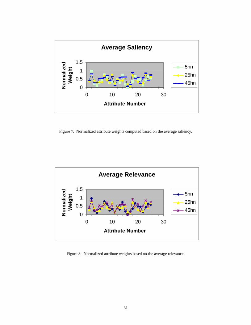
Figures 5 - 8 plot the average normalized attribute weights for activity, saliency, and

relevance, respectively. These plots show the difference in the average normalized

attribute weights when networks were trained using a different number of hidden nodes.

Figures 9 - 11 plot the average normalized attribute weights for three different numbers

of hidden nodes: 5, 25, and 45. These plots show the difference in three different

attribute-weighting measures: activity, saliency, and relevance.

For each topology, attribute weights that were computed for the networks initialized

differently were used to calculate the average attribute weights, which were in turns used

to test the performance. Tables 4-6 summarize the test results for each measure: activity,

saliency, and relevance, respectively. Statistical analyses find that the only significant

19

factor at 5% level is the distance measure. Overall the Hamming distance has a better

performance than the Euclidean distance. There is no significant difference in the

performance as to whether the distance measure is normalized or not and as to how many

hidden nodes are used. Table 7 gives the test results for the average of all three

measures. The same patterns, as observed above for individual measures, seem also to

hold for these results. Comparing with the best fuzzy KNN results, CBR with MLP NN

based attribute weights yields higher accuracy regardless the distance measure and the

trained MLP NN used.

6.4. Combination of classifiers

For a combination-of multiple-classifiers (CMC) method to be of practical use, it should

improve on the best individual classifier, given that the individual classifiers have been

reasonably optimized with regard to parameter settings and available feature data.

Therefore, the CBR classifier with the Humming distance and the MLP NN classifier

with 25 nodes are selected for further study in this section. Each one of the three

combination methods (as explained in Section 5) was tested with three groups of

classifiers. The first group has three CBR classifiers differing only in the case adaptation

method used to derive their classification result. The second group comprises four MLP

NN classifiers differing only in the initial connection weights used in their training. The

third group is consisted of all of the above classifiers.

Table 8 summarizes the test results. These results indicate that: (1) No CMC method

tested produces better performance than the best individual classifier. (2) All CMC

methods have the performance between the best and the worst individual classifiers. (3)

20

The majority-voting method and the Borda count method have equivalent performance.

The last result confirms that Eq. 9 and Eq. 10 are equivalent in the case that M is two. A

more sophisticated combination method is thus called for in order to improve on the

performance of the best individual classifier for the subject application. This will be

investigated further in the future study.

6.5. Comparison of individual classifiers

Based on all the results obtained in this study, the following observations can be made.

First, the performance of CBR is relatively stable regardless the distance measure and the

trained MLP NN used for attribute weighting. On the other hand, the performance of

MLP neural networks is relatively volatile. Thus, one should be more careful when using

MLP neural networks. Unfortunately, there is no theory to guide the configuration of an

optimal MLP neural network for a particular application. Despite the fact that the best

results presented in this paper are given by the 25 × 25 × 1 MLP neural network, it was

obtained only after a fairly extensive trial-and-error effort.

Secondly, the performance of CBR with MLP NN based attribute weighting is not

always better than that of CBR with equally weighed attributes. For the validation of the

set of 10,500 data, CBR with equally weighed attributes dominates in all cases. For the

leave-one-out test of the set of 750 data, CBR with MLP NN based attribute weighting

fair better overall. There is thus no guarantee that MLP NN based attribute weighting will

always produce better results.

21

7. Conclusions

This paper has presented the performance of four popular pattern classification methods

for welding flaws detection using data that were obtained in [Liao et al., 1999]. These

methods including case based reasoning, MLP neural networks, MLP NN based attribute

weighting, and combination of multiple classifiers have found successful applications in

various problem domains. The results obtained in this study indicate that better

performance in terms of higher accuracy rate and lower false positive rate can be

achieved than that of the fuzzy clustering methods employed before. Nevertheless, the

false negative rate is kind of high for most of the methods tested in this study.

Physically, this high false negative rate means many flaws are not detected. In an

application where flaws are detrimental or potentially fatal, such high false negative rate

could be intolerable and costly. Further research is thus needed.

Nevertheless, the following conclusions can be made based on the results of this

study. For the case based reasoning method, the Hamming distance and null adaptation

are preferred. For the MLP neural networks, 25 hidden nodes give the best performance.

The MLP NN based attribute weighting method only improves the performance of the

750 data set based on the leave-one-test, but not the performance of the 10,500 data set.

None of the three methods used to combine individual classifiers (including the majority

voting, the Borda count, and the arithmetic averaging method) improve the performance

of the best individual classifiers. Therefore, another possible future study is to devise a

better combination method.

22

References

1. Aoki, L. and Suga, Y., "Application of Artificial Neural Network toDiscrimination of Defect Type in Automatic Radiographic Testing of Welds",ISIJ International, 39(10), 1999, 1081-1087.

2. Daum, W., Rose, P., Heidt, H., and Builtjes, J. H., "Automatic Recognition ofWeld Defects in X-ray Inspection", British Journal of NDT, 29(2), 1987, 79-82.

3. Foggia, P., Sansone, C., Tortorella, F., and Vento, M., "Multiclassification: rejectcriteria for the Bayesian combiner", Pattern Recognition, 32, 1999, 1435-1447.

4. Funahashi, K., On the approximate realization of continuous mappings by neuralnetworks. Neural Networks, 2, 183-192 (1989).

5. Garrett, J. H., Jr., Case, M. P., Hall, J. W., Yerramareddy, S., Herman, A., Sun,R., Ranjithan, S., and Westervelt, J., "Engineering Applications of NeuralNetworks", Journal of Intelligent Manufacturing, 4, 1993, 1-21.

6. Gayer, A., Saya, A., Shiloh, A., "Automatic Recognition of Welding Defects inReal Time Radiography", NDT International, 23(3), 1990, 131-136.

7. Ho, T. K., Hull, J. J., and Srihari, S. N., "Decision combination in multipleclassifier systems", IEEE Trans. on Pattern Analysis and Machine Intelligence,16(1), 1994, 66-75.

8. Hyatt, R., Kechter, G. E., and Nagashima, S., "A Method for Defect Segmentationin Digital Radiographs of Pipeline Girth Welds", Materials Evaluation, August1996, 925-928.

9. Hornik, K., Stinchcombe, M., and White, H., "Multilayer Feedforward Networksare Universal Approximators", Neural Networks, 2, 359-366 (1989).

10. Hornik, K., "Approximation Capabilities of Multilayer Feedforward Networks",Neural Networks, 4, 251-257 (1991).

11. Kato, Y., Okumura, T., Matsui, S., Itoga, K., Harada, T., Sugimoto, K., Michiba,K., Iuchi, S., and Kawano, S., "Development of an Automatic Weld DefectIdentification System for Radiographic Testing", Weldings in the World, 30(7/8),1992, 182-188.

12. Liao, T. W., "MLP Neural Network Models of CMM Measuring Processes", J. ofIntelligent Manufacturing, 7, 1996, 413-425.

13. Liao, T. W., “Flexural Strength of Creep Feed Ground Ceramics: General Pattern,Brittle-Ductile Transition, and MLP Modeling”, Int. J. Mach. Tools & Manufact.,38(4), 1998, 257-275.

14. Liao, T. W. and Chen, L. J., A Neural Network Approach for Grinding Processes:Modeling and Optimization, Int. J. Mach. Tools & Manufact., 34(7), 1994, 917-937.

15. Liao, T. W. and L. J. Chen, "Manufacturing Process Modeling and OptimizationBased on Multi-Layer Perceptron Networks", ASME Trans. J. of ManufacturingScience and Engineering, 120(1), 1998, 109-119.

16. Liao, T. W., Li, D.-M. and Li, Y.-M., “Extraction of Welds from RadiographicImages Using Fuzzy Classifiers,” Information Sciences, 126, 2000a, 21-42.

17. Liao, T. W., Li, D.-M., and Li, Y.-M., “Detection of Welding Flaws fromRadiographic Images with Fuzzy Clustering Methods”, Fuzzy Sets and Systems,108(2), 1999, 145-158.

23

18. Liao, T. W. and Li, Y.-M., “An Automated Radiographic NDT system for Welds,Part II: Flaw Detection”, NDT&E International, 31(3), 1998, 183-192.

19. Liao, T. W. and Ni, J., "An Automated Radiographic NDT System for Welds,Part I: Weld Extraction", NDT&E International, Vol. 29, No. 3, June 1996, pp.157-162.

20. Liao, T. W. and Tang, K., “Extraction of Welds from Digitized RadiographicImages Based on MLP Neural Networks”, Applied Artificial Intelligence, 11,1997, 197-218.

21. Liao, T. W., Zhang, Z.-M., and Mount C. R., “Similarity Measures for Retrievalin Case Based Reasoning Systems,” Applied Artificial Intelligence, 12(4), 1998,267-288.

22. Liao, T. W., Zhang, Z.-M., and Mount, C. R., “A Case-based ReasoningApproach to Identifying Failure Mechanisms,” Engineering Applications ofArtificial Intelligence, 13(2), 2000b, 199-213.

23. Ling, C. X. and Wang, H., "Computing Optimal Attribute Weight Settings forNearest Neighbor Algorithms", Artificial Intelligence Review, 11, 1997, 255-272.

24. Lu, Y. and Yamaoka, F., "Fuzzy Integration of Classification Results", PatternRecognition, 30(11), 1997, 1877-1891.

25. Ng, G. S. and Singh, H., "Democracy in Pattern Classifications: Combinations ofVotes from Various Pattern Classifiers", AI in Engineering, 12, 1998, 189-204.

26. Quinlan, J. R., "Discovering Rules by Induction from Large Collection ofExamples", in D. Michie (Ed.), Expert Systems in the Microelectronic Ages,Edinburgh University Press, 1979, 169-201.

27. Rogova, G., "Combining the Results of Several Neural Network Classifiers",Neural Networks, 7(5), 1994, 777-781.

28. Rumelhart, D. E., Hinton, G. E., and R. J. Williams, "Learning InternalRepresentation by Error Propagation", Parallel Distributed Processing:Explorations in the Microstructure of Cognition, Vol. 1: Foundations, (edited byD. E. Rumelhart and J. L. McClelland). MIT Press, Cambridge, MA, 1986.

29. Shin, C.-K., Yun, U. T., Kim, H. K., and Park, S. C., "A Hybrid Approach ofNeural Network and Memory-Based Learning to Data Mining", IEEE Trans. onNeural Networks, 11(3), 2000, 637-646.

30. Stone, G. R., Gilblom, D., and Lehmann, D., "100 Percent X-ray WeldInspection: A Real-Time Imaging System for Large Diameter Steel PipeManufacturing", Materials Evaluation, February 1996, 132-137.

31. Watson, I and Marir, F., "Case-based Reasoning: A Review", The KnowledgeEngineering Review, 9(4), 1994, 327-354.

32. Wess, S., Althoff, K.-D., and Derwand, G., "Using k-d Trees to Improve theRetrieval Step in CBR", in S. Wess, K.-D. Althoff and M. M. Richter (Eds.),Topics in Case-Based Reasoning, Springer, 1994, 167-181.

33. Widrow, B., Rumelhart, D. E., and Lehr, M. A., "Neural Networks: Applicationsin Industry, Business and Science", Communications of the ACM, 37(3), 1994,93-105.

34. Xu, L., Krzyzak, A., and Suen, C. Y., "Methods of combining multiple classifiersand their applications to handwriting recognition", IEEE Trans. on Sys. Man.Cybernet., 22(3), 1992, 418-435.

24

Table 1. Performance of CBR with equally weighted features.

750 10500Accuracy False

PositiveFalse

NegativeAccuracy False

PositiveFalse

NegativeNot

normalized93.7% 20.2% 3.9% 94.1% 2.5% 26.2%Euclidean

Normalized 94.0% 3.3% 22.0% 94.2% 2.4% 26.2%Not

normalized94.1% 15.6% 4.2% 94.8% 2.1% 23.8%Hamming

Normalized 94.5% 2.7% 22.0% 94.7% 2.2% 23.8%

Table 2. Performance of two case adaptation methods.

750 10500Accuracy False

PositiveFalse

NegativeAccuracy False

PositiveFalse

NegativeNot

normalized95.1% 7.3% 4.5% 94.0% 1.4% 33.7%Hamming

Normalized 95.1% 1.3% 26.6% 93.9% 1.4% 33.8%

Table 3. Performance of MLP neural networks.

Training Testing Validation# Hiddennodes

Randomseed Accuracy Accuracy Accuracy False

PositiveFalse

Negative1 86.7% 78.7% 73.8% 28.7% 11.2%2 89.3% 85.3% 82.6% 17.4% 17.6%3 89.3% 90.7% 87.7% 10.6% 22.4%4 87.6% 80.0% 74.5% 27.9% 11.0%

5

Avg 88.2% 83.7% 79.7% 21.2% 15.6%1 92.7% 96.0% 89.2% 8.4% 25.1%2 92.0% 92.0% 96.3% 3.1% 7.3%3 93.5% 93.3% 97.6% 2.4% 2.9%4 94.2% 90.7% 96.8% 2.4% 5.7%

25

Avg 93.1% 93.0% 95.0% 4.1% 10.3%1 93.7% 94.7% 90.2% 6.9% 26.9%2 88.2% 88.0% 92.3% 4.3% 28.2%3 93.6% 94.7% 73.0% 17.0% 86.9%4 94.8% 93.3% 93.0% 3.5% 27.3%

45

Avg 92.6% 92.7% 87.1% 7.9% 42.3%

25

Table 4. Performance of CBR with MLP NN attribute weighting by activity.

750 10500DistanceMeasure

Numberof Hidden

NodesAccuracy False

PositiveFalse

NegativeAccuracy False

PositiveFalse

Negative5 93.1% 3.4% 27.5% 93.9% 2.6% 27.1%25 93.5% 3.9% 22.0% 93.3% 3.0% 28.3%

Euclidean -not

normalized 45 94.1% 2.8% 23.9% 93.2% 3.4% 26.9%5 93.3% 3.9% 22.9% 93.7% 2.8% 27.3%25 92.9% 3.3% 29.4% 93.4% 3.2% 27.3%

Euclidean -normalized

45 93.9% 3.6% 21.1% 92.8% 3.7% 28.3%5 95.3% 1.6% 22.9% 94.5% 2.3% 24.4%25 95.2% 1.7% 22.9% 94.5% 2.1% 25.6%

Hamming -not

normalized 45 94.4% 2.5% 20.2% 94.1% 2.7% 25.1%5 94.4% 2.5% 23.9% 94.2% 2.6% 25.0%25 93.2% 2.5% 32.1% 94.4% 2.2% 25.8%

Hamming -normalized

45 94.9% 1.9% 23.9% 94.2% 2.6% 25.1%

Table 5. Performance of CBR with MLP NN attribute weighting by saliency.

750 10500DistanceMeasure

Numberof Hidden

NodesAccuracy False

PositiveFalse

NegativeAccuracy False

PositiveFalse

Negative5 95.3% 2.3% 18.4% 93.6% 3.0% 26.8%25 95.2% 1.6% 23.9% 93.9% 2.2% 26.5%

Euclidean -not

normalized 45 93.3% 3.3% 26.6% 93.0% 3.3% 29.1%5 94.5% 2.8% 21.1% 93.4% 3.1% 27.5%25 93.9% 2.5% 27.5% 93.7% 3.0% 26.4%

Euclidean -normalized

45 95.1% 2.3% 20.2% 93.1% 3.3% 28.1%5 95.2% 2.2% 20.2% 94.1% 2.5% 26.0%25 95.7% 2.0% 17.4% 94.5% 2.2% 25.4%

Hamming -not

normalized 45 94.9% 2.7% 19.3% 94.1% 2.5% 26.2%5 94.8% 1.7% 25.7% 94.1% 2.6% 25.2%25 96.1% 1.4% 18.4% 94.3% 2.4% 25.4%

Hamming -normalized

45 94.9% 1.6% 25.7% 94.3% 2.3% 25.7%

26

Table 6. Performance of CBR with MLP NN attribute weighting by relevance.

750 10500DistanceMeasure

Numberof Hidden

NodesAccuracy False

PositiveFalse

NegativeAccuracy False

PositiveFalse

Negative5 95.5% 2.5% 16.5% 93.6% 3.0% 27.0%25 94.8% 2.3% 22.0% 93.6% 2.8% 27.5%

Euclidean -not

normalized 45 94.4% 2.7% 22.9% 93.3% 3.2% 27.6%5 94.8% 2.7% 20.2% 93.5% 3.1% 27.2%25 94.7% 2.0% 24.8% 93.6% 2.9% 27.3%

Euclidean -normalized

45 94.8% 2.0% 23.9% 93.4% 3.1% 27.2%5 95.6% 2.2% 17.4% 94.3% 2.4% 25.7%25 96.4% 1.6% 15.6% 94.3% 2.2% 26.8%

Hamming -not

normalized 45 95.1% 1.6% 24.8% 94.4% 2.4% 25.2%5 95.1% 1.3% 25.7% 94.1% 2.6% 25.2%25 95.5% 1.7% 21.1% 94.5% 2.2% 24.9%

Hamming -normalized

45 95.2% 1.6% 23.9% 94.2% 2.4% 26.1%

Table 7. Performance of CBR with MLP NN attribute weighting by the average of allthree measures.

750 10500DistanceMeasure

Numberof Hidden

NodesAccuracy False

PositiveFalse

NegativeAccuracy False

PositiveFalse

Negative5 94.5% 2.5% 22.9% 93.7% 2.9% 26.6%25 95.1% 2.5% 19.3% 94.0% 2.6% 25.9%

Euclidean -not

normalized 45 93.6% 3.7% 22.0% 93.1% 3.5% 27.6%5 93.7% 3.1% 24.8% 93.7% 2.9% 26.8%25 93.9% 2.7% 26.6% 93.6% 2.9% 27.2%

Euclidean -normalized

45 95.1% 2.2% 21.1% 93.2% 3.3% 27.8%5 94.5% 1.9% 26.6% 94.3% 2.4% 25.1%25 95.7% 2.2% 16.5% 94.4% 2.2% 26.0%

Hamming -not

normalized 45 94.7% 2.7% 21.1% 94.1% 2.5% 26.5%5 93.7% 2.3% 29.4% 94.4% 2.3% 24.8%25 94.9% 2.3% 21.1% 94.4% 2.2% 25.8%

Hamming -normalized

45 95.5% 1.6% 22.0% 94.2% 2.5% 25.6%

27

Table 8. Performance of three CMC methods.

Accuracy False Positive False NegativeFirst Group Majority Voting 94.0% 1.4% 33.7%

Borda Count 94.0% 1.4% 33.6%Weighted Avg 94.0% 1.4% 33.7%

Second Group Majority Voting 91.6% 5.2% 27.9%Borda Count 91.6% 5.2% 27.9%

Weighted Avg 91.2% 6.3% 23.4%Third Group Majority Voting 93.4% 3.3% 26.4%

Borda Count 93.4% 3.3% 26.4%Weighted Avg 94.0% 2.8% 25.0%

28

y

x0 x1 … xn

Figure 1. A MLP NN with one hidden layer.

Figure 2. Effect of K on the accuracy.

91

92

93

94

95

0 10 20 30

K

Per

cent

age

of

accu

racy

Most similar-Not normalized

Most similar -Normalized

Most frequent -Not normalized

Most frequent -Normalized

Weighted Avg -Not normalized

29

Figure 3. Effect of K on the false positive rate.

Figure 4. Effect of K on the false negative rate.

00.5

1

1.52

2.5

0 10 20 30

K

Flas

e po

sitiv

e %

Most similar-Not normalized

Most similar -Normalized

Most frequent -Not normalized

Most frequent -Normalized

Weighted Avg -Not normalized

010

2030

4050

0 10 20 30

K

Flas

e ne

gativ

e %

Most similar-Not normalized

Most similar -Normalized

Most frequent -Not normalized

Most frequent -Normalized

Weighted Avg -Not normalized

30

Figure 5. Variation of normalized weights.

Figure 6. Normalized attribute weights computed based on the average activity.

Activity Based on 25 Hidden Nodes

0

0.5

1

1.5

0 10 20 30

Attribute Number

Nor

mal

ized

W

eigh

tSeed #1

Seed #2

Seed #3

Seed #4

Average Activity

0

0.5

1

1.5

0 10 20 30

Attribute Number

Nor

mal

ized

W

eigh

t 5hn

25hn

45hn

31

Figure 7. Normalized attribute weights computed based on the average saliency.

Figure 8. Normalized attribute weights based on the average relevance.

Average Saliency

0

0.5

1

1.5

0 10 20 30

Attribute Number

Nor

mal

ized

W

eigh

t 5hn

25hn

45hn

Average Relevance

0

0.5

1

1.5

0 10 20 30

Attribute Number

Nor

mal

ized

W

eigh

t 5hn

25hn

45hn

32

Figure 9. Normalized attributed weights based on MLP neural networks with 5 hidden nodes.

Figure 10. Normalized attribute weights based on MLP neural networks with 25 hidden nodes.

5 Hidden Nodes

0

0.5

1

1.5

0 10 20 30

Attribute Number

Nor

mal

ized

W

eigh

t activity

saliency

relevance

25 Hidden Nodes

0

0.5

1

0 10 20 30

Attribute Number

Nor

mal

ized

W

eigh

t activity

saliency

relevance

33

Figure 11. Normalized attribute weights based on MLP neural networks with 45 hidden nodes.

45 Hidden Nodes

0

0.5

1

1.5

0 10 20 30

Attribute Number

Nor

mal

ized

W

eigh

t activity

saliency

relevance