66

Chapter 5

Detection of Optic Disc and

Macula

5.1 Introduction

An efficient detection of optic disc in colour retinal images is a

significant task in an automated retinal image analysis system. Its

detection is prerequisite for the segmentation of other normal and

pathological features. For instance, the measurement of varying optic

disc to cup diameter ratio is used in the detection sight threatening

disease called glaucoma. The position of optic disc can be used as a

reference length for measuring distances in retinal images, especially

for the location of macula. In case of blood vessel tracking algorithms

the location of optic disc becomes the starting point for vessel tracking.

It also acts as landmark feature in registration of multimodal or

temporal images. Finally, in case of diabetic maculopathy lesions

identification, masking the false positive optic disc region leads to

improvement in the performance of lesion detection.

The attributes of optic disc is similar to attributes of hard

exudates in terms of colour and brightness. Therefore it is located and

removed during the hard exudates detection process, thereby avoiding

false positives. In colour fundus photograph shown in Figure 5.1 optic

disc appears as a bright spot of circular or elliptical shape, interrupted

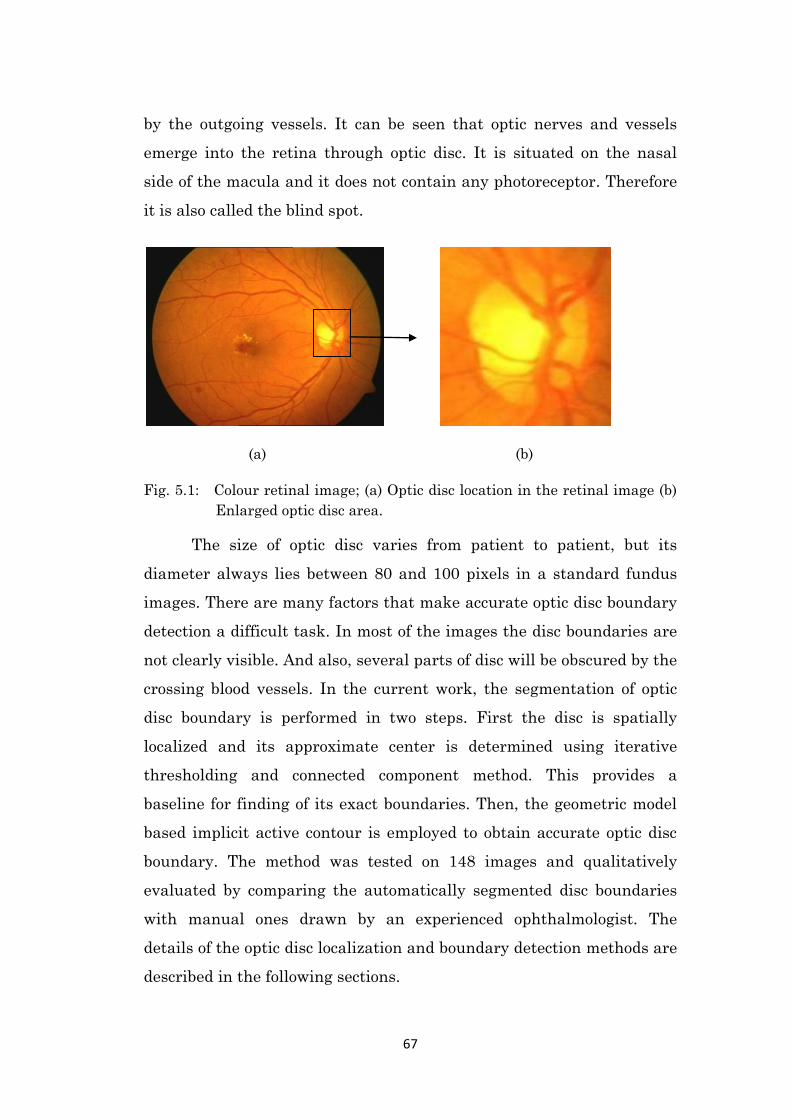
67

by the outgoing vessels. It can be seen that optic nerves and vessels

emerge into the retina through optic disc. It is situated on the nasal

side of the macula and it does not contain any photoreceptor. Therefore

it is also called the blind spot.

(a) (b)

Fig. 5.1: Colour retinal image; (a) Optic disc location in the retinal image (b)

Enlarged optic disc area.

The size of optic disc varies from patient to patient, but its

diameter always lies between 80 and 100 pixels in a standard fundus

images. There are many factors that make accurate optic disc boundary

detection a difficult task. In most of the images the disc boundaries are

not clearly visible. And also, several parts of disc will be obscured by the

crossing blood vessels. In the current work, the segmentation of optic

disc boundary is performed in two steps. First the disc is spatially

localized and its approximate center is determined using iterative

thresholding and connected component method. This provides a

baseline for finding of its exact boundaries. Then, the geometric model

based implicit active contour is employed to obtain accurate optic disc

boundary. The method was tested on 148 images and qualitatively

evaluated by comparing the automatically segmented disc boundaries

with manual ones drawn by an experienced ophthalmologist. The

details of the optic disc localization and boundary detection methods are

described in the following sections.

68

5.2 Localization of Optic Disc

The localization of optic disc is important for two purposes. First, it

serves as the baseline for finding the exact boundary of the disc.

Secondly, optic disc center and diameter are used to locate the macula

in the image. In a colour retinal image the optic disc belongs to the

brighter parts along with some lesions. The central portion of disc is the

brightest region called optic cup, where the blood vessels and nerve

fibers are absent. Applying a threshold will separate part of the optic

disc and some other unconnected bright regions from the background.

In this work an optimal thresholding based on Otsu 1979 method is

applied to separate brighter regions from dark background as follows.

5.2.1 Selection of Initial Threshold

Optimal thresholding method based on approximation of the histogram

of an image using a weighted sum of two or more probability densities

with normal distribution is used for initial thresholding of the retinal

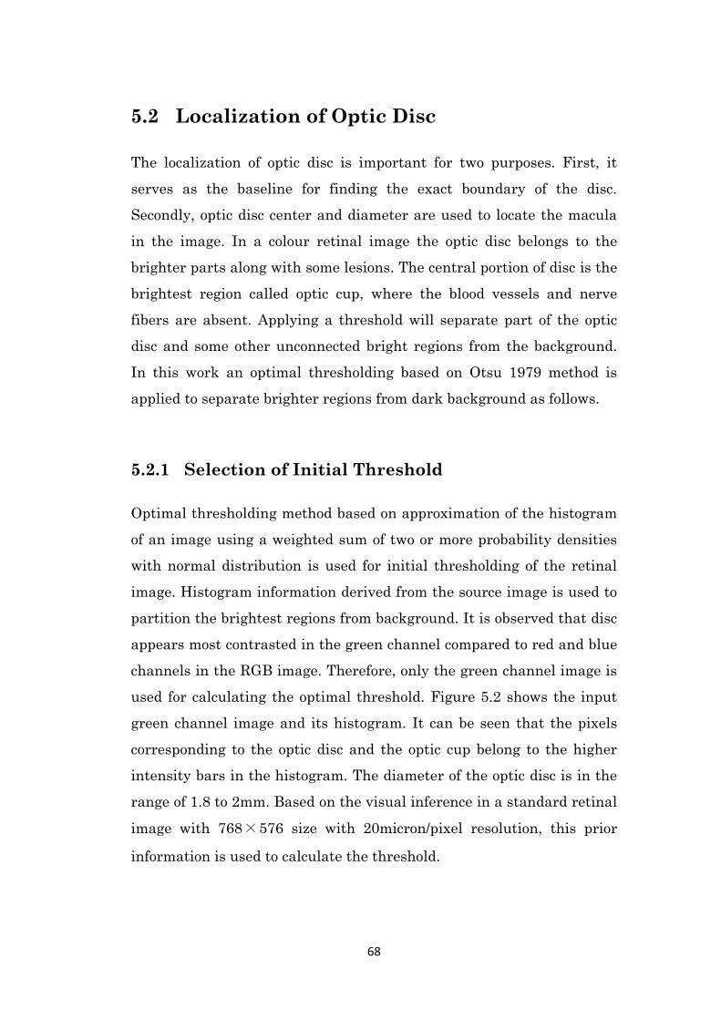
image. Histogram information derived from the source image is used to

partition the brightest regions from background. It is observed that disc

appears most contrasted in the green channel compared to red and blue

channels in the RGB image. Therefore, only the green channel image is

used for calculating the optimal threshold. Figure 5.2 shows the input

green channel image and its histogram. It can be seen that the pixels

corresponding to the optic disc and the optic cup belong to the higher

intensity bars in the histogram. The diameter of the optic disc is in the

range of 1.8 to 2mm. Based on the visual inference in a standard retinal

image with 768×576 size with 20micron/pixel resolution, this prior

information is used to calculate the threshold.

69

(a) (b)

Fig. 5.2: Selecting an optimal threshold; (a) Gray scale of green channel

retinal image; (b) Corresponding histogram with initial threshold.

To obtain an optimal threshold, histogram derived from the

source image I is scanned from highest intensity value l2 to lower

intensity value. The scanning stops at the intensity level l1 which has

atleast a thousand pixels with the same intensity. The initial threshold

Tk for step k=1 is taken as the mean of t2 and t1 resulting in subset of

histograms. Formulation for the calculation of optimal threshold is

given by the following pseudo code.

1. Initial estimate of is calculated at step k as

2. At step k, apply the threshold . This will produce two groups of pixels:

Go consisting of all pixels belonging to object region and Gb consisting

of all pixels belonging to background region.

3. Compute the average intensity values and

for the pixels in Go

and Gb respectively.

4. Update the threshold as follows:

70

5. Repeat steps 2 through 4 difference in T in successive iterations is smaller

than a predefined value.

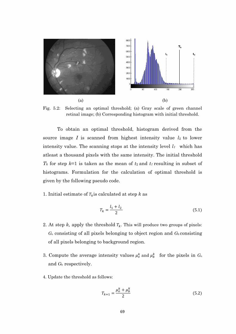
Optimal threshold thus calculated results in maximization of gray level

variance between object and background. Figure 5.3 shows the result of

thresholding on one of the test image resulting in number of isolated

connected regions.

(a) (b)

Fig. 5.3: Optimal thresholding of retinal image; (a) Input colour retinal image;

(b) Thresholded image with number of connected regions.

5.2.2 Estimation of the Optic Disc Center

Thresholding of an image results in number of connected components

such as part of optic disc, some noise and other bright features. These

connected components are candidate regions for optic disc. The entire

image is scanned to count the number of connected components. Each of

the connected components in the thresholded image is labeled, total

number of pixels in the component and mean spatial coordinates of each

connected component is calculated. The component having the

maximum number of pixels is assumed to be having the optic cup part

of disc and it is considered to be the primary region of interest. The

maximum diameter of optic disc can be of 2mm. Therefore, in an image,

if any of the components whose mean spatial coordinates are within 50

pixels distance from the mean spatial coordinates of the largest

71

component, then they are merged with it and new mean spatial

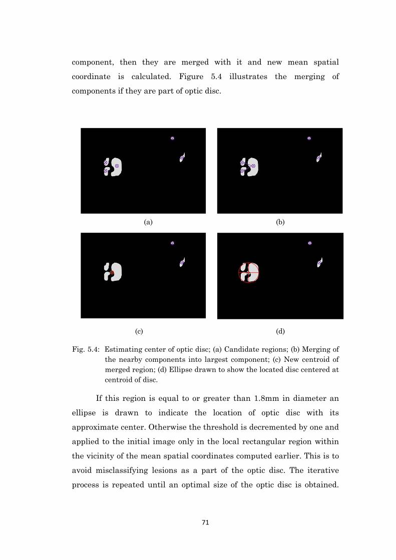
coordinate is calculated. Figure 5.4 illustrates the merging of

components if they are part of optic disc.

(a) (b)

(c) (d)

Fig. 5.4: Estimating center of optic disc; (a) Candidate regions; (b) Merging of

the nearby components into largest component; (c) New centroid of

merged region; (d) Ellipse drawn to show the located disc centered at

centroid of disc.

If this region is equal to or greater than 1.8mm in diameter an

ellipse is drawn to indicate the location of optic disc with its

approximate center. Otherwise the threshold is decremented by one and

applied to the initial image only in the local rectangular region within

the vicinity of the mean spatial coordinates computed earlier. This is to

avoid misclassifying lesions as a part of the optic disc. The iterative

process is repeated until an optimal size of the optic disc is obtained.

72

The following Figure 5.5 illustrates the optic disc localization through

iterative process and its center estimation.

(a) (b)

(c) (d)

(e) (f)

Fig. 5.5: Localization of optic disc; (a) Input colour retinal image; (b) Initial

thresholding; (c)-(e) Detection phase; (f) Ellipse drawn to show

location of optic disc.

73

5.3 Optic Disc Boundary Detection

Glaucoma is the second most common cause of blindness worldwide

(Quigley 1996). It is characterized by elevated Intra Ocular Pressure

(IOP), which leads to damage of optic nerve axons at the back of the eye,

with eventual deterioration or loss of vision. Progression of glaucoma is

slow and silent leading to changes in the shape and size of the optic

disc. Therefore, assessment of optic disc size is an important component

of the diagnostic evaluation for glaucoma. This has led to the motivation

for the accurate detection of optic disc boundary as it is used to detect

and measure the severity of disease.

Difficulty in finding the optic disc boundary is due to its highly

variable appearance in retinal images. Classical segmentation

algorithms such as edge detection, thresholding, and region growing are

not enough to accurately find boundary of the optic disc as they do not

incorporate the edge smoothness and continuity properties. In contrast,

active contour model represent the paradigm that the presence of an

edge depends not only on the gradient at a specific point but also on the

spatial distribution (Kass et al., 1987). Active contours incorporate the

global view of edge detection by assessing continuity and curvature,

combined with the local edge strength thus providing smooth and closed

contours as segmentation results. These properties make them highly

suitable for the optic disc boundary detection application. Active

contours are energy minimizing splines and are generally classified as

parametric or geometric according to their representation. In the

proposed work, the automatic optic disc boundary is detected by fitting

an implicit active contour based on geometric model as reported in Li et

al. 2007. Geometric based model differ from parametric models in the

sense that they do not depend much on image gradient and are less

sensitive to location of initial contour, thus performs better for object

74

with weak boundaries as in case of optic disc. The following sections

provide the details of optic disc boundary segmentation using geometric

active contours.

5.3.1 Elimination of Vessels

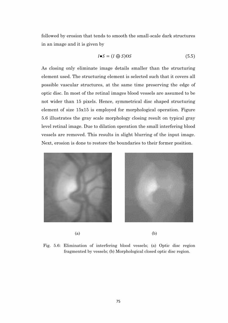
The optic disc region is usually fragmented into multiple sub-regions by

blood vessels that have comparable gradient values. A homogeneous

optic disc region is needed for segmentation using geometric active

contour algorithm. Use of median filter with appropriate size to remove

interfering blood vessels from the optic disc region resulted in heavy

blurring of disc boundaries. Instead a better result is achieved with

gray level mathematical morphology to remove irrelevant vessels from

the optic disc region.

Gray scale mathematical morphology provides a tool for

extracting geometric information from gray scale images. A structuring

element is used to build an image operator whose output depends on

whether or not this element fits inside a given image. Shape and size of

the structuring element is chosen in accordance with the segmentation

task. The two fundamental morphological operations are dilation and

erosion. Denoting an image by I and structuring element by S, the

dilation ⊕ and erosion Ө at a particular pixel (x, y) are defined as:

⊕

[ ]

Ө

[ ]

where i and j index the pixels of S. The opening of an image is defined

as erosion followed by dilation. It tends to smooth the small-scale bright

structures in an image. The closing of an image is defined as dilation

75

followed by erosion that tends to smooth the small-scale dark structures

in an image and it is given by

⊕ Ө

As closing only eliminate image details smaller than the structuring

element used. The structuring element is selected such that it covers all

possible vascular structures, at the same time preserving the edge of

optic disc. In most of the retinal images blood vessels are assumed to be

not wider than 15 pixels. Hence, symmetrical disc shaped structuring

element of size 15x15 is employed for morphological operation. Figure

5.6 illustrates the gray scale morphology closing result on typical gray

level retinal image. Due to dilation operation the small interfering blood

vessels are removed. This results in slight blurring of the input image.

Next, erosion is done to restore the boundaries to their former position.

(a) (b)

Fig. 5.6: Elimination of interfering blood vessels; (a) Optic disc region

fragmented by vessels; (b) Morphological closed optic disc region.

76

5.3.2 Boundary Detection Using Geometric Active

Contour Model (ACM)

In geometric deformation model the curves are evolved implicitly using

geometric computations. The evolving curve is represented as level set

function in the image domain Ω. Image segmentation is performed by

starting with initial curve and evolving its shape by minimizing energy

function represented by level set function. The curve evolution has to

stop at the image boundaries where the energy is minimum. Here, a

contour is represented by zero level set function and the energy

function that is to be iteratively minimized to find the object boundary

is given as follows.

Where is the external energy function, is the zero level set

representing contour C in the image domain, and are two values

that fit the image intensities inside and outside the contour

respectively. is the distance regularizing term used to penalize the

deviation of level set from a signed distance function. It is given by

∫

| |

is the length of zero level curve of used to regularize the contour.

It is given by

∫ | |

and are positive constants, is the smoothing function called dirac

function.

The energy functional (5.6) is to be minimized to find the optic disc

boundary. The gradient descent method proposed by Li et al., 2007 is

used to minimize the energy function and it is given as follows:

77

(

| |) ( (

| |))

The functions and are calculated as follows

∫ | |

∫ | |

where and are positive constants, is the gaussian kernel with

localization property with σ as scaling parameter. and are two

values that fit the image intensities inside and outside the contour. The

first term equation 5.7 is called data fitting term responsible for driving

the active contour toward object boundary. Second term is called length

term and it has smoothing effect on contour. Third term is the level set

regularization term that controls the speed of contour. Large value of σ

can be used if intensity inhomogeneity is not severe. But it increases

the computation time with less iterations required for convergence of

active contour to boundary. Increasing the value of v introduces

emergence of new contours at boundaries of unwanted structures.

Therefore, values of , , , and σ are selected after proper

experimentation for the smooth convergence of the active contour to the

desired disc boundary.

Once the vascular structures are removed based on the gray scale

morphological closing operation, the boundary detection operation is

carried out. To fit active contour onto the optic disc the initial contour

must be near to the desired boundary otherwise it can converge to the

unwanted regions. In order to automatically position an initial contour,

the approximate center of optic disc obtained in the localization method

is used. A set of points whose distance from the center of optic disc is 50

78

pixels more than its disc radius are selected. The contour drawn using

these points becomes the starting point of the curve. Number of

iterations required to detect the boundary of optic disc varies from

image to image. In some images only hundred iterations are enough

and in some more than hundred iterations are needed. Figure 5.7 shows

the convergence of active contour for two different images.

Fig. 5.7: Convergence of active contour towards optic disc boundary in two

different images; (First row) Initial active contour; (Second row)

Active contour after 40 iterations; (Third row) Contour after 150

iterations.

79

(a) (b)

(c) (d)

(e) (f)

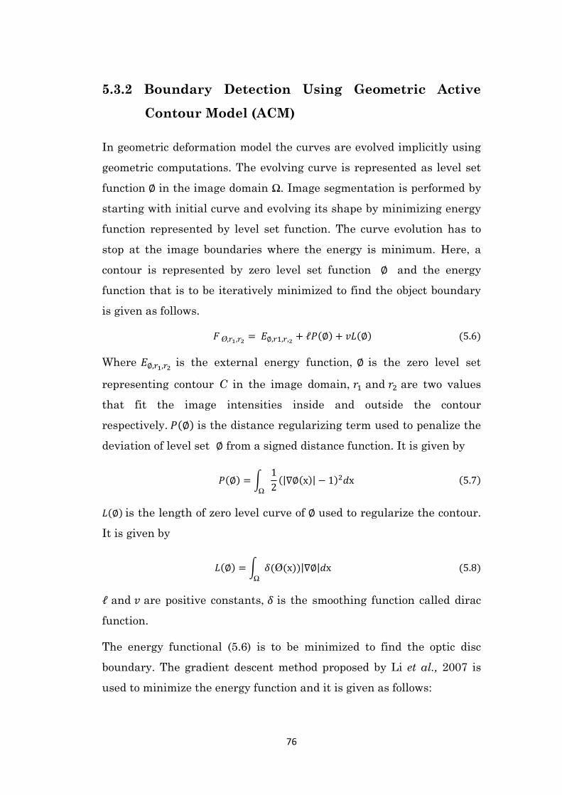
Fig. 5.8: Geometric active contour based optic disc boundary segmentation; (a)

Hand labeled disc boundary of first image; (b) Hand labeled disc

boundary of second image; (c)–(d) Automatically detected boundaries

(green colour) overlapped on corresponding hand labeled images; (e)

Segmented optic disc boundary with 85% sensitivity; (f) Segmented

optic disc boundary with 90.78% sensitivity.

80

Thus obtained contour specifying the boundary of optic disc is further

processed by dilating it with a small structuring element to avoid

discontinuities in the contour. The boundary thus detected is compared

with the manually marked optic disc boundary by an expert and results

are quantified. Figure 5.8 shows the hand labeled optic disc boundary

by an expert and automatically detected optic disc boundary overlapped

on the ground truth image in different colour.

5.4 Detection of Macula

The macula is a depression in the center of macular region and appears

as a darker area in a colour retinal image. It is located temporal to the

optic disc and has no blood vessels present in its center. The fovea

centralis lies at the center of the macula that is utilized in activities

that require discerning sharp details such as reading. Abnormalities

such as exudates present in this region indicate a potential sight

threatening condition called maculopathy. The patient may not be

aware of the presence of the abnormalities if they are small, but, if left

untreated, it results in severe loss of vision. Therefore, it becomes

important to detect and mark the macular region in a retinal image for

automated detection of abnormalities and their severity level.

In a retinal image, the contrast of macula is often quite low and

sometimes it may be obscured by presence of exudates or hemorrhages

in its region. As a consequence a search to obtain a global correlation

often fails. Therefore, the macula is localized based on its distance and

position with respect to the optic disc as it remains relatively constant.

The process of detecting the approximate center and diameter of the

optic disc has been explained in the earlier sections. Once the optic disc

is detected, the macula is localized by finding the darkest region within

81

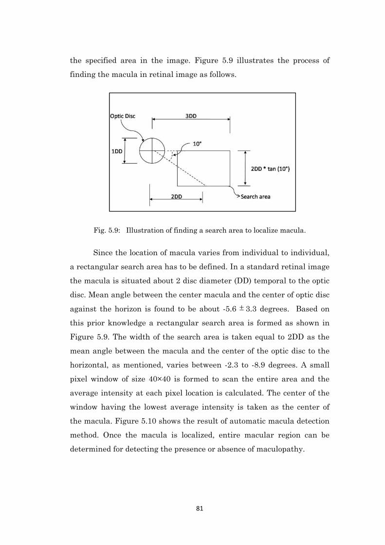
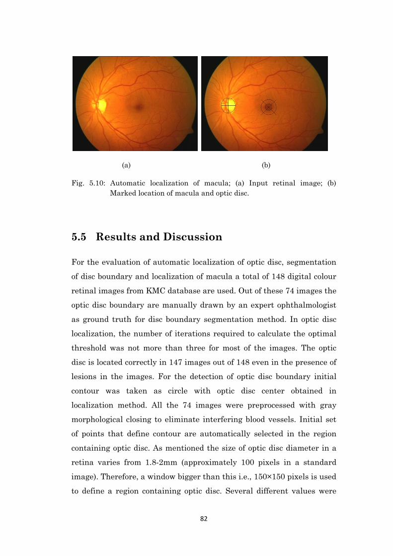
the specified area in the image. Figure 5.9 illustrates the process of

finding the macula in retinal image as follows.

Fig. 5.9: Illustration of finding a search area to localize macula.

Since the location of macula varies from individual to individual,

a rectangular search area has to be defined. In a standard retinal image

the macula is situated about 2 disc diameter (DD) temporal to the optic

disc. Mean angle between the center macula and the center of optic disc

against the horizon is found to be about -5.6 3.3 degrees. Based on

this prior knowledge a rectangular search area is formed as shown in

Figure 5.9. The width of the search area is taken equal to 2DD as the

mean angle between the macula and the center of the optic disc to the

horizontal, as mentioned, varies between -2.3 to -8.9 degrees. A small

pixel window of size 40×40 is formed to scan the entire area and the

average intensity at each pixel location is calculated. The center of the

window having the lowest average intensity is taken as the center of

the macula. Figure 5.10 shows the result of automatic macula detection

method. Once the macula is localized, entire macular region can be

determined for detecting the presence or absence of maculopathy.

82

(a) (b)

Fig. 5.10: Automatic localization of macula; (a) Input retinal image; (b)

Marked location of macula and optic disc.

5.5 Results and Discussion

For the evaluation of automatic localization of optic disc, segmentation

of disc boundary and localization of macula a total of 148 digital colour

retinal images from KMC database are used. Out of these 74 images the

optic disc boundary are manually drawn by an expert ophthalmologist

as ground truth for disc boundary segmentation method. In optic disc

localization, the number of iterations required to calculate the optimal

threshold was not more than three for most of the images. The optic

disc is located correctly in 147 images out of 148 even in the presence of

lesions in the images. For the detection of optic disc boundary initial

contour was taken as circle with optic disc center obtained in

localization method. All the 74 images were preprocessed with gray

morphological closing to eliminate interfering blood vessels. Initial set

of points that define contour are automatically selected in the region

containing optic disc. As mentioned the size of optic disc diameter in a

retina varies from 1.8-2mm (approximately 100 pixels in a standard

image). Therefore, a window bigger than this i.e., 150×150 pixels is used

to define a region containing optic disc. Several different values were

83

tested for the parameters of the gradient descent flow equation and it

was found the weights =0.5, =0.5 that are integrals over the region

outside and inside contour as the best for the retinal images. If

then it resulted in contour being pulled outwards and if reversed then

the contour would converge to regions within optic disc. Value for the

length shortening term v was chosen empirically as 66. Increasing the v

resulted in smooth convergence of contour towards disc boundary, but,

at the cost of increase in the number of iterations. Scaling parameter

was σ was set to 2.0 as in some images the optic disc region had

intensity inhomogeneity. And the regularization value ℓ was set to 1.

The number of iterations for convergence of active contour varied from

120 to 200 for different images. Therefore the iteration was set to 200.

With these parameter settings the geometric active contour algorithm

was applied to 74 images in the dataset. The results were quantified by

comparing the segmented disc boundary against the hand labeled

ground truth images. Sensitivity is used as the measure to match

between two regions in the images. The number of true negatives, that

is, the number of pixels not classified as optic disc region pixels, either

by human expert or by algorithm is very high. This results in specificity

always closer to 100%, that is not meaningful and hence, it is not

considered for evaluating the methods. Identification results are

summarized in Table 5.1. All the algorithms were realized using Matlab

7.0 running on 1.66GHz Intel PC with 1.5GB RAM. And the time taken

to detect the optic disc boundary and macula was less than 30 seconds

with average sensitivity of 90.67±5.05 for optic disc boundary detection

and sensitivity of 96.6% for macula localization.

84

Table 5.1: Performance of optic disc localization, macula localization and

optic disc boundary detection methods

No. of images Method Sensitivity (%)

148 Optic disc

localization 99.32

148 Macula

localization 96.6

74

Optic disc

boundary

detection

90.67±5.05

5.6 Summary

In this Chapter, efficient methods for the automatic segmentation of

optic disc localization, boundary detection and macula localization in

colour retinal images are described. Retinal images of patients at

different stages of retinopathy were considered to test the robustness of

the optimal iterative threshold method followed by connected

component analysis in disc localization. In all the images except one the

optic disc was located correctly. Localization of disc is important as it

has to be masked during the exudates detection and its position is used

in the location of macula. Based on the result obtained in optic disc

boundary detection, it can be stated that geometric based implicit active

contour models provide a better segmentation for images with weak

boundaries when compared to parametric models. Shape and size

changes in optic disc boundaries can be further studied for the detection

of glaucoma. The detection of macula and its region plays an important

role in the severity level classification of diabetic maculopathy.

Detection of all these features leads towards the development of a fully

automated retinal image analysis system to aid clinicians in detecting

and diagnosing retinal diseases.