Detection of High-Latitude Ionospheric Irregularities from GPS Radio Occultation
168
UCGE REPORTS Number 20310 Department of Geomatics Engineering Detection of High-Latitude Ionospheric Irregularities from GPS Radio Occultation (URL: http://www.geomatics.ucalgary.ca/graduatetheses) by Man Feng May 2010
Transcript of Detection of High-Latitude Ionospheric Irregularities from GPS Radio Occultation

UCGE REPORTS
Number 20310
Department of Geomatics Engineering
Detection of High-Latitude Ionospheric Irregularities
from GPS Radio Occultation
(URL: http://www.geomatics.ucalgary.ca/graduatetheses)
by
Man Feng
May 2010

UNIVERSITY OF CALGARY
Detection of High-Latitude Ionospheric Irregularities from GPS Radio Occultation
by
Man Feng
A THESIS
SUBMITTED TO THE FACULTY OF GRADUATE STUDIES
IN PARTIAL FULFILMENT OF THE REQUIREMENTS FOR THE
DEGREE OF MASTER OF SCIENCE
DEPARTMENT OF GEOMATICS ENGINEERING
CALGARY, ALBERTA
May, 2010
© Man Feng 2010

II
ABSTRACT
GPS radio occultation techniques (RO) are effective tools to study ionospheric
layered structures. Electron density is estimated from L1 and L2 excess phase delays
of the RO signal. Ionospheric structures of electron density irregularities can cause
signal fluctuations on GPS L1 and L2 phase paths between the LEO and GPS satellite.
The retrieved electron density profiles and their fluctuations can be studied to gain
new insight into variations and vertical distributions of ionospheric structures in the
high latitude ionosphere for different levels of ionospheric activity, such as
storm-enhanced density (SED) and auroral substorms. In this research high latitude
scintillation effects and associated electron density profiles are analyzed using
COSMIC and CHAMP radio occultation observations. Mechanisms for ionospheric
scintillations are investigated from analysis of fluctuations observed in the retrieved
electron density profiles during the selected disturbed periods. Electron density maps
are also generated to capture the latitudinal extent of the auroral oval under disturbed
ionospheric conditions.

III
ACKNOWLEDGEMENTS
I would like to take this opportunity to thank everyone that helped and supported me
to complete the research during the two and half years.
First and foremost, To Dr. Susan Skone, I would like to sincerely thank you for
providing me the great opportunity to pursue my graduate study in Department of
Geomatics Engineering. Thank you for your helps, patient guidance, and continuous
support. You inspire my exploration of both ionosphere science and geomatics
engineering. You teach me to think in an academic manner. You also lead me to the
gate of research and make me really enjoy the time of working with you.
To Dr. Yang Gao, Dr Kyle O’Keefe, Dr. Geard Lachapelle and Dr. Naser El-Sheimy
thank you for your various help and instruction to me through my study.
To other members of Dr. Susan Skone’s group, Ossama, Fatemeh, Rajesh and
Sadeque thanks for being so analytical and for letting me interrupt you as often as I
did to get help from you.
To my family, my dear father and mother, thanks for caring about me and supporting
me throughout my entire life. Thanks for all the encouragement and comfort from you
when I met difficulties. Thanks for the endless love from my family.

IV
TABLE OF CONTENTS
Abstract ........................................................................................................................ ii
Acknowledgements ...................................................................................................... iii
Table of Contents .......................................................................................................... iv
List of Tables ...............................................................................................................vii
List of Figures ............................................................................................................ viii
List of Abbreviations ................................................................................................. xiii
CHAPTER 1: INTRODUCTION ............................................................................... 1
1.1 Background ....................................................................................................... 1
1.1.1 Review of radio occultation techniques for ionosphere observations .......... 5
1.2 Objectives ......................................................................................................... 7
1.3 Outline............................................................................................................... 8
CHAPTER 2: INTRODUCTION TO GPS THEORY ................................................ 11
2.1 Overview of global positioning system ............................................................. 11
2.1.1 Space segment ............................................................................................. 12
2.1.2 Control segment .......................................................................................... 13
2.1.3 User segment ............................................................................................... 13
2.2 GPS signal description ....................................................................................... 14
2.3 GPS error sources............................................................................................... 17
2.4 GPS modernization ............................................................................................ 19
CHAPTER 3: IONOSPHERIC EFFECTS ON GPS ................................................... 21
3.1 Ionosphere introduction ..................................................................................... 21
3.1.1 Regions of the ionosphere ........................................................................... 22
3.2 High latitude ionosphere .................................................................................... 25
3.2.1 Magnetic field ............................................................................................. 25
3.2.2 High latitude ionospheric irregularities ...................................................... 26
3.2.2.1 Auroral oval ..................................................................................... 27
3.2.2.2 Polar cap .......................................................................................... 29
3.2.3 Ionospheric phenomena .............................................................................. 29
3.3 Ionosphere impact on GPS/GNSS signals ......................................................... 31
3.3.1 First order effect ........................................................................................ 32
3.3.1.1 TEC measurement .......................................................................... 34
3.3.2 Scintillation effects ................................................................................... 35
3.3.2.1 Scintillation theory ......................................................................... 35
3.3.2.2 Global morphology of ionospheric scintillaitons ........................... 36
3.3.2.3 Scintillation measurements ............................................................ 38
3.3.2.4 Phase cycle slips ............................................................................. 39
3.3.2.5 GPS positioning error ..................................................................... 41
3.3.2.6 Fluctuation of radio occultation signal SNR .................................. 43

V
CHAPTER 4: RADIO OCCULTATION TECHNIQUE ......................................... 45
4.1 Overview of radio occultation technique ........................................................... 45
4.2 CHAMP and COSMIC missions ....................................................................... 47
4.2.1 CHAMP ...................................................................................................... 47
4.2.2 COSMIC ..................................................................................................... 50
4.2.3 Comparision between CHAMP and COSMIC ........................................... 53
4.3 Radio occultation data processed by CDAAC ................................................... 55
4.3.1 Algorithms for radio occultation inversions in the ionosphere ................... 56
4.3.1.1 Abel inversion .................................................................................. 57
4.3.1.2 Inversion using slant TEC measurements ........................................ 53
CHAPTER 5: VALIDATION OF RADIO OCCULTATION OBSERVATIONS BY
GROUND OBSERVATIONS ..................................................................................... 62
5.1 Ground observations .......................................................................................... 62
5.1.1 Scintillation observations ............................................................................ 62
5.1.2 Magnetometer observations ........................................................................ 63
5.1.3 Incoherent scatter radar ............................................................................... 65
5.2 Validation by incoherent scatter radar ............................................................... 66
5.2.1 Published validation .................................................................................... 66
5.2.2 Validation under disturbed conditions ........................................................ 68
5.2.2.1 Comparison with incoherent scatter radar observations.................. 68
5.3 Validation by ionosonde .................................................................................... 72
5.4 Validation summary ........................................................................................... 74
CHAPTER 6: CHARACTERISTICS OF RADIO OCCULTATION
OBSERVATIONS UNDER DISTURBED IONOSPHERIC CONDITIONS ............ 76
6.1 Methodology ...................................................................................................... 76
6.1.1 Detrending method description ................................................................... 77
6.1.2 General characteristics of auroral events .................................................... 78
6.1.2.1 Low frequency observations ............................................................ 78
6.1.2.2 High frequency observations ........................................................... 81
6.1.3 Data processing ........................................................................................... 83
6.1.4 Auroral boundary prediction ....................................................................... 86
6.1.5 Events selection .......................................................................................... 88
6.2 High latitude radio occultation events under ionospherically disturbed
conditions ......................................................................................................... 89
6.2.1 Events analyses ........................................................................................... 89
6.2.1.1 Auroral events ................................................................................. 89
6.2.1.2 Extreme storm events ...................................................................... 98
6.3 SNR analysis ................................................................................................ 104
6.4 TEC calculated from raw observations ........................................................ 106

VI
CHAPTER 7: MAPPING OF HIGH-LATITUDE IONOSPHERIC
IRREGULARITIES USING COSMIC OBSERVATIONS ...................................... 110
7.1 Observation availability ................................................................................... 110
7.2 Analyses of disturbed ionosphere .................................................................... 110
7.2.1 Analysis of auroral events ....................................................................... 114
7.2.2.1 Co-located electron density profiles .............................................. 116
7.2.2.2 Density maps for different altitudes .............................................. 119
7.3 TEC maps ......................................................................................................... 125
7.4 Mapping E and F region fluctuations ............................................................... 130
CHAPTER 8: CONCLUSIONS AND RECOMMENDATIONS ............................. 133
8.1 Conclusions ...................................................................................................... 133
8.2 Recommendations ........................................................................................... 134
REFERENCES ......................................................................................................... 137

VII
LIST OF TABLES
Table 3.1 Phase and Amplitude Scintillation Classification [Yu, 2007] ................. 38
Table 4.1 Classification of CHAMP Data under Atmosphere/Ionosphere Category
[ISDC, 2009] ....................................................................................................... 47

VIII
LIST OF FIGURES
Figure 2.1 GPS satellite constellation [after Dixon, 1997] .......................................... 11
Figure 3.1 Ionospheric electron density profiles for solar minimum and maximum
(daytime and nighttime) at mid-latitude [after Schunk and Nagy, 2000] ........... 22
Figure 3.2 AEI observation by COSMIC FM1 08:18 UT September 1 2007 ........... 24
Figure 3.3 Earth’s magnetic field distorted under effects of solar wind [after UCLA,
2009] ................................................................................................................... 26
Figure 3.4 High latitude irregularities at auroral midnight [after Aarons, 1982] ...... 27
Figure 3.5 Auroral substorm current wedge; the current closes westward through the
ionosphere at around 110 km [after Skone, et al., 2009] .................................... 28
Figure 3.6 Storm enhanced density on March 31, 2001 [after Skone et al., 2005] ...... 31
Figure 3.7 Slant TEC is illustrated along a single satellite-receiver line-of-sight [after
Skone and Cannon, 1999] ................................................................................. 34
Figure 3.8 GPS signal propagating through the ionospheric electron density
irregularities [Skone et al, 2008] ......................................................................... 36
Figure 3.9 Global morphology of scintillation for L-band: solar maximum (left) and
solar minimum (right) [after Basu, 2002] ........................................................... 37
Figure 3.10 Intensity of scintillation data at Brazil [after Aarons, 1993] .................... 40
Figure 3.11 Daily occurrence of cycle slip for BRAZ station in 2001 ........................ 40
Figure 3.12 Daily occurrence of cycle slip for Yellowknife from October 14 to
November 13 2003 ............................................................................................. 41
Figure 3.13 Kp index for October 28 to 31 2003 ......................................................... 41
Figure 3.14 (a) Scintillation intensity (represented by size of circles) from 1200 to
1600 UT on March 19, 2001; (b) Latitudinal and longitudinal error of GPS
position in meters [after Dubey et al., 2006]. The blue line is latitudinal error
and the green line is longitudinal error ............................................................... 42
Figure 3.15 SNR plot for one radio occultation event for CHAMP on February 22,
2002 [after Straus et al., 2003] ........................................................................... 43
Figure 3.16 Detrended SNR plot for high-latitude radio occultation .......................... 44
Figure 4.1 Concept of radio occultation observations ................................................. 46
Figure 4.2 History of FORMOSAT-3/COSMIC’s orbit altitude [after Fong et al.,
2008] ................................................................................................................. 51
IX
Figure 4.3 Transionospheric radio links between COSMIC satellites and GPS
for 100 min, centered on 14:00 UT March 4 , 2007. [after Anthes et al., 2008]
.............................................................................................................................52
Figure 4.4 Starting altitude for 1 Hz electron density product by COSMIC and
CHAMP on September 28, 2006 ......................................................................53
Figure 4.5 COSMIC observations coverage on September 28, 2006 ........................54
Figure 4.6 CHAMP observations coverage on September 28, 2006 ....................... 55
Figure 4.7 Altitude coverage of 1 Hz (blue) and 50 Hz (red) observations for one RO
event from CHAMP dataset ..............................................................................56
Figure 4.8 Illustration of occultation geometry with straight line GPS-LEO ray [after
Garcia-Fernandez, 2002] .................................................................................59
Figure5.1. Geodetic locations of three scintillation GPS receivers: Calgary,
Athabasca, Yellowknife [Skone et al., 2008] ....................................................63
Figure 5.2 Geodetic locations of GSC Observations .................................................64
Figure 5.3 Geodetic locations of CARISMA magnetometers [CARISMA, 2009] .....64
Figure 5.4 Geodetic locations of ISR instruments [after Haystack, 2009] ..................65
Figure 5.5 Six comparisons of electron density profiles between COSMIC RO (solid
lines) and Millstone Hill ISR (circles). Error bars are standard deviations for the
ISR data over 1 hour [after Lei et al., 2007] .......................................................66
Figure 5.6 Electron density profile comparison between GPS/MET and Millstone Hill
ISR [after Hajj et al., 1998] ..............................................................................67
Figure 5.7 Magnetic field measured near Poker Flat (PFISR) on September 1 2007,
[GIMA, 2009] ....................................................................................................68
Figure 5.8 Electron density profiles from COSMIC and PFISR 0958 UT 1 September
2007 ...................................................................................................................69
Figure 5.9 Geomagnetic locations of RO event (green) slant beams of PFISR (red),
and three CANGIM scintillation receivers (blue stars) ....................................70
Figure 5.10 Comparison of COSMIC electron density profiles (red) near ISR with
those measured by ISR concurrently (blue) (a, b, c, d) .....................................70
Figure 5.11 Correlation between the COSMIC E region precipitation density and
those from ISR during disturbed auroral nighttime periods in 2007 and 2008 72
Figure 5.12 Correlation between COSMIC NmF2 and ionosonde measurements for
July 1 to 31 2006 [after Lei et al., 2007] .............................................................73
X
Figure 5.13 (a) Correlation of 4111 coincident events between ionosondes and RO
from GPS/MET, and (b) Statistical analysis of the 4111 events [after Hajj et al.,
2000] ...................................................................................................................74
Figure 6.1 Electron density along tangent points and polynomial approximation (left),
and differences between original RO electron density and polynomial
approximation (right) ...................................................................................... 77
Figure 6.2 COSMIC level 1 and level 2 products for 1 Hz RO observations on
September 1 2007 at 0958 UT (left) and the perturbation extracted from
polynomial approximation filter (right) for (a) 1 Hz TEC measurement from L1
and L2 phase observation, (b) C/A code SNR, (c) L2 SNR, and (d) electron
density profile .....................................................................................................79
Figure 6.3 COSMIC electron density products for RO on 24 August 2007 .......... 80
Figure 6.4 50 Hz RO observation analysis for September 1 2007 at 0958 UT (left),
and the perturbation extracted from detrending (right): (a) Excess phase of L1
and L2 (b) C/A code SNR ...................................................................................82
Figure 6.5 S4 index provided by CDAAC (COSMIC) ............................................ 83
Figure 6.6 Flow chart of data processing ...................................................................84
Figure 6.7 Vertical velocity for one RO observation with 1 Hz data rate in the
ionosphere at different altitudes ..........................................................................85
Figure 6.8 Auroral boundary (blue) at 0830 and 1000 UT October 3 2007. The three
triangles show locations of CANGIM scintillation receivers. ............................87
Figure 6.9 Phase scintillation observations at CANGIM site Yellowknife, October 3
2007................................................................................................................... 88
Figure 6.10 Two cases of COSMIC RO events with tangent points inside the auroral
oval during disturbed nighttime conditions, with trajectory of tangent points
(blue) and CANGIM scintillation observation larger than 0.5 rad (red), between
0.2 rad and 0.5 rad (green) ................................................................................90
Figure 6.11 Yellowknife scintillation observations on October 1 2007 .................... 91
Figure 6.12 Electron density and detrended results for two auroral RO events on
October 1 2007 .................................................................................................. 91
Figure 6.13 Detrended 50 Hz SNR observations .......................................................93
Figure 6.14 Power spectral analyses of electron density profiles for the two selected
aurora events ..................................................................................................... 94
Figure 6.15 Autocorrelation function for the two “auroral” electron density profiles
and the quiet profile .......................................................................................... 95
Figure 6.16 Wavelet power spectrum analysis for the electron density profiles in
auroral region ....................................................................................................96

XI
Figure 6.17 Wavelet power spectrum analysis for the quiet electron density profile
1306 UT (G20) on October 24 (the corresponding density profile is shown in
Figure 6.3) ......................................................................................................... 98
Figure 6.18 Two COSMIC RO events during the severe storm on October 29 2003.
and phase scintillations observed by CANGIM with threshold of 0.5 rad (red),
and between 0.2 rad and 0.5 rad (green) ..........................................................99
Figure 6.19 Yellowknife scintillation observations on October 29 2003 ................ 100
Figure 6.20 Electron density and detrended results for CHAMP RO events on October
29 2003............................................................................................................ 101
Figure 6.21 Power spectral analyses of electron density profiles for the two RO events
on October 29 2003. The blue line is the quiet event in Figure 6.3 for
comparison ......................................................................................................102
Figure 6.22 Autocorrelation function for electron density profiles on October 29 2003
...........................................................................................................................103
Figure 6.23 Wavelet power spectrum analysis for the electron density profiles during
the severe storm on October 29 2003 .............................................................104
Figure 6.24 SNR and detrended L1 SNR (1 Hz sample rate) for the four events under
different ionospherically disturbed conditions................................................ 105
Figure 6.25 TEC profiles as a function of tangent points (left) and detrended results
(right) for four events analyzed previously .......................................................107
Figure 6.26 Wavelet power spectrum analysis for TEC profiles ...............................108
Figure 7.1 Distribution of tangent points for COSMIC RO with observations in local
time sector 0000 to 0200 September 2 2007 ................................................... 110
Figure 7.2 Averaged electron density map with observations from different longitude
sectors (150° W - 160° W) (top) and (60° W - 160° W ) (bottom), September 2
2007................................................................................................................. 111
Figure 7.3 Averaged electron density map from COSMIC RO observations in the
longitude sector (60° W to 160° W ) , December 8 2007 .............................. 113
Figure 7.4 Geomagnetic field measured at Poker Flat December 4 to 7 2007, [GIMA,
2009] ............................................................................................................. 114
Figure 7.5 COSMIC electron density observations for altitude range 100-120 km
generated from COSMIC measurements every two-hour time sector from 0400
to 2000 UT, as averaged over four days (December 4 2008 to December 7 2008)
in geomagnetic coordinates ........................................................................... 115

XII
Figure 7.6 Five co-located pairs of COSMIC electron density observations (right)
during ionospherically disturbed days (red line for December 4 and 7) and quiet
days (blue line for December 3 and 8). Trajectories of RO tangent points are
shown in maps (left) (blue dots correspond to the blue profiles on the right and
red dots correspond to the red profiles on the right) ....................................... 118
Figure 7.7 COSMIC electron density observations for altitude ranges (top to bottom)
(a) 100-120 km, (b) 200-220 km, (c) 300-320 km, and (d) 400-420 km,
generated from COSMIC measurements 0000-0800 LT for four days (4-7
December 2008) .............................................................................................. 121
Figure 7.8 COSMIC RO electron density observations for altitude ranges 100-120
km, 200-220 km, 300-320 km, and 400-420 km, as generated from COSMIC
measurements 0000-0800 LT for four days (November 30 to December 3 2008)
...........................................................................................................................123
Figure 7.9 Electron density differences between COSMIC measurements from
“disturbed” periods (December 4 to 7 2007) and “quiet” periods (November 30
to December 3) for different altitude ranges from 0000 to 0800 local time (a to
d) ..................................................................................................................... 124
Figure 7.10 TEC integrated from COSMIC electron density observations (December
4-7 from 0000 to 0800 local night time) for E layer 90-120 km altitude (top) and
E and F layer combined 90-600 km altitude (bottom) ....................................126
Figure 7.11 TEC differences between COSMIC measurements from “disturbed”
periods (December 4-7 2008) and “quiet” periods (November 30 to December 3
2008) for different altitude ranges (90-120 km top plot, 90-600 km bottom plot)
from 0000 to 0800 local time ..........................................................................127
Figure 7.12 Spectral power of electron density profiles for selected occultation events
...........................................................................................................................130
Figure 7.13 PSD map for structures with scale sizes in the range 10-50 km for
electron density profiles derived from COSMIC measurements for
ionospherically active periods (December 4-7, time period 0100 to 0700 LT)
...........................................................................................................................131
XIII
LIST OF ABBREVATIONS
AE
AEI
A.S.
CDAAC
CHAMP
COSMIC
DoD
ED
GNSS
GPS
GRACE
GUVI
HMF2
NMF2
PSD
RO
S.A.
SNR
TEC
WAAS
Auroral Electrojet
Auroral E-ionization
Anti-Spoofing
COSMIC Data Analysis
and Archive Center
Challenging Mini-Satellite Payload
Constellation Observing System for
Meteorology, Ionosphere and Climate
Department of Defence
Electron Density
Global Navigation Satellite System
Global Positioning System
Gravity Recovery and Climate
Experiment
Global Ultraviolet Imager
Height of F2 peak
Density of F2 peak
Power Spectral Density
Radio Occultation
Selective Availability
Signal to Noise Ratio
Total Electron Content
Wide Area Augmentation System


1
CHAPTER 1
INTRODUCTION
1.1 BACKGROUND
High latitude scintillation effects related to ionospheric activities are a concern for
satellite-based navigation systems. Ionospheric electron density irregularities can
cause short-term fading and rapid phase changes of GPS L1 and L2 signals [Mitchell
et al., 2005]. The formation of irregularities is usually associated with certain
ionospheric activity dependent on latitude and local time. For example, during strong
magnetic storm periods the dusk sector mid-latitude region (United States) can have
storm enhanced densities and subauroral ionospheric drifts [Ledvina et al., 2004]. At
high latitudes in Canada, usually the auroral oval and polar cap regions, the
ionosphere is affected by the related magnetospheric processes at night [Basu et al.,
2002]. Satellite-based navigation system users may expect significantly degraded
positioning accuracies during the coming solar maximum (approximately 2012-2013).
Ionosphere research, in the context of Global Navigation Satellite Systems (GNSS), is
necessary to anticipate such effects.
Ionospheric scintillations can degrade GNSS receiver tracking performance. A
number of methods exist to model, predict and understand such signal scintillations.
The Wide Area Augmentation System (WAAS) and other ground-based networks with
ionosphere monitoring applications have been deployed (and expanded) during the
past decade. In Canada the Canadian Active Control System GPS reference network
2
can be used to study effects such as high latitude ionospheric auroral E-ionization
(AEI) (e.g. as measured by Coker et al. [1995]). Recently, GPS radio occultation
techniques (GPS/MET, CHAMP, COSMIC, GRACE missions etc.) have been
employed to provide observations of the ionosphere from geospace; this is deemed to
be a useful tool to monitor the ionospheric structures at different vertical layers
[Tsybulya, 2005; Wu, 2006]. Like incoherent scatter radar and ionosonde observations,
radio occultation retrievals are capable of providing ionospheric electron density
information for various altitudes.
High-latitude irregularity structures in the ionosphere can cause strong fluctuations on
GPS L1 and L2 phase paths which can be measured by GPS receivers onboard a
low-Earth orbiter (LEO); from such observations electron density profiles may be
retrieved. The radio occultation (RO) technique is effective for providing vertical
information for three-dimensional ionosphere modeling. The LEO can provide global,
all-weather, high vertical resolution measurements of atmospheric and ionospheric
parameters [Melbourne et al., 1994; Kursinski et al., 1997; Wickert et al., 2001; Hajj
et al., 2002] which are not available using other more conventional instruments and
platforms. In this thesis ionospheric scintillation effects and electron density
distributions at high latitudes are analyzed using CHAMP and COSMIC mission radio
occultation observations. Scintillation evaluation is conducted through analysis of RO
raw phase observations and retrieved electron densities from excess phase delay.
RO missions contribute to several aspects of ionospheric study including: (1)
Specification and forecasting of electron density; (2) Ionospheric scintillation and
irregularities; (3) Analysis of the driver source physics and response of the ionosphere.
The continuous and global measurement of ionospheric electron density is essential to
characterize diurnal, seasonal and annual cycles. For specific analyses it is also

3
helpful to capture detailed information of several space weather phenomena such as
the following: production and evolution of auroral effects, generation of spread-F, AEI
and intermediate layers, in addition to time variation of NmF2 (density of F2 peak)
and HmF2 (altitude of F2 peak) to study dynamo electric field and thermospheric
wind.
On the operational side, electron density profiles measured by RO can be used to
estimate the ionospheric range error for line-of-sight GPS observations, as required by
GPS users to achieve precise positioning accuracy, and other space weather
applications. For ionospheric modeling, a variety of research has been conducted to
model the background ionosphere as well as the scintillation effects on single and
dual frequency positioning and on WAAS receivers [Hegarty et al., 2001; Conker et
al. 2003; Skone et al., 2005]. Disturbed ionospheric conditions at high latitudes are
more critical for modeling because of the further degraded positioning accuracies
during “storm” periods. Scintillation simulation software has been developed to create
realistic ionospheric scintillation conditions with appropriate phase and amplitude
variations on GPS signals. However, such scintillation models usually ignore the real
physical conditions in the ionosphere since the ionosphere is not a uniform,
horizontally stratified medium as assumed but contains various sizes of irregularity
structures at different altitudes [Hargreaves, 1992]. For example the higher-order
terms of ionospheric effect will cause differential bending effects (and therefore signal
paths) dependent on frequency. Signal paths of the GPS L1 and L2 signals (due to
their different frequencies) are usually separated by a small amount - tens of meters -
due to the presence of free electrons while propagating through the ionosphere
[Brunner and Gu, 1991]. This separation can result in decorrelated effects on L1 and
L2 when small irregularities with scale sizes less than 100 meters exist; this causes
different levels of scintillation effects on L1 and L2 signals. Such considerations are

4
not generally included in simulations based on statistical scintillation models. A
physics-based model is preferable with signals propagated through a simulated
distribution of small-scale ionospheric irregularities.
The simplest physics-based ionosphere simulation uses a thin, shallow, phase screen
to represent ionospheric irregularities. This model assumes that all irregularities are
lying in an infinitely thin layer, which will cause small phase perturbations along the
wavefront as a wave passes through the screen [Hargreaves 1992]. Dyrud et.al [2005]
proposed such a one phase screen scintillation model. It allows multiple signal
frequencies to propagate through one phase screen, which is at least more accurate
than the statistical models.
A more accurate model for ionosphere simulation should include the various
ionospheric physical aspects such as structures with multiple scale sizes representing
irregularities in the E and F layers (and therefore over a range of altitudes) when
building the scintillation model. A three-dimensional model which includes multiple
phase screens at various altitudes is more appropriate. In reality the ionosphere
consists of layered structures, with the electron density varying with altitude and
irregularities developing with vertical scale sizes of several kilometers. These
irregularities cause GPS signal phase scintillation and amplitude scintillation as
measured at the GPS receivers on the ground. A realistic model should consider all
these factors and simulate scintillation effects on multiple frequencies realistically - to
be used ultimately in testing certain receiver tracking loop configurations and
developing robust receiver technologies.
The Multiple Phase Screen (MPS) Model is an effective approach to determine the
propagation properties of radio waves through the ionosphere [Levy et al., 2000]. A

5
MPS model can compute diffraction effects from the simulated Fresnel structures and
produce appropriate amplitude and phase scintillation effects on different frequencies.
In order to simulate more physical based scintillation models, information about
ionosphere layered structures at different altitudes is required. Radio occultation
methods can be used as a tool to generate required vertical information at various
altitudes with global coverage. Electron density measurements can be combined in a
tomographic manner to produce three-dimensional distributions of ionospheric
irregularities [Tsybulya and Jakowski, 2005; Kunitsyn and Tereshchenko, 1992].
Electron density irregularities along GPS-LEO rays are localized if the data quantity
of RO observations is sufficient for tomographic localization. GPS radio occultation
methods for the ionosphere will accurately measure the three-dimensional electron
density and yield maps of both densities and irregularities. For the advanced COSMIC
mission today more than 4000 global daily occultation events are processed to
produce high-resolution vertical profiles; this information can be assimilated into a
more accurate model than traditional models.
1.1.1 REVIEW OF RADIO OCCULTATION TECHNIQUES FOR
IONOSPHERE OBSERVATIONS
The main idea of radio occultation was developed in 1964 [Fjeldbo and Eshleman,
1965]. From 1975, RO was applied to study the Earth’s atmosphere by using
communication satellites. GPS satellites were then considered as signal sources for
proof-of-concept RO missions; GPS receivers were equipped on the low earth
orbiting (LEO) satellite MicroLab-1 GPS/Meteorology (GPS/MET) mission launched
on April 3, 1995 [Kursinski et al., 1997]. More and more RO satellites for different
missions were gradually launched, including ORSTED, Stellenbosch University

6
Satellite (SUNSAT), Challenging Mini-Satellite Payload (CHAMP), Satellite de
Aplicaciones Cientificas-C (SAC-C), Formosa Satellite-3 and Constellation
Observing System for Meteorology, Ionosphere and Climate
(FORMOSAT-3/COSMIC), and the recent Gravity Recovery and Climate Experiment
(GRACE). For scientific purposes the RO technique is mainly applied to obtain
ionospheric electron densities and neutral atmosphere components such as density,
pressure, temperature, and moisture.
The methodology has been developed to use RO observations, such as excess phase
delay, to retrieve ionospheric or atmospheric parameters For example the
implementation of an Abel transform in electron density retrievals (and improvements
of such methods) has been conducted by Sokolovskiy [2000], Pavelyev et al. [2002],
Hocke et al. [1999] and Steiner et al. [1999]. Research has also been conducted to
evaluate and reduce the error introduced by assumptions in the electron density
retrieval method: Garcia-Fernandez et al. [2003] and Syndergaard [2002].
Focused analyses, based on CHAMP’s SNR and excess phases, have been conducted
to study ionospheric physical processes. For example, the global sporadic E layer has
been studied using 50 Hz CHAMP data by Wu [2006] and Wu et al. [2005]. The
characteristic of sporadic E layer distribution has been summarized globally. Similar
analysis was done by Hocke et al. [2001], using data from GPS/MET, and Wickert et
al. [2004] using S4 indices calculated from CHAMP observations. Power spectral
density (PSD) analysis for RO observations was conducted by Tsybulya and Jakowski
[2005] using 1 Hz CHAMP data. The PSD analysis is used to define scale sizes of
instability structures in the ionosphere with power generated from the Fourier
transform. Spatial distribution of irregularities in the polar cap and auroral oval, with
structures of different scale sizes defined by PSD analysis, has been studied. The

7
correlation between ground-based GPS scintillation measurements and RO
observations has been established by Skone et al. [2008; 2009].
Further work has focused on comparison between radio occultation methods and other
atmospheric monitoring tools for validation purposes. Lei et al. [2007] compared the
electron densities retrieved from COSMIC observations with ISR, Ionosondes, IRI
model, and the TIMEGCM model. The COSMIC electron density was proved to be
consistent with other measurements and with model simulations. Overall, radio
occultation methods have been proven as a powerful tool to provide valuable
information about ionospheric electron density properties.
1.2 OBJECTIVES
The significance of this research is the use of RO observations to determine
characteristics of ionospheric electron density distributions at high latitudes, with a
focus on investigating ionosphere structures and instabilities under high levels of
ionospheric activity. The major objectives are described as follows.
1) Identify specific RO events representative of disturbed auroral conditions and
establish spatial characteristics of associated ionospheric instabilities and structures.
2) Validate RO observations using other ground observations and compare results of
RO retrievals with the existing theory for high latitude irregularity measurements.
3) Develop maps of electron density irregularities for the high latitude region.

8
4) Verify the necessity of scintillation models using multiple phase screens and
provide information for specification of ionospheric tomography methods during
disturbed ionospheric conditions.
1.3 OUTLINE
The first chapter is the brief introduction of this thesis. Chapter 2 will present relevant
background knowledge about Global Navigation Satellite Systems (GNSS). Chapter 3
introduces properties of the high latitude ionosphere and the ionospheric effects on
GNSS signals. Chapter 4 describes radio occultation techniques.
In Chapter 5 radio occultation observations are validated using other ionospheric
observation tools, with a focus on ionospherically disturbed periods. In Chapter 6
representative RO events during disturbed periods are identified and ionospheric
irregularities are analyzed using filtering and PSD analysis. Chapter 7 includes use of
RO measurements for ionospheric electron density mapping. Observation availability
for mapping using COSMIC mission data is also investigated. Auroral and
magnetospheric morphology for electron density profiles is illustrated during
ionospherically disturbed periods.
1.4 CONTRIBUTION OF THIS RESEARCH
Chapters 5, 6 and 7 contain analyses and results of the thesis. Until now radio
occultation measurements from COSMIC or other RO missions have been used
extensively to study equatorial ionospheric irregularities, or sporadic E layer for the

9
mid- and low- latitude ionosphere, such as presented by Hocke et al. [2001], Hajj et al.
[2000], Hocke et al. [2001], Wu [2006], Wu et al. [2005; 2002]. However only
minimal work has been done to monitor high-latitude irregularities by using radio
occultation measurements since the high-latitude ionospheric irregularities are not
formed (or observed) as often as equatorial irregularities. Due to the deficiency of RO
observation availability it is easier to map the low- and mid-latitude ionosphere using
an average of several days of observations. However, for the high latitude region the
auroral irregularities do not occur regularly but are associated with storm events;
during such storm events it is hard to obtain enough simultaneous radio occultation
observations.
Prior to the wider observation coverage generated by COSMICII (which is expected
in future to provide continuous ionosphere observations globally), in this work the
high latitude auroral irregularities associated with ionospheric scintillation are
analyzed from studies of single profiles; ionospheric irregularities are mapped to
latitude and local time for short ionospherically “disturbed” periods. Single electron
density profiles are selected for disturbed periods and augumented with ground
scintillation data and geomagnetic field observations for the disturbed times and
locations. Structures of ionospheric irregularities are studied by applying PSD
analyses to the electron density profiles. Ionospheric irregularity maps are created by
averaging the selected disturbed electron density profiles within a given latitude and
local time sector (since the auroral phenomena are fixed with respect to the sun.) The
latitudinal extent of aurora is captured by mapping the “disturbed” electron density
profiles from radio occultation observations in this manner. These analyses are the
first such studies of high-latitude ionospheric irregularities (associated with
scintillation) conducted using RO observations. The TEC enhancement due to AEI is
also calculated. An extra range delay due to AEI is quantified for GNSS applications.

10
Overall the contribution of this work is comprised of validation of radio occultation
observations during disturbed periods with incoherent scatter radar observations,
selection and analyses of auroral electron density profiles from radio occultation
observations and the spatial mapping of high latitude ionospheric irregularities.
The main dataset used in this thesis is selected from the excess phase products from
COSMIC CDAAC. The electron density retrieval method from excess phase
observation is described in Chapter 4. However, this retrieval process is not unique to
the work presented in this thesis. Only the analyses of electron density profiles and
other data products from radio occultation missions - with respect to high-latitude
ionospheric irregularity analysis - is a unique contribution of this thesis.

11
CHAPTER 2
INTRODUCTION TO GPS THEORY
2.1 OVERVIEW OF GLOBAL POSITIONING SYSTEM
The Global Positioning System (GPS) is a radio-based, all weather, satellite
navigation system developed by the U.S. Department of Defence (DoD) and
Department of Transportation (DOT). GPS’s basic architecture was initiated in 1973
and the first satellite was launched in 1978, and the system reached full operating
capability in 1995. The purpose of GPS is to provide precise estimates of position,
velocity, and time to global users. GPS positioning is based on one-way ranging
measurements with GPS satellites transmitting precise radiowave signals, allowing
the receivers to determine their position. Ranges are measured to four or more
satellites by one GPS receiver through code correlation methods using the received
signal and the user-generated signal [Parkinson and Spilker, 1996].
Figure 2.1 GPS satellite constellation [after Dixon, 1997]

12
Four or more observation equations can be used to solve for the receiver’s position in
three dimensions and its clock error. The GPS consists of three segments: space
segment, ground control segment, and user segment.
2.1.1 SPACE SEGMENT
The space segment consists of up to 32 GPS satellites. The operational satellites orbit
the earth in six orbital planes with an inclination of fifty-five degrees at approximately
20200 km above the Earth’s surface [Kaplan and Hegarty, 2005]. The advantage of
such high altitude is that GPS will not suffer the atmospheric drag effect, which is
beneficial for precise satellite orbit determination. Each of these six orbital planes is
spaced sixty degrees apart. A GPS satellite has an orbital period of 11 hours and 58
min, which means it will orbit the earth twice each day. Figure 2.1 is the constellation
of GPS satellites. Each GPS satellite will continuously broadcasts signals, which are
received by GPS receivers. GPS systems ensure that there will be at least four
satellites above the horizon locally since the GPS receiver needs four satellites to
solve its positions in three-dimensional coordinates plus the receiver clock error. All
the satellites use onboard atomic clocks to produce the synchronized signals and
broadcast over the same frequency (eg: L1 as 1575.42 MHz). GPS satellites transmit
information at a rate of 50 bits; data includes satellite time and synchronization signal
s, precise orbital data; time correction information, approximate orbital data,
correction signals to calculate signal transit time; ionosphere error correction and
operating status of the satellite [Kaplan and Hegarty, 2005].

13
2.1.2 CONTROL SEGMENT
The GPS control segment includes a master control station (MCS) located at
Schriever AFB in Colorado Springs, five monitor stations (MS) distributed globally,
which are responsible for collecting range data and monitoring the navigation signal.
The MCS is the center of ground support and calculates all positions and clock errors
for individual satellites based on the information from monitor stations. It also sends
the required correction information back to the satellites. The monitor stations check
the position, speed and condition of the orbiting satellites. Satellites’ orbit and clock
errors are predicted with the information collected by the monitor stations [Kaplan
and Hegarty, 2005].
2.1.3 USER SEGMENT
GPS receivers consist of an antenna, a highly-stable oscillator and receiver-processors.
Receivers compute the local position solution by measuring the ranges of at least four
GPS satellites combined with knowledge of satellites’ positions from the broadcast
ephemeris [Parkinson and Spilker, 1996]. The radio signals transmitted by GPS
satellites take about 67 milliseconds to reach a receiver on the ground. The receiver
measures the transmission time of the signal from the satellite antenna to the receiver
antenna. Correlation technique is used, where the transmission time is determined by
the shifted interval that maximum correlation is obtained between satellites’ PRN
code and identical code generated by the receiver. The shifted time multiplied by the
speed of light in a vacuum is the range from a given satellite to the receiver. However,
the transmission medium is more complicated than a simple vacuum. The error
introduced by the earth’s atmosphere should be considered, which will be discussed

14
later. Due to the effect of Doppler shift the transmitted signals can be shifted by up to
±5000 Hz at the reception point. Hence the determination of the signal travel time
and data recovery requires both the correlation with possible codes at all possible
phase shifts and the identification of the correct phase carrier frequency [Kaplan and
Hegarty, 2005].
.
Nowadays the receivers usually have 12 to 20 channels which is the number of GPS
satellite signals that can be monitored simultaneously. If more than four satellites are
tracked the position of the receiver will be solved with redundant observations by the
least squares method which is an approach to solving an overdetermined system.
2.2 GPS SIGNAL DESCRIPTION
Currently every GPS satellite broadcasts on two frequencies: L1 (1.57542 GHz) and
L2 (1.22760 GHz). The L1 and L2 signals received can be written as:
L1 C/A 1 1 P1 1 1S (t)= 2C ( ) ( )sin(2 ) 2C ( ) ( )cos(2 )D t X t f t D t P t f t (2.1)
L2 P2 2 2S (t)= 2C ( ) ( )cos(2 )D t P t f t (2.2)
Before the U.S DoD’s implementation of the GPS modernization plan all GPS
satellites transmit three signals:
On the L1 frequency one civilian signal (C/A code) and one military signal (P(Y)
code) are transmitted. On the L2 frequency a second P(Y) for military applications is
transmitted. The coarse acquisition code (C/A code) and precise code (P code) are two

15
modulations. Here CC/A and CP1 are the square root of the received power of the
in-phase and quadrature components of L1 signal, respectively. CP2 is the square root
of received power of the L2 signal. D(t) is the amplitude of L1 and L2 modulation
which contains the navigation data. X(t) is the pseudorandom sequence with ±1 at
1.023 MHz corresponding to C/A code. P(t) is also a pseudorandom sequence of ±1,
which modulates the quadrature component of L1 and L2 at 10.23 MHz
corresponding to P code.
GPS modernization introduces a third frequency in addition to L1 and L2 frequencies.
By the end of 2009, eight new satellites of Block IIR-M have been launched into orbit.
The additional signals include a new civilian signal on 1227.60 MHz (L2C) and
further military signals at 1575.42 MHz and 1227.60 MHz (M signals). After that 24
satellites of GPS Block IIF are to be launched into orbit with a new civilian signal of
1176.45 MHz (L5). Moreover after 2013 the new generation is planned to have the
designation GPSIII with increased M signal strength and improvement of C/A signal
structure for the civilian L1 frequency. All signal modernization will be discussed in
Section 2.4. However the processing of COSMIC and other RO missions is based on
signals from older GPS satellites. Therefore only traditional L1 and L2 signals are the
focus for the data analyses in this study.
A GPS receiver will detect the signal and distinguish the amplitude, pseudorange and
phase measurements for C/A, P1 of L1 and P2 of L2. Usually C/A code is more
reliable than P1 since the power of it is 3 dB stronger, which is also not encrypted.
C/A code is used to acquire P code since it can be acquired more easily. However, P
code is more precise since it is a higher frequency modulation. P code is encrypted
and not available to unauthorized users. Hence C/A code is primarily used by the

16
civilian users. For radio occultation technique C/A phase and P2 phase are basic
measurements. The common GPS measurements are
ij ij ij ij i j
k k k k
k
cL C C N
f (2.3)
2
ijij ij k
k k
k
TECd
f (2.4)
where ij
k is the measured phase cycles from transmitter i to receiver j, c is the
speed of radio wave, k is 1 or 2 for the L1 and L2 signals respectively, ij is the
range measurement based on the travel time between transmitter and receiver, ij
k is
the delay of neutral atmosphere and ionosphere, and C is the clock error. The indices i
and j correspond to transmitter and receiver respectively. The term k contains the
thermal noise and multipath error. N is the carrier phase integer ambiguity in
number of cycles. In equation (2.4) ij
k is the delay due to neutral atmosphere. The
second term on the right hand side of equation (2.4) is the ionospheric error; ij
kTEC
is the integrated electron density along GPS-LEO (or GPS to ground receiver)
line-of-sight. Higher order effects of the ionosphere which are inversely proportional
to fn (n larger than 2) and very small at GPS frequencies have not been included in
equation (2.4). The ionospheric error is small in the neutral atmosphere (below 40
km); however it becomes a dominant error for high altitudes especially during solar
maximum during daytime. The ionospheric error also depends on frequency. As a
result of the dispersive ionosphere the L1 and L2 signals experience slightly different
range errors and may propagate through slightly different parts of the atmosphere due
to the differential bending effects.

17
2.3 GPS ERROR SOURCES
GPS error sources can be classified into three categories: satellite-based, propagation
effects, and receiver-based. Satellite-based errors include the satellite clock error and
satellite orbit error. The errors introduced by propagation consist of ionosphere and
troposphere delays, multipath and other interference. Receiver-based errors mainly
consist of antenna errors, the receiver clock error, inter-channel biases, noise, and
timing/tracking errors.
Satellite orbit and clock error corrections are generated by the control segment and
are predicted based on the past tracking information. The discrepancy between the
prediction and the real value is the error. The accuracy of broadcast orbits is about 160
cm and 7ns for satellites clocks (in June 2009) [IGSCB, 2009]. Usually the
post-processed data will have a higher accuracy. Currently the final product of IGS is
5 cm for orbit correction and 0.1 ns for satellite clock correction [IGSCB, 2009].
Troposphere error can be reduced by modeling. The neutral atmosphere has an
impact on GPS signal propagation from Earth’s surface up to approximately 50-70 km
altitude. Due to the dominant effects at lower tropospheric altitudes this propagation
error is often referred to simply as “troposphere error.” Simple models of troposphere
propagation delay can have accuracies of 20 cm, which is adequate for low accuracy
positioning. Delay of troposphere can be divided into dry and wet components, and
the latter part is hard to model. Dry component accounts for 90% of the total delay
and water vapor accounts for 10%. The dry atmospheric zenith delay is around 2.3 m
and varies with atmospheric pressure and temperature. However, it is predictable
[Spilker, 1996]. The model accuracy of dry component can be better than 1%. The wet
component can change 10-20% in a few hours and is much less predictable [Spilker,

18
1996]. The model accuracy is approximately 10-20%. Troposphere modeling error is
therefore mainly due to the wet component. The unmodeled residual is about 3 cm in
the zenith [Mendes, 1999]. Error correction methods include the application of a
traditional model, or estimation of the zenith delay by GPS post-processing and
external measurements such as those from a water vapor radiometer.
Multipath error is introduced when a signal arrives at the antenna via two or more
different paths. It is a large source of error when the antenna is set up in an
environment with large reflecting surfaces. Multipath can cause errors as high as 15
cm for L1 carrier phase and around 15-20 m for pseudorange observations [Hannah,
2001]. Multipath effects can be reduced by choosing a proper location and antenna.
For example the application of an RF-absorbing ground plan or choke-ring at the
antenna will reduce such effects. Kalman filtering as well as other receiver processing
techniques can also mitigate the multipath errors.
Receiver noise is due to limitation of the receiver’s electronics, which is hard to
mitigate. A better quality receiver should have a minimum noise level. Noise can be
found both in carrier phase measurements and code pseudorange measurements, and
the former is much lower than the latter. The level for C/A code is around 0.3 m while
for carrier phase it is only 2mm [Parkinson and Spilker, 1996].
Receiver clock error for a common GPS receiver exists due to a low-cost internal
oscillator. The measured distance is quite sensitive to the errors of time lag
measurement since these observations are multiplied by a large value of speed of light.
GPS treats the receiver clock error as the fourth unknown to be solved. When enough
GPS satellites are tracked (four or more) the receiver clock will be synchronized to
GPS time. The receiver clock error can also be cancelled by applying differential

19
methods.
The ionospheric error will be described in Chapter 4.
2.4 GPS MODERNIZATION
In 1998 the United States started a GPS modernization plan. In 2000, U.S. Congress
authorized the efforts. The mission is referred to as GPSIII. The first step of
modernization was realized by removing the Selective Availability (SA) on May 2,
2000. And the stand-alone positioning accuracy was improved to about 20 m. The
other modernization aspects include adding ground stations, adding a second civil
signal (L2C) and a third civil frequency (L5), adding new military signals (M-code),
and adding a fourth civil signal (L1C). Currently six satellites are the modernized
Block IIR-M satellites. The next-generation modernization project with L1C is
scheduled to launch in 2013.
L2C is a new civil signal broadcast on the L2 frequency and transmitted by Block
IIR-M (and later designed) satellites. The first modernized GPS Block IIR satellite
with L2C was launched on September 26, 2005. L2C signal can improve the
positioning accuracy as a redundant signal. It is also applied to remove the
ionospheric delay error since there are two civil signals on each satellite. Unlike the
CA code L2C has two distinct PRN code sequences to provide ranging information:
CM (civilian moderate) and CL (civilian long). Compared with the C/A signal L2C
has 2.7 dB greater data recovery and 0.7 dB greater carrier-tracking. L5 is another
civilian-use signal broadcast at 1176.45 MHz. It was implemented with the first
GPSIIF satellite launched in 2010. L5 will have higher transmission power than L1 or

20
L2C. It also has a wider bandwidth with a 10 times faster code than L1 and L2. The
major aim of L5 is to improve signal structures for enhanced performance. The L5 is
an aeronautical navigation band, which means the frequency is chosen so that the
aviation community can manage interference to L5 more effectively than to L2.
L1C is a civilian-use signal. It is broadcast on the same original L1 signal. The L1C
signal will be available with GPS Block III launch. L1C implementation will provide
C/A code to ensure backward compatibility and 1.5 dB increase in minimum C/A
code power.
In future with the introduction and application of the additional L5 signal the
influence of the ionosphere on the signal can be better compensated or even
eliminated [McDonald, 2002]. This is because the ionosphere delay is dependent on
the signal frequencies. Higher order ionospheric error can be estimated in addition to
the first order range error (please refer to Section 3.3.1). In that case an improved
ionospheric error calibration capability is expected for future radio occultation
missions. However the dataset for current RO missions (used in this study) is based
on the original GPS L1 and L2 signal configurations.

21
CHAPTER 3
IONOSPHERIC EFFECTS ON GPS
3.1 IONOSPHERE INTRODUCTION
The ionosphere is defined as part of the upper atmosphere extending between
approximately 60 and 1500 km altitude above the Earth’s surface. This region is
populated by free electrons with sufficient density that can affect radio wave
propagation. Free electrons and positively-charged ions are created from the
ionization of molecules by solar radiation (and cosmic particles to a minor degree)
[Ratcliffe, 1964]. In the ionization process molecules and atoms in the atmosphere
receive enough radiation energy such that one or more electrons will be dissociated
from the neutral molecules or atoms. Since the atmosphere at ionospheric heights is
very sparse it takes time for electrons and the positive ions to recombine. The free
electrons exist in approximately the form of plasma. The ionization process is highly
dependent on solar radiation. Electron densities in the ionosphere vary with time
(universal time, season and solar cycle), locations (altitude, latitude and longitude),
and magnetic activity [Schunk and Nagy, 2000]. Figure 3.1 shows typical daytime and
nighttime electron density profiles for solar minimum and maximum conditions.
Figure 3.1 is an example of electron density profiles at mid-latitude. Electron density
can change in magnitude between day and night, solar maximum and minimum. The
ionosphere structure can be very complicated. Usually ionospheric characteristics are
distinguished between equatorial, mid-latitude, and high-latitude regions. The high

22
latitude ionosphere can also be divided into auroral oval and polar cap regions, with
boundaries between regions defined by magnetic field properties [Kunitsyn and
Tereshchenko, 1992]. Physical processes in the high latitude ionosphere are usually
associated with effects of the solar wind, local electric fields and particle precipitation,
which are linked to magnetospheric regions.
.
Figure 3.1 Ionospheric electron density profiles for solar minimum and maximum
(daytime and nighttime) at mid-latitude [after Schunk and Nagy, 2000]
3.1.1 REGIONS OF THE IONOSPHERE
In Figure 3.1 different regions of the ionosphere can be identified based on altitude
and by characteristics of electron density. Usually the ionosphere is divided into D, E
and F regions. The F region can also be divided into F1 and F2 sub-regions. These
23
layers are not clearly distinct and can also disappear under some conditions. They are
most distinct in daytime ionosphere at mid-latitude [Schunk and Nagy, 2000].
D region is the lower part of the ionosphere from altitudes of 70 to 90 km. This layer
disappears during night-time [Hargreaves, 1992]. The D region is complicated since it
includes several sources of ionization, such as Lyman-α radiation, EUV radiation,
X-ray radiation, galactic cosmic and energetic particles [Hargreaves, 1992]. During
daytime the D region can reflect radio waves with reductions to the radio wave signal
strength. The D region is a major contributor to radio absorption. This absorption in
winter is increased by a factor of two or three versus summer; this is called the winter
anomaly of ionospheric radio absorption.
E region is just above the D region and extends to approximately 160 km. The
ionization at this altitude remains at night. This region is mainly formed by soft
X-rays and far ultraviolet solar radiation [Kelley, 1989]. Normally this layer can only
reflect radio waves with frequencies lower than 10 MHz and contribute little
absorption for higher frequencies. However a significant phenomenon in the lower E
region, called sporadic E (Es), can reflect 50 MHz and higher frequencies. It is
characterized by transient, localized patches of related high electron density in E
region, which will significantly affect radio wave propagation. Sporadic-E can last
from minutes to hours causing phase and amplitude scintillation of GPS signals.
Sporadic E has strong local time and seasonal variation, and is believed to have strong
relations to other atmospheric or ionospheric processes [Wu et al., 2005].
Another feature at high latitudes is the auroral E ionization (AEI) which can be very
significant due to the precipitation of energetic electrons and protons during auroral
substorm events. The vertical scale size of ionospheric irregularities can be very small
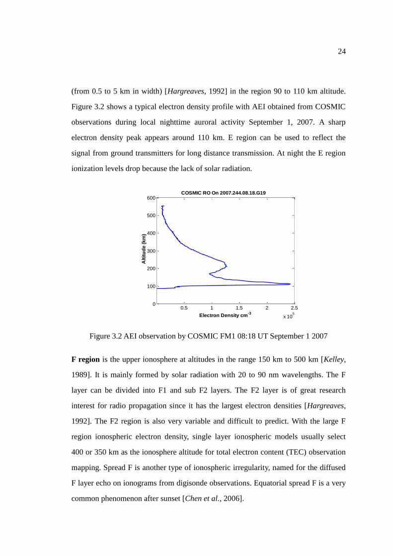
24
(from 0.5 to 5 km in width) [Hargreaves, 1992] in the region 90 to 110 km altitude.
Figure 3.2 shows a typical electron density profile with AEI obtained from COSMIC
observations during local nighttime auroral activity September 1, 2007. A sharp
electron density peak appears around 110 km. E region can be used to reflect the
signal from ground transmitters for long distance transmission. At night the E region
ionization levels drop because the lack of solar radiation.
0.5 1 1.5 2 2.5
x 105
0
100
200
300
400
500
600
Electron Density cm-3
Alt
itu
de
(k
m)
COSMIC RO On 2007.244.08.18.G19
Figure 3.2 AEI observation by COSMIC FM1 08:18 UT September 1 2007
F region is the upper ionosphere at altitudes in the range 150 km to 500 km [Kelley,
1989]. It is mainly formed by solar radiation with 20 to 90 nm wavelengths. The F
layer can be divided into F1 and sub F2 layers. The F2 layer is of great research
interest for radio propagation since it has the largest electron densities [Hargreaves,
1992]. The F2 region is also very variable and difficult to predict. With the large F
region ionospheric electron density, single layer ionospheric models usually select
400 or 350 km as the ionosphere altitude for total electron content (TEC) observation
mapping. Spread F is another type of ionospheric irregularity, named for the diffused
F layer echo on ionograms from digisonde observations. Equatorial spread F is a very
common phenomenon after sunset [Chen et al., 2006].
25
3.2 HIGH LATITUDE IONOSPHERE
3.2.1 MAGNETIC FIELD
The Earth’s magnetic field is close to a magnetic dipole. The earth’s magnetosphere
(which deviates from a symmetric dipole configuration) is produced by the electrical
charges’ (plasma) motion in near-Earth regions [Giraud and Petit, 1978]. The
magnetosphere acts to couple energy from the solar wind to the earth’s atmosphere
[Lyou, 2000]. Figure 3.3 shows behavior of the earth’s magnetic field under the effect
of solar wind [UCLA, 2009]. The solar wind carries the interplanetary magnetic field
(IMF) from the Sun outwards and has a strong influence on the earth’s atmosphere.
With the protection of the earth’s magnetosphere solar wind plasma cannot penetrate
the earth’s atmosphere directly. In Figure 3.3 the solar wind is deflected by the bow
shock of the earth on the dayside.
The dipolar terrestrial magnetic field is compressed by the high speed solar wind on
the dayside and stretched on the opposite nightside. The high energy particles are
accelerated by transferring the energy of solar wind into heating [Lyou, 2000]. The
Earth’s magnetic field is subject to irregular short-term fluctuation plus the ordinary
quasi-diurnal change due to large-scale electric current systems. The global Kp index
is used to measure the magnitude of magnetic perturbations at high latitudes [Giraud
and Petit, 1978]. The Kp index can characterize planetary magnetic (and ionospheric)
activities. Details of the Kp information can be found in Giraud and Petit [1978].

26
Figure 3.3 Earth’s magnetic field distorted under effects of solar wind [after
UCLA, 2009]
3.2.2 HIGH LATITUDE IONOSPHERIC IRREGULARITIES
Figure 3.4 shows the distribution of several types of ionospheric irregularities in the
high-latitude ionosphere. The plasmasphere is a region where the ions and electrons
are trapped by the earth’s magnetic field. Usually it extends up to 60 deg N
geomagnetic latitude in the night hemisphere. The poleward boundary is called the
plasmapause [Aarons, 1982]. A trough (localized low electron density region) exists at
geomagnetic latitude between 60 deg N to 65 deg N nightside. The plasmapause and
trough are located equatorward of the auroral oval and polar cap.

27
Figure 3.4 High latitude irregularities at auroral midnight [after Aarons, 1982]
3.2.2.1 AURORAL OVAL
The auroral oval is a region of closed magnetic field lines, which is characterized by
high conductivity, auroral electroject currents and precipitating electrons. Under
active conditions, energy from the solar wind is released into the auroral ionosphere
and precipitating electrons collide with neutral atmospheric constituents at
approximately 110 km altitude, resulting in visible aurora and variable total electron
content (TEC). The magnetosphere shields the Earth’s magnetic field from the solar
wind and highly energetic particles do not enter the ionosphere directly. The particles
will precipitate into the auroral oval along the magnetic field lines. The precipitation
occurs via field-aligned currents (Figure 3.5) and into the ionospheric electroject
region which is colocated with the auroral oval. Large-scale generation of
field-aligned currents is introduced by the precipitation plasma flows [Bates et al.,
1973]. Electrons with energies of 1 to 10 keV enter the atmosphere along the closed
magnetic field lines (mapping into the near-Earth magnetotail.)

28
Figure 3.5 Auroral substorm current wedge; the current closes westward through the
ionosphere at around 110 km [after Skone, et al., 2009]
Visible and ultraviolet radiation is emitted through collision of energetic electrons and
neutral atmospheric constituents, which is part of the phenomenon known as an
auroral substorm. Substorms are characterized by a wedge of electric current by
electrons coming from the near-Earth magnetotail (Figure 3.5) [Skone et al., 2009].
The localized ionospheric closure current can be observed by ground-based
magnetometers with perturbations in the H (north-south) component.
The enhancement of electron density at altitudes near 110 km, in the range 65-75 N
geomagnetic latitude after local midnight, is associated with auroral substorm activity.
Auroral precipitation creates irregularities in the E region - Auroral E-ionization
[Skone, 1998]. Small-scale instabilities corresponding to localized current structures
in the auroral ionosphere exist during geomagnetically disturbed periods [Hunsucker
et al., 1995]. Ionospheric electron density structures and irregularities exist with
horizontal scale sizes in the range 20 to 400 km [Baron, 1974]. Decorrelation of TEC
and GPS ionospheric range delays can occur over short distances (tens of kilometers).
AEI can have magnitudes comparable to the F region maximum with electron
densities in the range 2 - 20 ×1011
el/m3
[Baron, 1974].

29
3.2.2.2 POLAR CAP
The polar cap is at geomagnetic latitudes poleward of the auroral oval; this region
contains magnetic field lines open directly to the solar wind [Hunsucker and
Hargreaves, 2003]. The plasma can enter the ionosphere and becomes the source of
patches forming F region irregularities in the polar cap region [Rodger and Graham,
1996]. Polar cap irregularities do not exhibit as strong local time dependence as those
in the auroral oval [Aarons, 1982].
3.2.3 IONOSPHERIC PHENOMENA
Ionospheric phenomena and solar activities are highly related. The Sun emits
electromagnetic radiation over a wide spectral range which becomes the major energy
source of ionization of the ionosphere [Hargreaves, 1992]. Ionospheric phenomena
are caused by interaction of the solar wind and magnetosphere. Phenomena include
ionospheric storms, magnetic storms, auroral substorms, and traveling ionospheric
disturbances. Some relevant processes are described here.
Auroral Substorm is usually associated with auroral disturbances. It includes three
phases: growth phase, expansive and recovery phase. In the initial growth phase,
auroral oval boundaries expand equatorward. Ionospheric conductivity increases and
causes enhanced auroral electrojets and field-aligned currents. The growth phase is
characterized by a period of southward interplanetary magnetic field (IMF) and lasts
for several hours. Aurora occurs during the expansive phase when energetic particles
are accelerated from near-earth nightside regions down into the atmosphere. In this
phase intense aurora can be observed as the energetic particles precipitate (collide

30
with neutral atmospheric constituents and emit light). Large variations of electron
density will occur in both spatial and temporal domains during the expansive phase
and auroral E-ionization (AEI) can be observed in the E layer. Multiple expansions
can occur over several hours. During the recovery phase the ionosphere will return to
quiet conditions [Davies, 1990; Skone, 1998; Skone, 2007]. It should be noted that in
this thesis “storm” usually refers to magnetospheric/auroral substorm for simplicity.
The Kp and DST space weather indices can be used to measure the intensity of a local
midnight substorm.
Magnetic storm is a global event characterized by disturbances of the Earth’s
magnetic field. It includes three phases: initial phase, main phase and recovery phase.
These phases are identified in observations from low latitude magnetometers -
reflecting changes in the large-scale near-earth ring current [Skone, 2007].
Ionosphere storm is characterized by features of F region irregularities in electron
density [Skone, 1998]. Relations have been observed between ionospheric storms and
auroral substorms. But the two phenomena are not necessarily related. The ionosphere
storm can last for several days with severe effects on radiofrequency signals [Davies,
1990]. This event usually happens at mid-latitudes with associated variations
(negative and positive phases) in total electron content.
Another phenomenon arising from magnetic storms, with strong mid- and
high-latitude ionosphere electron density irregularities, is called storm enhanced
density (SED). This effect usually occurs during severe magnetic storm periods with
the feature of large TEC gradients at mid-latitudes. It is characterized by a plume of
total electron content extending mid- to high-latitude [Skone et al., 2005]. An example
of storm enhanced density on March 31, 2001 is shown in Figure 3.6. The plume with

31
large TEC values extends through high latitudes of Canada. For SED events, the large
TEC gradients can cause severe degradation of DGPS positioning accuracies. The
narrow enhanced TEC plume (for example the region between 40°N and 60°N
latitude) is also difficult to capture by sparse reference networks - such as for the
Wide Area Augmentation System (WAAS) [Skone, 2007].
Figure 3.6 Storm enhanced density on March 31, 2001 [after Skone et al., 2005]
3.3 IONOSPHERIC IMPACT ON GPS/GNSS SIGNALS
The ionosphere is an important error source for global navigation satellite systems.
The ionosphere has more variability in error than the troposphere, which makes it
difficult to model. For the ionosphere, the range error frequently changes at least one
order of magnitude diurnally, in addition to variable activity that can greatly affect the
ionospheric total electron content. The major ionospheric effects on GNSS signals are
group delay, carrier phase advance, Doppler shift, Faraday rotation, refraction or
bending of the signal, distortion of pulse waveforms, and scintillation effects
[Parkinson and Spilker, 1996].
32
3.3.1 FIRST ORDER EFFECT
Radio-waves propagating through the ionosphere will experience effects dependent
on the ionospheric electron content. The ionosphere is a dispersive medium which has
slightly different effects on GPS L1 and L2 signals. A GPS receiver can measure two
types of observables: code and carrier phase. The pseudorange and carrier phase
measurements are formed under the assumption that GPS signals travel at the speed of
light in a vacuum. However this assumption is not accurate in the ionosphere. It is the
same as incorrectly considering the phase and group indices of refraction pn and
gn
of the propagation medium to be equal to 1.
The phase range and pseudorange can be calculated as:
0 0
0path path path path
ct= dN= dN= d =
p p p
cdt
n n n
(3.1)
path path
= dt= dtg
g
cPR v
n (3.2)
where gv is the group velocity, c is the speed of light in vacuum, and 0 are
true wavelength and vacuum wavelength respectively. The term dN is the cycles of
carrier phase and dt is the travel time. Symbols and PR are carrier phase
range and pseudorange measurements in units of length.
In reality, the assumption of 1g pn n is not correct for ionospheric (or
tropospheric) signal propagation. For the ionosphere, pn and
gn can be expressed
as
33
22
2
0
22 22
21 1
1 1 1 40.32 2 2
p
p
Ne
m Nn
ff
(3.3)
where N is the ionospheric electron density, e is the electron charge, m is the
electron mass, 0 is the permittivity of free space, and f is the signal frequency.
Equation (3.3) shows that the phase index of refraction pn only depends on electron
density in the ionosphere N . For group index of refraction gn a similar expression
is
2 3 21 40.3 80.6 1 40.3
p
g p
dn N N Nn n f f
df f f f (3.4)
The term 2
40.3N
f is the difference from a vacuum medium. This leads to the group
delay and phase advance effects on GPS signals. The phase velocity is larger than the
speed of light in a vacuum by the amount
2
22
p
p
cv
(with the assumption of
being much larger thanp for GPS applications, where is the signal frequency
and p is the ionospheric plasma frequency). The group velocity is less than the
speed of light in a vacuum by the amount
2
22
p
g
cv
. In equations (3.3) and (3.4)
the higher order terms of ionospheric effects have been neglected due to a simplified
representation of the refractive index. Only zeroth and first-order terms are considered.
For the real ionosphere, magnetic field bending effects and the higher order
ionospheric delay terms can all affect signal propagation - contributing as much as 1
percent of the ionospheric range error [Brunner and Gu, 1991; Skone and Cannon,
1999]. Despite this, equations (3.3) and (3.4) can still be used to derive ionospheric
corrections for elimination of the first-order ionospheric effects using dual frequency

34
GPS receivers.
3.3.1.1 TEC MEASUREMENT
From another perspective, the existence of ionospheric delays for GPS signals can be
exploited to measure the electron content along a satellite-receiver line-of-sight. The
term 2
40.3N
f contributes to the ionospheric range error. After integrating, the range
delay can be derived as
2 2
40.3 40.3
path
Nds TECf f
(3.5)
The TEC is the total electron content along 1 m2 column along satellite-receiver
line-of-sight. Sometimes for modeling simplicity the ionosphere is assumed to consist
of a single very thin layer at 350 km, or 400 km, altitude.
Figure 3.7 Slant TEC is illustrated along a single satellite-receiver line-of-sight
[after Skone and Cannon, 1999]
35
Since GPS has multiple frequencies and the ionosphere is a dispersive medium, the
TEC can be calculated by differencing range measurements on L1 and L2.
1 2
2 2
1 2
1 1
1 140.3TEC PR PR
f f
(3.6)
For ionosphere modeling usually the slant TEC in Figure 3.7 and equation 3.6 should
be mapped to vertical TEC through multiplication by a mapping factor [details in
Schaer, 1999]. There are two kinds of TEC measurements based on code or phase
observations. Code-derived TEC is an absolute quantity derived with less precision
than for phase measurements. Phase-derived TEC is a relative quantity (containing
some biases). However, it has negligible noise and high precision. Dual frequency
GPS receivers use the relative TEC to smooth the rough but absolute
pseudorange-derived TEC to estimate first-order ionospheric range error corrections.
This process is done automatically and is transparent to the user [Skone, 1998; Schaer,
1999].
3.3.2 SCINTILLATION EFFECTS
One primary focus of this research is ionospheric scintillations. Such effects have an
impact on GNSS and satellite communications.
3.3.2.1 SCINTILLATION THEORY
Ionosphere scintillation is the rapid variation of signal amplitude or phase as the
signal passes through ionospheric electron density irregularities [Knight, 2000].

36
Scintillation appears principally in the trans-ionospheric signals, which is caused by
the relative phase shifts in the propagating wavefront and by subsequent diffraction
[Hunsucker and Hargreaves, 2003]. This is illustrated in Figure 3.8.
Figure 3.8 GPS signal propagating through the ionospheric electron density
irregularities [Skone et al, 2008].
From Huygen’s law, the wavefront is considered as a source of the secondary
wavelets to build up the wavefront at further points. In diffraction theory this law is
applied to determine how the amplitude and phase of a signal will change when
propagating through the irregularities. The requirement for amplitude scintillation is
that within the Fresnel zone distance there are several existing “small” irregularities
[Hunsucker and Hargreaves, 2003].
3.3.2.2 GLOBAL MORPHOLOGY OF IONOSPHERIC SCINTILLATIONS
Figure 3.9 shows the global distribution of ionospheric scintillations. Occurrence of
scintillation varies widely with the signal frequency, magnetic activities or solar
activities, local time, season, and latitude and longitude [Aarons, 1982]. There is an
obvious nighttime maximum globally. For the nighttime high-latitude region auroral
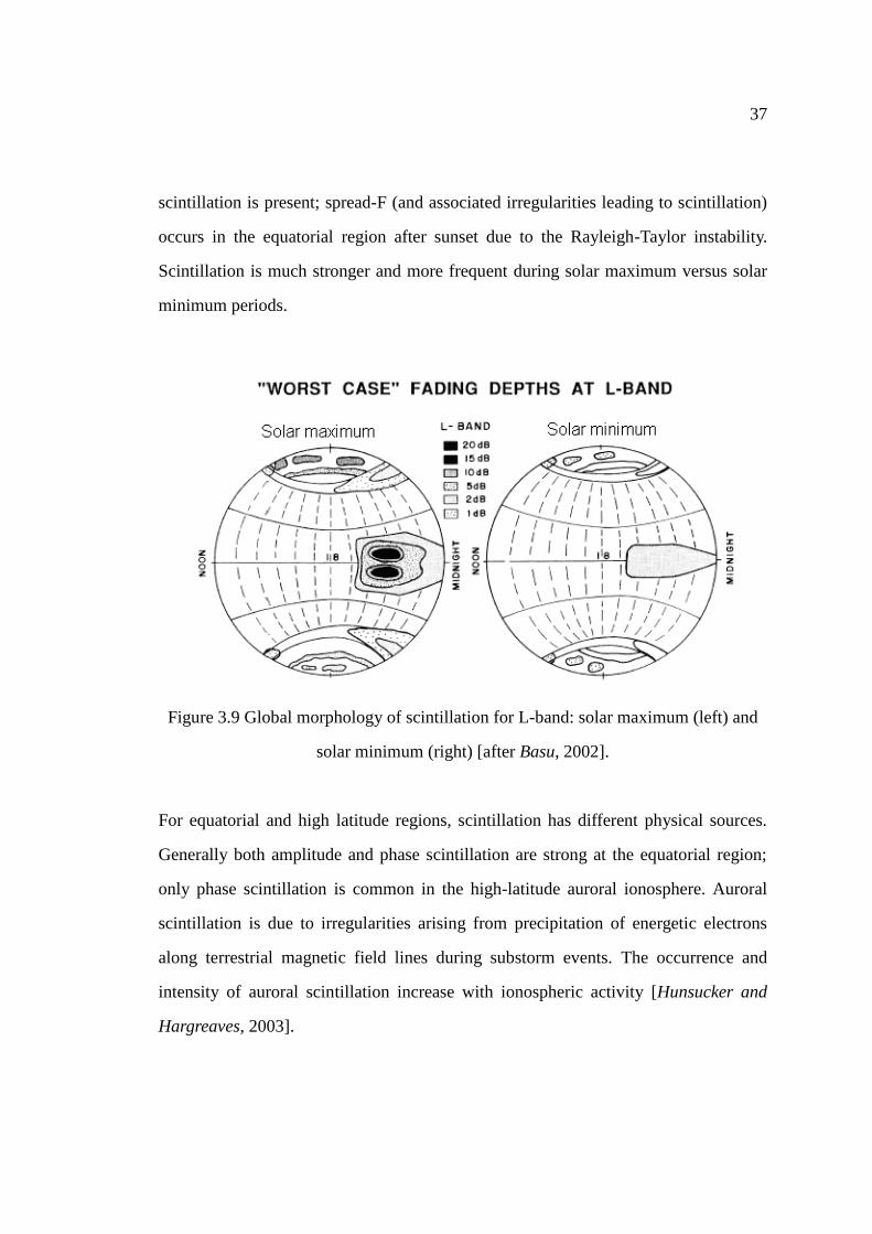
37
scintillation is present; spread-F (and associated irregularities leading to scintillation)
occurs in the equatorial region after sunset due to the Rayleigh-Taylor instability.
Scintillation is much stronger and more frequent during solar maximum versus solar
minimum periods.
Figure 3.9 Global morphology of scintillation for L-band: solar maximum (left) and
solar minimum (right) [after Basu, 2002].
For equatorial and high latitude regions, scintillation has different physical sources.
Generally both amplitude and phase scintillation are strong at the equatorial region;
only phase scintillation is common in the high-latitude auroral ionosphere. Auroral
scintillation is due to irregularities arising from precipitation of energetic electrons
along terrestrial magnetic field lines during substorm events. The occurrence and
intensity of auroral scintillation increase with ionospheric activity [Hunsucker and
Hargreaves, 2003].
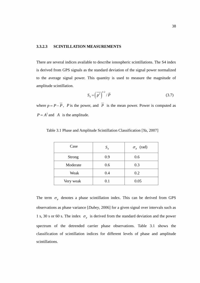
38
3.3.2.3 SCINTILLATION MEASUREMENTS
There are several indices available to describe ionospheric scintillations. The S4 index
is derived from GPS signals as the standard deviation of the signal power normalized
to the average signal power. This quantity is used to measure the magnitude of
amplitude scintillation.
1/ 2
2
4 /S p P (3.7)
where p P P , P is the power, and P is the mean power. Power is computed as
2P A and A is the amplitude.
Table 3.1 Phase and Amplitude Scintillation Classification [Yu, 2007]
Case 4S (rad)
Strong 0.9 0.6
Moderate 0.6 0.3
Weak 0.4 0.2
Very weak 0.1 0.05
The term denotes a phase scintillation index. This can be derived from GPS
observations as phase variance [Dubey, 2006] for a given signal over intervals such as
1 s, 30 s or 60 s. The index is derived from the standard deviation and the power
spectrum of the detrended carrier phase observations. Table 3.1 shows the
classification of scintillation indices for different levels of phase and amplitude
scintillations.

39
GPS receivers experience degraded performance under scintillation conditions [Leick,
1995]. Amplitude fades may cause the signal to noise ratio (SNR) to drop below the
receiver tracking threshold, resulting in a loss of code or phase lock. Strong phase
scintillation may cause high phase dynamics (large frequency Doppler shifts) in GPS
carrier signals; if such dynamics exceed the receiver’s PLL (phase lock loop)
bandwidth a loss of phase lock will occur. For semicodeless or codeless tracking
technologies the signal will have an average loss of 14 to 17 dB and 27 to 30 dB
[Leick, 1995]. In such cases the L2P(Y) PLL employs a narrow bandwidth of 1 Hz
(compared with 15 Hz for L1) in order to eliminate excess noise. The result is that
L2P(Y) is more susceptible to phase scintillation effects. Scintillation effects have
been observed in many GPS observations. Some examples are shown in the next
section.
3.3.2.4 PHASE CYCLE SLIPS
GPS phase cycle slips are loss of signal lock in the GPS receiver tracking loop. A
cycle slip is observed as a discontinuity in the phase integer ambiguity. Cycle slips
can occur under ionospheric scintillation conditions when high phase dynamics
(exceeding receiver tracking loop bandwidths) arise from ionospheric irregularities.
Figure 3.10 shows scintillation observations at Natal, Brazil for a solar maximum
period [Aarons, 1993] and Figure 3.11 shows cycle slip occurrence at IGS BRAZ
station in 2001. The cycle slip is calculated from TECMODEL software [Skone, 2006].
Good correlation can be found between the two plots, which illustrate the strong
effects of ionospheric scintillation on GPS receivers. For the equatorial region,
seasonal variations in scintillation are also found to be a function of longitude
[Beaujardiere et al., 2004].

40
Figure 3.10 Intensity of scintillation data at Brazil [after Aarons, 1993]
0 40 80 120 160 200 240 280 320 3600
1
2
3
4
Day of Year
Co
rru
pt O
bse
rva
tion
s %
BRAZ 2001
Figure 3.11 Daily occurrence of cycle slip for BRAZ station in 2001
Another example of cycle slip occurrence for a high latitude International GNSS
Service (IGS) GPS station Yellowknife is shown in Figure 3.12. October 29 and 30
2003 are two days with severe geomagnetic storms within the whole Canadian region.
The global Kp index for this period is shown in Figure 3.13. The average Kp value is
higher than eight for the two disturbed days (Kp maximum possible value is nine).
Accordingly the data for Yellowknife shows obvious high occurrence of GPS signal
phase cycle slips for the two days time period. Both of the two examples in Figure
3.11 and Figure 3.12 show the occurrence correlation between ionospheric
irregularities (present during the inferred high levels of ionospheric activity) and of
corrupt observations at local IGS stations.

41
Figure 3.12 Daily occurrence of cycle slip for Yellowknife from October 14
to November 13 2003
0
1
2
3
4
5
6
7
8
9
Oct 30 Oct 29 Oct 30 Oct31
K I
ndex
Oct 28~Oct 31 2003
Red : Kp>=8
Figure 3.13 Kp index for October 28 to 31 2003
3.3.2.5 GPS POSITIONING ERROR
Scintillation effects can add perturbations and cause additional noise on GPS signals,
with an impact on positioning accuracy. Correlation between scintillation intensity
and position error have been studied by Dubey et al. [2005].

42
Figure 3.14 (a) Scintillation intensity (represented by size of circles) from 1200 to
1600 UT on March 19, 2001; (b) Latitudinal and longitudinal error of GPS position in
meters [after Dubey et al., 2006]. The blue line is latitudinal error and the green line is
longitudinal error.

43
Figure 3.14 (a) shows the S4 plots for a GPS ionospheric scintillation monitor in the
low latitude region (Chiang Rai, Thailand) 1200 to 1600 UT 19 March 2001. Figure
3.14 (b) shows the latitudinal and longitudinal variations of GPS positions for a fixed
location nearby (19.6 ° N, 99.5° E). An intense scintillation period is observed
between 1400 and 1500 UT (2100 to 2200 LT) with a maximum S4 index. The
latitudinal error reaches 22 m and longitudinal error reaches 14 m [Dubey et al., 2006].
This event is a typical case of equatorial irregularities causing scintillation after sunset
during a solar maximum period.
3.3.2.6 FLUCTUATION OF RADIO OCCULTATION SIGNAL SNR
Figure 3.15 shows the SNR for GPS C/A code for a single CHAMP RO occultation
event February 25, 2002. This is an event in the nighttime equatorial region. In the
equatorial region after sunset the spread-F scintillation can be severe.
Figure 3.15 SNR plot for one radio occultation event for CHAMP on February 22,
2002 [after Straus et al., 2003]

44
In Figure 3.15 the C/A SNR fluctuates a large amount in the F layer altitudes
(300-500 km); this is the result of irregularities in the F region ionosphere. Another
scintillation event is observed in the high-latitude auroral region during a disturbed
period. Figure 3.16 is the detrended RO signal SNR on July 10, 2005. The
low-frequency trend of the profile is removed from the profile. High-frequency
fluctuations are observed near 110 km altitude for both L1 and L2 signals; this
corresponds to the AEI feature typical in the auroral region during substorms.
-40 -20 0 20 400
100
200
300
400
C/A SNR (V/V)
Altitude (
km
)
2005 Jul 10
-40 -20 0 20 400
100
200
300
400
L2 SNR (V/V)
Figure 3.16 Detrended SNR plot for high-latitude radio occultation
45
CHAPTER 4
RADIO OCCULTATION TECHNIQUE
In this chapter general theory of radio occultation will be covered along with the Abel
inversion retrieval method. The CHAMP and COSMIC missions are also introduced.
4.1 OVERVIEW OF RADIO OCCULTATION TECHNIQUE
Radio occultation missions such as CHAMP and COSMIC are used to sound the
earth’s neutral atmosphere and ionosphere via a radio link between a GPS navigation
satellite and GPS receivers equipped on low Earth orbiter (LEO) satellites [Lee et.al.,
2001; Gorbunov, 1996]. Initially, radio occultation satellites were launched to sound
other planets’ atmospheres and surfaces in our solar system. The United States GPS
meteorology (GPS/MET) experiment was the first mission to apply the radio
occultation technique to the Earth successfully using GPS signals. Figure 4.1 is a
diagram illustrating the RO technique. The direct radio link between the GPS and
LEO satellite is occulted by the Earth’s limb; as the electromagnetic radiation passes
through the atmosphere it is refracted. The link between the two satellites can be
maintained due to the refraction of signal. Signals received by the GPS receiver
onboard the LEO includes propagation delays due to properties of the given
atmospheric layer.

46
Figure 4.1 Concept of radio occultation observations
The magnitude of the refraction depends on the nature of the atmosphere. The
bending of the signal is usually determined by the neutral components in the
atmosphere or ionospheric electron density. As the LEO-GPS line-of-sight is occulted
by the Earth’s limb with the setting (or sometimes rising) movement of the LEO
satellite, the GPS-LEO radio link successively scans the atmospheric layers at
different altitudes. Refractivity profiles of the atmosphere are retrieved from such
GPS-LEO signal observations by applying the Abel inversion; the fundamental
observation for this processing is the excess phase delay caused by the propagation
medium. As illustrated in Figure 4.1, for example, the earth’s atmosphere can be
assumed to consist of multiple layers; each layer is sounded by the RO signal
successively as the GPS-LEO line-of-sight moves downward. The refractivity
gradient of the first layer is later used to calculate the refractivity of the second layer,
and the first and the second sounding provide the refractivity information to calculate
the third layer’s refractivity. Therefore, layer by layer, the vertical refractivity profile
will be estimated as if peeling layers of an onion. The method of retrieving electron
density will be explained in detail in the next section. Effects of the atmosphere on
radio occultation signals are summarized by Hajj et al. [2002].
GPS 1
2 3
LEO
47
Atmospheric and ionospheric effects cause the change of signal and are measured to
reveal information about atmospheric properties for different layers. Investigations
have already proven that the accuracies of RO atmospheric retrieval parameters are
comparable, if not better, than other traditional sensing methods [Hajj et al., 2002].
Radio occultation techniques provide promising application in meteorology,
climatology and ionospheric physics.
LEO-GPS missions are able to obtain vertical profiles of refractivity, density, pressure,
temperature and water vapor pressure in the neutral atmosphere and electron density
in the ionosphere. Applications include climate change detection, numerical weather
predictions, gravity wave morphology studies, and ionospheric tomography. With
more missions being conducted (and proposed), radio occultation techniques are
expected to provide the advantage of all-weather, global coverage, high vertical
resolution and long-term stability.
4.2 CHAMP AND COSMIC MISSIONS
4.2.1 CHAMP
The German CHAMP (CHAllenging Minisatellite Payload) satellite was launched
from Plesetsk, Russia on July 15, 2000 by a COSMOS rocket. The primary purpose of
this mission is precise gravity studies, magnetic field measurement and
atmosphere/ionosphere sounding by radio occultation techniques [Jakowski et al.,
2002]. It carries the latest RO receiver from JPL (Jet Propulsion Laboratory, USA).
The GPS flight receiver (“BlackJack”) is specially designed for radio occultation

48
sounding purposes. The enhanced L2 signal noise introduced by GPS antispoofing is
reduced by the application of a high-gain GPS antenna to some extent, with higher
signal to noise ratio than normal receivers [Wickert et al., 2001]; this reduces the
impact of GPS antispoofing effects on CHAMP’s LEO receiver.
The CHAMP satellite orbit is almost circular and near-polar which is designed for
homogeneous and better global coverage to remotely sense the earth’s atmosphere
with an inclination angle of 87.2 and initial altitude of 454 km [Wickert et al., 2005].
The first CHAMP profiling experiment commenced operating on 11 February 2001
[Wickert et al., 2001] and CHAMP continues to operate. CHAMP data are available at
various levels and are publicly available at the CHAMP Information System and Data
Center (ISDC) at the GFZ website: http://op.gfz-potsdam.de/champ. CHAMP data can be
divided into three types: Atmosphere/Ionosphere, Orbit/Gravity, and
Magnetic/Electric Field. Various levels of data exist in all three categories. Table 4.1
provides the classification of Atmosphere/Ionosphere CHAMP data. In this catalog
the phase observations of L1 and L2 for the LEO onboard receiver and ground
receiver are available in Level 1. The excess phase delay product, which is used to
retrieve atmospheric parameters - such as electron density - is a Level 2 product.
The occultation table which provides a list of occultation events by date and time is in
Level 2. In Level 3 the final products such as parameters of neutral atmosphere,
electron density, and TEC along the GPS-LEO line of-sight are available. An average
delay of 3 to 4 hours exists between measurements onboard CHAMP (Level 1) and
the provision of the analysis data (excess phase of Level 2) [Wickert et al., 2005].

49
Table 4.1 Classification of CHAMP Data under Atmosphere/Ionosphere Category
[ISDC, 2009]
Product type Description Format
Level 1
CH-A1-1-GPS-01S High rate GPS ground tracking data, 1 Hz RINEX
2.20
CH-A1-1-HR High rate CHAMP GPS-SST, 50 Hz, RINEX
2.10
CH-A1-1-MR Medium rate CHAMP GPS-SST, 1Hz RINEX
2.10
Level 2 CH-A1-2-PD Atmospheric excess path delay ASC II
CH-A1-2-TAB Occultation tables ASC II
Level 3
CH-A1-3-ATM Atmospheric parameters ASC II
CH-A1-3-IVP Vertical electron density profiles ASC II
CH-A1-3-TCR Occultation link related TEC data ASC II
For ionosphere altitudes the resolution is from 0.5 to 3 km for 1 Hz data and
approximately 30 m for 50 Hz data; this depends on the vertical RO ray path velocity.
Moreover the altitude coverage is different between 50 Hz and 1 Hz products. The 50
Hz data usually starts around 130 km altitude, and is mainly used to measure the
troposphere parameters and detect the sporadic E layer, while 1 Hz data starts around
400 km altitude and covers the ionospheric F1 region. There are approximately 200 to
250 CHAMP radio occultation events per day with locations distributed across the
earth’s surface depending on the satellite’s ephemeris [Wickert et al., 2001]. The
CHAMP orbit changes the local time coverage by approximately 5.6 min per day for
the equatorial region. It covers the 24 hour cycle for 130 days. The pattern repeat
period could be shorter since the broad antenna field of view for CHAMP’s RO
receiver can possibly allow occultation from GPS satellites within ± 1 hour [Wu,
2006].
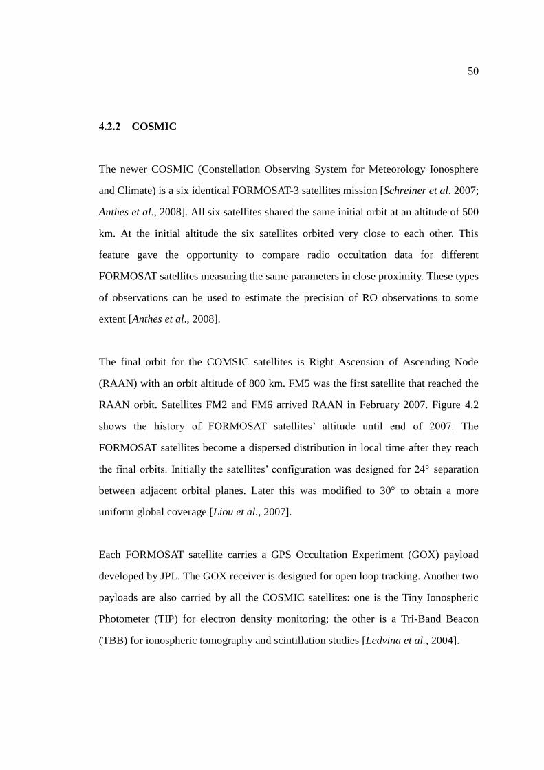
50
4.2.2 COSMIC
The newer COSMIC (Constellation Observing System for Meteorology Ionosphere
and Climate) is a six identical FORMOSAT-3 satellites mission [Schreiner et al. 2007;
Anthes et al., 2008]. All six satellites shared the same initial orbit at an altitude of 500
km. At the initial altitude the six satellites orbited very close to each other. This
feature gave the opportunity to compare radio occultation data for different
FORMOSAT satellites measuring the same parameters in close proximity. These types
of observations can be used to estimate the precision of RO observations to some
extent [Anthes et al., 2008].
The final orbit for the COMSIC satellites is Right Ascension of Ascending Node
(RAAN) with an orbit altitude of 800 km. FM5 was the first satellite that reached the
RAAN orbit. Satellites FM2 and FM6 arrived RAAN in February 2007. Figure 4.2
shows the history of FORMOSAT satellites’ altitude until end of 2007. The
FORMOSAT satellites become a dispersed distribution in local time after they reach
the final orbits. Initially the satellites’ configuration was designed for 24 separation
between adjacent orbital planes. Later this was modified to 30 to obtain a more
uniform global coverage [Liou et al., 2007].
Each FORMOSAT satellite carries a GPS Occultation Experiment (GOX) payload
developed by JPL. The GOX receiver is designed for open loop tracking. Another two
payloads are also carried by all the COSMIC satellites: one is the Tiny Ionospheric
Photometer (TIP) for electron density monitoring; the other is a Tri-Band Beacon
(TBB) for ionospheric tomography and scintillation studies [Ledvina et al., 2004].
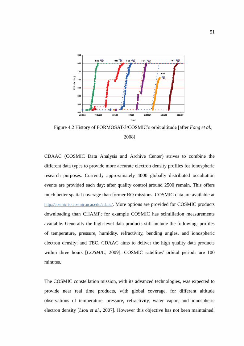
51
Figure 4.2 History of FORMOSAT-3/COSMIC’s orbit altitude [after Fong et al.,
2008]
CDAAC (COSMIC Data Analysis and Archive Center) strives to combine the
different data types to provide more accurate electron density profiles for ionospheric
research purposes. Currently approximately 4000 globally distributed occultation
events are provided each day; after quality control around 2500 remain. This offers
much better spatial coverage than former RO missions. COSMIC data are available at
http://cosmic-io.cosmic.ucar.edu/cdaac/. More options are provided for COSMIC products
downloading than CHAMP; for example COSMIC has scintillation measurements
available. Generally the high-level data products still include the following: profiles
of temperature, pressure, humidity, refractivity, bending angles, and ionospheric
electron density; and TEC. CDAAC aims to deliver the high quality data products
within three hours [COSMIC, 2009]. COSMIC satellites’ orbital periods are 100
minutes.
The COSMIC constellation mission, with its advanced technologies, was expected to
provide near real time products, with global coverage, for different altitude
observations of temperature, pressure, refractivity, water vapor, and ionospheric
electron density [Liou et al., 2007]. However this objective has not been maintained.

52
Figure 4.3 shows the COSMIC RO observation coverage for 100 min centered at
14:00 UT March 4, 2007. Different colors represent observations from different FM
satellites. It is observed that not all the longitude sectors are covered during the
specified 100 min.
Figure 4.3 Transionospheric radio links between COSMIC satellites and GPS for 100
min, centered on 14:00 UT March 4, 2007. [after Anthes et al., 2008]
A follow-up mission COSMIC II has been proposed. Improvements include
processing of Galileo/GLONASS satellite signals. The latency of data processing is
also expected to be greatly reduced. And a more improved tracking capability and
antenna gain will allow lowest altitude moist troposphere sensing. Finally COSMIC II
will also provide 12 additional LEO satellites in space. The future COSMIC II will be
more challenging and powerful for ionospheric research and space weather
forecasting.
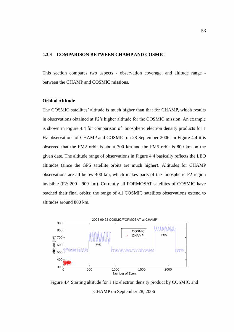
53
4.2.3 COMPARISON BETWEEN CHAMP AND COSMIC
This section compares two aspects - observation coverage, and altitude range -
between the CHAMP and COSMIC missions.
Orbital Altitude
The COSMIC satellites’ altitude is much higher than that for CHAMP, which results
in observations obtained at F2’s higher altitude for the COSMIC mission. An example
is shown in Figure 4.4 for comparison of ionospheric electron density products for 1
Hz observations of CHAMP and COSMIC on 28 September 2006. In Figure 4.4 it is
observed that the FM2 orbit is about 700 km and the FM5 orbit is 800 km on the
given date. The altitude range of observations in Figure 4.4 basically reflects the LEO
altitudes (since the GPS satellite orbits are much higher). Altitudes for CHAMP
observations are all below 400 km, which makes parts of the ionospheric F2 region
invisible (F2: 200 - 900 km). Currently all FORMOSAT satellites of COSMIC have
reached their final orbits; the range of all COSMIC satellites observations extend to
altitudes around 800 km.
0 500 1000 1500 2000300
400
500
600
700
800
900
Number of Event
Altitu
de
(km
)
2006 09 28 COSMIC/FORMOSAT vs CHAMP
COSMIC
CHAMP
FM2
FM5
Figure 4.4 Starting altitude for 1 Hz electron density product by COSMIC and
CHAMP on September 28, 2006

54
Observation Coverage
From Figure 4.4 it can be observed that COSMIC has more records for electron
density product than CHAMP on a single day. This is due to the number of LEOs
available: COSMIC mission has a constellation of six satellites and CHAMP is a
one-satellite mission. Observation coverage for one day (September 28 2006) is
shown for COSMIC and CHAMP in Figures 4.5 and 4.6. There are 3937 events for
COSMIC and 814 for CHAMP before the quality control. In Figure 4.6 it is observed
that for one day the observations of CHAMP are sparse and cannot provide global
overage compared with COSMIC. There is a very distinct longitude selection for
CHAMP.
Figure 4.5 COSMIC observations coverage on September 28, 2006

55
Figure 4.6 CHAMP observations coverage on September 28, 2006
4.3 RADIO OCCULTATION DATA PROCESSED BY CDAAC
For RO missions (eg: COSMIC, CHAMP) there are generally two kinds of data rates
provided. One is 50 Hz for lower atmosphere (troposphere) observations and the other
is 1 Hz for ionosphere observations. Spatial resolution is directly dependent on data
rate. An example of a CHAMP RO event is shown in Figure 4.7. Usually 1 Hz data
can cover the major part of the ionosphere (e.g. F layer) with adequate spatial
resolution while the 50 Hz data with higher resolution can only provide observations
for lower E and D region. The lack of high rate observations for the ionosphere F
region arises from considerations of data management onboard the satellite.

56
CDAAC (COSMIC Data Analysis and Archival Center) has developed a GPS RO
data processing system for COSMIC. The retrieval methods are introduced with
reference to information provided on the CDAAC website [COSMIC, 2009].
0 0.5 1 1.5 2 2.5 30
50
100
150
200
250
300
350
400
20060930 raw observation
L1-L2
Alt
itu
de
(K
m)
1Hz
50 Hz
Figure 4.7 Altitude coverage of 1 Hz (blue) and 50 Hz (red) observations for one RO
event from CHAMP dataset
4.3.1 ALGORITHMS FOR RADIO OCCULTATION INVERSIONS IN THE
IONOSPHERE
For COSMIC, the inversion method for ionosphere radio occultation is based on an
assumption of local spherical symmetry. The assumption is that the electron density
within a few thousand kilometers radius around the tangent point of the ray path is
locally spherically symmetric. This assumption cannot always be valid since it ignores
the physical presence of horizontal density gradients. The retrieved electron density
profile may have errors in cases when ionospheric conditions differ greatly from
assumptions. In particular, for altitudes below the E region negative values can often

57
be found in the density profiles generated by CDAAC. Another issue of note is that
the vertical electron density profile is determined for different horizontal geographic
locations of the ray path bottom versus top; the horizontal distance bottom versus top
of the profile can be one hundred kilometers. The profile does not represent the
ionosphere for the same longitude and latitude at different altitudes.
Phase measurements of the RO signal are fundamental observations necessary to
derive the refractivity. The refractivity is then used to derive the electron density
profile in the ionosphere (or temperature and pressure profile in the neutral
atmosphere). Abel inversion is a common technique for processing RO data which is
sensitive to vertical structures. The GPS/MET mission was the first to perform the
application of Abel inversion to RO retrieval. Usually there are two types of retrieval
based on different kinds of observations. One is based on bending angle. The other is
based on slant total electron content (STEC) observations [Garcia-Fernandez, 2002;
Schreiner, 1999]. Only the second method is introduced here.
4.3.1.1 ABEL INVERSION
In physics or engineering it is common to have two functions such that one is the
integration of the other: ( ) ( ) ( , )b
af a g t K t dt . The function ( )f a is the integral
transform of the function ( )g t . As the integral transforms comprise a special subset of
the equations, the inverse transform can be found as follows: ( ) ( ) ( , )g t f a t da
.
One of the widely used integral transforms is the Fourier transform. Abel transform is
another one that has requirements for both of the functions. The Abel transform is
widely applied for atmospheric profile retrievals using radio occultation observations.

58
The general transform can be defined as follows:
0( ) ( ) ( , )f a g r K r a dr
(4.1)
where 2 2
2
( , )
0
rif r a
K r a r a
otherwise
or alternatively 2 2
2( ) ( )
a
rf a g r
r a
(4.2)
In many applications the function ( )f a is an abscissa function and ( )g r is a radial
function. The variables r and a represent a radius and an abscissa respectively. An
inverse Abel transform exists in the form
2 2
1 ( )( )
r
f ag r da
a r
(4.3)
For more description of Abel inversion one can refer to [Eshleman, 1973] and [Hinson
et al., 1998]. For GPS RO usually ( )g r is the electron density as a function of
altitude and ( )f a is the TEC measurement along the GPS-LEO ray. The Abel
inversion is applied to electron density retrieval and will be discussed in the next
section.
4.3.1.2 INVERSION USING SLANT TEC MEASUREMENTS
Inversions based on slant TEC measurements should assume that the LEO-GPS ray
bending angle is very small. For the ionospheric F region altitude this assumption is
valid. The inversion based on slant TEC (STEC) is an onion-peeling method as

59
illustrated in Figure 4.1. Details of this method can be found in Garcia-Fernandez
[2002] and Schreiner et al. [1999]. For electron density retrieval by CDAAC this
method is used instead of using inversions from bending angle.
Figure 4.8 Illustration of occultation geometry with straight line GPS-LEO ray [after
Garcia-Fernandez, 2002]
Total electron content (TEC) along the GPS-LEO ray can be expressed as follows.
2 2
6EC ( 1)
40.3 10 40.3
f f ST Ndl n dl
(4.1)
where N is electron density, n is the ionospheric index of refractivity and S is the
excess phase product (which is obtained directly from COSMIC data archives). TEC
can be calculated from either L1 or L2 excess phase observations or from a linear
combination of both:
2 2 2
1 1 2 2 2 21 2
2 2
2 1
1 1TEC
1 140.3 40.3 40.3 40.3
f S f S f SS S
f f
(4.2)
TEC computation from a single frequency observation contains effects of orbital
motion and drifts of GPS transmitter and receiver clocks; these must be estimated
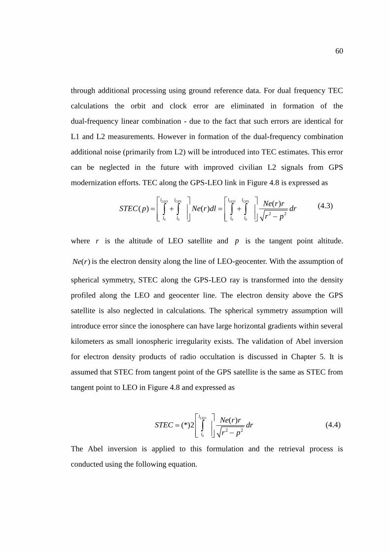
60
through additional processing using ground reference data. For dual frequency TEC
calculations the orbit and clock error are eliminated in formation of the
dual-frequency linear combination - due to the fact that such errors are identical for
L1 and L2 measurements. However in formation of the dual-frequency combination
additional noise (primarily from L2) will be introduced into TEC estimates. This error
can be neglected in the future with improved civilian L2 signals from GPS
modernization efforts. TEC along the GPS-LEO link in Figure 4.8 is expressed as
(4.3)
where r is the altitude of LEO satellite and p is the tangent point altitude.
( )Ne r is the electron density along the line of LEO-geocenter. With the assumption of
spherical symmetry, STEC along the GPS-LEO ray is transformed into the density
profiled along the LEO and geocenter line. The electron density above the GPS
satellite is also neglected in calculations. The spherical symmetry assumption will
introduce error since the ionosphere can have large horizontal gradients within several
kilometers as small ionospheric irregularity exists. The validation of Abel inversion
for electron density products of radio occultation is discussed in Chapter 5. It is
assumed that STEC from tangent point of the GPS satellite is the same as STEC from
tangent point to LEO in Figure 4.8 and expressed as
0
2 2
( )(*)2
LEOl
l
Ne r rSTEC dr
r p
(4.4)
The Abel inversion is applied to this formulation and the retrieval process is
conducted using the following equation.
0 0 0 0
2 2
( )( ) ( )
LEO GPS LEO GPSl l l l
l l l l
Ne r rSTEC p Ne r dl dr
r p
61
2 2
1 ( ) /( )
LEOr
e
r
dSTEC p dpN r dp
p r
(4.5)
In processing conducted by CDAAC to retrieve the electron density, the measured and
calibrated TEC is inverted to an electron density profile using the onion peeling
method:
,
11
( )3( ) ( )
4 2 ( )
n ii
e i k i e i k
ki i i
TEC pN p c N p
p p p
(4.6)
where the coefficients, ,k ic are derived in Syndergaard et al. [2004], eN is the
electron density, and p is the impact parameter. Index i stands for different layers in
the ionosphere. Usually the electron density obtained for higher altitude layers will be
used to retrieve electron density for lower altitude layers during a RO event. For more
about the ionospheric electron density retrieval method one can refer to the
documentation on CDAAC website [COSMIC, 2009].
62
CHAPTER 5
VALIDATION OF RADIO OCCULTATION OBSERVATIONS BY GROUND
OBSERVATIONS
5.1 GROUND OBSERVATIONS
In addition to radio occultation observations from COSMIC and CHAMP, several
complementary high-latitude datasets are used in the studies presented here. This
chapter contains a brief introduction to the ground datasets. Some datasets are used
for validation; other datasets are used in later chapters to identify the presence of
ionospheric disturbances.
5.1.1 SCINTILLATION OBSERVATIONS
Since 2003 the University of Calgary has operated several GPS scintillation receivers
in Canada. Scintillation is recorded by three GPS receivers as part of CANGIM
(CANadian GPS Network for Ionosphere Monitoring). The receivers are NovAtel
Euro4 receivers capable of deriving phase and amplitude scintillation information.
Figure 5.1 shows their locations. The three stations are almost aligned along the same
meridian at different latitudes spanning the sub-auroral, auroral and polar cap regions
(depending on level of ionospheric activity). Yellowknife is a high latitude site where
aurora is commonly observed. In this thesis nightside auroral scintillation conditions
are identified from the extensive CANGIM GPS dataset.

63
Figure 5.1 Geodetic locations of three scintillation GPS receivers: Calgary, Athabasca,
Yellowknife [Skone et al., 2008]
5.1.2 MAGNETOMETER OBSERVATIONS
The level of magnetic activity is recorded in magnetometer observations. Local
magnetometer observations are more related to local ionospheric disturbed conditions
than the global Kp geomagnetic index. There are two websites with relevant publicly
available magnetometer datasets. One is maintained by GSC (Geological Survey of
Canada): http://geomag.nrcan.gc.ca. The other is the CSSDP (Canadian Space Science
Data Portal): http://portal.cssdp.ca. GSC and CSSDP magnetometer sites are shown in
Figures 5.2 and 5.3 respectively. CARISMA (Canadian Array for Realtime
Investigations of Magnetic Activity) stations from CSSDP are shown. There are sites
along the same meridian (from TALO to PINA) in CARISMA; these are used to infer
the auroral oval boundaries.

64
-140 -130 -120 -110 -100 -90 -80 -70 -60 -50 -4030
40
50
60
70
80
90
BLC
BRD
CBB
EUA
FCC
GLN
IQA
MEA
OTT
PBQ
RES
STJVIC
YKC
SNK
Longitude (deg)
La
titu
de
(d
eg
)
Canadian Magnetic Observatories
Figure 5.2 Geodetic locations of GSC Observations
Figure 5.3 Geodetic locations of CARISMA magnetometers [CARISMA, 2009]
Another magnetometer array called GIMA (Geophysical Institute Magnetometer
Array) is also used to validate the disturbed ionospheric conditions. These sites are
close to the incoherent scatter radar PFISR in Alaska.
Magnetometers of GSC

65
5.1.3 INCOHERENT SCATTER RADAR
Incoherent Scatter Radar (ISR) data are used to validate the electron density profiles
from radio occultation. ISR data can be downloaded from the Madrigal database
maintained by Haystack Observatory. Madrigal is a database of ground-based
measurements and models of upper atmosphere and ionosphere [AMISR, 2009].
Locations of the world’s incoherent scatter radars are shown in Figure 5.4 [Haystack,
2009]. The AMISR at top left of the map is in Poker Flat ISR (PFISR) in Alaska.
Figure 5.4 Geodetic locations of ISR instruments [after Haystack, 2009]
All such ground-based instruments assist in the analysis of radio occultation
capabilities. In the following section RO measurements are validated by ISR and
ionosonde. For the purposes of this thesis only measurements for ionosphere (no
troposphere) are validated.

66
5.2 VALIDATION BY INCOHERENT SCATTER RADAR
5.2.1 PUBLISHED VALIDATION
Incoherent scatter radar can be used to validate radio occultation electron density
measurements - since it can provide the whole electron density profile. Lei et al.
[2007] compared electron densities from COSMIC RO observations with ISR. Data
from June 27 to July 1 and September 20-22 2006 at Millstone Hill and Jicamarca
were used.
Figure 5.5 Six comparisons of electron density profiles between COSMIC RO (solid
lines) and Millstone Hill ISR (circles). Error bars are standard deviations for the ISR
data over 1 hour [after Lei et al., 2007]
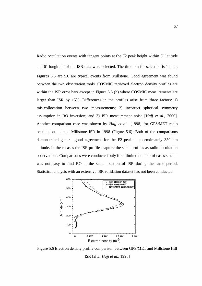
67
Radio occultation events with tangent points at the F2 peak height within 6° latitude
and 6° longitude of the ISR data were selected. The time bin for selection is 1 hour.
Figures 5.5 are 5.6 are typical events from Millstone. Good agreement was found
between the two observation tools. COSMIC retrieved electron density profiles are
within the ISR error bars except in Figure 5.5 (b) where COSMIC measurements are
larger than ISR by 15%. Differences in the profiles arise from three factors: 1)
mis-collocation between two measurements; 2) incorrect spherical symmetry
assumption in RO inversion; and 3) ISR measurement noise [Hajj et al., 2000].
Another comparison case was shown by Hajj et al., [1998] for GPS/MET radio
occultation and the Millstone ISR in 1998 (Figure 5.6). Both of the comparisons
demonstrated general good agreement for the F2 peak at approximately 350 km
altitude. In these cases the ISR profiles capture the same profiles as radio occultation
observations. Comparisons were conducted only for a limited number of cases since it
was not easy to find RO at the same location of ISR during the same period.
Statistical analysis with an extensive ISR validation dataset has not been conducted.
Figure 5.6 Electron density profile comparison between GPS/MET and Millstone Hill
ISR [after Hajj et al., 1998]
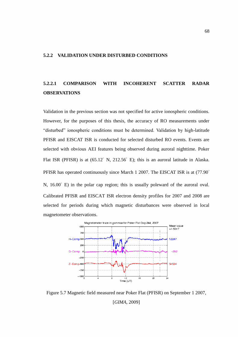
68
5.2.2 VALIDATION UNDER DISTURBED CONDITIONS
5.2.2.1 COMPARISON WITH INCOHERENT SCATTER RADAR
OBSERVATIONS
Validation in the previous section was not specified for active ionospheric conditions.
However, for the purposes of this thesis, the accuracy of RO measurements under
“disturbed” ionospheric conditions must be determined. Validation by high-latitude
PFISR and EISCAT ISR is conducted for selected disturbed RO events. Events are
selected with obvious AEI features being observed during auroral nighttime. Poker
Flat ISR (PFISR) is at (65.12° N, 212.56° E); this is an auroral latitude in Alaska.
PFISR has operated continuously since March 1 2007. The EISCAT ISR is at (77.90°
N, 16.00° E) in the polar cap region; this is usually poleward of the auroral oval.
Calibrated PFISR and EISCAT ISR electron density profiles for 2007 and 2008 are
selected for periods during which magnetic disturbances were observed in local
magnetometer observations.
Figure 5.7 Magnetic field measured near Poker Flat (PFISR) on September 1 2007,
[GIMA, 2009]

69
Concurrent and co-located COSMIC measurements with median tangent points for
one event within 6° latitude and 6° longitude of the Alaskan ISR (PFISR) location are
selected for comparison. For example, severe aurora were observed nightside in
Canada on September 1 2007. GIMA magnetometer observations near PFISR are
shown in Figure 5.7 [GIMA, 2009]. The electron density profile comparison is shown
in Figure 5.8 for a 0958 UT event. Radio occultation tangent points and PFISR beam
locations are shown in Figure 5.9. Red lines represent the PFISR beams mapped into
two dimensions for the ISR operation.
0 1 2 3 4 5 6
x 1011
0
100
200
300
400
500
600
700
Electron Density (m-3
)
Altitu
de
(km
)
PFISR (long pulse) and COSMIC 2007/09/01
PFISR
COSMIC
UT:0958
Figure 5.8 Electron density profiles from COSMIC and PFISR 0958 UT 1 September
2007
Figure 5.10 shows both the COSMIC retrieved electron density profiles and the
corresponding ISR profiles at PFISR or EISCAT for four “disturbed” events. It can be
observed that (at approximately E region altitudes of 100 km) the RO-retrieved AEI
feature is generally in good agreement with PFISR ISR data. All four comparisons
demonstrate general consistency for the altitude range of E layer precipitation.
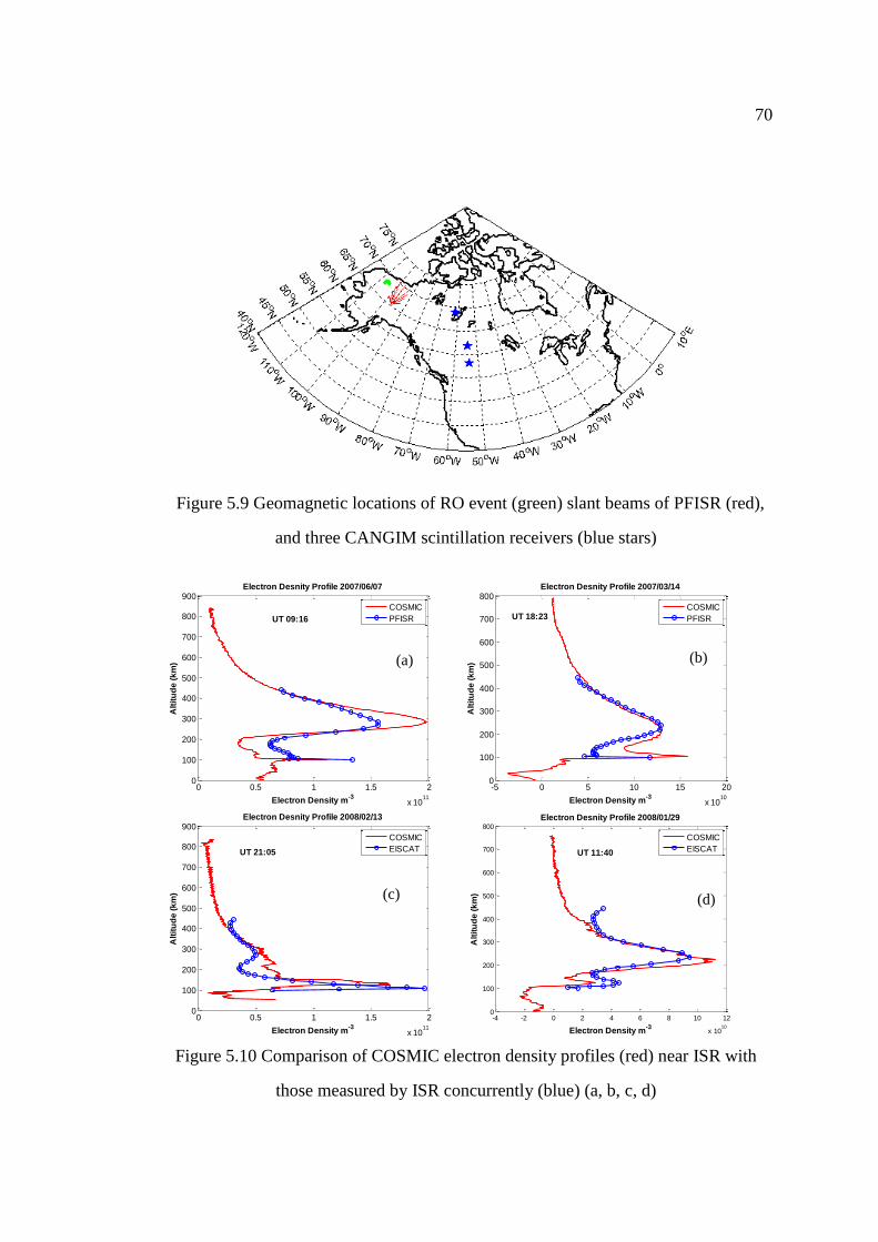
70
Figure 5.9 Geomagnetic locations of RO event (green) slant beams of PFISR (red),
and three CANGIM scintillation receivers (blue stars)
0 0.5 1 1.5 2
x 1011
0
100
200
300
400
500
600
700
800
900
Electron Density m-3
Alt
itu
de
(k
m)
Electron Desnity Profile 2007/06/07
COSMIC
PFISRUT 09:16
-5 0 5 10 15 20
x 1010
0
100
200
300
400
500
600
700
800
Electron Density m-3
Alt
itu
de
(k
m)
Electron Desnity Profile 2007/03/14
COSMIC
PFISRUT 18:23
0 0.5 1 1.5 2
x 1011
0
100
200
300
400
500
600
700
800
900
Electron Density m-3
Alt
itu
de
(k
m)
Electron Desnity Profile 2008/02/13
COSMIC
EISCATUT 21:05
-4 -2 0 2 4 6 8 10 12
x 1010
0
100
200
300
400
500
600
700
800
Electron Density m-3
Alt
itu
de
(k
m)
Electron Desnity Profile 2008/01/29
COSMIC
EISCATUT 11:40
Figure 5.10 Comparison of COSMIC electron density profiles (red) near ISR with
those measured by ISR concurrently (blue) (a, b, c, d)
(a) (b)
(c) (d)

71
However the values of AEI peak electron density are not identical for the two types of
observations, especially for case (c). It is noted that the RO events are not exactly
co-located with ISR observations. RO events do not occur coincidentally above the
ISR sites. And during nighttime auroral conditions the electron density irregularities
at 110 km altitude associated with AEI can be quite localized: the horizontal scale size
ranges from 20 to 400 km [Coker et al., 1995]. The geographic location of the RO ray
path tangent points for one RO event can change by several hundred kilometers
beginning (top) versus end (bottom) of the profile.
Therefore the differences between observations in the E region may arise from the
localized nature of the irregularity and location mismatch between the two types of
observations. The assumption of local spherical symmetry of electron density in a
large region could be another error source for RO inversion. This assumption
becomes inadequate under disturbed ionospheric conditions since horizontal
ionospheric gradients are present in the nighttime aurora.
There is also some disagreement in the Figure 5.10 COSMIC and ISR profiles at F
region altitudes. The most obvious case is (a) with NmF2 (density of F2 peak)
measured by COSMIC being about 0.4×10¹¹
el/m3 larger than the ISR measurement.
The HmF2 (altitude of F2 peak) is in good agreement with ISR data. And the profile
shape between the two measurements generally matches well. Other comparison
profiles are not shown here. Figure 5.11 provides the summary of comparisons with
ISR. Correlation of the electron density peak at AEI altitude is 0.78 for 28 events
selected during disturbed nighttime periods. Generally for all the cases COSMIC RO
electron density profiles are in agreement with those observed by ISR. Most
differences of measured AEI are within 0.5×10¹¹
el/m3 for the selected 28
cases.

72
0 0.5 1 1.5 2 2.5 3 3.5
x 1011
0
0.5
1
1.5
2
2.5
3
3.5x 10
11
COSMIC Peak Density of E layer (m-3
)
ISR
Pe
ak
De
ns
ity
of
E la
ye
r (m
-3)
Disturbed Aurora Night (2007~2008)
Corr = 0.78N = 28
Figure 5.11 Correlation between the COSMIC E region precipitation density and
those from ISR during disturbed auroral nighttime periods in 2007 and 2008
For the F region, comparisons do not show large differences for NmF2 or HmF2 (in the
published results by Lei et al. [2007], Hajj et al. [2000] and Hajj et al. [1998]). The
agreement of E region precipitation also appears to be good with the limited dataset.
For comparison of AEI at 110 km altitude, results show that the altitude of E layer
precipitation is generally well captured by COSMIC RO measurements. The
differences are the peak values between the two types of measurements, which could
result from the presence of non-constant horizontal gradients and spatial mismatch
between the two measurements. This deficiency of the Abel inversion is more
significant for disturbed ionospheric conditions. Overall agreements are obtained in
the selected AEI cases with correlation coefficient of 0.78.
5.3 VALIDATION BY IONOSONDE
Another common tool for ionosphere observation is the ionosonde. Lei et al. [2007]
conducted comparisons between the retrieved electron density peaks (NmF2) from
COSMIC observations and measurements from 31 globally distributed ionosondes. A

73
dataset of 276 coincident events were identified and validated for June 2006. All RO
events were required to be within 2° latitude and 2° longitude of the location of a
given ionosonde. The NmF2 electron densities were compared. The correlation result
is shown in Figure 5.12 with a correlation coefficient of 0.85. Hajj et al. [2000]
conducted another comparison of RO profiles with ionosondes. A dataset of 4111 RO
occultation events from GPS/MET were selected with tangent points within 1200 km
of the ionosonde location and within 1 hour period. A scatter plot of NmF2 correlation
is shown in Figure 5.13 (a) and a histogram of the differences in density (NmF2
(GPS/MET)-NmF2 (ionosonde)) is shown in Figure 5.13 (b).
Figure 5.12 Correlation between COSMIC NmF2 and ionosonde measurements for
July 1 to 31 2006 [after Lei et al., 2007]
Hajj et al. [2000] also analyzed the measurement differences as a function of local
time. Analysis showed that the fractional difference is larger during pre-dawn periods.
Since the spherical symmetry assumption is inadequate when the ionosphere is full of
irregularities and structures (which can introduce large errors to the electron density
retrieval by RO) the large fractional errors of NmF2 at night reflect that ionospheric

74
horizontal gradients are generally more significant at nightside.
Figure 5.13 (a) Correlation of 4111 coincident events between ionosondes and RO
from GPS/MET, and (b) Statistical analysis of the 4111 events [after Hajj et al., 2000]
Stratus [1999a; 1999b] reached a similar conclusion. Beyond using different
observation tools there have also been other analyses conducted: for example
comparisons between RO profiles that took place in close proximity. Please refer to
Hajj et al. [2004], Schreiner et al. [2007], Anthes et al. [2008] and Kuo et al. [2004].
5.4 VALIDATION SUMMARY
This chapter provided an overview of RO electron density profile validation. A dataset
of disturbed days was selected to validate the RO electron density profiles using ISR
observations. The limited datasets demonstrated an agreement between the two types
of observations. Under disturbed ionospheric conditions COSMIC RO can capture the
altitude of E region precipitation and provide realistic electron density profiles. The
presence of non-constant horizontal gradients and spatial and temporal mismatch
(a) (b)

75
between two measurements contribute to any major discrepancies. Syndergaard et al.
[2006] concluded that the largest error source for GPS RO electron density profile is
the strong horizontal gradients; assumptions made in the Abel inversion become less
valid with the existence of strong electron gradients in the ionosphere. Incorrect
assumptions can result in either positive or negative errors larger than 105 el/cm
3 at
the bottom of the retrieved profiles in certain cases [COSMIC, 2009]. A method to
overcome the horizontal inhomogeneity of the ionosphere is to include external
information during the inversion process [Kuo et al., 2004]. There is also ongoing
research to improve the retrieval algorithm [Hajj and Romans, 1998; Schreiner et al.,
1999]. For future work more extensive validation needs to be carried out for
“disturbed” electron density profiles.
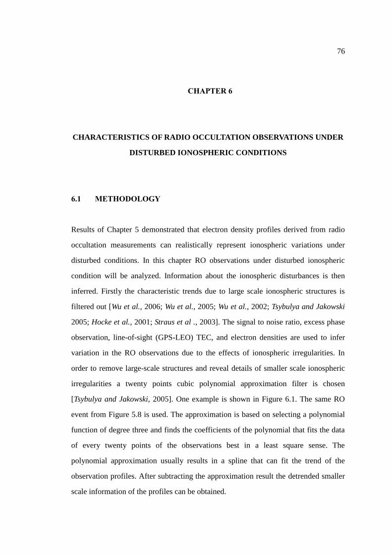
76
CHAPTER 6
CHARACTERISTICS OF RADIO OCCULTATION OBSERVATIONS UNDER
DISTURBED IONOSPHERIC CONDITIONS
6.1 METHODOLOGY
Results of Chapter 5 demonstrated that electron density profiles derived from radio
occultation measurements can realistically represent ionospheric variations under
disturbed conditions. In this chapter RO observations under disturbed ionospheric
condition will be analyzed. Information about the ionospheric disturbances is then
inferred. Firstly the characteristic trends due to large scale ionospheric structures is
filtered out [Wu et al., 2006; Wu et al., 2005; Wu et al., 2002; Tsybulya and Jakowski
2005; Hocke et al., 2001; Straus et al ., 2003]. The signal to noise ratio, excess phase
observation, line-of-sight (GPS-LEO) TEC, and electron densities are used to infer
variation in the RO observations due to the effects of ionospheric irregularities. In
order to remove large-scale structures and reveal details of smaller scale ionospheric
irregularities a twenty points cubic polynomial approximation filter is chosen
[Tsybulya and Jakowski, 2005]. One example is shown in Figure 6.1. The same RO
event from Figure 5.8 is used. The approximation is based on selecting a polynomial
function of degree three and finds the coefficients of the polynomial that fits the data
of every twenty points of the observations best in a least square sense. The
polynomial approximation usually results in a spline that can fit the trend of the
observation profiles. After subtracting the approximation result the detrended smaller
scale information of the profiles can be obtained.
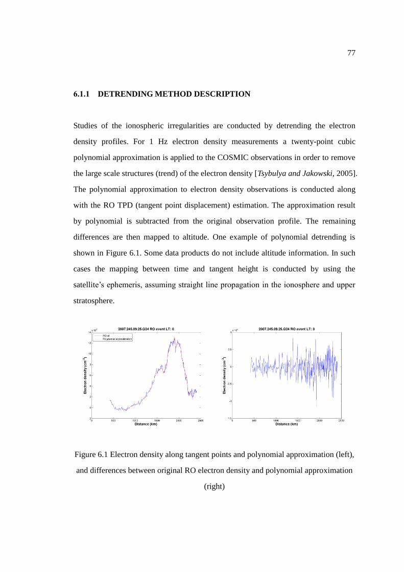
77
6.1.1 DETRENDING METHOD DESCRIPTION
Studies of the ionospheric irregularities are conducted by detrending the electron
density profiles. For 1 Hz electron density measurements a twenty-point cubic
polynomial approximation is applied to the COSMIC observations in order to remove
the large scale structures (trend) of the electron density [Tsybulya and Jakowski, 2005].
The polynomial approximation to electron density observations is conducted along
with the RO TPD (tangent point displacement) estimation. The approximation result
by polynomial is subtracted from the original observation profile. The remaining
differences are then mapped to altitude. One example of polynomial detrending is
shown in Figure 6.1. Some data products do not include altitude information. In such
cases the mapping between time and tangent height is conducted by using the
satellite’s ephemeris, assuming straight line propagation in the ionosphere and upper
stratosphere.
Figure 6.1 Electron density along tangent points and polynomial approximation (left),
and differences between original RO electron density and polynomial approximation
(right)

78
6.1.2 GENERAL CHARACTERISTICS OF AURORAL EVENTS
6.1.2.1 LOW FREQUENCY OBSERVATIONS
The local geomagnetic field on September 1 2007 indicated ionospherically disturbed
conditions in Alaska during 0800 to 1200 UT (refer to Figure 5.7) [GIMA, 2009]. One
RO event occurred at 0958 UT close to the GIMA magnetometer network (refer to
Figure 5.9). The COSMIC data products recorded in “ionPhs” and “ionPrf” files are
plotted and detrended for the selected RO event. Figure 6.2 from top to bottom shows
the GPS TEC measurement, C/A code SNR, L2 SNR, and electron density
measurements.
The SNR plots (Figure 6.2 (b) and (c)) and electron density profile (Figure 6.2(d))
show an obvious enhancement at 110 km altitude (E region). Measurements in Figure
6.2 start from a tangent height around 600 km. All the detrended plots show obvious
fluctuations at 110 km altitude corresponding to the AEI feature during auroral
nighttime. The decrease in C/A and L2 SNR indicates that AEI structures at 110 km
altitude are introducing amplitude scintillation for the LEO-GPS link. TEC and
density measurements both show an enhancement of ionospheric delay and
fluctuation in the E region. In this example SNR, raw observations, and retrieved
electron density exhibit good consistency with the expected altitude (110 km) of
ionospheric disturbances during AEI.

79
0 5 100
100
200
300
400
500
600
Alt
itu
de
(k
m)
TEC Measurement
TEC (TECU)
-0.5 0 0.50
100
200
300
400
500
600
Alt
itu
de
(k
m)
Detrended TEC
TEC (TECU)
(a)
200 300 400 5000
100
200
300
400
500
600
Alt
itu
de
(k
m)
C/A code
SNR (V/V)-100 0 1000
100
200
300
400
500
600
Alt
itu
de
(k
m)
Detrended Result
SNR (V/V)
(b)
0 100 2000
100
200
300
400
500
600
SNR (V/V)
Alt
itu
de
(k
m)
L2
-50 0 500
100
200
300
400
500
600
Alt
itu
de
(k
m)
SNR (V/V)
Detrended Result (c)
0 2 4 6
x 105
0
100
200
300
400
500
600
Electron Density (el/cm3)
Alt
itu
de
(k
m)
Electron Density Profile
-1 0 1
x 105
0
100
200
300
400
500
600Detrended Result
Electreon Density (el/cm3)
Alt
itu
de
(k
m)
(d)
Figure 6.2 COSMIC level 1 and level 2 products for 1 Hz RO observations on
September 1 2007 at 0958 UT (left) and the perturbation extracted from polynomial
approximation detrending (right) for (a) 1 Hz TEC measurements from L1 and L2
phase observation, (b) C/A code SNR, (c) L2 SNR, and (d) electron density profile

80
0 2 4 6
x 105
0
100
200
300
400
500
600
Electron Density(el/cm3)
Alt
itu
de
(k
m)
Electron Density Profile
-1 0 1
x 105
0
100
200
300
400
500
600Detrended Result
Electron Density(el/cm3)
Alt
itu
de
(k
m)
Figure 6.3 COSMIC electron density products for RO on 24 August 2007
Figure 6.3 shows RO observations on 24 August 2007. This is another event that
occurred close to an Alaskan magnetometer at local midnight. However August 24
was a magnetically quiet day with K indices (magnetic fluctuations) at College Alaska
being 0 for the period studied. The plot axes are the same as in Figure 6.2 (d). It is
observed that the F region peak density (HmF2) for both the “quiet” profile and the
“disturbed” profile occur near 250 km altitude with a maximum density magnitude of
105
el/cm3. It can be observed in Figure 6.3 that for altitudes lower than 100 km there
are some negative electron density values. In reality it is impossible to have negative
electron density values. The false density values arise from the increasing neutral
component for troposphere altitude range. Usually below 50 km altitude the bending
contributions from air/water are generally larger compared to electron density effects
[Wu et al., 2005]. Another factor to contribute the negative value of electron density is
the spherical symmetry assumption made for the Abel inversion [Lei et al., 2007].
However the altitude range being considered for ionosphere effects is usually above
90 km altitude. The negative values of electron density for lower altitude range can be
neglected for the study of this thesis.
The major difference between the “disturbed” (Figure 6.2) and “quiet” (Figure 6.3)
profiles is the sudden enhancement appearing at E region altitudes (approximately 110

81
km) for the disturbed profiles (which corresponds to AEI structure). The NmF2 in
Figure 6.2 is 1.2×10⁵
el/cm3 while the NmF2 in Figure 6.3 is a bit larger at 1.8×10
5
el/cm3. Considering that the quiet case shows the nominal electron density profile at
midnight, the enhancement associated with AEI is noted to start from 150 km altitude
downward in Figure 6.2 (d).
6.1.2.2 HIGH FREQUENCY OBSERVATIONS
As described previously 50 Hz RO measurements are only available from
approximately 150 km altitude due to satellite data payload concerns. Analysis of 50
Hz data is shown in Figure 6.4.
Figure 6.4 shows 50 Hz SNR and L1 and L2 phase measurements of the same
COSMIC event on 1 September 2007. Starting from a tangent height at around 130
km, 50 Hz data scans through the E region at a descending rate around 2.2 km/s. Here
the SNR can vary substantially from occultation to occultation [Wu et al., 2005]. In
this example the SNR is larger than 5000 and decreases below 30 km altitude because
of defocusing effects in the neutral atmosphere. The SNR exhibits abrupt variations at
tangent heights around 100 km indicating the existence of sharp ionospheric
structures in that region.
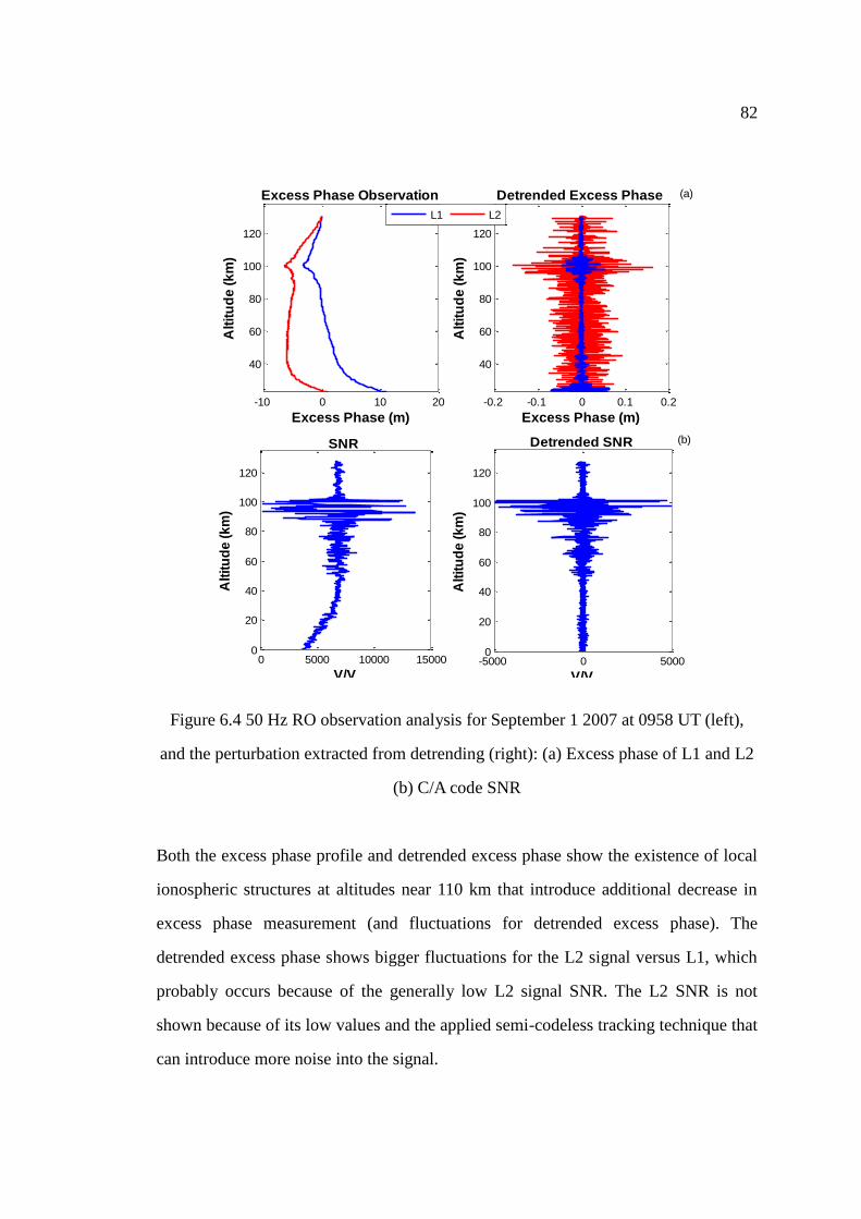
82
-10 0 10 20
40
60
80
100
120A
ltit
ud
e (
km
)
Excess Phase (m)
Excess Phase Observation
-0.2 -0.1 0 0.1 0.2
40
60
80
100
120
Alt
itu
de
(k
m)
Excess Phase (m)
Detrended Excess Phase
L1 L2
(a)
0 5000 10000 150000
20
40
60
80
100
120
Alt
itu
de
(k
m)
V/V
SNR
-5000 0 50000
20
40
60
80
100
120
Alt
itu
de
(k
m)
V/V
Detrended SNR (b)
Figure 6.4 50 Hz RO observation analysis for September 1 2007 at 0958 UT (left),
and the perturbation extracted from detrending (right): (a) Excess phase of L1 and L2
(b) C/A code SNR
Both the excess phase profile and detrended excess phase show the existence of local
ionospheric structures at altitudes near 110 km that introduce additional decrease in
excess phase measurement (and fluctuations for detrended excess phase). The
detrended excess phase shows bigger fluctuations for the L2 signal versus L1, which
probably occurs because of the generally low L2 signal SNR. The L2 SNR is not
shown because of its low values and the applied semi-codeless tracking technique that
can introduce more noise into the signal.

83
0 0.2 0.4 0.6 0.8 1
40
50
60
70
80
90
100
110
120
130
140
150
S4 index
Alti
tud
e (
km
)
Derived S4 scintillation index provided every second
Figure 6.5 S4 index provided by CDAAC (COSMIC)
Figure 6.5 shows the S4 index plot for the September 2007 event. The S4 index is
derived from the signal to noise intensity fluctuations in the raw 50 Hz L1 amplitude
measurements [Syndergaard, 2006]. It is used to show the amplitude scintillation of
RO signal received by LEO. In Figure 6.5 the scintillation is observed to be
significant at tangent heights in the E region due to the electron density irregularities
from AEI, which correspond to the same altitudes determined in previous analyses.
Both the 1 Hz and 50 Hz observations exhibit great agreement in identifying the
altitude of AEI occurrence. For scintillation studies of the high latitude region, the
auroral irregularity altitude and the intensity of signal fluctuation, as well as
correlation distance, are necessary in order to build three-dimensional phase screens
for ionosphere simulations.
6.1.3 DATA PROCESSING
The auroral E-ionization region is associated with large variations in electron density
at specific scale sizes. To extract small-scale structures of aurora the electron density

84
profile is detrended. The COSMIC level 1 product “ionPhs” is used to derive electron
density profiles by using University of Calgary in-house software. SNR, L1 and L2
raw observations are used from data recorded in “atmPhs” files. Disturbed periods are
selected based on a local magnetometer dataset or CANGIM scintillation observations
described in Section 5.1. The intensity and boundary of the aurora can be inferred
from the magnetometer observations. The CANGIM dataset is used to indicate the
presence of ionospheric scintillation (detected at ground locations). RO events are
selected during disturbed periods and within active ionosphere regions. Detrending
and power spectral density (PSD) analyses are applied to the “disturbed” RO
measurements to determine information about ionospheric instabilities in the high
latitude region. A flow chart of the whole process is shown in Figure 6.6.
Figure 6.6 Flow chart of data processing

85
In this thesis study the following processing and analyses are conducted by the
candidate.
The “disturbed” electron density profiles from the radio occultation
observations are selected based on CANGIM and magnetometer network
observations for the Canadian region.
Electron density profiles are detrended in order to remove the large-scale
components. Then the remaining small-scale perturbations are input for further
PSD analyses.
Altitude, scale size and intensity information of ionospheric irregularities is
derived. In future such information can be used for multi-phase screen
scintillation simulation modeling. However the modeling part is beyond the
scope of this thesis.
Figure 6.7 Vertical velocity for one RO observation with 1 Hz data rate in the
ionosphere at different altitudes

86
For PSD analysis, because radio occultation observations are not evenly sampled in
the spatial domain (shown in Figure 6.7), an alternative technique to the Fast Fourier
Transform named “Lomb method” is chosen. For the “Lomb method” [Lomb, 1976]
the power spectral density is derived from a least squares adjustment (fit) to each
discrete wave number.
6.1.4 AURORAL BOUNDARY PREDICTION
The aurora oval location is predicted using software developed at University of
Calgary. Predictions are computed using ground magnetometer data at different
latitudes, for example the CARISMA magnetometer line (from TALO station in the
north to PINA station in the south) [CSSDP, 2009]. Satellite-based observations for
auroral energy and GUVI (Global Ultraviolet imager) are also used as complementary
observations.
The fundamental method is described as follows. The magnetometers measure the
north-south component of the magnetic field (X), the east-west component (Y) and
the vertical component (Z). The three components are continuously measured. Once
the magnetic field becomes disturbed the east-west auroral electrojet current grows.
The dominant westward electrojet causes a decrease in the X component. The Z
component then gives the location of the boundary of the east-west currents; peaks in
the Z component are used to define the edges of the electrojet, which defines the
auroral boundary.
Evolution of the electrojet width and position for a certain longitude can be obtained
by using magnetometer observations at different latitudes along a meridian to profile
the auroral electrojet. The real-time auroral oval mapping is generated at

87
http://portal.cssdp.ca. Figure 6.8 shows the auroral boundary defined by the software
developed at University of Calgary.
Figure 6.8 Auroral boundary (blue) at 0830 and 1000 UT October 3 2007. The three
triangles show locations of CANGIM scintillation receivers.

88
Figure 6.9 Phase scintillation observations at CANGIM site Yellowknife,
October 3 2007
Phase scintillation observations at Yellowknife are shown in Figure 6.9 and used to
validate the presence of ionospheric scintillations. The red points indicate values
larger than 0.1 rad. At 0830 UT some severe scintillation is observed. In Figure 6.8
the location of Yellowknife is in the middle of the auroral oval. At 1000 UT there are
no large phase scintillation values observed in Figure 6.9. Accordingly in Figure 6.8
the auroral oval is at higher latitudes (poleward of Yellowknife). This is a simple
example to exhibit the correlation between auroral phenomenon and phase
scintillation observed at ground sites. In the analyses conducted here both
magnetometer measurements and CANGIM observations are used to identify
disturbed ionospheric conditions. Electron density profiles and other RO
measurements are then selected according to the ground observations to demonstrate
the in situ ionospheric characteristics during high-latitude ionospherically disturbed
conditions.
6.1.5 EVENT SELECTION
As mentioned previously RO events are selected for ionospherically disturbed
conditions with tangent points located within auroral boundaries during periods with

89
ground scintillation effects observed by CANGIM. Events are specified for two types
of ionospheric phenomena: aurora during substorm periods and SED for major
magnetic storms.
6.2 HIGH LATITUDE RADIO OCCULTATION EVENTS UNDER
IONOSPHERICALLY DISTURBED CONDITIONS
6.2.1 EVENT ANALYSES
In this section high-latitude electron density profiles retrieved from RO observations
are studied; data are selected based on ground observations (phase scintillations and
magnetometer data) under disturbed ionospheric conditions. A substorm on October 1
2007 and the severe storm period on October 29, 2003 are chosen. Corresponding RO
events are selected to investigate the irregularity intensity and distribution during high
latitude ionospherically disturbed times.
6.2.1.1 AURORAL EVENTS
Two events are selected for auroral substorm periods, as detected by magnetometer
observations, in which RO observations are available at auroral oval latitudes. The
tangent points of RO profiles are shown as blue lines in Figure 6.10. CANGIM
scintillation ionospheric pierce points (IPP) are also shown in green (moderate phase
scintillation in the range 0.2-0.5 rad) and red (strong phase scintillation larger than 0.5
rad) [Yu, 2007].

90
Figure 6.10 Two cases of COSMIC RO events with tangent points inside the auroral
oval during disturbed nighttime conditions, with trajectory of tangent points (blue)
and CANGIM scintillation observation larger than 0.5 rad (red) and between 0.2 rad
and 0.5 rad (green)
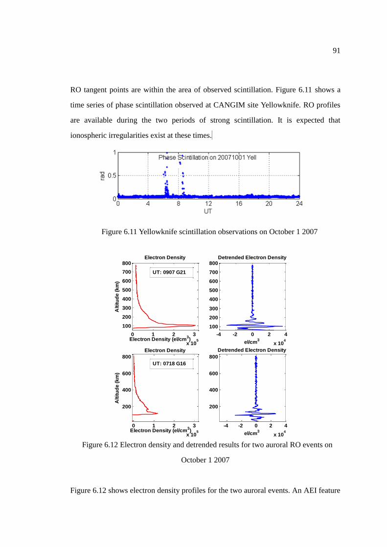
91
RO tangent points are within the area of observed scintillation. Figure 6.11 shows a
time series of phase scintillation observed at CANGIM site Yellowknife. RO profiles
are available during the two periods of strong scintillation. It is expected that
ionospheric irregularities exist at these times.
Figure 6.11 Yellowknife scintillation observations on October 1 2007
0 1 2 3
x 105
100
200
300
400
500
600
700
800
Electron Density (el/cm3)
Alt
itu
de
(k
m)
Electron Density
-4 -2 0 2 4
x 104
100
200
300
400
500
600
700
800
el/cm3
Detrended Electron Density
UT: 0907 G21
0 1 2 3
x 105
200
400
600
800
Electron Density (el/cm3)
Alt
itu
de
(k
m)
Electron Density
-4 -2 0 2 4
x 104
200
400
600
800
el/cm3
Detrended Electron Density
UT: 0718 G16
Figure 6.12 Electron density and detrended results for two auroral RO events on
October 1 2007
Figure 6.12 shows electron density profiles for the two auroral events. An AEI feature
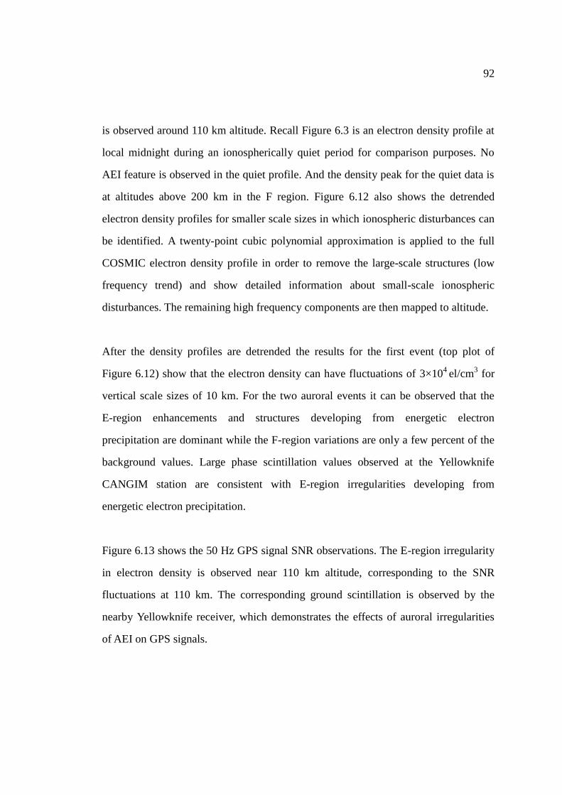
92
is observed around 110 km altitude. Recall Figure 6.3 is an electron density profile at
local midnight during an ionospherically quiet period for comparison purposes. No
AEI feature is observed in the quiet profile. And the density peak for the quiet data is
at altitudes above 200 km in the F region. Figure 6.12 also shows the detrended
electron density profiles for smaller scale sizes in which ionospheric disturbances can
be identified. A twenty-point cubic polynomial approximation is applied to the full
COSMIC electron density profile in order to remove the large-scale structures (low
frequency trend) and show detailed information about small-scale ionospheric
disturbances. The remaining high frequency components are then mapped to altitude.
After the density profiles are detrended the results for the first event (top plot of
Figure 6.12) show that the electron density can have fluctuations of 3×10⁴
el/cm3 for
vertical scale sizes of 10 km. For the two auroral events it can be observed that the
E-region enhancements and structures developing from energetic electron
precipitation are dominant while the F-region variations are only a few percent of the
background values. Large phase scintillation values observed at the Yellowknife
CANGIM station are consistent with E-region irregularities developing from
energetic electron precipitation.
Figure 6.13 shows the 50 Hz GPS signal SNR observations. The E-region irregularity
in electron density is observed near 110 km altitude, corresponding to the SNR
fluctuations at 110 km. The corresponding ground scintillation is observed by the
nearby Yellowknife receiver, which demonstrates the effects of auroral irregularities
of AEI on GPS signals.
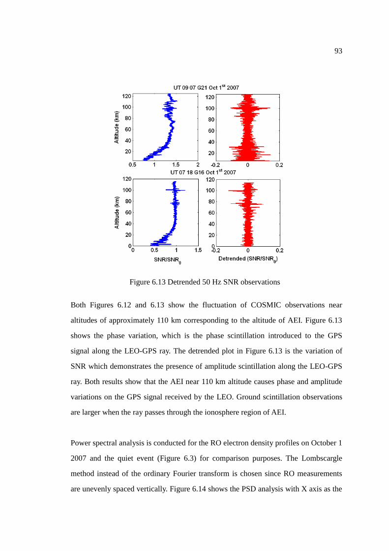
93
Figure 6.13 Detrended 50 Hz SNR observations
Both Figures 6.12 and 6.13 show the fluctuation of COSMIC observations near
altitudes of approximately 110 km corresponding to the altitude of AEI. Figure 6.13
shows the phase variation, which is the phase scintillation introduced to the GPS
signal along the LEO-GPS ray. The detrended plot in Figure 6.13 is the variation of
SNR which demonstrates the presence of amplitude scintillation along the LEO-GPS
ray. Both results show that the AEI near 110 km altitude causes phase and amplitude
variations on the GPS signal received by the LEO. Ground scintillation observations
are larger when the ray passes through the ionosphere region of AEI.
Power spectral analysis is conducted for the RO electron density profiles on October 1
2007 and the quiet event (Figure 6.3) for comparison purposes. The Lombscargle
method instead of the ordinary Fourier transform is chosen since RO measurements
are unevenly spaced vertically. Figure 6.14 shows the PSD analysis with X axis as the

94
wave number. For each event the top plot is the power spectral analysis with wave
number less than 0.05 km-1
. The electron density profile for the quiet day (blue line) is
dominated by one major peak at 0.0025 km-1
which corresponds to a wavelength of
approximately several hundred kilometers.
0 0.01 0.02 0.03 0.04 0.050
50
100
150
Po
we
r
PSD Analysis of Electron Density Profile from COSMIC
0.05 0.1 0.15 0.2 0.25 0.30
5
10
15
Wavenumber (km-1
)
Aurora ED Profile (UT 0718 G16)
Quiet ED Profile
PSD after Filter
0 0.005 0.01 0.015 0.02 0.025 0.03 0.035 0.040
50
100
150
Po
we
r
0.05 0.1 0.15 0.2 0.25 0.30
5
10
15
Wavenumber (km-1
)
Aurora ED Profile (UT 0907 G21)
Quiet ED Profile
PSD after Filter
Figure 6.14 Power spectral analyses of electron density profiles for the two selected
auroral events
The blue line is the quiet event (from Figure 6.3) for comparison purposes. From
analysis of the two events it can be expected that structures with scale sizes of 50-100
km have peak power in the disturbed profile. The bottom plot of each event is the
PSD for small wavelengths. Only structures with scale sizes less than 30 km remain.

95
Two obvious peaks around 0.05 km-1
wave number (corresponding to a wavelength of
20 km) are observed for the “auroral” electron density profiles. In reality the PSD
analysis of ionospheric structures is limited by the vertical resolution of RO
measurements. There is no significant difference for wavelengths less than 10 km
between “auroral” and quiet electron density profiles. The conspicuous peak at 20 km
wavelength (red line) may arise from the enhanced E region at 110 km with vertical
scale size of tens of kilometers.
An autocorrelation function is calculated for the two “auroral” electron density
profiles and the quiet profile. In Figure 6.15 the correlation distances for the two
auroral events are much smaller compared with the quiet profile, which mainly comes
from the structure of electron precipitation in the E region. The sharp and thin layer
with sudden enhancement near 110 km also comprises small scale electron density
irregularities. Signals transmitted by satellite navigation systems will experience
strong scintillation effects due to the instabilities in this thin layer. The autocorrelation
function also reveals that the thickness of AEI is approximately tens of kilometers,
while the correlation coefficient drops to 0.5 at around 20 km wavelength.
0 200 400 600 800 10000
0.5
1
Wavelength (km)
Autocorrelation Function
Aurora ED UT 0907 G21
Quiet ED
Aurora ED UT 0718 G16
Figure 6.15 Autocorrelation function for the two “auroral” electron density profiles
and the quiet profile

96
Wavelet powerspectrum analysis is also applied to study the three electron density
profiles in Figures 6.16 and 6.17. Wavelets can be solved with a flexible resolution for
the spectrum in both frequency and time domains. For RO observations the spectrum
is mapped into altitude and wave number domain. Here the popular “Morlet” wavelet
is chosen as the mother wavelets. A filled contour plot is used to visualize the
powerspectrum [Trauth, 2007].
Altitude (km)
Waven
um
ber
(km
-1)
2007 Oct 1 st
09 07 G21
100 200 300 400 500 600 700
0.01
0.02
0.03
0.04
0.05
0.06
0.07
0.08
0.09
A l t i t u d e ( k m )
Wa
ve
nu
mb
er
(
km
-1)
2 0 0 7 O c t 1 st
07 18 G16
100 200 300 400 500 600 700
0.01
0.02
0.03
0.04
0.05
0.06
0.07
0.08
0.09
Figure 6.16 Wavelet power spectrum analysis for the electron density profiles in
auroral region

97
The reason why wavelet method has been chosen to analyze electron density profiles
is the benefit of providing power distribution in both the time and frequency domains.
For the dataset studied here the power can be related to both the wavelength range and
altitude. And it is preferable to know the altitude for different scale sizes; this
information is not provided by normal Fast Fourier transform. Another advantage of
wavelet analysis compared with Fast Fourier transform is that it is advantageous to
resolve power distribution for functions which have discontinuities and are
non-periodic [Trauth, 2007]; this is directly applicable to the COSMIC electron
density profiles.
Power for the two “auroral’ event electron density profiles is mainly concentrated
from 100 km to 150 km altitude which reflects the E-region fluctuations. There is
high power at 110 km for both of the power spectrums. For the event at 0907 UT the
corresponding dominant wavelength is 50-100 km. For the 0718 UT event one
wavelength is dominant in the range 30-50 km. Both of the high-power regions are
associated with the sudden enhancement of electron precipitation in the E region
during disturbed auroral periods. Wavelets can be used to determine the altitudes of
such structures. Dominant effects are observed at 110 km altitude. In contrast for the
wavelet power spectrum of the quiet event in Figure 6.17, the power is mainly
concentrated in wavelengths larger than 200 km.
It is noted that the scale sizes determined in both the PSD analysis and the
autocorrelation calculations do not necessarily represent the real scale sizes of
ionospheric irregularities (which may be smaller in scale and below the resolution
threshold for the observation sample rate). However the observed electron density
variations (obtained by detrending or by wavelet analyses) are primarily associated
with plasma irregularities. In comparison with the power spectrum (Figure 6.17) of

98
the “quiet” electron density profile (Figure 6.3), more power can be found within
smaller wavelength ranges for disturbed events which is consistent with the existence
of small instabilities during high levels of ionospheric activity. The wavelet analysis
of COSMIC RO electron density shows good correlation of irregularities for altitude
ranges determined from the detrending analysis.
Altitude (km)
Waven
um
ber
(km
-1)
2007 Oct 24 th
13 06 G20
100 200 300 400 500 600 700
0.01
0.02
0.03
0.04
0.05
0.06
0.07
0.08
0.09
Figure 6.17 Wavelet power spectrum analysis for the quiet electron density profile
1306 UT (G20) on October 24 (the corresponding density profile is shown in Figure
6.3)
6.2.1.2 EXTREME STORM EVENTS
Amplitude scintillation is not common for high latitudes. However, during an extreme
storm on October 29 2003 amplitude scintillation was recorded in CANGIM
observations. Two RO events from CHAMP were identified with ground amplitude
scintillation observed by CANGIM (Figure 6.18). The S4 index and phase
scintillation index at Yellowknife is shown in Figure 6.19. Phase scintillation reached
high values of 1 rad which is considered to be severe scintillation.

99
Figure 6.18 Two COSMIC RO events during the severe storm on October 29 2003
and phase scintillations observed by CANGIM with threshold of 0.5 rad (red), and
between 0.2 rad and 0.5 rad (green)

100
Figure 6.19 Yellowknife scintillation observations on October 29 2003
Electron density profiles for the two CHAMP RO events are shown in Figure 6.20.
From the raw density and detrended results it is observed that both profiles show large
E region enhancements and fluctuations extending to the F region. The electron
densities are generally larger than those observed in other events (in previous
sections). The events shown in Figure 6.20 are for the daytime sector (with solar
radiation creating more electron density). Also, on October 29 2003 (during the storm
period), the ionosphere was severely disturbed with the presence of SED causing
large gradients and density enhancements.
Both events occurred at the time and location consistent with amplitude scintillation
observed at ground CANGIM receivers. Amplitude scintillation at L-band is not as
common for high latitude regions as phase scintillation. However, during severe storm
periods the entire ionosphere is disturbed with small-scale structures distributed over
a range of altitudes and irregularities at a wide range of scale sizes. Radiowaves, after
propagating through the ionosphere, will experience multiple effects from the
irregularities at different altitudes, resulting in both phase variations and SNR
variations.

101
1 2 3
x 105
100
150
200
250
300
350
400
Electron Density (el/cm3)
Alt
itu
de
(k
m)
Electron Density
-5 0 5
x 104
100
150
200
250
300
350
400
el/cm3
Detrended Electron Density
UT: 1931 G17
1 2 3
x 105
50
100
150
200
250
300
350
400
Electron Density (el/cm3)
Alt
itu
de
(k
m)
Electron Density
-5 0 5
x 104
50
100
150
200
250
300
350
400
el/cm3
Detrended Electron Density
UT: 2103 G18
Figure 6.20 Electron density and detrended results for CHAMP RO events on October
29 2003
In Figure 6.20 there is a larger altitude range of E-region fluctuations than for the
auroral electron density profiles shown previously. For altitudes above 150 km the
fluctuations are observed to fill the whole F region with higher fluctuations than for
normal profiles. Both the E- and F-regions generate more intense fluctuations than for
moderately disturbed events. In this analysis of two RO events it is noted that
scintillation models simulating SED effects must include electron density
irregularities for all ionospheric altitudes such that signals experience the cumulative
effect from all layers. In Figure 6.20 both of the density profiles have E-region
enhancements; however, there are more fluctuations in the F region for the event at
1931 UT. Power spectral density analyses are shown in Figure 6.21. Both events show
a peak at wavelengths in the range 10-20 km; this is also observed in the PSD of

102
auroral events for a wavelength of approximately 20 km. The power at the
corresponding 10-20 km wavelength could arise from the significant electron density
enhancement at 110 km. It is also noted that there are many spikes for 1931 UT event
with wavelengths less than 10 km; this is the result of F region density fluctuations.
Compared with the other events more power is observed in the small wavelength
range - corresponding to the F region small-scale irregularities at 1931 UT.
0 0.005 0.01 0.015 0.02 0.025 0.03 0.035 0.040
50
100
150
Po
we
r
0.05 0.1 0.15 0.2 0.25 0.30
5
10
15
Wavenumber (km-1
)
Oct 29th
(UT 1931 G17)
Quiet ED Profile
PSD after Filter
0 0.005 0.01 0.015 0.02 0.025 0.03 0.035 0.040
50
100
150
Po
we
r
0.05 0.1 0.15 0.2 0.25 0.30
5
10
15
Wavenumber (km-1
)
Oct 29th
(UT 2103 G18)
Quiet ED Profile
PSD after Filter
Figure 6.21 Power spectral analyses of electron density profiles for the two RO events
on October 29 2003. The blue line is the quiet event in Figure 6.3 for comparison
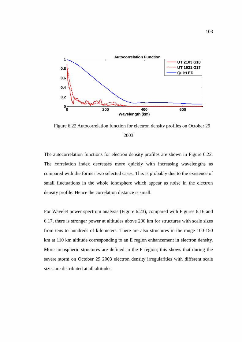
103
0 200 400 6000
0.2
0.4
0.6
0.8
1
Wavelength (km)
Autocorrelation Function
UT 2103 G18
UT 1931 G17
Quiet ED
Figure 6.22 Autocorrelation function for electron density profiles on October 29
2003
The autocorrelation functions for electron density profiles are shown in Figure 6.22.
The correlation index decreases more quickly with increasing wavelengths as
compared with the former two selected cases. This is probably due to the existence of
small fluctuations in the whole ionosphere which appear as noise in the electron
density profile. Hence the correlation distance is small.
For Wavelet power spectrum analysis (Figure 6.23), compared with Figures 6.16 and
6.17, there is stronger power at altitudes above 200 km for structures with scale sizes
from tens to hundreds of kilometers. There are also structures in the range 100-150
km at 110 km altitude corresponding to an E region enhancement in electron density.
More ionospheric structures are defined in the F region; this shows that during the
severe storm on October 29 2003 electron density irregularities with different scale
sizes are distributed at all altitudes.

104
Altitude (km)
Waven
um
ber
(km
-1)
2003 Oct 29 th
21 03 G18
100 200 300 400
0.01
0.02
0.03
0.04
0.05
0.06
0.07
0.08
0.09
Altitude (km)
Waven
um
ber
(km
-1)
2003 Oct 29 th
19 31 G17
100 200 300 400
0.01
0.02
0.03
0.04
0.05
0.06
0.07
0.08
0.09
Figure 6.23 Wavelet power spectrum analysis for the electron density profiles during
the severe storm on October 29 2003
6.3 SNR ANALYSIS
Figure 6.24 shows the SNR values for four RO events analyzed in previous sections
(two auroral events (a and b) and two profiles from the October 29 2003 storm (c and
d)).

105
0 200 400 6000
200
400
600
800
Alt
itu
de
(k
m)
SNR (V/V)
SNR (Oct 1st
G16 aurora event)
-40 -20 0 20 400
200
400
600
800 Detrended L1 SNR (a)
SNR (V/V)
L1 L2 L1
0 200 4000
200
400
600
800
Alt
itu
de
(k
m)
SNR (V/V)
SNR (Oct 1st
G21 aurora event)
-40 -20 0 20 400
200
400
600
800 Detrended L1 SNR (b)
SNR (V/V)
L1
0 500 1000
0
100
200
300
400
Alt
itu
de
(k
m)
SNR (V/V)
SNR (Oct 29th
G18 Storm event)
-40 -20 0 20 400
100
200
300
400 Detrended L1 SNR (c)
L1
0 200 400 6000
100
200
300
400
Alt
itu
de
(k
m)
SNR (V/V)
SNR (Oct 29th
G17 Storm event)
-40 -20 0 20 400
100
200
300
400 Detrended L1 SNR (d)
SNR (V/V)
L1
Figure 6.24 SNR and detrended L1 SNR (1 Hz sample rate) for the four events
under different ionospherically disturbed conditions

106
The SNR fluctuations for GPS radio occultation are caused by layered structures in
the ionosphere [Wu et al., 2005]. To extract high frequency (small-scale) SNR
perturbations the SNR data are detrended using a twenty point cubic polynomial
approximation filter. Results are shown in the figures on the right. For the two auroral
events the SNR fluctuates near 110 km. The G16 event also shows fluctuations
extending to 200 km; such variations were not apparent in the electron density
profiles. For the two SED RO events on October 29 2003 the SNR fluctuations are
very large in both E and F regions. Radio occultation observations on October 29
2003 are derived under more intense ionospheric disturbances than for the other two
cases. There are SNR fluctuations throughout all ionospheric altitudes for the 2003
storm events. SNR variations are introduced by ionospheric structures at a given
altitude.
Analysis of the SNR variance is one way to demonstrate effects of ionospheric
structures on satellite-based navigation system signals. Results show that AEI
structures during ionospherically disturbed periods are disruptive for the LEO-GPS
link. Under extreme storm scintillation conditions, fluctuations of satellite navigation
signals are caused by cumulative effects of structures distributed throughout the entire
ionosphere. SNR varies greatly in the disturbed E and F regions, and amplitude
scintillation of GPS signals occurs at high latitudes.
6.4 TEC CALCULATED FROM RAW OBSERVATIONS
In the previous validation it has been noted that the Abel inversion to retrieve electron
density profiles is inadequate due to the assumption of spherical symmetry during
disturbed periods. The assumption is inadequate because of the existence of localized

107
irregularities and gradients. In this section the analyses are redone using TEC along
the GPS-LEO line of sight for the same events considered previously. TEC is the total
electron content measurement along the LEO-GPS line-of-sight. It is measured by
using GPS L1 and L2 raw phase observations. TEC is mapped to the tangent point
altitudes to create the profiles. TEC values from phase measurements are relative TEC.
It is therefore assumed that the TEC series starts at a value of zero.
Figure 6.25 TEC profiles as a function of tangent points (left) and detrended results
(right) for four events analyzed previously
TEC computed from raw observations shows the vertical distribution of electrons.
Peaks are observed in Figure 6.25 at E-region altitudes for the two auroral events (a

108
and b). For the detrended TEC the vertical distribution of fluctuations shows almost
the same characteristics as analyses of the electron density profiles. For the two events
on October 29 2003 (c and d) the F-region fluctuations are larger than for the other
two events; this is likely the cause of amplitude scintillation observed at ground GPS
receivers. Wavelet analyses of the four TEC profiles are shown in Figure 6.26. The
top two events (a and b) on October 1 2007 are COSMIC RO events with tangent
points in the auroral region. Power is distributed mainly in the altitude range 100-150
km. Events on October 29 (c and d) are CHAMP RO observations during the severe
storm period. The power is distributed from the E region to above 200 km altitude;
this shows features similar to those derived for wavelet analyses of the electron
density profiles.
Figure 6.26 Wavelet power spectrum analysis for TEC profiles
This chapter applies PSD analysis to analyze radio occultation measurements under
disturbed ionospheric conditions. Information is obtained about the ionosphere
(a) (b)
(c) (d)

109
vertical structures’ scale size, spatial distribution and intensity. The AEI electron
density profiles show fluctuations around 110 km and SED events show the
fluctuation for the whole altitude range (E plus F regions). The observed results are
generally in accordance with known physical processing controlling the high latitude
plasma. The analyses not only provide information about ionosphere irregularity
distribution at high latitude but also demonstrates the potential of RO for ionosphere
monitoring of disturbed conditions.

110
CHAPTER 7
MAPPING OF HIGH-LATITUDE IONOSPHERIC IRREGULARITIES USING
COSMIC OBSERVATIONS
7.1 OBSERVATION AVAILIBILITY
The goal of COSMIC is to provide approximately continuous 24 hours of local time
coverage globally [Lei et al., 2007]. However it is still not be achieved as described in
Section 4.2. Figure 7.1 is an example of the distribution of tangent points for RO
observations from five COSMIC LEO FORMOSAT-3 satellites over a two-hour
interval. The local time sector is 0000 to 0200. The geometry of COSMIC satellites
causes most of the RO events to occur in the western hemisphere (for the selected
two-hour local time period on September 2 2007). For studies in this thesis only days
with enough RO events in the high-latitude western hemisphere during local night
time (Canadian region) are chosen to create ionosphere maps.
Figure 7.1 Distribution of tangent points for COSMIC RO with observations in local
time sector 0000 to 0200 September 2 2007

111
Figure 7.2 Averaged electron density map with observations from different longitude
sectors (150° W - 160° W) (top) and (60° W - 160° W ) (bottom), September 2 2007
Figure 7.2 is another example showing the observation availability for the selected
time period from Figure 7.1. Figure 7.2 shows electron density observations from

112
COSMIC RO mapped to geomagnetic latitude and altitude. The top plot only uses
observations averaged over 10 degrees of longitude while the bottom plot includes
observations in the extended sector of the western hemisphere from 60 deg to 160 deg.
RO events at different longitudes are mapped into the same latitude and altitude grid.
The map is therefore an average latitude and altitude distribution of electron density
in a given longitude sector for the high-latitude western hemisphere. Bins with no
values available are shown as white pixels. It is noted that ionospheric activity levels
were high on September 2 2007; the geomagnetic K index (Alaska) was greater than 5
for the period studied [NOAA, 2009].
It is noted that RO observations are undersampled in the Alaska longitude sector due
to the geometry of COSMIC satellites. In order to create full maps observations are
chosen from a wider longitude sector (60 deg W to 160 deg W) with ionospheric
activity levels inferred from magnetometer observations in GIMA, CARISMA, and
GSC networks. Magnetic time series from Alaska (GIMA) and the other two networks
show significant magnetic field fluctuations in the local time range 0000 to 0400 LT
on this day [GIMA, 2009; GSC, 2009; CARISMA, 2009]. An electron density
enhancement in the geomagnetic latitude range 60-80 deg N is observed near 110 km
altitude in Figure 7.2 for the two-hour local time sector.
A similar map is generated in Figure 7.3 with observations from December 8 2007
which is a magnetically quiet day for comparison purposes. The planetary Kp index
was zero for the entire quiet day [NOAA, 2009]. In contrast to the bottom plot of
Figure 7.2, no large E-region electron density enhancement exists. Typical F-region
electron density peaks are observed. In the previous example (Figure 7.2) E-region
electron density enhancements observed from COSMIC RO observations are
consistent with patterns of energetic electron precipitation expected for auroral
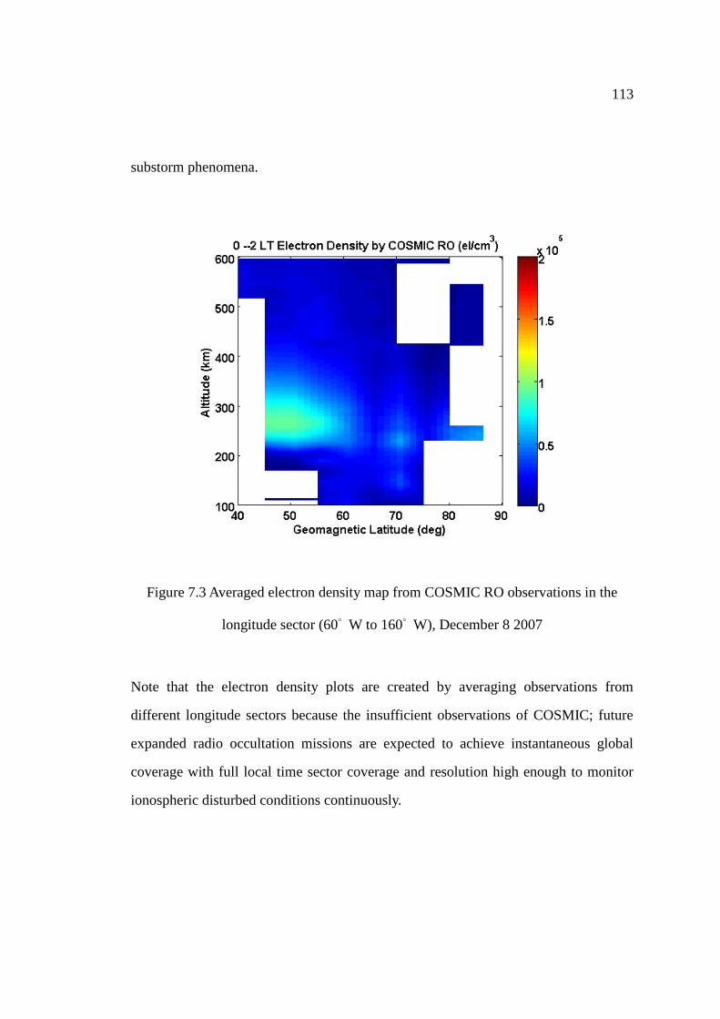
113
substorm phenomena.
Figure 7.3 Averaged electron density map from COSMIC RO observations in the
longitude sector (60° W to 160° W), December 8 2007
Note that the electron density plots are created by averaging observations from
different longitude sectors because the insufficient observations of COSMIC; future
expanded radio occultation missions are expected to achieve instantaneous global
coverage with full local time sector coverage and resolution high enough to monitor
ionospheric disturbed conditions continuously.

114
7.2 ANALYSES OF DISTURBED IONOSPHERE
7.2.1 ANALYSIS OF AURORAL EVENTS
Four successive ionospherically active nights were observed December 4 to 7 2008.
In Figure 7.4 magnetometer observations between 1000 and 1200 UT in Alaska show
decreases in the H (north-south) magnetic component consistent with the presence of
an enhanced westward electrojet - and auroral substorm events. Based on GIMA
observations in Figure 7.4 it can be determined that the ionosphere is disturbed
1000-1200 UT; this corresponds to 0000-0200 LT in Alaska.
Figure 7.4 Geomagnetic field measured at Poker Flat December 4 to 7 2008, [GIMA,
2009]

115
COSMIC measurements are selected for this four-day period. Figure 7.5 is derived
from such observations for the period 0400 to 2000 UT for the four days. COSMIC
electron density observations within the same longitude and same latitude sector are
compiled and averaged in a grid. The electron density observations are selected in the
altitude range 100 km to 120 km corresponding to the altitude of AEI.
Figure 7.5 COSMIC electron density observations for altitude range 100-120 km
generated from COSMIC measurements every two-hour time sector from 0400 to
2000 UT, as averaged over four days (December 4 2008 to December 7 2008) in
geomagnetic coordinates
In Figure 7.4 magnetometer observations indicate that 1000 to 1200 UT is the most
disturbed period for each of the four days. Accordingly in Figure 7.5 the E-region

116
electron density is enhanced at 60° W and 90° W geomagnetic longitude, which
illustrates significant electron precipitation in the ionospheric E region near Alaska.
Except the major decrease period of H component of magnetic field in Figure 7.4 two
additional periods of geomagnetic fluctuations (0600-0800 UT and 1600-1800 UT)
are also observed on December 5 and 6. Correspondingly the electron density is
enhanced near Alaska (90° W) in Figure 7.5 for these two periods. The correlation
between geomagnetic variations and electron density enhancement reflects the nature
of the physical processes. The auroral electrojet current grows (causing a negative
magnetic field perturbation) during the precipitation of energetic electrons into the
E-region along magnetically field-aligned currents (refer to Section 3.2.2.1).
7.2.2.1 CO-LOCATED ELECTRON DENSITY PROFILES
Electron density profiles are compared for different levels of ionospheric activity.
Figure 7.6 shows profiles for December 3 and 4, and December 7 and 8 2008. Note
that December 7 and December 4 are ionospherically disturbed days and December 3
and 8 are quiet days. The GPS satellite orbital period is approximately 12 hours; the
COSMIC LEO satellite orbital period is approximately 100 min. A RO event can
happen at almost the same location but 20-30 min earlier for a given COSMIC
LEO-GPS pair on successive days. Co-located electron density profiles are derived
from such observations to determine the ionospheric variations introduced by
substorm effects.

117
80oW 40oW 0o 30oN
50oN
70oN
90oN
0 1 2 3
x 105
0
200
400
600
800(a)
3 Dec UT 1027
4 Dec UT 0959
80oW 40oW 0o 30oN
50oN
70oN
90oN
0 1 2 3
x 105
200
400
600
800(b)
3 Dec UT 1046
4 Dec UT 1021
Ge
om
ag
ne
tic L
atitu
de
(D
eg
)
80oW 40oW 0o 30oN
50oN
70oN
90oN
0 1 2 3
x 105
0
200
400
600
800
Altitude (
km
)
(c)
3 Dec UT 1120
4 Dec UT 1055
80oW 40oW 0o 40oE
30oN
50oN
70oN
90oN
0 5 10
x 104
0
200
400
600
(d)
3 Dec UT 0952
4 Dec UT 0921

118
80oW 40oW 0o 30oN
50oN
70oN
90oN
0 2 4 6 8
x 104
100
200
300
400
500(e)
Electron Density (cm-3
)
8 Dec UT 1040
7 Dec UT 1102
Geomagnetic Longitude (Deg)
Figure 7.6 Five co-located pairs of COSMIC electron density observations (right)
during ionospherically disturbed days (red line for December 4 and 7) and quiet days
(blue line for December 3 and 8). Trajectories of RO tangent points are shown in
maps (left) (blue dots correspond to the blue profiles on the right and red dots
correspond to the red profiles on the right)
Figure 7.6 shows comparisons of five pairs of co-located COSMIC RO events for
quiet versus disturbed periods with one day difference. Events in plot (a) occur at
latitudes less than 60° geomagnetic, which is likely equatorward of the auroral oval.
The two plots in figure (a) match quite well, with an F-region electron density peak
typical of average ionospheric conditions; it can be inferred that ionospheric storm
conditions are minimal in this latitude sector for the dates considered. Other plots ((b)
to (e)) occur at relatively higher geomagnetic latitudes. The disturbed electron density
profiles show obvious E region enhancements compared with co-located quiet density
profiles. Plots (b), (c) and (e) also show local electron density peaks in the F region
(200-300 km) compared with quiet day profiles.
From these observations, the AEI enhancement is determined to occur within 10-20
km of 110 km altitude with a magnitude up to 105el/cm
3. The maximum F region
enhancement at altitudes 150-300 km is 5×10⁴ el/ cm
3. There are no major differences

119
for the disturbed versus quiet profiles at altitudes higher than 300 km. From this
example (Figure 7.6) electron density variations introduced by ionospheric storm
effects can be summarized as 1) significant AEI near 110 km altitude with 10-20 km
vertical scale, and 2) relative enhancement at F region at altitudes 150-300 km.
7.2.2.2 DENSITY MAPS FOR DIFFERENT ALTITUDES
Magnetometer observations between 1000 and 1200 UT in Alaska show decreases in
the H component in Figure 7.4. Disturbed ionosphere periods are also selected using
other high latitude magnetometer stations. Based on magnetometer observations of
the entire Canadian region, corresponding COSMIC RO measurements have been
selected during the period 4-7 December 2008. Spatial distribution and periods of
disturbances are identified using GIMA, CARISMA and GSC data. Figure 7.7 is
derived from the selected electron density observations at altitudes 100-120 km (top)
and other altitude ranges for night time sectors of the four days. Four days of
observations are included because there are not enough COSMIC RO measurements
for a single day to create a full electron density map. A plot is compiled from all
electron density measurements during disturbed periods for the given interval of local
time. COSMIC electron density observations within the same geomagnetic latitude
and local time sector bins are averaged to derive the grid of values in Figure 7.7.
The top plot is electron density observations selected for altitudes 100-120 km
(corresponding to the altitude of AEI). In that plot all density enhancements generally
occur above geomagnetic latitude 60 deg N; this is near the equatorward boundary of
the auroral oval. Localized electron density enhancements are from 2-3 ×10⁵ el/cm
3.
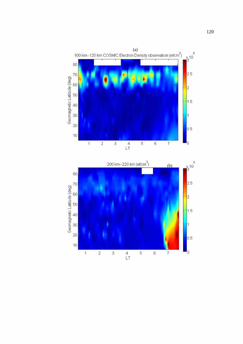
120
(a)
(b)

121
Figure 7.7 COSMIC electron density observations for altitude ranges (top to bottom)
(a) 100-120 km, (b) 200-220 km, (c) 300-320 km, and (d) 400-420 km, generated
from COSMIC measurements 0000-0800 LT for four days (4-7 December 2008)
(c)
(d)
122
For the plot of electron density at 200 km altitude F-region enhancements occur at
0700 LT which is before sunrise at the terminator location. The ionization starts at
lower latitudes around 0600 to 0700 local time as the sun rises. The enhancement of
density is from the beginning of ionization of a new day. For 300 km and 400 km
altitudes the density maps do not show obvious enhancement at auroral latitudes. It is
also observed that there is enhancement of electron density at mid-latitudes for
F-region altitudes of 300 km after midnight. With observations of electron density in
the altitude range 100-120 km the significant density enhancement is captured. The
correlation between magnetometer observations and spatial distribution of electron
density enhancement is consistent with the expected occurrence of AEI during
geomagnetic disturbances and associated auroral substorms. RO events from
COSMIC are able to capture the AEI feature from vertical electron density profiles
directly. The density at E region associated with AEI is comparable to the density of F
region during daytime, which is formed by the electron precipitation from the
field-aligned current.
A further comparison is made by plotting electron density maps compiled from
COSMIC measurements for quiet periods. Four quiet days from November 30 to
December 3 with geomagnetic K index being 1 or 0 for high latitude region are
identified. Observations of COSMIC RO for altitudes 100-120 km show no
significant electron density enhancement at auroral oval latitudes in Figure 7.8. The
F-region density enhancement near sunrise can still be observed for altitudes of
200-220 km. And the mid-latitude enhancement can be observed for 300 km altitude.
The major difference between disturbed density maps (Figure 7.7) and quiet maps
(Figure 7.8) for different altitude ranges is the high latitude density enhancement at
100 km for geomagnetically disturbed local nighttime - as associated with the auroral
activity.

123
Figure 7.8 COSMIC RO electron density observations for altitude ranges 100-120 km,
200-220 km, 300-320 km, and 400-420 km, as generated from COSMIC
measurements 0000-0800 LT for four days (November 30 to December 3 2008)
In order to show the electron enhancement of AEI feature more clearly, electron
density differences are calculated for different altitude ranges between quiet
observations in Figure 7.8 and disturbed observations in Figure 7.7. Figure 7.9 is
generated by using electron density measurements obtained from the four disturbed
days of Figure 7.7 subtracting density values in the grid with the same local time and
geomagnetic latitude of the quiet days of Figure 7.8. The largest differences are
observed in the top plot (100-120 km altitude) for the nighttime hemisphere; E-region
electron precipitation enhancement above 60° N can reach 3×10⁵ el/cm
3. For electron
density differences at 200 km, 300 km and 400 km altitude the values are not that
regular and found mainly for mid- and low-latitude regions. The ionosphere is also

124
active for mid- and low-latitude regions after local midnight and at sunrise due to
other ionospheric phenomena. However the results in Figure 7.9 show that for
different high-latitude altitude ranges the major difference is the enhancement around
100 km altitude associated with electron precipitation during auroral storm periods.
Figure 7.9 Electron density differences
between COSMIC measurements from
“disturbed” periods (December 4 to 7
2007) and “quiet” periods (November 30
to December 3) for different altitude
ranges (a to d)
(a)
(b) (c)
(d)
125
7.3 TEC MAPS
Figure 7.10 shows TEC estimates for the E and E-plus-F regions, as derived by
integrating COSMIC electron density with respect to altitude for observations from
the four ionospherically disturbed nights presented in previous sections. The top plot
shows total electron content integrated for the E-region altitude range 90-120 km
(corresponding to the AEI altitude). Good correlation can be found between TEC
enhancements and electron density enhancement 100-120 km altitude in Figure 7.7.
For the E region, enhanced TEC occurs in the geomagnetic latitude range 60-70 deg
N during local nighttime, which is mainly due to electron precipitation during storm
periods. The plot indicates that AEI can introduce TEC enhancements around 1 TECU
for the layer 90-120 km altitude; corresponding to 16 cm range delay for GPS L1
signals. Moreover the electron enhancement is not distributed symmetrically. AEI is
characterized by localized irregularity structures with large horizontal and vertical
gradients. AEI with horizontal scale sizes of dozens or hundreds of kilometers will
cause phase scintillation at high latitudes during auroral nighttime.
The bottom plot in Figure 7.10 shows TEC derived from integrated COSMIC electron
density profiles 90-600 km altitude from 0000 to 0800 LT. The obvious enhanced
TEC around 0600 and 0700 LT below 60° N is due to solar radiation (and ionization)
near the terminator. The enhanced TEC can also be observed at high latitudes above
60 deg N for 0100 to 0700 LT. The high-latitude enhanced TEC 90-600 km altitude
comes from the E-region electron precipitation (AEI - first plot in Figure 7.7) and also
F-region enhancement at 200 km altitude (second plot in Figure 7.7).
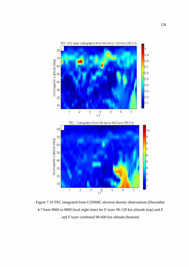
126
Figure 7.10 TEC integrated from COSMIC electron density observations (December
4-7 from 0000 to 0800 local night time) for E layer 90-120 km altitude (top) and E
and F layer combined 90-600 km altitude (bottom)
127
Differences between TEC measurements for quiet versus disturbed periods are shown
in Figure 7.11. TEC differences are calculated by subtracting quiet TEC values from
disturbed values for a given geomagnetic latitude and local time. Results are
computed for the E region 90-120 km altitude and E-plus-F region 90-600 km altitude;
only geomagnetic latitudes above 55 deg N are shown.
Figure 7.11 shows that E-region enhancement (due to AEI) during disturbed periods is
the main contributor to TEC measurement perturbations from the quiet ionosphere
values. The TEC enhancement associated with auroral periods is approximately 1
TECU from E region. And the density enhancement of AEI can extend to a wider
altitude range; the full TEC enhancement for altitudes 90-600 km can reach values of
1-3 TECU at the same location. For GPS applications the delay caused by structures
of AEI are from 0.15 meters to 0.45 meters for L1 frequency in addition to the normal
ionospheric range delay for enhancement from both the E and F region. From the
density observation comparison in Figure 7.6 there are still enhancements at 200 km
altitude at auroral latitudes that introduce TEC enhancement coming from F region
altitude.
Hunsucker et al. [1995] conclude that the occurrence of specific TEC signatures due
to large- and medium-scale E region structures can be utilized as the
predictor/monitor of AEI within the auroral oval. In Figure 7.6 comparisons disturbed
versus quiet conditions were conducted for single cases. The AEI enhancement can
reach to higher than 200 km altitude (plots b, c, e) for auroral density profiles. From
the analyses presented here TEC is expected to increase by 1-3 TECU for disturbed
versus quiet conditions. It can also be concluded that the AEI feature can have 1
TECU enhancement around 110 km altitude.

128
Figure 7.11 TEC differences between COSMIC measurements from “disturbed”
periods (December 4-7 2008) and “quiet” periods (November 30 to December 3 2008)
for different altitude ranges (90-120 km top plot, 90-600 km bottom plot) from 0000
to 0800 local time
129
Hunsucker et al. [1995] and Coker et al. [1995] determined that the AEI structures are
associated with 1 to 2 TECU change in TEC; this result was derived by applying a
filter to ground-GPS line-of-sight TEC observations. Such results are similar to the
results obtained in a different manner here by exploiting COSMIC RO capabilities.
COSMIC observations are used to estimate electron density profiles and identify TEC
perturbations in different altitude ranges. Analyses reveal dominant features of
ionospheric activity introduced in specific altitude ranges. Moreover it is observed
from COSMIC observations that the ionospheric structures are more extensive, and
distributed over a wide range of altitudes, than represented by a simple model of
ionospheric irregularities with assumption of one single phase screen. During auroral
substorms multiple phase screen modeling is necessary for realistic ionosphere
simulations in support of scintillation studies.
While the dataset used here is from solar minimum periods it is expected that the TEC
or electron density change could be more significant for storm events during solar
maximum periods (e.g. the severe storm in October 2003). GPS satellite signals may
experience degraded performance from ionospheric irregularities in local regions with
TEC enhancements introduced by auroral substorm effects. The additional range error
caused by the AEI structures can be associated with large horizontal TEC gradients
which also degrade the accuracy of safety-critical navigation systems such as the
Wide Area Augmentation System (WAAS).
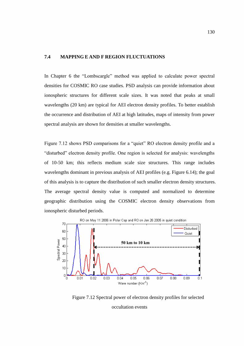
130
7.4 MAPPING E AND F REGION FLUCTUATIONS
In Chapter 6 the “Lombscargle” method was applied to calculate power spectral
densities for COSMIC RO case studies. PSD analysis can provide information about
ionospheric structures for different scale sizes. It was noted that peaks at small
wavelengths (20 km) are typical for AEI electron density profiles. To better establish
the occurrence and distribution of AEI at high latitudes, maps of intensity from power
spectral analysis are shown for densities at smaller wavelengths.
Figure 7.12 shows PSD comparisons for a “quiet” RO electron density profile and a
“disturbed” electron density profile. One region is selected for analysis: wavelengths
of 10-50 km; this reflects medium scale size structures. This range includes
wavelengths dominant in previous analysis of AEI profiles (e.g. Figure 6.14); the goal
of this analysis is to capture the distribution of such smaller electron density structures.
The average spectral density value is computed and normalized to determine
geographic distribution using the COSMIC electron density observations from
ionospheric disturbed periods.
Figure 7.12 Spectral power of electron density profiles for selected
occultation events
50 km to 10 km

131
Power spectral densities for electron density values in Figure 7.7 for the limited
wavelength range 10-50 km are shown in Figure 7.13. The results are normalized with
the maximum power set with value of 100.
Figure 7.13 PSD map for structures with scale sizes in the range 10-50 km for
electron density profiles derived from COSMIC measurements for ionospherically
active periods (December 4-7, time period 0100 to 0700 LT)
Larger values in Figure 7.13 demonstrate good correlation with the larger electron
density enhancements at altitudes 100-120 km in Figure 7.7 (first plot). Prominent
structures with scale size 10-50 km are observed within the auroral boundaries
defined in Figure 7.7. This implies that the occurrence of medium-scale structures
corresponds to the presence of nightside AEI. It is noted that there are also regions of
high spectral density at latitudes below the auroral oval boundary. However the
dominant distribution of medium-scale structures at auroral latitudes (and

132
corresponding to AEI) is evident. In addition to single PSD case studies in previous
sections, Figures 7.7 and 7.13 also show the direct correlation between E-region
density enhancements for disturbed auroral nighttime periods and PSD for structures
133
CHAPTER 8
CONCLUSIONS AND RECOMMENDATIONS
8.1 CONCLUSIONS
GPS radio occultation measurements onboard LEO satellites demonstrate potential as
a powerful tool for studying three-dimensional electron density in the high latitude
ionosphere. A drawback is that there are insufficient COSMIC RO events available
per day to achieve continuous global coverage. However, improved coverage can be
expected for COSMICII with an additional 12 satellites. Better spatial coverage can
be maintained for ionospheric tomography.
In Chapter 5 the validation of COSMIC electron density profiles during disturbed
periods is conducted and it is demonstrated that sufficient accuracy and resolution of
COSMIC electron density measurements can be achieved to capture and identify
small-scale ionospheric structures associated with scintillation. This work was
summarized in a poster presented at the COSMIC workshop (student poster
competition) in Boulder, USA, November 2009 [Feng and Skone, 2009].
Further analysis includes selection of a number of radio occultation events as
representative of disturbed auroral ionospheric conditions. Fluctuations in electron
density were observed near 110 km altitude during periods in which ground
scintillation was detected by CANGIM GPS receivers. For SED events the
ionospheric irregularities can extend into the F region over a wide range of altitudes.
134
Scale sizes of 10-20 km were observed for structures associated with AEI. For
analyses of electron density profiles during auroral events two conference papers have
been published [Skone et al., 2008; Skone et al., 2009].
Another important analysis conducted here is the derivation of electron density and
TEC maps for E-region disturbances with high resolution. Such maps showed the
spatial distribution of irregularities leading to scintillation effects; these products
could be made available to the GPS user community in an ionosphere warning system.
The auroral oval boundaries are readily apparent in these maps - essentially providing
a near real-time capability to track the evolution of auroral substorms. This work was
summarized in a presentation at the AMS conference held in Atlanta, USA, January
2010 [Feng and Skone, 2010]
A significant contribution of this work is identifying E-region electron density
enhancement signatures during auroral scintillation periods. From COSMIC
observations the presence of precipitating energetic electrons during auroral
substorms is identified at E-region altitudes; scintillations develop in such regions of
AEI processes. Results demonstrate that, for high latitude scintillation simulations (for
GNSS applications), a simple phase screen model assuming concentration of electrons
in a single thin layer is not realistic. A more complex multiple phase screen
physics-based model is required for realistic studies and simulations of high latitude
scintillation.
135
8.2 RECOMMENDATIONS
Radio occultation studies for the six-satellite COSMIC mission have provided new
capabilities to observe ionospheric structures. In this thesis analyses were conducted
for case studies of electron density profiles as well as ionosphere mapping on a global
scale. There are several recommendations for future research.
1. Validations of radio occultation electron density profiles with more truth
observations need to be conducted. Horizontal information about density distributions
is required to make the Abel inversion more accurate. Verification of COSMIC
electron density profiles especially for measurements of RO occurring at high
latitudes during ionospherically disturbed periods (confirmed with magnetometer
observations or ground scintillation measurements) should be conducted.
2. The RO electron density observations, or integrated TEC values, can also be used
to study the middle and low latitude ionospheric irregularities (e.g. spread-F
phenomenon, sporadic-E [Wu, 2006] and the effect of thermosphere wind shear). PSD
analysis can be used to determine presence of irregularity structures with different
scale sizes. Besides the raw observations from the LEO GPS receiver, L1 signal SNR
can be used to detect the existence of ionosphere irregularities.
3. With datasets from different RO missions and the upcoming solar maximum
period, long term observations can be used to study the annual and seasonal
ionospheric behavior.
4. RO measurements are able to provide information for ionosphere modeling or
scintillation modeling. The question of how to combine RO density profiles with
136
other observations (such as TEC measurements from ground-based GNSS receivers)
for data assimilation purposes, and how to simulate the electron density above LEO
altitudes, needs more consideration.
5. After COSMICII is deployed combinations of GPS, GLONASS, and other
navigation systems will be available. A continuous global coverage is expected for
better spatial resolution allowing ionospheric tomography. The detailed temporal
characteristics of ionospheric irregularities during storm periods can be derived.
GNSS RO are expected to provide capabilities for monitoring the ionosphere on a
large scale continuously to obtain the temporal and spatial correlation characteristics
of irregularities during disturbed conditions. Similar analyses of this study could be
implemented again with better ionospheric high latitude observation availability from
new RO missions.

137
REFERENCES
Aarons, J. (1993). The longitudinal morphology of equatorial F-layer irregularities
relevant to their occurrence. Space Science Reviews, vol. 63, issue 3-4, pp. 209-243.
Aarons, J. (1982). Global morphology of ionospheric scintillation. Proceedings of the
IEEE, vol. 70, pp. 360-378.
AMISR (2009). http://madrigal.haystack.mit.edu/, accessed on Aug 18, 2009
Anthes, R.A., P.A. Bernhardt, Y. Chen, L. Cucurull, K.F. Dymond, D. Ector, S.B.
Healy, S.P. Ho, D.C. Hunt, Y.H. Kuo, H. Liu, K. Manning, C. McCormick, T.K.
Meehan, W.J. Randel, C. Rocken, W.S. Schreiner, S.V. Sokolovskiy, S.
Syndergaard, D.C. Thompson, K.E. Trenberth, T.K. Wee, N.L. Yen and Z. Zeng
(2008). The COSMIC / FORMOSAT-3 mission: Early results. Bulletin of the
American Meteorological Society, vol. 89 (3), pp. 313-333.
Baron, M.J. (1974). Electron density within aurora and other aurora E-region
characteristics. Radio Science, vol. 9, no. 2, pg. 341.
Basu, S., K.M. Groves, S. Basu and P.J. Sultan (2002). Specification and forecasting
of scintillations in communication/navigation links: Current status and future plans.
Journal of Atmospheric and Solar-Terrestrial Physics, vol. 64, pg. 1745.
Bates, H.F., A.E. Belon and R.D. Hunsucker (1973). Aurora and poleward edge of the
main trough. Journal of Geophysical Research, vol. 78, no. 4684.

138
Beyerle, G., T. Schmidt, G. Michalak, S. Heise, J. Wickert, C. Reigber (2005). GPS
radio occultation with GRACE: Atmospheric profiling utilizing the zero difference.
Geophysical Research Letters, vol. 32, issue 13.
Bhattacharyya, A., K.C. Yeh and S.J. Franke (1992). Deducing turbulence parameters
from transionospheric scintillation measurements. Space Science Reviews, vol. 61, no.
3-4, pp. 335-386.
Born, M. and E. Wolf (1999). Principles of optics: Electromagnetic theory of
propagation, interference and diffraction of light (7th
edition). Cambridge University
Press, New York, USA.
Brunner, F.K. and M. Gu (1991). An improved model for the dual frequency
ionospheric correction of GPS observations. Manuscripta geodaetica, vol. 16, pp.
205-214.
CASISMA (2009). http://bluebird.phys.ualberta.ca/carisma/, accessed on Aug 24,
2009.
Chen, W.S., C.C. Lee, J.Y. Liu, F.D. Chu and B.W. Reinisch (2006). Digisonde spread
F and GPS phase fluctuations in the equatorial ionosphere during solar maximum.
Journal of Geophysical Research, vol. 111, pg. A12305.
Coker, C., R. Hunsucker and G. Lott (1995). Detection of auroral activity using GPS
satellites. Geophysical Research Letters, vol. 22, pp. 3259-3263.
Conker, R.S., M.B. El-Arini, C.J. Hegarty and T. Hsiao (2003). Modeling the effects

139
of ionospheric scintillation on GPS satellite-based augmentation system availability.
Radio Science, vol. 38, no. 1.
COSMIC (2009). http://cosmic-io.cosmic.ucar.edu, accessed on Jun 30, 2009.
CSSDP (2009). http://portal.cssdp.ca, accessed on Sep 23, 2009.
Davies, K. (1990). Ionospheric Radio (IEE Electromagnetic Waves). Peter Peregrinus
Ltd, London, United Kingdom.
de La Beaujardiere, O. and the C/NOFS Science Definition Team (2004). A mission to
forecast scintillations. Journal of Atmospheric, Solar-Terrestrial and Planetary
Physics, vol. 66, issue 17, pp. 1573-1591.
Dixon, J. (1997). An overview of global mobile robot navigation: Global positioning.
Surprise 97, Mobile Robot Navigation, vol. 1, May 20, 1997.
(http://www.doc.ic.ac.uk/~nd/surprise_97/journal/vol1/jmd)
Dubey, S., R. Wahi. and A.K. Gwal (2006). Ionospheric effects on GPS positioning.
Advances in Space Research, vol. 38, pp. 2478-2484.
Eshleman, V.R. (1973). The radio occultation method for the study of planetary
atmospheres. Planetary Space Science, vol. 21, pp. 1521-1531.
Feldstein. Y.I. (1967). Dynamics of auroral belt and polar geomagnetic disturbances.
Planetary Space Science, vol. 15, pp. 209-229.

140
Feng, M. and S. Skone (2010). High latitude ionospheric irregularity detection using
COCMIC radio occultation observations. The 90th
American Meteorological society
annual meeting: Proceedings of the Seventh Symposium on Space Weather (Atlanta,
GA), January 2010, in press.
Feng, M. and S. Skone (2009). Validation of high latitude electron density
measurements from COSMIC radio occultation under disturbed ionospheric
conditions. COSMIC workshop: student poster competition (NCAR, Boulder, USA)
November 2009.
Fjeldbo, G. and V.R. Eshleman (1965). The bistatic radar-occultation method for the
study of planetary atmospheres. Journal of Geophysical Research, vol. 70, pp.
3217-3225.
Fong, C.J., C.Y. Huang, V. Chu, N. Yen, Y.H. Kuo, Y.A. Liou and S. Chi (2008).
Mission results from FORMOSAT-3 / COSMIC constellation system. Journal of
Space and Rockets, vol. 45, no. 6, pp. 1293-1302.
Fremouw, E.J., J.A. Secan and J.M. Lansinger (1985). Spectral behavior of phase
scintillation in the night auroral region. Radio Science, vol. 20, no. 4, pp. 923-933.
Fritz, K. and M. Gu (1991). An improved model for the dual frequency ionospheric
correction of GPS observations. Manuscripta Geodaetica, vol. 16, pp. 205-214.
Garcia-Fernandez, M. (2004). Contribution to the 3D ionospheric sounding with GPS
data. Ph.D thesis, Research group of Astronomy and Geomatics, Department of
applied mathematics IV and Applied Physics, University Politecnica de Catalunya,

141
Spain.
Garcia-Fernandez, M., M. Hernandez-Pajares, M. Juan and J. Sanz (2003).
Improvement of ionospheric electron density estimation with GPSMET occultations
using Abel inversion and VTEC information. Journal of Geophysical Research, vol.
108, no. A9, pg. 1338.
GIMA (2009). http://magnet.gi.alaska.edu/, accessed on Aug. 20, 2009.
Giraud, A. and M. Petit (1978). Ionospheric Techniques and Phenomena. D. Reidel
publishing company, Dordrecht, Holland.
Gorbunov, M.E. (1996). Three-dimensional satellite refractive tomography of the
atmosphere: A numerical simulation. Radio Science, vol. 31, pp. 95-104.
GPS Compendium (2009). GPS-Essentials of Satellite Navigation. GPS-X-02007-D.
GSC (2009). http://geomag.nrcan.gc.ca/, accessed on Aug, 18, 2009.
Hajj, G.A., C.O. Ao, B.A. Iijima, D. Kuang, E.R. Kursinski, A.J. Mannucci, T.K.
Meehan, L.J. Romans, M. de la Torre Juarez and T.P. Yunk (2004). CHAMP and
SAC-C atmospheric results and intercomparisons. Journal of Geophysical Research.,
vol. 109, No. D6.
Hajj, G.A., E.R. Kursinski, L.J. Romans, W.I. Bertiger and S.S. Leroy (2002). A
technical description of atmospheric sounding by GPS occultation. Journal of
Atmospheric and Solar-Terrestrial Physics, vol. 64, pp. 451- 469.

142
Hajj, G.A., L. Lee, X. Pi, L. Romans, W. Schreiner, P. Straus and C. Wang (2000).
COSMIC GPS ionospheric sensing and space weather. Terrestrial Atmospheric and
Oceanic Sciences, vol. 11, no. 1, pp. 235-272.
Hajj, G.A., L.J. Romans (1998). Ionospheric electron density profiles obtained with
the Global Positioning System: Results from GPS/MET experiment. Radio Science,
vol. 33, pp. 175-190.
Hannah, B.M. (2001). Modeling and simulation of GPS multipath propagation. Ph. D
thesis, Queensland University of Technology, Australia.
Hargreaves, J.K. (1992). The solar-terrestrial environment: An introduction to
Geospace-the Science of the Terrestrial upper atmosphere, ionosphere and
magnetosphere. Cambridge University Press, New York, USA.
Haystack (2009). http://www.haystack.mit.edu/, accessed on Aug 20, 2009.
Hegarty, C., M.B. El-Arini, T. Kim and S. Ericson (2001). Scintillation modeling for
GPS/Wide Area Augmentation System receivers. Radio Science, vol. 36, no. 5, pp.
1221-1231.
Hinson, D.P., Joseph D. Twicken, E. Tuna Karayel (1998). Jupiter’s ionosphere: New
results from voyager 2 radio occultation measurements. Journal of Geophysical
Research, vol. 103, no. A5, pp. 9505-9520.
Hocke, K., K. Igarashia, M. Nakamuraa, P. Wilkinsonb, A. Pavelyevd and J. Wickert
143
(2001). Global sounding of sporadic E layers by the GPS/MET radio occultation
experiment. Journal of Atmospheric and Solar-Terrestrial Physics, vol. 63, no. 18, pp.
1973-1980.
Hocke, K., A. Pavelyev, O. Yakovlev, L. Barthes and N. Jakowski (1999). Radio
occultation data analysis by radio holographic method. Journal of Atmospheric and
Solar-Terrestrial Physics, vol. 61, no. 15, pp. 1169-1177.
Hunsucker, R.D and J.K. Hargreaves (2003). The high-latitude ionosphere and its
effects on radio propagation. Cambridge University Press, New York, USA
Hunsucker, R. D., C. Coker, J.A. Cook and G. Lott (1995). An Investigation of the
feasibility of utilizing GPS/TEC signatures for near-real time forecasting of auroral-E
propagation at high-HF and low-VHF frequencies. IEEE Transactions on Antennas
and Propagation, vol. 43, pp. 1313-1318.
Hunsucker, R.D. (1992). Mini-review: Auroral and polar-cap ionospheric effects on
radio propagation. IEEE Transactions on Antennas and Propagation, vol. 40, no. 7,
pg. 818.
IGSCB (2009). http://igscb.jpl.nasa.gov/components/prods.html, accessed on June 20,
2009.
ISDC (2009). http://isdc.gfz-potsdam.de/modules.php?name=product_type_overview,
accessed on June 29, 2009.
ISR (2009). http://isr.sri.com/iono/amisr/, accessed on Aug. 20, 2009.
144
Jakowski, N., A. Wehrenpfennig, S. Heise, C. Reigber, H. Luhr, L. Grunwaldt and T.
K. Meehan (2002). GPS radio occultation measurements of the ionosphere from
CHAMP: Early results. Geophysical Research Letters, vol. 29, no. 10, pp. 95-1 to
95-4.
Kaplan, E. and C. Hegarty (2005). Understanding GPS: Principles and applications,
second edition. Artech House, Boston, USA.
Kelley, M.C. (1989). The Earth’s Ionosphere: Plasma Physics and Electrodynamics.
Academic Press Inc, California, USA.
Knight, M.F. (2000). Ionospheric scintillation effects on Global Positioning System
receivers. Ph.D thesis, Department of Electrical and Electronic Engineering, The
University of Adelaide.
Kunitsyn, V. and E. Tereshchenko (2003). Ionospheric tomography, Springer, New
York, USA.
Kunitsyn V.E.and E.E. Tereshchenko (1992). Determination of the turbulent spectrum
in the ionosphere by a tomographic method. Journal of Atmospheres and
Solar-Terrestrial Physics, vol. 54, no. 10, pp. 1275-1282.
Kuo, Y.H., T.K. Wee, S. Sokolovskiy, C. Rocken, W. Schreiner, and D. Hunt (2004).
Inversion and error estimation of GPS radio occultation data. Journal of the
Meteorological Society of Japan, vol. 82, no. 1B, pp. 507-531.
Kursinski, E.R., G.A. Hajj, J.T. Schofield, R.P. Linfield and K.R. Hardy (1997).
145
Observing earth’s atmosphere with radio occultation measurements using the global
positioning system. Journal of Geophysical Research, vol. 102 (D19), pp. 23,429-
23,465.
Ledvina, B.M., P.M. Kintner and J.J. Makela (2004). Temporal properties of intense
GPS L1 amplitude scintillations at midlatitudes. Radio Science, vol. 39, RS1S18,
doi:10.1029/2002RS002832.
Lee, L.C., C. Rocken and E.R. Kursinski (Eds.) (2001). Applications of Constellation
Observing System for Meteorology, Ionosphere and Climate. Springer-Verlag, New
York.
Lei, J.H., S. Syndergaard, A.G. Burns, S.C. Solomon, W.B. Wang, Z. Zeng, R.G.
Roble, Q. Wu, Y.H. Kuo, J.M. Holt, S.R. Zhang, D.L. Hysell, F.S. Rodrigues and C.H.
Lin (2007). Comparison of COSMIC ionospheric measurements with ground-based
observations and model predictions: Preliminary results. Journal of Geophysical
Research, vol. 112, pg. A07308.
Leick, A. (1995). GPS Satellite Surveying. second edition, John Wiley & Sons,
U.S.A.
Levy, M. (2000). Parabolic equation methods for electromagnetic wave propagation.
Institute of Electrical Engineering, London.
Liou, Y.A., A.G. Paveleyev, S.F. Liu, A.A. Pavelyev, N. Yen, C.Y. Huang and C.J.
Fong (2007). FORMOSAT-3 / COSMIC GPS radio occultation mission: Preliminary
results. IEEE, Transactions on Geoscience and Remote Sensing, vol. 45, no. 11, pp.

146
3813-3826.
Lomb, N.R. (1976). Least-squares frequency analysis of unequally spaced data.
Astrophysics and Space Science, vol. 39, pp. 447-462.
Lyou, J.G. (2000). The Solar Wind-Magnetosphere-Ionosphere system. Science, vol.
288, no. 5473, pp. 1987-1991.
Martin, E. and J. Aarons (1977). F-layer scintillation and the aurora. Journal of
Geophysical Research, vol. 82, pg. 2717.
McDonald, K.D. (2002). The modernization of GPS: Plans, new capabilities and the
future relationship to Galileo. Journal of Global Positioning Systems, vol. 1, no. 1-17.
Melbourne, W.G., E.S. Davis, C.B. Duncan, G.A. Hajj, K.R. Hardy, E.R. Kursinski,
T.K. Meehan, L.E. Young and T.P. Yunck (1994). The application of spaceborne GPS
to atmospheric limb sounding and global change monitoring. JPL Publications, vol.
94-18, pg. 147.
Mendes, V.B. (1999). Modelling the neutral-atmosphere propagation delay in
radiometric space techniques. Ph.D dissertation, Department of Geodesy and
Geomatics Engineering, Technical Report, No. 199, University of New Brunswick,
Fredricton, New Brunswick, Canada.
Mitchell, C.N., L. Alfonsi, G. De Franceschi, M. Lester, V. Romano and A.W.
Wernik (2005). GPS TEC and scintillation measurements from polar ionosphere
during the October 2003 storm. Geophysical Research Letters, vol. 32, issue 12.

147
Parkinson, B. W. and J.J. Spilker Jr. (1996). Global Positioning System: Theory and
Applications, American Institute of Aeronautics, Washington, DC.
Pavelyev. A.G., Y.A. Liou, J. Wickert, T. Schmidt, A.A. Pavelyev and S.F. Liu (2007).
Effects of the ionosphere and solar activity on radio occultation signals: Application
to CHAllenging Minisatellite Payload satellite observations. Journal of Geophysical
Research, vol. 112.
Pavelyev, A.K., Igarashi, C. Reigber, K. Hocke, J. Wickert, G. Beyerle, S. Matyugov,
A. Kucherjavenkov, D. Pavelyev and O. Yakovlev (2002). First application of
radioholographic method to wave observations in the upper atmosphere. Radio
Science, vol. 37, no. 3, pp. 15-1 to 15-11.
Press, W.H., S.A. Teukolsky, W.T. Vetterling and B.P. Flannery (1997). Numerical
Recipes in C. Cambridge University Press, New York, USA.
Ratcliffe, J.A. (1964). An introduction to ionosphere and magnetosphere. Cambridge
University Press, Cambridge, Great Britain.
Rodger, A.S. and A.C. Graham (1996). Diurnal and seasonal occurrence of polar
patches. Annales Geophysicales, vol.14, pp. 533-537.
Schaer, S. (1999). Mapping and predicting the earth’s ionosphere using the global
positioning system. Ph.D dissertation, Astronomical Institude, University of Berne,
Switzerland.

148
Schreiner, S.W., C. Rocken, S. Sokolovskiy, S. Syndergaard and D. Hunt (2007).
Estimates of the precision of GPS radio occultations from the COSMIC /
FORMOSAT-3 mission. Geophysical Research Letters, vol. 34, issue 4.
Schreiner, S.W., S. Sokolovskiy and C. Rocken (1999). Analysis and validation of
GPS/MET radio occultation data in the ionosphere. Radio Science, vol. 34, no. 4, pp.
946-966.
Schunk, R.W. and A.F. Nagy (2000). Ionospheres: Physics, Plasma and Chemistry.
Cambridge University Press, New York, USA.
Skone, S. (2007). ENGO 633 Lecture Notes. Department of Geomatics Engineering,
University of Calgary.
Skone, S. (2006). TECMODEL Operating Manual version 1.0. Department of
Geomatics Engineering, University of Calgary.
Skone, S. (1998). Wide are ionospheric grid modeling in the auroal region. Ph.D
thesis, UCGE Report Number 20123, University of Calgary, Calgary, Alberta,
Canada.
Skone, S., M. Feng and R. Tiwari and A. Coster (2009). Characterizing ionospheric
irregularities for auroral scintillations. ION GNSS: Proceedings of the 22nd
International Technical Meeting of the Satellite Division of the Institute of Navigation
(Savannah, GA), September 2009, pp. 2551-2558.
Skone, S., M. Feng, F. Ghafoori and R. Tiwari (2008). Investigation of scintillation

149
characteristics for high latitude phenomena. ION GNSS: Proceedings of the 21st
International Technical Meeting of the Satellite Division of the Institute of Navigation
(Savannah, GA), September 2008, pp. 2425-2433.
Skone, S., G. Lachapelle, D. Yao, W. Yu and R. Watson (2005). Investigating the
impact of ionospheric scintillation using a software receiver. ION GNSS: Proceedings
of the 18th International Technical Meeting of the Satellite Division of the Institute of
Navigation (Long Beach, CA), September 2005, pp. 1126-1137.
Skone, S., R. Yousuf and A. Coster (2004) Performance evaluation of the Wide Area
Augmentation System for ionospheric storm. Journal of Global Positioning Systems,
vol.3, no. 1-2, pp. 251-258.
Skone. S and M. de. Jong (2000). The Impact of geomagnetic substorms on GPS
receiver performance. Earth Planets and Space, vol. 52, pp. 1067-1071.
Skone, S. and M.E. Cannon (1999). Ionospheric effects on differential GPS
applications during auroral substorm activity. ISPRS Journal of Photogrammetry &
Remote Sensing, vol. 54, pp. 279-288.
Sokolovskiy, S.V. (2000). Inversions of radio occultation amplitude data. Radio
Science, vol. 35, no. 1, pp. 97-105.
Spilker Jr., J.J. (1996). Tropospheric effects on GPS, in Global Positioning System:
Theory and Applications, Vol. 1, American Institute of Aeronautics and Astronautics,
Washington, DC.

150
Steiner, A.K, G. Kirchengast and H.P. Ladreiter (1999). Inversion, error analysis and
validation of GPS/MET data. Annales Geophysicae, vol. 17, no. 1, pp. 122-138.
Straus, P.R. (1999a). Ionospheric remote sensing using GPS. AIAA Conference Proc.,
(AIAA-99-0628), Reno, NV.
Straus, P.R., (1999b). Correcting GPS occultation measurements for ionospheric
horizontal gradients. Proceedings of the Ionospheric Effects Symposium, Alexandria,
VA.
Straus, P.R., P.C. Anderson and J.E. Danaher (2003). GPS occultation sensor
observations of ionospheric scintillation. Geophysical Research Letters, vol. 30, no.8.
Syndergaard, S. (2006). http://cosmic-io.cosmic.ucar.edu, COSMIC S4 data
Syndergaard, S. (2002). A new algorithm for retrieving GPS radio occultation total
electron content. Journal of Geophysical Research, vol. 29, no. 16, pp. 55-1 to 55-4.
Syndergarrd, S., E.R, Kursinski, B.M. Herman, E.M. Lane and D. E. Flittner (2004).
A refractive index mapping operator for variational assimilation of occultation data.
Monthly Weather Review, vol. 133, issue 9.
Trauth, M. H. (2007). Matlab®
Recipes for Earth Sciences, Second Edition, Springer,
New York, USA.
151
Tsybulya, K. and N. Jakowski (2005). Medium- and small-scale ionospheric
irregularities detected by GPS radio occultation method. Geophysical Research
Letters, vol. 32, issue 9.
UCLA (2009). http://dawn.ucla.edu/personnel/russell/papers/magsphere/, accessed on
August 1, 2006.
Wickert, J., G. Beyerle, R. Konig, S. Heise, L. Grunwaldt, G. Michalak, Ch. Reigber
and T. Schmidt (2005). GPS radio occultation with CHAMP and GRACE: A first
look at new and promising satellite configuration for global atmospheric sounding.
Annales Geophysicae, vol. 23, pp. 653-658.
Wickert, J., Schmidt, T., Beyerle, G., Konig, R. Reigber, C. and N. Jakowski (2004).
The radio occultation experiment aboard CHAMP: Operational data processing and
validation of atmospheric parameters. Journal of the Meteorological Society Of Japan,
vol. 82, pp. 381-395.
Wickert, J., R. Galas, T. Schmidt, G. Beyerle, C. Reigber, C. Forste and M.
Ramastschi (2003). Atmospheric sounding with CHAMP: GPS ground station data for
occultation processing. Physics and Chemistry of the Earth, vol. 29, issue 2-3, pp.
267-275.
Wickert, J., C. Reigber, G. Beyerle, R. Konig, C. Marquardt, T. Schmidt, L.
Grunwaldt, R. Galas, T.K. Meehan, W.G. Melbourne and K. Hocke (2001).
Atmosphere sounding by GPS radio occultation: First results from CHAMP.
Geophysical Research Letters, vol. 28, no. 17, pp.3263-3266.
152
William, S.S., S.V. Sokolovskiy, C. Rocken and D.C. Hunt (1999). Analysis and
validation of GPS/MET radio occultation data in the ionosphere. Radio Science, vol.
34, pp. 946-966.
Wu, D.L. (2006). Small-scale fluctuations and scintillations in high-resolution
GPS/CHAMP SNR and phase data. Journal of Atmospheric and Solar-Terrestrial
Physics, vol. 68, pp. 999-1017.
Wu, D.L., C.O. Ao, G.A. Hajj, M.de. La Torre Juarez and A.J. Mannucci (2005).
Sporadic E morphology from GPS-CHAMP radio occultation. Journal of Geophysical
Research, vol. 110, no. D2.
Wu, D.L., C.O. Ao, G.A. Hajj, M.de. La Torre Juarez and A.J. Mannucci (2002). A
study of sporadic E irregularities with SNR and phase measurements from GPS-LEO
occultations. CEDAR Meeting, Longmont, USA.
Yakovlev, O.I (2002). Space Radio Science. London, U.K.: Taylor & Francis., New
York, USA.
Yakovlev. O.I., S.S. Matyugov and I.A. Vikov (1995). Attenuation and scintillation of
radio waves in the earth’s atmosphere from radio occultation experiments on
satellite-to-satellite links. Radio Science, vol. 30, pp. 591-602.
Yu, W. (2007). Selected GPS receiver enhancements for weak signal acquisition on
tracking. Ms.c Thesis, Report No. 20249, Department of Geomatics Engineering, The
University of Calgary.

153
Yu, W., G. Lachapelle and S. Skone (2006). PLL performance for signals in the
presence of thermal noise, phase noise and ionospheric scintillation. ION GNSS:
Proceedings of the 19 International Technical Meeting of the Satellite Division of the
Institute of Navigation (Fort Worth, TX), September 2006, pp. 26-29.
![Ionospheric irregularities observed with a GPS network in Japan TOHRU ARAMAKI[1],Yuichi Otsuka[1],Tadahiko Ogawa[1],Akinori Saito[2] and Takuya Tsugawa[2]](https://static.fdocuments.in/doc/165x107/5a4d1afd7f8b9ab059984e74/ionospheric-irregularities-observed-with-a-gps-network-in-japan-tohru-aramaki1yuichi.jpg)