Detection of Frequency Hopping Signals Using

a Sweeping Channelized Radiometer

Janne J. Lehtomaki∗, Markku Juntti

Mailing address: (J. J. Lehtomaki)

Janne Lehtomaki

Centre for Wireless Communications (CWC)

P.O. Box 4500

90014 University of Oulu

FINLAND

Mailing address: (M. Juntti)

Markku Juntti

Centre for Wireless Communications (CWC)

P.O. Box 4500

90014 University of Oulu

FINLAND

Tel.: (J. J. Lehtomaki): +358 8 553 2862

Tel.: (M. Juntti): +358 8 553 2834

Email: (J. J. Lehtomaki) janne.lehtomaki@ee.oulu.fi

Email: (M. Juntti) markku.juntti@ee.oulu.fi

Fax.: +358 8 553 2845

Preprint submitted to Elsevier Science 3 February 2005

Unusual symbols used in the article: � (page 22)

The number of pages: 40

The number of tables: 0

The number of figures: 6

Key words: channelized radiometer, frequency sweeping, intercept receiver, signal

detection.

List of Symbols

C Set of local decisions in all hops and channels

R Set of normalized radiometer outputs

η Hard-decision threshold for individual radiometers

γH Instantaneous hop SNR

γH Average hop SNR

Γ Gamma function

κi ith cumulant of the per hop decision variable

Λ Optimal detection statistic

λ Non-centrality parameter

Λij Local likelihood ratio

Q Generalized Marcum’s Q function

� Term in the efficient representation of the Bessel function, see equation (17)

c Constant term related to the local likelihood ratio, see equation (15)

2

Cij Local decision based on the radiometer output

d1 Term in the approximation of the logarithm of the likelihood ratio, see

equation (19)

d2 Term in the approximation of the logarithm of the likelihood ratio

EH Received signal energy per hop

Eij Energy of the frequency hopping signal in the time–frequency area

corresponding to the radiometer output j in hop i

fj Signal is present in hop channel j

fWi Discrete density function of the per hop decision variable

fW Discrete density function of the final decision variable

H0 Noise-only hypothesis

H1 Signal–and–noise hypothesis

Iv Modified Bessel function of the first kind

K Number of detection phases within each hop

kM Final detection threshold

M Number of hops observed per decision

N Number of radiometers

N0 One-sided power spectral of additive white Gaussian noise process

NH Number of non-overlapping hop channels

3

Neff Total number of radiometer outputs within a hop

p0 Probability of false alarm per hop

p1 Probability of detection per hop

pI Probability of intercept per hop

PD Final probability of detection

PFA Final probability of false alarm

QD Individual radiometer’s probability of detection

QFA Individual radiometer’s probability of false alarm

Rk0 kth raw moment of the per hop decision variable Wi in the noise–only case

Rk1 kth raw moment of Wi in the signal–and–noise case assuming interception

Rij Normalized (scaled with 2/N0) radiometer output

t Term in the efficient representation of the Bessel function,

see equation (17)

TH Hop duration

TR Individual radiometer’s integration time

uk Term in the efficient representation of the Bessel function,

see equation (17)

Vij Measured energy

W Final decision variable

4

WH Hop bandwidth

Wi Per hop decision variable

WR Individual radiometer’s bandwidth

z Term in the approximation of the logarithm of the likelihood ratio, see equation (19)

Zk1 kth raw moment of Wi in the signal–and–noise case

5

Abstract

The paper presents a novel performance analysis of a frequency sweeping channel-

ized radiometer when the signal to be detected is a frequency hopping signal. Often

technology limits the instantaneous bandwidth that can be used. When frequency

sweeping (search strategy) is used, the center (carrier) frequency of the receiver is

changed rapidly to increase the probability of intercept (POI). Conventional log-

ical OR, sum and maximum based methods are used to combine the channelized

radiometer outputs. Exact results are derived for the sum based channelized ra-

diometer. A novel accurate approximation of the performance of the sweeping max-

imum based channelized radiometer is presented. An efficient method is presented

for accurately calculating the likelihood ratio used in optimal detection. The effects

of fading are analyzed. Numerical results show that although sweeping increases

POI, the final probability of detection is not increased if the number of hops ob-

served is large. When the number of hops observed is small, sweeping can increase

performance in the case of fading channel.

1 Introduction

In unknown signal detection, one important task is to decide whether only

noise or noise and signal is present. Detection is a key function in electronic

support (ES) receivers. These receivers are used to search, locate and identify

sources of electromagnetic radiation [23, p. 6]. The Neyman–Pearson detection

criterion [10, p. 62-63] is typically used. The best detector in the Neyman–

Pearson sense is the one that gives the best probability of detection for a

given probability of false alarm. Interception occurs when at least part of the

signal energy can be used for detection. This means that antenna pointing and

6

frequency band of the signal and the ES receiver coincide at a certain time

instant. Detection is possible when the signal is intercepted.

A radiometer is an energy (or power) measurement device. It integrates energy

in a frequency band and can be used for detection by alerting when the en-

ergy integrated exceeds a threshold [28]. In the integrate-and-dump case, the

radiometer output is sampled periodically [8, p. 13]. A channelized radiometer

integrates energy in many bands simultaneously by using multiple radiome-

ters. It can be used for detection of a frequency hopping signal by combining

different radiometer outputs and by summing the outputs corresponding to

different time-intervals. This summing is sometimes called binary integration.

In block-by-block detection, summing is done over non-overlapping intervals.

Final decision is made by comparing the sum value against another threshold.

In binary moving-window (BMW) detection, the summing is done in overlap-

ping blocks and alarm is made when the sum crosses a threshold in upwards

direction [8, p. 20-23]. Nemsick [19] has studied cell-averaging type algorithms

in the context of the channelized radiometer (see also [13]). Usually in de-

tection studies, non-fading additive white Gaussian noise (AWGN) channel is

assumed. The simple AWGN channel can be used, for example, for modelling

air-to-air channels. However, in many practical situations fading occurs. In

[17], effects of movement between the intercept receiver and the signal source

on a total power radiometer detecting frequency hopped signals have been

studied. Therein, it was assumed that the channel consists of a direct compo-

nent and a reflected component (multipath fading).

In a practical implementation, instantaneous bandwidth may be smaller than

the signal bandwidth. In such a system, the simplest possibility is to use the

same center (carrier) frequency at all times. Miller et al. [18] have analyzed a

7

system for detecting slow frequency hopping signals where the bandwidth of

each radiometer is increased so that the intercept probability is increased. This

is a useful approach mainly in systems where the number of radiometers is

limited. Another possibility is to change the center frequency of the receiver,

i.e, to perform frequency sweeping [8, p. 32],[15]. Sweeping faster than hop

dwell time has been proposed in [15], where the performance of sweeping sum

based envelope receiver implemented with the Fast Fourier Transform (FFT)

was analyzed. Dillard and Dillard [8, p. 32–34, p. 112] have analyzed a system

using one radiometer that is continuously swept and the center frequency

is changed with a constant slope. Approximate results are given there for a

system using BMW detection to combine the radiometer outputs.

Beaulieu et al. [2] have presented the optimum detector for fast frequency hop-

ping signals. It is closely related (in the noncoherent case) to the Woodring-

Edell detector [14]. The difference is that envelope detectors are used instead

of bank of radiometers. Therein, a simplified detector called multiple-hop max-

imum likelihood (MML) is also introduced. It corresponds to a channelized

radiometer using logical–OR function. A compressive receiver is an alternative

to channelized receivers. Its use for detecting fast frequency hopped signals has

been studied in [26]. In the compressive receiver, the signal is mixed with a

chirp-type signal and is filtered with a pulse compression filter. Typically the

decision whether signal is present or not is made based on a fixed number of

samples. In sequential detection, the number of samples can vary depending

on the specific values of the samples. Snelling [25] has studied sequential de-

tection of fast frequency hopped signals. Therein, it was shown that optimal

sequential test requires (on average) less samples than a fixed test.

In this paper, we study interception and detection of slow frequency hopping

8

signals using a channelized radiometer. Analysis of the effects of frequency

sweeping on a channelized radiometer is presented. Different methods to com-

bine the channelized radiometer outputs are analyzed. These methods are

logical OR–sum, sum–sum and max–sum. The performance of a logical–OR

based channelized radiometer is calculated by applying the results derived in

[18]. In addition to these practical methods, optimum detection is also ana-

lyzed. Optimal detection statistics conditioned on the normalized radiometer

outputs are presented.

The contributions of this paper can be summarized as follows:

• We derive exact results for the sum–sum channelized radiometer by calcu-

lating the relevant discrete density functions.

• The performance of a maximum–sum based channelized radiometer is found

with a novel application of the shifted log–normal approximation.

• An efficient method for calculating the numerically demanding likelihood

ratio used in the optimal detection is proposed and its accuracy is studied.

• The effects of the sweeping speed on the detectors mentioned above are

analyzed. Numerical results are presented for two cases. Case (a) has a large

number of observed hops and case (b) has a small number of observed hops.

• The effects of fading on the logical OR–sum, sum–sum and maximum–sum

based detectors are analyzed.

The paper is organized as follows. Statistical assumptions and the system

model are described in Section 2. Analysis of the logical OR–sum, sum–sum

and the max–sum methods is presented in Section 3 for the non-fading channel.

9

In Section 4, the optimal detector and the likelihood ratio are discussed. In

Section 5, the effects of fading are analyzed. In Section 6, we find the required

signal-to-noise ratio (SNR) as a function of the sweeping speed assuming the

signal to be detected uses similar parameters as the SINCGARS combat radio.

Finally, the conclusions are drawn in Section 7.

2 System Model

The detection problem is to decide between hypotheses H0 and H1 based on

the received signal r (t)

H0 : r (t) = n (t)

H1 : r (t) = s (t) + n (t) ,

where H0 denotes the noise–only hypothesis and H1 denotes the signal–and–

noise hypothesis. The noise n (t) is assumed to be a white Gaussian process

with one-sided power spectral density N0 and the signal to be detected s (t)

is assumed to be a frequency hopping signal with NH non-overlapping hop

channels. The hop bandwidth is WH and the hop duration is TH . All the

signal energy is assumed to be contained within the hop bandwidth and the

signal energy is assumed to be approximately evenly distributed over the hop

duration [8].

10

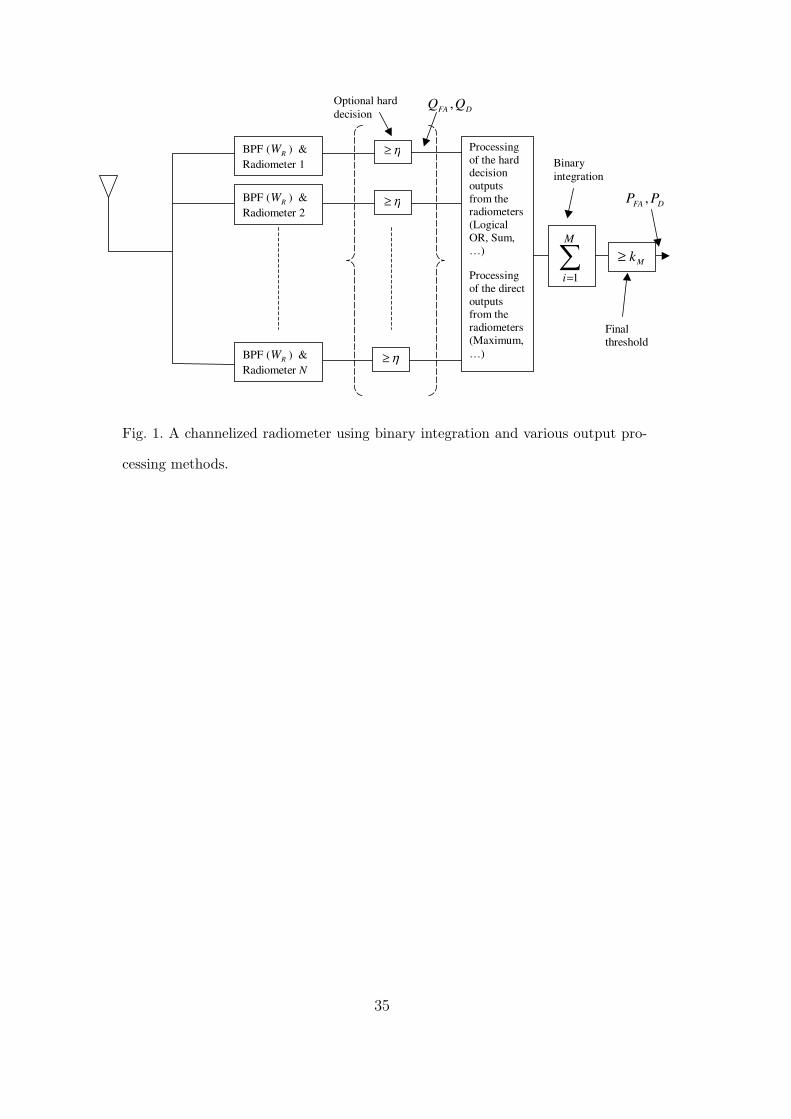
2.1 Basic Channelized Radiometer

Fig. 1 shows an intercept receiver that has N radiometers with adjacent fre-

quency ranges, which form the channelized radiometer, each with bandwidth

WR. The total bandwidth of the intercept receiver is NWR. The channelized

radiometer measures the received signal energy in adjacent channels with in-

tegration time TR. In the case of hard-decision processing, these energies are

compared to a threshold η. After hard-decision, the outputs from different

channels are combined with either a logical–OR [7],[8, p. 26],[18] operation

or a sum [12, 15]. The radiometer outputs from different channels can also

be directly combined by taking the largest output (maximum). Let M denote

the total number of observed time-intervals per decision. In all cases, the com-

bined outputs corresponding to different time-intervals are summed to form

the final decision variable W . The sum W is compared to a threshold kM . If

the sum is larger than or equal to the threshold it is decided that a signal was

present in addition to just noise, i.e., hypothesis H1 is accepted. Otherwise it

is decided that only noise was present in the received signal, i.e., hypothesis

H0 is selected. For simplicity, we assume synchronization with the hop timing

and that the frequency ranges of the individual radiometers match that of the

hop channels [14, 15]. Thus, TR = TH , M is the number of hops per decision,

and WR = WH . When the synchronization assumption is not valid there is

random splitting of the signal energy in time and/or frequency. This can be

approximately taken into account by adding energy loss to the required SNR

[8, p. 72-77]. According to Dillard [8], the effective energy loss resulting from

a random splitting of the signal energy in time into two cells of integration

is typically 0.5-2 dB. Asynchronous operation does not always result in SNR

11

loss: if the detection probability is limited by the intercept probability (no

matter how high SNR), asynchronous operation helps because it increases the

probability of intercept [18].

2.2 Sweeping Channelized Radiometer

Typically N < NH . In such a case, the detector can step the received fre-

quency band K times within each hop (synchronization is still assumed) to

increase the probability of intercept [15]. This means the integration time

per radiometer output is reduced, TR = TH/K. The radiometer outputs are

sampled before the center frequency is changed. This means that the total

number of radiometer outputs within a hop is Neff = KN . These outputs are

the measured energies. We index these outputs so that in the first phase the

outputs have indices 1, 2, . . . ,N ; in the second phase the outputs have indices

N +1, N +2, . . . , 2N , and so on. Due to the synchronization assumption, this

detection structure is analytically equivalent to Neff radiometers with band-

width WH and integration time TH/K [15]. Time–frequency product of each

individual radiometer is TRWR = (TH/K)WH . In the following, it is assumed

that TRWR is an integer or that it is rounded to an integer. Fig. 2 shows the

detection structure for the case of K = 3 detection phases per hop duration.

Sweeping makes the analytically equivalent instantaneous bandwidth large,

but the integration time is reduced. The probability of intercept per hop is

pI = Neff/NH ≤ 1, because all hop channels are assumed to be equally likely

(random frequency hopping). Note that in some systems it is possible to use

only a part of the channels. However, this is not considered here. In Fig. 2,

channels 1–12 are searched during one hop and there are 15 possible hop chan-

12

nels. Therefore, pI = 80%. The probability of intercept is the same if channels

2–13, 3–14 or 4–15 are searched instead. It is possible to combine sweeping

faster than hop dwell time and this ”hop level” sweeping (which does not af-

fect the results). For example, let us assume that NH = 16, N = 4 and K = 2.

Now channels 1–8 can be searched in the first hop and channels 9–16 in the

second hop (and 1–8 in the third hop and so on). If K = 1, the search pattern

could be 1–4, 5–8, 9–12, 13–16. If K = 4, all the channels are searched during

a single hop.

The energy of the frequency hopping signal in the time–frequency area of the

radiometer that intercepts the signal is assumed to be Eij = EH/K, where

EH is the received energy per hop, i is the hop index, i ∈ {1, 2, · · · , M},

and j is the radiometer output index, j ∈ {1, 2, · · · , Neff}. In practice, this

assumption is an approximation, and the signal may leak some energy also

to adjacent radiometers. Let Rij = 2Vij/N0, where Vij is the measured en-

ergy, denote the normalized (scaled with 2/N0) radiometer output. The local

decision Cij based on the (normalized) radiometer output is

Cij =

1, Rij > η

0, otherwise

The final decision variable is

W =M∑i=1

Wi, (1)

where Wi =Neff∑j=1

Cij assuming a sum is used to combine the local decisions.

A logical–OR operation can alternatively be used to combine all Neff local

decisions within a hop. In this case, the per hop decision variable Wi = 1 if at

13

least one Cij = 1, j ∈ {1, 2, · · · , Neff}; otherwise it is zero. The maximum–

based intercept receiver sums per hop maxima of the radiometer outputs [5,

11, 20], so that Wi = maxj {Rij}. In [5] the envelope detector outputs were

combined using the maximum and the performance was analyzed using the

normal approximation. Therein, the proposed detector was called the sum–of–

largest–envelopes (SLE) receiver. In [11] the channelized radiometer outputs

were combined with the maximum. Therein, numerical convolution and the

normal approximation were used. This can be viewed to be an extension of the

sum–of–largest–envelopes–squared (SLES) receiver [20] to a situation where

TRWR ≥ 1. In [20] it was found that the SLES receiver has slightly better

performance than the SLE receiver.

The statistical properties of the local decisions and the resulting decision rules

are analyzed in the next section. The optimal channelized radiometer output

combining method, based on the average-likelihood ratio, is considered in Sec-

tion 4.

3 Performance analysis

The statistical properties of the local decisions are discussed in Section 3.1.

Analysis of the logical OR–sum detector is presented in Section 3.2, followed

by the sum–sum detector analysis and the max–sum detector analysis in Sec-

tions 3.3 and 3.4, respectively. The analysis of the logical OR–sum detector in

Section 3.2 is based on [18]. It is presented to enable comparisons.

14

3.1 Instantaneous Radiometer Outputs

In the noise–only case, the distribution function of Rij can be approximated

by the chi-square distribution with 2TRWR degrees of freedom. In the deter-

ministic signal–and–noise case, the distribution can be approximated by the

non-central chi-square distribution with 2TRWR degrees of freedom and non-

centrality parameter λ = 2Eij/N0 [28]. The above results are usually called

exact although they are approximations in the case of the conventional analog

implementation [8].

The probability of false alarm is the probability that the radiometer output ex-

ceeds a threshold when only noise is present. The individual radiometers have

the probability of false alarmQFA = P (Rij > η|Eij = 0) = P (Cij = 1|Eij = 0).

It is given by [8, eq. 3.2]

QFA =

∞∫η

xTRWR−1e−x/2

2TRWRΓ (TRWR)dx, (2)

where η is the threshold and Γ is the gamma function [1, 6.1.1]. Based on (2)

we can calculate the threshold for the required probability of false alarm. The

probability of detection QD is the probability that the threshold is exceeded

when signal and noise are present, i.e., it is QD = P (Rij > η|Eij > 0) =

P (Cij = 1|Eij > 0). Assuming a deterministic signal [8, p. 57],[28]

QD = QTRWR

(√2Eij/N0,

√η), (3)

where QTRWR() is the generalized Marcum’s Q function [21, eq. (2-1-122)] with

parameter TRWR. The energy required for a given probability of detection QD

15

can be approximated with [18, Eq. (13a)]

Eij/N0 ≈ 1

2

([√η − (2TRWR − 1) /2 − Q−1 (QD)

]2

− (2TRWR − 1) /2

), (4)

where Q−1 is the inverse of the tail integral of the normal distribution. This

result with the exact threshold, i.e., inverse of the function (2), is a very

accurate approximation, especially when QD is relatively high.

3.2 Logical OR–Sum Decision Rule

The probability of false alarm per hop when using logical–OR is [18]

p0 = P (Wi = 1|H0) = 1 − (1 −QFA)Neff , (5)

because a false alarm occurs if at least one radiometer output exceeds the

threshold. The probability of detection per hop is [18]

p1 = P (Wi = 1|H1) =

pI

(1 − (1 −QD) (1 −QFA)Neff−1

)+ (1 − pI) p0,

(6)

because at most one time–frequency cell (radiometer output) can have signal

energy. The probability of this occurring is the probability of intercept, pI .

If the signal is not intercepted, the probability of detection is the false alarm

probability. The total probability theorem can be applied to combine these

two mutually exclusive events to get the result in (6). Assuming that the hop

positions are independent, the final probability of false alarm over M observed

16

hops is [7, 18]

PFA = P (W ≥ kM |H0) =M∑

i=kM

M

i

pi

0 (1 − p0)M−i, (7)

where kM is the final threshold that is used after summing the last M logical–

OR outputs. The final probability of detection is similarly [7, 18]

PD = P (W ≥ kM |H1) =M∑

i=kM

M

i

pi

1 (1 − p1)M−i. (8)

3.3 Sum–Sum Decision Rule

In [15], hard decision envelope detector has been studied. Therein, each lo-

cal decision is based on initial decisions which are based on magnitudes (en-

velopes) of the corresponding FFT outputs. These local decisions from all

channels and hops are summed and compared to a threshold, i.e., there are

three different thresholds. The detector performance was evaluated with the

normal approximation. In the sum–sum channelized radiometer considered

here the local decisions Cij are based on the radiometer outputs. There are

only two thresholds to be optimized. For the case studied in [15], a high proba-

bility of detection and a large number of hops, the normal approximation gives

reasonably good results. However, in most cases, the normal approximation is

not very accurate. In [12] exact results have been used. However, therein the

studied scenario was different and the probability of intercept (POI) was not

taken into account.

17

Here we will present an exact method to calculate the probability of detection

and false alarm for the sum–sum channelized radiometer. When only noise

is present, W follows the binomial distribution. Therefore, the probability of

false alarm is

PFA =MNeff∑i=kM

MNeff

i

Qi

FA (1 −QFA)MNeff−i . (9)

In the signal–and–noise case, the discrete density function of Wi is

fWi(x) = P (Wi = x|H1) = pIfWi

(x|H1,inter.) + (1 − pI) fWi(x|H0) , (10)

where fWi(x|H1,inter.) is convolution of a binomial density with parameters

Neff −1 and QFA and a binomial density with parameters 1 and QD. Function

fWi(x|H0) is a binomial density with parameters Neff and QFA. The density

function of the decision variable W is

fW (x) = fWi(x) ∗ fWi

(x) ∗ · · · ∗ fWi(x)︸ ︷︷ ︸

M

, (11)

which can be efficiently calculated with the FFT, and the final probability of

detection is found with

PD = 1 −kM−1∑x=0

fW (x). (12)

3.4 Max–sum Decision Rule

Because the conditional probability density functions in the signal–and–noise

case and the noise–only case are known [5, 11], we can calculate the corre-

18

sponding raw moments of the per hop decision variable Wi. Let Rk0 = E

{W k

i

}denote the kth raw moment in the noise–only case and Rk

1 = E{W k

i

}denote

the kth raw moment in the signal–and–noise case assuming interception. In

the noise–only case, the mean κ1, variance κ2 and third central moment κ3 of

the per hop maximum are

κ1 = R10

κ2 = R20 − (R1

0)2

κ3 = 2 (R10)

3 − 3R10R

20 + R3

0

The raw moments of the per hop maximum when taking the POI per hop

(pI) into account are Zk1 = pIR

k1 + (1 − pI)R

k0 . The mean, variance and third

central moment can be calculated in similar way as in the noise–only case.

Now, because the central moments of a sum of independent random variables

add up to the order of 3 we know the mean, variance and the third central

moment of decision variable W in both the noise–only case and the signal–

and–noise case. Instead of the traditional normal approximation that we used

in [11], we propose the use of more accurate shifted log–normal approximation

that is matched to the first three central moments of the sum [22]. The shifted

log–normal approximation is first used to obtain the threshold and then to

obtain the probability of detection. The shifted log–normal approximation is

especially useful when the number of observed hops is relative small. Fig.

3 shows comparison, corresponding to [11, Fig. 4], between the shifted log–

normal and normal approximations. It can be seen that the shifted log–normal

approximation is more accurate.

19

The method presented above requires knowledge of the raw moments of the

per hop maximum. In [11], the first two moments, to be used with the normal

approximation, were calculated with numerical integration. It is possible to

find the raw moments analytically by writing out the density function of the

maximum and performing symbolic integration using similar techniques as in

[5, 16]. As an example, in the special case TRWR = 1, the following simple

result is obtained

Rv0 = Neff2vΓ (v + 1)

×

Neff−1∑i=0

Neff − 1

i

(−1)Neff−1−i (Neff − i)−(v+1)

. (13)

However, this process is excessively tedious for practical values of the param-

eters (large TRWR and Neff ). Therefore, numerical integration will be used.

4 Optimal detection

4.1 Thresholded Outputs

A optimal detector conditioned on the observable C = {Cij}, i ∈ {1, 2, · · · , M},

j ∈ {1, 2, · · · , Neff}, i.e., the set of local decisions in all hops and channels,

has been derived in [15]. There it was derived in the context of the enve-

lope detector, but the result can also be directly applied in the case of the

channelized radiometer.

In [15], it was shown that at low signal-to-noise-ratios the sum–sum statistic is

20

asymptotically optimal. This does not mean that a detector based on the sum–

sum performs better than a detector based on the logical–OR. Actually, when

only one signal is present, the logical–OR based detector performs slightly

better.

4.2 Direct Outputs

The optimal detection statistic conditioned on the observable R = {Rij}, i.e.,

the set of normalized radiometer outputs, is [9]

Λ (R) =M∏i=1

1

NH

NH∑j=1

Λij (Ri| fj), (14)

where Ri denotes the set of normalized radiometer outputs in the hop i and

fj denotes the hypothesis that the signal is present in channel j. It is assumed

that the signal is equally likely to be in any channel and these channels are

independent from hop to hop. For the sweeping system, the likelihood ratio

Λij is 1 if Neff < j ≤ NH and if j ≤ Neff it is ([8, Eq. (A.12)])

Λij (Ri| fj) = c ·R−TRWR−1

2ij ITRWR−1

(√2EHRij

KN0

), (15)

where ITRWR−1 is the modified Bessel function of the first kind [1, 9.6] with

order TRWR − 1 and

c = 2TRWR−1

2

(EH

KN0

)−TRWR−1

2

Γ (TRWR) e− EH

KN0 . (16)

If no sweeping is used, i.e., K=1, and if also Neff = NH (14) and (15) form

the classical Woodring-Edell (WE) detector [14]. In this case, the constant

term can (16) can be ignored.

21

It can be observed that the optimal detection statistic depends on the signal-

to-noise ratio. The signal-to-noise ratio is usually unknown (it may be esti-

mated after detection) so the optimal detector is not realizable in practice.

However, it is important to study the optimal detector so that the upper

bound on detection performance is found. Note that because R contains more

information than C, the performance of a detector using the statistic (14) is

better than that of the optimal detector conditioned on thresholded radiome-

ter outputs C. The max–sum channelized radiometer also uses the observable

R. This allows it to have in most cases clearly better performance than the

logical–OR or sum–sum detectors. If details of the signal modulation would

be known (for example that the signal is a SFH/CPM signal) more specialized

optimal detection methods could be used [14]. It would be possible to evaluate

the performance of the optimal detector with approximations similar to those

used in [3, 4, 14]. However, in this paper we use simulations.

4.3 Calculating the likelihood ratio

For large values of TRWR, there exists an efficient representation of the Bessel

function, namely [1, 9.7.7]

Iv (z) =1√2πv

ev�(1 + (z/v)2

)1/4

{1 +

∞∑k=1

uk (t)

vk

}, (17)

where ( =(1 + (z/v)2

)1/2+ln (z/v)−ln

(1 +

√1 + (z/v)2

), t = 1

/√1 + (z/v)2

and u1 (t) = 1/8t− 5/24t3. For values of uk(t) with k > 1 refer to [1, 9.3.9].

22

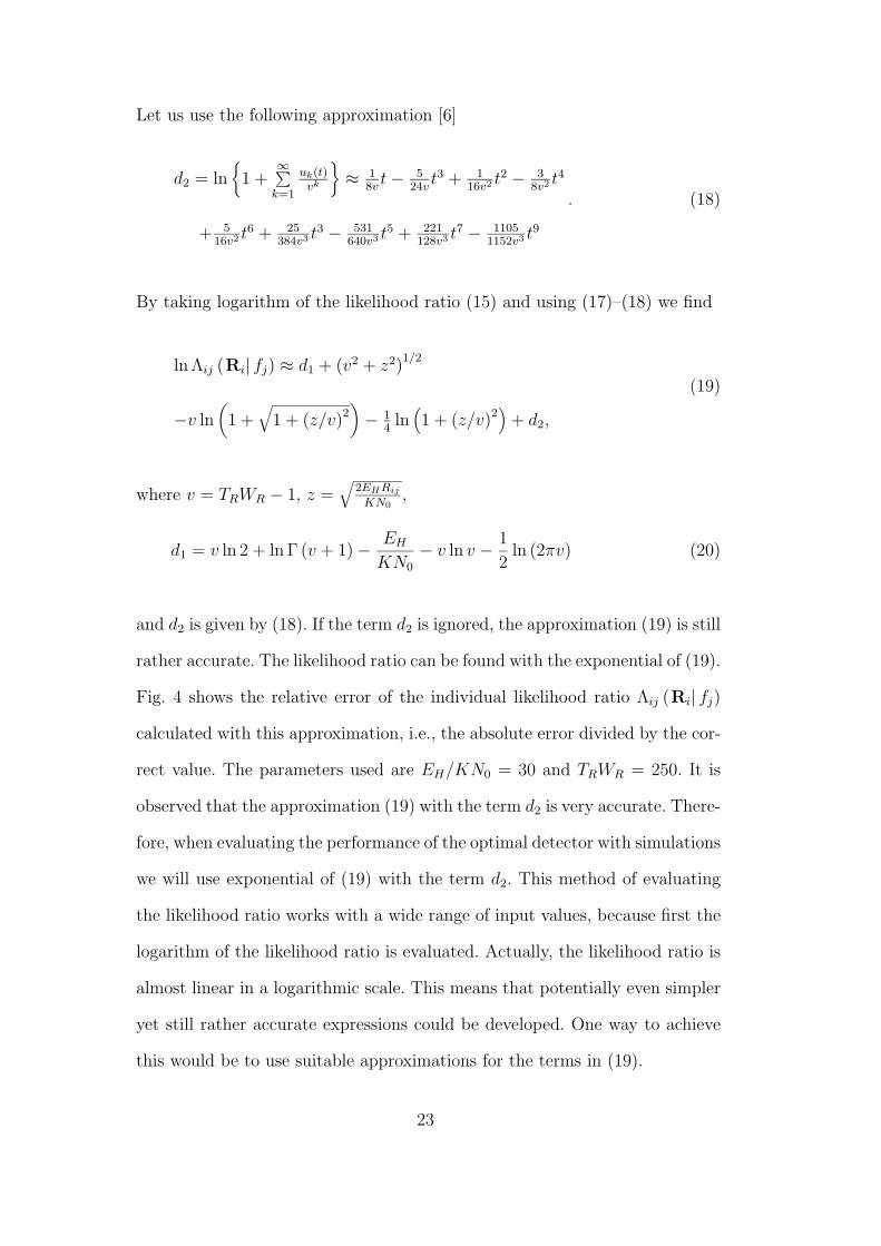
Let us use the following approximation [6]

d2 = ln{

1 +∞∑

k=1

uk(t)vk

}≈ 1

8vt− 5

24vt3 + 1

16v2 t2 − 3

8v2 t4

+ 516v2 t

6 + 25384v3 t

3 − 531640v3 t

5 + 221128v3 t

7 − 11051152v3 t

9

. (18)

By taking logarithm of the likelihood ratio (15) and using (17)–(18) we find

ln Λij (Ri| fj) ≈ d1 + (v2 + z2)1/2

−v ln(

1 +√

1 + (z/v)2)− 1

4ln(1 + (z/v)2

)+ d2,

(19)

where v = TRWR − 1, z =√

2EHRij

KN0,

d1 = v ln 2 + ln Γ (v + 1) − EH

KN0

− v ln v − 1

2ln (2πv) (20)

and d2 is given by (18). If the term d2 is ignored, the approximation (19) is still

rather accurate. The likelihood ratio can be found with the exponential of (19).

Fig. 4 shows the relative error of the individual likelihood ratio Λij (Ri| fj)

calculated with this approximation, i.e., the absolute error divided by the cor-

rect value. The parameters used are EH/KN0 = 30 and TRWR = 250. It is

observed that the approximation (19) with the term d2 is very accurate. There-

fore, when evaluating the performance of the optimal detector with simulations

we will use exponential of (19) with the term d2. This method of evaluating

the likelihood ratio works with a wide range of input values, because first the

logarithm of the likelihood ratio is evaluated. Actually, the likelihood ratio is

almost linear in a logarithmic scale. This means that potentially even simpler

yet still rather accurate expressions could be developed. One way to achieve

this would be to use suitable approximations for the terms in (19).

23

Numerical effects can also affect the calculation of the final decision variable

(14), which is a product of the sums of the individual likelihood ratios. It is

possible to take a logarithm of the final decision variable, which results in

a sum of logarithms of sums of the individual likelihood ratios. However, in

this case it is still necessary to sum exponentials (logarithm cannot be moved

inside a sum).

5 Performance Under Fading

We assume a frequency-nonselective (in the used hop channels) fading, con-

stant over each hop and independent from hop to hop. The frequency-nonselective

fading results in multiplicative distortion of the signal [21, p. 772-773]. Let us

denote the multiplicative scaling factor α. It is Rayleigh-distributed. The in-

stantaneous SNR is now γH = α2EH/N0(phase shift does not affect energy).

The instantaneous SNR (in each hop) is a random variable that follows the

chi-square distribution with two degrees of freedom [21, p. 773] with average

value γH , i.e., the density function is P (γH) = 1/γHe−γH/γH . The results are

given as a function of the average hop SNR, i.e, the average SNR is specified

and the instantaneous SNRs in each hop are independently fluctuating around

the the specified value.

Performance analysis of the logical OR–sum and the sum–sum based receivers

requires finding each individual radiometer’s probability of detection QD (as-

suming that signal is present in the time-frequency area of the radiometer).

The probability of detection for a fixed SNR is given by (3). The probability

24

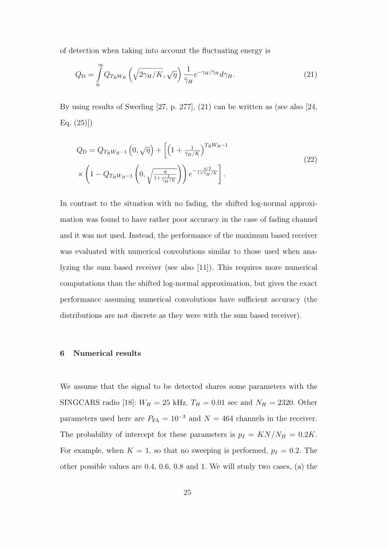
of detection when taking into account the fluctuating energy is

QD =

∞∫0

QTRWR

(√2γH/K,

√η)

1

γH

e−γH/γHdγH . (21)

By using results of Swerling [27, p. 277], (21) can be written as (see also [24,

Eq. (25)])

QD = QTRWR−1

(0,√η)

+[(

1 + 1γH/K

)TRWR−1

×(

1 −QTRWR−1

(0,√

η1+ 1

γH/K

))e− η/2

1+γH/K

].

(22)

In contrast to the situation with no fading, the shifted log-normal approxi-

mation was found to have rather poor accuracy in the case of fading channel

and it was not used. Instead, the performance of the maximum based receiver

was evaluated with numerical convolutions similar to those used when ana-

lyzing the sum based receiver (see also [11]). This requires more numerical

computations than the shifted log-normal approximation, but gives the exact

performance assuming numerical convolutions have sufficient accuracy (the

distributions are not discrete as they were with the sum based receiver).

6 Numerical results

We assume that the signal to be detected shares some parameters with the

SINGCARS radio [18]: WH = 25 kHz, TH = 0.01 sec and NH = 2320. Other

parameters used here are PFA = 10−3 and N = 464 channels in the receiver.

The probability of intercept for these parameters is pI = KN/NH = 0.2K.

For example, when K = 1, so that no sweeping is performed, pI = 0.2. The

other possible values are 0.4, 0.6, 0.8 and 1. We will study two cases, (a) the

25

number of hops observed per decision M = 300 and (b) M = 16.

The required energy for the sum–sum receiver, for a given threshold, was

calculated by first solving (9) for QFA as a function of kM and the desired false

alarm probability. Then the inverse of the chi-square cumulative distribution

function was used to find the threshold η for individual radiometers. Now QD

can be found by using (3) (no fading) or (22) (fading). The final probability of

detection was found with (12). The required SNR per cell corresponding to the

required probability of detection, for a given threshold kM , was found with a

search. Searching was also used to find the optimal threshold kM . The required

SNR for a logical OR–sum based channelized radiometer was calculated using

procedures similar to those in [18]. Optimal thresholds found with a search

were used. The required SNR for a maximum–based receiver was discovered

by using the shifted log–normal approximation (no fading) or with numerical

convolutions (fading). The optimal threshold of the maximum–based receiver

does not depend on SNR.

The required SNR for the optimal detector was found with simulation. Due

to a very large number of random variables to be generated, simulations in

the case (a) are excessively time consuming. Therefore, the performance of the

optimal detector was evaluated only in the case (b).

In the case (a) we additionally studied hard decision envelope detector pro-

posed in [15]. Its performance was evaluated via normal approximations similar

to those in [15]. We assumed that each envelope detector output containing

signal has equal signal component. In practice, the strength of signal compo-

nent varies and the results can be interpreted to be an approximation allowing

comparisons with other structures. Results we obtained were the same as those

26

in [15]. It would be possible to apply the exact results presented in this paper

for the sum–sum detector also for the envelope detector. Since we concentrate

on the channelized radiometer this was not pursued here further.

Fig. 5 shows the required energy per hop in the case (a) to achieve PD = 0.999

with the envelope detector [15], the sum–sum based channelized radiometer,

the logical OR–sum based channelized radiometer and the maximum based

channelized radiometer. It can be observed from Fig. 5 that the sum–sum re-

ceiver has practically the same performance as the logical OR–sum receiver.

It is anticipated that when multiple signals are present, the sum–sum based

receiver is better than the receiver using the logical OR–sum. Envelope detec-

tion is about 1 dB worse than the radiometer based solutions. When there is

no fading, the maximum based intercept receiver is the best of the receivers

discussed here, except when POI is 20%. When channel is fading, the logical

OR–sum and sum–sum receivers have better performance than the maximum

based intercept receiver. It is seen that when the number of hops observed is

large sweeping does not increase the probability of detection. It is more impor-

tant to have large detection SNR than to have large probability of intercept.

This is in line with the result in [15], obtained for the envelope detector based

system. When channel is fading the detection SNR is sometimes much higher

than the average value (it is a random variable). This explains why fading

actually improves performance. If the frequency band of the transmitter is

unknown, some type of frequency sweeping (at least in the hop level) should

be used. Otherwise the probability of intercept can be very low, even zero.

Fig. 6 shows the required energy per hop in the case (b) to achieve PD = 0.99

with the sum–sum based channelized radiometer, the logical OR–sum based

channelized radiometer, the maximum based channelized radiometer and the

27

optimum detector using detection statistic (14). It was not possible to get the

required PD without sweeping. This is because without sweeping, the prob-

ability that at least one radiometer intercepts the signal in any of the hops

is 1 − (1 − 0.2)16, which is 0.97185. Therefore, the maximum probability of

detection with any detector is 0.97185 · 1 + (1 − 0.97185) · 0.001, which is

smaller than 0.99. It is possible to get the required performance if K ≥ 2, i.e,

probability of intercept is greater than or equal to 40 %. It can be observed

from Fig. 6, that if the probability of intercept is greater than 40 % and there

is no fading, the maximum based detector is the best of the practical detec-

tors. When the probability of intercept is 100 %, the maximum based detector

has performance very close to that of the optimal detector. When channel is

fading, the logical OR–sum and sum–sum receivers have better performance

than the maximum based intercept receiver. It can be observed that also in

this case the sum–sum receiver and the logical OR–sum based receiver have

almost equal performance. In simulations, it was noticed that the thresholds

given by the shifted log–normal approximation are accurate. However, when

K = 2 there was a small difference between the required SNR given by simula-

tions and the approximation (0.08 dB). When K > 2 the difference was much

smaller (0.01–0.02 dB). This is because the shifted log–normal approximation

is not so good fit to the distribution of the decision variable when K = 2 as

when K > 2. In the case of fading, numerical convolutions were used instead

of the shifted log–normal approximation. In case (b) fading degrades perfor-

mance. This is because the number of intercepted hops can be small. When the

detection SNR is fading, quite often only a few of the intercepted hops have

”enough” detection SNR. When the number of intercepted hops increases, the

performance in the case of fading increases. The best performance in the case

of fading is achieved when K = 5 (POI is 100%).

28

The same methods can be used also with signals that have other parameters

(higher hop rate, larger bandwidth). Actually, the results depend only on

the time-bandwidth product, the number of channels in the signal and in

the receiver, the number of observed hops and the required PD and PFA per

decision. For example, if the hop rate is 10 000 hops/s and the bandwidth

of the channels is 2.5 MHz then the time-bandwidth product is 250. If the

other parameters do not change, the results are equal to those presented in

the paper.

7 Conclusions

The logical OR–sum channelized radiometer, the sum–sum channelized ra-

diometer, the max–sum channelized radiometer and the optimal detector us-

ing frequency sweeping have been analyzed. When sweeping is performed there

are multiple detection phases within each hop, i.e, sweeping is faster than the

hop dwell time. The numerical results presented here, for a slow frequency

hopping signal having parameters similar to those of the SINGCARS combat

radio, support the following conclusions. If the number of hops observed per

decision is large, frequency sweeping degrades the performance compared to

a system that does not apply frequency sweeping (with or without fading).

If the number of hops observed is small, sweeping is often necessary to get

the desired performance. When the channel is fading best performance is ob-

tained by using fast sweeping. Using a sum is only slightly worse than using

a logical–OR. If there is no fading, the maximum based intercept receiver has

the best performance of the practical receivers discussed here unless the prob-

ability of intercept (POI) is small. When POI is large, the performance of the

29

maximum based receiver is close to that of the optimal receiver. In the case of

fading, logical OR–sum and sum–sum receivers have better performance than

the maximum based receiver.

8 Acknowledgments

This work was supported by Finnish Defence Forces Technical Research Cen-

tre. The work of J. J. Lehtomaki was supported by Nokia Foundation and the

Graduate School in Electronics, Telecommunications and Automation, GETA.

The authors wish to thank the reviewers for their suggestions to improve the

manuscript. We also thank Ari Pouttu, Johanna Vartiainen, Harri Saarnisaari

and Keijo Ruotsalainen for their help with the article.

References

[1] M. Abramowitz and I. A. Stegun. Handbook of Mathematical Functions

with Formulas, Graphs, and Mathematical Table. National Bureau of

Standards, 1964.

[2] N. C. Beaulieu, W. L. Hopkins, and P. J. McLane. Interception of

frequency-hopped spread-spectrum signals. IEEE Journal on Selected

Areas in Communications, Vol. 8, No. 5, June 1990, pp. 853–870.

[3] U. Cheng, M. K. Simon, A. Polydoros, and B. K. Levitt. Statistical

models for evaluating the performance of coherent slow frequency-hopped

M-FSK intercept receivers. IEEE Trans. Commun., Vol. 42, No. 234,

February/March/April 1994, pp. 689–699.

[4] U. Cheng, M. K. Simon, A. Polydoros, and B. K. Levitt. Statistical

30

models for evaluating the performance of noncoherent slow frequency-

hopped M-FSK intercept receivers. IEEE Trans. Commun., Vol. 43, No.

234, February/March/April 1995, pp. 1703–1712.

[5] C. D. Chung. Generalised likehood-ratio detection of multiple-hop

frequency-hopping signals. IEE Proc.–Commun., Vol. 141, No. 2, April

1994, pp. 70–78.

[6] E. R. B. de Mello, V. B. Bezerra, and N. R. Khusnutdinov. Ground

state energy of massive scalar field inside a spherical region in the global

monopole background. Journal of Mathematical Physics, Vol. 42, No. 2,

February 2001, pp. 562–581.

[7] R. A. Dillard. Detectability of spread-spectrum signals. IEEE Trans.

Aerosp. Electron. Syst., Vol. 15, No. 4, July 1979, pp. 526–537.

[8] R. A. Dillard and G. M. Dillard. Detectability of Spread-Spectrum Signals.

Artech House, Norwood, Massachusetts, 1989.

[9] R. A. Dillard and G. M. Dillard. Likelihood-ratio detection of frequency-

hopped signals. IEEE Trans. Aerosp. Electron. Syst., Vol. 32, No. 2, April

1996, pp. 543–553.

[10] S. M. Kay. Fundamentals of Statistical Signal Processing: Detection The-

ory. Prentice Hall, Upper Saddle River, New Jersey, 1998.

[11] J. J. Lehtomaki. Maximum based detection of slow frequency hopping

signals. IEEE Commun. Lett., Vol. 7, No. 5, May 2003, pp. 201–203.

[12] J. J. Lehtomaki. Performance comparison of multichannel energy detec-

tor output processing methods. Proc. Seventh Int. Sympos. on Signal

Processing and Its Applications, Paris, France, July 2003, pp. 261–264.

[13] J. J. Lehtomaki, M. Juntti, and H. Saarnisaari. CFAR strategies for

channelized radiometer. IEEE Signal Processing Letters, Vol. 12, No. 1,

January 2005, pp. 13–16.

31

[14] B. K. Levitt, U. Cheng, A. Polydoros, and M. K. Simon. Optimum

detection of slow frequency-hopped signals. IEEE Trans. Commun., Vol.

42, No. 234, February/March/April 1994, pp. 1990–2000.

[15] B. K. Levitt, M. K. Simon, A. Polydoros, and U. Cheng. Partial-band de-

tection of frequency-hopped signals. Proc. IEEE Globecom’93, Houston,

USA, November/December 1993, pp. 70–76.

[16] C. H. Lim and H. S. Lee. Performance of order-statistics CFAR detector

with noncoherent integration in homogenous situations. IEE Proc. Radar

and Signal Processing, Vol. 140, No. 5, October 1993, pp. 291–296.

[17] S. J. MacMullan. The effect of multipath fading on the radiometric detec-

tion of frequency hopped signals. Proc. IEEE Third International Sympo-

sium on Spread Spectrum Techniques and Applications, Oulu, Finland,

July 1994, pp. 243–247.

[18] L. E. Miller, J. S. Lee, and D. J. Torrieri. Frequency-hopping signal

detection using partial band coverage. IEEE Trans. Aerosp. Electron.

Syst., Vol. 29, No. 2, April 1993, pp. 540–553.

[19] L. W. Nemsick and E. Geraniotis. Adaptive multichannel detection of

frequency-hopping signals. IEEE Transactions on Communications, Vol.

40, No. 9, September 1992, pp. 1502–1511.

[20] W. Ng and N. C. Beaulieu. Noncoherent interception receivers for fast

frequency-hopped spread spectrum signals. Proc. Canadian Conference

on Electrical and Computer Engineering’94, Halifax, Canada, September

1994, pp. 348–351.

[21] J. G. Proakis. Digital Communications, 3rd edition. McGraw-Hill, 1995.

[22] K. L. Q. Read. A lognormal approximation for the collector’s problem.

The American Statistician, Vol. 52, No. 2, May 1998, pp. 175–180.

[23] D. C. Schleher. Introduction to Electronic Warfare. Artech House, Nor-

32

wood, Massachusetts, 1986.

[24] D. A. Shnidman. Radar detection probabilities and their calculation.

IEEE Transaction on Aerospace and Electronic Systems, Vol. 31, No. 3,

July 1995, pp. 928–950.

[25] W. E. Snelling and E. Geraniotis. Sequential detection of unknown

frequency-hopped waveforms. IEEE Journal on Selected Areas in Com-

munications, Vol. 7, No. 4, May 1989, pp. 602–617.

[26] W. E. Snelling and E. Geraniotis. Analysis of compressive receivers for the

optimal interception of frequency-hopped waveforms. IEEE Transactions

on Communications, Vol. 42, No. 1, January 1994, pp. 127–138.

[27] P. Swerling. Probability of detection for fluctuating targets (originally

published in 1954 as RAND research memo RM-1217). IRE Transactions

on Information Theory, Vol. 6, No. 2, April 1960, pp. 269–308.

[28] H. Urkowitz. Energy detection of unknown deterministic signals. Pro-

ceedings of the IEEE, Vol. 55, No. 4, April 1967, pp. 523–531.

33

Figure captions:

Fig. 1 A channelized radiometer using binary integration and various output

processing methods.

Fig. 2 The detection structure in the synchronous case, 15 possible hop chan-

nels, 4 radiometers, 3 detection phases, signal intercepted in the first phase by

the radiometer 3, Neff = 12.

Fig. 3 Theoretical (normal and shifted log–normal approximations) and sim-

ulated miss probabilities for the maximum based channelized radiometer, 100

hops observed, 464 radiometers in the receiver, signal has 2320 FH-channels,

K=1 (POI 20%), PFA = 10−3 and the time–frequency product of the radiome-

ters TRWR = 250.

Fig. 4 Relative error of the approximation to the individual likelihood ra-

tio Λij (Ri| fj), EH/KN0 = 30, TRWR = 250 and j ≤ Neff .

Fig. 5 Required hop SNR, WH = 25 kHz, TH = 0.01, NH = 2320, M = 300,

PD = 0.999 and PFA = 10−3.

Fig. 6 Required hop SNR, WH = 25 kHz, TH = 0.01, NH = 2320, M = 16,

PD = 0.99 and PFA = 10−3.

34

Optional harddecision DFA QQ ,

Binaryintegration

BPF ( RW ) &Radiometer 1

η≥

η≥

η≥

Processingof the harddecisionoutputsfrom theradiometers(LogicalOR, Sum,…)

Processingof the directoutputsfrom theradiometers(Maximum,…)

�=

M

i 1

Mk≥

Finalthreshold

DFA PP ,BPF ( RW ) &Radiometer 2

BPF ( RW ) &Radiometer N

Fig. 1. A channelized radiometer using binary integration and various output pro-

cessing methods.

35

4=N

HT

KTH /

3=K

15=HN

Radiom. 4, Output 4

Radiom. 1, Output 1

Radiom. 4, Output 12

Radiom. 4, Output 8Radiom. 1, Output 9

Radiom. 1, Output 5

Radiom. 2, Output 2

Radiom. 3, Output 7Radiom. 2, Output 6

Radiom. 3, Output 11Radiom. 2, Output 10

Signal withenergy EH

Energy EH / K

Fig. 2. The detection structure in the synchronous case, 15 possible hop channels,

4 radiometers, 3 detection phases, signal intercepted in the first phase by the ra-

diometer 3, Neff = 12.

36

18 18.5 19 19.510

−4

10−3

10−2

10−1

100

SNR per hop [dB]

mis

s pr

obab

ility

Maximum based (simulated)Shifted log normal approximationNormal approximation

Fig. 3. Theoretical (normal and shifted log–normal approximations) and simulated

miss probabilities for the maximum based channelized radiometer, 100 hops ob-

served, 464 radiometers in the receiver, signal has 2320 FH-channels, K=1 (POI

20%), PFA = 10−3 and the time–frequency product of the radiometers TRWR = 250.

37

100 200 300 400 500 600 700 800 900 100010

−14

10−12

10−10

10−8

10−6

10−4

10−2

Rij

Rel

ativ

e er

ror

term d2 ignored

with term d2

Fig. 4. Relative error of the approximation to the individual likelihood ratio

Λij (Ri| fj), EH/KN0 = 30, TRWR = 250 and j ≤ Neff .

38

0.2 0.3 0.4 0.5 0.6 0.7 0.8 0.9 116

17

18

19

20

21

22

Probability of Intercept

Req

uire

d ho

p S

NR

[dB

]

Fading channel

No fading

Envelope detector based systemSum−sum channelized radiometerOR−sum channelized radiometerMax−sum channelized radiometer

Fig. 5. Required hop SNR, WH = 25 kHz, TH = 0.01, NH = 2320, M = 300,

PD = 0.999 and PFA = 10−3.

39

0.2 0.3 0.4 0.5 0.6 0.7 0.8 0.9 121

21.5

22

22.5

23

23.5

24

24.5

25

25.5

26

Probability of Intercept

Req

uire

d ho

p S

NR

[dB

]

Fading channel

No fading

Not possible to get the required performance

Sum−sum channelized radiometerOR−sum channelized radiometerMax−sum channelized radiometerOptimum detector

Fig. 6. Required hop SNR, WH = 25 kHz, TH = 0.01, NH = 2320, M = 16,

PD = 0.99 and PFA = 10−3.

40