Detection of Disease Gradually Changing Outbreaks Seasonal ...
113
Detection of Disease Outbreaks using State Space Models Master of Science Thesis Autumn 2011/Spring 2012 Tina Graungaard Department Department of Mathematical Sciences, Aalborg University Center for Cardiovascular Research, Aalborg Hospital, Aarhus University Hospital
Transcript of Detection of Disease Gradually Changing Outbreaks Seasonal ...

Detection of DiseaseOutbreaksusing State Space Models
Master of Science ThesisAutumn 2011/Spring 2012Tina Graungaard
Gradually ChangingSeasonal Variation ofCardiovascular Diseases- A Danish Nationwide Cohort Study
Master of Science ThesisSpring 2009Anette Luther Christensen
eDepartment of Mathematical Sciences, Aalborg UniversityCenter for Cardiovascular Research, Aalborg Hospital, AarhusUniversity Hospital
Department of Mathematical Sciences, Aalborg UniversityCenter for Cardiovascular Research, Aalborg Hospital,Aarhus University Hospital

Department of Mathematical Sciences, Aalborg UniversityCenter for Cardiovascular Research, Aalborg Hospital, AarhusUniversity Hospital
TITLE:Detection ofDiseaseOutbreaksusing State SpaceModels
SEMESTER:Master of Science ThesisNinth and tenth semester
PROJECT PERIOD:2/9/2011− 1/6/2012
WRITTEN BY:
Tina Graungaard
SUPERVISOR:P. Svante Eriksen
Number of copies: 6
Number of pages: 103
Finished: D. 1/6/2012
SYNOPSIS:Disease surveillance is the systematic collec-tion, analysis, interpretation and distributionof health data for preventing health relatedproblems. The primary purpose of diseasesurveillance is early detection of disease out-breaks for prevention of further morbidityand mortality. In Denmark disease surveil-lance is carried out by Statens Serum Insti-tut, which defines disease outbreaks as anunusual high number of incidences of a di-sease. The objective of this thesis is to com-pare different statistical models for prospec-tive detection of possible outbreaks. Adjust-ments for seasonal variations, secular trendsand past outbreaks should be incorporatedinto the model. Three different models areused: Farringtons algorithm, a dynamic lin-ear model and a multi-process dynamic lin-ear model. Comparison of the models is pre-sented applying data from Statens Serum In-stitut consisting of all samples tested positivefor Mycoplasma pneumoniae infections fromJuly 1994 to July 2005. The analysis indi-cate that the dynamic linear model and themulti-process dynamic linear model are supe-rior to Farringtons algorithm. The thresholdvalue in Farringtons algorithm is highly af-fected by the baseline values used in the cal-culations, where the dynamic linear modeland the multi-process dynamic linear modelare better at adapting to the seasonal varia-tions and past outbreaks. The multi-processdynamic linear model has the advantage thatit can identify outliers.


Preface
This master of science thesis is written by Tina Graungaard in the period fromSeptember 2011 to June 2012. The thesis is composed at the Department ofMathematical Sciences, Aalborg University, in cooperation with Center for Car-diovascular Research, Aalborg Hospital, Aarhus University Hospital. The au-thor would like to thank Center for Cardiovascular Research for making dataavailable and the statisticians for their inputs and comments.A basic knowledge equivalent to a bachelor degree in Mathematical Sciences atAalborg University is required.
Reading instructions
References throughout the report will be presented according to the numbermethod, and when a reference is placed before a period, it refers to the previousparagraph.Figures, tables, mathematical definitions, etc. are enumerated in reference tothe chapter i.e. the first figure in chapter 4 has number 4.1, the second hasnumber 4.2 etc.
The project is divided into two parts: Analysis and theory. In the first part theproblem of detection of disease outbreaks is outlined, and the analysis of thesamples tested positive for Mycoplasma pneumoniae using three different me-thods, Farringtons algorithm, the dynamic linear model and the multi-processdynamic linear model, is presented. The first part is completed by a discussionand a conclusion of the results. In the second part the basic theory for the threemethods is presented. First generalized linear models and in particular Poissonregression are presented. Then state space models and dynamic linear modelare introduced, and the part is finished with a presentation of the multi-processmodel.
I

II
Mathematical notation and symbols
Throughout the rapport the following mathematical notation and symbols areapplied.
R The set of all real numbersRn Real vector space of n-dimensional real vectorAT Transpose of a real matrix AA−1 Inverse of a real matrix Af(·), π(·) The density- or probability function of argumentsf(·|·), π(·|·) Conditional density function of argumentsf ′ The derivative of fN(µ, V ) Normal distribution with mean µ and variance VNp(µ,Σ) Multivariate normal distribution of dimension p with mean
vector µ and variance matrix ΣPo(µ) Poisson distribution with mean and variance µχ2(p) Chi square distribution with p degrees of freedom∼ Distributed asL(·) Likelihood function`(·) Log-likelihood functionU(·) Score statisticI The information matrixλ(·),W (·) The likelihood ratiori ResidualsD The devianceE[·] Expected valueVar[·] VarianceVar[·|·] Conditional varianceCov[·, ·] Covariance(Yt)t≥1 Time seriesy1:t y1, y2, . . . , ytYt Observation at time tθt State at time tvt Observation error at time twt Evolution error at time tFt Design matrix at time tGt Evolution matrix at time tVt Observation variance matrix at time tWt Evolution variance matrix at time tet Forecast erroret Standard innovationr The signal-to-noise ratio
Dansk resume
Overvagning af sygdomme involverer systematisk indsamling, dynamisk model-lering, analyse og fortolkning af sundhedsrelateret data for at forebygge og kon-trollere sygdomme, skader og andre sundhedsrelaterede problemer. Det primæreformal med overvagning af sygdomme er at detektere udbrud og epidemier tidligtfor at forebygge yderligere morbiditet og mortalitet. Overvagning af sygdommeudføres i Danmark af Statens Serum Institut, der definerer et udbrud som etunaturligt højt antal af inficerede af en bestemt sygdom.
Formalet med dette speciale er at sammenligne tre forskellige metoder til de-tektering af mulige udbrud. Metoder til automatisk detektering af mulige syg-domsudbrud skal tage højde for forskellige ting. Systematiske variationer somsæsonvariation og trend skal inkorporeres i modellen, og der skal tages højde fortidligere udbrud.
Den første metode blev præsenteret af Farrington et al. i 1996 og bruges afStatens Serum Institut til detektering af mulige sygdomsudbrud. Farringtonsalgoritme er baseret pa en log-lineær regressionsmodel, som justeres for over-spredning, sæsonvariation, trends og tidligere udbrud. En tærskelværdi udreg-nes baseret pa baseline værdier fra tidligere ar, og hvis det observerede antaler højere end denne tærskelværdi, markeres observationen som et muligt udbrud.
Den anden metode, der bruges, er en dynamisk lineær model, hvor det an-tages, at data er normalfordelt. Denne model bruger data fra tidligere ugertil at forudsige et interval en tidsenhed frem, hvor det forventes at næste ob-servation ligger indenfor. Hvis det observerede antal ligger over dette interval,markeres observationen som et muligt udbrud.
Den sidste metode er en multi-proces dynamisk lineær model, hvor det antages,at en enkelt dynamisk lineær model ikke kan beskrive data. I stedet for brugestre dynamisk lineære modeller til at beskrive tre forskellige tilstande, som detantages, at data kan være i. De tre tilstande er stabil tilstand, hvor der ikke erudbrud, outlier, hvor en observation afviger uden der er udbrud og den tredje
III

IV
mulighed er muligt sygdomsudbrud. Der bruges en første ordens Markov struk-tur til at beskrive overgangen mellem de tre forskellige modeller.
De tre metoder sammenlignes ved at analysere data fra Statens Serum Institut,som bestar af alle prøver, som er testet positiv for Mycoplasma pneumoniaeinfektioner fra juli 1994 til juli 2005. I denne periode er der to udbrud, somer identificeret af Statens Serum Institut. Analysen viser, at Farringtons al-goritme pavirkes meget af hvilke baseline værdier, som bruges til udregning aftærskelværdien. Hvis baseline værdier falder sammen med tidligere udbrud, af-spejles dette i tærskelværdien, og hvis der kun haves en begrænset mængde data,bliver sæsonvariation detekteret som mulige udbrud. Dette giver stor usikkerhedi, hvornar et muligt sygdomsudbrud detekteres. Den dynamiske lineære modelog den multi-proces dynamisk lineære model er derimod bedre til at tilpasse sigsæsonvariationen og bliver ikke pavirket af tidligere udbrud. Begge modellergiver færre falsk positive alarmer end Farringtons algoritme. Det ser ud til, atden dynamiske lineære model detekterer udbruddene før multi-proces dynamisklineære modellen. Multi-proces dynamiske lineære modellen har den fordel, atposterior sandsynligheder for de tre mulige tilstande fas, og derfor er muligt atidentificere outliers.

Contents
1 Introduction 1
I Analysis: Detection of Disease Outbreaks 7
2 Materials and Methods 92.1 Mycoplasma pneumoniae . . . . . . . . . . . . . . . . . . . . . . 92.2 Data preprocessing . . . . . . . . . . . . . . . . . . . . . . . . . . 92.3 Farringtons algorithm . . . . . . . . . . . . . . . . . . . . . . . . 13
2.3.1 Model structure . . . . . . . . . . . . . . . . . . . . . . . 142.4 The dynamic linear model . . . . . . . . . . . . . . . . . . . . . . 182.5 The multi-process dynamic linear model . . . . . . . . . . . . . . 19
3 Results 21
4 Discussion 29
5 Conclusion 35
II Theory 37
6 Generalized linear models 396.1 Exponential family . . . . . . . . . . . . . . . . . . . . . . . . . . 39
6.1.1 Expected value and variance of a(Y ) . . . . . . . . . . . . 396.1.2 The score statistic and the information . . . . . . . . . . 41
6.2 Generalized linear models . . . . . . . . . . . . . . . . . . . . . . 426.3 Maximum likelihood estimation . . . . . . . . . . . . . . . . . . . 436.4 Inference . . . . . . . . . . . . . . . . . . . . . . . . . . . . . . . . 45
6.4.1 Confidence interval . . . . . . . . . . . . . . . . . . . . . . 486.5 Poisson distribution . . . . . . . . . . . . . . . . . . . . . . . . . 496.6 Poisson regression . . . . . . . . . . . . . . . . . . . . . . . . . . 50
V

VI Contents
7 State space models 537.1 Dynamic linear models . . . . . . . . . . . . . . . . . . . . . . . . 547.2 State estimation and forecasting . . . . . . . . . . . . . . . . . . 55
7.2.1 Filtering . . . . . . . . . . . . . . . . . . . . . . . . . . . . 557.2.2 Kalman filter for DLM . . . . . . . . . . . . . . . . . . . . 577.2.3 Smoothing . . . . . . . . . . . . . . . . . . . . . . . . . . 597.2.4 Forecasting . . . . . . . . . . . . . . . . . . . . . . . . . . 62
7.3 The innovation process and model checking . . . . . . . . . . . . 657.4 Model specification . . . . . . . . . . . . . . . . . . . . . . . . . . 66
7.4.1 Trend models . . . . . . . . . . . . . . . . . . . . . . . . . 677.4.2 Linear growth model . . . . . . . . . . . . . . . . . . . . . 707.4.3 Seasonal models . . . . . . . . . . . . . . . . . . . . . . . 70
7.5 Estimation of unknown parameters . . . . . . . . . . . . . . . . . 73
8 Multi-process models 758.1 Multi-process model class I . . . . . . . . . . . . . . . . . . . . . 768.2 Multi-process model class II . . . . . . . . . . . . . . . . . . . . . 78
8.2.1 First-order Markov . . . . . . . . . . . . . . . . . . . . . . 80
Bibliography 91
A Codes 93A.1 Data preprocessing . . . . . . . . . . . . . . . . . . . . . . . . . . 93A.2 Farringtons algorithm . . . . . . . . . . . . . . . . . . . . . . . . 95A.3 The dynamic linear model . . . . . . . . . . . . . . . . . . . . . . 97A.4 The multi-process dynamic linear model . . . . . . . . . . . . . . 99

Chapter 1
Introduction
Disease surveillance is the systematic collection, analysis, interpretation and dis-tribution of health data for preventing and controlling disease, injury and otherhealth related problems. In public health services disease surveillance has se-veral purposes, where the primary purpose is the detection of disease outbreaksand epidemics. Early detection is important, because more effective disease in-tervention can prevent further morbidity and mortality [1]. Interventions couldbe removal of contaminated food, vaccination or preventively treating indivi-duals at risk [2]. Disease surveillance can also give information about the natu-ral development of diseases, for example how long the incubation period is, or itcan be used to determine the size and range of an outbreak or epidemic. Finallydisease surveillance can be used for evaluating and monitoring how interventionsaffect the public health [1],[3].
Ongoing advice and communication
Identification of a problem e.g. an outbreak
Advice and guidance
Intervention
Effect
Surveillance
Figure 1.1: Illustration of surveillance system [3].
1

2 1. Introduction
Figure 1.1 illustrates a surveillance system consisting of several components,that are part of a cycle. During the surveillance, data is collected and registered,then the data is analysed, and possible problems are identified, for example anoutbreak. Afterwards, if necessary, interventions can be made, and new datacan be collected for analysis to study the effects of the interventions. Not alldiseases are under surveillance, only diseases of serious character, and diseasesthat can be prevented e.g. through vaccinations [3].
In disease surveillance one critical problem is the definition of an outbreak. TheCenters for Disease Control and Prevention, which carry out disease surveil-lance throughout the United States, define an outbreak as two or more casesof infection, that are epidemiologically connected. This definition can be usefulin retrospective analysis, when detailed epidemiological information is available,but in prospective analysis this definition is of little help [2]. In Denmark thesurveillance is carried out by Statens Serum Institut under the Danish Ministryof Health [4]. Statens Serum Institut defines disease outbreaks as an unusualhigh number of incidences of a specific disease [5]. This definition, however,can be used for prospective detection of outbreaks, where the aim is to detectunusual high number of incidences as they occur. Thus an outbreak is first iden-tified, when the number of reported infected is higher than an expected level.When the number of reported infected exceeds the expected level, it is calledan aberration. Further epidemiological investigations have to be carried out todetermine if it is an actual outbreak, or it is clusters caused by the reportingsystem [2].
In prospective analysis the data must be analysed, as it is collected, and itis therefore not possible to accurately account for potential reporting delays asin retrospective analysis, where complete data often are available. Because it isdifficult to determine the exact time of infection, the date of report is often usedas a reference date. Alternatively the delay can be estimated and incorporatedinto the model, thereby introducing additional uncertainty. Thus it is importantto reduce the variability of the reporting delay for example by standardizing theprocedure for identification of infected individuals throughout the area undersurveillance. Another problem in prospective analysis is validation of data be-cause of the importance of early intervention for prevention of further morbidityor mortality. Therefore the uncertainty is higher in prospective analysis. Theneed for early interventions is also further complicated by the reporting delay [2].
During the last century the development in public health surveillance has beenmonumental, and the demand from diseases under surveillance exceeds the ca-pabilities for manual scanning [1],[6]. Therefore a computer-aided detectionsystem for detection of potential outbreaks is desired [6].
3
A computer-aided detection system has to fulfill several requirements for it to bereliable. One requirement is that the detection system has high sensitivity and alow false detection rate, where the sensitivity is given by the proportion of trueoutbreaks detected by the system, and the false detection rate is the proportionof false positives i.e. the proportion of observations marked as abnormal butnot associated with outbreaks. If the detection system had low sensitivity ora high number of false positive the confidence in the system would be compro-mised. Reporting delays also affect the detection sensitivity and specificity ofthe system as well as the timeliness [2].
A robust algorithm is needed to handle a wide variety of organisms with differingepidemiologies and frequencies. In other words it must be capable of handlingrare organisms with low frequency counts, and common organisms with highfrequency count [2].
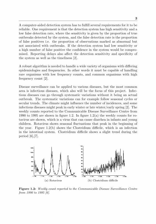
Disease surveillance can be applied to various diseases, but the most commonarea is infectious diseases, which also will be the focus of this project. Infec-tious diseases can go through systematic variations without it being an actualoutbreak. The systematic variations can for example follow seasonal cycles orsecular trends. The climate might influence the number of incidences, and someinfectious diseases might peak in early winter or late winter/early spring [2]. Theweekly counts reported to the Communicable Disease Surveillance Centre from1990 to 1995 are shown in figure 1.2. In figure 1.2(a) the weekly counts for ro-tavirus are shown, which is a virus that can cause diarrhea in infants and youngchildren. Rotavirus shows seasonal fluctuations that peak in the beginning ofthe year. Figure 1.2(b) shows the Clostridium difficile, which is an infectionin the intestinal system. Clostridium difficile shows a slight trend during theperiod [6],[7].
550 FARRINGTON, ANDREWS, BEALE AND CATCHPOLE [Part 3,
100. 1200.
90
1000. 80,
70. 800. 80
6001 50 1
400 30.)
20 200
10
:_____________________________________________________________ 0W0 1 1.90 1.1 91 1. 1. 92 1.1 93 1.1 94 1.1.95 1.1.90 1.1.91 1. 1.92 1.1.93 1.1.94 1.1.95
(a) (b) 7
700. 6
600. 5
500. 4
400.
3 300.
2 200
1 100.
0 0 _ _ _ _ _ _ _ _ _ _ _ _ _ 1 1.90 1.1.91 1.1.92 1 1,93 1.1 94 1 1 95 1.1.90 1.1'.91 1.1.92 1.1.93 1. 1.94 1.1.95
(c) (d)
240.
140.
200. 120.
160 100.
120 90.
80 80.
40.
40 20.
0 _ _ _ _ _ _ _ _ _ _ _ _ _ _0 1 1,90 1.1 91 1 192 1 193 1.1 94 1 1.95 1 1.90 1. 1.91 1,1.92 1,1'.93 1.1'.94 1.1'.95
Fig. 1. Weekly count of selected organisms reported to the CDSC, 1990-95: (a) rotavirus; (b) Clostridium difficile; (c) Salmonella derby; (d) Shigella sonnei; (e) influenza B; (f) Salmonella typhimurium DT104
2.3. Requirements of Routine Scanning System The main requirements of a routine scanning system are timeliness, sensitivity and
specificity, together with readily interpretable outputs. Timeliness and sensitivity are required to ensure that outbreaks are detected in time for interventions to take place, but this should not be at the cost of a disproportionately high false positive detection rate, which would result in wasted time and effort, and undermine confidence in the system.
These requirements to a large extent determine the statistical features of the system. In practice the week's data must be processed automatically, typically over a
(a) Rotavirus
550 FARRINGTON, ANDREWS, BEALE AND CATCHPOLE [Part 3,
100. 1200.
90
1000. 80,
70. 800. 80
6001 50 1
400 30.)
20 200
10
:_____________________________________________________________ 0W0 1 1.90 1.1 91 1. 1. 92 1.1 93 1.1 94 1.1.95 1.1.90 1.1.91 1. 1.92 1.1.93 1.1.94 1.1.95
(a) (b) 7
700. 6
600. 5
500. 4
400.
3 300.
2 200
1 100.
0 0 _ _ _ _ _ _ _ _ _ _ _ _ _ 1 1.90 1.1.91 1.1.92 1 1,93 1.1 94 1 1 95 1.1.90 1.1'.91 1.1.92 1.1.93 1. 1.94 1.1.95
(c) (d)
240.
140.
200. 120.
160 100.
120 90.
80 80.
40.
40 20.
0 _ _ _ _ _ _ _ _ _ _ _ _ _ _0 1 1,90 1.1 91 1 192 1 193 1.1 94 1 1.95 1 1.90 1. 1.91 1,1.92 1,1'.93 1.1'.94 1.1'.95
Fig. 1. Weekly count of selected organisms reported to the CDSC, 1990-95: (a) rotavirus; (b) Clostridium difficile; (c) Salmonella derby; (d) Shigella sonnei; (e) influenza B; (f) Salmonella typhimurium DT104
2.3. Requirements of Routine Scanning System The main requirements of a routine scanning system are timeliness, sensitivity and
specificity, together with readily interpretable outputs. Timeliness and sensitivity are required to ensure that outbreaks are detected in time for interventions to take place, but this should not be at the cost of a disproportionately high false positive detection rate, which would result in wasted time and effort, and undermine confidence in the system.
These requirements to a large extent determine the statistical features of the system. In practice the week's data must be processed automatically, typically over a
(b) Clostridium difficile
Figure 1.2: Weekly count reported to the Communicable Disease Surveillance Centrefrom 1990 to 1995 [6].

4 1. Introduction
Systematic variations should be incorporated into the system when calculatingbaselines and thresholds to reduce the false detection rate. Past aberrations oroutbreaks also needs to be included in the model to reduce the false detectionrate. The easiest way to do this is by omitting the data corresponding to pastaberrations or outbreaks from baselines and thresholds calculations. Alterna-tively a weight function can be used, where data relating to past aberrations oroutbreaks are down-weighted [2].
In 1996 Farrington et al. presented an algorithm for early detection of out-breaks of infectious diseases based on a log-linear regression model. The modelaccounts for overdispersion, seasonality, trends and past outbreaks. Historicaldata is used to calculate a threshold value, and if the observed count is abovethis threshold it is declared an aberration [6]. Farringtons algorithm is a widelyused algorithm for detection of disease outbreaks, and is currently being used byStatens Serum Institut in Denmark to monitor the gastrointestinal pathogensSalmonella, Campylobacter, Yersinia enterocolitica, Shigella and E. coli [8],[9].In England and Wales Farringtons algorithm is used by the Health ProtectionAgency to detect outbreaks in laboratory-based surveillance data [10].
In 2006 Cowling et al. compared three different methods for monitoring in-fluenza surveillance data. The focus was to find a valid and reliable way todetect the onset of a peak season, which did not require more than 9 weeks ofbaseline data. The first method was a dynamic linear model, which is a specialcase of a state space models. This model uses the previous information to cal-culate a forecast interval, and if the observed count falls outside this interval,then the count is identified as an aberration. The second method is a regressionmodel, where a forecast interval is calculated based on the normal distributionfrom the preceding weeks. The third method is a cumulative sum method,CUSUM, where the prediction error from the past d weeks is summed up, andif it exceeds a predefined threshold, it is defined an aberration. The comparisonis made using data from Hong Kong and the United States, where the dynamiclinear model was superior to the other models in the data from Hong Kong, andin the data from the United States the dynamic linear model and the CUSUMmethod performed similarly but better than the regression model. Thus thedynamic linear model is the preferred method of the three [11].
In 1983 Smith et al. used a multi-process dynamic linear model for monitoringrenal transplants. The interest was in developing an on-line statistical proce-dure for monitoring the kidney function of patients who had received kidneytransplants, specially changes that indicated rejection of the transplant. Theyassumed that the system could be in different states: Steady state, changes inthe system or outlier [12]. Similarly to the model presented by Smith et al.Whittaker et al. presented a dynamic change-point model for detecting the

5
onset of growth in bacteriological infections. They used an on-line decision pro-cedure to determine whether bacteriological infections were present in feedstuff[13].
Aim of the thesis
The aim of this thesis is to compare different methods for detection of outbreaks.The first method is the algorithm presented by Farrington et al. and is currentlybeing used by Statens Serum Institut for detection of aberrations [6],[8]. Thesecond method is a dynamic linear model equivalent to that presented by Cow-ling et al. [11]. The last method is a multi-process dynamic linear model, whichis similar to the model presented by Smith et al. and the change-point modelby Whittaker et al. for detection of abrupt changes in patterns [12],[13].
The comparison is presented applying data from Statens Serum Institut in Den-mark consisting of all samples tested positive for Mycoplasma pneumoniae in-fections from July 1994 to July 2005.Mycoplasma pneumoniae is the cause of a broad spectrum of respiratory infec-tions. Incidences occur all year but is most frequent in the fall and the winter.In Denmark outbreaks occur every four to six years, where they typically beginslowly during the late summer and have a duration of 3 to 4 months. My-coplasma pneumoniae is diagnosed by detection of Mycoplasma pneumoniaeDNA in respiratory secretion. It is not possible to prevent Mycoplasma pneu-moniae infections, but they can be limited by treatment and isolation of infectedindividuals [14].


Part I
Analysis: Detection ofDisease Outbreaks
7

Chapter 2
Materials and Methods
In this chapter the materials and methods of analysis are described. First thedata preprocessing is presented, then the method described by Farrington et al.,Farringtons algorithm, which is currently being used by Statens Serum Institut,is introduced [6],[8]. Furthermore a dynamic linear model and a multi-processdynamic linear model are presented.
2.1 Mycoplasma pneumoniae
Mycoplasma pneumoniae is a microorganism that causes of a broad spectrumof respiratory infections e.g. pneumonia, bronchitis and infections in the upperrespiratory system. The transmission of the microorganism occur in areas withmany people, and the incubation time is about 2 to 3 weeks. The symptoms aredry cough, fever, headache, sore throat, rash and ear complications. No effectivevaccine exist, but the duration of the disease can be shortened by treatment e.g.antibiotics [15]. Mycoplasma pneumoniae infections occur all year, but is mostcommon in the fall and early winter. Epidemics occur every 4 to 6 years andthe extent varies with average about 3 to 4 months [14].There were two outbreaks of Mycoplasma pneumoniae in the period Juli 1st1994 to Juli 29th 2005. The first outbreak was in 1998/1999, and the secondoutbreak was in 2004/2005 [16],[17].
2.2 Data preprocessing
The data was received as a csv file containing 4047 observations obtained dailyfrom Juli 1st 1994 to Juli 29th 2005. Each observation consist of the observation
9
10 2. Materials and Methods
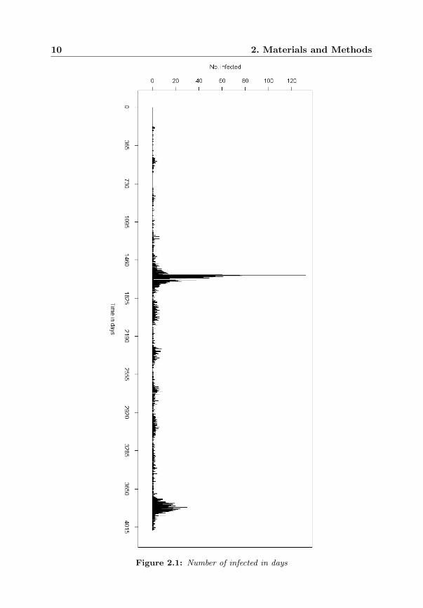
Figure 2.1: Number of infected in days
2.2 Data preprocessing 11
number, the date, and the number of samples tested positive for Mycoplasmapneumoniae the current day. The data analysis using Farringtons algorithm waspreformed using R 2.10.0 and the R-package surveillance [18], which includesFarringtons algorithm. The analysis using the dynamic linear model and themulti-process dynamic linear model were carried out using R 2.15.0 and theR-package dlm [19].
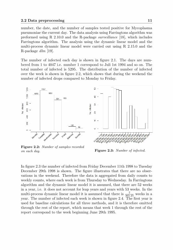
The number of infected each day is shown in figure 2.1. The days are num-bered from 1 to 4047 i.e. number 1 correspond to Juli 1st 1994 and so on. Thetotal number of infected is 5295. The distribution of the number of infectedover the week is shown in figure 2.2, which shows that during the weekend thenumber of infected drops compared to Monday to Friday.
Figure 2.2: Number of samples recordedon each day. Figure 2.3: Number of infected.
In figure 2.3 the number of infected from Friday December 11th 1998 to TuesdayDecember 29th 1998 is shown. The figure illustrates that there are no obser-vations in the weekend. Therefore the data is aggregated from daily counts toweekly counts, where each week is from Thursday to Wednesday. In Farringtonsalgorithm and the dynamic linear model it is assumed, that there are 52 weeksin a year, i.e. it does not account for leap years and years with 53 weeks. In themulti-process dynamic linear model it is assumed that there is 7
365.25 weeks in ayear. The number of infected each week is shown in figure 2.4. The first year isused for baseline calculations for all three methods, and it is therefore omittedthrough the rest of the report, which means that week 1 through the rest of thereport correspond to the week beginning June 29th 1995.

12 2. Materials and Methods
Figure 2.4: Number of infected in weeks

2.3 Farringtons algorithm 13
Figure 2.5 is a frequency plot of the observations, which shown that the distri-bution is skewed. Four observations, where the number of observed is higherthan 140, are omitted from the figure. The weeks omitted are week 230 to 233,where the number of infected is 383, 246, 246, and 235, respectively.
Figure 2.5: Frequency of observations
2.3 Farringtons algorithm
In this section the first method for analysis is presented. The described methodis a generalized linear model or more specifically a log-linear regression modelpresented by Farrington el al. in 1996 [6].
Farringtons algorithm is an algorithm for epidemiological surveillance and wasdeveloped to assist in early detection of outbreaks of infectious diseases [6]. Thisalgorithm is being used by Statens Serum Institut in Denmark for monitoring ofthe gastrointestinal pathogens pathogens Salmonella, Campylobacter, Yersiniaenterocolitica, Shigella, and E. coli [8]. Farringtons algorithm is also being usedby the Health Protection Agency in England and Wales to detect outbreaks inlaboratory-based surveillance data [10].
The primary purpose is to detect outbreaks early enough to have time for in-tervention. The algorithm must take seasonal cycles, secular trends and pastoutbreaks into consideration, and it must be sufficiently robust to handle a widerange of different diseases. Data collected for surveillance systems are often sub-ject to bias and delays in reporting. This makes the use of such data problematicfor early detection of outbreaks [6].
Seasonal variations affect many diseases, and the number of affected individualsmay peak at different times of the year or show long-term trends. The primaryinterest of the surveillance system is to detect increases greater than the seasonal

14 2. Materials and Methods
variability and the trends. Some variation is not of primary interest such asabnormally low counts, or if the count is unusual high but does not constitutean outbreak [6].
A routine scanning system has to fulfill different requirements such as timeliness,sensitivity, specificity, and the output has to be easy to interpret. The statisticalfeatures of the system is determined by these requirements, and one algorithmthat can analyse all diseases is developed [6].
2.3.1 Model structure
A flexible algorithm that takes seasonal patterns, underlying trends and noisein the data into account is designed. This is done by developing a log-linearregression model which is adjusted for overdispersion, seasonality, secular trendand past outbreaks. The model is used to calculate a threshold value, where itis expected that the next observed count is below. If the observed count for thenext observation is above the threshold value, the count is considered unusual[6].
There will occur delays between the time of infection and when it is reportedbecause it takes time to diagnose diseases. Since it is difficult to determine theexact time of infection the date of report is used as reference date. Trends aretaken into account in the model by fitting a linear time variable in the regressionmodel, and seasonality is considered by calculating the threshold value basedon comparable baseline periods from previous years [6].
Baseline
The baseline periods in weeks are calculated by letting b be the number of yearsback in time and w be half of the width of a chosen window. The present weekis denoted x of year y, and data for weeks x−w to x+w of years from y− b toy − 1 is used, which gives n = b(2w + 1) baseline weeks. The value of n affectthe precision, the need for a high n value for high precision, must be consideredin relation to the width of the window and the seasonal variations [6].
Regression model
Let yi denote the baseline count connected to baseline week ti, which is assumedto be distributed with mean µi and variance φµi, and the baseline values areassumed to be independent of each other. If the frequency of the disease is lowthe assumption of independence between the baseline counts is expected, butfor diseases of high frequency correlation between baseline counts are expected.Farrington et al. examined the correlation between baseline values for organisms
2.3 Farringtons algorithm 15
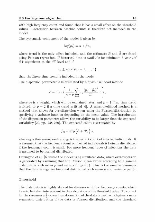
with high frequency count and found that is has a small effect on the thresholdvalues. Correlation between baseline counts is therefore not included in themodel.
The systematic component of the model is given by
log(µi) = α+ βti,
where trend is the only effect included, and the estimates α and β are fittedusing Poisson regression. If historical data is available for minimum 3 years, ifβ is significant at the 5% level and if
µ0 ≤ max{yi|i = 1, . . . , n},
then the linear time trend is included in the model.
The dispersion parameter φ is estimated by a quasi-likelihood method
φ = max
{1
n− pn∑
i=1
ωi(yi − µi)2
µi, 1
},
where ωi is a weight, which will be explained later, and p = 1 if no time trendis fitted, or p = 2 if a time trend is fitted [6]. A quasi-likelihood method is amethod that allows for overdispersion when using the Poisson distribution byspecifying a variance function depending on the mean value. The introductionof the dispersion parameter allows the variability to be larger than the expectedvariability [20, pp. 258-260]. The expected count is estimated by
µ0 = exp(α+ βt0
)s,
where t0 is the current week and y0 is the current count of infected individuals. Itis assumed that the frequency count of infected individuals is Poisson distributedif the frequency count is small. For more frequent types of infections the datais assumed to be normal distributed.
Farrington et al. [6] tested the model using simulated data, where overdispersionis generated by assuming that the Poisson mean varies according to a gammadistribution with mean µ and variance µ(φ− 1). This is the same as assumingthat the data is negative binomial distributed with mean µ and variance φµ [6].
Threshold
The distribution is highly skewed for diseases with low frequency counts, whichhave to be taken into account in the calculation of the threshold value. To correctfor the skewness a 2
3 -power transformation of the data is used, which gives a moresymmetric distribution if the data is Poisson distribution, and the threshold

16 2. Materials and Methods
become more accurate. High frequency data remains almost unaffected by thetransformation.
Given that the data is Poisson distributed and using the delta method, then
f(y0) = y2/30
can be approximated by
f(y0) ≈ f(µ0) + f ′(µ0)(y0 − µ0),
and the mean value of f(y0) is given by
E[y2/30
]= µ
2/30 .
The variance of f(y0) is
Var[y2/30
]= f ′(µ0)2Var [y0]
=
(2
3µ−1/30
)2
· φµ0
=4
9φµ
1/30 ,
and
Var[µ2/30
]=
4
9µ−2/30 Var[µ0],
where Var[µ0] is given as the variance of the fitted Poisson regression. On the23 -power scale the prediction error variance is given by
Var[y2/30 − µ2/3
0
]=
4
9τµ
1/30 ,
where
τ = φ+Var[µ0]
µ0.
Then an approximate 100(1− 2α)% prediction interval (L,U) for y0 is definedas
U = µ0
{1 +
2
3zα
(τ
µ0
)1/2}3/2
,
L = µ0 max
{1− 2
3zα
(τ
µ0
)1/2}3/2
, 0
,
where zα is the 100(1−α)-percentile of the normal distribution. If the frequencycount of infected individuals is outside this interval it is considered as unusual,and if it is above the threshold U it is considered a possible outbreak [6].

2.3 Farringtons algorithm 17
Past outbreaks
When calculating the baseline count, the calculations are based on historicaldata. If there has been an outbreak in the historical data used, this must beconsidered in the model. If past outbreaks are included in the calculations, thenthe threshold will be to high and the sensitivity will be reduced. Past outbreaksare included in the model by using a reweighting procedure that reduces theinfluence of high baseline counts. Residuals are given by
si
(φ)
=3
2φ1/2
y2/3i − µ2/3
i
µ1/6i (1− hii)1/2
where hii are the elements on the diagonal of the hat matrix. The hat matrix isa matrix that maps the vector of observed values into the vector of fitted values.If the data is Poisson distributed, where φ = 1, the residuals are known as thestandardised Anscombe residuals. The weights are given by
ωi =
{γsi(1)−2 if si > 1,
γ otherwise ,
i.e. corresponding to φ = 1, and where γ is a constant which satisfy∑ωi = n.
Empirical data is used to give low weights to counts with large residuals. Thereweighting reduces the effect of past outbreaks, but it does not eliminate it [6].
The algorithm
When a new observation is available, the following algorithm is applied to thevector of counts. First an initial model is fitted, and the initial estimated µi andφ are calculated. Then the weights are calculated and the model is fitted oncemore. The dispersion parameter φ is estimated again, and the model is rescaled.The trend is left out if it is not significant and the procedure is repeated. Thethreshold value is computed using historical data.
The analysis is carried out with the following parameters. For baseline cal-culations the number of years back in time used are b = 5, if available, and halfof the chosen window is w = 3, which gives maximum n = 35 baseline weeks.The data did not show a significant trend, which was therefore omitted. A 2
3 -power transformation was used for threshold calculations, and a weight functionwas used to reduce the influence of past outbreaks. To reduce the number ofsporadic cases detected as possible outbreaks for organisms with low frequencycounts, the restriction that the number of infected within the last 4 weeks hasto exceed 5 for an alarm to occur, is implemented [6].
18 2. Materials and Methods
2.4 The dynamic linear model
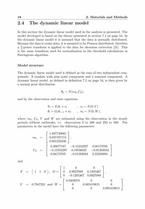
In this section the dynamic linear model used in the analysis is presented. Themodel developed is based on the theory presented in section 7.1 on page 54. Inthe dynamic linear model it is assumed that the data is normally distributed.Because the data is count data, it is assumed to be Poisson distributed, thereforea 2
3 -power transform is applied to the data for skewness correction [21]. Thisis the same transform used for normalization in the threshold calculations inFarringtons algorithm.
Model structure
The dynamic linear model used is defined as the sum of two independent com-ponents: A random walk plus noise component and a seasonal component. Adynamic linear model, as defined in definition 7.2 on page 54, is then given bya normal prior distribution
θ0 ∼ N(m0, C0),
and by the observation and state equations
Yt = Ftθt + vt , vt ∼ N(0, V )
θt = Gtθt−1 + wt , wt ∼ N(0,W ),
where m0, C0, V and W are estimated using the observation in the steadyperiods without outbreaks, i.e. observation 0 to 200 and 250 to 500. Theparameters in the model have the following parameters
m0 =
1.8877490850.0217071740.001223346
,
C0 =
0.30877187 −0.15352297 0.08173705−0.15352297 0.19556025 −0.012830340.08173705 −0.01283034 0.23292694
and
F =[
1 1 0], G =
1 0 00 0.9927089 0.12053670 −0.1205367 0.9927089
,
V = 0.7947231 and W =
0.0403078 0 00 0.005419615 00 0 0.005419615
.

2.5 The multi-process dynamic linear model 19
A significant level of α = 0.01 was used, and if an observation was above the 99%prediction interval when running the Kalman filter, then an alarm was given.If an observation was above the 99% prediction interval it was changed to NAin the data, and the Kalman filter was run again. The standard innovationsis analysed to determine whether the observations in the steady periods arenormally distributed for checking of the model assumptions.
2.5 The multi-process dynamic linear model
In this section the multi-process dynamic linear model used for analysis is pre-sented. The model developed is based on the theory presented in section 8.2 onpage 78. As for the dynamic linear model a 2
3 -power transform of the observationis used for skewness correction.
Model structure
A multi-process model class II is used for the analyses, where the probabilitieswith which the model is selected are first-order Markov. Three different modelstates are defined:
1. Steady state
2. Outlier
3. Possible outbreak
The three different states are modeled using a dynamic linear model, and themodels are defined as the sum of two independent components: A random walkplus noise component and a seasonal component. The matrices Ft and G arefor all three models given as
G = I3 and Ft =[
1 cos(2π 7365.25 · t) sin(2π 7
365.25 · t)].
The steady state model is defined as model 1 with variance parameters
V = 0.7947231 and W =
0.0403078 0 00 0.005419615 00 0 0.005419615
,
which is the same parameters as in the dynamic linear model described in thelast section.

20 2. Materials and Methods
The outlier model is defined as model 2, and it is assumed that the obser-vation variance is 10 times the observation variance of the steady state model,but the state variance is the same. Thus the variance parameters are
V = 7.947231 and W =
0.0403078 0 00 0.005419615 00 0 0.005419615
.
The model for possible outbreaks is defined as model 3. The variance param-eters are the same as for the outlier model, but the two models differ in thetransition probabilities, which are defined as
SteadyOutlierOutbreak
Steady Outlier Outbreak
0.985
0.010
0.005
0.985
0.010
0.005
0.090
0.010
0.900
1
.The transition probabilities should be read as there is a 98.5% probability ofstaying in steady state if the previous model was steady state. If the previousstate was outbreak, then there is a 9% probability that the new state is steady.The transition probabilities are chosen so 98.5% of the time series is in steadystate.
For each time t the filtering distribution is approximated using the multi-processKalman filter, proposition 8.2 presented on page 82, but instead of using mixturecollapses the aim is to retain the most probable model sequences. The numberof possible model sequences at time k is 3k. Suppose that at time t ≥ k thereare stored 3k model sequences. Then for t + 1 the likelihood for all 3k+1 pos-sible model sequences are calculated, and the 3k model sequences with highestlikelihood are saved, i.e. if k = 4 then 81 model sequences are saved. So at agiven time t ≥ k there are the model sequences
Mj = (α1j , . . . , αtj)
and their likelihoods Lj for j = 1, . . . , 3k. Let
Im = {j|αtj = m} , m = 1, 2, 3,
then the posterior probability of model m at time t is approximated by
Pr(αt = m) =
∑j∈Im Lj∑Lj
.
The most likely model sequences are selected at each time, because of the largenumber of mixture components as time progress, which increases the complexityof the calculations, thus the components where the posterior probabilities aresmall are ignored.
Chapter 3
Results
In this chapter the results of the analysis using the three different methods arepresented. Statens Serum Institut has identified two outbreaks of Mycoplasmapneumoniae in the period Juli 1st 1994 to Juli 29th 2005, the first in 1998/1999and the second in 2004/2005 [16],[17]. The years 1998/1999 correspond to theweek 132 to 208, and the years 2004/2005 correspond to the week 445 to 525,i.e. it is expected to detect an outbreak in each of these time periods. It isassumed, that there are no outbreaks in the weeks outside these periods, i.e.there are no outbreaks in week 1 to 131 and week 209 to 444. If there is analarm in the periods with no outbreak, it is considered a false positive alarm.
Farringtons algorithm
In figure 3.2 the results of the analysis using Farringtons algorithm are presented,where the number of infected, the threshold and alarms are shown. In the firstyears there are a number of alarms indicating a possible outbreak without therebeing a high number of infected. As time passes more data become availablefor baseline values, thereby increasing the amount of data used for thresholdcalculations. The threshold is affected by the first outbreak up to 5 years after,even though a weight function is used to reduce the effect of past outbreaks bygiving low weights to counts with high residuals. The threshold values duringthe second outbreak are not affected by the first outbreak, because the thresholdis only calculated using historical data up to 5 years back.
Dynamic linear model
Figure 3.3 shows the result of the analysis using the dynamic linear model, in-dicating the number of infected, the threshold and the alarms. There are no
21

22 3. Results
alarms in the first two years and only one false alarm before the period, wherethe first outbreak is expected. The threshold values are not affect by past out-breaks, and it easily adapt to the seasonal variations.
The dynamic linear model rely on the assumption that the observations arenormally distributed. This can be examined by checking that the standard in-novations in the steady periods are normally distributed. Figure 3.1 is a QQ-plotof the standard innovations in the steady periods, where it is shown, that thestandard innovations deviate slightly from the normal distribution, which couldindicate systematic deviation. This is, however, disregarded, and it is assumedthat the standard innovations are normally distributed.
Figure 3.1: QQ-plot of the standard innovations in the steady periods.
Multi-process dynamic linear model
In figure 3.4 the results of the analysis using a multi-process dynamic linearmodel are presented. The most likely sequence of models is shown, where thenumber of infected, outliers and the alarms are indicated. This shows that thereare two clusters of alarms corresponding to the two periods where outbreaksare expected. Two outliers are identified, where the first outlier in week 152correspond to an unusual high number of infected that week, and the second inweek 339 is an unusual low number of infected that week.

23
Figure 3.2: Result of analysis using Farringtons algorithm.

24 3. Results
Figure 3.3: Result of analysis using the dynamic linear model.

25
Figure 3.4: Results of analysis using multi-process dynamic linear model.

26 3. Results
Comparison
Table 3.1 shows week 145 to 178 along with the number of infected, the thres-hold values and the alarms using Farringtons algorithm and the dynamic linearmodel, DLM, and the weeks with alarms using the multi-process dynamic linearmodel, MDLM. These weeks correspond to part of the years 1998/1999, wherethe first alarms are indicated by the three methods. Farringtons algorithm givesthe first alarm in week 148, but the number of infected is only 3 this week, andit therefore questionable whether this is the beginning of the outbreak. Thesame argument applies to the alarms indicated by Farringtons algorithm in thefollowing weeks, even thought the number of infected become more frequent. Inweek 176 the number of infected is 38, but in the following week 177 the numberis 129, which is well above the threshold values given by Farringtons algorithm.
The first alarm given by the dynamic linear model is in week number 152,but there are no alarms in the next 12 weeks, i.e. the next alarm is in week 165.This could indicate that the alarm in week 152 is a false positive, but furtherepidemiological investigations need to be carried out to determine this. Thereare no alarms in the three weeks following week 165, and it is not until week171, that there are alarms in each week until the number of infected decreasesagain. The threshold values for the dynamic linear model are higher than thethreshold for Farringtons algorithm.
The multi-process dynamic linear model gives the first alarm in week 174, andthere are alarms from this week to week 200 except week 186.
WeekNo. Farringtons algorithm DLM MDLM
infected Threshold Alarm Threshold Alarm Alarm145 2 2.180402 No 6.379180 No No146 1 1.443721 No 6.596930 No No147 1 1.443721 No 6.364031 No No148 3 1.443721 Yes 6.206510 No No149 1 1.443721 No 6.888621 No No150 3 1.443721 Yes 6.658264 No No151 3 1.915426 Yes 7.298282 No No152 13 2.321480 Yes 7.832231 Yes No153 2 2.321480 No 8.100284 No No154 4 2.268024 Yes 8.071196 No No155 2 2.038544 No 8.897144 No No156 6 2.154036 Yes 8.729422 No No157 4 2.249601 Yes 10.067662 No No158 5 2.294297 Yes 10.450053 No No

27
159 8 1.952740 Yes 11.097567 No No160 6 2.087300 Yes 12.561153 No No161 12 2.466892 Yes 13.078961 No No162 14 2.905565 Yes 15.290707 No No163 11 2.905565 Yes 17.625298 No No164 9 2.905565 Yes 18.576575 No No165 21 2.871391 Yes 18.627691 Yes No166 14 2.871391 Yes 19.233855 No No167 12 2.887439 Yes 20.711052 No No168 12 2.887439 Yes 21.022993 No No169 24 2.742993 Yes 21.189470 Yes No170 13 3.520094 Yes 21.608446 No No171 25 4.202538 Yes 21.790446 Yes No172 30 4.924282 Yes 22.074671 Yes No173 31 5.715024 Yes 22.292990 Yes No174 47 7.056105 Yes 22.443546 Yes Yes175 44 8.247032 Yes 22.525668 Yes Yes176 38 8.382453 Yes 22.539931 Yes Yes177 129 8.883971 Yes 22.488170 Yes Yes178 383 8.858443 Yes 22.373464 Yes Yes
Table 3.1: Results of analysis using the three different methods. Weeks, the numberof infected, the threshold and alarms for weeks 145 to 178 are shown.
In table 3.2 week 478 to 492 are shown and again the number of infected, thethreshold values and the alarms for Farringtons algorithm and the dynamic lin-ear model, and the alarms for the multi-process dynamic linear model are given.These weeks corresponds to part of the years 2004/2005, which are equivalentto the weeks where the second outbreak is expected. The first alarm given byFarringtons algorithm is in week 484, and except for week 486 there is an alarmseach week until the number of infected decreases again.
The dynamic linear model gives the first alarm in the period, where the sec-ond outbreak is expected, in week 481, and there are alarms each week untilthe number of infected decreases again. The threshold values for the dynamiclinear model are lower than the threshold values for Farringtons algorithm.
For the multi-process dynamic linear model alarms occur from week 484 to513.
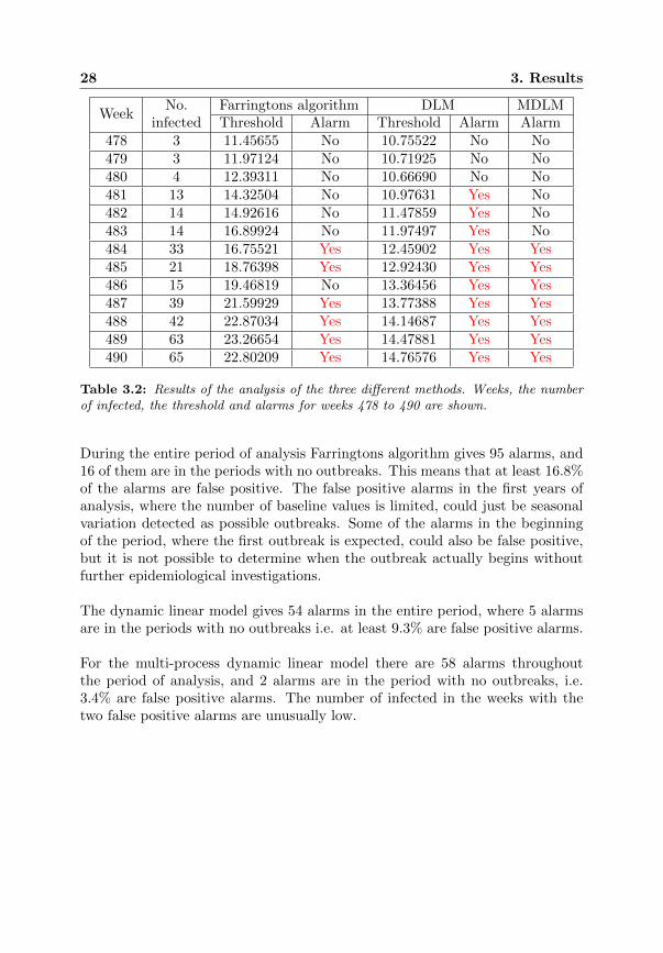
28 3. Results
WeekNo. Farringtons algorithm DLM MDLM
infected Threshold Alarm Threshold Alarm Alarm478 3 11.45655 No 10.75522 No No479 3 11.97124 No 10.71925 No No480 4 12.39311 No 10.66690 No No481 13 14.32504 No 10.97631 Yes No482 14 14.92616 No 11.47859 Yes No483 14 16.89924 No 11.97497 Yes No484 33 16.75521 Yes 12.45902 Yes Yes485 21 18.76398 Yes 12.92430 Yes Yes486 15 19.46819 No 13.36456 Yes Yes487 39 21.59929 Yes 13.77388 Yes Yes488 42 22.87034 Yes 14.14687 Yes Yes489 63 23.26654 Yes 14.47881 Yes Yes490 65 22.80209 Yes 14.76576 Yes Yes
Table 3.2: Results of the analysis of the three different methods. Weeks, the numberof infected, the threshold and alarms for weeks 478 to 490 are shown.
During the entire period of analysis Farringtons algorithm gives 95 alarms, and16 of them are in the periods with no outbreaks. This means that at least 16.8%of the alarms are false positive. The false positive alarms in the first years ofanalysis, where the number of baseline values is limited, could just be seasonalvariation detected as possible outbreaks. Some of the alarms in the beginningof the period, where the first outbreak is expected, could also be false positive,but it is not possible to determine when the outbreak actually begins withoutfurther epidemiological investigations.
The dynamic linear model gives 54 alarms in the entire period, where 5 alarmsare in the periods with no outbreaks i.e. at least 9.3% are false positive alarms.
For the multi-process dynamic linear model there are 58 alarms throughoutthe period of analysis, and 2 alarms are in the period with no outbreaks, i.e.3.4% are false positive alarms. The number of infected in the weeks with thetwo false positive alarms are unusually low.

Chapter 4
Discussion
In this project different methods for detection of outbreaks were compared byanalysing weekly counts of Mycoplasma pneumoniae. The different methodspresented in this project are intended as an aid to automatic detection of out-breaks, because the demands from diseases under surveillance exceeds the ca-pabilities for manual scanning. The three methods are Farringtons algorithm,the dynamic linear model and the multi-process dynamic linear model. For eachmethod the weeks with alarms were presented, and the number of alarms thatare clearly false positive were given. The weeks, where an outbreak was expectedto occur, were further investigated to evaluate the possible onset of the outbreak.
The data analysed in this project was collected by Statens Serum Institut, whichcarries out surveillance in Denmark [8]. In the analyses it is assumed that thedata is collected from the same region and that the diagnoses are validated.However, if these assumptions are not true it should be taken into account informulation of the models. It is also assumed that there are no variation in thereporting delay throughout the period of analysis. The date of report is usedas reference date thereby ignoring the reporting delay. Another approach couldhave been to apply a correction factor to the data based on an estimate of thedelay distribution. This, however, requires the date of infection, which are notavailable. The disadvantage of estimating the reporting delay is that additionaluncertainty is introduced into the system. The timeliness of the system is af-fected by the mean of the reporting delay, because the longer the delay is, thelonger it takes for an outbreak to be detected. The sensitivity of the detectionsystem is affected by the variance of the reporting delay, since the variabilityreduces the change that a threshold will be exceeded [2].
In this project data is aggregated from days into weeks to reduce the varia-bility throughout the week. This also reduces the number of observations with
29

30 4. Discussion
no infected and small counts. An alternative approach, if analysis on daily ba-sis is desired, could be to use a weight function that account for weekends andholidays.
There is not adjusted for an increase in the population throughout the periodeither, and the influence of the change in population size has not been furtheranalysed, but an increase would also affect the results. There was an increaseof about 214000 people in the population size in the period January 1st 1994 toJanuary 1st 2005 [22].
The distribution of the data is assumed to be Poisson, because it is count data.Farringtons algorithm accommodate this assumption by using a log-linear re-gression model, but a 2
3 -power transformation for normalization is used in thethreshold calculation, which is based on a normal prediction interval. The dy-namic linear model and the multi-process dynamic linear model rely on the as-sumption that the data is normally distributed. To achieve normally distributeddata a 2
3 -power transformation is used for skewness correction. To validate theassumption that the data is normally distributed the standard innovations dur-ing the steady period have to be normally distributed. The QQ-plot of the stand-ard innovations shows that the standard innovations deviate from the normaldistribution and the assumption of normality may not be meet. Alternatively ageneralized dynamic linear model or a multi-process generalized dynamic linearmodel could be used. These types of models allows the observations and thestate process to follow other distributions than the normal distribution e.g. thePoisson distribution.
The threshold value in Farringtons algorithm is highly affected by the base-line values used in the calculations. When a small amount of data is availablefor baseline values, Farringtons algorithm is likely to detect seasonal variationsas possible outbreaks resulting in false positive alarms. Past outbreaks also havean effect on the threshold value even though a reweighting procedure is used togive low weights to counts with high residuals. Both Farringtons algorithm andthe dynamic linear model are based on a forecast interval when defining thethreshold, but where Farringtons algorithm is highly affected by the baselineused, the dynamic linear model is better at adapting to the underlying expectedseasonal variation.
The parameters in the dynamic linear model and the multi-process dynamiclinear model are estimated based on the steady period of the time series. Thisintroduces bias, because the time series under analysis is also used for estimationof the unknown parameters. Ideally the parameters should be estimated basedon a period not under analysis. The threshold defined in Farringtons algorithmis only based on the previous history of the time series.

31
The dynamic linear model and the multi-process dynamic linear model are de-fined as consisting of two components: a random walk plus noise and a seasonalcomponent, where the seasonal component is defined as having a period of 52week. There was not included a trend in Farringtons algorithm, because it wasnot significant. Therefore a trend component was not used when formulatingthe dynamic linear model and the multi-process dynamic linear model.
For both Farringtons algorithm and the dynamic linear model it is assumedthat there are 52 weeks in a year i.e. 364 day. In Farringtons algorithm this isused to identify the corresponding baseline weeks previous years for thresholdcalculations, and in the dynamic linear model it is used in definition of the sea-sonal component. Thus the assumption of 52 weeks in a year shift the baselinevalues and the estimated seasonal variation, since there are 365 days in a yearand leap years is not taken into account. In the multi-process dynamic linearmodel, however, it is assumed that there are 365.25 days in a year, therebyaccounting for the 365 days in a year and leap years.
A 99% prediction interval is used to define the threshold for Farringtons al-gorithm and the dynamic linear model. The size of the prediction interval waschosen to reduce the number of false positives, but the size of the interval alsoaffect how early an outbreak is detected. A smaller prediction interval couldmean that outbreaks are detected earlier, but it could also give more false po-sitive alarms.
It is not possible to define the precise onset of the outbreaks, and which modelis the first to detect the two outbreaks, but the alarms still gives an indicationof when the outbreaks are detected by the three methods. For the first outbreakFarringtons algorithm indicates an outbreak before the dynamic linear modeland the multi-process dynamic linear model. The number of infected in thefirst weeks, where Farringtons algorithm gives alarms, is on the other hand low,and it is therefore questionable when the outbreak is detected at early. Thepossible false positive alarms in the first years of analysis could be caused bythe limited baseline values available for threshold calculations. In the periodwhere the first outbreak is expected, the dynamic linear model has few sporadicalarms in the week 160 to 170, but it is not until week 171, that there is alarmeach week until the number of incidences decreases again. The multi-processdynamic linear indicate an outlier in the beginning of the period, where the firstoutbreak is expected, and indicate that the onset of the outbreak is week 174 i.e.three weeks after the dynamic linear model. The second outbreak is indicatedby Farringtons algorithm to begin in week 484, but then there is a week withoutalarm in week 486. The first alarm given by the dynamic linear model is threeweeks before Farringtons algorithm in week 481, and the multi-process dynamiclinear model indicates an outbreak from week 484.
32 4. Discussion
Farringtons algorithm gave 16 identified false positive alarms, and the dynamiclinear model indicated 5 false positive alarms. The multi-process dynamic lin-ear model gave 2 false positive alarms in the steady period between the twoidentified outbreaks, but these alarms were in weeks, where the number of in-fected was unusually low. The number of false positive is considerable higherfor Farringtons algorithm than the dynamic linear model and the multi-processdynamic linear model. The multi-process dynamic linear model is defined so itdetect observations, where the variance of the state process is high, as outliersor outbreaks. This is why both unusual high counts or unusual low counts isdetected as possible outliers or outbreaks.
The multi-process dynamic linear models has the advantages over both Farring-tons algorithm and the dynamic linear model that it can differentiate betweenseveral possible models; in this case steady state, outlier and outbreaks. Thismeans that it is possible to detect outliers separately, whereas both Farringtonsalgorithm and the dynamic linear model only distinguish between no outbreakand possible outbreak. The results reflect this, where week 152 is marked as apossible outbreak by Farringtons algorithm and the dynamic linear model, butis identified as an outlier by the multi-process dynamic linear model.
In the multi-process dynamic linear model the different models are selectedat each time with known probability. The dependence structure of the modelsis first-order Markov, i.e. the model at each time t only depend on the model attime t− 1. It is, however, possible that the model at time t depends on modelsprior to time t − 1. This dependence structure could be achieved by using ahigher-order Markov structure of the models. The transition probabilities are aqualified guess based on the assumption that 98.5% of the time the time seriesis in steady state. The probabilities should, however, be analysed further, sincean outbreak of Mycoplasma pneumoniae occur every 4 to 6 years with a dura-tion of 3 to 4 months according to Statens Serum Institut, which correspond tomore than 1.5% of the time. It is also assumed that the transition probabilitiesare fixed throughout the year, but the time of the year, where outbreaks occur,could depend on the seasonal variation. Thus an outbreak could be more likelyto occur in a period, if there is a higher number of infected because of seasonalvariation.
The complexity of the calculations of the multi-process dynamic linear model isreduced by ignoring possible model sequences with low posterior probability. Itis, however, possible that sequences with low posterior probability in the begin-ning, which is ignored, later could be relevant.
33
The comparisons of Farringtons algorithm, the dynamic linear model and themulti-process dynamic linear model are only performed by analysing the numberof samples tested positive for Mycoplasma pneumoniae. One of the requirementsof the detection system is that it should be able to handle a wide variety oforganisms with varying organism count. Mycoplasma pneumoniae is one ofthe more common microorganisms, the methods should also be compared usingother data with lower and higher organism count than Mycoplasma pneumoniae.


Chapter 5
Conclusion
The aim of this project was to compare different methods for detection of di-sease outbreaks. The three different methods were Farringtons algorithm, thedynamic linear model and the multi-process dynamic linear model. Farringtonsalgorithm is currently being used by Statens Serum Institut.
Analysis of Mycoplasma pneumoniae using the three different methods indicatesthat the dynamic linear model and the multi-process dynamic linear model aresuperior to the log-linear regression model presented by Farrington et al. Far-ringtons algorithm is highly affected by the baseline values used for thresholdcalculations, where the dynamic linear model and the multi-process dynamiclinear model are better at adapting to the underlying expected seasonal varia-tion. The dynamic linear model seems to detect the onset of the outbreaksslightly before the multi-process dynamic linear model. The multi-process dy-namic linear model has the advantage over the dynamic linear model that theposterior probabilities of each model is given. Thus it is possible to differentiatebetween the models; steady state, outliers and possible outbreaks. Farringtonsalgorithm and the dynamic linear model only differentiate between steady stateand possible outbreaks.
35

Part II
Theory
37

Chapter 6
Generalized linear models
In the following chapter generalized linear models are presented. Generalizedlinear models allow the response variables to have other distributions than thenormal distribution, and they are not restricted to be continuous. The responsevariable Y in a generalized linear model belongs to a distribution in the expo-nential family, which is introduced in the next section [23, p. 45].
6.1 Exponential family
A probability distribution of a random variable Y depending on a single para-meter θ belongs to the exponential family, if the probability function is on theform
f(y|θ) = exp(a(y)b(θ) + c(θ) + d(y)), (6.1)
where a(y), b(θ), c(θ) and d(y) are known functions, and b(θ) is called the naturalparameter. The distribution is on canonical form if the function a(y) = y. Ifthere are more parameters, than the parameter of interest θ, then they areconsidered as nuisance parameters, and are part of the functions a(y), b(θ), c(θ)and d(y), which are known [23, p. 46].
6.1.1 Expected value and variance of a(Y )
For the exponential family distribution the expected value of a(Y ) can be ob-tained by differentiation of the probability density function, and using that the
39

40 6. Generalized linear models
differential of a density function must integrate to 0. This gives
∫∂f(y|θ)∂b
dy = 0⇔∫
∂
∂bexp(a(y)b+ c(θ(b)) + d(y))dy = 0⇔
∫ (a(y) +
∂c(θ(b))
∂b
)f(y|θ)dy = 0⇔
∫a(y)f(y|θ)dy +
∫∂c(θ(b))
∂bf(y|θ)dy = 0⇔
E[a(Y )] =−∂c(θ(b))
∂b⇔
E[a(Y )] =−∂c(θ)∂θ
· ∂θ∂b⇔
E[a(Y )] =−∂c(θ)∂θ∂b∂θ
⇔
E[a(Y )] =−c′(θ)b′(θ)
. (6.2)
To obtain the variance of a(Y ) the density function is differentiated twice andbecause the second differential of a density function must integrate to zero, then
∂2
∂b2
∫f(y|θ)dy = 0⇔
∫∂
∂b
((a(y) +
∂c(θ(b))
∂b
)f(y|θ)
)dy = 0⇔
∫∂2c(θ(b))
∂b2f(y|θ) +
(a(y) +
∂c(θ(b))
∂b
)∂
∂bf(y|θ)dy = 0⇔
∫∂2c(θ(b))
∂b2f(y|θ) +
(a(y) +
∂c(θ(b))
∂b
)(a(y) +
∂c(θ(b))
∂b
)f(y|θ)dy = 0⇔
∫∂2c(θ(b))
∂b2f(y|θ)dy +
∫(a(y)− E[a(Y )])
2f(y|θ)dy = 0⇔
Var[a(Y )] = −∂2c(θ(b))
∂b2⇔
Var[a(Y )] = −(∂b
∂θ
)−1∂
∂θ
(∂c(θ(b))
∂b
)⇔
Var[a(Y )] = −(∂b
∂θ
)−1∂
∂θ
(∂c(θ)∂θ∂b∂θ
)⇔
6.1 Exponential family 41
Var[a(Y )] = − 1
b′(θ)
(c′′(θ)b′(θ)− c′(θ)b′′(θ)
(b′(θ))2
)⇔
Var[a(Y )] =b′′(θ)c′(θ)− c′′(θ)b′(θ)
(b′(θ))3(6.3)
[23, pp. 48-49].
6.1.2 The score statistic and the information
For a distribution of the exponential family the log-likelihood function is givenby
`(θ; y) = a(y)b(θ) + c(θ) + d(y).
The score statistic U is the derivative of the log-likelihood function `(θ; y)
U(θ; y) =d`(θ; y)
dθ= a(y)b′(θ) + c′(θ).
Because the score statistic is dependent on y it can be considered as a randomvariable
U = a(y)b′(θ) + c′(θ).
The expected value of U is given as∫
exp(`(y; θ))dy = 1⇔
∂
∂θ
∫exp(`(y; θ))dy = 0⇔
∫U exp(`(y; θ))dy = 0⇔
E[U ] = 0.
The information I is the variance of U , which is given by
I = Var[U ]
= (b′(θ))2Var[a(Y )]
= (b′(θ))2(b′′(θ)c′(θ)− c′′(θ)b′(θ)
(b′(θ))3
)
=b′′(θ)c′(θ)b′(θ)
− c′′(θ).
The variance of U can also be written as
Var[U ] = E[U2] + (E[U ])2
= E[U2],

42 6. Generalized linear models
and
∂2
∂θ2
∫exp(`(y; θ))dy = 0⇔
∫∂
∂θ(U exp(`(y; θ)))dy = 0⇔
∫U ′ exp(`(y; θ))dy +
∫U2 exp(`(y; θ))dy = 0⇔
E[U ′] + E[U2] = 0⇔Var[U ] = −E[U ′]
[23, p. 50].
6.2 Generalized linear models
A generalized linear is defined from independent random variables Y1, . . . , YN ,where each variable belongs to a model on the same form from the exponentialfamily. The distribution of the variables Yi only depend on a parameter θi, andit is on canonical form. The probability density function of Yi is given by
f(yi|θi) = exp(yib(θi) + c(θi) + d(yi)),
and the joint probability density function of Y1, . . . , YN is
f(y1, . . . , yN |θ1, . . . , θN ) =
N∏
i=1
exp(yib(θi) + c(θi) + d(yi))
= exp
(N∑
i=1
yib(θi) +
N∑
i=1
c(θi) +
N∑
i=1
d(yi)
).
Let E[Yi] = µi, where µi is a function of θi, which may depend on some ex-planatory variables xi. Then for a generalized linear model it is assumed thatthere is a transformation of µi so that
g(µi) = xTi β = ηi.
This function is called the link function and is a monotone, differentiable func-tion. The vector xTi represent the ith row of the design matrix X, and it is ap× 1 vector, which contains the explanatory variables. The vector β is a p× 1vector containing the parameters of interest β1, . . . , βp, p < N .
Therefore a generalized linear model contain three elements:
1. Independent random response variables Y1, . . . , YN , which belongs to adistribution of the same form from the exponential family.

6.3 Maximum likelihood estimation 43
2. The parameters of interest
β =
β1...βp
,
and the explanatory variables
X =
xT1...
xTN
=
x11 · · · x1p...
. . ....
xN1 · · · xNp
.
3. The link function
g(µi) = xTi β = ηi, where µi = E[Yi].
[23, pp. 51-52].
6.3 Maximum likelihood estimation
Given independent random variables Y1, . . . , YN which satisfy the properties ofa generalized linear model. Maximum likelihood estimation is used to estimatethe parameters β, which are connected to Y1, . . . , YN through the expected valueE [Yi] = µi and the link function g(µi) = xTi β. The log-likelihood function foreach Yi is given by
`i = yib(θi) + c(θi) + d(yi),
where the function b, c and d are given by the exponential family defined byequation (6.1). The expected value of Yi is defined in equation (6.2), the varianceof Yi is given by equation (6.3), and the link function is g(µi) = xTi β = ηi, wherexTi is the ith row of the design matrix X with elements xij for j = 1, . . . , p.Because all the Yi’s is independent the log-likelihood function is given by
` =
N∑
i=1
`i =
N∑
i=1
yib(θi) +
N∑
i=1
c(θi) +
N∑
i=1
d(yi).
The score vector U is used to find the maximum likelihood estimator, β, for theparameter β
Uj =∂`
∂βj=
N∑
i=1
(∂`i∂βj
)=
N∑
i=1
(∂`i∂θi· ∂θi∂µi· ∂µi∂βj
)(6.4)

44 6. Generalized linear models
for j = 1, . . . , p. The maximum likelihood estimator, β, is given by the solutionof the equation U(β) = 0. The differential with respect to θi of the log-likelihoodfunction is
∂`i∂θi
= yib′(θi) + c′(θi)
= yib′(θi)− b′(θi)
(−c′(θi)b′(θi)
)
= b′(θi)(yi − µi), (6.5)
the differential of θi with respect to µi is
∂θi∂µi
= 1
/(∂µi∂θi
)
= 1
/(−c′′(θi)b′(θi) + c′(θi)b′′(θi)(b′(θi))2
)
= 1 /b′(θi)Var[Yi] , (6.6)
and the differential of µi with respect to βj is
∂µi∂βj
=∂µi∂ηi· ∂ηi∂βj
=∂µi∂ηi· xij (6.7)
using the definition of the link function. Combining equation (6.4), (6.5), (6.6)and (6.7) the score function is
Uj =
N∑
i=1
((yi − µi)Var[Yi]
xij
(∂µi∂ηi
))(6.8)
for j = 1, . . . , p. The elements of the information matrix I is then defined as
Ijk = E[UjUk]
= E
[N∑
i=1
((Yi − µi)Var[Yi]
xij∂µi∂ηi
) N∑
l=1
((Yl − µl)Var[Yl]
xlk∂µl∂ηl
)]
=
N∑
i=1
E[(Yi − µi)2]xijxik(Var[Yi])2
(∂µi∂ηi
)2
=
N∑
i=1
xijxikVar[Yi]
(∂µi∂ηi
)2
, (6.9)
since the Yi’s are independent and E[(Yi − µi)(Yl − µl)] = 0 for i 6= l. Themethod of scoring is used to find the maximum likelihood estimate of β, which

6.4 Inference 45
is the solution to U(β) = 0. A numerical solution is obtained using the Taylorseries approximations
U(β) ≈ U(β)
+
{∂2`
∂βi∂βj
}(β − β
)
= U(β)
+ E
[∂2`
∂βi∂βj
](β − β
)
= U(β)− I
(β − β
)
= −I(β − β
).
This means that β = I−1U(β) + β, which leads to the general estimating equa-tion
b(m) = b(m−1) +(I(m−1)
)−1U(m−1),
where the vector of estimates of the parameters β1, . . . , βp is b(m) at the mth
iteration,(I(m−1)
)−1is the inverse of the information matrix with elements Ijk
defined in equation (6.9), and U(m−1) is a vector of elements defined in equation(6.8) evaluated at b(m−1) [23, pp. 64-65].
6.4 Inference
In this section inference for generalized linear models will be described.
Sampling distribution for score statistics
Let Y1, . . . , YN be independent random variables in a generalized linear modelwith parameters β, where E[Yi] = µi and g(µi) = xTi β = ηi. The score statisticsdefined in equation (6.8) is given by
Uj =
N∑
i=1
((yi − µi)Var[Yi]
xij
(∂µi∂ηi
)), (6.10)
for j = 1, . . . , p. Equation (6.10) is a sum of independent terms, which may beapproximated by a normal distribution. The expected value is E[Uj ] = 0 forj = 1, . . . , p, because E[Yi] = µi for all i, and the variance-covariance matrix forthe score statistic is given by the information matrix I with elementsIjk = E[UjUk]. For one parameter β the asymptotic sampling distribution forthe score statistic is
U − E[U ]√Var[U ]
=U√I∼ N(0, 1)

46 6. Generalized linear models
implying
(U − E[U ])2
Var[U ]=U2
I∼ χ2(1),
since E[U ] = 0 and Var[U ] = I.For a vector of parameters β = [β1 · · ·βp]T the score vector U = [U1 · · ·Up]Thas the asymptotic multivariate normal distribution U ∼ Np(0, I) and for largesamples [
U − E[U ]]TV −1
[U − E[U ]
]= UTI−1U ∼ χ2(p)
[23, pp. 74-75].
Sampling distribution for maximum likelihood estimators
The sampling distribution of the maximum likelihood estimator b = β can beobtained using Taylor approximation of the score function for a vector parameterβ given by
U(β) ≈ U(b) + U ′(b)(β − b)≈ −I(b)(β − b),
where it is used that the derivative of the score function can be approximatedby its expected value E [U ′(b)] = −I, evaluated at β = b. Given that theinformation I is invertible, this can be written as
(b− β) ≈ −I−1U,
and if I is regarded as a constant, then E [b− β] = 0, since E [U ] = 0. Thismeans that asymptotically E [b] = β and b is a consistent estimator of β. Thevariance-covariance matrix V for b is given by
V = E[(b− β)(b− β)T
]
= I−1E[UUT
]I−1
= I−1,
since E[UUT
]= I and I is symmetric i.e.
(I−1
)T= I−1. Then for b the
asymptotic sampling distribution is b ∼ Np(β, I−1) and
[b− E[b]
]TV −1
[b− E[b]
]=[b− β
]TI(b)
[b− β
]∼ χ2(p), (6.11)
which is the Wald statistic. Equation (6.11) is an exact result if the responsevariables in a GLM are normally distributed [23, pp. 77-78].

6.4 Inference 47
The likelihood ratio
Let Y be a random vector with density function f(y;β). The hypothesis to betested is
H0 : β ∈ B0H1 : β ∈ B1 , B = B0 ∪ B1,
where B0 and B1 are disjoint parameter sets. Generally the likelihood ratio testat level α has the rejection region
R = {y|λ(y) ≤ λα},where the likelihood ratio is given by
λ(y) =supβ∈B0
L(β; y)
supβ∈B L(β; y),
and the critical value λα is selected so
supβ∈B0
Pr{λ(y) ≤ λα;β} = α.
An equivalent test statistic, which is still called the likelihood ratio, is
W (y) = −2 log(λ(y)) = −2[`(β0; y
)− `(β; y
)].
This test statistic measures the difference between the log-likelihood at β and
β0. If B is defined as the set of parameters β = (β1, . . . , βp)T , and B0 is obtained
by the p− q equations,
g1(β1, . . . , βp) = 0,...gp−q(β1, . . . , βp) = 0,
where g1, . . . , gp−q are regular functions, then W (y)d→ χ2
p−q [20, pp. 112-113,116].
Deviance
The deviance can be used to analyse how well the model fit the data by com-paring two GLMs, M1 and M2. The two models have the same distribution andlink function, but M2 ⊂ M1 i.e. M2 is nested within M1. First consider thesituation where β1 is the parameter vector for M1 with p parameters, and β2 isthe parameter vector for M2 containing q parameters, where q < p. Then usingthe likelihood ratio
W (y) = −2 log
(L(β2; y)
L(β1; y)
)d→ χ2(p− q). (6.12)

48 6. Generalized linear models
Second consider the situation where M1 is the saturated model, which is themodel with the maximum number of parameters, N , that can be estimated,and M2 is the model of interest, which is a restriction of M1, with q parameters.Let βmax be the parameter vector for M1, and let βmax be the maximumlikelihood estimate of βmax. The deviance is then defined as
D = −2[`(β2; y)− `(βmax; y)],
and D ∼ χ2(N − q). Then equation (6.12) can be rewritten using the deviance
W (y) = −2 log
(L(β2; y)
L(β1; y)
)
= −2 log
(L(β2; y)
L(βmax; y)· L(βmax; y)
L(β1; y)
)
= −2 log
(L(β2; y)
L(βmax)
)+ 2 log
(L(β1; y)
L(βmax)
)
= D(M2)−D(M1),
where D(M1) is the deviance of M1, and D(M2) is the deviance of M2 [20, pp.242-244].
6.4.1 Confidence interval
Confidence intervals can be used for statistical inference. The width of a confi-dence interval provides a measure of precision with which inference can be made.For an estimate µ it is desirable to assess the degree of accuracy of the estimateand provide a set of possible values of the parameter µ, that contains µ. Thisset of possible values is called an interval estimate. The set C(y) is a confidenceset of level 1−α for µ if the probability that the random set C(Y ) includes thetrue parameter µ is 1− α for any possible value of µ, i.e.
Pr {C(Y ) 3 µ;µ} = 1− α.
This statement holds a priori, when C(Y ) is a random set, but a posteriori thestatement does not hold for the observed set C(y). A posteriori it is said thata specific interval (c1, c2) is a (1− α)% confidence interval.Let y be the sample mean of a sample of size n from a normally distributed,

6.5 Poisson distribution 49
N(µ, σ2), random variable. Then Y − µ ∼ N(0, σ2
n ) and
1− α = Pr
{(Y − µ
) √nσ∈(−zα
2, zα
2
)}
= Pr
{−zα
2· σ√
n< µ− Y < zα
2· σ√
n
}
= Pr
{Y − zα
2· σ√
n< µ < Y + zα
2· σ√
n
}
= Pr
{(Y − zα
2· σ√
n, Y + zα
2· σ√
n
)3 µ},
where Φ(−zα
2
)= α
2 . Thus the interval(y − zα
2· σ√
n, y + zα
2· σ√
n
)is a confi-
dence interval of level 1− α [20, pp. 115,141-142].
6.5 Poisson distribution
A discrete random variable Y is Poisson distributed if the probability functionis given by
f(y; θ) =θye−θ
y!
= exp(y log(θ)− θ − log y!), (6.13)
where y = 0, 1, 2, . . . is the number of events and θ is the average number ofevents as shown below. The Poisson distribution is part of the exponentialfamily, where a(y) = y, b(θ) = log(θ), c(θ) = −θ and d(y) = − log(y!), and it ison canonical form. The expected value for the Poisson distribution is
E [Y ] = E [a(Y )] =−c′(θ)b′(θ)
=−(−1)
1/θ= θ,
where it is used that the expected value of a(Y ) is given by equation (6.2).Similarly the variance calculated using the variance of a(Y ) is given by equation(6.3),
var [Y ] = var [a(Y )] =b′′(θ)c′(y)− c′′(θ)b′(θ)
(b′(θ))3
=
(− 1θ2
)· (−1)− 0 ·
(1θ
)(1θ
)3 =
(1θ
)2(1θ
)3 = θ
[23, p. 47, 165].
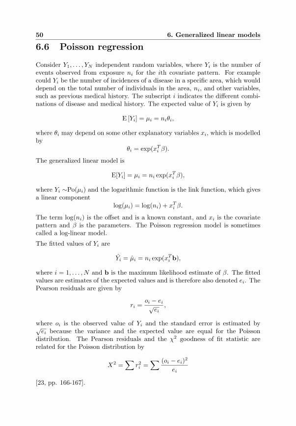
50 6. Generalized linear models
6.6 Poisson regression
Consider Y1, . . . , YN independent random variables, where Yi is the number ofevents observed from exposure ni for the ith covariate pattern. For examplecould Yi be the number of incidences of a disease in a specific area, which woulddepend on the total number of individuals in the area, ni, and other variables,such as previous medical history. The subscript i indicates the different combi-nations of disease and medical history. The expected value of Yi is given by
E [Yi] = µi = niθi,
where θi may depend on some other explanatory variables xi, which is modelledby
θi = exp(xTi β).
The generalized linear model is
E[Yi] = µi = ni exp(xTi β),
where Yi ∼Po(µi) and the logarithmic function is the link function, which givesa linear component
log(µi) = log(ni) + xTi β.
The term log(ni) is the offset and is a known constant, and xi is the covariatepattern and β is the parameters. The Poisson regression model is sometimescalled a log-linear model.
The fitted values of Yi are
Yi = µi = ni exp(xTi b),
where i = 1, . . . , N and b is the maximum likelihood estimate of β. The fittedvalues are estimates of the expected values and is therefore also denoted ei. ThePearson residuals are given by
ri =oi − ei√
ei,
where oi is the observed value of Yi and the standard error is estimated by√ei because the variance and the expected value are equal for the Poisson
distribution. The Pearson residuals and the χ2 goodness of fit statistic arerelated for the Poisson distribution by
X2 =∑
r2i =∑ (oi − ei)2
ei
[23, pp. 166-167].

6.6 Poisson regression 51
Deviance for a Poisson model
Let the response variables Yi ∼ Po(λi), i = 1, . . . , N , be independent, then thelog-likelihood function is
`(β; y) =∑
yi log(λi)−∑
λi −∑
log(yi!).
The maximum value of the likelihood function is
`(bmax; y) =∑
yi log(yi)−∑
yi −∑
log(yi!),
where the maximum likelihood estimate of λi = yi. The log-likelihood functionof the model of interest with p parameters evaluated at the maximum likelihoodestimate for β, b, is
`(b; y) =∑
yi log(yi)−∑
yi −∑
log(yi!)
The deviance for the Poisson model is defined as
D = 2[`(bmax; y)− `(b; y)]
= 2[∑
yi log(yi/yi)−∑
(yi − yi)]
= 2∑[
oi log
(oiei
)− (oi − ei)
],
where oi is the observed value yi and ei is the estimated expected value yi. Thedeviance residuals are
di = sign(oi − ei)√[
oi log
(oiei
)− (oi − ei)
],
for i = 1, . . . , N . The deviance and the deviance residuals are related as D =∑d2i , and the deviance and the χ2 goodness of fit statistic are also related
approximately in the following way
D ≈ 2
N∑
i=1
[(oi − ei) +
1
2
(oi − ei)2ei
− (oi − ei)]
=
N∑
i=1
(oi − ei)2ei
= X2,
where the Taylor series expansion o log(oe
)= (o − e) + 1
2(o−e)2e + . . . is used.
Both the deviance and the χ2 statistic can be used as a measure of goodness offit. They can be obtained from the data and the fitted model and are comparedwith the χ2 distribution with N − q degrees of freedom, where q is the numberof estimated parameters [23, pp. 83-84,166-168].


Chapter 7
State space models
With state space models we consider time series, which are the output of a dy-namic system affected by random noise. State space models are a flexible classof models, that can be used in a wide variety of applications including, whenthe time series are non-stationary, have structural changes or display irregularpatterns. The model can consists of a combination of several components; forinstance trend, seasonal or regressive components, that gives a natural inter-pretation of the parameters and the output. Recursive computations of theconditional distribution of the parameters of interest given the available infor-mation are used for estimation and forecasting [24, p. 31].
Let (Yt)t≥1 be a time series. The joint distribution of (Y1, . . . , Yt) for any t ≥ 1is defined using Markovian dependence structure,because assumptions of inde-pendence or exchangeability would make time irrelevant, which is often not truefor most time series. The time series (Yt)t≥1 is a Markov chain if
π(yt|y1:t−1) = π(yt|yt−1)
for any t > 1, and the joint finite-dimensional distribution is given by
π(y1:t) = π(y1) ·t∏
j=2
π(yj |yj−1).
In many situations it is not appropriate to assume a Markovian structure forthe observations. Therefore it is assumed in state space models that there isa state process, which is an unobservable Markov chain (θt), and that Yt is ameasurement of θt affected by random disturbance. Figure 7.1 shows a directedacyclic graph, which illustrates the dependence structure in a state space model.The graph can be used to deduce conditional independence properties of randomvariables, for example variables A and B are conditionally independent given athird set C, if and only if C separates A and B [24, pp. 39-41].
53

54 7. State space models
θ0- θ1
- θ2- · · · - θt−1
- θt- θt+1
- · · ·
?Y1
?Y2
?Yt−1
?Yt
?Yt+1
1
Figure 7.1: Dependence structure in a state space model [24, p. 41]
Definition 7.1 (State space model)A state space model consists of to time series: An Rp-valued time-series(θt : t = 0, 1, . . .), and (Yt : t = 1, 2, . . .) an Rm-valued time series. The timeseries satisfy the following assumptions:
1. (θt) is a Markov chain.
2. Conditionally on (θt), the Yt’s are independent and Yt depends on θt only.
[24, p. 40]. �
The joint distribution of (θ0, θ1, . . . , θt, Y1, . . . , Yt) for any t > 0 is then given by
π(θ0:t, y1:t) = π(θ0) ·t∏
j=1
π(θj |θj−1)π(yj |θj). (7.1)
This distribution can be used to derive distributions of interest by conditioningor marginalization. If the states are discrete-valued random variables the statespace models is sometimes called hidden Markov models [24, pp. 40-41].
7.1 Dynamic linear models
Dynamic linear models, also known as Gaussian linear state space models, area particular class of state space models. Let (Yt)t≥1 be a time series, then adynamic linear model is defined as follows.
Definition 7.2 (Dynamic linear model)A dynamic linear model (DLM) is defined by a Normal prior distribution
θ0 ∼ Np(m0, C0) (7.2a)
for the p-dimensional state space vector at time t = 0 and the pair of equationsfor each time t ≥ 1,
Yt = Ftθt + vt , vt ∼ Nm(0, Vt) (7.2b)
θt = Gtθt−1 + wt , wt ∼ Np(0,Wt) (7.2c)

7.2 State estimation and forecasting 55
where Ft is a known m× p-matrix and Gt is a known p× p-matrix, and (vt)t≥1and (wt)t≥1 are two independent sequences of independent Gaussian randomvectors with zero mean and known variance matrices (Vt)t≥1 and (Wt)t≥1, re-spectively. The state vector at time t = 0, θ0 is independent of (vt) and (wt).Equation (7.2b) is the observation equation and equation (7.2c) is the stateequation or system equation [24, p. 41]. �
In dynamic linear models it is assumed, that the distribution is Gaussian, whichis true in many applications [24, p. 42].
7.2 State estimation and forecasting
State space models can be used in many applications. Let a model be specified bythe densities π(yt|θt) and π(θt|θt−1). The main objective of state space models isto make inference on unobserved states and predict future events based on pastevents. Calculating the conditional distribution given the previous informationsis used for estimation and forecasting. The conditional densities π(θs|y1:t) arecalculated to estimate the states. This involves three different tasks, filteringis when s = t, state predicting is when s > t, and smoothing is when s < t.Filtering is done by calculating the conditional density π(θt|y1:t), which for aDLM is carried out by the Kalman filter, that update the inference of the stateswhen new observations are obtained. Filtering can be be implemented as arecursive algorithm. When smoothing the conditional distribution of θ1:t giveny1:t is calculated, which also can be implemented as a recursive algorithm.
The one-step-ahead forecasting is prediction of θt+1 and Yt+1 based on the pre-vious observations y1:t. First the state θt+1 is estimated and then the observationYt+1 is estimated. The state predictive density of the one-step-ahead forecast isgiven by π(θt+1|y1:t), and the one-step-ahead predictive density is π(yt+1|y1:t).Similarly the k-step-ahead forecasts Yt+k can be calculated by first estimatingthe state θt+k for k ≥ 1 and then predicting Yt+k. The state predictive densityof the k-step-ahead forecast is given by π(θt+k|y1:t), and the k-step-ahead pre-dictive density is π(yt+k|y1:t). The forecasts become more uncertain for largevalues of k [24, pp. 49-51].
7.2.1 Filtering
In this section the recursive steps in calculations of the filtering densities π(θt|y1:t)in a state space model is described. The filtering and predictive densities can becalculated recursively because of the assumptions in definition 7.1. The followingproposition present the filtering recursive steps.

56 7. State space models
Proposition 7.1 (Filtering recursions)For a general state space model specified by definition 7.1 the following is true
(i) The one-step-ahead predictive density for θt is calculated using the filtereddensity π(θt−1|y1:t−1), which gives
π(θt|y1:t−1) =
∫π(θt|θt−1)π(θt−1|y1:t−1)dθt−1. (7.3a)
(ii) The one-step-ahead predictive density for Yt is calculated using the predic-tive density for the states as
π(yt|y1:t−1) =
∫π(yt|θt)π(θt|y1:t−1)dθt. (7.3b)
(iii) The filtering density can be calculated using (i) and (ii)
π(θt|y1:t) =π(yt|θt)π(θt|y1:t−1)
π(yt|y1:t−1). (7.3c)
Proof. The state θt is conditionally independent of Y1:t−1 given θt−1. Then (i)is proved by
π(θt|y1:t−1) =
∫π(θt−1, θt|y1:t−1)dθt−1
=
∫π(θt|θt−1, y1:t−1)π(θt−1|y1:t−1)dθt−1
=
∫π(θt|θt−1)π(θt−1|y1:t−1)dθt−1.
The observation Yt is conditionally independent of Y1:t−1 given θt and (ii) isproved by
π(yt|y1:t−1) =
∫π(yt, θt|y1:t−1)dθt
=
∫π(yt|θt, y1:t−1)π(θt|y1:t−1)dθt
=
∫π(yt|θt)π(θt|y1:t−1)dθt.
The proof of (iii) uses Bayes’ rule and the conditional independence of Yt andY1:t−1 given θt. Then
π(θt|y1:t) =π(θt|y1:t−1)π(yt|θt, y1:t−1)
π(yt|y1:t−1)
=π(θt|y1:t−1)π(yt|θt)
π(yt|y1:t−1).

7.2 State estimation and forecasting 57
[24, pp. 51-53].
7.2.2 Kalman filter for DLM
Proposition 7.1 showed the principle of filtering and forecasting, but calculatingthe conditional distributions required is not always easy. One of the advantagesof the DLM is that all the relevant distributions are Gaussian, which means thatthey can be completely determined by their means and variances. The followingproposition shows this result.
Proposition 7.2 (Kalman filter)Let a DLM be defined by definition 7.2, let the prior distribution be given byθ0 ∼ N(m0, C0), and let
θt−1|y1:t−1 ∼ N (mt−1, Ct−1) .
Then the following statements are true.
(i) The one-step-ahead predictive distribution of θt given y1:t−1 is Gaussianwith parameters
at = E[θt|y1:t−1] = Gtmt−1,
Rt = Var[θt|y1:t−1] = GtCt−1GTt +Wt.
(ii) The one-step-ahead predictive distribution of Yt given y1:t−1 is Gaussianwith parameters
ft = E[Yt|y1:t−1] = Ftat,
Qt = Var[Yt|y1:t−1] = FtRtFTt + Vt.
(iii) The filtering distribution of θt given y1:t is Gaussian with parameters
mt = E[θt|y1:t] = at +RtFTt Q−1t et,
Ct = Var[θt|y1:t] = Rt −RtFTt Q−1t FtRt,
where et = Yt − ft is the forecast error.
Proof. The joint distribution of (θ0, θ1, . . . , θt, Y1, . . . , Yt) is given by equation(7.1), where the marginal and conditional distributions are Gaussian. Thus itfollows that the joint distribution for the random vector (θ0, θ1, . . . , θt, Y1, . . . , Yt)is also Gaussian for any t ≥ 0, and the distribution of any subvector or con-ditional distribution of some components given others is also Gaussian. Thismeans, that it is enough to compute the means and variances of the predic-tive distributions and the filtering distributions, because they are Gaussian dis-tributed.

58 7. State space models
Let θt|y1:t−1 ∼ N(at, Rt), then (i) is proved using equation (7.2c), and at andRt can be specified as
at = E[θt|y1:t−1] = E[E[θt|θt−1, y1:t−1]
∣∣∣y1:t−1]
= E[Gtθt−1|y1:t−1] = Gtmt−1,
and
Rt = Var[θt|y1:t−1]
= E[Var[θt|θt−1, y1:t−1]
∣∣∣y1:t−1]
+ Var[E[θt|θt−1, y1:t−1]
∣∣∣y1:t−1]
= Wt + Var[Gtθt−1|y1:t−1]
= Wt +GtCt−1GTt .
Let Yt|y1:t−1 ∼ N(ft, Qt), then (ii) is proved using equation (7.2b), and ft andQt can be specified as
ft = E[Yt|y1:t−1] = E[E[Yt|θt, y1:t−1]
∣∣∣y1:t−1]
= E[Ftθt|y1:t−1] = Ftat,
and
Qt = Var[Yt|y1:t−1]
= E[Var[Yt|θt, y1:t−1]
∣∣∣y1:t−1]
+ Var[E[Yt|θt, y1:t−1]
∣∣∣y1:t−1]
= Vt + Var[Ftθt|y1:t−1]
= Vt + FtRtFTt .
The conditional covariance of Yt and θt is given by
Cov[Yt, θt|y1:t−1] = Cov[Ftθt + vt, θt|y1:t−1]
= FtCov[θt, θt|y1:t−1] + FtCov[vt, θt|y1:t−1]
= FtVar[θt|y1:t−1]
= FtRt,
because Cov[vt, θt|y1:t−1] = 0 since vt and θt are conditionally independent.From multivariate Gaussian theory the distribution of Yt and θt given y1:t−1 is
(Ytθt
∣∣∣∣ y1:t−1)∼ N
((ftat
),
{Qt FtRt
RtFTt Rt
}).
This means that θt is Gaussian with the following expected value and varianceconditionally on y1:t
mt = E[θt|yt, y1:t−1] = at +RtFTt Q−1t (yt − ft),

7.2 State estimation and forecasting 59
and
Ct = Var[θt|yt, y1:t−1] = Rt −RtFTt Q−1t FtRt.
The predictive and filtering distributions can be calculated recursively using theKalman filter beginning at θ0 ∼ N(m0, C0) and then calculate π(θ1), π(y1) andπ(θ1|y1), when new data is obtained [24, pp. 53-55].
Filtering with missing observations
Sometimes time series contain missing observations, which needs to be takinginto account in the filtering recursions. A missing observation does not containany information, so the observation at time t is missing, yt = NA, and
π(θt|y1:t) = π(θt|y1:t−1). (7.5)
Thus the filtering distribution at time t is the one-step-ahead predictive distri-bution at time t− 1. This means that in the filtering recursion, proposition 7.1,equation (7.3c) has to be replaced with equation (7.5). The filtering distributionat time t for a DLM is given by setting the mean value mt = at and the varianceCt = Rt, because θt|y1:t−1 ∼ N(at, Rt) [24, p. 59].
7.2.3 Smoothing
In state space models estimation and forecasting can be applied sequentially,when new data are collected. Often information about a time series Yt is avail-able for a period of time, and it is desired to retrospectively reconstruct thebehavior of the system. This can be done using a backward recursive algorithm,which compute the conditional distribution of θt given y1:T for any t < T , start-ing from the filtering distribution π(θT |y1:T ) and estimating the states back-wards. This method is called smoothing and is presented for general state spacemodels in the following proposition.
Proposition 7.3 (Smoothing recursion)For a general state space model specified by definition 7.1 the following is true
(i) The state system (θ0, . . . , θT ) given y1:T has backward transition probabi-lities specified by
π(θt|θt+1, y1:T ) =π(θt+1|θt)π(θt|y1:t)
π(θt+1|y1:t).

60 7. State space models
(ii) Conditional on y1:T the smoothing distribution of θt can be calculated usingthe backward recursion in t starting from π(θT |y1:T )
π(θt|y1:T ) = π(θt|y1:t)∫
π(θt+1|θt)π(θt+1|y1:t)
π(θt+1|y1:T )dθt+1.
Proof. The state θt and the observation Yt+1:T are conditionally independentgiven θt+1, and given θt, θt+1 and Y1:T are conditionally independent. Then (i)is proved using Bayes formula
π(θt|θt+1, y1:T ) = π(θt|θt+1, y1:t)
=π(θt|y1:t)π(θt+1|θt, y1:t)
π(θt+1|y1:t)
=π(θt|y1:t)π(θt+1|θt)
π(θt+1|y1:t).
The density π(θt, θt+1|y1:T ) with respect to θt+1 is marginalized to prove (ii)
π(θt|y1:T ) =
∫π(θt, θt+1|y1:T )dθt+1
=
∫π(θt+1|y1:T )π(θt|θt+1, y1:T )dθt+1
=
∫π(θt+1|y1:T )
π(θt+1|θt)π(θt|y1:t)π(θt+1|y1:t)
dθt+1
= π(θt|y1:t)∫π(θt+1|θt)
π(θt+1|y1:T )
π(θt+1|y1:t)dθt+1.
The smoothing recursion can be expressed using the means and variances of thesmoothing distributions for a DLM. This is presented in the following proposi-tion.
Proposition 7.4 (Kalman smoother)Given a DLM as defined in definition 7.2, if θt+1|y1:T ∼ N(st+1, St+1), thenθt|y1:T ∼ N(st, St), where
st = mt + CtGTt+1R
−1t+1(st+1 − at+1)
St = Ct − CtGTt+1R−1t+1(Rt+1 − St+1)R−1t+1Gt+1Ct.
Proof. The conditional distribution of θt given y1:T is Gaussian, because ofproperties of the multivariate Gaussian distribution, which means that it is

7.2 State estimation and forecasting 61
sufficient to calculate the mean and the variance. The mean value of θt giveny1:T is
st = E[θt|y1:T ] = E[E[θt|θt+1, y1:T ]
∣∣∣y1:T]
= E[E[θt|θt+1, y1:t]
∣∣∣y1:T],
since θt and yt+1:T are conditional independent given θt+1, thus
π(θt|θt+1, y1:T ) = π(θt|θt+1, y1:t).
The variance of θt given y1:T is
St = Var[θt|y1:T ] = E[Var[θt|θt+1, y1:T ]
∣∣∣y1:T]
+ Var[E[θt|θt+1, y1:T ]
∣∣∣y1:T]
= E[Var[θt|θt+1, y1:t]
∣∣∣y1:T]
+ Var[E[θt|θt+1, y1:t]
∣∣∣y1:T].
The likelihood π(θt+1|θt, y1:t) = π(θt+1|θt) is θt+1|θt ∼ N(Gt+1θt,Wt+1) givenby the state equation (7.2c) and the prior θt|y1:t ∼ N(mt, Ct). Because boththe likelihood and prior are Gaussian distributed the posterior is also Gaussian.The expected value of θt given θt+1 and y1:t can then be written as
E[θt|θt+1, y1:t]
=E[θt|y1:t] + Cov[θt, θt+1|y1:t]Var[θt+1|y1:t]−1(θt+1 − E[θt+1|y1:t])=mt + CtG
Tt+1R
−1t+1(θt+1 − at+1),
since
Cov[θt, θt+1|y1:t] = Cov[θt, Gt+1θt + vt|y1:t]= Var[θt|y1:t]GTt+1
= CtGTt+1.
The variance of θt given θt+1 and y1:t is
Var[θt|θt+1, y1:t]
=Var[θt|y1:t]− Cov[θt, θt+1|y1:t]Var[θt+1|y1:t]−1Cov[θt, θt+1|y1:t]T
=Ct − CtGTt+1R−1t+1Gt+1C
Tt ,
and
Var[E[θt|θt+1, y1:t]
∣∣∣y1:T]
= CtGTt+1R
−1t+1Var[θt+1|y1:T ]R−1t+1Gt+1C
Tt .
It is assumed that E[θt+1|y1:T ] = st+1 and Var[θt+1|y1:T ] = St+1. The meanvalue and variance of θt given y1:T is then
st = E[E[θt|θt+1, y1:t]
∣∣∣y1:T]
= mt + CtGTt+1R
−1t+1(st+1 − at+1)

62 7. State space models
and
St = E[Var[θt|θt+1, y1:t]
∣∣∣y1:T]
+ Var[E[θt|θt+1, y1:t]
∣∣∣y1:T]
= Ct − CtGTt+1R−1t+1Gt+1Ct + CtG
Tt+1R
−1t+1St+1R
−1t+1Gt+1Ct
= Ct − CtGTt+1R−1t+1(Rt+1 − St+1)R−1t+1Gt+1Ct.
The distribution of θt|y1:T can be computed recursively backwards beginning att = T − 1 and then proceed with t = T − 2 and so on, given thatθt|y1:T ∼ N(sT = mT , ST = CT ) [24, pp. 60-62],[25, p. 114].
7.2.4 Forecasting
In state space models forecasting future values of the observations, Yt+k, or ofthe state vectors, θt+k, of a time series, when knowing the time series up to timet is one of the main tasks. The forecast can be computed recursively as new ob-servations are obtained. The one-step-ahead predictive distribution for a generalstate space model was presented in proposition 7.1 and for a DLM in proposition7.2. Sometimes one is interested in forecasting k-steps-ahead into the future.The following proposition, proposition 7.5, present the distributions of the stateand the observation at time t+ k. The filtering distribution at time t acts as aninitial distribution for the forecast distribution. This means that in a state spacemodel the distribution containing information about present and future states(θt+k)k≥0 and future observations (Yt+k)k≥1 are the conditional distributionsπ(θt+k|θt+k−1) and π(yt+k|θt+k), and the initial distribution π(θt|y1:t). For aDLM it is sufficient to calculate the mean and the variance of π(θt|y1:t), mt andCt, for prediction of future values. Figure 7.2 illustrates, that the observations
θt
Y1:t
- θt+1- · · · - θt+k
? ?Yt+k
1
Figure 7.2: Forecasting of states and observations
Y1:t gives information about θt, which gives information about future values ofthe time series. In the next proposition, proposition 7.5, the forecast recursionsfor a general state space model is presented.

7.2 State estimation and forecasting 63
Proposition 7.5 (Forecasting recursion)For a general state space model specified by definition 7.1 the following is truefor any k > 0.
(i) The k-step-ahead forecast distribution of the state is
π(θt+k|y1:t) =
∫π(θt+k|θt+k−1)π(θt+k−1|y1:t)dθt+k−1.
(ii) The k-step-ahead forecast distribution of the observation is
π(yt+k|y1:t) =
∫π(yt+k|θt+k)π(θt+k|y1:t)dθt+k.
Proof. The state θt+k is conditionally independent of Y1:t given θt+k−1, and (i)is proved by
π(θt+k|y1:t) =
∫π(θt+k, θt+k−1|y1:t)dθt+k−1
=
∫π(θt+k|θt+k−1, y1:t)π(θt+k−1|y1:t)dθt+k−1
=
∫π(θt+k|θt+k−1)π(θt+k−1|y1:t)dθt+k−1.
The observation Yt+k is conditionally independent of Y1:t given θt+k, and (ii) isproved by
π(yt+k|y1:t) =
∫π(yt+k, θt+k|y1:t)dθt+k
=
∫π(yt+k|θt+k, y1:t)π(θt+k|y1:t)dθt+k
=
∫π(yt+k|θt+k)π(θt+k|y1:t)dθt+k.
For DLM it is sufficient to calculate the means and variances of the forecastdistributions, since all the distributions are Gaussian. The following propositionpresent the forecast recursions for a DLM.
Proposition 7.6Let a DLM be defined by definition 7.2, then the following is true for k ≥ 0.
(i) The state θt+k|y1:t ∼ N(at+k, Rt+k), with
at+k = E[θt+k|y1:t] = Gt+kat+k−1,
Rt+k = Var[θt+k|y1:t] = Gt+kRt+k−1GTt+k +Wt+k,
where at+0 = mt and Rt+0 = Ct.
64 7. State space models
(ii) The observation Yt+k|y1:t ∼ N(ft+k, Qt+k), with
ft+k = E[Yt+k|y1:t] = Ft+kat+k,
Qt+k = Var[Yt+k|y1:t] = Ft+kRt+kFTt+k + Vt+k.
Proof. The proposition is proved using induction. For k = 1 the propositionis equivalent to proposition 7.2 (i) and (ii), and thereby the result holds. Fork > 1 (i) and (ii) is proved by
at+k = E[θt+k|y1:t]= E
[E[θt+k|θt+k−1, y1:t]
∣∣∣y1:t]
= E[Gt+kθt+k−1|y1:t]= Gt+kat+k−1,
Rt+k = Var[θt+k|y1:t]= Var
[E[θt+k|θt+k−1, y1:t]
∣∣∣y1:t]
+ E[Var[θt+k|θt+k−1, y1:t]
∣∣∣y1:t]
= Var[Gt+kθt+k−1|y1:t] +Wt+k
= Gt+kRt+k−1GTt+k +Wt+k,
ft+k = E[Yt+k|y1:t]= E
[E[Yt+k|θt+k, y1:t]
∣∣∣y1:t]
= E[Ft+kθt+k|y1:t]= Ft+kat+k,
Qt+k = Var[Yt+k|y1:t]= Var
[E[Yt+k|θt+k, y1:t]
∣∣∣y1:t]
+ E[Var[Yt+k|θt+k, y1:t]
∣∣∣y1:t]
= Var[Ft+kθt+k|y1:t] + Vt+k
= Ft+kRt+kFTt+k + Vt+k.
The forecasts become more imprecise as k gets larger, because more uncertaintyenters the system. In the following the forecast error is defined.

7.3 The innovation process and model checking 65
7.3 The innovation process and model checking
The one-step-ahead forecasts ft = E[Yt|Y1:t−1] for DLMs are given by theKalman filter, proposition 7.2, and the forecast error is defined as
et = Yt − E[Yt|Y1:t−1]
= Yt − ft= Ftθt + vt − Ftat= Ft(θt − at) + vt.
In the following proposition different properties of the sequence (et)t≥1 of fore-cast errors are presented.
Proposition 7.7The sequence (et)t≥1 of forecast errors of a DLMs has the following properties.
(i) The expected value of et is zero, i.e. E[et] = 0
(ii) The random error vector et is uncorrelated with any function of Y1, . . . , Yt−1,i.e. Cov[et, Z] = 0, where Z = g(Y1, . . . , Yt−1).
(iii) The error et and the observation Ys are uncorrelated for any s < t.
(iv) The errors et and es are uncorrelated for any s < t.
(v) The error et is a linear function of Y1, . . . , Yt.
(vi) The process (et)t≥1 of forecast errors is a Gaussian process.
Proof. (i) The expected value of et is
E[et] = E[E[Yt − ft|Y1:t−1]
]= 0
using that E[Y ] = E[E[Y |X]
].
(ii) The covariance of et and Z is
Cov[et, Z] = E[etZ]
= E[E[etZ|Y1:t−1]
]
= E[E[et|Y1:t−1]Z
]
= 0.
(iii) For univariate observations it follows from (ii) by setting Z = Ys. Or elseuse (ii) on each component of Ys.

66 7. State space models
(iv) Again for univariate observations it follows from (ii) by setting Z = es.Or else use (ii) on each component of es.
(v) The error et is a linear function of Y1, . . . , Yt, because ft = E[Yt|Y1:t−1]is a linear function of Y1, . . . , Yt−1, since Y1, . . . , Yt have a joint Gaussiandistribution.
(vi) From (v) it follows that for any t the sequence (e1, . . . , et) is a lineartransformation of (Y1, . . . , Yt), which has a joint Gaussian distribution.Then (e1, . . . , et) has a joint Gaussian distribution, and the process (et)t≥1is Gaussian, since all finite distributions are Gaussian.
The observation Yt = ft + et is the sum of a component ft, which is predictablefrom past observations, and a component, et, independent of the past and con-taining the new information given by Yt. Because of this the forecast errors etare also called innovations.
The sequence of standardized innovations for univariate observations is given by
et =et√Qt,
which is Gaussian white noise. Gaussian white noise are independent, identicallydistributed random variables with zero mean. The standardized innovationscan be used to check the model assumptions. This means that, if the modelassumptions are correct, then the sequence e1, . . . , et should be a sample of sizet from a standard normal distribution. A QQ-plot can be used to check if thestandard innovations are normal distributed, and the empirical autocorrelationfunction to check if they are uncorrelated [24, pp. 73-75].
7.4 Model specification
In this section different classes of DLMs are presented. These classes can beused alone or added together to model univariate time series. Specification ofthe model can be difficult, but one approach is to consider a time series asa combination of different components for instance trend or seasonality. Eachcomponent of the time series is represented by a DLM and then added together ina DLM. A univariate time series (Yt) can be produced as the sum of independentcomponents
Yt = Y1,t + . . .+ Yh,t,

7.4 Model specification 67
where Yi,t represent a component such as trend or seasonality. A DLM can beused to describe the ith component Yi,t for i = 1, . . . , h as
Yi,t = Fi,tθi,t + vi,t , vi,t ∼ N(0, Vi,t)
θi,t = Gi,tθi,t−1 + wi,t , wi,t ∼ N(0,Wi,t),
where each of the pi-dimensional state vectors θi,t are unique and for all i 6= jthe time series (Yi,t, θi,t) and (Yj,t, θj,t) are mutually independent. To achievethe DLM for the time series (Yt) the independent components are added so
Yt =∑hi=1 Yi,t is expressed by the DLM
Yt = Ftθt + vt , vt ∼ N(0, Vt)
θt = Gtθt−1 + wt , wt ∼ Nh(0,Wt),
where the state vector is given by θt = [θ1,t · · · θh,t]T , Ft = [F1,t| · · · |Fh,t], Gtand Wt are given by the block diagonal matrices
Gt =
G1,t
. . .
Gh,t
, Wt =
W1,t
. . .
Wh,t,
and Vt =∑ji=1 Vi,t [24, pp. 88-89].
7.4.1 Trend models
Trend can be described as a smooth development of the series over time, whichcan be modeled using polynomial DLMs. A polynomial model of order n isdefined as a DLM with constant matrices Ft = F and Gt = G, which aredetermined by a forecast function. The forecast function gives the expectedtrend at time t and is defined as
ft+k = E[Yt+k|y1:t] = at+0 + at+1k + . . .+ at+n−1kn−1 , k ≥ 0 (7.6)
where the parameteres at+0, . . . , at+n−1 are linear functions of mt and are in-dependent of k. This means that the forecast function is a polynomial of ordern− 1, and the forecast function can also be written as
ft+k = E[Yt+k|y1:t]= Fat+k
= FGat+k−1= . . .
= FGk−1at+1. (7.7)
Usually small values of n are used. The polynomial model of order n = 1 is therandom walk plus noise model, and the polynomial model of order n = 2 is thelinear growth model [24, p. 89].

68 7. State space models
Random walk plus noise
The random walk plus noise model, also known as a local level model, is apolynomial model of order n = 1, given by the equations
Yt = θt + vt , vt ∼ N(0, V )
θt = θt−1 + wt , wt ∼ N(0,W ),
where (vt) and (wt) are independent, and Ft = Gt = 1. The observations (Yt)are modeled as a level θt plus noise vt, which is affected by random changes overtime [24, p. 42].
The Kalman filter of the random walk plus noise model is given by the one-step-ahead predictive distribution of θt given y1:t−1
θt|y1:t−1 ∼ N(mt−1, Rt = Ct−1 +W ),
the one-step-ahead predictive distribution of Yt given y1:t−1
Yt|y1:t−1 ∼ N(ft = mt−1, Qt = Rt + V ),
and the filtering distribution of θt given y1:t
θt|y1:t ∼ N(mt = mt−1 +Ktet, Ct = KtV ),
where et = Yt−ft and Kt = RtQ−1t . The behavior of the process (Yt) is affected
by the signal-to-noise ratio, which is the ratio between the two error variancesr = W/V . The structure of the estimation and forecasting reflect this ratio.The mean value of the filtering distribution can be written as
mt = mt−1 +Ktet = mt−1 +Kt(yt − ft)= mt−1 +Kt(yt −mt−1) = mt−1 +Ktyt −Ktmt−1= Ktyt + (1−Kt)mt−1.
This shows that mt is a weighted average of yt and mt−1. The weight of thecurrent observation yt is called the adaptive coefficient and is given by
Kt =RtQt
=Ct−1 +W
Ct−1 +W + V,
where 0 < Kt < 1. For any C0, the adaptive coefficient Kt is small and theobservation yt receives little weight, if the signal-to-noise ratio is small. On theother hand if the variance of the error of the observation V = 0, then Kt = 1,and the one-step-ahead forecast is given by the previous data point, thus mt = yt[24, pp. 55-56].
In summary if the signal-to-noise ratio is small, the model is trusted more thannew data points, and if the signal-to-noise ratio is large, new data points are

7.4 Model specification 69
90 3 Model specification
(Yt) is greatly influenced by the signal-to-noise ratio r = W/V , the ratio be-tween the two error variances. Figure 3.1 shows some simulated trajectoriesof (Yt) and (µt) for different values of the ratio r (see Problem 3.1).
0 10 20 30 40 50
510
15
20
log10 r = 0.1
0 10 20 30 40 50
510
15
20
log10 r = 1
0 10 20 30 40 50
510
15
20
log10 r = 10
0 10 20 30 40 50
510
15
20
log10 r = 100
Fig. 3.1. Trajectories of the random walk plus noise, for different values of thesignal-to-noise ratio. The trajectory of the state µt is shown in gray and is the samein the four plots
The k-steps-ahead predictive distribution for this simple model is
Yt+k|y1:t ∼ N(mt, Qt(k)) , k ≥ 1 , (3.7)
where Qt(k) = Ct+∑kj=1Wt+j+Vt+k = Ct+kW+V . We see that the forecast
function ft(k) = E(Yt,k|y1:t) = mt is constant (as a function of k). For thisreason this model is also referred to as the steady model. The uncertainty onthe future observations is summarized by the variance Qt(k) = Ct+ kW +V ,and we clearly see that it increases as the time horizon t+k gets further away.
The controllability and observability matrices of the model are
C =[W 1/2
],
O = F = [1],
which are trivially of full rank, as long as W > 0. It follows from the resultsof Section 2.11 that the Kalman filter for this model is asymptotically stable,with Rt, Ct, and the gain matrix Kt converging to limiting values R,C, andK, respectively. It can be shown (see West and Harrison; 1997, Theorem 2.3)that
(a) r = 0.1
90 3 Model specification
(Yt) is greatly influenced by the signal-to-noise ratio r = W/V , the ratio be-tween the two error variances. Figure 3.1 shows some simulated trajectoriesof (Yt) and (µt) for different values of the ratio r (see Problem 3.1).
0 10 20 30 40 50
510
15
20
log10 r = 0.1
0 10 20 30 40 50
510
15
20
log10 r = 1
0 10 20 30 40 50
510
15
20
log10 r = 10
0 10 20 30 40 50
510
15
20
log10 r = 100
Fig. 3.1. Trajectories of the random walk plus noise, for different values of thesignal-to-noise ratio. The trajectory of the state µt is shown in gray and is the samein the four plots
The k-steps-ahead predictive distribution for this simple model is
Yt+k|y1:t ∼ N(mt, Qt(k)) , k ≥ 1 , (3.7)
where Qt(k) = Ct+∑kj=1Wt+j+Vt+k = Ct+kW+V . We see that the forecast
function ft(k) = E(Yt,k|y1:t) = mt is constant (as a function of k). For thisreason this model is also referred to as the steady model. The uncertainty onthe future observations is summarized by the variance Qt(k) = Ct+ kW +V ,and we clearly see that it increases as the time horizon t+k gets further away.
The controllability and observability matrices of the model are
C =[W 1/2
],
O = F = [1],
which are trivially of full rank, as long as W > 0. It follows from the resultsof Section 2.11 that the Kalman filter for this model is asymptotically stable,with Rt, Ct, and the gain matrix Kt converging to limiting values R,C, andK, respectively. It can be shown (see West and Harrison; 1997, Theorem 2.3)that
(b) r = 1
90 3 Model specification
(Yt) is greatly influenced by the signal-to-noise ratio r = W/V , the ratio be-tween the two error variances. Figure 3.1 shows some simulated trajectoriesof (Yt) and (µt) for different values of the ratio r (see Problem 3.1).
0 10 20 30 40 50
510
15
20
log10 r = 0.1
0 10 20 30 40 50
510
15
20
log10 r = 1
0 10 20 30 40 50
510
15
20
log10 r = 10
0 10 20 30 40 505
10
15
20
log10 r = 100
Fig. 3.1. Trajectories of the random walk plus noise, for different values of thesignal-to-noise ratio. The trajectory of the state µt is shown in gray and is the samein the four plots
The k-steps-ahead predictive distribution for this simple model is
Yt+k|y1:t ∼ N(mt, Qt(k)) , k ≥ 1 , (3.7)
where Qt(k) = Ct+∑kj=1Wt+j+Vt+k = Ct+kW+V . We see that the forecast
function ft(k) = E(Yt,k|y1:t) = mt is constant (as a function of k). For thisreason this model is also referred to as the steady model. The uncertainty onthe future observations is summarized by the variance Qt(k) = Ct+ kW +V ,and we clearly see that it increases as the time horizon t+k gets further away.
The controllability and observability matrices of the model are
C =[W 1/2
],
O = F = [1],
which are trivially of full rank, as long as W > 0. It follows from the resultsof Section 2.11 that the Kalman filter for this model is asymptotically stable,with Rt, Ct, and the gain matrix Kt converging to limiting values R,C, andK, respectively. It can be shown (see West and Harrison; 1997, Theorem 2.3)that
(c) r = 10
90 3 Model specification
(Yt) is greatly influenced by the signal-to-noise ratio r = W/V , the ratio be-tween the two error variances. Figure 3.1 shows some simulated trajectoriesof (Yt) and (µt) for different values of the ratio r (see Problem 3.1).
0 10 20 30 40 50
510
15
20
log10 r = 0.1
0 10 20 30 40 50
510
15
20
log10 r = 1
0 10 20 30 40 50
510
15
20
log10 r = 10
0 10 20 30 40 505
10
15
20
log10 r = 100
Fig. 3.1. Trajectories of the random walk plus noise, for different values of thesignal-to-noise ratio. The trajectory of the state µt is shown in gray and is the samein the four plots
The k-steps-ahead predictive distribution for this simple model is
Yt+k|y1:t ∼ N(mt, Qt(k)) , k ≥ 1 , (3.7)
where Qt(k) = Ct+∑kj=1Wt+j+Vt+k = Ct+kW+V . We see that the forecast
function ft(k) = E(Yt,k|y1:t) = mt is constant (as a function of k). For thisreason this model is also referred to as the steady model. The uncertainty onthe future observations is summarized by the variance Qt(k) = Ct+ kW +V ,and we clearly see that it increases as the time horizon t+k gets further away.
The controllability and observability matrices of the model are
C =[W 1/2
],
O = F = [1],
which are trivially of full rank, as long as W > 0. It follows from the resultsof Section 2.11 that the Kalman filter for this model is asymptotically stable,with Rt, Ct, and the gain matrix Kt converging to limiting values R,C, andK, respectively. It can be shown (see West and Harrison; 1997, Theorem 2.3)that
(d) r = 100
Figure 7.3: Random walk plus noise models for different values of the signal-to-noiseratio. The observations (Yt) is the black line and the state (θt) is the gray line [24, p.90].
trusted more than the model. This is illustrated in figure 7.3, where a randomwalk plus noise model is shown with different signal-to-noise ratios. In figure7.3(a) the signal-to-noise ratio is small, and the model is trusted more thanthe data, but in figure 7.3(d) the signal-to-noise ratio is large, and the data istrusted more than the model.
The k-step-ahead predictive distribution is given by
Yt+k|y1:t ∼ N(mt, Qt+k) , k ≥ 1,
where
Qt+k = Ct +
k∑
j=1
Wt+j + Vt+k
= Ct + kW + V,
since the terms in the error sequence (wt) are independent. The forecast functionof the model is constant, ft+k = E[Yt+k|y1:t] = mt, which is why the model isalso called a steady model. The variance Qt+k contain the uncertainty on thefuture observations, which increases linearly as k gets larger. The random walkplus noise model can be used to model data without any clear trend or seasonalvariability [24, p. 90].
70 7. State space models
7.4.2 Linear growth model
A linear growth model is also called a local linear trend model. The modelis similar to the random walk plus noise model, but a time-varying slope isincluded in the state dynamics. This is defined in the following equations
Yt = µt + vt, vt ∼ N(0, V )
µt = µt−1 + βt−1 + wt,1, wt,1 ∼ N(0, σ2µ),
βt = βt−1 + wt,2, wt,2 ∼ N(0, σ2β),
where µt is the local level, βt is the local growth rate and the errors (vt), (wt,1)and (wt,2) are independent. The local level µt is a cumulated random walk.This model is a polynomial DLM of order 2, where the parameters are given by
θt =
[µtβt
], G =
[1 10 1
], W =
[σ2µ 00 σ2
β
], F =
[1 0
].
The variances of the system σ2µ and σ2
β can be equal to zero. In the model acurrent level µt is assumed to change linearly over time, and the growth rate
can also change. Let mt−1 =[µt−1 βt−1
]T, then the one-step-ahead point
forecasts and filtering state estimates are
at = E[θt|y1:t−1] = Gmt−1 =
[1 10 1
] [µt−1βt−1
]=
[µt−1 + βt−1
βt−1
],
ft = E[Yt|y1:t−1] = Ftat =[
1 0][µt−1 + βt−1
βt−1
]= µt−1 + βt−1,
and
mt = at +Ktet =
[µt−1 + βt−1
βt−1
]+
[kt1kt2
]et =
[µt−1 + βt−1 + kt1et
βt−1 + kt2et
]
where Kt =[kt1 kt2
]T. The forecast function is a linear function of k given
by equation (7.7)
ft+k = FGk−1at+1 =[
1 0] [ 1 k − 1
0 1
] [µt + βtβt
]= µt + kβt
[24, pp. 42,96].
7.4.3 Seasonal models
Time series showing cyclical behavior can be modeled using Fourier-form sea-sonal models. Consider a discrete-time periodic function with period s, which is

7.4 Model specification 71
described by the values it takes at time t = 1, 2, . . . , s. Let gt = αt, t = 1, . . . , s,be a function, where the values of gt is repeated every s-times, so gs+1 = α1,gs+2 = α2 and so on. Thus the periodic function gt is related to a s-dimensionalvector α = [α1, . . . , αs]
T . Assume that s is even and let the Fourier frequenciesbe defined as
ωj =2πj
s, j = 0, 1, . . . ,
s
2,
and let s s-dimensional vectors be given by
e0 = [1, 1, . . . , 1]T
c1 = [cos(ω1), cos(2ω1), . . . , cos(sω1)]T
s1 = [sin(ω1), sin(2ω1), . . . , sin(sω1)]T
...cj = [cos(ωj), cos(2ωj), . . . , cos(sωj)]
T
sj = [sin(ωj), sin(2ωj), . . . , sin(sωj)]T
...cs/2 = [cos(ωs/2), cos(2ωs/2), . . . , cos(sωs/2)]T ,
(7.8)
where ss/2 is a vector of zeros and is therefore not considered, andcs/2 = [−1, 1,−1, . . . ,−1, 1]T . The vectors in equation (7.8) are orthogonal andthereby a basis, which means that every vector in Rs can be written as a linearcombination of e0, c1, s1, . . . , cs/2, so
α = a0e0 +
s/2−1∑
j=1
(ajcj + bjsj) + as/2cs/2.
This representation is helpful, since the basis vectors can be extended to periodicfunctions very easily because of the trigonometric functions. For example thetth component of sj is sj(t) = sin(2πtj/2) for any 1 ≤ t ≤ s. The function sjextended to a periodic function is sj(t) = sj(t+ ks), so
sin
(2π(t+ ks)j
s
)= sin
(2πtj
s2πkj
)= sin
2πtj
s.
This means that the extension of sj(t) to any integer t is given by putting t inthe trigometric expression defining sj . The representation of the basis vectors inequation (7.8) goes from smooth to rough, where the constant vector e0 corre-spond to a constant periodic function and cs/2 is the maximal oscillation, wherethe periodic function goes back and forth between −1 and 1. The expression2πtjs , for any j, extends the interval (0, 2πj] and the cosine function cj runs
through a complete period j times as t goes from 1 to s. This means that asj gets higher the rougher cj is, and the function oscillates more frequent. The

72 7. State space models
functions sj and cj with the same oscillation frequency can be grouped together,and the jth harmonic of gt can be defined as
Sj(t) = aj cos(tωj) + bj sin(tωj), j = 1, . . . , s/2,
where bs/2 = 0. Because the mean is modeled separately from the seasonalcomponent, a0 is set to zero, and since the basis vectors are orthogonal the sumof any harmonic over an entire period is zero. Then the function gt can bewritten as
gt =
s/2∑
j=1
Sj(t). (7.9)
Let j be fixed, then the development of Sj as time goes from t to t+ 1 is
Sj(t) 7−→ Sj(t+ 1) = aj cos((t+ 1)ωj) + bj sin((t+ 1)ωj).
If j < s/2 then it is impossible to calculate Sj(t+1) from Sj(t) without knowingaj and bj . But if the conjugate harmonic
S∗j (t) = −aj sin(tωj) + bj cos(tωj)
is also known, then Sj(t+ 1) can be calculated explicitly. So
Sj(t+ 1) = aj cos((t+ 1)ωj) + bj sin((t+ 1)ωj)
= aj cos(tωj + ωj) + bj sin(tωj + ωj)
= aj(cos(tωj) cos(ωj)− sin(tωj) sin(ωj))
+bj(sin(tωj) cos(ωj) + cos(tωj) sin(ωj))
= aj cos(tωj) cos(ωj)− aj sin(tωj) sin(ωj)
+bj sin(tωj) cos(ωj) + bj cos(tωj) sin(ωj)
= (aj cos(tωj) + bj sin(tωj)) cos(ωj)
+(−aj sin(tωj) + bj cos(tωj)) sin(ωj)
= Sj(t) cos(ωj) + S∗j (t) sin(ωj). (7.10)
Similarly the conjugate harmonic S∗j can be computed as
S∗j (t+ 1) = S∗j (t) cos(ωj) + Sj(t) sin(ωj). (7.11)
By merging equation (7.10) and equation (7.11) then[Sj(t+ 1)S∗j (t+ 1)
]=
[cos(ωj) sin(ωj)− sin(ωj) cos(ωj)
] [Sj(t)S∗j (t)
].
The jth harmonic fits in a DLM by considering the bivariate state vector[Sj(t), S
∗j (t)]T with evolution matrix
Hj =
[cos(ωj) sin(ωj)− sin(ωj) cos(ωj)
]

7.5 Estimation of unknown parameters 73
and observation matrix F =[
1 0]. When j = s/2, then Ss/2 changes sign
for every unit time increase, since
Ss/2(t+ 1) = cos((t+ 1)π) = − cos(tπ) = −Ss/2(t).
In a DLM this can be seen as s univariate state vector with evolution matrixHs/2 = [−1] and observation matrix F = [1]. To obtain a DLM representa-tion the different harmonics can be combined to attain equation (7.9). This ismanaged by considering the state vector
θt = (S1(t), S∗1 , . . . , S s2−1(t), S s2−1(t)∗, S s
2(t))T , t = 0, 1, . . .
with the evolution matrix
G =
H1 0
. . .
0 H s2
,
and the observation matrix
F =[
1 0 1 0 . . . 0 1].
By letting all the evolution and observation variances be zero, a DLM represen-tation of the seasonal component is achieved [24, pp. 102-106].
7.5 Estimation of unknown parameters
Until now it has been assumed that the system matrices Ft, Gt, Vt and Wt wereknown. This is not always the case, and if not the model matrices are set todepend on a vector of unknown parameters ψ. The vector ψ can be estimatedusing maximum likelihood estimation, MLE.
Let Y1, . . . , Yn be random vectors having distributions depending on an unknownparameter ψ. The joint density of the observations for a specific value of theparameters is given by p(y1, . . . , yn;ψ) and the likelihood of ψ is
L(ψ) = c · p(y1, . . . , yn;ψ),
where c is a constant. For a DLM the joint density of the observations can bewritten in terms of the conditional density of yt given y1:t−1 and the unknownparameter ψ, so
p(y1, . . . , yn;ψ) =
n∏
t=1
p(yt|y1:t−1;ψ).

74 7. State space models
The conditional densities are Gaussian with mean ft and variance Qt, whichimplicitly depend on ψ, thus the log-likelihood can be expressed as
`(ψ) = −1
2
n∑
t=1
log |Qt| −1
2
n∑
t=1
(yt − ft)TQ−1t (yt − ft). (7.12)
Equation (7.12) is numerically maximized to attain the MLE of the unknownparameters
ψ =argmaxψ `(ψ).
Choosing the right starting point is essential in the numerical optimization.Because the log-likelihood function for a DLM expressed in equation (7.12) canhave many local maxima, the MLE should be obtained using different startingvalues and then compared [24, pp. 143-144]. Other methods can also be usedfor estimation of the unknown parameters e.g. the expectation-maximizationalgorithm, EM-algorithm, or Markov chain Monte Carlo, MCMC, methods.

Chapter 8
Multi-process models
In the previous chapter it is assumed that a single DLM is sufficient to representthe behavior of the entire time series, but in some situations one DLM is insuf-ficient for describing the behavior of the time series. Then various DLMs canbe considered, and a combination of different DLMs is called a multi-processmodel. Multi-process models are also called mixture models, because they com-bine effects using mixtures of DLMs.
A DLM is defined in definition 7.2 by the matrices Ft, Gt, Vt and Wt, whichhere are denoted Mt. When defining a DLM there can be uncertainty aboutsome parameters in the model if the time series contain growth or outliers.A parameter α includes these uncertainties, and the choice of α then definesthe model. The dependence of the model on these uncertainties is denotedMt = Mt(α), t = 1, 2, . . ., and for each time t and α, Mt(α) is a standard DLMas defined in definition 7.2. Let the set of all possible values of α be denoted A,then the set of all possible DLMs at time t is
{Mt(α) : α ∈ A}.
There are two different types of multiprocess models. The first model, multi-process model class I, satisfy the following
• Mt(α0) holds for all t, α0 ∈ A.
Here α is constant over time, thus a single DLM is appropriate for all time, butthe exact value of α is uncertain. The second model, multi-process model classII, satisfy
• Mt(αt) holds at time t for some sequence of values αt ∈ A.
75

76 8. Multi-process models
In this model different values of α are appropriate at different times, and therebyno single DLM can describe the entire time series [25, pp. 427-428]. The twotypes of multi-process models are presented in the following sections.
8.1 Multi-process model class I
Definition 8.1 (Multi-process model class I)Let the discrete set A be the parameter space for α, and assume that there existsan α ∈ A so Mt(α) holds for all t. The time series Yt then follow a multi-processmodel class I. �
Here α is constant over time, but the exact value is not known. The DLMMt(αt) can be analysed as described in chapter 7 given any specific value ofαt ∈ A. The filtering distribution of θt is given by π(θt|αt, y1:t), the smoothingdistribution of θt is π(θt|αt, y1:T ) and the predictive distribution of Yt+k, k > 0,is π(Yt+k|αt+k, y1:t). The problem is that the exact value of αt is not known,but this can be solved using the marginal distribution.The marginal distribution of the filtering distribution is
π(θt|y1:t) =∑
αt∈Aπ(θt|αt, y1:t)π(αt|y1:t), (8.1a)
where π(θt|αt, y1:t) is the distribution given model αt, and the probabilityπ(αt|y1:t) is a weight. For the smoothing distribution the marginal distribu-tion is given by
π(θt|y1:T ) =∑
αt∈Aπ(θt|αt, y1:T )π(αt|y1:T ), (8.1b)
and the marginal distribution of the predictive distribution is
π(Yt+k|y1:t) =∑
αt+k∈Aπ(Yt+k|αt+k, y1:t)π(αt+k|y1:t). (8.1c)
Inference about αt and αt+k is obtained using the probabilities π(αt|y1:t) andπ(αt+k|y1:t) at time t and t + k. These probabilities are recursively calculatedbeginning with a prior distribution of αt and updated using Bayes theorem
π(αt|y1:t) = π(αt|yt, y1:t−1)
=π(αt|y1:t−1)π(yt|αt, y1:t−1)∑
α∈Aπ(yt|α, y1:t−1)π(α|y1:t−1)
, (8.2)
where π(yt|αt, y1:t−1) is the one-step-ahead predictive distribution given by theKalman filter, proposition 7.2.

8.1 Multi-process model class I 77
To summarize the uncertainty about α requires the following calculations.
i) Calculate each of the quantities of interest, i.e. the filtering distributionπ(θt|αt, y1:t), the smoothing distribution π(θt|αt, y1:T ) or the predictivedistribution π(Yt+k|αt+k, y1:t), for all αt, αt+k ∈ A.
ii) Calculate equation (8.2) for each αt ∈ A.
iii) Calculate for each of the quantities of interest the corresponding marginaldistribution i.e. the marginal filtering distribution, equation (8.1a), themarginal smoothing distribution, equation (8.1b) or the marginal predic-tive distribution, equation (8.1c).
The set A in definition 8.1 is a discrete set, and the calculations in i) to iii) canbe carried out without problems. If the parameter space A is continuous, thereare an infinite number of possibilities for αt and the calculations in i) to iii)can be difficult. When A is continuous, a discrete set that spans the parameterspace can be chosen, and the calculations can be performed.
The distributions in equations (8.1) are discrete probability mixtures as theyare sums of multiple distributions, and because the distributions are normal,they are probability mixtures of k normal distributions. The mean value andthe variance of the marginal filtering distribution can be calculated using theproperties of probability mixtures. Let ht = E[θt|y1:t], Ht = Var[θt|y1:t],ht(αt) = E[θt|αt, y1:t] and Ht(αt) = Var[θt|αt, y1:t] for αt ∈ A. The meanvalue for probability mixtures is calculated as
E[θt|y1:t] =∑
αt∈AE[θt|αt, y1:t]π(αt|y1:t),
thus the mean value of the marginal filtering distribution is given by
ht = E[θt|y1:t] =∑
αt∈Aht(αt)π(αt|y1:t). (8.3)
The variance of probability mixtures is given by
Var[θt|y1:t] =∑
αt∈A
(Var[θt|αt, y1:t] + Var
[E[θt|αt, y1:t]
])π(αt|y1:t)
and thereby the variance of the marginal filtering distribution is
Ht = Var[θt|y1:t]=
∑
αt∈A
(Ht(αt) + Var
[E[θt|αt, y1:t]
])π(αt|y1:t)
=∑
αt∈A
(Ht(αt) + [ht(αt)− ht][ht(αt)− ht]T
)π(αt|y1:t). (8.4)

78 8. Multi-process models
Similarly the means and variances of the marginal smoothing distribution andthe marginal predictive distribution can be calculated.
In the posterior probabilities, equation (8.1), the supported values of α areidentified, and those with high weights, i.e. π(αj |y1:t) is high, influence themulti-process more than the values with low weights. These probabilities canchange over time, but under general conditions all the posterior probabilitieswill converge to zero except one value in A, this probability will go towardsone. A large number of samples are often necessary to identify a single value ofα, thus a single DLM. When α is continuous, the value in the chosen discreteset that spans A closest to the true value is identified. A mixture model is
12.2 Multi-Process Models: Class I 433
Model 1
Model 2
Model 3
Mixture Model
Figure 12.1 Mixtures of three distinct models
very general conditions, however, the posterior probabilities will convergeto zero on all but one value in A, the probability on that value tendingto unity. This convergence may take a very large number of observations,but if suitable in the context of the application, can serve to identify asingle value for α and hence a single DLM. The use of a representative setof values A hopefully suitably spanning a larger, continuous space is theusual setup, and here convergence to a particular value identifies that modelclosest to the data, even though no single model actually generates the se-ries. This basic principle of mixture modelling is schematically illustratedin Figure 12.1, where four DLMs are symbolically displayed. The genericmodel Mt(α) is seen to lie in the convex hull of the mixture componentsMt(αj) (j = 1, 2, 3) and is identified as one possible DLM represented asa mixture of the three components with respect to particular values of theposterior model probabilities.
If, as is usually the case in practice, no single DLM actually generatesthe series, the mixture approach allows the probabilities to vary as the datasuggest thus adapting to process change.
A rather different context concerns cases when α is simply an index fora class of distinct, and possibly structurally different, DLMs. An exampleconcerns the launch of a new product in a consumer market subject to
Figure 8.1: Illustration of a mixture model [25, p. 433].
illustrated in figure 8.1, where the generic model Mt(α) is in the middle of thethree mixture components Mt(αj), j = 1, 2, 3, and is recognized as a mixture ofthe three components with respect to particular values of the posterior modelprobabilities. This means that, as is often the case, no single DLM constructsthe time series, but a mixture of components let the probabilities change toadapt to changes in the process [25, pp. 427-433].
8.2 Multi-process model class II
In this section multi-process models class II and their properties will be pre-sented.
Definition 8.2 (Multi-process model class II)Let the discrete set A be the parameter space for α, and suppose that at eachtime t, there exists an α ∈ A so Mt(α) holds. The time series Yt then follow amulti-process model class II. �

8.2 Multi-process model class II 79
In this type of model α can take different values at different times, and it isassumed that no single DLM can describe the entire time series. Instead adiscrete collection of DLMs can be used, which is often the situation in practice.In theory α can take a different value for each observation and the possibilitiesfor multi-process model class II are enormous, but often a small number of αvalues are used for easy interpretation and calculations.In the definition of a multi-process model class II, definition 8.2, it is not definedhow α should be selected at each time. Here the focus is on a type of modelcalled multi-process model class II mixture, where α is selected at time t withknown probability.
Definition 8.3 (Multi-process model class II mixture)Suppose that in a multi-process model class II, definition 8.2, α = αt at time t,which defines the model Mt(αt), is selected with known probability
π (αt|α1:t−1, y1:t−1) = π(Mt (αt) |{Ms(αs)}t−1s=1, y1:t−1
),
where {Ms(αs)}t−1s=1 are the models from time 1 to t−1. The time series Yt thenfollow a multi-process model class II mixture. �
Here the probability π(αt|α1:t−1, y1:t−1) depends on the history of the time se-ries.
In the following special cases of the multi-process model class II mixture arepresented.
1) Fixed probability model:The probabilities with which the model is selected are fixed so
π(αt|α1:t−1, y1:t−1) = π(αt), αt ∈ A,
for all t. This means that the probabilities are constant and are indepen-dent of what has previously occurred. The dependence structure of a fixedprobability model is illustrated in figure 8.2.
θ0- θ1
α1
?- θ2
α2
?- · · · - θt−1
αt−1
?- θt
αt
?- θt+1
αt+1
?- · · ·
?Y1
?Y2
?Yt−1
?Yt
?Yt+1
1
Figure 8.2: Dependence structure of the fixed probability model.

80 8. Multi-process models
2) First-order Markov model:The probabilities with which the model is selected are first-order Markovi.e. the model at time t depends only on the model at time t − 1. Thetransition probabilities are known constants, so
π(αt|α1:t−1, y1:t−1) = π(αt|αt−1), αt, αt−1 ∈ A,
and the prior probabilities
π(α1) = π(M1(α1))
are known for α1 ∈ A. The dependence structure of the first-order Markovmodel is illustrated in figure 8.3.
θ0- θ1
α1
?-
?Y1
-
θ2
α2
?-
?Y2
-
· · · -
· · · -
θt−1
αt−1
?-
?Yt−1
-
θt
αt
?-
?Yt
-
θt+1
αt+1
?-
?Yt+1
-
· · ·
· · ·
1
Figure 8.3: Dependence structure of the first-order Markov model.
The subsequent analysis will focus on the second type of model [25, pp. 443-445].
8.2.1 First-order Markov
The joint distribution of (θ0, θ1, . . . , θt, Y1, . . . , Yt, α1, . . . , αt) for any t > 0 isthen given by
π(θ0:t, y1:t, α1:t) = π(θ0) ·t∏
j=1
π(yj |θj , αj)π(θj |θj−1, αj)π(αj |αj−1), (8.5)
where π(α1|α0) = π(α1). This distribution can be used to derive distributionsof interest by conditioning or marginalization.
Multi-process filtering
In the following proposition the filtering recursions for multi-process model classII mixture is presented.

8.2 Multi-process model class II 81
Proposition 8.1For a multi-process model class II mixture, where the probabilities with whichthe model is selected are first-order Markov, the following statements hold.
(i) The one-step-ahead joint predictive density for θt and αt given y1:t−1 iscalculated using the filtered density π(θt−1, αt−1|y1:t−1), which gives
π(θt, αt|y1:t−1) =
∫ ∫π(θt|θt−1, αt)π(αt|αt−1)
·π(θt−1, αt−1|y1:t−1)dθt−1dαt−1.
(ii) The one-step-ahead predictive density for Yt given y1:t−1 is
π(yt|y1:t−1) =
∫ ∫π(yt|θt, αt)π(θt, αt|y1:t−1)dθtdαt.
(iii) The filtering density for θt and αt given y1:t can be calculated using (i)and (ii)
π(θt, αt|y1:t) =π(yt|θt, αt)π(θt, αt|y1:t−1)
π(yt|y1:t−1).
Proof. The state θt is conditionally independent of Y1:t−1 given θt−1, and αt isconditionally independent of Y1:t−1 given αt−1. Then (i) is proved by
π(θt, αt|y1:t−1) =
∫ ∫π(θt, θt−1, αt, αt−1|y1:t−1)dθt−1dαt−1
=
∫ ∫π(θt, αt|θt−1, αt−1, y1:t−1)π(θt−1, αt−1|y1:t−1)dθt−1dαt−1
=
∫ ∫π(θt, αt|θt−1, αt−1)π(θt−1, αt−1|y1:t−1)dθt−1dαt−1
=
∫ ∫π(θt|θt−1, αt)π(αt|αt−1)π(θt−1, αt−1|y1:t−1)dθt−1dαt−1.
The observation Yt is conditionally independent of Y1:t−1 given θt and αt, and(ii) is proved by
π(yt|y1:t−1) =
∫ ∫π(yt, θt, αt|y1:t−1)dθtdαt
=
∫ ∫π(yt|θt, αt, y1:t−1)π(θt, αt|y1:t−1)dθtdαt
=
∫ ∫π(yt|θt, αt)π(θt, αt|y1:t−1)dθtdαt.
82 8. Multi-process models
Bayes’ rule and the conditional independence of Yt and Y1:t−1 given θt and αtis used to prove (iii). Then
π(θt, αt|y1:t) =π(θt, αt|y1:t−1)π(yt|θt, αt, y1:t−1)
π(yt|y1:t−1)
=π(θt, αt|y1:t−1)π(yt|θt, αt)
π(yt|y1:t−1).
[24, pp. 51-53],[25, pp. 443-445].
The multi-process Kalman filter
In the following it is assumed, that the model Mt(αt) is a DLM, and the ma-trices Gt, Ft, Vt and Wt are given by specific values for each value of αt ∈ A,i.e. Gt(αt), Ft(αt), Vt(αt) and Wt(αt). The exact predictive and filtering dis-tributions are probability mixtures. If A = {1, . . . , k}, then at time t = 1there are k components, giving k possible models, at t = 2 there are again kcomponents, which gives k2 possible model sequences, and at time t there arekt possible model sequences. This can give computational difficulties becauseof the large number of mixture components as time proceeds. The complexityof the computations can be reduced by ignoring components where the poste-rior probabilities are small. The multi-process Kalman filter is presented in thenext proposition using mixture collapse. Mixture collapse is a method, whereprobability mixtures is represented by an approximating distribution.
Proposition 8.2Consider a multi-process model class II mixture, where the probabilities withwhich the model is selected are first-order Markov. Let the prior distributionθ0 ∼ N(m0, C0) and π(αt−1|y1:t−1) be given, and assume the approximation
θt−1|y1:t−1 ≈ N(mt−1, Ct−1).
Then the following statements hold.
(ia) The one-step-ahead predictive distribution of θt given y1:t−1 and αt is ap-proximately normal with parameters
at(αt) = E[θt|y1:t−1, αt] = Gt(αt)mt−1,
Rt(αt) = Var[θt|y1:t−1, αt] = Gt(αt)Ct−1Gt(αt)T +Wt(αt).

8.2 Multi-process model class II 83
(ib) The one-step-ahead predictive distribution of θt given y1:t−1 is approxi-mately normal with parameters
at = E[θt|y1:t−1] =∑
αt∈Aπ(αt|y1:t−1)at(αt),
Rt = Var[θt|y1:t−1]
=∑
αt∈A
(Rt(αt) + (at(αt)− at) (at(αt)− at)T
)π(αt|y1:t−1),
whereπ(αt|y1:t−1) =
∑
αt−1∈Aπ(αt|αt−1)π(αt−1|y1:t−1) (8.6)
is the one-step-ahead approximation of the predictive distribution of αtgiven y1:t−1.
(iia) The one-step-ahead predictive distribution of Yt given y1:t−1 and αt isapproximately normal with parameters
ft(αt) = E[Yt|y1:t−1, αt] = Ft(αt)at,
Qt(αt) = Var[Yt|y1:t−1, αt] = Ft(αt)RtFt(αt)T + Vt(αt).
(iib) The one-step-ahead predicitve distribution of Yt given y1:t−1 is approxi-mately normal with parameters
ft = E[Yt|y1:t−1] =∑
αt∈Aπ(αt|y1:t−1)ft(αt),
Qt = Var[Yt|y1:t−1]
=∑
αt∈A
(Qt(αt) + (ft(αt)− ft) (ft(αt)− ft)T
)π(αt|y1:t−1),
where π(αt|y1:t−1) are given as in equation (8.6).
(iiia) The filtering distribution of θt given y1:t and αt is approximately normalwith parameters
mt(αt) = E[θt|y1:t, αt] = at +RtFt(αt)TQ−1t et
Ct(αt) = Var[θt|y1:t, αt] = Rt −RtFt(αt)TQ−1t Ft(αt)Rt,
where et = Yt − ft is the forecast error.
(iiib) The filtering distribution of θt given y1:t is approximately normal withparameters
mt = E[θt|y1:t] =∑
αt∈Aπ(αt|y1:t)mt(αt)
Ct = Var[θt|y1:t]=
∑
αt∈A
(Ct(αt) + (mt(αt)−mt) (mt(αt)−mt)
T)π(αt|y1:t),

84 8. Multi-process models
and the filtering distribution of αt given y1:t is approximated by
π(αt|y1:t) ≈ π(αt|y1:t−1)π(yt|y1:t−1, αt)∑α∈A
π(α|y1:t−1)π(yt|y1:t−1, α),
where π(α|y1:t−1) is given by equation (8.6), and π(yt|y1:t−1, αt) is givenby (iia).
Proof. The joint distribution of (θ0, θ1, . . . , θt, Y1, . . . , Yt, α1, . . . , αt) is given byequation (8.5). The marginal and conditional distributions and the distributionof any subvector or conditional distributions of some components given otherscan be approximated with a Gaussian distribution using mixture collapses.Since the model Mt(αt) is given by a DLM for any value of αt ∈ A, and thematrices Gt(αt), Ft(αt), Vt(αt) and Wt(αt) are known for all values of αt ∈ A,then (ia), (iia) and (iiia) are proved using the Kalman filter, proposition 7.2.The means and variances in (ib), (iib) and (iiib) are given by the mean andvariance for probability mixtures, which are equivalent to equation (8.3) andequation (8.4) for multi-process model class I. The probability π(αt|y1:t) is givenusing Bayes’ theorem
π(αt|y1:t) = π(αt|y1:t−1, yt)
=π(αt|y1:t−1)π(yt|y1:t−1, αt)∑
α∈Aπ(α|y1:t−1)π(yt|y1:t−1, α)
.
[24, pp. 53-55],[25, pp. 443-445,448,450].
Multi-process smoothing
The multi-process smoothing recursions are presented in the following proposi-tion.
Proposition 8.3For a multi-process model class II mixture, where the probabilities with whichthe model is selected are first-order Markov, the following statements hold.
(i) The state system (θ0, . . . , θT ) and (α1, . . . , αT ) given y1:T have backwardtransition probabilities specified by
π(θt, αt|θt+1, αt+1, y1:T ) =π(θt+1|θt, αt+1)π(αt+1|αt)π(θt, αt|y1:t)
π(θt+1, αt+1|y1:t).

8.2 Multi-process model class II 85
(ii) Conditional on y1:T the smoothing distribution of θt and αt can be calcu-lated using the backward recursion starting from π(θT |y1:T )
π(θt, αt|y1:T ) = π(θt, αt|y1:t)∫ ∫
π(θt+1|θt, αt+1)π(αt+1|αt)π(θt+1, αt+1|y1:t)
·π(θt+1, αt+1|y1:T )dθt+1dαt+1.
Proof. The state θt and αt are conditionally independent of Yt+1:T given θt+1
and αt+1, and given θt and αt, θt+1 and αt+1 are conditionally independent ofy1:T . Then (i) is proved using Bayes formula
π(θt, αt|θt+1, αt+1, y1:T ) = π(θt, αt|θt+1, αt+1, y1:t)
=π(θt+1, αt+1|θt, αt, y1:t)π(θt, αt|y1:t)
π(θt+1, αt+1|y1:t)
=π(θt+1, αt+1|θt, αt)π(θt, αt|y1:t)
π(θt+1, αt+1|y1:t)
=π(θt+1|θt, αt+1)π(αt+1|αt)π(θt, αt|y1:t)
π(θt+1, αt+1|y1:t).
The density π(θt, αt, θt+1, αt+1|y1:T ) with respect to θt+1 and αt+1 is marginal-ized to prove (ii)
π(θt, αt|y1:T ) =
∫ ∫π(θt, αt, θt+1, αt+1|y1:T )dθt+1dαt+1
=
∫ ∫π(θt+1, αt+1|y1:T )π(θt, αt|θt+1, αt+1, y1:T )dθt+1dαt+1
=
∫ ∫π(θt+1|θt, αt+1)π(αt+1|αt)π(θt, αt|y1:t)
π(θt+1, αt+1|y1:t)·π(θt+1, αt+1|y1:T )dθt+1dαt+1
= π(θt, αt|y1:t)∫ ∫
π(θt+1|θt, αt+1)π(αt+1|αt)π(θt+1, αt+1|y1:t)
·π(θt+1, αt+1|y1:T )dθt+1dαt+1.
[24, pp. 60-61],[25, pp. 443-445].
Multi-process Kalman smoothing
In the following proposition it is assumed that the smoothing distributions areapproximately normal and that the model Mt(αt) is a DLM. Again the matricesGt, Ft, Vt and Wt are given by specific values for each value of αt ∈ A, i.e.Gt(αt), Ft(αt), Vt(αt) and Wt(αt).
86 8. Multi-process models
Proposition 8.4Consider a multi-process model class II mixture, where the probabilities withwhich the model is selected are first-order Markov. Assume the approximation
θt+1|y1:T ≈ N(st+1, St+1)
is given, then the following statements hold.
(i) The smoothed distribution of θt given y1:T and αt is approximately normalwith parameters
st(αt) = E[θt|y1:T , αt] = mt(αt) + Ct(αt)GTt+1R
−1t+1(st+1 − at+1)
St(αt) = Var[θt|y1:T , αt]= Ct(αt)− Ct(αt)GTt+1R
−1t+1(Rt+1 − St+1)R−1t+1Gt+1Ct(αt).
(ii) The smoothed distribution of θt given y1:t−1 is then approximately normalwith parameters
st = E[θt|y1:T ] =∑
αt∈Aπ(αt|y1:T )st(αt)
St = Var[θt|y1:T ]
=∑
αt∈A
(St(αt) + (st(αt)− st)(st(αt)− st)T
)π(αt|y1:T ),
where it is assumed that π(αt|y1:T ) can be approximated by
π(αt|y1:T ) ≈∑
αt+1∈Aπ(αt|αt+1)π(αt+1|y1:T ).
Proof. Because the model Mt(αt) is given by a DLM for any value of αt ∈ A,and the matrices Gt(αt), Ft(αt), Vt(αt) and Wt(αt) are known for all αt ∈ A,then (i) is proved using the Kalman smoother, proposition 7.4. The mean andvariance in (ii) given by the mean and variance for probability mixtures, whichare equivalent to equation (8.3) and equation (8.4) for multi-process model classI.
[24, pp. 61-62],[25, pp. 443-445].
Multi-process forecasting
The multi-process filtering recursions presented in proposition 8.1 gives the one-step-ahead predictive distribution. In the following proposition the k-step-aheadpredictive distribution is presented.

8.2 Multi-process model class II 87
Proposition 8.5For a multi-process model class II mixture, where the probabilities with whichthe model is selected are first order Markov, the following statements hold forany k > 0.
(i) The k-step-ahead forecast distribution of the state is
π(θt+k, αt+k|y1:t) =
∫ ∫π(θt+k|θt+k−1, αt+k)π(αt+k|αt+k−1)
·π(θt+k−1, αt+k−1|y1:t)dθt+k−1dαt+k−1.
(ii) The k-step-ahead forecast distribution of the observation is
π(yt+k|y1:t) =
∫ ∫π(yt+k|θt+k, αt+k)π(θt+k, αt+k|y1:t)dθt+kdαt+k.
Proof. The state θt+k is conditionally independent of y1:t given θt+k−1, andαt+k is conditionally independent of y1:t given αt+k−1. Then (i) is proved by
π(θt+k, αt+k|y1:t) =
∫ ∫π(θt+k, θt+k−1, αt+k, αt+k−1|y1:t)dθt+k−1dαt+k−1
=
∫ ∫[π(θt+k, αt+k|θt+k−1, αt+k−1, y1:t)
·π(θt+k−1, αt+k−1|y1:t)] dθt+k−1dαt+k−1=
∫ ∫[π(θt+k, αt+k|θt+k−1, αt+k−1)
·π(θt+k−1, αt+k−1|y1:t)] dθt+k−1dαt+k−1=
∫ ∫[π(θt+k|θt+k−1, αt+k)π(αt+k|αt+k−1)
·π(θt+k−1, αt+k−1|y1:t)] dθt+k−1dαt+k−1.
The observation Yt+k is conditionally independent of y1:t given θt+k and αt+k,and (ii) is proved by
π(yt+k|y1:t) =
∫ ∫π(yt+k, θt+k, αt+k|y1:t)dθt+kdαt+k
=
∫ ∫π(yt+k|θt+k, αt+k, y1:t)π(θt+k, αt+k|y1:t)dθt+kdαt+k
=
∫ ∫π(yt+k|θt+k, αt+k)π(θt+k, αt+k|y1:t)dθt+kdαt+k.
[24, p. 70],[25, pp. 443-445].

88 8. Multi-process models
Multi-process Kalman forecasting
If it is assumed that the forecasting distributions are approximately normal, themulti-process Kalman forecasting recursions can be given as in the followingproposition.
Proposition 8.6Consider a multi-process model class II mixture, where the probabilities withwhich the model is selected are first-order Markov, then the following is true fork ≥ 0.
(ia) The distribution of θt+k given y1:t and αt+k is approximately normal withparameters
at+k(αt+k) = E[θt+k|y1:t, αt+k] = Gt+k(αt+k)at+k−1Rt+k(αt+k) = Var[θt+k|y1:t, αt+k]
= Gt+k(αt+k)Rt+k−1Gt+k(αt+k)T +Wt+k(αt+k).
(ib) The state forecast θt+k given y1:t is approximately normal distributed, i.e.θt+k|y1:t ≈ N(at+k, Rt+k), with parameters
at+k = E[θt+k|y1:t] =∑
αt+k∈Aπ(αt+k|y1:t)at+k(αt+k)
Rt+k = Var[θt+k|y1:t]=
∑
αt+k∈Aπ(αt+k|y1:t) ·
(Rt+k(αt+k) + (at+k(αt+k)− at+k)(at+k(αt+k)− at+k)T
),
where the model forecast is approximated by
π(αt+k|y1:t) ≈∑
αt+k−1∈Aπ(αt+k|αt+k−1)π(αt+k−1|y1:t). (8.7)
(iia) The distribution of Yt+k given y1:t and αt+k is approximately normal withparameters
ft+k(αt+k) = E[Yt+k|y1:t, αt+k] = Ft+k(αt+k)at+k
Qt+k(αt+k) = Var[Yt+k|y1:t, αt+k]
= Ft+k(αt+k)Rt+kFt+k(αt+k)T + Vt+k(αt+k).

8.2 Multi-process model class II 89
(iib) The observation Yt+k given y1:t is approximately normal distributed, i.e.Yt+k|y1:t ≈ N(ft+k, Qt+k), with parameters
ft+k = E[Yt+k|y1:t] =∑
αt+k∈Aπ(αt+k|y1:t)ft+k(αt+k)
Qt+k = Var[Yt+k|y1:t]=
∑
αt+k∈Aπ(αt+k|y1:t) ·
(Qt+k(αt+k) + (ft+k(αt+k)− ft+k)(ft+k(αt+k)− ft+k)T
),
where π(αt+k|y1:t) is given as in equation (8.7).
Proof. Since the model Mt(αt) is given by a DLM for any value of αt ∈ A,and the matrices Gt(αt), Ft(αt), Vt(αt) and Wt(αt) are known for all values ofαt ∈ A, then (ia) and (iia) is proved using proposition 7.6. The means andvariances in (ib) and (iib) are given by the mean and variance for probabilitymixtures, which are equivalent to equation (8.3) and equation (8.4) for multi-process model class I.
[24, p. 71],[25, pp. 443-445].


Bibliography
[1] Ron Brookmeyer, William D. Kalsbeek, and Donna F. Stroup. PublicHealth Surveillance in Action: A Framework, Monitoring the Health ofPopulations: Statistical Principles and Methods for Public Health Surveil-lance. Oxford University Press, 2003.
[2] Paddy Farrington and Nick Andrews. Application to Infectious DiseaseSurveillance, Monitoring the Health of Populations: Statistical Principlesand Methods for Public Health Surveillance. Oxford University Press, 2003.
[3] Statens Serum Institut. Surveillance in denmark. http://www.ssi.dk/ En-glish/PublicHealth/Surveillance%20in%20Denmark.aspx, 2011.
[4] Statens Serum Institut. Mission statement. http://www.ssi.dk/English/Service/AboutSSI/Maal%20og%20opgaver.aspx, 2011.
[5] Statens Serum Institut. Sygdomsudbrud. http://www.ssi.dk/ Smittebered-skab/Sygdomsudbrud.aspx, 2012.
[6] C. P. Farrington, N. J. Andrews, A. D. Beale, and M. A. Catchpole. Astatistical algorithm for the early detection of outbreaks of infectious dis-ease. Journal of the Royal Statistical Society. Series A, 159(3, pp. 547-563),1996.
[7] Frederic H. Martini. Fundamentals of Anatomy and Physiology, Seventhedition. Pearson, 2006.
[8] Statens Serum Institut. Beregning af udbrudsstatus. http://www.ssi.dk/graphics/UdbrudMonitor/Siderne/om-algoritmen.htm, 2011.
[9] Statens Serum Institut. Tarminfektions monitor. http://www.ssi.dk/graphics/UdbrudMonitor/Siderne/Hovedindex.htm, 2012.
[10] Steffen Unkel, C. Paddy Farington, Paul H. Garthwaite, Chris Robertson,and Nick Andrews. Statistical methods for the prospective detection ofinfectious disease outbreaks: a review. Journal of the Royal StatisticalSociety. Series A (Statistics in Society), 175(1, pp. 49-82).
91
92 Bibliography
[11] Benjamin J. Cowling, Irene O. L. Wong, Lai-Ming Ho, Steven Riley, andGabriel M. Leung. Methods for monitoring influenza surveillance data.International Journal of Epidemiology, 35(pp. 1314-1321).
[12] A. F. M. Smith and M. West. Monitoring renal transplants: An applicationof the multiprocess kalman filter. Biometrics, 39(4, pp. 867-878).
[13] Joe Whittaker and Sylvia Fruhwirth-Schnatter. A dynamic changepointmodel for detecting the onset of growth in bacteriological infections. Journalof the Royal Statistical Society. Series C (Applied Statistics), 43(4, pp. 625-640).
[14] Statens Serum Institut. Tema om mycoplasma pneumoniae. http://www.ssi.dk/Aktuelt/Temaer/Mycoplasma%20pneumoniae.aspx, 2011.
[15] Lægehandbogen. Mycoplasmapneumoni. http://laegehaandbogen.dk/lunger/tilstande-og-sygdomme/mycoplasmapneumoni-2165.html, 2012.
[16] C. Akehurst. Mycoplasma pneumoniae epidemics. Eurosurveillance, 2(50),1998.
[17] Statens Serum Institut Peter Henrik Andersen, Department of Epidemiol-ogy. Epi-news. EPI-NEWS National Surveillance of Communicable Dis-eases, 51, 2004.
[18] M. Hohle, T. Correa, M. Hofmann, C. Lang, M. Paul,A. Riebler, S. Steiner, M. Virtanen, and V. Wimmer. Model-ing and monitoring discrete response time series. http://cran.r-project.org/web/packages/surveillance/surveillance.pdf, 2010.
[19] Giovanni Petris. Bayesian and likelihood analysis of dynamic linear models.http://cran.r-project.org/web/packages/dlm/dlm.pdf, 2010.
[20] Adelchi Azzalini. Statistical Inference Based on the likelihood. Chapmanand Hall/CRC, 1996.
[21] FJ Anscombe. Contribution to discussion on paper by h. hotelling. Journalof the Royal Statistical Society. Series B, 15(2, pp. 229-230), 1953.
[22] Danmarks statistik. Nøgle tal om befolkningen. http://www.statistikbanken.dk/statbank5a/default.asp?w=1366, 2012.
[23] Annette J. Dobson and Adrian G. Barnett. An Introduction to GeneralizedLinear Models, Third Edition. Chapman and Hall/CRC, 2008.
[24] Giovanni Petris, Sonia Petrone, and Patrizia Campagnoli. Dynamic LinearModels with R. Springer, 2009.
[25] Mike West and Jeff Harrison. Bayesian Forecasting and Dynamic Models,Second Edition. Springer, 1997.

Appendix A
Codes
A.1 Data preprocessing
##Load of original data##
#csv file containing the observation number (time),
#the date (dato) and the number of infected (mycoplasma)
Data<-read.csv(file="mycoplasmaCounts.csv",header=TRUE)
##Plot of number of infected in days##
plot(Data$mycoplasma,type="h",main="",xaxt="n",xlab="Time in days",
ylab="No. infected")
axis(1,at=c(365*(0:length(Data$time))))
##Total number of infected##
sum(Data$mycoplasma)
##Number of samples recorded on each week day##
n<-floor(length(Data$time)/7)
a<-0;b<-0;c<-0;d<-0;e<-0;f<-0;g<-0
for (i in (7*(1:n)-6)){
a<-a+Data$mycoplasma[i] #Friday
b<-b+Data$mycoplasma[i+1] #Saturday
c<-c+Data$mycoplasma[i+2] #Sunday
d<-d+Data$mycoplasma[i+3] #Monday
e<-e+Data$mycoplasma[i+4] #Tuesday
f<-f+Data$mycoplasma[i+5] #Wednesday
g<-g+Data$mycoplasma[i+6] #Thursday
}
93

94 A. Codes
Weeksum<-c(d,e,f,g,a,b,c)
plot(Weeksum,type="h",xlab="",ylab="No. infected",ylim=c(0,1300),
xaxt="n")
n<-length(Weeksum)
axis(1,at=c(1,2,3,4,5,6,7),labels=FALSE)
labels=c("Monday","Tuesday","Wednesday","Thursday","Friday",
"Saturday","Sunday")
text(1:n,par("usr")[3]-5,labels=labels,srt=45,adj=c(1.1,1.4),
xpd=TRUE,cex=.9)
labelmonday=c("1052","","","","","","")
text(1:n,par("usr")[1]-10,labels=labelmonday,adj=c(0.5,-24),
xpd=TRUE,cex=.9)
labeltuesday=c("","1187","","","","","")
text(1:n,par("usr")[1]-10, labels=labeltuesday,adj=c(0.5,-27),
xpd=TRUE,cex=.9)
labelwednesday=c("","","1061","","","","")
text(1:n,par("usr")[1]-10, labels = labelwednesday,
adj=c(0.5,-24.3),xpd=TRUE,cex=.9)
labelthursday=c("","","","901","","","")
text(1:n,par("usr")[1]-10,labels=labelthursday,adj=c(0.5,-20.6),
xpd=TRUE,cex=.9)
labelfriday=c("","","","","922","","")
text(1:n,par("usr")[1]-10,labels=labelfriday,adj=c(0.5,-21.1),
xpd=TRUE,cex=.9)
labelsaturday=c("","","","","","110","")
text(1:n,par("usr")[1]-10,labels=labelsaturday,adj=c(0.5,-3),
xpd=TRUE,cex=.9)
labelsunday=c("","","","","","","62")
text(1:n,par("usr")[1]-10,labels=labelsunday,adj=c(0.5,-1.9),
xpd=TRUE,cex=.9)
##No. infected from December 11th 1998 to December 29th 1998##
Section<-Data$mycoplasma[1625:1643]
plot(Section,type="h",xlab="",ylab="No. Infected",xaxt="n")
axis(1,at=1:length(Section),labels=FALSE)
labels=c("Fri Dec. 11th","Sat Dec. 12th","Sun Dec. 13th",
"Mon Dec. 14th","Tue Dec. 15th","Wed Dec. 16th","Thu Dec. 17th",
"Fri Dec. 18th","Sat Dec. 19th","Sun Dec. 20th","Mon Dec. 21th",
"Tue Dec. 22th","Wed Dec. 23th","Thu Dec. 24th","Fri Dec. 25th",
"Sat Dec. 26th","Sun Dec. 27th","Mon Dec. 28th","Tue Dec. 29th")
text(1:length(Section),par("usr")[3]-0.2,labels=labels,srt=45,
adj=c(1.1,1.1),xpd=TRUE,cex=.9)

A.2 Farringtons algorithm 95
##Change data from dayly counts to weekly counts##
n<-floor(length(Data$time)/7)
obsorg<-c()
for(i in (7*(1:n)-6)){
y<-Data$mycoplasma[i:(i+6)]
weekobs<-sum(y)
obsorg<-c(obsorg,weekobs)
}
##Plot of the number of infected in weeks##
plot(obsorg,type="h",main="",xaxt="n",xlab="Time in weeks",
ylab="No. infected")
axis(1,at=c(52*(0:length(obsorg))))
##Frequency of observations##
obsorg[230]<-NA #383 infected in week 230
obsorg[231]<-NA #246 infected in week 231
obsorg[232]<-NA #246 infected in week 232
obsorg[233]<-NA #235 infected in week 233
hist(obsorg,breaks=140,main = paste(""),xlab = "No. infected",
ylim=c(0,150),xlim=c(0,140),right=FALSE)
box(lty="solid")
A.2 Farringtons algorithm
##Load of surveillance package##
#which includes Farringtons algorithm
library(surveillance)
##Change of function from surveillance package ##
#changed to make reweight function work correctly
algo.farrington.fitGLM.fast <- function(response, wtime,
timeTrend = TRUE, reweight = TRUE){
if (timeTrend) {
design <- cbind(intercept = 1, wtime)
Formula <- response ~ wtime
}
else {
design <- matrix(1, nrow = length(wtime))
Formula <- response ~ 1
}
model <-glm.fit(design,response,family=quasipoisson(link="log"))
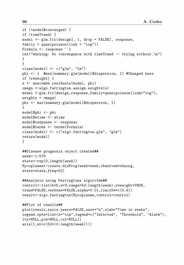
96 A. Codes
if (!model$converged) {
if (timeTrend) {
model <- glm.fit(design[, 1, drop = FALSE], response,
family = quasipoisson(link = "log"))
Formula <- response ~ 1
cat("Warning: No convergence with timeTrend -- trying without.\n")
}
}
class(model) <- c("glm", "lm")
phi <- 1 #max(summary.glm(model)$dispersion, 1) #Changed here
if (reweight) {
s <- anscombe.residuals(model, phi)
omega <-algo.farrington.assign.weights(s)
model <-glm.fit(design,response,family=quasipoisson(link="log"),
weights = omega)
phi <- max(summary.glm(model)$dispersion, 1)
}
model$phi <- phi
model$wtime <- wtime
model$response <- response
model$terms <- terms(Formula)
class(model) <- c("algo.farrington.glm", "glm")
return(model)
}
##Disease prognosis object created##
week<-1:578
state<-rep(0,length(week))
Mycoplasma<-create.disProg(week=week,observed=obsorg,
state=state,freq=52)
##Analysis using Farringtons algorithm##
control<-list(b=5,w=3,range=53:length(week),reweight=TRUE,
trend=FALSE,verbose=FALSE,alpha=0.01,limit54=c(5,4))
result<-algo.farrington(Mycoplasma,control=control)
##Plot of results##
plot(result,xaxis.years=FALSE,xaxt="n",xlab="Time in weeks",
legend.opts=list(x="top",legend=c("Infected", "Threshold", "Alarm"),
lty=NULL,pch=NULL,col=NULL))
axis(1,at=c(52*(0:length(week))))

A.3 The dynamic linear model 97
##Result tables##
beg<-145
end<-178
tableoutbreak.one<-data.frame(week=beg:end,
Infected=obsorg[(beg+52):(end+52)],
Threshold=result$upperbound[beg:end],
Alarm=result$alarm[beg:end])
View(tableoutbreak.one)
beg<-478
end<-490
tableoutbreak.two<-data.frame(week=beg:end,
Infected=obsorg[(beg+52):(end+52)],
Threshold=result$upperbound[beg:end],
Alarm=result$alarm[beg:end])
View(tableoutbreak.two)
A.3 The dynamic linear model
##Skewness correction##
obs<-obsorg^(2/3)
##Load of dlm package##
library(dlm)
##Function for estimation of unknown parameters##
build<-function(parm){
dlmModPoly(1, dV = exp(parm[1]), dW = exp(parm[2]))+
dlmModTrig(s = 52, q = 1, dV = 0,dW = exp(rep(parm[3],2)))
}
##Steady period for estimation of unknown parameters##
est<-obs[0:200]
est<-append(est,rep(NA,49),after=length(est))
est<-append(est,obs[250:500],after=length(est))
##Estimation of unknown parameters using MLE##
fit<-dlmMLE(est,rep(0,3),build)
##Model with estimated parameters##
model<-dlmModPoly(order=1,dV=exp(fit$par[1]),dW=exp(fit$par[2]))+
dlmModTrig(s=52,q=1,dV=0,dW=exp(rep(fit$par[3],2)))

98 A. Codes
##Kalman filter##
filter<-dlmFilter(est,model)
##The variances##
variance<-dlmSvd2var(filter$U.C,filter$D.C)
##The mean value of the prior##
model$m0<-apply(filter$m,2,mean)
##The variance of the prior##
model$C0<-variance[[125]]
##Analysis function##
OneStep<-function(X,lev=0.99){
L<-length(X$res)
if(L==length(X$y)) stop("The End")
f<-dlmFilter(X$y[L+1],X$mod)
fc <- dlmForecast(X$mod)
up<-(fc$f[1,1]+qnorm(lev)*sqrt(fc$Q[[1]][1,1]))^(3/2)
X$upper<-c(X$upper,up)
r<-(X$y[L+1]-fc$f[1,1])/sqrt(fc$Q[[1]][1,1])
if(r>qnorm(lev)){
X$res<-c(X$res,NA)
f<-dlmFilter(NA,X$mod)
}
else{
X$res<-c(X$res,r)
}
f<-dlmSmooth(f)
X$mod$m0<-f$s[2,]
X$mod$C0<-dlmSvd2var(f$U.S,f$D.S)[[2]]
X
}
##List containing the model and observations##
surv<-list(mod=model,y=obs,res=NULL)
##Analysis##
for(i in 1:length(obs)) surv<-OneStep(surv)
##Weeks with alarms##
ii<-(1:578)[is.na(surv$res)]

A.4 The multi-process dynamic linear model 99
##Plot of results##
plot(obsorg[53:578],type="h",main="",xaxt="n",xlab="Time in weeks",
ylab="No. infected")
axis(1,at=c(52*(0:length(obsorg))))
legend("top",c("Infected","Threshold","Alarm"),
lty=c(1,2,NA_integer_),pch=c(NA_integer_,NA_integer_,2),
col=c("black","blue","red"))
for(i in ii) points(c(i-52,i-52),c(-10,-10),col="red",pch=2)
lines(surv$upper[53:578],lty=2,col="blue")
##QQ-plot of the standard innovations##
qqnorm(surv$res,xlab="Normal Theoretical Quantiles")
abline(0,1)
##Tables with results##
Alarm<-is.na(surv$res)
beg<-145
end<-178
tableoutbreak.one<-data.frame(week=beg:end,
Infected=obsorg[(beg+52):(end+52)],
Threshold=surv$upper[(beg+52):(end+52)],
Alarm=Alarm[(beg+52):(end+52)])
View(tableoutbreak.one)
beg<-478
end<-490
tableoutbreak.two<-data.frame(week=beg:end,
Infected=obsorg[(beg+52):(end+52)],
Threshold=surv$upper[(beg+52):(end+52)],
Alarm=Alarm[(beg+52):(end+52)])
View(tableoutbreak.two)
A.4 The multi-process dynamic linear model
##Skewness correction##
obs<-obsorg^(2/3)
##Load of dlm package##
library(dlm)
##Function for estimation of unknown parameters##
build<-function(parm){
dlmModPoly(1, dV = exp(parm[1]), dW = exp(parm[2]))+
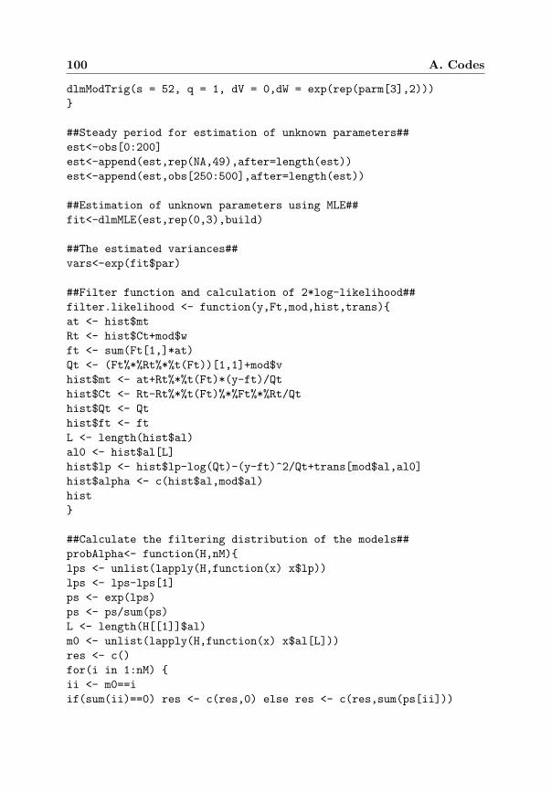
100 A. Codes
dlmModTrig(s = 52, q = 1, dV = 0,dW = exp(rep(parm[3],2)))
}
##Steady period for estimation of unknown parameters##
est<-obs[0:200]
est<-append(est,rep(NA,49),after=length(est))
est<-append(est,obs[250:500],after=length(est))
##Estimation of unknown parameters using MLE##
fit<-dlmMLE(est,rep(0,3),build)
##The estimated variances##
vars<-exp(fit$par)
##Filter function and calculation of 2*log-likelihood##
filter.likelihood <- function(y,Ft,mod,hist,trans){
at <- hist$mt
Rt <- hist$Ct+mod$w
ft <- sum(Ft[1,]*at)
Qt <- (Ft%*%Rt%*%t(Ft))[1,1]+mod$v
hist$mt <- at+Rt%*%t(Ft)*(y-ft)/Qt
hist$Ct <- Rt-Rt%*%t(Ft)%*%Ft%*%Rt/Qt
hist$Qt <- Qt
hist$ft <- ft
L <- length(hist$al)
al0 <- hist$al[L]
hist$lp <- hist$lp-log(Qt)-(y-ft)^2/Qt+trans[mod$al,al0]
hist$alpha <- c(hist$al,mod$al)
hist
}
##Calculate the filtering distribution of the models##
probAlpha<- function(H,nM){
lps <- unlist(lapply(H,function(x) x$lp))
lps <- lps-lps[1]
ps <- exp(lps)
ps <- ps/sum(ps)
L <- length(H[[1]]$al)
m0 <- unlist(lapply(H,function(x) x$al[L]))
res <- c()
for(i in 1:nM) {
ii <- m0==i
if(sum(ii)==0) res <- c(res,0) else res <- c(res,sum(ps[ii]))

A.4 The multi-process dynamic linear model 101
}
res
}
##The design matrix is defined##
Design <- model.matrix(~cos(2*pi*time*7/365)+sin(2*pi*time*7/365),
data=data.frame(time=1:length(obs)))
dimTheta <- dim(Design)[2]
##The variances##
vars <- c(vars,vars[3])
##The steady state model##
steady <- list(v=vars[1],w=diag(vars[-1]),al=1)
##The outlier model##
outlier <- steady
outlier$v=steady$v*10
outlier$al <- 2
##The outbreak model##
outbreak <- outlier
outbreak$al <- 3
##(2*log) The transition probabilities##
transition <- 2*log(matrix(c(.985,.01,.005,.985,.01,.005,
.09,.01,.9),3))
##The models##
models <- list(steady=steady,outlier=outlier,
outbreak=outbreak)
##The number of models##
numMod <- length(models)
##The history##
history <- list()
for(i in 1:numMod) history<-c(history,
list(list(lp=transition[i,1],
mt=rep(0,3),Ct=diag(rep(1,3)),alpha=i)))
##The lag##
lag<-3

102 A. Codes
##The number of models saved##
savenum <- numMod^(lag+1)
##Probability of each model##
alpha.probability <- c()
##Analysis##
for(i in 1:lag){
H <- list()
Ft <- matrix(Design[i,],1)
y <- obs[i]
for(mod in models){
for(hist in history)
H <- c(H,list(filter.likelihood(y,Ft,mod,hist,transition)))
}
history <- H
alpha.probability <- cbind(alpha.probability,
round(probAlpha(history,numMod),3))
}
for(i in (lag+1):length(obs)){
H <- list()
Ft <- matrix(Design[i,],1)
y <- obs[i]
for(mod in models){
for(hist in history)
H <- c(H,list(filter.likelihood(y,Ft,mod,hist,transition)))
}
lps <- unlist(lapply(H,function(x) x$lp))
history <- H[order(lps,decreasing=T)][1:savenum]
alpha.probability <- cbind(alpha.probability,
round(probAlpha(history,numMod),3))
}
##The most likely sequence of models##
pickMax<-function(x){
mx<-max(x)
ii<-(1:length(x))[x==mx]
min(ii)
}
mostLikely<-apply(alpha.probability,2,pickMax)
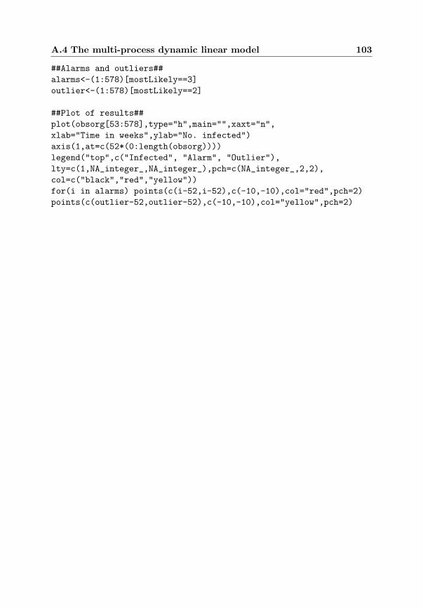
A.4 The multi-process dynamic linear model 103
##Alarms and outliers##
alarms<-(1:578)[mostLikely==3]
outlier<-(1:578)[mostLikely==2]
##Plot of results##
plot(obsorg[53:578],type="h",main="",xaxt="n",
xlab="Time in weeks",ylab="No. infected")
axis(1,at=c(52*(0:length(obsorg))))
legend("top",c("Infected", "Alarm", "Outlier"),
lty=c(1,NA_integer_,NA_integer_),pch=c(NA_integer_,2,2),
col=c("black","red","yellow"))
for(i in alarms) points(c(i-52,i-52),c(-10,-10),col="red",pch=2)
points(c(outlier-52,outlier-52),c(-10,-10),col="yellow",pch=2)