Detection and Impact of Industrial Subsidies: The

Case of World Shipbuilding

Myrto Kalouptsidi�y

Department of Economics, Princeton University and NBER

June 2015

Abstract

This paper provides a model-based empirical strategy to, (i) detect the pres-

ence and gauge the magnitude of government subsidies and (ii) quantify their

impact on production reallocation across countries, industry prices, costs and

consumer surplus. I construct and estimate an industry model that allows for

dynamic agents in both demand and supply and apply my strategy to world

shipbuilding, a classic target of industrial policy. I �nd strong evidence con-

sistent with China having intervened and reducing shipyard costs by 15-20%,

corresponding to 5 billion US dollars between 2006 and 2012. The subsidies

led to substantial reallocation of ship production across the world, with Japan,

in particular, losing signi�cant market share. They also misaligned costs and

production, while leading to minor surplus gains for shippers.

Keywords: industry dynamics, government subsidies, China, shipbuilding

�Princeton University, Department of Economics, 315 Fisher Hall, Princeton, NJ 08544-1021.email: myrto@princeton.edu

yI am very thankful to Jan De Loecker, Richard Rogerson, Eduardo Morales, as well as JohnAsker, Panle Jia Barwick, Allan Collard-Wexler and Eugenio Miravete for their helpful discussionsof the paper. The paper has also gained a lot from comments by Steve Berry, Chris Conlon, GeneGrossman, Bo Honore, Ariel Pakes, Paul Scott, Junichi Suzuki. Dan Goetz, as well as ConleighByers and Mengqin Chen provided excellent research assistance. Sarinka Parry-Jones and NatalieBurrows at Clarksons have been extremely helpful. Finally, I gratefully acknowledge the support ofthe National Science Foundation (under grant SES-1426933).

1 Introduction

In recent years, Chinese �rms have extremely rapidly dominated a number of capital

intensive industries, such as steel, auto parts, solar panels, shipbuilding.1 Government

subsidies are often evoked as a possible contributing factor to China�s expansion.2 Yet,

even though industrial subsidies have steered industrialization and growth in several

countries throughout economic history (e.g. in East Asia), little is known about

their quantitative impact on production reallocation across countries, industry prices,

costs and surplus. A signi�cant challenge in this task is that government subsidies

to industries are notoriously di¢ cult to detect and measure; and in China even more

so. Indeed, partly because international trade agreements prohibit direct and in-kind

subsidies, �systematic data are non-existent�3 and thus the presence and magnitude

of such subsidies is often unknown.

This paper assesses the consequences of government subsidies on industrial evo-

lution, focusing on the unparalleled and timely Chinese expansion. Since measuring

subsidies is a prerequisite for this analysis, I provide a model-based empirical strategy

to detect their presence and gauge their magnitude. I apply my empirical strategy to

the world shipbuilding industry, a classic target of industrial policy. In 2006, China

identi�ed shipbuilding as a �strategic industry�and introduced a plan for its develop-

ment.4 Within a short time span, its market share doubled from 25% to 50%, leaving

Japan, S. Korea and Europe trailing behind. Many asserted that China�s rapid rise

was driven by hidden government subsidies that reduced shipyard production costs,

as well as by a number of new shipyards constructed through the government plan;

here I assess the relative contribution of these interventions.

I develop and estimate a model of the shipbuilding industry, providing one of

the �rst empirical analysis in industrial organization looking at dynamic agents on

both the demand and the supply side. A large number of shipyards o¤er durable,

1The share of labor intensive products in Chinese exports fell from 37% to 14% between 2000and 2010. On a monthly basis, in 2011 the US imported advanced-technology products from China560% more than it exported to China. By contrast, the monthly US-China trade surplus in scrap(used as raw material) grew by 1187% between 2000 and 2010. (U.S.-China Economic and SecurityReview Commission (2011)).

2�China is the workshop to the world. It is the global economy�s most formidable exporter and itslargest manufacturer. The explanations for its success [include the] seemingly endless supply of cheaplabour (...) another reason for China�s industrial dominance: subsidies.�(�Perverse Advantage�, TheEconomist, April 2013).

3WTO (2006).4Section 2 provides details.

1

di¤erentiated ships. Their production decisions are subject to a dynamic feedback

because of time to build: shipyards accumulate backlogs, which a¤ect their future

ability to accept new ship orders. Production cost is also subject to an aggregate

stochastic shock, summarized in the price of steel, a key production input. Every

period a large number of identical potential shipowners decide to enter the freight

market by buying a new ship from world shipyards. Demand for new ships is driven

by demand for international sea transport, which is uncertain and volatile. As ships

are long-lived investments for shipowners, demand for new ships is dynamic.

The model primitive of interest is the cost function of potentially subsidized �rms.

As in many industries, however, costs of production are not observed. My strat-

egy amounts to estimating costs from demand variation in a framework of dynamic

demand and supply. In the simplest example of a static, perfectly competitive frame-

work, marginal cost is recovered directly from prices. In that case, the detection

strategy amounts to testing for a break in observed ship prices when China launched

its shipbuilding plan. In my setup, there are two complications: (i) new ship price

data are scant, and (ii) the shipbuilding production decision is subject to dynamic

feedbacks. To address (i), I add used ship prices; to address (ii) I use the shipyard�s

optimality conditions resulting from its dynamic optimization.

My estimation strategy can be summarized as follows. To estimate shipyard costs,

I adopt a novel approach that is inspired by the literature on estimation of dynamic

setups, e.g. Hotz and Miller (1993), Bajari, Benkard and Levin (2007) and Pakes, Os-

trovsky and Berry (2008), as well as Xu (2008), Ryan (2012), Collard-Wexler (2013)

and others: I �rst invert observed choice probabilities to obtain directly the optimal

policy thresholds nonparametrically in an ordered-choice dynamic problem; I then

show that the latter lead to a closed-form expression for ex ante optimal per period

payo¤s, which in turn are su¢ cient to obtain shipyard value functions. To recover de-

mand for new ships I estimate the willingness to pay using new and used ship prices,

as well as shipowner expectations (similar to Kalouptsidi (2014)). The estimation

allows expectations and value functions to be di¤erent before and after 2006, con-

sistent with China�s intervention. Finally, in estimating dynamics, I employ sparse

approximation techniques (LASSO) that allow for a very large state space, as well as

signi�cant �exibility. Solving value functions via LASSO, which to my knowledge has

not be used before, can be very useful to other applications with dynamic agents and

a large state space.

2

I use my framework to detect and measure changes in costs that are consistent with

subsidies. I �nd a strong signi�cant decline in Chinese costs, consistent with subsidies

equal to about 15-20% of costs, or 5 billion US dollars at the observed production

levels. A concern may be that this decline is not driven by subsidies, but rather by

technological change, or learning-by-doing. To address this concern, I perform several

robustness checks. I �nd that the results are robust to many speci�cations that control

�exibly for time-variation. I also provide evidence that costs did not change in other

countries. Most convincingly, the results hold when I estimate costs on the subset

of shipyards that existed prior to 2001. These shipyards are no longer learning-by-

doing, nor did their technology change (bulk ship production is not characterized by

technological innovations to begin with).

Next, I use my framework to quantify the contribution of government interven-

tions in China�s seizing of the market. My main counterfactual predicts industry

evolution (production reallocation across countries, ship prices, industry costs and

shipper surplus) in the absence of China�s government plan altogether; note that

both cost subsidies and new shipbuilding facilities would violate international trade

agreements. Moreover, I assess the relative contribution of the new shipbuilding facili-

ties constructed through China�s plan in a second counterfactual that removes the new

facilities, but maintains the cost subsidies detected above. Here is a brief summary

of my main four �ndings from these counterfactuals.

First, I �nd that the interventions led to substantial reallocation in production: in

the absence of China�s government plan, its market share is cut to half, while Japan�s

share increases by 50%. If only new shipyards are removed, China�s share falls from

50% to 40%, suggesting that they played an important, but not the predominant

part in China�s expansion. The dynamic feedback in production, captured by the

dependence of costs on backlog, is responsible for about 7% of this reallocation.

Second, ship prices experience moderate increases in all countries in the absence

of China�s plan, as the latter shifted supply outward.

Third, freight rates decrease moderately because of the larger �eet between 2006

and 2012 and more so over time due to time to build, compared to a world without

China�s intervention. As a result of China�s plan, cargo shippers gain about 290

million US dollars in shipper surplus over that time period. Comparing this gain to

the 5 billion US dollars of cost subsidies alone implies that the bene�ts of subsidies

within the maritime industries are minimal and perhaps the Chinese government is

3

aspiring to externalities to di¤erent sectors (e.g. steel, defense).

Fourth, subsidies create a wedge in the alignment of market share and production

costs: they lead to a large increase in the industry average cost of production (net

of subsidies) by shifting production away from low-cost Japanese shipyards towards

high-cost Chinese shipyards.

This paper contributes to the recent empirical literature on industry dynamics (e.g.

Benkard (2004), Aguirregabiria and Mira (2007), Xu (2008), Ryan (2012), Collard-

Wexler (2013)). Methodologically, it lies closest to Hotz and Miller (1993), Bajari,

Benkard and Levin (2007) and Pakes, Ostrovsky and Berry (2007). This literature

typically considers either single agent dynamics or dynamic �rms and static consumers

(one exception is Chen, Esteban and Shum (2013)). In contrast, this paper allows

for dynamics in both demand and supply; these dynamics are important in many

durable goods markets (e.g. autos, TV�s), as well as upstream-downstream industries

(e.g. airlines-aircraft builders, shipping-shipbuilders). In Kalouptsidi (2014) I focus

only on the downstream industry of shipping. Here, I focus on the upstream industry

of shipbuilders, modeling their demand (shipping) similarly to Kalouptsidi (2014).

The paper also naturally contributes to the literature on trade policies. Goldberg

(1995) and Berry, Levinsohn and Pakes (1999) consider the impact of voluntary export

restraints in the automobile industry. Grossman (1990) provides an excellent survey

of the relevant trade literature, while Brander (1995) is a classic reference on the long

theoretical literature of strategic trade (see also references within). Not surprisingly,

given the constraints in subsidy data availability, there is little empirical work, most

of which is in the form of model calibration. Baldwin and Krugman (1987a) and

(1987b) explore the impact of trade policies in the wide-bodied jet aircraft and the

semiconductor industries, while Baldwin and Flam (1989) in the small commuter

aircraft industry. They all discuss the lack of knowledge regarding both the presence

and magnitude of subsidies and other policies and compute industrial evolution under

di¤erent hypothetical scenarios.

The remainder of the paper is organized as follows: Section 2 provides a descrip-

tion of the environment under study including subsidy regulations and features of

the industry. Section 3 presents the model. Section 4 describes the data used and

provides some descriptive evidence. Section 5 presents the empirical strategy and the

estimation results. Section 6 provides the counterfactual experiments and Section 7

concludes.

4

2 Environment

Subsidy Disputes Subsidy disputes are handled both bilaterally (e.g. in the US

the relevant agencies are the Department of Commerce and the International Trade

Commission (ITC)), as well as internationally through the WTO. They often lead to

retaliating measures (countervailing measures or subsidy wars), which may spiral the

e¤ects of the original subsidies and further the reallocation.5 Deciding on subsidy

complaints is di¢ cult for two reasons; �rst, �systematic data (on industrial subsidies)

are non-existent; reliable sources of information are scarce and mostly incomplete [...]

because governments do not systematically provide the information�(WTO (2006)).

Therefore, detecting and measuring subsidies becomes a di¢ cult task and plainti¤s

need to base their allegations mostly on available self-reported data.6 The second

di¢ culty concerns (dis)proving �injury caused�by the alleged subsidies.7 Ideally, the

question to be answered is �how would have this industry evolved absent the alleged

subsidies?�; this is clearly a di¢ cult question which is answered based on a mostly

qualitative analysis of industry indicators on a case by case basis.

China has had more trade con�icts than any other country in the world, in more

industries and with more countries.8 China provides industry subsidies in the form

of free or low-cost loans, as well as subsidies for inputs (including energy), land and

technology. Because of institutional and strategic reasons, the information on sub-

sidies that the Chinese government provides has rampant missing and misreported

5�The ITC received a total of 1,606 antidumping and countervailing duty petitions during 1980-2007. These cases involved over $65 billion in imports. Thirty-eight percent of the petitions resultedin a¢ rmative determinations by the Commission and Commerce, culminating in the issuance of anantidumping or countervailing duty order.�(ITC (2008))

6One possible source of information (other than e.g. national accounts or individual governmentmeasures (Sykes (2009))) are subsidy �noti�cations�required by the WTO under SCM; however �thedata contain many gaps and shortcomings. Not all Members ful�ll the noti�cation requirements. 29of the currently 149 WTO Members have so far not submitted any noti�cation. [...] Other Membersdo not provide quantitative information on subsidy programmes or do not provide this informationsystematically. In most years, information is available for less than half of the WTO membership.�(WTO (2006))

7For example, in the US �an interested party may �le a petition with ITC and Commerce allegingthat an industry in the United States is materially injured or threatened with material injury, orthat the establishment of an industry is materially retarded, by reason of imports that are beingsubsidized�(ITC (2008)). �Material injury�amounts to observing the volume of imports, as well astheir impact on the domestic industry�s prices and production. WTO�s SCM has similar provisions:complaining countries must provide evidence of adverse trade e¤ects in their own or third countrymarkets (as well as evidence on the existence and nature of subsidies as mentioned above).

8The rest of the section draws from Haley and Haley (2008).

5

data.9 These subsidies are often transferred through �nancial institutions, most of

which are directed by the central and provincial governments.

Shipbuilding and China�s Plan10 Shipbuilding is one of the major recipients of

subsidies globally, along with e.g. the steel, mining and automotive industries. It is

often seen as a �strategic industry� as it increases industrial and defence capacity,

generates employment and has important spill-overs to other industries (e.g. iron

and steel). Indeed, several of today�s leading economies developed their production

technologies and human capital through a phase of heavy industrialization, in which

shipbuilding was one of key pillars. In the 1850�s, Britain was the world leading

shipbuilder, until it was overtaken by Japan in the 1950�s, which in turn lost its

leading position to Korea, in the 1970�s (4:5% of its GDP today).

China�s 11th National 5-year Economic Plan 2006-2010 was the �rst to appoint

shipbuilding as a �strategic industry�in need of �special oversight and support�; the

central government �unveiled an o¢ cial shipbuilding blueprint to guide the medium

and long-term development of the industry�. As part of the national plan, the cen-

tral government introduced the �Medium and Long-Term Plan for the Shipbuilding

Industry� ( ) 11 which expands capacity and provides �nancial

support for output growth (cheap credit, low input prices, etc.).

The majority of Chinese shipbuilding production occurs at (i) a number of ship-

yards under the umbrella of two major state-owned enterprises directly administered

by the Chinese central government (CSSC and CSIC); (ii) numerous shipyards ad-

ministered by provincial and local governments. Moreover, China�s shipbuilding is

mostly geared towards export sales which comprised about 80% of its production in

2006.

Consistent with the above mentioned government programs, Figure 1 shows China�s

rapid expansion in shipbuilding dry docks, the majority of which (82%) was realized

through the construction of new facilities. In contrast to the capital expansion, which

9In its 2014 report the US-China Economic and Security Commission (a US government bodyestablished to monitor and investigate national security implications of the bilateral trade and eco-nomic relationship between the United States and China) states that �a full identi�cation of supportprogrammes was not possible for the Secretariat, as they are often the result of internal adminis-trative measures that are not always easy to identify and generally only available in Chinese. Inaddition, the budget is not a public document hence it is not possible to identify outlays.�10This section draws from OECD (2008), Collins and Grubb (2008) and Stopford (2009).11The plan was introduced by the National Development and Reform Commission (NDRC) and

the Commission of Science, Technology and Industry for National Defence (COSTIND).

6

is observed, subsidies that reduce operating costs are not observed. The two mea-

sures also di¤er in their implementation. Entry/Capital expansion decisions are not

taken at the shipyard level, but rather at the higher administrative level (i.e. CSSC,

CSIC, regional governments). Indeed, a signi�cant portion of CSSC and CSIC �nan-

cial resources have been devoted to expanding China�s shipbuilding infrastructure.12

In contrast, the day-to-day operations and contract bids are handled directly by the

individual shipyards. This distinction is taken into account in the model and is dis-

cussed further in Sections 3 and 5. Finally, it is important to note that both types

of interventions would violate trade agreements; the relevant question of interest to

disciplining authorities is how the industry would evolve in the absence of all measures.

Figure 1: Shipbuilding dry docks.

Commercial ships are the largest factory produced product. Materials account for

about half the cost of the ship (steel is about 13%) and labor (mostly low skill tasks)

about 17% of total cost. This paper focuses on cargo transportation and in particular,

dry bulk shipping, which concerns vessels designed to carry a homogeneous unpacked

cargo (mostly raw materials), for individual shippers on non-scheduled routes. The

bulk shipping market consists of a large number of small shipowning �rms (largest

�rm has share 3%).13

3 Model

In this section, I present a dynamic model for world shipbuilders, following the tradi-

tion of Hopenhayn (1992) and Ericson and Pakes (1995). A key input is demand for

new ships, which stems from the decisions of downstream shipowners to purchase new

12As an example, �CSSC had multibillion-dollar projects under way to build new shipyards onChangxing Island in Shanghai and Longxue Island in Guangzhou�.13See Kalouptsidi (2014) for a detailed description of the bulk shipping industry.

7

vessels. I therefore begin this section by describing shipowner behavior. Next, I turn

to upstream shipbuilder behavior, which is the focus of this paper. I also discuss how

government subsidies enter. Variables with superscript �o�refer to shipowners and

�y�to yards, while subscripts i and j refer to a particular owner and yard respectively.

In the model, shipyards do not make entry or capital expansion decisions: as

discussed above, in China these decisions are not made by individual shipyards, but

rather by the central government through either the state conglomerates, or regional

authorities. Moreover, no signi�cant changes in docks are observed in other countries;

see Figure 1. I discuss this further in the estimation results.

3.1 Demand for New Ships (Shipowners)

Time is discrete and the horizon is in�nite. There is a �nite number of incumbent

shipowners (the �eet) and a large number of identical potential entrant shipowners.

I assume constant returns to scale, so that a shipowner is indistinguishable from his

ship. Ships are long-lived. The state variable of ship i at time t, soit, includes its:

1. age 2 f0; 1; :::; Ag

2. country where built 2 C

while the industry state, st, includes the:

1. distribution of characteristics in soit over the �eet, sot 2 RA�jjCjj

2. backlog bt 2 RJ�T , whose (j; k)th element is the number of ships scheduled tobe delivered at t+ k by shipyard j = 1; :::; J and T the maximum time to build

3. aggregate demand for shipping services, dt 2 R+

4. price of steel, lt 2 R+.14

In period t, each shipowner i chooses how much transportation (i.e. voyages

travelled) to o¤er, qoit. Shipowners face the inverse demand curve:

Pt = P (dt; Qot ) (1)

14The steel price is part of the state because it: (i) is a key determinant of shipyard productioncosts; (ii) determines the ship�s scrap value.

8

where Pt is the price per voyage, dt de�ned above includes demand shifters, such as

world industrial production and commodity prices and Qot denotes the total voyages

o¤ered, so that Qot =P

i qoit. Voyages are a homogeneous good, but shipowners face

heterogeneous convex costs of freight. Ship operating costs increase with the ship�s

age and may di¤er based on country of built because of varying quality.

I assume that shipowners act as price-takers in the market for freight. Their

resulting per period payo¤s are �o (soit; st).15

A ship lives a maximum of A periods. At the same time, a ship can be hit by

an exit shock each period.16 In particular, I assume that a ship at state (soit; st) exits

with probability � (soit; st) and receives a deterministic scrap value � (soit; st). Note that

ships exit with certainty at age A.17

The only dynamic control of shipowners is entry in the industry: each period,

a large number of identical potential entrants simultaneously make entry decisions.

There is time to build, in other words, a shipowner begins its operation a number

of periods after its entry decision. To enter, shipowners purchase new vessels from

world shipyards. Shipyard j in period t can build a new ship at price PNBjt and time

to build Tjt. The assumption of a large number of homogeneous potential shipowners

implies that shipyard prices are bid up to the ships�values and shipyards can extract

all surplus. One can also think of this as a free entry condition in the shipping

industry where the entry cost is equal to the shipyard price. Therefore, the following

equilibrium condition holds:

PNBjt = Eh�TjtV o

�soit+Tjt ; st+Tjt

�jsoit; st

i(2)

where � is the discount factor and soit in this case involves ship age equal to zero

and the country of yard j, while the value function V o (soit; st) satis�es the Bellman

equation:

V o (soit; st) = �o(soit; st) + �(s

oit; st)�(s

oit; st) + (1� �(soit; st))�E

�V o�soit+1; st+1

�jsoit; st

�(3)

15More accurately, ship pro�ts from freight are �o�soit; s

ot ; dt

�; even though the backlog and steel

prices do not a¤ect current payo¤s, they a¤ect state transitions and scrap values and are thus partof the state.16Shipowners scrap their ships by selling them to scrapyards where they are dismantled and their

steel hull is recycled.17Generalizing to endogenous exit is straightforward (see Kalouptsidi (2014)).

9

In words, the value function of a ship at state (soit; st) equals the pro�ts from cargo

transport plus the scrap value which is received with probability �(soit; st) and the

continuation value E�V o�soit+1; st+1

�jsoit; st

�, which is received with probability 1 �

�(soit; st).

In practice, shipowners can also buy a used ship. In this model, since ships are

indistinguishable from their owners, transactions in the second-hand market do not

a¤ect entry or pro�ts in the industry. In addition, since there is a large number of

identical shipowners who share the value of a ship, the price of a ship in the second

hand market, P SHit , equals this value and shipowners are always indi¤erent between

selling their ship and operating it themselves. Therefore, in equilibrium:

P SHit = V o (soit; st) (4)

I revisit sales in the empirical part of the paper, where both second-hand prices are

treated as observations on the value function.

3.2 Supply of New Ships (Shipyards)

There are J long-lived incumbent shipbuilders. The state variable of shipyard j at

time t, syjt, includes its:

1. backlog bjt 2 RT

2. country

3. other characteristics, such as: age, capital equipment (number of docks and

berths, length of largest dock), number of employees.

Shipyards also share the industry state, st.

In period t, shipyard j draws a private iid (across j and t) production cost shock

"jt, with �"jt � N (0; 1), and makes a discrete production decision qjt 2 f0; 1; :::; qg.18

Shipyard j faces production costs, C�qjt; s

yjt; st; "jt

�. Even though qjt is an integer I

assume that the cost function can be de�ned over the real interval [0; q] and that as

such it is convex in qjt. I also assume that the cost shock "jt is paid for each produced

18Allowing for serially correlated unobserved state variables is a di¢ cult issue that the literaturehas not yet tackled.

10

unit, so that:

C�qjt; s

yjt; st; "jt

�= c

�qjt; s

yjt; st

�+ �qjt"jt (5)

In this model qjt corresponds to the number of ships ordered in period t at shipyard

j. These ships enter the shipyard�s backlog bjt and are delivered a number of years

later.19 Under demand uncertainty, therefore, undertaking a ship order becomes a

dynamic choice. To capture this dynamic feedback, I assume that the cost function

depends on the shipyard�s backlog. As in Jofre-Bonet and Pesendorfer (2003), there

are two opposing ways the backlog can impact costs: on one hand, increased backlogs

can raise costs because of capacity constraints (e.g. less available labor); on the other

hand, increased backlogs can lower costs because of economies of scale (e.g. in ordering

inputs) or the accumulation of expertise.20

As discussed above, shipyard j sells its ships at a price equal to the shipowners�

entry value:21

V Eoj (st) � Eh�TjtV o

�soit+Tjt;st+Tjt

�jsoit; st

i(6)

where soit+Tjt has zero ship age and the country of yard j. Time to build is shipyard-

speci�c and in particular, Tjt = T�syjt; st

�. Note that V Eoj (st) does not explicitly

depend on period t�s production, qjt; in other words yards do not face a downward

sloping demand curve. Indeed, qjt a¤ects the willingness to pay for the ship by entering

into the total backlog bt and from there into the �eet after Tjt periods. Typically, qjtis a small integer, while the total �eet is a large number in the order of thousands.

Therefore each shipyard, when making its production decision, can ignore the impact

it has on V Eoj (st); note however, that aggregates do matter so that as the total �eet

increases, shipowners�willingness to pay falls, all else equal.

Shipyard j chooses its production level to solve the Bellman equation:

19I consider the number of orders as the relevant choice variable (as opposed to using the numberof deliveries or smoothing orders) because the observed ship prices are paid at the order date andmay be dramatically di¤erent from the prevailing prices at the delivery date.20Here, the shipyard�s backlog also a¤ects its demand, as it increases the time shipowners have to

wait for delivery.21Note that the willingness to pay for a new ship from yard j depends only on its country of origin,

not j itself. Even though it is straightforward in the model to allow a ship�s value to change withj, the hundreds of shipyards encountered in the data make this generalization impossible in thisempirical application.

11

V y�syjt; st; "jt

�= max

0�q�qV Eoj (st) q�c

�q; syjt; st

���q"jt+�E

�V y�syjt+1; st+1; "jt+1

�jsyjt; st; q

�(7)

To ease notation, I also de�ne the continuation value:

CV y�syjt; st; q

�� E

�V y�syjt+1; st+1; "jt+1

�jsyjt; st; q

�(8)

The expectation in (7), as well as in ship value functions (2) and (3), is over demand

for shipping services, dt, steel prices, lt, shipyard production qjt, all j and j�s future

cost shocks. The demand state variable dt and steel prices lt evolve according to a

�rst order autoregressive process with trend (see Section 5:1:1). Period t production,

qjt, enters j�s backlog, bjt, at position Tjt, while the remaining elements of bjt move

one period closer to delivery with its �rst element being delivered. The evolution of

all other states is deterministic (see Section 5:1:1). The trend component in demand

and steel prices implies that time t is explicitly part of the state (in other words,

the state notation�soit; s

yjt; st

incorporates t). Allowing for time to enter the agents�

decision-making o¤ers some generality and is important in this application, as my

empirical analysis of detecting government subsidies hinges on allowing time-varying

factors to a¤ect costs.

Under convex costs, the shipyard�s optimal policy amounts to comparing each

production level q to q + 1 and q � 1, as stated in the following intuitive lemma:

Lemma 1 If the shipbuilding cost function C (q; �) : [0; q] ! R, is convex in q, thenthe shipyard�s optimal policy is given by:

q��syjt; st; "jt

�=

8>>>>>>><>>>>>>>:

0; if "jt � A�syjt; st; 0

�q; if "jt 2

hA�syjt; st; q � 1

�; A�syjt; st; q

� iq; if "jt � A

�syjt; st; q � 1

�(9)

12

where

A�syjt; st; q

�� 1

�

264 V Eoj (st) +

�c�q; syjt; st

�� c

�q + 1; syjt; st

��+

+��CV y

�syjt; st; q + 1

�� CV y

�syjt; st; q

��375

for q = 0; 1; :::; q � 1, are the optimal policy thresholds.

Proof. See the Online Appendix.The timing in each period is as follows: incumbent and potential entrant shipown-

ers observe their state (soit; st), while shipbuilders observe their state�syjt; st

�. Shipown-

ers are hit by exit shocks and shipbuilders observe their private production cost shocks.

Shipyards make production decisions. Next, shipowners receive pro�ts from freight

services and shipyards receive pro�ts from new ship production. Exiting ships receive

their scrap value �(soit; st). Finally, states are updated.

I consider a competitive equilibrium which consists of an optimal production policy

function q��syjt; st; "jt

�that is given by (9), as well as value functions V y

�syjt; st

�and V o (soit; st) that satisfy (7) and (3) respectively, while all expectations employ

q��syjt; st; "jt

�. Existence of equilibrium follows from Doraszelski and Satterthwaite

(2010), Hopenhayn (1992), and Jovanovic (1982).

Finally, I assume that China�s plan was an unexpected, one-shot, permanent and

immediate change from the point of view of industry participants. Explicitly modeling

expectations with regard to policy interventions is extremely complicated and would

rely on strong and undoubtedly ad hoc assumptions. Within my model, the before and

after 2006 worlds di¤er in the set of shipyards, China�s cost function and shipbuilding

infrastructure (found in syjt).

4 Data and Descriptive Evidence

Data All data I use come from Clarksons. I employ �ve di¤erent datasets. The

�rst, reports shipbuilding quarterly production (i.e. orders) between Q1-2001 and

Q3-2012. For each shipyard and quarter I observe its bulk ship production in tons

and numbers, as well as the yard�s backlog and average time to build. There are 192

yards that produce Handysize vessels (the segment on which my empirical analysis

will focus), of which 119 are Chinese, 41 are Japanese, 21 are S. Korean and 11 are

13

European. The majority of bulk ship production occurs in China and Japan; hence

even though I include Europe and S. Korea in the estimation and counterfactuals,

most comparisons will be made between China and Japan.

The second dataset is a sample of shipbuilding contracts, between August 1998

and August 2012. It reports the order and delivery dates, the shipyard and price in

million US dollars. Unfortunately, prices are reported for only a fraction of contracts.

I illustrate this in Figure 2, which plots the average reported new ship price per

country and quarter. Note that several quarters, especially in the pre-2006 period

involve missing prices. In addition, for shipyard-quarter combinations that involve

zero production, the corresponding price does not exist by default.

Figure 2: Average quarterly new ship price.

To deal with these issues, I introduce a dataset of second-hand ship sale transac-

tions, between August 1998 and August 2012. The dataset reports the date of the

transaction, the name and age of the ship, as well as the price in million US dol-

lars. I end up with 418 observations of new ship contracts and 2016 observations

of second-hand sale contracts (2434 total), of which 1173 are pre-2006 and 1261 are

post-2006.

The fourth dataset employed is a snapshot of shipyard characteristics in 2012, such

as shipyards��rst year of delivery, location, number of dry docks and berths, length of

largest dock, number of employees, total past output. Several shipyards have missing

observations. The �rst year of delivery is used to compute the shipyard�s age.22 The

number of docks and berths is a measure of capacity, since production bottlenecks

occur during the assembly operations done on the docks/berths. I allow the capital

22Because of time to build, I subtract a number of years from every �rst delivery year of allshipyards, after consulting with Clarksons�analysts. The results I report subtract 3 years (similar�ndings were obtained when I vary the number of years subtracted).

14

infrastructure of yards (i.e. docks/berths and length) to be di¤erent before and after

China�s plan by collecting data from a Clarksons publication (�World Shipyard Mon-

itor�). The adoption of a pre- and post-2006 capital infrastructure level is consistent

with the modeling assumption of two equilibria before and after China�s plan. I drop

shipyards with missing capital measures (docks/berths) so that the end shipyard sam-

ple (production and characteristics) consists of 4741 shipyard-quarter observations (all

results are robust if the full sample is used).

Finally, the �fth dataset consists of quarterly time-series between 1998 and 2012

for the �eet, total backlog, orders of new ships, deliveries, demolitions between 1998

and 2012. This dataset is used to create the states and estimate their transition. I

also obtain quarterly time-series of Japan�s steel ship plate commodity price in dollars

per ton during the same time period.23

Descriptive Evidence What patterns of the raw data are consistent with the

presence of subsidies? One might expect that new ship prices should react around

2006. As Figure 2 shows, the sparsity of new ship prices makes it impossible to explore

this. Used ship prices, however, should also display a reaction. I, therefore, run a

hedonic regression of second hand prices on ship characteristics (age and country

where built) and quarter dummies. Figure 3 shows that indeed there is a short-lived

drop in 2006, in a period when ship prices are trending upward due to increased

demand for freight (shifts in demand are also the reason the price decline is not

permanent in the raw data).24 Of course, this �nding is not proof of cost subsidies;

yet if no drop were observed, one may have been concerned about the impact of this

policy.

Despite the importance of a price response, the main insight of this paper, in terms

of identifying/measuring subsidies, is that production patterns are equally important.

Figure 4 depicts the evolution of China�s market share. Between 2005 and 2006,

China experiences a large, rapid increase in market share. In this paper, I employ

precisely this rapid increase in production (in combination with prices) to identify

changes in costs that are consistent with the presence of subsidies. At the same time,

the constructed model can control for the di¤erent factors leading to this increase

and provide a measurement of the alleged subsidies, a fundamental input into subsidy

23Due to space limitations, some summary statistics are reported in the Online Appendix.24I have unsuccessfully searched extensively in industry publications for alternative explanations.

15

Figure 3: Hedonic regression of used ship prices on ship age, country and quarterdummies.

disputes. When I come to the results, I discuss alternative explanations for this

pattern (e.g. productivity changes/technological improvements or learning by doing)

and argue that they cannot account for the observed patterns.

Figure 4: China�s market share.

5 Model Estimation and Detection of Subsidies

To see the main idea behind the subsidy detection method, consider a static, perfectly

competitive market, so that PNBjt = MCjt for all j and t. In that case, to detect

subsidies one would simply look for a break in observed prices in 2006, since prices

are in fact the marginal costs. In my setup, there are two complications: (i) I do

not observe enough prices of new ships, and (ii) there are dynamics in the production

decision. To address (i), I complement with used ship prices; to address (ii) I use the

shipyard�s �rst order condition from its dynamic optimization.

The proposed strategy proceeds in two steps. In the �rst step, I recover the

demand curve that shipbuilders face, which coincides with the value that shipowners

place on entering the shipping industry. Retrieving this willingness to pay for a new

16

ship amounts to estimating the value function for a new ship, as well as shipowner

expectations. The second step inserts the estimated willingness to pay for a ship into

the optimization problem of shipbuilders to recover their costs.

Each estimation task is described below and followed by the results. A time pe-

riod is a quarter. All results presented are for bulk vessels, in particular, Handysize.

There are three good reasons to focus on bulk carriers: China was already an impor-

tant player before 2006; their production process is not characterized by signi�cant

technological advances; product di¤erentiation is limited.25

5.1 Estimation of the Willingness to Pay for a New Ship

In this step, I estimate ship value functions and state transitions. All ship states

are directly observed in the data except for the demand for shipping services, dt. I

construct dt following Kalouptsidi (2014) by estimating a demand curve for shipping

services and using the intercept. The analysis is presented in the Appendix.

5.1.1 State Transitions

In order to compute the value of entering the shipping industry, de�ned in (6), I

need shipowner expectations over (soit; st). The transition of soit is known (age evolves

deterministically, while country of built is time invariant). The transition of st is

computationally complex: on one hand the dimension of the state space is enormous

(sot has dimension 4�A -whereA is a ship�s maximum age- in the case of four countries,while the backlog bt has dimension J � T which in my sample is in the order of

several thousand); on the other hand, updating bt requires optimal production policies

for all shipyards. Instead of working with the true transitions (as in Kalouptsidi

(2014)) I follow Jia Barwick and Pathak (2012) who assume that st follows a vector

autoregressive (VAR) model; this is similar to the �rst step of two-step estimation

procedures for dynamic games (e.g. Bajari, Benkard and Levin (2007) and Pakes,

Ostrovsky and Berry (2007)).

To deal with the state dimension, I make the following simplifying assumptions.

First, I replace the �eet distribution, sot , with two age groups�so1t; s

o2t

�: the number of

25Looking at other ship types (and even di¤erent aggregations across types) reveals that virtuallyall experience the same market evolution, with China displacing other countries (e.g. Figure 4 isvery similar across types); therefore concerns that perhaps countries started specializing in di¤erentships are put to rest.

17

ships below 20 years old and the number of ships above 20 years old.26 I do not use

the distribution of the �eet over country of built because its evolution is extremely

slow. Second, I replace the backlog, bt, with the total backlog Bt =P

j;l bjtl.27

I have experimented with several variations of the general time varying vector

autoregression (VAR) model:

st = Rot +Rtst�1 + �t

where �t � N (0;��). I allow the VAR parameters (Rot; Rt) to be di¤erent before

and after 2006: since state transitions are not modeled explicitly, the VAR model

embraces equilibrium features of agents�expectations that are likely to change after

China�s intervention. In particular, shipowners are likely to believe that all else equal

the supply of ships is permanently higher post 2006. This change a¤ects their ship

valuations today and therefore captures any changes in demand for new ships, brought

by China�s policies. I consider Q3-2005 as the �rst quarter of the post world (for all

empirical tasks in the paper), consistent with Figures 1 and 3; all results are robust

to alternative thresholds around that date.

I examined several speci�cations where (Rot; Rt) vary deterministically (e.g. time

trend, so that Rot = Ro + R� t) or randomly with time (random walk model for Rtdetermined by the Kalman �lter), or are time-invariant; end results are very robust.

The baseline speci�cation is:

26666664so1t

so2t

Bt

dt

lt

37777775 =26666664rs1o

rs2o

rBo

rd0

rl0

37777775 1 ft � 2006g+26666664rs10o

rs20o

rB0o

rdo

rlo

37777775 1 ft > 2006g+266666640

0

0

rd�

rl�

37777775 t+26666664rs1s1 rs1s2 rs1B rs1d rs1l

rs2s1 rs2s2 rs2B rs2d rs2l

rBs1 rBs2 rBB rBd rBl

0 0 0 rd 0

0 0 0 0 rl

37777775 st�1+�t(10)

and �� is diagonal and I work with natural logarithms for�so1t; s

o2t; Bt

�. Note that

as discussed above, demand dt and steel price lt are exogenous to the model and

are una¤ected by the pre/post-2006 regime. In contrast, I allow�so1t; s

o2t; Bt

�to be

26I have also worked with statistics of the �eet age distribution (total �eet, mean age, variance ofage) and found the results to be robust.27Ideally, the distribution of shipyards over their characteristics syjt would also be part of the state;

it is omitted for computational tractability.

18

a¤ected by all variables to account for ship entry and exit. The baseline speci�cation

allows only R0 to change before and after 2006. Even though t appears explicitly

only in the exogenous variables, it a¤ects�so1t; s

o2t; Bt

�through their dependence on

(dt; lt). I estimate the parameters of interest (R0; R;��) via OLS separately for each

variable (note that separate OLS yields identical estimates to Maximum Likelihood

estimation). Table 1 reports the results. All variables are persistent. Signs are also

in general as expected: so1t is increasing in the backlog and demand and decreasing in

steel prices (as steel prices increase, exit increases); so2t is decreasing in so1t, as more

young ships increase exit, and also so2t is increasing in demand which leads to less exit;

the backlog is increasing in demand. All eigenvalues of R lie inside the unit circle so

that the model is stationary, conditional on the trend. Finally, the post-2006 world�s

steady state has signi�cantly higher �eet.28

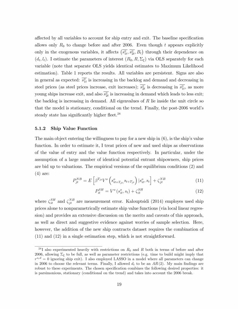
5.1.2 Ship Value Function

The main object entering the willingness to pay for a new ship in (6), is the ship�s value

function. In order to estimate it, I treat prices of new and used ships as observations

of the value of entry and the value function respectively. In particular, under the

assumption of a large number of identical potential entrant shipowners, ship prices

are bid up to valuations. The empirical versions of the equilibrium conditions (2) and

(4) are:

PNBjt = Eh�TjtV o

�soit+Tjt;st+Tjt

�jsoit; st

i+ �NBjt (11)

P SHit = V o (soit; st) + �SHit (12)

where �SHit and �NBjt are measurement error. Kalouptsidi (2014) employes used ship

prices alone to nonparametrically estimate ship value functions (via local linear regres-

sion) and provides an extensive discussion on the merits and caveats of this approach,

as well as direct and suggestive evidence against worries of sample selection. Here,

however, the addition of the new ship contracts dataset requires the combination of

(11) and (12) in a single estimation step, which is not straightforward.

28I also experimented heavily with restrictions on R0 and R both in terms of before and after2006, allowing �� to be full, as well as parameter restrictions (e.g. time to build might imply thatrs1d = 0 ignoring ship exit). I also employed LASSO in a model where all parameters can changein 2006 to choose the relevant terms. Finally, I allowed dt to be an AR (2). My main �ndings arerobust to these experiments. The chosen speci�cation combines the following desired properties: itis parsimonious, stationary (conditional on the trend) and takes into account the 2006 break.

19

rs1o , pre-1.47(0:97)

rs1s11.104(0:04)�

rs2o , pre2.53(1:03)�

rs2s1-0.15(0:04)�

rBo , pre-8.49(7:31)

rBs10.16(0:3)

rs1o , post-1.46(0:98)

rs1s20.08(0:094)

rs2o , post2.53(1:04)�

rs2s20.81(0:1)�

rBo , post-8.5(7:35)

rBs21.07(0:71)�

rd00.41(0:17)�

rs1B0.021(0:0044)�

rd�0.008(0:005)

rs2B-0.007(0:0047)

rd0.69(0:11)�

rBB0.87(0:03)�

rl00.7(0:4)

rs1d0.0046(0:0035)

rl�0.021(0:015)

rs2d0.004(0:0037)�

rl0.8(0:09)�

rBd0.075(0:026)

�s1� 0.0001 rs1l-0.003(0:001)�

�s2� 0.0001 rs2l0.002(0:001)�

�B� 0.004 rBl-0.0094(0:007)

�b� 0.14�d� 1.23

Table 1: VAR parameter estimates. Stars indicate signi�cance at the 0.05 level.

20

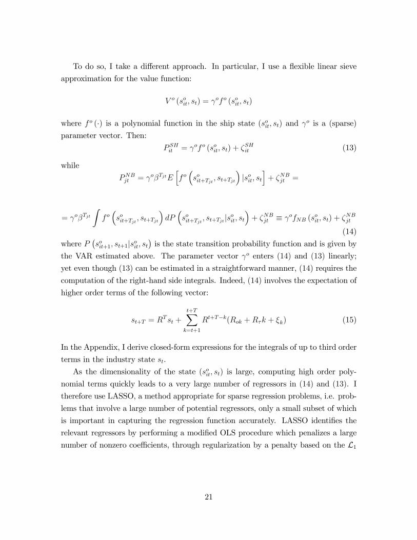
To do so, I take a di¤erent approach. In particular, I use a �exible linear sieve

approximation for the value function:

V o (soit; st) = of o (soit; st)

where f o (�) is a polynomial function in the ship state (soit; st) and o is a (sparse)parameter vector. Then:

P SHit = of o (soit; st) + �SHit (13)

while

PNBjt = o�TjtEhf o�soit+Tjt ; st+Tjt

�jsoit; st

i+ �NBjt =

= o�TjtZf o�soit+Tjt ; st+Tjt

�dP�soit+Tjt ; st+Tjtjs

oit; st

�+ �NBjt � ofNB (soit; st) + �NBjt

(14)

where P�soit+1; st+1jsoit; st

�is the state transition probability function and is given by

the VAR estimated above. The parameter vector o enters (14) and (13) linearly;

yet even though (13) can be estimated in a straightforward manner, (14) requires the

computation of the right-hand side integrals. Indeed, (14) involves the expectation of

higher order terms of the following vector:

st+T = RT st +

t+TXk=t+1

Rt+T�k(Rok +R�k + �k) (15)

In the Appendix, I derive closed-form expressions for the integrals of up to third order

terms in the industry state st.

As the dimensionality of the state (soit; st) is large, computing high order poly-

nomial terms quickly leads to a very large number of regressors in (14) and (13). I

therefore use LASSO, a method appropriate for sparse regression problems, i.e. prob-

lems that involve a large number of potential regressors, only a small subset of which

is important in capturing the regression function accurately. LASSO identi�es the

relevant regressors by performing a modi�ed OLS procedure which penalizes a large

number of nonzero coe¢ cients, through regularization by a penalty based on the L1

21

norm of the parameter of interest. Thus o is estimated from :

min o

(Xj;t

�PNBjt � ofNB (soit; st)

�2+Xi;t

�P SHit � of o (soit; st)

�2+ � j oj1

)

In this application, the regressors f o (soit; st) and fNB (soit; st) are third order polyno-

mials in st and soit, as well as interactions of soit and st. The discount factor is set to

0:9877 which corresponds to 5% annual interest rate.

The �exible nature of this empirical approach implies that the parameters o

embody equilibrium features which are likely to change in 2006 as agents�valuations

are altered (mainly because of the permanently higher �eet and thus competition).

Therefore, in analogy with the VAR formulation, I allow the value function to change

before and after 2006, by adding all monomials multiplied by a post-2006 dummy

variable. Figure 5 depicts the estimated value function on the observed states for zero

year old ships (the relevant value function for the value of entry). Consistent with the

raw data, Chinese ships are of lower value, with Japanese ships being of higher value;

yet the di¤erences are small.29

Figure 5: Value function of a ship at age zero. 0.95 bootstrap con�dence intervals.

5.2 Shipbuilding Production Cost Function

I next turn to estimating the shipbuilding cost function. I begin with the simple case

where shipbuilders are static to illustrate the estimation strategy followed. I present

29Pointwise con�dence intervals are computed via 500 bootstrap samples, with the resamplingdone on the error.

22

the estimation results along with several robustness exercises. I then proceed to the

case of dynamic shipbuilders.

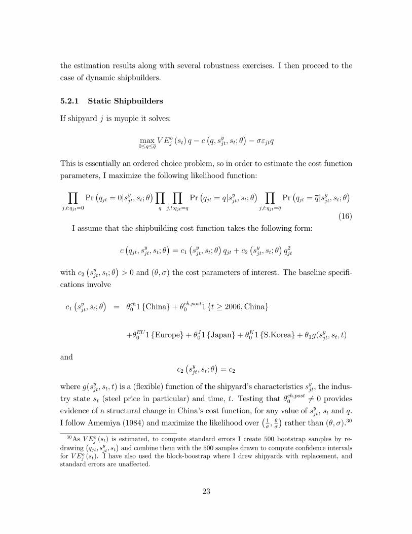
5.2.1 Static Shipbuilders

If shipyard j is myopic it solves:

max0�q�q

V Eoj (st) q � c�q; syjt; st; �

�� �"jtq

This is essentially an ordered choice problem, so in order to estimate the cost function

parameters, I maximize the following likelihood function:Yj;t:qjt=0

Pr�qjt = 0jsyjt; st; �

�Yq

Yj;t:qjt=q

Pr�qjt = qjsyjt; st; �

� Yj;t:qjt=q

Pr�qjt = qjsyjt; st; �

�(16)

I assume that the shipbuilding cost function takes the following form:

c�qjt; s

yjt; st; �

�= c1

�syjt; st; �

�qjt + c2

�syjt; st; �

�q2jt

with c2�syjt; st; �

�> 0 and (�; �) the cost parameters of interest. The baseline speci�-

cations involve

c1�syjt; st; �

�= �ch0 1 fChinag+ �

ch;post0 1 ft � 2006;Chinag

+�EU0 1 fEuropeg+ �J01 fJapang+ �K0 1 fS.Koreag+ �1g(syjt; st; t)

and

c2�syjt; st; �

�= c2

where g(syjt; st; t) is a (�exible) function of the shipyard�s characteristics syjt, the indus-

try state st (steel price in particular) and time, t. Testing that �ch;post0 6= 0 provides

evidence of a structural change in China�s cost function, for any value of syjt, st and q.

I follow Amemiya (1984) and maximize the likelihood over�1�; ��

�rather than (�; �).30

30As V Eoj (st) is estimated, to compute standard errors I create 500 bootstrap samples by re-drawing

�qjt; s

yjt; st

�and combine them with the 500 samples drawn to compute con�dence intervals

for V Eoj (st). I have also used the block-boostrap where I drew shipyards with replacement, andstandard errors are una¤ected.

23

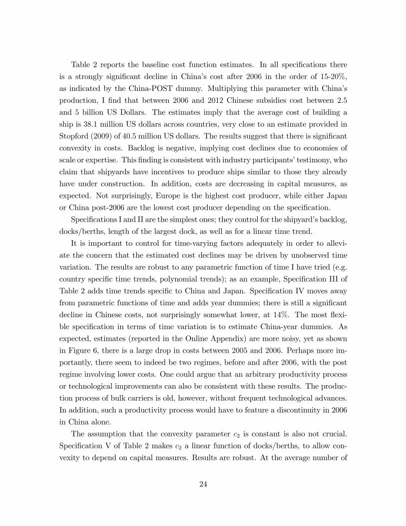
Table 2 reports the baseline cost function estimates. In all speci�cations there

is a strongly signi�cant decline in China�s cost after 2006 in the order of 15-20%,

as indicated by the China-POST dummy. Multiplying this parameter with China�s

production, I �nd that between 2006 and 2012 Chinese subsidies cost between 2:5

and 5 billion US Dollars. The estimates imply that the average cost of building a

ship is 38:1 million US dollars across countries, very close to an estimate provided in

Stopford (2009) of 40:5 million US dollars. The results suggest that there is signi�cant

convexity in costs. Backlog is negative, implying cost declines due to economies of

scale or expertise. This �nding is consistent with industry participants�testimony, who

claim that shipyards have incentives to produce ships similar to those they already

have under construction. In addition, costs are decreasing in capital measures, as

expected. Not surprisingly, Europe is the highest cost producer, while either Japan

or China post-2006 are the lowest cost producer depending on the speci�cation.

Speci�cations I and II are the simplest ones; they control for the shipyard�s backlog,

docks/berths, length of the largest dock, as well as for a linear time trend.

It is important to control for time-varying factors adequately in order to allevi-

ate the concern that the estimated cost declines may be driven by unobserved time

variation. The results are robust to any parametric function of time I have tried (e.g.

country speci�c time trends, polynomial trends); as an example, Speci�cation III of

Table 2 adds time trends speci�c to China and Japan. Speci�cation IV moves away

from parametric functions of time and adds year dummies; there is still a signi�cant

decline in Chinese costs, not surprisingly somewhat lower, at 14%. The most �exi-

ble speci�cation in terms of time variation is to estimate China-year dummies. As

expected, estimates (reported in the Online Appendix) are more noisy, yet as shown

in Figure 6, there is a large drop in costs between 2005 and 2006. Perhaps more im-

portantly, there seem to indeed be two regimes, before and after 2006, with the post

regime involving lower costs. One could argue that an arbitrary productivity process

or technological improvements can also be consistent with these results. The produc-

tion process of bulk carriers is old, however, without frequent technological advances.

In addition, such a productivity process would have to feature a discontinuity in 2006

in China alone.

The assumption that the convexity parameter c2 is constant is also not crucial.

Speci�cation V of Table 2 makes c2 a linear function of docks/berths, to allow con-

vexity to depend on capital measures. Results are robust. At the average number of

24

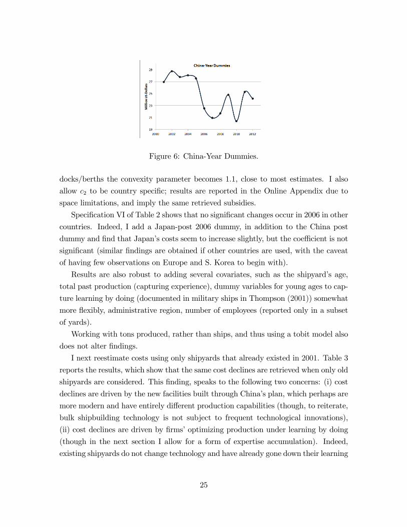
Figure 6: China-Year Dummies.

docks/berths the convexity parameter becomes 1:1, close to most estimates. I also

allow c2 to be country speci�c; results are reported in the Online Appendix due to

space limitations, and imply the same retrieved subsidies.

Speci�cation VI of Table 2 shows that no signi�cant changes occur in 2006 in other

countries. Indeed, I add a Japan-post 2006 dummy, in addition to the China post

dummy and �nd that Japan�s costs seem to increase slightly, but the coe¢ cient is not

signi�cant (similar �ndings are obtained if other countries are used, with the caveat

of having few observations on Europe and S. Korea to begin with).

Results are also robust to adding several covariates, such as the shipyard�s age,

total past production (capturing experience), dummy variables for young ages to cap-

ture learning by doing (documented in military ships in Thompson (2001)) somewhat

more �exibly, administrative region, number of employees (reported only in a subset

of yards).

Working with tons produced, rather than ships, and thus using a tobit model also

does not alter �ndings.

I next reestimate costs using only shipyards that already existed in 2001. Table 3

reports the results, which show that the same cost declines are retrieved when only old

shipyards are considered. This �nding, speaks to the following two concerns: (i) cost

declines are driven by the new facilities built through China�s plan, which perhaps are

more modern and have entirely di¤erent production capabilities (though, to reiterate,

bulk shipbuilding technology is not subject to frequent technological innovations),

(ii) cost declines are driven by �rms�optimizing production under learning by doing

(though in the next section I allow for a form of expertise accumulation). Indeed,

existing shipyards do not change technology and have already gone down their learning

25

curve.

As regional governments in China can play an important role (see Section 2), I

consider a speci�cation where they implement the national plan at di¤erent dates

and magnitudes. As no o¢ cial documentation was found on implementation dates, I

consider the �rst quarter that new shipbuilding docks/berths come online and divide

regions into three groups. I present results in the Online Appendix, which are similar

to prior speci�cations. It seems that the last region to implement, also has the lowest

subsidy level.

One may be concerned that the estimated cost declines are somehow driven by

the estimated willingness to pay, V Eoj (st), (for instance due to the di¤erent pre and

post expectations -V AR model- and LASSO coe¢ cients). To address this concern

I estimate costs using the average quarterly price (across shipyards and countries)

of a new ship, which is reported by Clarksons. I �nd that estimated subsidies are

signi�cant and of the same magnitude.

One might also worry that there was a coincident increase in demand for ships by

Chinese shipowners; as discussed in Section 2, however, the overwhelming majority

of Chinese built ships are in fact exported.

Finally, note that when shipyards choose production in a static fashion, the as-

sumption that dock development is determined by higher administration rather than

the yards themselves, does not bias cost (and thus subsidy) estimates in this model

(the �rst order condition for optimal production is una¤ected by shipyard dock choice).31

When shipyards take into account production dynamics, however, this assumption is

important; if yards were to choose both production and docks, the �rst order con-

ditions are no longer decoupled, since �rms consider the future impact of all their

actions.

31If shipyards were choosing docks themeselves and the government provided subsidies to bothoperating costs, as well as dock building costs, it is easy to show that both cost and dock buildingsubsidies can be separately identi�ed. In addition this does not hinge upon the speci�c cost functionemployed here, but rather it holds under fairly general cost function speci�cations.

26

I II III IV V VI

China32.4(5:75)��

33.34(5:95)��

33.56(5:8)��

31.23(5:13)��

36.83(6:81)��

32.23(5:84)��

China, POST-7.67(2:42)��

-7.63(2:54)��

-8.01(3:82)��

-4.21(1:85)��

-8.85(3:06)��

-6.51(2:63)��

Europe33.14(6:04)��

34.14(6:31)��

36.23(7:61)��

31.76(5:31)��

37.21(7:08)��

33.38(5:99)��

Japan25.4(3:78)��

25.94(3:78)��

26.02(4:16)��

28.14(3:62)��

30.02(4:68)��

25.14(3:58)��

Japan, POST1.085(1:47)

S. Korea31.34(5:52)��

32.41(5:44)��

34.85(7:3)��

32.46(4:54)��

34.29(5:85)��

32.22(5:43)��

Backlog-0.71(0:18)��

-0.71(0:18)��

-0.72(0:18)��

-0.39(0:17)��

-0.8(0:202)��

-0.66(0:17)��

Docks/Berths-0.17(0:17)��

-0.17(0:18)

-0.16(0:16)

Max Length-0.0011(0:0011)

-0.0011(0:0012)

-0.001(0:0011)

Steel price0.38(0:24)

0.38(0:23)

0.38(0:24)�

0.87(0:5)��

0.44(0:24)�

0.36(0:22)

t0.33(0:06)��

0.33(0:06)��

0.28(0:084)��

0.36(0:07)��

0.3(0:06)��

China*t0.068(0:13)

Japan*t0.062(0:09)

c21.31(0:34)��

1.31(0:35)��

1.33(0:36)��

0.71(0:32)��

1.22(0:33)

c2 � (Docks/Berths)0.32(0:097)��

�14.15(3:48)

14.11(3:85)

14.36(3:59)

7.49(3:3)

17.08(4:15)

13.1(3:27)

Year Dummies NO NO NO YES NO NO

Table 2: Baseline static cost function estimates. Time t measured in quarters. Coun-tries refer to country dummy variables. Stars indicate signi�cance at the 0.05 level.Standard errors computed from 500 bootstrap samples.

27

China41.02(10:61)��

China,POST-9.15(4:1)��

Europe41.65(11:19)��

Japan30.5(6:51)��

S. Korea38.1(9:52)��

Backlog-1.002(0:34)��

Docks/Berths-0.375(0:26)

Max Length0.0006(0:0023)

Steel price0.36(0:36)

t0.38(0:097)��

c21.84(0:63)��

�18.69(6:16)

Table 3: Static cost function estimates with yards existing prior to 2001. Time tmeasured in quarters. Countries refer to country dummy variables. Stars indicatesigni�cance at the 0.05 level. Standard errors computed from 500 bootstrap samples.

28

5.2.2 Dynamic Shipbuilders

I now examine the case where shipyards take into account the dynamic feedback of

their current production choice to their future operating costs, as well as the durability

of their product. The shipyard�s optimal production now obeys (9). To ease notation,

rename the shipyard state x =�syjt; st

�and x0 =

�syjt+1; st+1

�and suppress (j; t).

Recall the optimal policy thresholds that de�ne the shipyard�s optimal production

(see Lemma 1):

A (x; q) =1

�[V Eo (x) + (c (q; x)� c (q + 1; x)) + � (CV y (x; q + 1)� CV y (x; q))]

(17)

for q = 0; 1; :::; q � 1. To estimate the parameters (�; �), I maximize the likelihood(16) with choice probabilities:

Pr (q� = 0jx) � p0 (x) = Pr (" � A (x; 0)) (18)

Pr (q� = qjx) � pq (x) = Pr (" � A (x; q � 1))� Pr (" � A (x; q))

Pr (q� = qjx) � pq (x) = Pr (" � A (x; q � 1))

Maximizing this likelihood function would be trivial if the continuation value

CV y (x; q) were known. This is the standard di¢ culty of estimating dynamic se-

tups and to address it, I adopt a novel approach that proceeds in two steps (following

the recent literature, e.g. Hotz and Miller (1993) and Bajari, Benkard and Levin

(2007)). First, I invert observed choice probabilities to directly obtain the optimal

policy thresholds nonparametrically. Second, I show that the latter lead to a closed-

form expression for ex ante optimal per period payo¤s, which in turn are su¢ cient to

obtain the value function. I next describe my approach in detail.

For the �rst step, note from (18) that clearly, the choice probabilities are a one-

to-one function of the optimal policy thresholds A (x; q). Therefore the latter can be

29

recovered from the observed choice probabilities using32:

A (x; q) = ��1

1�

qXk=0

pk (x)

!; for q = 0; 1; :::; q � 1 (19)

where � (�) is the standard normal distribution. Note that A (x; q) is (weakly) de-creasing in q. Most important, if A (x; q) is known, so is the optimal policy: for any

(x; "),

q� (x; ") = bq; such that " 2 [A (x; bq) ; A (x; bq � 1)]For the second step, I show that once the optimal policy is known, the value

function can be recovered in a straightforward manner. Indeed, consider shipyard j�s

Bellman equation (7) which I repeat here for convenience:

V y (x; ") = max0�q�q

�y (x; q; ") + �E"0;x0 [Vy (x0; "0) jx; q]

where �y (x; q; ") � V Eo (x) q � c (q; x)� �q". The ex ante value function under therecovered optimal policy becomes:

V y (x) � E"V y (x; ") = E" [�y (x; q� (x; ") ; ") + �E"0;x0 [V y (x0; "0) jx; q� (x; ")]] (20)

If the ex ante per period pro�t, E"�y (x; q� (x; ") ; "), were known, then one could

solve for the ex ante value function from (20). This can be done in several ways,

such as state space discretization and matrix inversion, or parametric approximation;

I opt for the latter because of the large dimension of the state space. In particular, I

approximate the value function by a polynomial function of the state, so that:

V y (x) = yf y (x)

then (20) becomes

(f y (x)� �E" [f y (x0) jx; q� (x; ")]) y = E"�y (x; q� (x; ") ; ") (21)

It is now possible to estimate the approximating parameters y by ordinary regression,

32To show this, begin with p0 (x) = 1 � � (A (x; 0)), so that A (x; 0) = ��1 (1� p0 (x)).Next, p1 (x) = � (A (x; 0)) � � (A (x; 1)) = 1 � po (x) � � (A (x; 1)), so that A (x; 1) =��1 (1� p0 (x)� p1 (x)). The general case follows by induction.

30

provided the ex ante pro�t can be computed. Note, however, that the large number of

states leads to an exploding number of possible terms in f y (x); in addition, choosing

which terms to include in f y (x) can be an arduous process. Instead, I estimate the

sparse vector y via LASSO, which circumvents these issues. Using LASSO to solve

for approximate value functions can be useful to the many empirical applications of

dynamic setups.

I now only need to show how E"�y (x; q� (x; ") ; ") is computed. Under the assump-

tion of quadratic costs, ex ante per period payo¤s become:

E"�y (x; q� (x; ") ; ") =

= E"�V Eo (x) q� (x; ")� c1 (x; �) q� (x; ") + c2 (x; �) q� (x; ")2 � �q� (x; ") "

�= (V Eo (x)� c1 (x; �))E"q� (x; ") + c2 (x; �)E"q� (x; ")2 � �E" [q� (x; ") "]

(22)

I show in the Appendix that

E"q� (x; ") =

q�1Xq=0

� (A (x; q)) (23)

E" [q� (x; ")]2 = 2

qXq=1

q� (A (x; q � 1))�q�1Xq=0

� (A (x; q)) (24)

E" [q� (x; ") "] = �

q�1Xq=0

� (A (x; q)) (25)

where � (�) is the standard normal density.To sum up, the estimation proceeds as follows (further details are in the Appendix):

1. Estimate the policy thresholds A (x; q) using (19)

2. Compute the statistics of the optimal production in (23), (24) and (25)

3. At each guess of the parameters (�; �) in the optimization of the likelihood (16):

31

(a) Solve for the approximate value function parameters y from (21)

(b) Using y, compute the choice probabilities and update (�; �).

Table 4 gives the maximum likelihood estimate of the cost function of dynamic

shipyards. The implied subsidy is in the order of 20% or 5:6 billion US dollars paid

between 2006 and 2012, similarly to the case of static shipyards. Also in analogy

to static shipbuilders, costs are decreasing in the current backlog, consistent with

economies of scale or accumulation of expertise. More docks/berths, as well as longer

docks decrease costs. Interestingly, the estimated cost function of dynamic shipyards

is signi�cantly more convex than the one of static shipyards. Since accumulating a

backlog decreases future costs and yards take this into account, higher cost parameters

are needed to justify the observed low production levels.

Finally, I compute the expected value of all new Chinese shipyards that are born

through China�s government plan, which equals 8:5 billion US dollars. One can think

of this amount as a rough estimate of the order of magnitude of the costs of building

these shipyards.

In summary, the static and dynamic formulations yield similar results in terms of

subsidy detection, with the dynamic model having a higher likelihood. As discussed in

the following section, however, the two models have di¤erent quantitative predictions

regarding the implications of subsidies.

32

China46.12(9:08)��

China,POST-8.9(3:32)��

Europe47.42(9:62)��

Japan35.88(5:76)��

S. Korea45.63(8:31)��

Backlog-0.84(0:23)��

Docks/Berths-0.22(0:15)

Max Length-0.002(0:0014)

Steel price0.36(0:24)

t0.25(0:067)��

c22.53(0:69)��

�19.75(5:26)��

Table 4: Dynamic cost function estimates. Time t measured in quarters. Coun-tries refer to country dummy variables. Stars indicate signi�cance at the 0.05 level.Standard errors computed from 500 bootstrap samples.

6 Quantifying the Implications of Subsidies

I quantitatively assess the degree to which industrial subsidies contribute to China�s

rapid emergence as a world leader in the shipbuilding industry. In particular, I evalu-

ate the impact of government interventions on industry prices, production reallocation

across countries, costs and consumer surplus. I use my model to predict the evolution

of the industry in the absence of China�s government shipbuilding plan, by removing

both the cost subsidies retrieved in Section 5, as well as the new shipbuilding facilities

that were built through the plan. This counterfactual quanti�es the adverse trade

e¤ects from these two interventions, which are considered actionable by the WTO.

Moreover, I assess the relative contribution of the new shipyards to industrial reallo-

33

cation and surplus by performing a counterfactual that removes the new facilities but

maintains the detected cost subsidies.

To implement the main counterfactual of �no interventions�, I assume that shipown-

ers maintain their pre-2006 expectations and ship value functions, shipyards keep their

pre-2006 costs and capital structure (i.e. docks/berths and length) and new ship-

yards are removed. To implement the �no entrants� counterfactual, new shipyards

are removed and existing shipyards keep their post-2006 cost functions and capital

structures. Also, I assume that shipowners switch to the post-2006 expectations and

value functions. In other words, shipowners understand that a change occurred; yet

they can�t distinguish between di¤erent policies. I feed the observed post-2006 values

for shipping demand and steel prices into the model and simulate shipyard optimal

production and ship prices. Computing the equilibrium to the model is not straight-

forward and thus details on the implementation of these counterfactuals can be found

in the Appendix.

As shown in Table 5, the industrial subsidies lead to substantial reallocation in

production, by increasing China�s market share and decreasing Japan�s share: if the

plan is removed, China�s market share falls from 50% to less than 20%. Japan�s

share increases from 43% to 74% in the absence of China�s intervention.33 If only the

new shipyards are removed, China�s share falls from 50% to 40%, revealing that new

facilities played an important but not the predominant part in China�s expansion.

Table 5 also compares ship prices in the baseline and counterfactual worlds and

shows that ship prices are higher for all countries in the absence of China�s subsidiza-

tion plans (by about 5%). This is not surprising, given that China�s subsidization

shifted supply outward.

Next, I turn to costs, pro�ts and shipper surplus, shown in the lower half of Table

5. China�s government plan decreased pro�ts of other countries by moderate amounts;

for example, Japan�s pro�ts fell by 11% because of Chinese subsidies between 2006

and 2012. In this model, shipowners neither gain, nor lose from subsidies: because

of the free entry condition in shipping, they are always indi¤erent between buying a

ship or not (existing shipowners do lose, however, because of the unexpected negative

shock to their asset value). Shippers of cargo, however, gain from subsidies as they

lead to higher shipbuilding production and thus to a larger �eet. I use the demand

33Counterfactual results are robust to the assumption that c2 is constant; I replicated the coun-terfactuals in the case of static shipyards under cost speci�cation V of Table 2, where c2 is linear inthe number of docks/berths.

34

Baseline No Interventions No New FacilitiesMarket Share, China 50% 18.4% 40%Market Share, Japan 43.4% 73.9% 54.7%Ship Price, China 23.8 25 24.2Ship Price, Japan 25.5 26.6 25.95

Japan, Shipyard Pro�ts 95.1 105.4 102.8Freight Rate (price per voyage) 1.25 1.28 1.27Consumer Surplus (shippers) 5617 5331 5446Industry AVC 0.42 0.65 0.54

Table 5: Counterfactual results. Prices, surplus and average variable cost (AVC)measured in million US Dollars. Pro�ts and surplus refer to the total amount between2006 and 2012.

curve estimated in the Appendix to compute shipping prices and shipper surplus.34

As shown in Table 5, the freight rate is moderately higher (by 3%) in the absence

of Chinese subsidies. The di¤erence in prices, however, increases over time between

2006 and 2012: because of time to build it takes time until the di¤erent worlds lead

to di¤erent �eet levels. Indeed, between 2009 and 2012 prices are higher by 5%. As a

result, cargo shippers bene�t from Chinese subsidies; their consumer surplus is higher

by 5% because of subsidies and increases over time (between 2009 and 2012 consumer

surplus is higher by 8%). Note that between 2006 and 2012 the cost subsidies alone

(i.e. ignoring the additional costs of building new yards), cost the government about

5:6 billion US dollars and resulted in consumer surplus gains of 286 million US dollars.

This calculation implies that a frequent assertion that China developed shipbuilding

to bene�t from low freight rates for its trade seems to be unsubstantiated; indeed,

the bene�ts of subsidies within the maritime industries are minimal and perhaps the

Chinese government is aspiring to externalities to di¤erent sectors (e.g. steel, defense)

or, even, national pride (Grossman (1990)).

Next, I turn to the cost implications of subsidies. I compute the average cost

of a ship at the industry level and �nd that as expected, subsidies decrease costs of

production, see last row of Table 5. If I decompose the average cost to subsidies and

market share allocation, however, this picture is entirely di¤erent. Indeed, consider

34The cargo shipping demand curve gives the price per voyage as a function of the total numberof voyages. I assume that there is a constant �eet utilization rate to map the �eet into voyages.

35

the cost function cjq+ cq2, for j 2 fChina, EU, Japan, S.Koreag, which for j =Chinabecomes (cchina � s) q + cq2 post-2006. The change in the industry average cost be-cause of subsidies is equal to a sum of two terms: the �rst is s qChina

qChina+qEU+qJapan+qSK,

while the second includes all other terms and is related to the reallocation of pro-

duction and market share. As implied by the numbers in Table 5, the change in

industry average cost brought about by production subsidies is 0:23 million. The

term s qChinaqChina+qEU+qJapan+qSK

equals 4:44 million, implying a negative reallocation ef-

fect equal to 0:23 � 4:44 = �4:21 million. In other words, the subsidization in costsshould have led to a much larger decline in the industry average cost of production;

but as subsidies shift production away from the low-cost Japanese shipyards towards

the high-cost Chinese shipyards, the industry produces at a much higher average cost

net of subsidies.

Finally, there are two questions of interest related to the importance of allowing

for dynamics in shipbuilding production. First, how important is the interaction of

subsidies and dynamics in production? In the case of production dynamics, increased

backlog decreases costs and thus market share gains multiply and may lead to more

reallocation favorable to China and unfavorable to Japan. Indeed, when I simulate

the model setting the impact of backlog in the cost function equal to zero, I �nd that

reallocation would have been somewhat lower in the absence of dynamics: about 7%

of China�s increase in market share can be attributed to the dynamic production feed-

back. The second question of interest, is whether the static model leads to di¤erent

counterfactual results. To answer, I use speci�cation II of Table 2 to simulate the

model. I �nd that even though the static and dynamic models yield similar results

in terms of detecting subsidies, they lead to di¤erent predictions regarding the impli-

cations of subsidies. In particular, I �nd that the static model leads to signi�cantly

more reallocation than the dynamic model: China�s loses 73% of its market share in

the absence of subsidies, while Japan�s share almost doubles. This di¤erence is mainly

driven by the di¤erent cost function, which is higher and more convex in the case of

dynamic shipyards.

7 Conclusion

The role of industrial policy in China�s rapid takeover, especially in industries that are

capital intensive, is still an open question. To answer, one needs to �rst know what

36

policies are in place. This paper measures subsidies and quanti�es their impact for the

striking example of the world shipbuilding industry. I �nd strong evidence consistent

with subsidies that decreased shipyard costs by 15-20%. The interventions led to

a substantial reallocation of production across countries with no signi�cant surplus

gains. Therefore, subsidies may be justi�ed by shipbuilding�s important externalities

to other sectors, such as the steel industry or the readiness of the military sector. Yet,

understanding government objectives is an interesting avenue for future research.

8 Appendix

8.1 Creation of shipping demand state

I estimate the inverse demand for shipping services via instrumental variables regres-

sion, to create the state dt. The analysis follows Kalouptsidi (2014). The empirical

analogue of the demand curve in (1) chosen is:

Pt = �d0 + �

d1X

dt + �

d2Q

ot + "

dt (26)

where Pt is the average price per voyage observed in a quarter, Xdt includes demand

shifters, while Qot is the total number of voyages realized (see Kalouptsidi (2014)

for a detailed data description). Xdt includes the index of food prices, agricultural

raw material prices and minerals prices (taken from UNCTAD), the world aluminum

(taken from the International Aluminum Institute) and world grain production (taken

from the International Grain Council), as well as the Handymax �eet (as a potential

substitute). The �rst stage instruments include the total �eet and its mean age. Both

instruments are key determinants of industry supply capacity, as ship operating costs

are convex and depend on age. Instrumentation corrects both for endogeneity, as

well as measurement error (I observe the number of voyages realized, rather than

ton-miles).

Table 6 reports the results. The impact of all shifters is lumped into the state

variable dt (the residual b"dt is included in dt as it captures omitted demand shifters):dt =

c�d1Xdt +

b"dt

37

1st stage 2nd stageparameter parameter/106

constant-2731.3(790:28)��

-1.403(1:26)

food P0.61(0:693)

0.0051(0:0038)

agr raw mat P1.35(0:48)��

0.0022(0:0028)

mineral P-0.43(0:33)

0.0014(0:0018)

aluminum prod-0.28(0:11)��

0.0012(0:00057)��

grain prod-0.86(0:9)

0.0047(0:0044)

subst �eet0.38(0:15)��

-0.0022(0:00052)��

�eet0.55(0:22)��

mean age �96.67(18:5)��cQot -0.0033

(0:001)��

Table 6: Demand IV regression results.

8.2 Derivation of state expectations in ship value function

I derive the expressions required for the LASSO estimation of the value functions of

Section 5:1:2. Remember that I approximate the value function with a polynomial

function, so that:

V o(xt) = of o (xt) =

dXi=1

oix(i)t

where xt = (soit; st), and x(i)t are Kronecker products, so that x(2)t = xt xt, x(3)t =

x(2)t xt, etc. Then, (14) can be written as:

PNBjt = �Tjt oE�f o�xt+Tjt

�jxt�= �Tjt

dXi=1

oiE�x(i)t+Tjt

jxt�

(27)

The conditional expectation is only necessary for st since soit evolves deterministi-

38

cally. I use the general VAR model (6) to get that:

st+T = � (t+ T; t) st +

t+TXk=t+1

� (t+ T; k) (R0k + �k)

where

� (t+ T; k) =

(Rt+TRt+T�1:::Rk+1; for k < t+ T

I; for k = t+ T

I denotes the identify matrix. In the time invariant case, Rt = R, all t, I get (15) of

the main text.

Next, I focus on the time invariant case. The above expression takes the form:

st+T = A+ v

where

A = RT st +t+TXk=t+1

Rt+T�kR0k

v =t+TXk=t+1

Rt+T�k�k

Note that conditional on st, A is constant. Moreover, v is zero-mean normal with

covariance:

�v = Ev0v =

t+TXk=t+1

Rt+T�k�� (R0)t+T�k

Therefore, (27) becomes:

PNBjt = �TjtdXi=1

oiE�(A+ v)(i) jxt

�I next compute the conditional expectations for up to third order terms:

E (A+ vjxt) = A

E�(A+ v)(2) jxt

�= A(2) + vec (�v)

E�(A+ v)(3) jxt

�= A(3) + A vec (�v) + vec (�v) A+ Tmm2A vec (�v)

39

where vec (x) denotes the vector formed by stacking the columns of x one after the

other; the matrix Tmm2 is de�ned as the following linear operator: given a L�nmatrixA, TLn is an Ln � Ln matrix speci�ed by the assignment TLnvec (A) = vec (A0), (A0

stands for transpose). The �rst of the above equations is straightforward. To prove

the second, use:

E�(A+ v)(2) jxt

�= E

�(A+ v)(2)

�= A A+ A E (v) + E (v) A+ Ev(2)

It is easy to see that Ev(2) = vec (Evv0) = vec (�v) using the property

vec (BXC) = (C 0 B) vec (X)

Finally, I prove the third order equation. Note that

E�(A+ v)(3) jxt

�= A E (A+ v)2 + Ev (A+ v)2

= A�A(2) + vec (�v)

�+ E (v A v) + E (v v A) + Ev(3)

Ev(3) is zero since v is Gaussian. Moreover,

E (v A v) = Tmm2 Ev(2)

Indeed, if B and C are matrices of dimensions (L; n) and (n; k) respectively, then

B C = Tpl (C B)Tnk

8.3 Statistics of the Optimal Production

To derive (23), I use (18) to get:

E"q� (x; ") =

qXq=1

qpq (x) =

q�1Xq=1

q [� (A (x; q � 1))� � (A (x; q))] + q� (A (x; q � 1))

=

q�2Xq=0

(q + 1)� (A (x; q))�q�1Xq=1

q� (A (x; q)) + q� (A (x; q � 1))

= � (A (x; 0)) +

q�2Xq=1

� (A (x; q)) + � (A (x; q � 1)) =q�1Xq=0

� (A (x; q))

40

Equation (24) follows similarly. Finally, let � (") denote the standard normal

density. Then, Z b

a

"� (") = � 1

2p�

Z b

a

de�12"2 = � (a)� � (b)

and therefore:

E""q� (x; ") =

Z"q� (x; ")� (") d" =

=

q�1Xq=1

q

Z A(x;q�1)

A(x;q)

"� (") + q

Z A(x;q�1)

�1"� (")

=

q�1Xq=1

q [�(A (x; q))� � (A (x; q � 1))]� q� (A (x; q � 1))

= �q�1Xq=0

�(A (x; q))

8.4 Estimating costs for dynamic shipbuilders: Details

I provide details on each step performed when estimating the cost function of dynamic

shipyards.

Step 1: Estimate A (x; q) using (19). In this step, I �rst compute the choice

probabilities fpq (x)gqq=0 from observed frequencies. I also include a post-2006 dummyin the state to capture di¤erences in the policy function before and after 2006. As is

common in dynamic applications, there are not many observations for all q = 0; 1; :::; q

at each state x. Therefore, I �rst cluster the data �nely, using the kmeans algorithm,

and then compute frequencies on this subset of states. Second, I smooth the frequency

matrix using kernels. In particular, I compute the choice probability pq (x) at state x

using the following formula:

pq (x) =Xx0

w (x0 � x) epq (x0)where epq (x) is the observed frequency count of q at state x and w (�) is a kernelthat appropriately weights the distance of x from every other state x0. For numerical

states (backlog, docks/berths, length, time, �eet, total backlog, demand, steel price)

I use normal kernels with diagonal covariance. For categorical states (country and

41

post-2006 dummy) I use the kernel:

w (x0 � x) =(1� h; if x0 = xh=kx; if x0 6= x

where kx is the number of values that x can take (in the case of country it�s 4, in

the case of the post dummy 2) and h represents the bandwidth of the kernel. As

h gets close to 0, this kernel weights states that share the same variable x. I also

experimented with parametric speci�cations for A (x; q). In particular, I estimated an

ordered probit model using directly the production data, so that:

A (x; q) = �f (x) + q

while the observed variables are the production values given by

q� (x; ") = bq; such that " 2 [A (x; bq) ; A (x; bq � 1)]I estimate � and q for q = 0; :::; q � 1 via Maximum Likelihood. This speci�cation

is �exible in terms of q but less so in terms of x.35 It overall gives similar results

to the nonparametric speci�cation above. Finally, I chose q = 10, since 99:75% of

observations involve q � 10.Step 2: Compute the terms Eq�, Eq�2, E"q using (23), (24) and (25).

Step 3: At each guess of the parameters (�; �) in the optimization of the likelihood

(16) the following calculations are performed:

Step 3a: Solve for the approximate value function parameters y from (21). Note

that the choice probabilities require the continuation valueCV y (x; q) = yE [f y (x0) jx; q].To estimate y from (21) I need

E";x0 [fy (x0) jx; q� (x; ")] = y

qXq=0

pq (x)Ex0 [fy (x0) jx; q] (28)

35The plot of q with respect to q is close to a linear graph. This is consistent with the staticmodel where

A = ��1�1

�(V E � c1 � c2 (2q + 1))

�This is relevant in case one thought that (in the static case) imposing both a distributional assumptionon "�s, as well as a parametric form on c (q) is restrictive.

42

I use polynomials of third order in all variables (I have also tried fourth order which

doesn�t alter the results). The industry state s evolves by the estimated VAR model

described in Section 5.1.1, while the expectations of its polynomial powers are given

in Appendix 8.3. I assume that the shipyard�s individual backlog, bjt, transitions as

follows:

bjt+1 = (1� �) bjt + q

i.e. �% of the backlog is delivered and q orders of period t enter the backlog. I exper-

imented extensively with the above transition rule. In particular, I have conducted

experiments with time-varying �; for example, � drawn from a probability distribution

estimated from the data (e.g. beta distribution whose mean can depend on the ship-

yard�s current backlog, docks/berths or length; � taken as a discrete random variable

with probabilities estimated from the data); alternatively other experiments employed

deliveries, instead of �, described by a binomial random variable whose parameters

can again depend on shipyard observables. It was found that the simple model where

� is constant over shipyards and time and equal to the sample mean (which is 10%)

performs equally well compared to more complex models. Given the state transitions

it is straightforward to compute (28). I estimate (21) using LASSO in two ways.

First, call the LASSO within the likelihood maximization with the regularization pa-

rameter chosen using Belloni and Chernozhukov (2011). Second, estimate (21) with

LASSO using pro�ts obtained from the static cost estimates. The goal here is to

recover which polynomial terms should be kept. I then run OLS within the likelihood

with only these terms (and repeat the estimation for many values of the regularization

parameter). Results are overall robust to all of the above.

Step 3b: Using y, compute choice probabilities in the likelihood and update (�; �).

A concern in two-step approaches to dynamic frameworks is that the �rst stage

policy functions (in this case, the nonparametric A (x; q) that I recover) may be di¤er-

ent from the optimal policy computed using the true parameters and value function,

i.e. from (17). To check this, I compute A (�) from (17) and �nd that it is close to

its �rst stage estimate. I then re-optimize the likelihood using the new A (�). Theparameters that I report result from this loop.

43

8.5 Counterfactual Computation

There are two steps in the implementation of the counterfactual scenarios presented in

Section 6. First, I compute the equilibrium of the model in each scenario (if shipyards

are static this step is skipped). Second, I simulate the model using the observed paths

of demand and steel prices which are exogenous. Note that if one is only interested in

the �no interventions�counterfactual, one can simply use the pre-2006 expectations

and value functions and simulate the model.

To predict how the industry would evolve under di¤erent counterfactual scenarios

I need to obtain shipyards�optimal policies and value functions under each scenario.

I can no longer use the estimated VAR for state transitions, since this formed an

approximation to expectations that hid equilibrium features. I therefore turn to the

following state transitions for�so1t; s

o2t; Bt

�, where so1t is the number of ships younger

than 20 years old, so2t is the number of ships older than 20 years old and Bt is the

total backlog:

so1t+1 = �Bt + (1� �1t) so1t (29)

so2t+1 = so2t + �1tso1t � � (st)

Bt+1 = (1� �)Bt +Xj

qjt (30)

where � (st) is the number of ships that exit at state st, �1t is the percentage of ships

that transit from 19 years old and 3 quarters to 20 years old and � is the percentage of

the backlog that is delivered, consistent with the individual backlog transition used in

the estimation and described in Appendix 8.5. In words, the number of young ships

so1t+1 equals last period�s young ships plus deliveries from the total backlog, minus

exiting ships (as documented in Kalouptsidi (2014) there is virtually no exit in ships

younger than 20 years old). The number of old ships so2t+1 equals last period�s old

ships plus the aging ships minus exiting ships. Finally, total backlog Bt+1 equals last

period�s total backlog minus deliveries, plus total new ship orders. I calibrate �1t to

3% which is the sample average. To predict ship exit � (st) I follow Kalouptsidi (2014)

where the number of exiting ships is regressed on the industry state (in particular,

log �t = ��st); note that exit rates are extremely low (even during the 2008 crisis).

Demand dt and steel price lt retain their original transition processes, since these are

exogenous to this model.

44

To �nd the equilibrium of the model I use a �xed point algorithm with the goal

of recovering the shipyard�s optimal policy function p�q (x), for all production levels

q and states x = (sy; s), as well as the shipyard�s value function W � (x). At each

iteration l I use the policies plq (x) to update to pl+1q (x) and I keep iterating until

jjpl+1q (x)� plq (x) jj � eps. Each iteration performs the following steps:Step 1: Update the value function using a sparse parametric approximation and

LASSO (third order polynomials are used). The estimation of the value function

approximating parameters, e y, relies on the approximate Bellman equation:�f y (x)� �E

�f y (x0) jplq (x) ; x

�� e y;l+1 = E" ��y(x; q; "); plq (x)�where ex ante pro�ts are computed by:

E"��y(x; q; "); plq (x)

�= [V E (x)� c1 (x)]

qXq=0

qplq (x)�c2qXq=0

q2plq (x)+�

q�1Xq=0

�(Al (x; q))

where A (x; q) = ��1�1�

Pqk=0 p

lk (x)

�, q = 0; 1; :::; q � 1. To derive the above, use

(22) and (25).

Moreover, to compute E�f (x0) jplq (x) ; x

�, I simulate dt and lt one period forward

since these are the only stochastic states now. State transitions are computed via

(29). Due to computational constraints I have assumed throughout that shipyards

keep track of the total backlog rather than the distribution of backlogs. Therefore, at

this stage shipyards don�t have the full information to predict total orders accurately.

To circumvent this issue I make the simplifying assumption that shipyards believe

they are all at the same state and can predict total orders using the total number of

�rms.

Step 2: Update the choice probabilities:

pl+10 (x) = 1� ��1

�

�V Eo (x)� c1 (x)� c2 + �

�CV y;l+1 (1)� CV y;l+1 (0)

���pl+1q (x) = �

�1

�

�V Eo (x)� c1 (x)� c2 (2q � 1) + �

�CV y;l+1 (q)� CV y;l+1 (q � 1)

����

���1

�

�V Eo (x)� c1 (x)� c2 (2q + 1) + �

�CV y;l+1 (q + 1)� CV y;l+1 (q)

���pl+1q (x) = 1�

q�1Xq=0

pl+1q (x)

45

I solve the above �xed point under three scenarios: the true post-2006 world, a

world with no China intervention and a world without the Chinese new shipyards.

These worlds di¤er in the shipyard cost function, the set of active shipyards and the

shipyard capital structure. I perform the �xed point on all data (as a robustness I

have also used a set of states chosen by the kmeans algorithm, as well as the pre-2006

data alone for the relevant counterfactuals).

Finally, to simulate the model, I draw cost shocks " and obtain the corresponding

optimal production using (9) which in turn relies on the value function computed

using the parameters e y retrieved by the �xed point algorithm. At each state visitedI compute E

�f (x0) jp�q (x) ; x

�using the retrieved equilibrium choice probabilities.

References

[1] Aguirregabiria, Victor, and Pedro Mira. 2007. �Sequential Estimation of Dynamic

Discrete Games�. Econometrica 75 (1): 1-53.

[2] Amemiya, Takeshi. 1984. �Tobit Models: A Survey�. Journal of Econometrics.

24: 3-61.

[3] Baldwin, Richard E. and Harry Flam. 1989. �Strategic Trade Policy in the Market

for 30-40 Seat Commuter Aircraft�. Weltwritschaftliches Archiv Band 125: 484-

500.

[4] Baldwin, Richard E. and Paul R. Krugman. 1987a. �Market Access and Inter-

national Competition: A Simulation Study of 16K Random Access Memory�in

R.C. Feenstra (ed.), Empirical Methods for international Trade, Cambridge, The

MIT Press.

[5] Baldwin, Richard E. and Paul R. Krugman. 1987b. �Industrial policy and in-

ternational competition in wide-bodied aircraft� in R.E. Baldwin (ed.), Trade

Policy lssues and Empirical Analysis, Chicago, University of Chicago Press for

the National Bureau of Economic Research.

[6] Bajari, Patrick, Benkard Lanier C., and Jonathan Levin. 2007. �Estimating Dy-

namic Models of Imperfect Competition�. Econometrica 75 (5): 1331-1370.

46

[7] Barwick Jia, Panle and Parag A. Pathak. 2012. �The Costs of Free Entry: An

Empirical Study of Real Estate Agents in Greater Boston�. Working Paper.

[8] Belloni, Alexandre and Victor Chernozhukov. 2011. �High-Dimensional Sparse

Econometric Models, an Introduction�. Springer Lecture Notes.

[9] Benkard, Lanier C. 2004. �A Dynamic Analysis of the Market for Wide-Bodied

Commercial Aircraft�. Review of Economic Studies 71: 581-611.

[10] Berry Steven, James Levinsohn and Ariel Pakes. 1999. �Voluntary Export Re-

straints on Automobiles: Evaluating a Trade Policy�. American Economic Re-

view 89(3): 400-430.

[11] Brander James E. 1995. �Strategic Trade Policy�. Handbook of International

Economics, Chapter 27, Vol. III, Edited by G. Grossman and K. Rogo¤.

[12] Chen, Jiawei, Susanna Esteban and Matthew Shum. 2013. �When do Secondary

Markets Harm Firms?�. American Economic Review (103): 2911-2934.

[13] Collard-Wexler, Allan. 2013. �Demand Fluctuations in the Ready-Mix Concrete

Industry�. Econometrica 81 (3): 1003�1037.

[14] Collins, Gabriel and Michael C. Grubb. 2008. �A Comprehensive Survey of

China�s Dynamic Shipbuilding Industry�. China Maritime Studies Institute. U.S.

Naval War College.

[15] Doraszelski, Ulrich, and Mark Satterthwaite. 2009. �Computable Markov-perfect

Industry Dynamics�. Rand Journal of Economics 41 (2): 215-243.

[16] Ericson, Richard, and Ariel Pakes. 1995. �Markov-Perfect Industry Dynamics: A

Framework for Empirical Work�. The Review of Economic Studies 62(1): 53-82.

[17] Goldberg Koujianou, Pinelopi. 1995. �Product Di¤erentiation and Oligopoly in

International Markets: The Case of the U.S. Automobile Industry�. Economet-

rica 63 (4): 891-951.

[18] Grossman, M. Gene. 1990. �Promoting New Industrial Activities: A Survey of

Recent Arguments and Evidence�. OECD Economic Studies 14: 87-126.

47

[19] Haley C.V. Usha and George T. Haley. 2013. �Subsidies to Chinese Industry:

State Capitalism, Business Strategy and Trade Policy�. Oxford University Press.

[20] Hopenhayn, Hugo. 1992. �Entry, Exit and Firm Dynamics in Long Run Equilib-

rium�. Econometrica 60 (5): 1127-1150.

[21] Hotz, V. Joseph, and Robert A. Miller. 1993. �Conditional Choice Probabilities

and the Estimation of Dynamic Models�. Review of Economic Studies 60 (3):

497-529.

[22] Jofre-Bonet, Mireia and Martin Pesendorfer. 2003. �Estimation of a Dynamic

Auction Game�. Econometrica 71 (5): 1443-1489.

[23] Kalouptsidi, Myrto. 2014. �Time to Build and Fluctuations in Bulk Shipping�.

American Economic Review 104(2): 564-608.

[24] OECD. 2008. �The Shipbuilding Industry in China�.

[25] Pakes, Ariel, Ostrovsky Michael and Steven T. Berry. 2007. �Simple Estima-

tors for the Parameters of Discrete Dynamics Games�. The RAND Journal of

Economics 38 (2): 373-399.

[26] Ryan, P. Stephen. 2012. �The Costs of Environmental Regulation in a Concen-

trated Industry�. Econometrica 80(3): 1019�1062.

[27] Stopford, Martin. 1999. �Maritime Economics�. New York: Routledge.

[28] Sykes, Alan O. 2009. �The Questionable Case for Subsidies Regulation: A Com-

parative Perspective�. Stanford University School of Law, Law and Economics

Research Paper Series, no. 380.

[29] Thompson, Peter. 2001. �How Much Did the Liberty Shipbuilders Learn? New

Evidence for an Old Case Study�. Journal of Political Economy. 109 (1): 103-137.

[30] UNCTAD. 2009. �Review of Maritime Transport�.

[31] U.S.-China Economic and Security Review Commission. 2011. Annual Review.

[32] US International Trade Commission. 2008. �Antidumping and Countervailing

Duty Handbook�. 13th Edition

48

[33] Wooldridge, Je¤rey. 2001. �Econometric Analysis of Cross Section and Panel

Data�. The MIT Press.

[34] WTO. �Agreement on Subsidies and Countervailing Measures�

[35] WTO. 2006. �World Trade Report�

[36] Xu, Y. Daniel. 2008. �A Structural Empirical Model of R&D, Firm Heterogeneity

and Industry Evolution�. Working Paper.

49