Detection and Estimation Theory - MBWCLmoblie123.cm.nctu.edu.tw/EnD106/Overview of detection...
68
Institute of Communications Engineering, EE, NCTU 1 Detection and Estimation Theory Sau-Hsuan Wu Institute of Communications Engineering National Chiao Tung University
-
Upload
hoangnguyet -
Category
Documents
-
view
262 -
download
4
Transcript of Detection and Estimation Theory - MBWCLmoblie123.cm.nctu.edu.tw/EnD106/Overview of detection...
Institute of Communications Engineering, EE, NCTU 1
Detection and Estimation Theory
Sau-Hsuan WuInstitute of Communications Engineering
National Chiao Tung University
Introduction to Detection and Estimation Theory Sau-Hsuan Wu
Institute of Communications Engineering, EE, NCTU 2
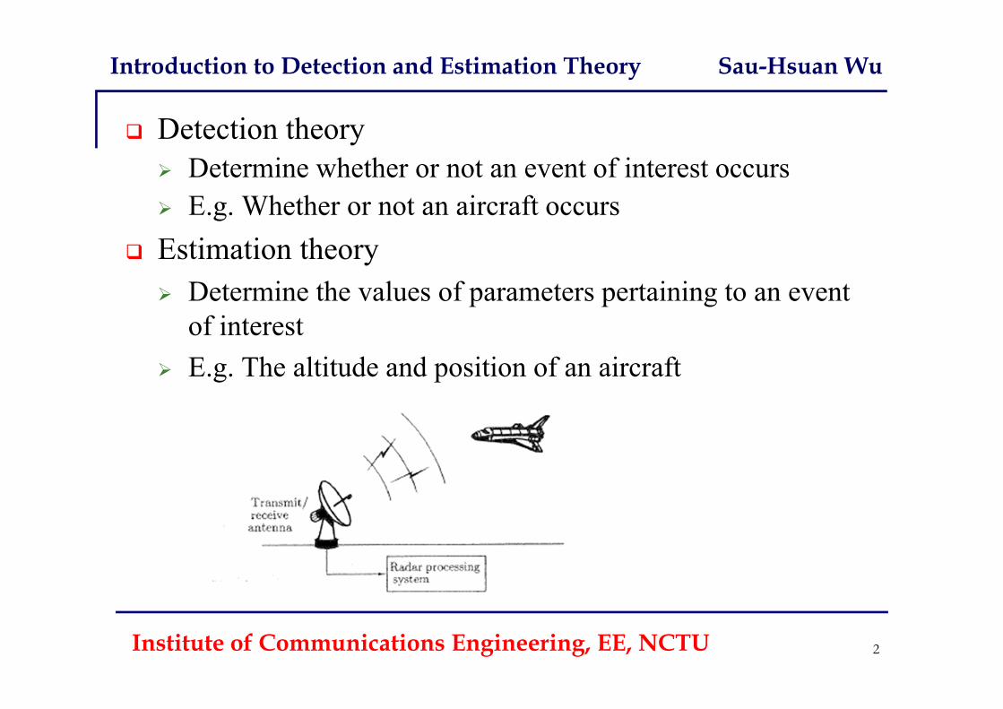
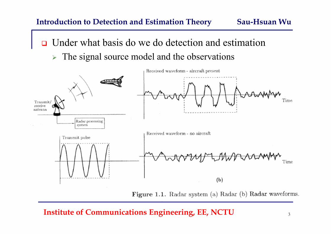
Detection theory Determine whether or not an event of interest occurs E.g. Whether or not an aircraft occurs
Estimation theory Determine the values of parameters pertaining to an event
of interest E.g. The altitude and position of an aircraft
Introduction to Detection and Estimation Theory Sau-Hsuan Wu
Under what basis do we do detection and estimation The signal source model and the observations
Institute of Communications Engineering, EE, NCTU 3
Introduction to Detection and Estimation Theory Sau-Hsuan Wu
Institute of Communications Engineering, EE, NCTU 4
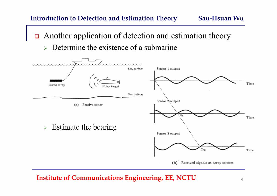
Another application of detection and estimation theory Determine the existence of a submarine
Estimate the bearing
Introduction to Detection and Estimation Theory Sau-Hsuan Wu
Institute of Communications Engineering, EE, NCTU 5
Many more applications Biomedicine: estimate the heart rate or even heart diseases Image analysis: estimate the size, position and orientation of
an object in an image Seismology: estimate the underground distance of an oil
deposit Communications: estimate the signal distortion and
determine the transmitted symbols Economics: estimate the Don-Jones industrial average
Introduction to Detection and Estimation Theory Sau-Hsuan Wu
Institute of Communications Engineering, EE, NCTU 6
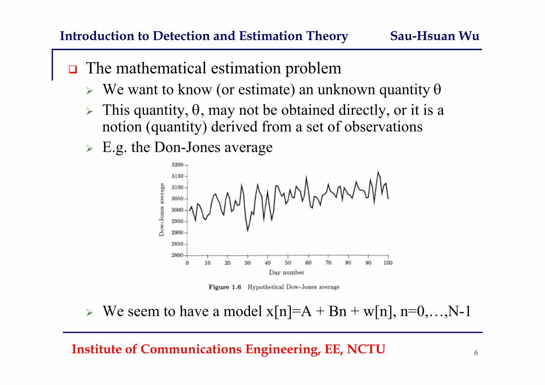
The mathematical estimation problem We want to know (or estimate) an unknown quantity This quantity, , may not be obtained directly, or it is a
notion (quantity) derived from a set of observations E.g. the Don-Jones average
We seem to have a model x[n]=A + Bn + w[n], n=0,…,N-1
Introduction to Detection and Estimation Theory Sau-Hsuan Wu
Institute of Communications Engineering, EE, NCTU 7
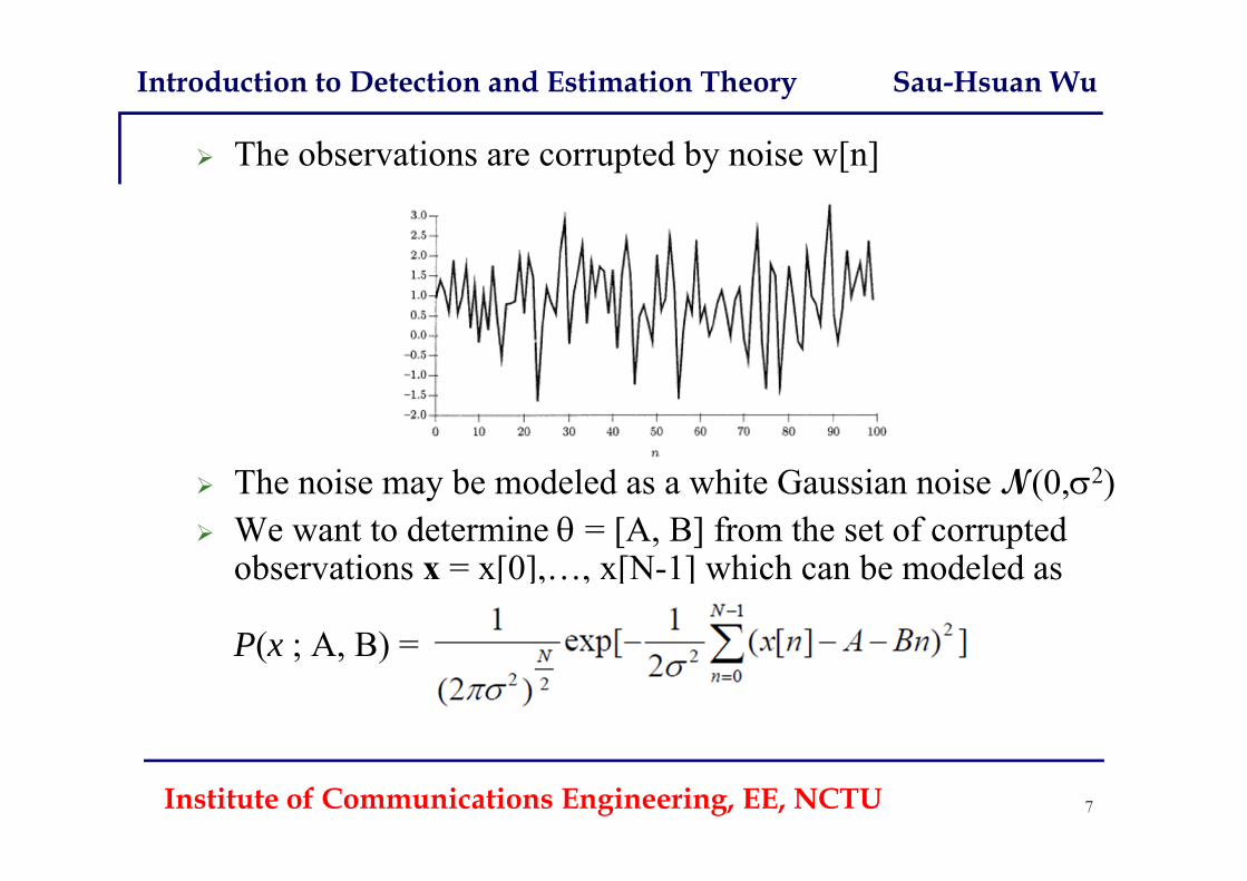
The observations are corrupted by noise w[n]
The noise may be modeled as a white Gaussian noise N(0,2) We want to determine = [A, B] from the set of corrupted
observations x = x[0],…, x[N-1] which can be modeled as
P(x ; A, B) =
Introduction to Detection and Estimation Theory Sau-Hsuan Wu
Our goal is to determine according to the observations, namely Examples:
x[n] = A1 + w[n], n=0,…,N-1 x[n] = A2 + B2 n + w[n], n=0,…,N-1
Â1= x[n]/N and ? Can we try the least square method
How many other kinds of methods can we use Minimum variance unbiased estimator (MVU) Best linear unbiased estimator (BLUE) Maximum likelihood estimator (ML) Bayesian estimator: MMSE, MAP, and …
Institute of Communications Engineering, ECE, NCTU 8
Introduction to Detection and Estimation Theory Sau-Hsuan Wu
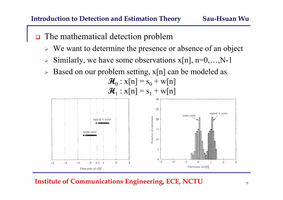
The mathematical detection problem We want to determine the presence or absence of an object Similarly, we have some observations x[n], n=0,…,N-1 Based on our problem setting, x[n] can be modeled as
H0 : x[n] = s0 + w[n]H1 : x[n] = s1 + w[n]
Institute of Communications Engineering, ECE, NCTU 9
Introduction to Detection and Estimation Theory Sau-Hsuan Wu
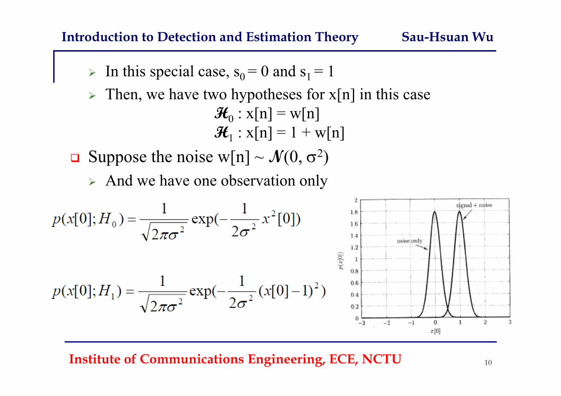
In this special case, s0 = 0 and s1 = 1 Then, we have two hypotheses for x[n] in this case
H0 : x[n] = w[n]H1 : x[n] = 1 + w[n]
Suppose the noise w[n] ~ N(0, 2) And we have one observation only
Institute of Communications Engineering, ECE, NCTU 10
Introduction to Detection and Estimation Theory Sau-Hsuan Wu
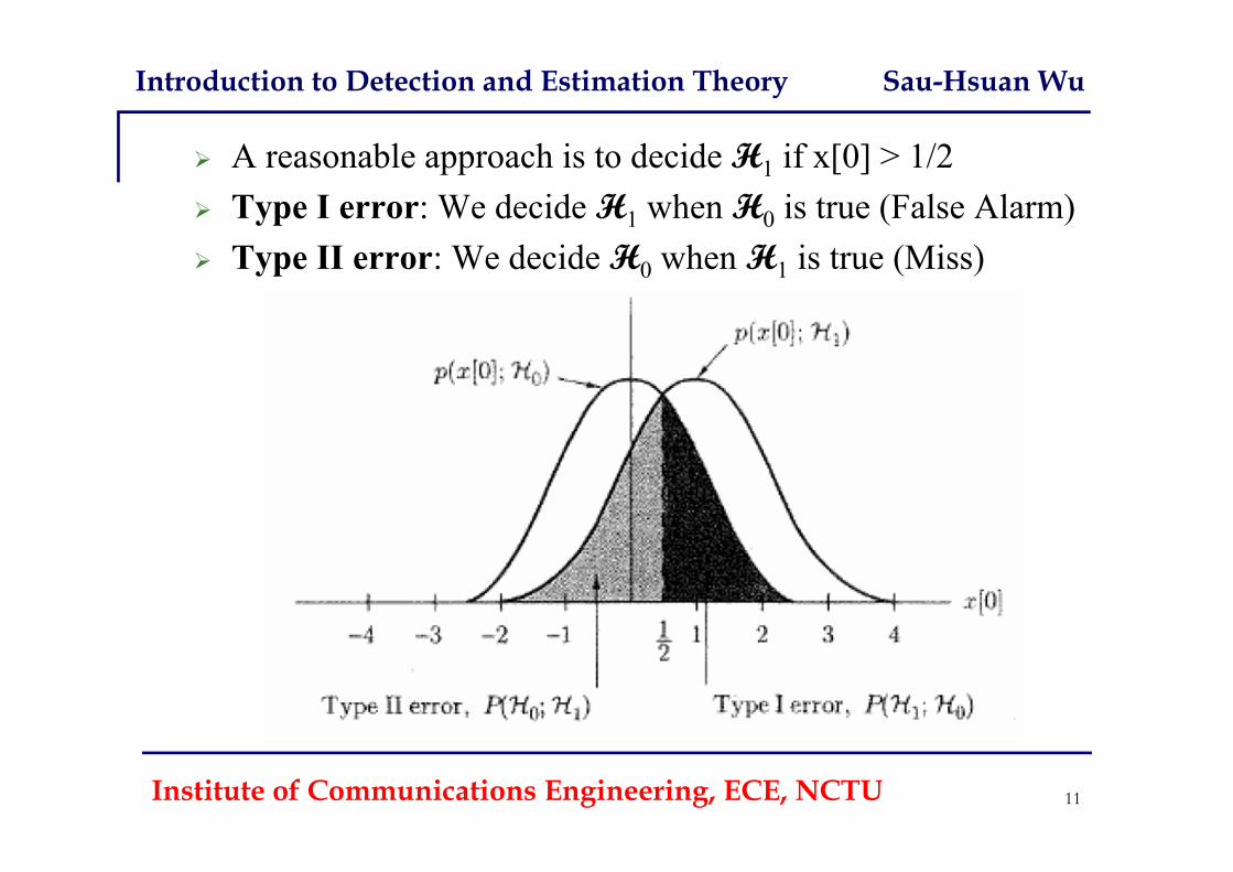
A reasonable approach is to decide H1 if x[0] > 1/2 Type I error: We decide H1 when H0 is true (False Alarm) Type II error: We decide H0 when H1 is true (Miss)
Institute of Communications Engineering, ECE, NCTU 11
Introduction to Detection and Estimation Theory Sau-Hsuan Wu
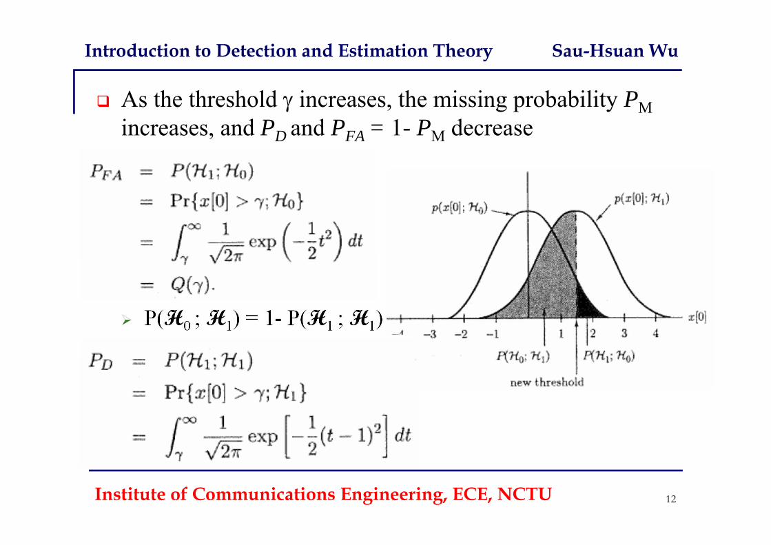
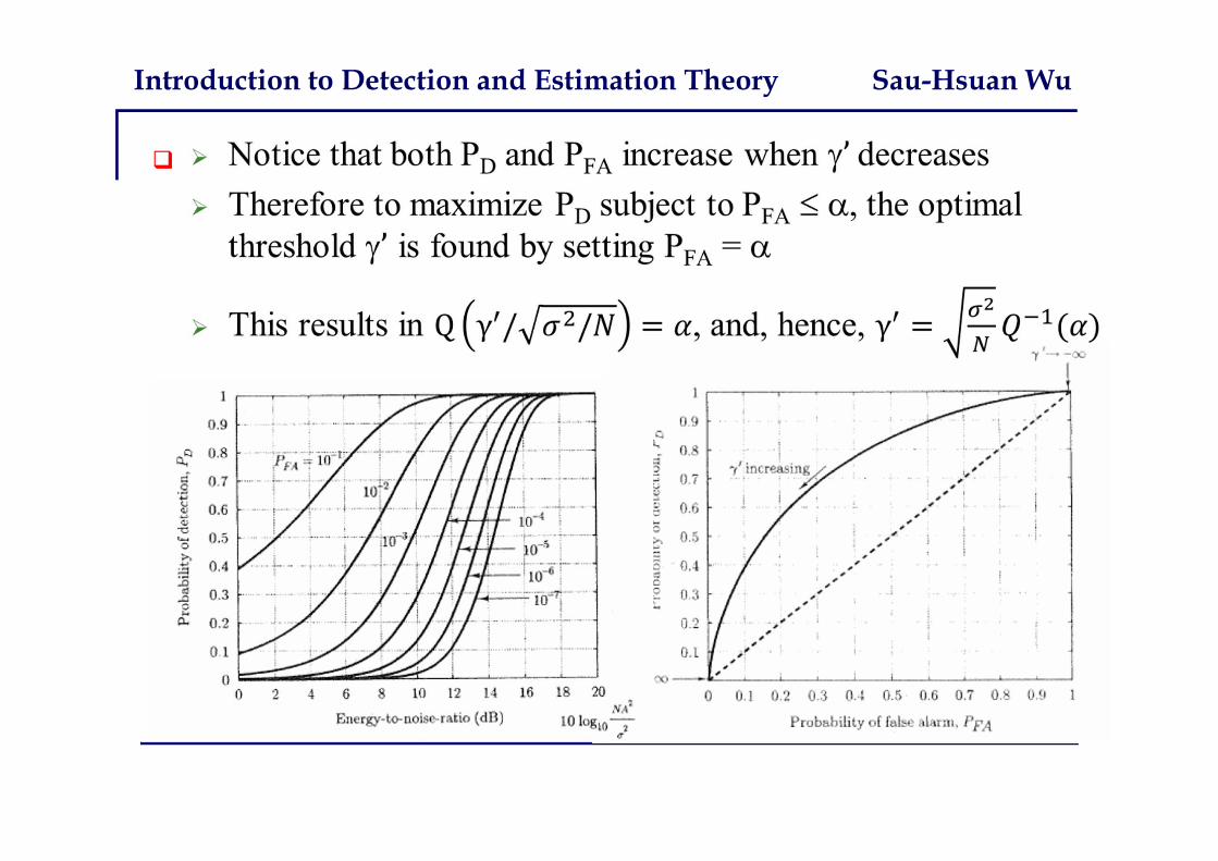
As the threshold increases, the missing probability PMincreases, and PD and PFA = 1- PM decrease
P(H0 ; H1) = 1- P(H1 ; H1)
Institute of Communications Engineering, ECE, NCTU 12
Introduction to Detection and Estimation Theory Sau-Hsuan Wu
In general, we have multiple observations x[n], n=0,…,N-1H0 : x[n] = w[n]H1 : x[n] = A + w[n]
We would decide H1 if T = x[n]/N >
The detection performance increases with d2 = NA2/ 2
Other approach for detection Neyman-Pearson approach
When H0 and H1 are thought of random variables Maximum likelihood (ML) detector Maximum a posterior (MAP) detector Composite hypothesis testing
Institute of Communications Engineering, ECE, NCTU 13
Detection Theory
Institute of Communications Engineering, ECE, NCTU 14
Introduction to Detection and Estimation Theory Sau-Hsuan Wu
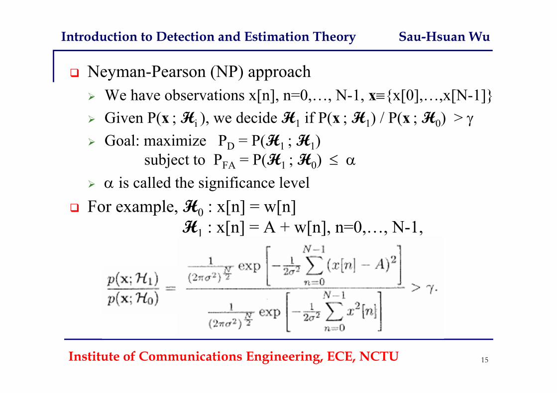
Neyman-Pearson (NP) approach We have observations x[n], n=0,…, N-1, x{x[0],…,x[N-1]} Given P(x ; Hi ), we decide H1 if P(x ; H1) / P(x ; H0) > Goal: maximize PD = P(H1 ; H1)
subject to PFA = P(H1 ; H0) is called the significance level
For example, H0 : x[n] = w[n]H1 : x[n] = A + w[n], n=0,…, N-1,
Institute of Communications Engineering, ECE, NCTU 15
Introduction to Detection and Estimation Theory Sau-Hsuan Wu
Institute of Communications Engineering, ECE, NCTU 16
Introduction to Detection and Estimation Theory Sau-Hsuan Wu
Introduction to Detection and Estimation Theory Sau-Hsuan Wu
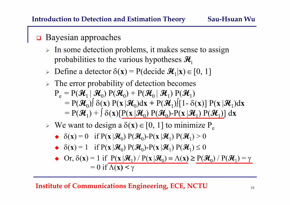
Bayesian approaches In some detection problems, it makes sense to assign
probabilities to the various hypotheses Hi
Define a detector (x) = P(decide H1|x) [0, 1] The error probability of detection becomes
Pe = P(H1 | H0) P(H0) + P(H0 | H1) P(H1)= P(H0) (x) P(x |H0)dx + P(H1)[1- (x)] P(x |H1)dx = P(H1) + (x)[P(x |H0) P(H0)-P(x |H1) P(H1)] dx
We want to design a (x) [0, 1] to minimize Pe (x) = 0 if P(x |H0) P(H0)-P(x |H1) P(H1) > 0 (x) = 1 if P(x |H0) P(H0)-P(x |H1) P(H1) 0 Or, (x) = 1 if P(x |H1) / P(x |H0) (x) P(H0) / P(H1) =
= 0 if (x) <
Institute of Communications Engineering, ECE, NCTU 18
Introduction to Detection and Estimation Theory Sau-Hsuan Wu
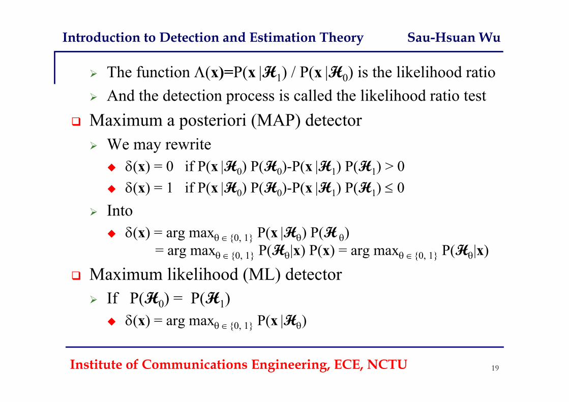
The function (x)=P(x |H1) / P(x |H0) is the likelihood ratio And the detection process is called the likelihood ratio test
Maximum a posteriori (MAP) detector We may rewrite
(x) = 0 if P(x |H0) P(H0)-P(x |H1) P(H1) > 0 (x) = 1 if P(x |H0) P(H0)-P(x |H1) P(H1) 0
Into (x) = arg max {0, 1} P(x |H) P(H )
= arg max {0, 1} P(H|x) P(x) = arg max {0, 1} P(H|x)
Maximum likelihood (ML) detector If P(H0) = P(H1)
(x) = arg max {0, 1} P(x |H)
Institute of Communications Engineering, ECE, NCTU 19
Introduction to Detection and Estimation Theory Sau-Hsuan Wu
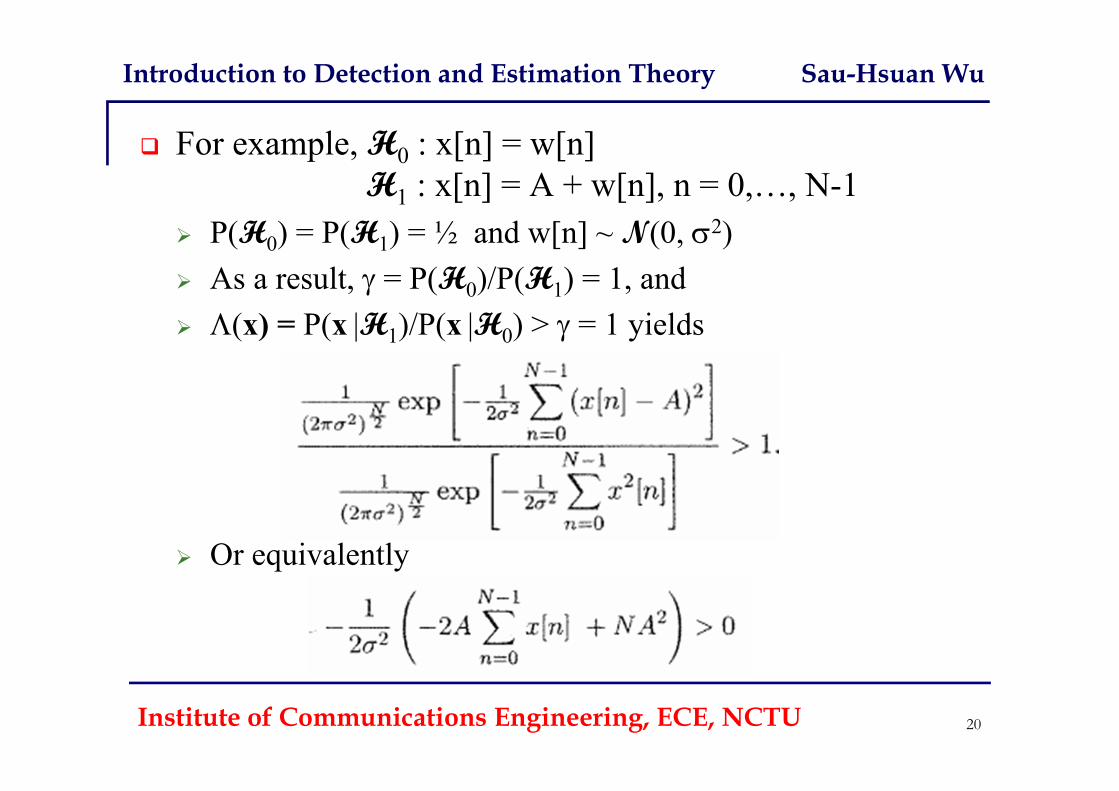
For example, H0 : x[n] = w[n]H1 : x[n] = A + w[n], n = 0,…, N-1
P(H0) = P(H1) = ½ and w[n] ~ N(0, 2) As a result, = P(H0)/P(H1) = 1, and (x) = P(x |H1)/P(x |H0) > = 1 yields
Or equivalently
Institute of Communications Engineering, ECE, NCTU 20
Introduction to Detection and Estimation Theory Sau-Hsuan Wu
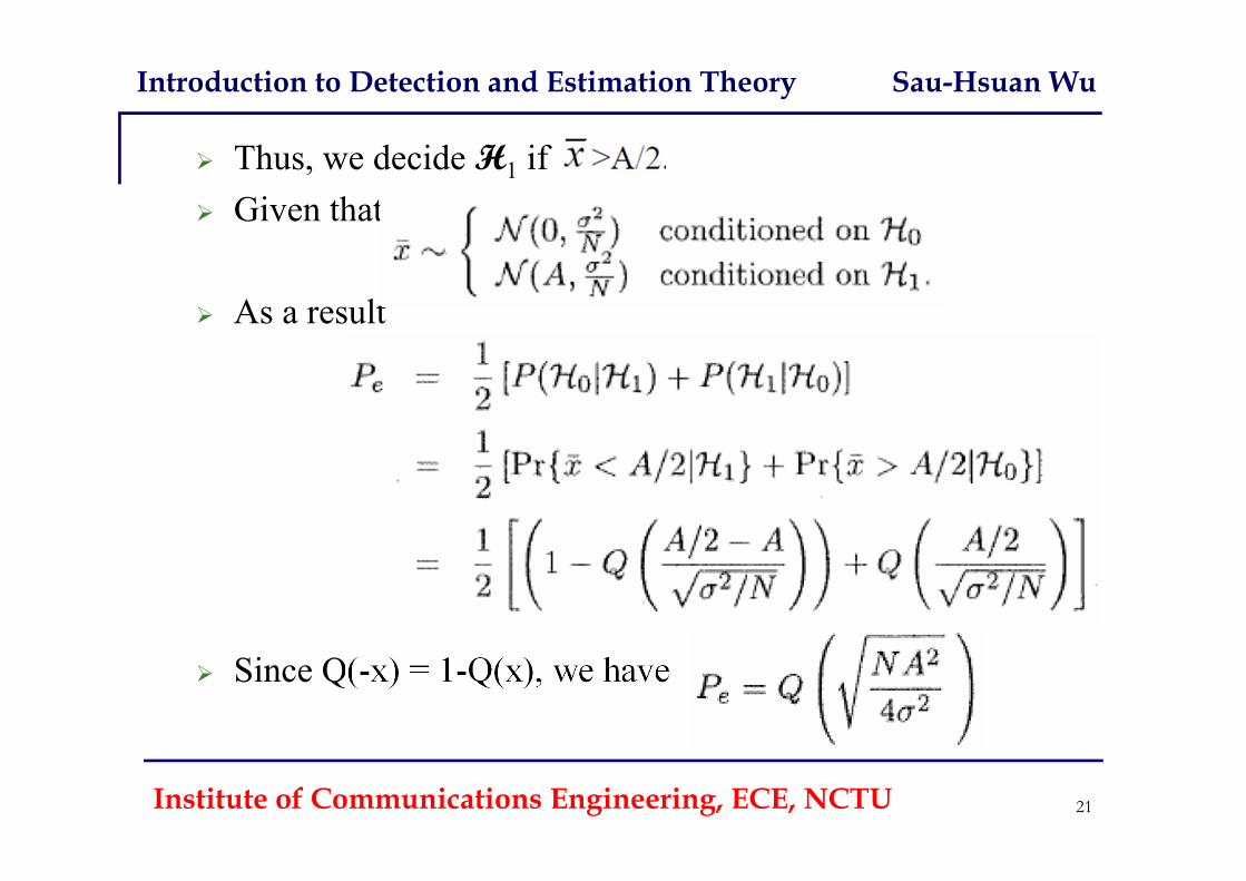
Thus, we decide H1 if Given that
As a result
Since Q(-x) = 1-Q(x), we have
Institute of Communications Engineering, ECE, NCTU 21
Introduction to Detection and Estimation Theory Sau-Hsuan Wu
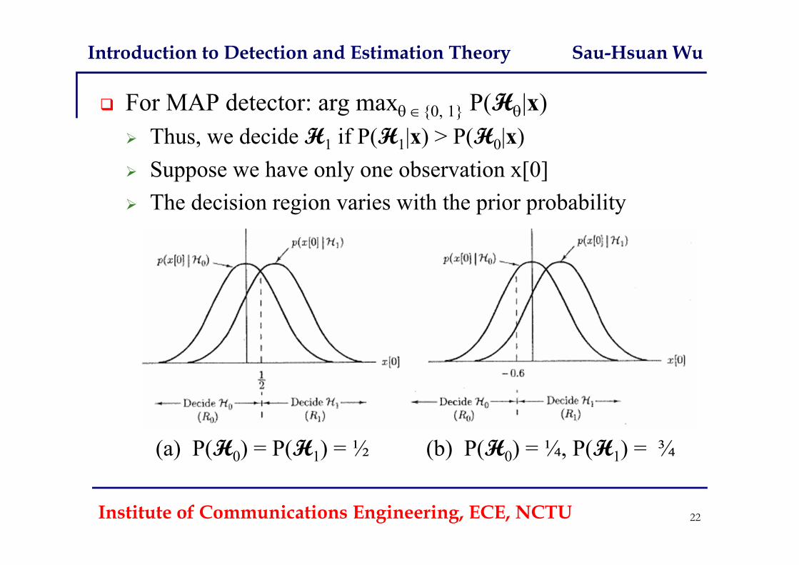
For MAP detector: arg max {0, 1} P(H|x) Thus, we decide H1 if P(H1|x) > P(H0|x) Suppose we have only one observation x[0] The decision region varies with the prior probability
(a) P(H0) = P(H1) = ½ (b) P(H0) = ¼, P(H1) = ¾
Institute of Communications Engineering, ECE, NCTU 22
Introduction to Detection and Estimation Theory Sau-Hsuan Wu
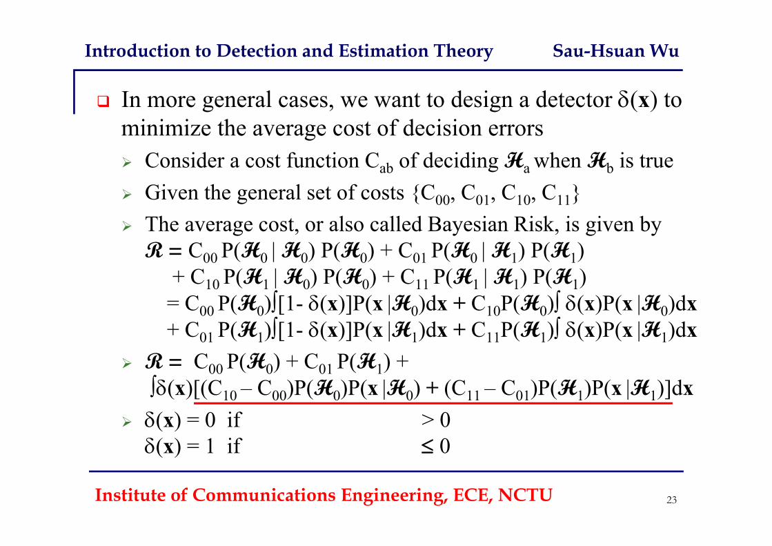
In more general cases, we want to design a detector (x) to minimize the average cost of decision errors Consider a cost function Cab of deciding Ha when Hb is true Given the general set of costs {C00, C01, C10, C11} The average cost, or also called Bayesian Risk, is given by
R = C00 P(H0 | H0) P(H0) + C01 P(H0 | H1) P(H1)+ C10 P(H1 | H0) P(H0) + C11 P(H1 | H1) P(H1)
= C00 P(H0)[1- (x)]P(x |H0)dx + C10P(H0) (x)P(x |H0)dx+ C01 P(H1)[1- (x)]P(x |H1)dx + C11P(H1) (x)P(x |H1)dx
R = C00 P(H0) + C01 P(H1) +(x)[(C10 – C00)P(H0)P(x |H0) + (C11 – C01)P(H1)P(x |H1)]dx
(x) = 0 if > 0(x) = 1 if 0
Institute of Communications Engineering, ECE, NCTU 23
Introduction to Detection and Estimation Theory Sau-Hsuan Wu
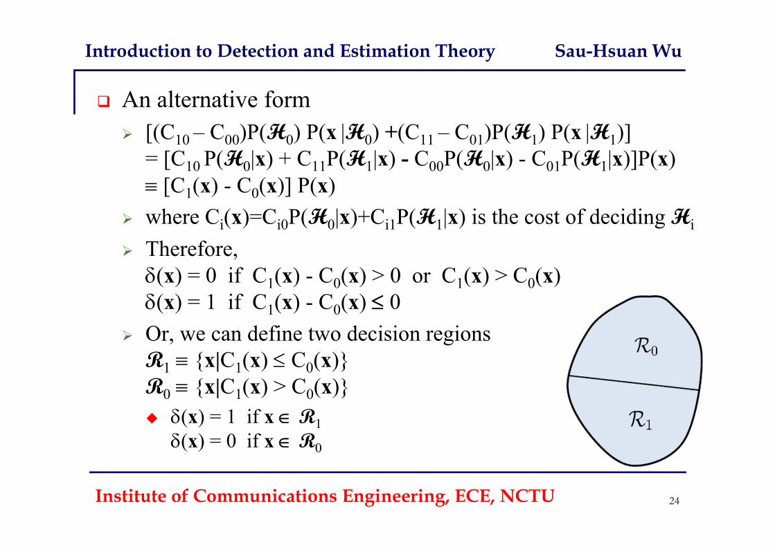
An alternative form [(C10 – C00)P(H0) P(x |H0) +(C11 – C01)P(H1) P(x |H1)]
= [C10 P(H0|x) + C11P(H1|x) - C00P(H0|x) - C01P(H1|x)]P(x) [C1(x) - C0(x)] P(x)
where Ci(x)=Ci0P(H0|x)+Ci1P(H1|x) is the cost of deciding Hi
Therefore, (x) = 0 if C1(x) - C0(x) > 0 or C1(x) > C0(x)(x) = 1 if C1(x) - C0(x) 0
Or, we can define two decision regionsR1 {x|C1(x) C0(x)} R0 {x|C1(x) > C0(x)} (x) = 1 if x R1
(x) = 0 if x R0
Institute of Communications Engineering, ECE, NCTU 24
Introduction to Detection and Estimation Theory Sau-Hsuan Wu
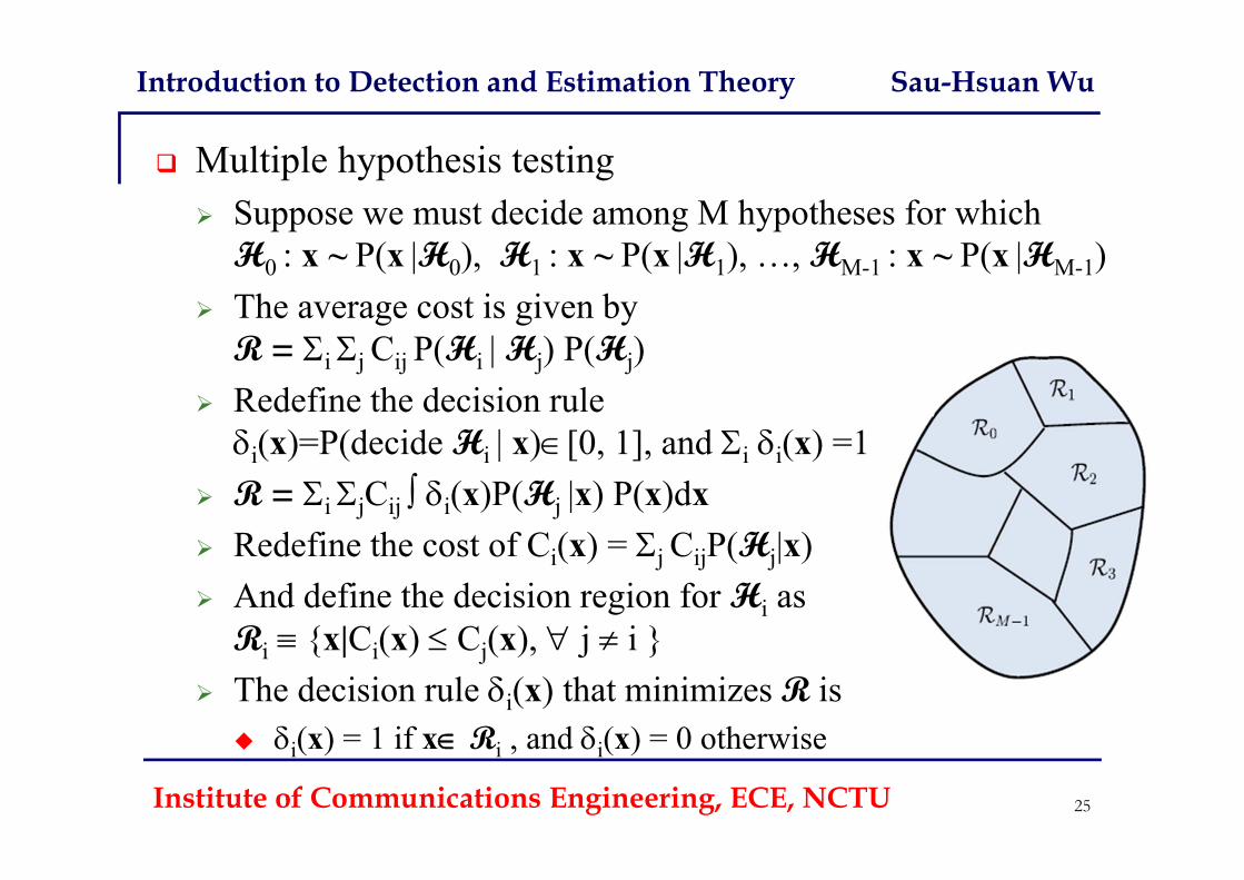
Multiple hypothesis testing Suppose we must decide among M hypotheses for which
H0 : x ~ P(x |H0), H1 : x ~ P(x |H1), …, HM-1 : x ~ P(x |HM-1) The average cost is given by
R = i j Cij P(Hi | Hj) P(Hj) Redefine the decision rule i(x)=P(decide Hi | x)[0, 1], and i i(x) =1
R = i jCij i(x)P(Hj |x) P(x)dx Redefine the cost of Ci(x) = j CijP(Hj|x) And define the decision region for Hi as
Ri {x|Ci(x) Cj(x), j i } The decision rule i(x) that minimizes R is
i(x) = 1 if x Ri , and i(x) = 0 otherwise
Institute of Communications Engineering, ECE, NCTU 25
Estimation Theory
Institute of Communications Engineering, ECE, NCTU 26
Introduction to Detection and Estimation Theory Sau-Hsuan Wu
Institute of Communications Engineering, EE, NCTU 27
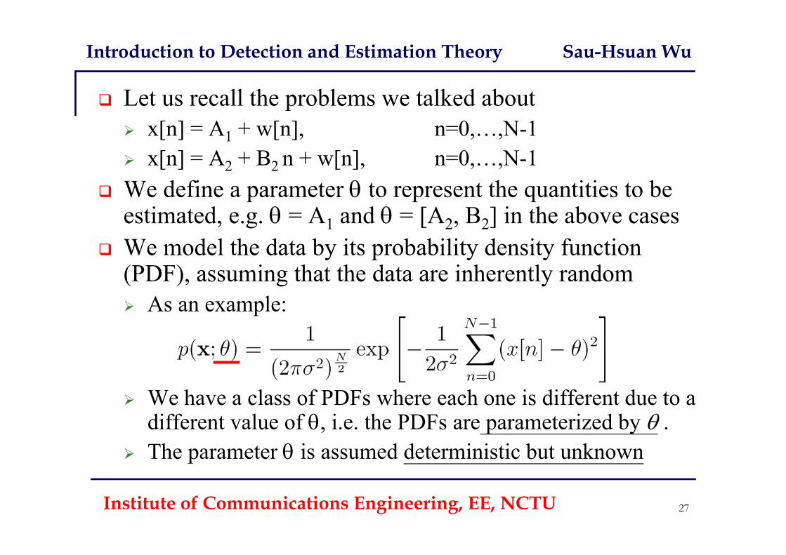
Let us recall the problems we talked about x[n] = A1 + w[n], n=0,…,N-1 x[n] = A2 + B2 n + w[n], n=0,…,N-1
We define a parameter to represent the quantities to be estimated, e.g. = A1 and = [A2, B2] in the above cases
We model the data by its probability density function (PDF), assuming that the data are inherently random As an example:
We have a class of PDFs where each one is different due to a different value of , i.e. the PDFs are parameterized by .
The parameter is assumed deterministic but unknown
Introduction to Detection and Estimation Theory Sau-Hsuan Wu
Institute of Communications Engineering, EE, NCTU 28
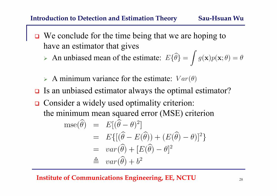
We conclude for the time being that we are hoping to have an estimator that gives An unbiased mean of the estimate:
A minimum variance for the estimate: Is an unbiased estimator always the optimal estimator? Consider a widely used optimality criterion:
the minimum mean squared error (MSE) criterion
Introduction to Detection and Estimation Theory Sau-Hsuan Wu
Institute of Communications Engineering, EE, NCTU 29
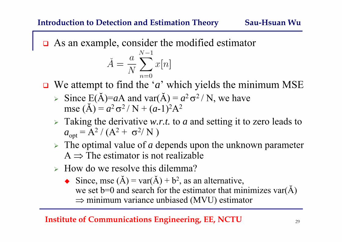
As an example, consider the modified estimator
We attempt to find the ‘a’ which yields the minimum MSE Since E(Ă)=aA and var(Ă) = a2 2 / N, we have
mse (Ă) = a2 2 / N + (a-1)2A2
Taking the derivative w.r.t. to a and setting it to zero leads toaopt = A2 / (A2 + 2/ N )
The optimal value of a depends upon the unknown parameter A The estimator is not realizable
How do we resolve this dilemma? Since, mse (Ă) = var(Ă) + b2, as an alternative,
we set b=0 and search for the estimator that minimizes var(Ă) minimum variance unbiased (MVU) estimator
Introduction to Detection and Estimation Theory Sau-Hsuan Wu
Institute of Communications Engineering, EE, NCTU 30
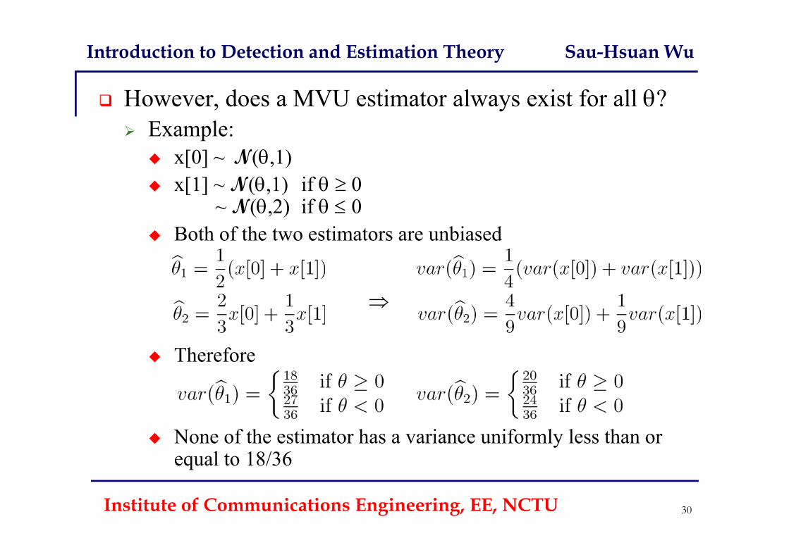
However, does a MVU estimator always exist for all ? Example:
x[0] ~ N(,1) x[1] ~ N(,1) if 0
~ N(,2) if 0 Both of the two estimators are unbiased
Therefore
None of the estimator has a variance uniformly less than or equal to 18/36
Introduction to Detection and Estimation Theory Sau-Hsuan Wu
Institute of Communications Engineering, EE, NCTU 31
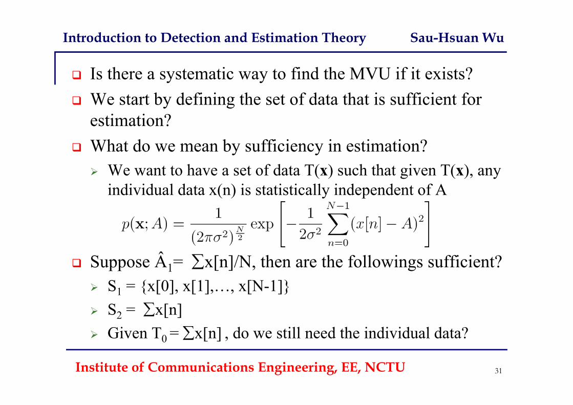
Is there a systematic way to find the MVU if it exists? We start by defining the set of data that is sufficient for
estimation? What do we mean by sufficiency in estimation? We want to have a set of data T(x) such that given T(x), any
individual data x(n) is statistically independent of A
Suppose Â1= x[n]/N, then are the followings sufficient? S1 = {x[0], x[1],…, x[N-1]} S2 = x[n] GivenT0 = x[n] , do we still need the individual data?
Introduction to Detection and Estimation Theory Sau-Hsuan Wu
Institute of Communications Engineering, EE, NCTU 32
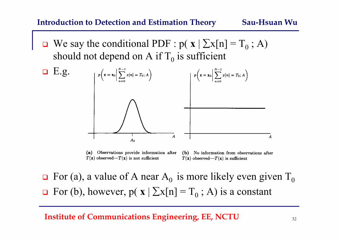
We say the conditional PDF : p( x | x[n] = T0 ; A) should not depend on A if T0 is sufficient
E.g.
For (a), a value of A near A0 is more likely even given T0
For (b), however, p( x | x[n] = T0 ; A) is a constant
Introduction to Detection and Estimation Theory Sau-Hsuan Wu
Institute of Communications Engineering, EE, NCTU 33
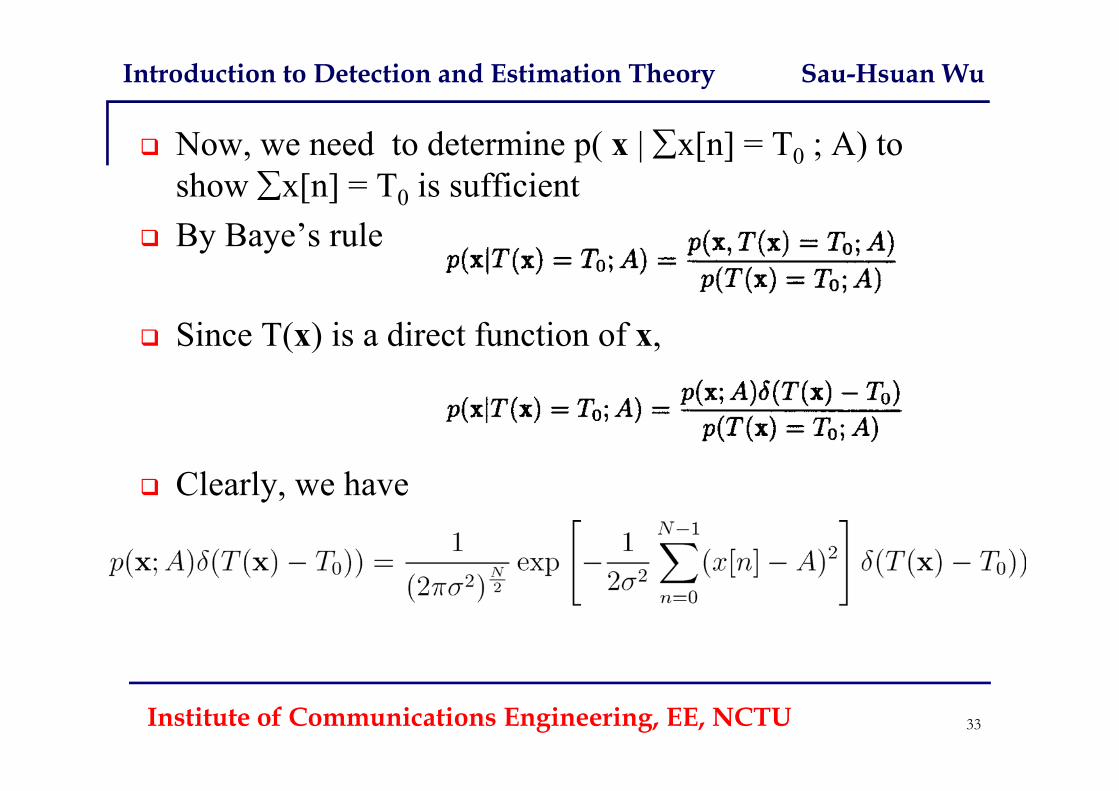
Now, we need to determine p( x | x[n] = T0 ; A) to show x[n] = T0 is sufficient
By Baye’s rule
Since T(x) is a direct function of x,
Clearly, we have
Introduction to Detection and Estimation Theory Sau-Hsuan Wu
Institute of Communications Engineering, EE, NCTU 34
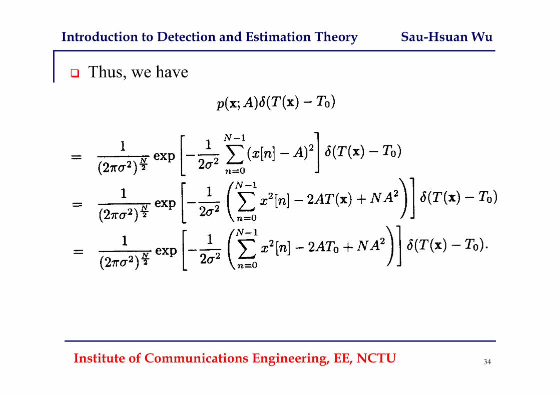
Thus, we have
Introduction to Detection and Estimation Theory Sau-Hsuan Wu
Institute of Communications Engineering, EE, NCTU 35
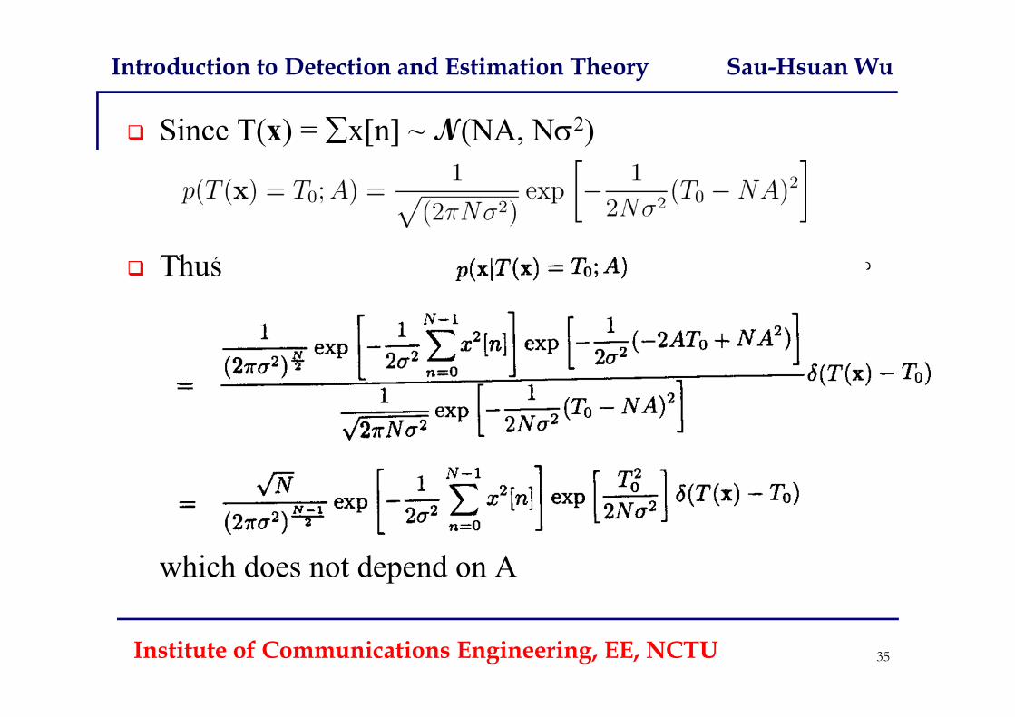
Since T(x) = x[n] ~ N(NA, N2)
Thus
which does not depend on A
Introduction to Detection and Estimation Theory Sau-Hsuan Wu
Institute of Communications Engineering, EE, NCTU 36
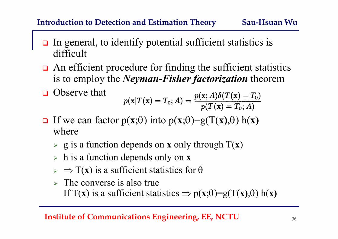
In general, to identify potential sufficient statistics is difficult
An efficient procedure for finding the sufficient statistics is to employ the Neyman-Fisher factorization theorem
Observe that
If we can factor p(x;) into p(x;)=g(T(x),) h(x)where g is a function depends on x only through T(x) h is a function depends only on x T(x) is a sufficient statistics for The converse is also true
If T(x) is a sufficient statistics p(x;)=g(T(x),) h(x)
Introduction to Detection and Estimation Theory Sau-Hsuan Wu
Institute of Communications Engineering, EE, NCTU 37
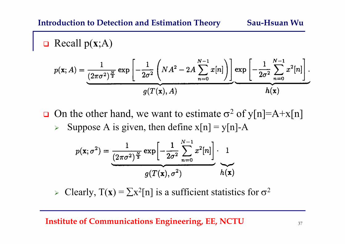
Recall p(x;A)
On the other hand, we want to estimate 2 of y[n]=A+x[n] Suppose A is given, then define x[n] = y[n]-A
Clearly, T(x) = x2[n] is a sufficient statistics for 2
Introduction to Detection and Estimation Theory Sau-Hsuan Wu
Institute of Communications Engineering, EE, NCTU 38
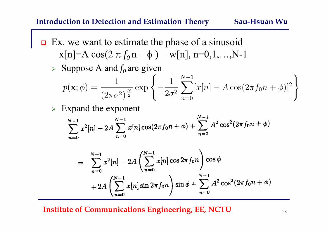
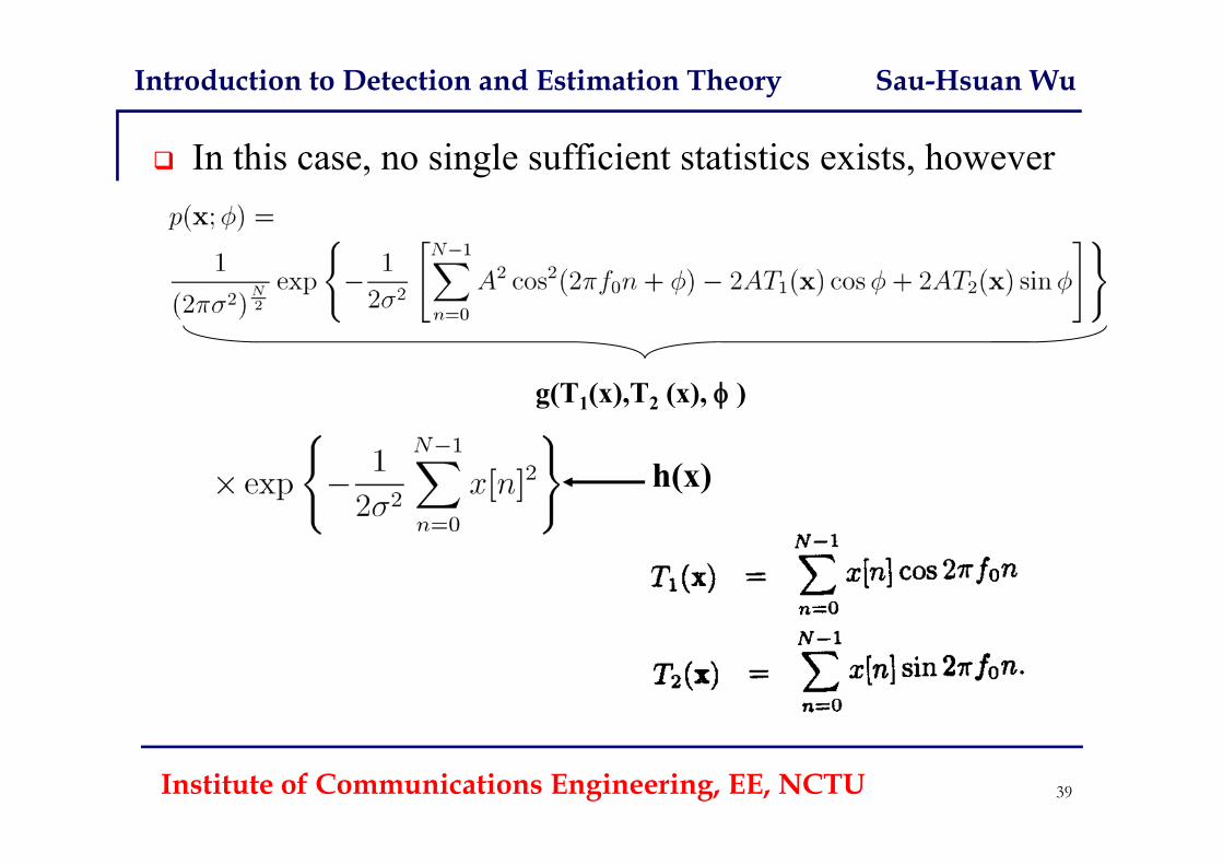
Ex. we want to estimate the phase of a sinusoidx[n]=A cos(2 f0 n + ) + w[n], n=0,1,…,N-1
Suppose A and f0 are given
Expand the exponent
Introduction to Detection and Estimation Theory Sau-Hsuan Wu
Institute of Communications Engineering, EE, NCTU 39
In this case, no single sufficient statistics exists, however
g(T1(x),T2 (x), )
h(x)
Introduction to Detection and Estimation Theory Sau-Hsuan Wu
Institute of Communications Engineering, EE, NCTU 40
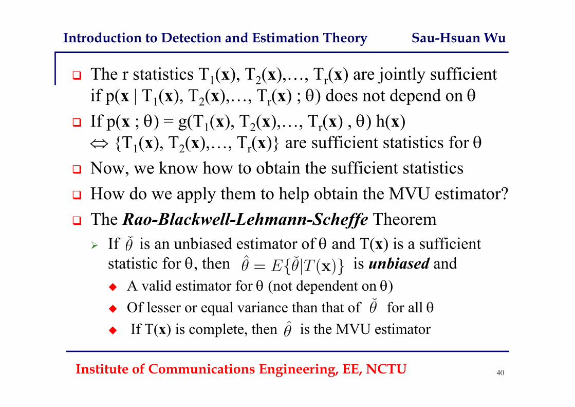
The r statistics T1(x), T2(x),…, Tr(x) are jointly sufficient if p(x | T1(x), T2(x),…, Tr(x) ; ) does not depend on
If p(x ; ) = g(T1(x), T2(x),…, Tr(x) , ) h(x) {T1(x), T2(x),…, Tr(x)} are sufficient statistics for
Now, we know how to obtain the sufficient statistics How do we apply them to help obtain the MVU estimator? The Rao-Blackwell-Lehmann-Scheffe Theorem If is an unbiased estimator of and T(x) is a sufficient
statistic for , then is unbiased and A valid estimator for (not dependent on ) Of lesser or equal variance than that of for all If T(x) is complete, then is the MVU estimator
Introduction to Detection and Estimation Theory Sau-Hsuan Wu
Institute of Communications Engineering, EE, NCTU 41
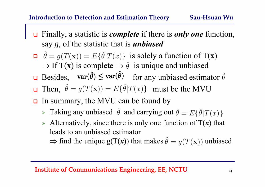
Finally, a statistic is complete if there is only one function, say g, of the statistic that is unbiased
is solely a function of T(x) If T(x) is complete is unique and unbiased
Besides, for any unbiased estimator Then, must be the MVU In summary, the MVU can be found by Taking any unbiased and carrying out Alternatively, since there is only one function of T(x) that
leads to an unbiased estimator find the unique g(T(x)) that makes unbiased
Introduction to Detection and Estimation Theory Sau-Hsuan Wu
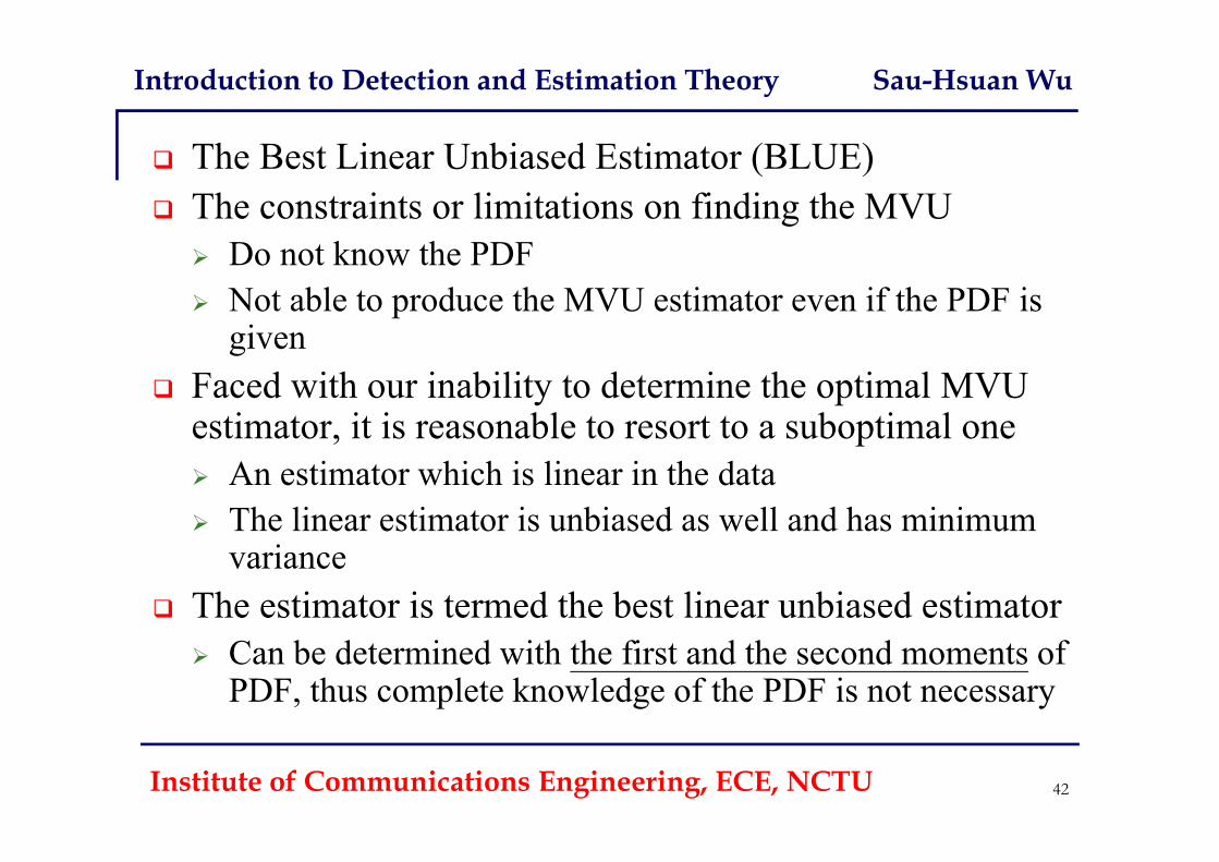
The Best Linear Unbiased Estimator (BLUE) The constraints or limitations on finding the MVU Do not know the PDF Not able to produce the MVU estimator even if the PDF is
given Faced with our inability to determine the optimal MVU
estimator, it is reasonable to resort to a suboptimal one An estimator which is linear in the data The linear estimator is unbiased as well and has minimum
variance The estimator is termed the best linear unbiased estimator Can be determined with the first and the second moments of
PDF, thus complete knowledge of the PDF is not necessary
Institute of Communications Engineering, ECE, NCTU 42
Introduction to Detection and Estimation Theory Sau-Hsuan Wu
Institute of Communications Engineering, EE, NCTU 43
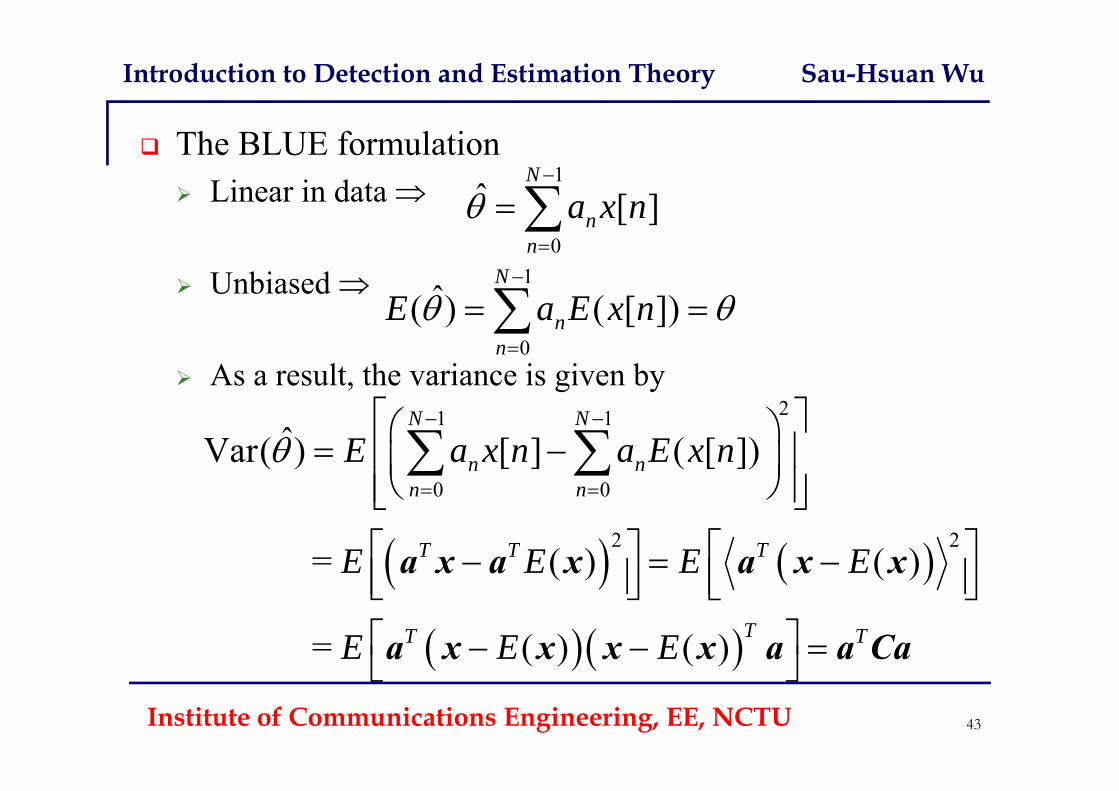
The BLUE formulation Linear in data
Unbiased
As a result, the variance is given by
1
0
ˆ [ ]N
nn
a x n
1
0
ˆ( ) ( [ ])N
nn
E a E x n
21 1
0 0
22
ˆVar( ) [ ] ( [ ])
= ( ) ( )
= ( ) ( )
N N
n nn n
T T T
TT T
E a x n a E x n
E E E E
E E E
a x a x a x x
a x x x x a a Ca
Introduction to Detection and Estimation Theory Sau-Hsuan Wu
Institute of Communications Engineering, EE, NCTU 44
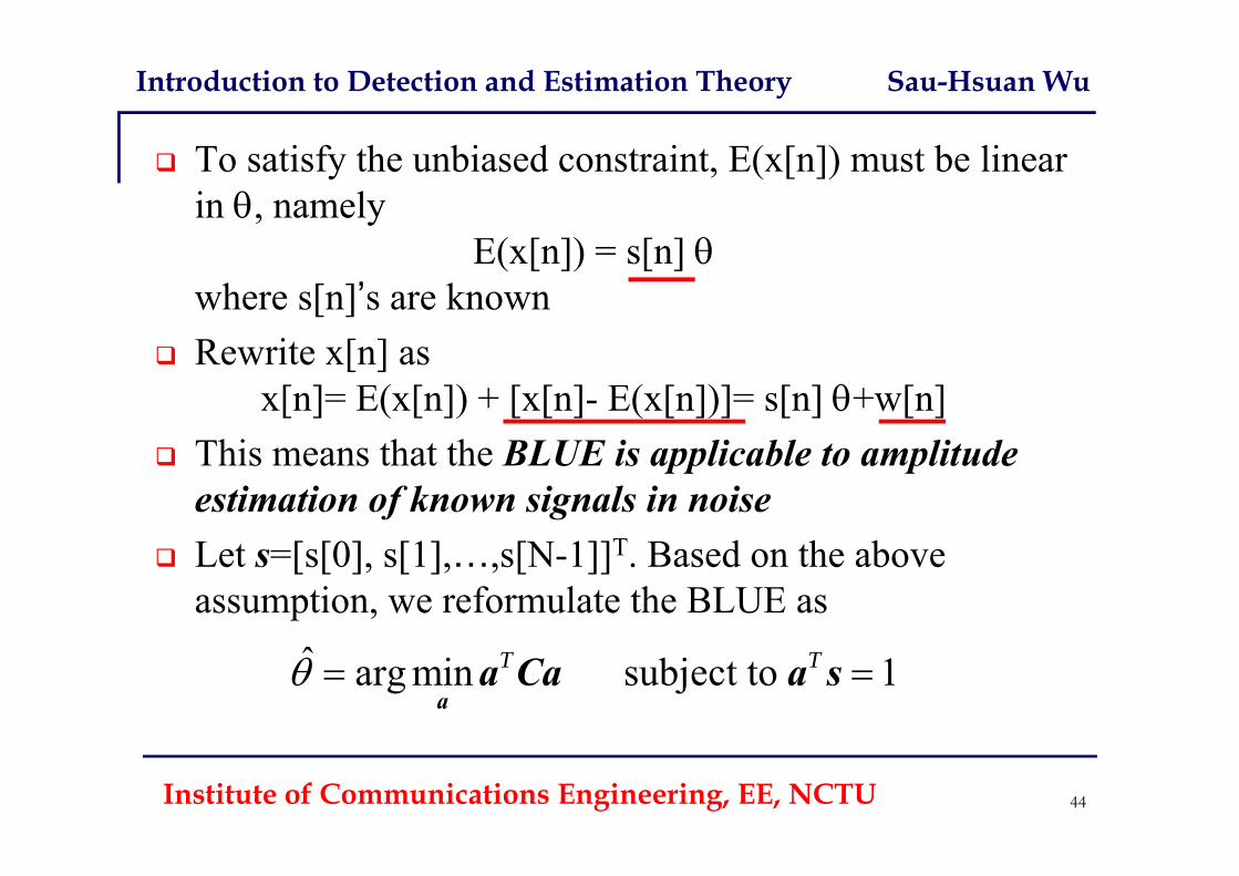
To satisfy the unbiased constraint, E(x[n]) must be linear in , namely
E(x[n]) = s[n] where s[n]’s are known
Rewrite x[n] as x[n]= E(x[n]) + [x[n]- E(x[n])]= s[n] +w[n]
This means that the BLUE is applicable to amplitude estimation of known signals in noise
Let s=[s[0], s[1],…,s[N-1]]T. Based on the above assumption, we reformulate the BLUE as
ˆ arg min subject to 1T T a
a Ca a s
Introduction to Detection and Estimation Theory Sau-Hsuan Wu
Institute of Communications Engineering, EE, NCTU 45
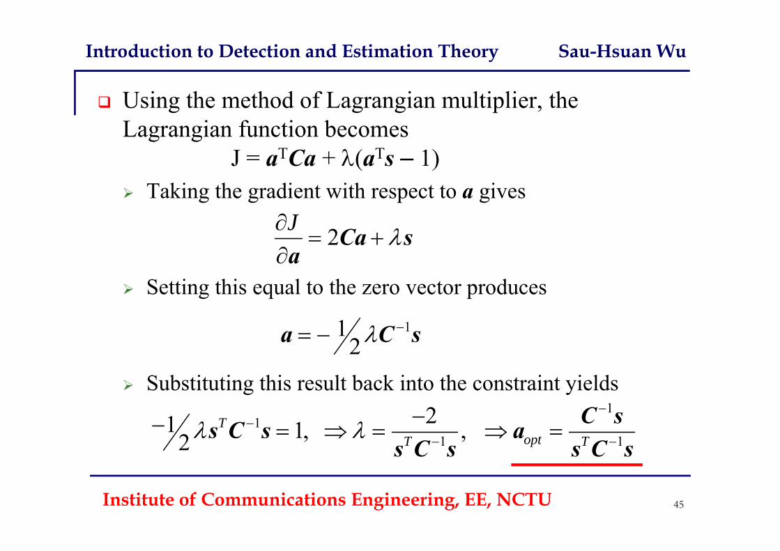
Using the method of Lagrangian multiplier, the Lagrangian function becomes
J = aTCa + (aTs – 1) Taking the gradient with respect to a gives
Setting this equal to the zero vector produces
Substituting this result back into the constraint yields
2J
Ca s
a
112
a C s
11
1 121 1, , 2
ToptT T
C ss C s a
s C s s C s
Introduction to Detection and Estimation Theory Sau-Hsuan Wu
Institute of Communications Engineering, EE, NCTU 46
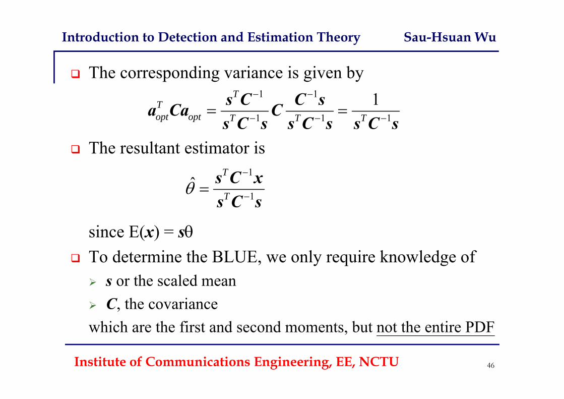
The corresponding variance is given by
The resultant estimator is
since E(x) = s To determine the BLUE, we only require knowledge of s or the scaled mean C, the covariancewhich are the first and second moments, but not the entire PDF
1 1
1 1 11T
Topt opt T T T
s C C sa Ca Cs C s s C s s C s
1
1ˆ
T
T
s C xs C s
Introduction to Detection and Estimation Theory Sau-Hsuan Wu
Institute of Communications Engineering, EE, NCTU 47
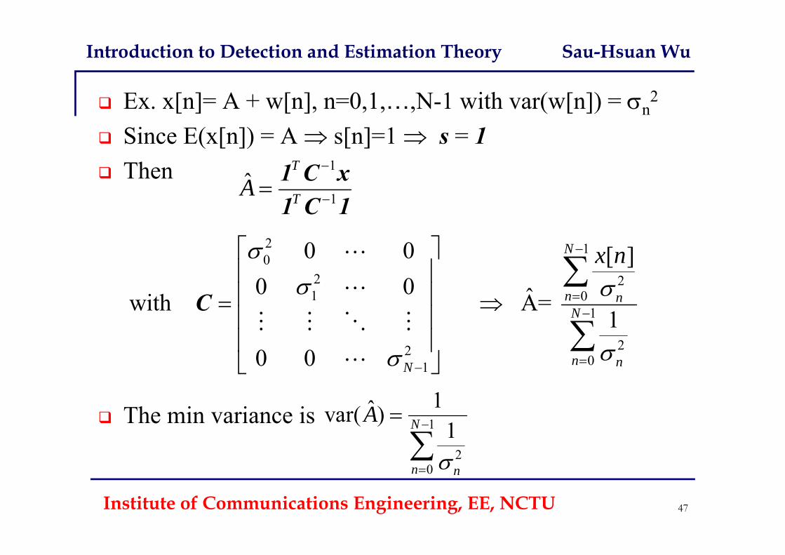
Ex. x[n]= A + w[n], n=0,1,…,N-1 with var(w[n]) = n2
Since E(x[n]) = A s[n]=1 s = 1 Then
The min variance is
1
1ˆ
T
TA
1 C x1 C 1
1
20
1ˆvar( )1N
n n
A
2 10
2 21 0
1
2201
0 0 [ ]0 0 ˆwith A=
10 0
N
n nN
n nN
x n
C
Introduction to Detection and Estimation Theory Sau-Hsuan Wu
48Institute of Communications Engineering, EE, NCTU
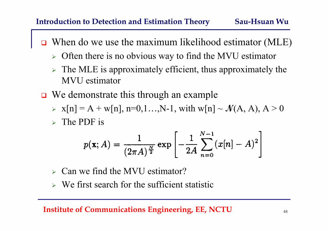
When do we use the maximum likelihood estimator (MLE) Often there is no obvious way to find the MVU estimator The MLE is approximately efficient, thus approximately the
MVU estimator We demonstrate this through an example x[n] = A + w[n], n=0,1…,N-1, with w[n] ~ N(A, A), A > 0 The PDF is
Can we find the MVU estimator? We first search for the sufficient statistic
Introduction to Detection and Estimation Theory Sau-Hsuan Wu
49Institute of Communications Engineering, EE, NCTU
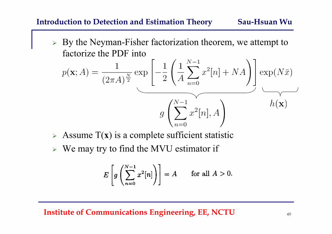
By the Neyman-Fisher factorization theorem, we attempt to factorize the PDF into
Assume T(x) is a complete sufficient statistic We may try to find the MVU estimator if
Introduction to Detection and Estimation Theory Sau-Hsuan Wu
50Institute of Communications Engineering, EE, NCTU
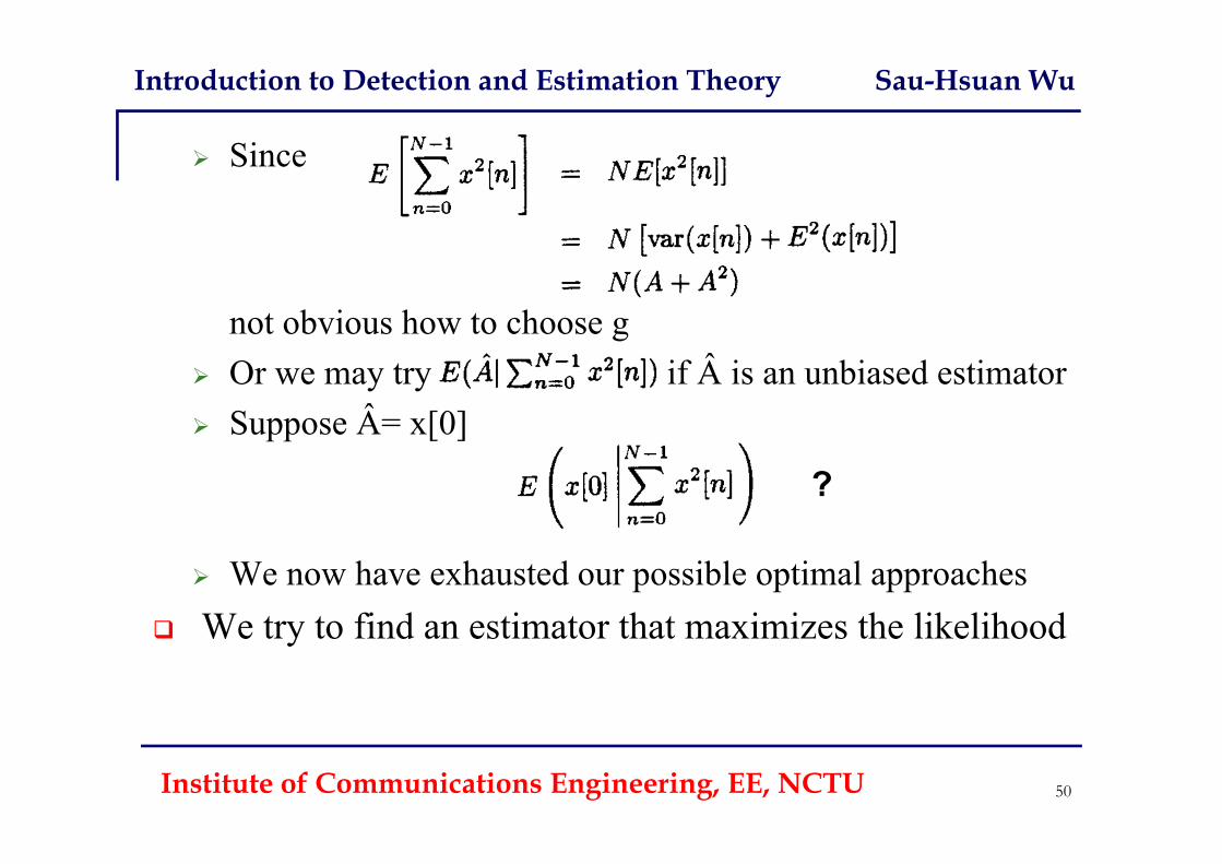
Since
not obvious how to choose g Or we may try if  is an unbiased estimator Suppose Â= x[0]
We now have exhausted our possible optimal approaches We try to find an estimator that maximizes the likelihood
?
Introduction to Detection and Estimation Theory Sau-Hsuan Wu
51Institute of Communications Engineering, EE, NCTU
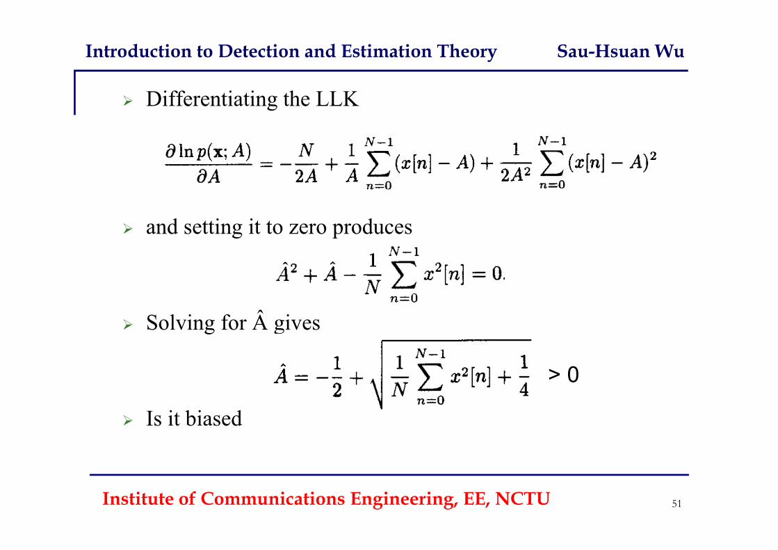
Differentiating the LLK
and setting it to zero produces
Solving for  gives
Is it biased
> 0
Introduction to Detection and Estimation Theory Sau-Hsuan Wu
52Institute of Communications Engineering, EE, NCTU
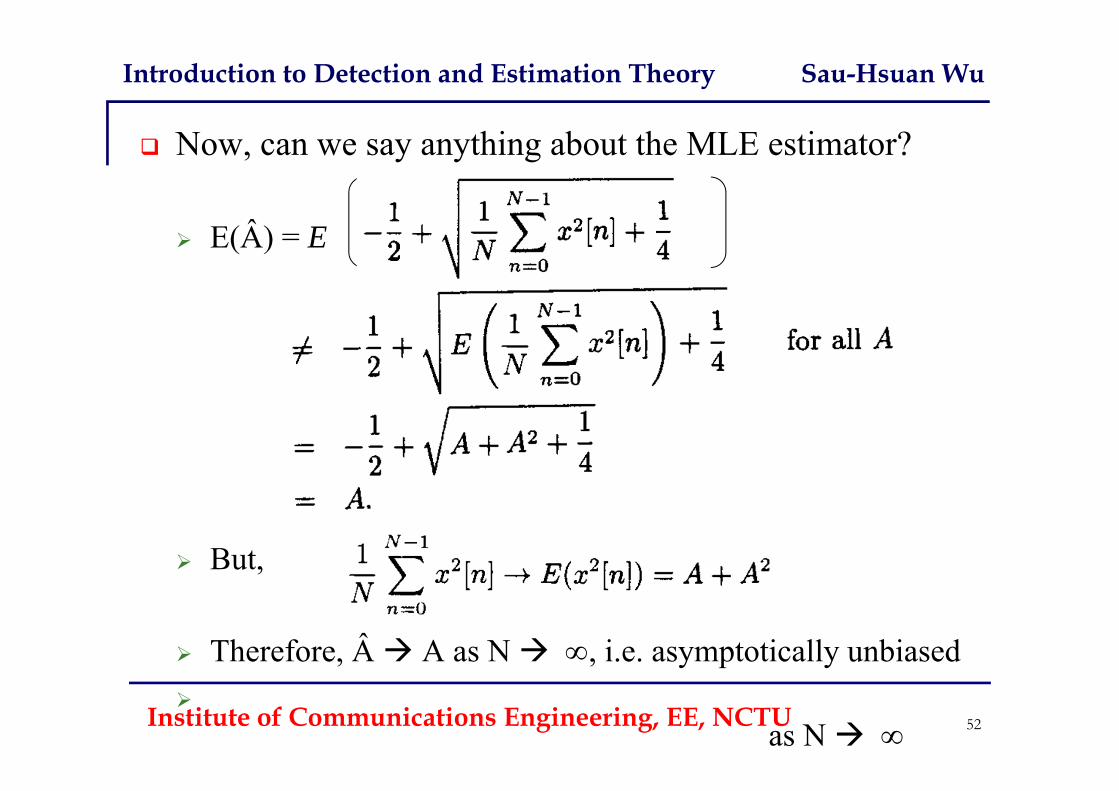
Now, can we say anything about the MLE estimator?
E(Â) = E
But,
Therefore, Â A as N , i.e. asymptotically unbiased
as N
The Bayesian Philosophy and General Estimators
Institute of Communications Engineering, ECE, NCTU 53
Introduction to Detection and Estimation Theory Sau-Hsuan Wu
Institute of Communications Engineering, EE, NCTU 54
Note: In an actual problem, we are not given a PDF but must choose one that is not only consistent with the problem constraints and any prior knowledge, but one that is also mathematically tractable
Sometimes, we might want to constraint the estimator to produce values in a certain range. To incorporate this prior knowledge, we can assume that
is no longer deterministic but a random variable having a uniform distribution over the [-U, U] interval for instance
Assign a PDF to , then the data are described by the joint PDF
Any estimator that yields estimates according to the prior knowledge of is termed a Bayesian estimator
Introduction to Detection and Estimation Theory Sau-Hsuan Wu
Institute of Communications Engineering, EE, NCTU
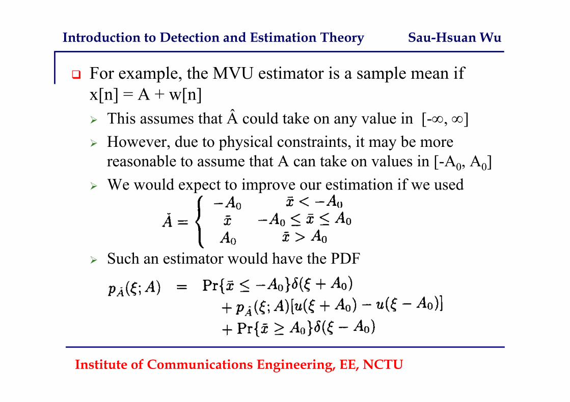
For example, the MVU estimator is a sample mean if x[n] = A + w[n] This assumes that  could take on any value in [-, ] However, due to physical constraints, it may be more
reasonable to assume that A can take on values in [-A0, A0] We would expect to improve our estimation if we used
Such an estimator would have the PDF
Introduction to Detection and Estimation Theory Sau-Hsuan Wu
Institute of Communications Engineering, EE, NCTU
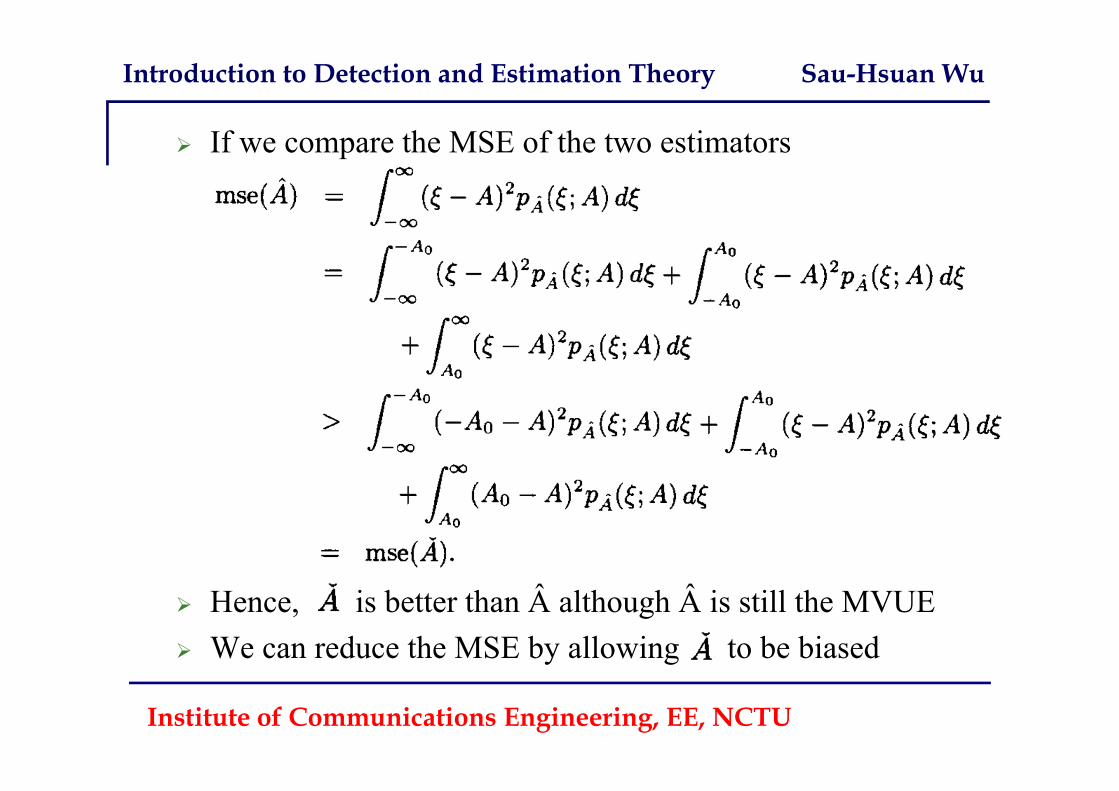
If we compare the MSE of the two estimators
Hence, is better than  although  is still the MVUE We can reduce the MSE by allowing to be biased
Introduction to Detection and Estimation Theory Sau-Hsuan Wu
Institute of Communications Engineering, EE, NCTU
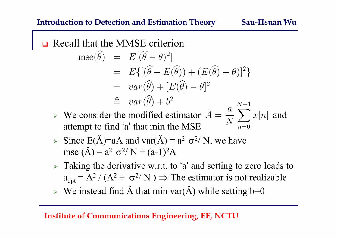
Recall that the MMSE criterion
We consider the modified estimator and attempt to find ‘a’ that min the MSE
Since E(Ă)=aA and var(Ă) = a2 2/ N, we havemse (Ă) = a2 2/ N + (a-1)2A
Taking the derivative w.r.t. to ‘a’ and setting to zero leads toaopt = A2 / (A2 + 2/ N ) The estimator is not realizable
We instead find  that min var(Â) while setting b=0
Introduction to Detection and Estimation Theory Sau-Hsuan Wu
Institute of Communications Engineering, EE, NCTU
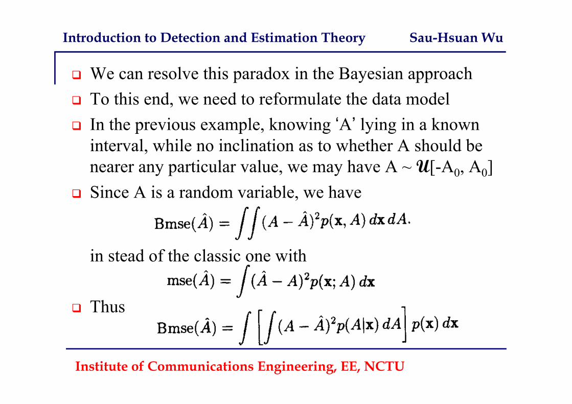
We can resolve this paradox in the Bayesian approach To this end, we need to reformulate the data model In the previous example, knowing ‘A’ lying in a known
interval, while no inclination as to whether A should be nearer any particular value, we may have A ~ U[-A0, A0]
Since A is a random variable, we have
in stead of the classic one with
Thus
Introduction to Detection and Estimation Theory Sau-Hsuan Wu
Institute of Communications Engineering, EE, NCTU
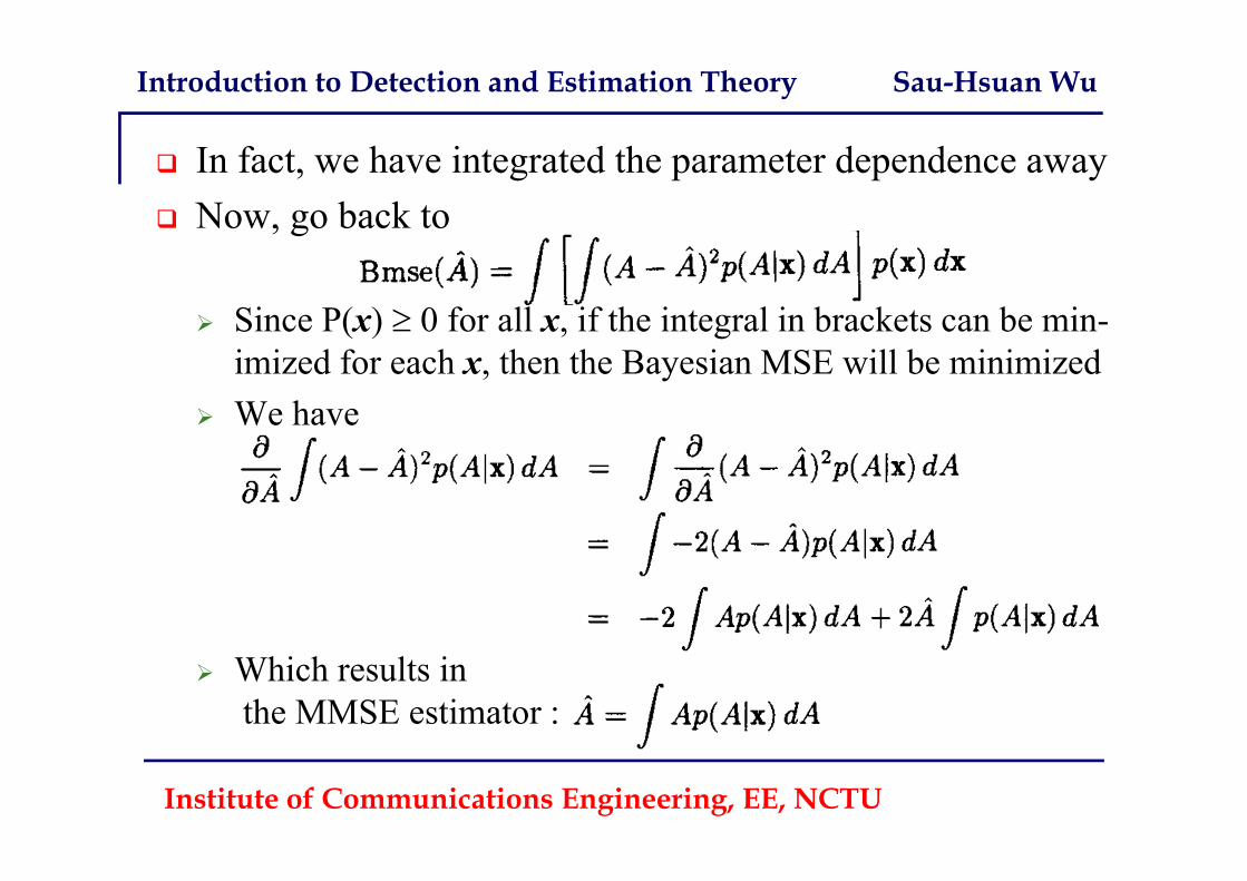
In fact, we have integrated the parameter dependence away Now, go back to
Since P(x) 0 for all x, if the integral in brackets can be min-imized for each x, then the Bayesian MSE will be minimized
We have
Which results inthe MMSE estimator :
Introduction to Detection and Estimation Theory Sau-Hsuan Wu
Institute of Communications Engineering, EE, NCTU
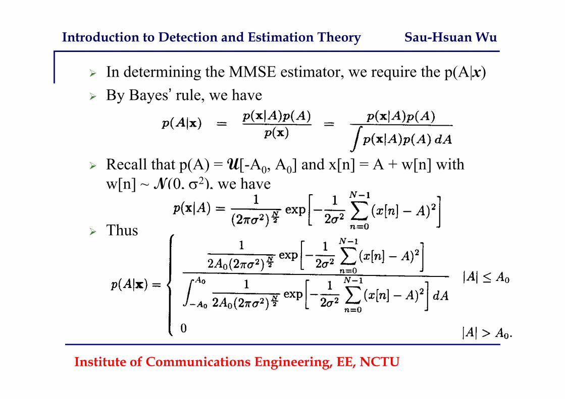
In determining the MMSE estimator, we require the p(A|x) By Bayes’ rule, we have
Recall that p(A) = U[-A0, A0] and x[n] = A + w[n] with w[n] ~ N(0, 2), we have
Thus
Introduction to Detection and Estimation Theory Sau-Hsuan Wu
Institute of Communications Engineering, EE, NCTU
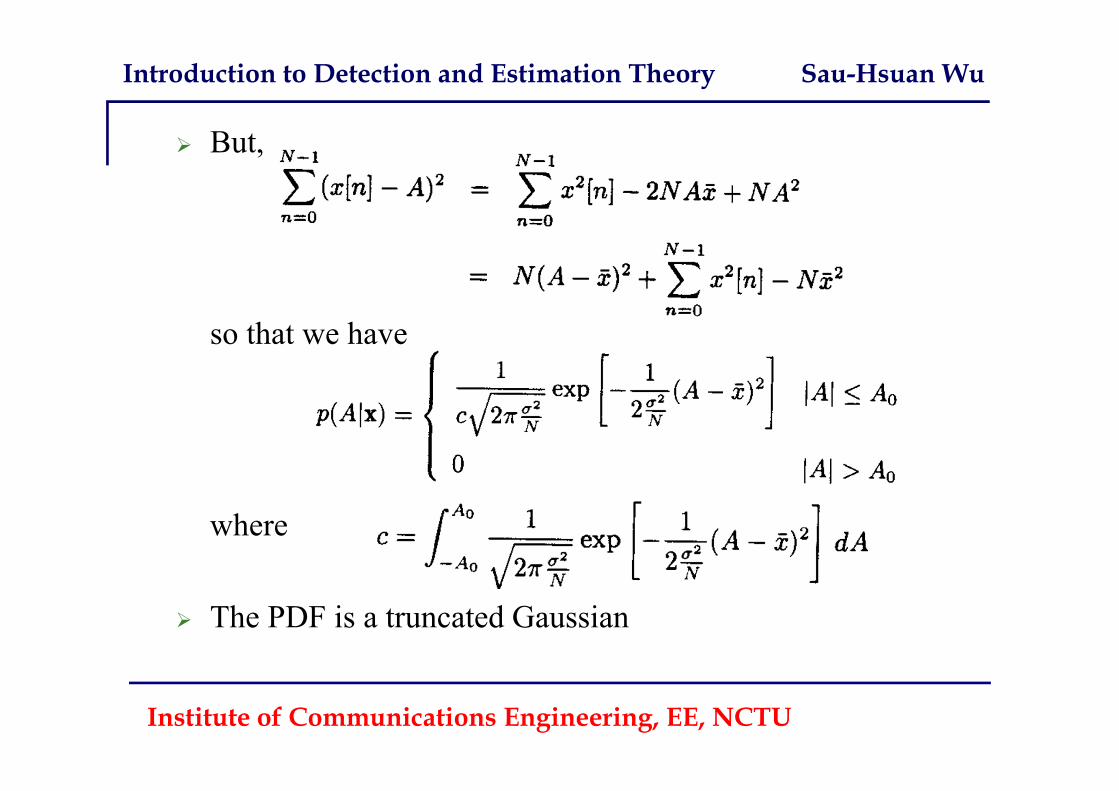
But,
so that we have
where
The PDF is a truncated Gaussian
Introduction to Detection and Estimation Theory Sau-Hsuan Wu
Institute of Communications Engineering, EE, NCTU
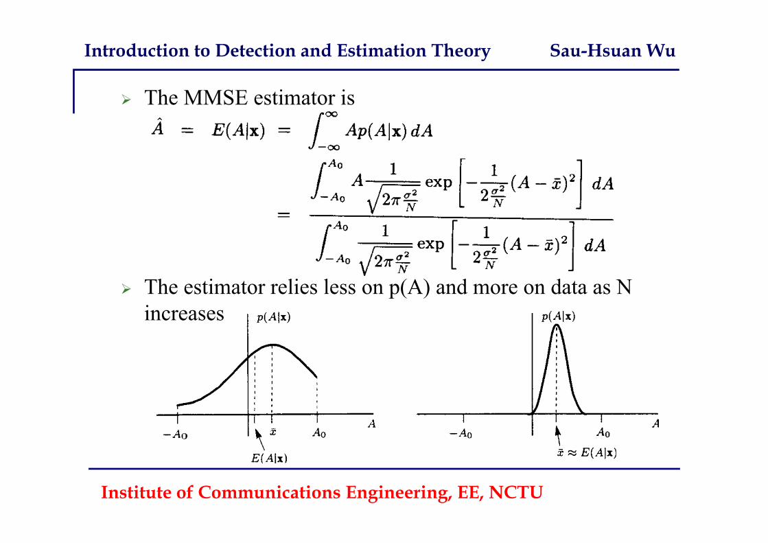
The MMSE estimator is
The estimator relies less on p(A) and more on data as N increases
Introduction to Detection and Estimation Theory Sau-Hsuan Wu
Institute of Communications Engineering, EE, NCTU
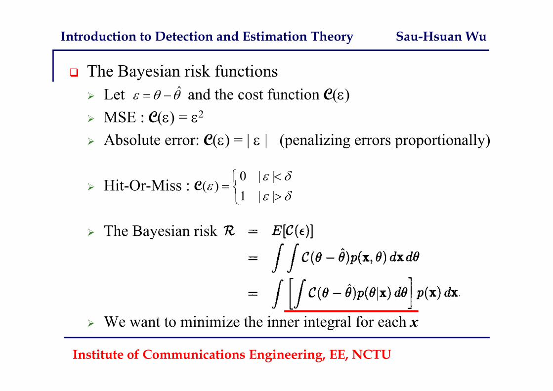
The Bayesian risk functions Let and the cost function C() MSE : C() = 2
Absolute error: C() = | | (penalizing errors proportionally)
Hit-Or-Miss :
The Bayesian risk
We want to minimize the inner integral for each x
ˆ
0 | |( )
1 | |
C
Introduction to Detection and Estimation Theory Sau-Hsuan Wu
Institute of Communications Engineering, EE, NCTU
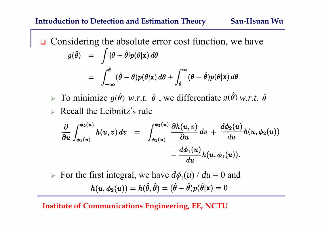
Considering the absolute error cost function, we have
To minimize w.r.t. , we differentiate w.r.t. Recall the Leibnitz’s rule
For the first integral, we have d1(u) / du = 0 and
θ̂ˆ( )g θ ˆ( )g θ θ̂
Introduction to Detection and Estimation Theory Sau-Hsuan Wu
Institute of Communications Engineering, EE, NCTU
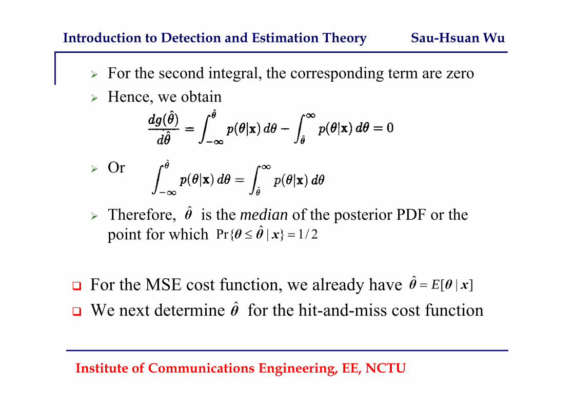
For the second integral, the corresponding term are zero Hence, we obtain
Or
Therefore, is the median of the posterior PDF or the point for which
For the MSE cost function, we already have We next determine for the hit-and-miss cost function
θ̂ˆPr{ | } 1/ 2 θ θ x
ˆ [ | ]Eθ θ x
θ̂
Introduction to Detection and Estimation Theory Sau-Hsuan Wu
Institute of Communications Engineering, EE, NCTU
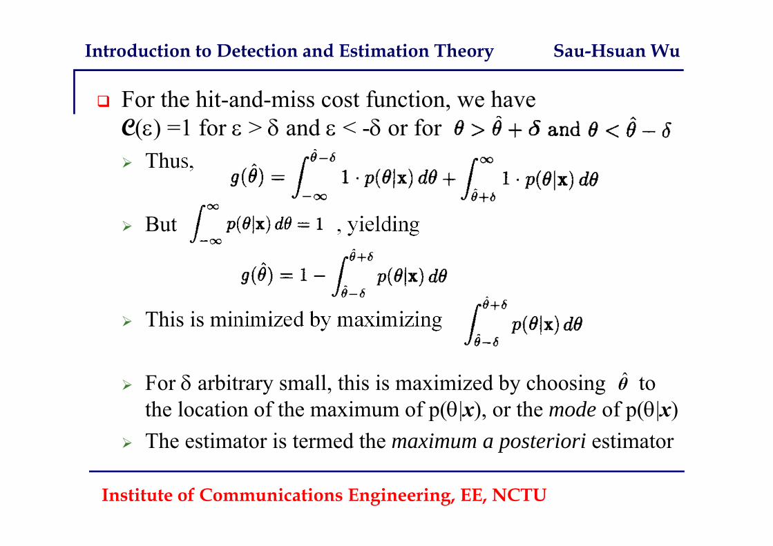
For the hit-and-miss cost function, we have C() =1 for > and < - or for Thus,
But , yielding
This is minimized by maximizing
For arbitrary small, this is maximized by choosing to the location of the maximum of p(|x), or the mode of p(|x)
The estimator is termed the maximum a posteriori estimator
θ̂
Introduction to Detection and Estimation Theory Sau-Hsuan Wu
Institute of Communications Engineering, EE, NCTU
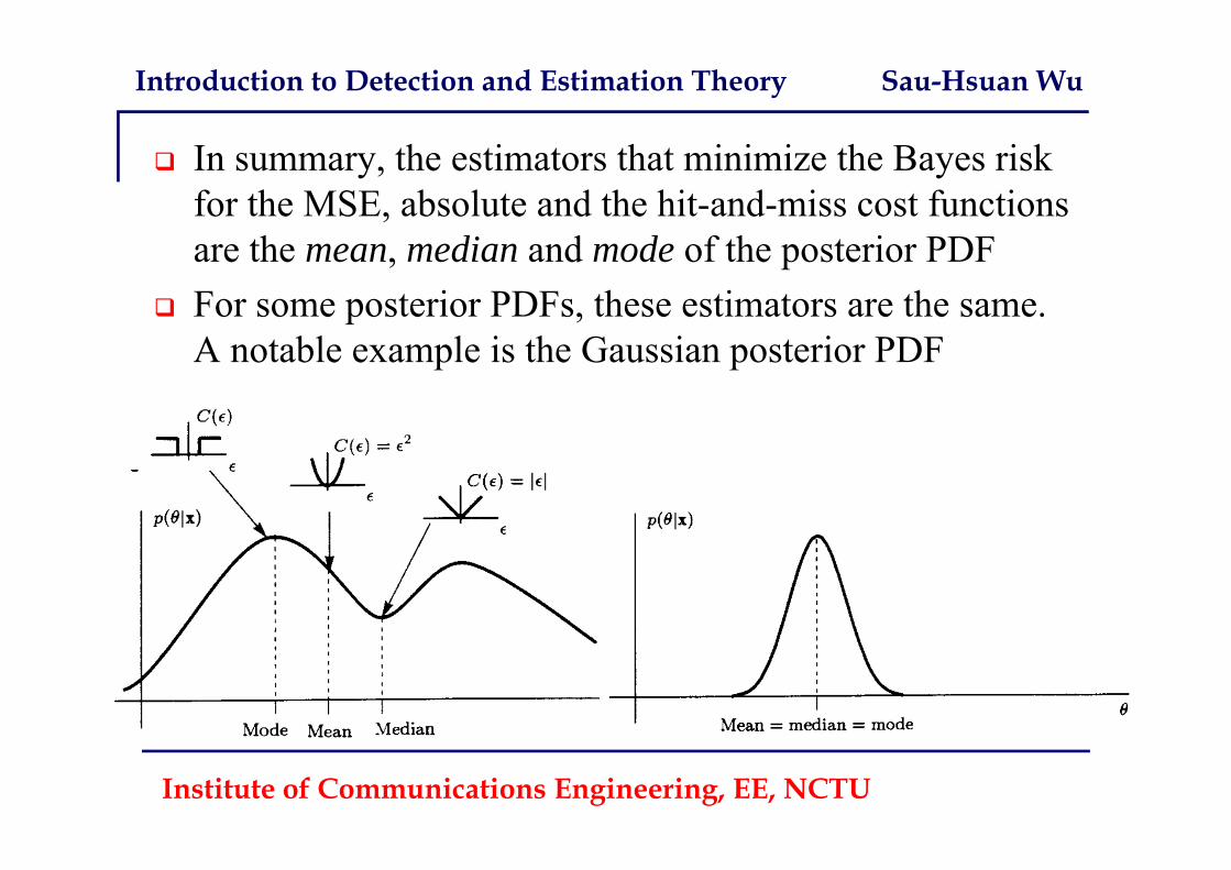
In summary, the estimators that minimize the Bayes risk for the MSE, absolute and the hit-and-miss cost functions are the mean, median and mode of the posterior PDF
For some posterior PDFs, these estimators are the same. A notable example is the Gaussian posterior PDF
Introduction to Detection and Estimation Theory Sau-Hsuan Wu
Institute of Communications Engineering, EE, NCTU 68
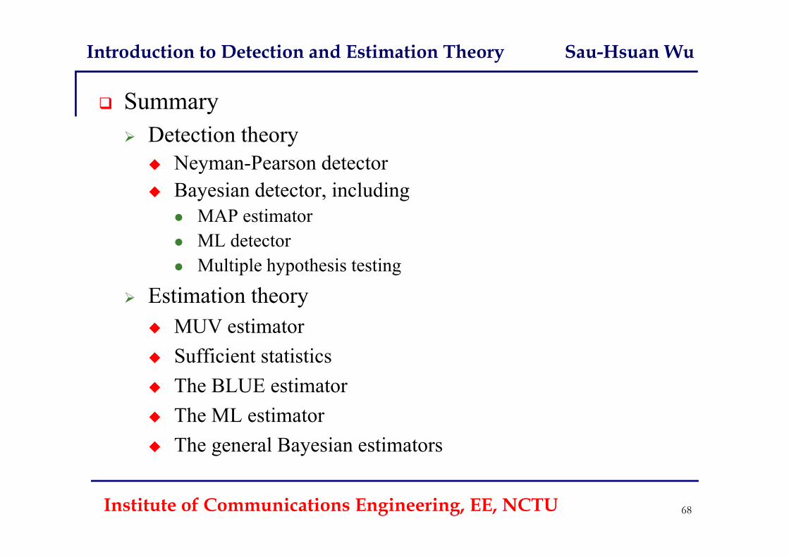
Summary Detection theory
Neyman-Pearson detector Bayesian detector, including
MAP estimator ML detector Multiple hypothesis testing
Estimation theory MUV estimator Sufficient statistics The BLUE estimator The ML estimator The general Bayesian estimators