Detection and Analysis of Anisotropic Scattering in SAR...

Detection and Analysis of Anisotropic Scattering inSAR Data$

ANDREW J. KIM [email protected]

Stochastic Systems Group, Massachusetts Institute of Technology, Cambridge, MA 02139

JOHN W. FISHER III


ALAN S. WILLSKY1


Received December 1, 2000; Revised September 9, 2001; Accepted September 26, 2001

Abstract. Scattering from man-made objects in SAR imagery exhibits aspect and frequency dependencies which

are not well modeled by standard SAR imaging techniques. If ignored, these deviations will reduce recognition

performance due to the model mismatch, but when appropriately accounted for, these deviations from the ideal

point scattering model can be exploited as attributes to better distinguish scatterers and their respective targets.

With this premise in mind, we have developed an efficient modeling framework that incorporates scatterer

anisotropy. One of the products of our analysis is the assignment of an anisotropy label to each scatterer

conveying the degree of anisotropy. Anisotropic behavior is commonly predicted for geometric scatterers

(scatterers with a simple geometric structure), but it may also arise from volumetric scatterers (random

arrangements of interfering point scatterers). Analysis of anisotropy arising from these two modalities shows a

clear source-dependent relationship between the anisotropy classification and parameters of the scatterer. In

particular, the degree of anisotropy is closely related to the size of the scatterer, and increasing the aperture size

reduces the incidence of volumetric anisotropy but preserves the detection rate for geometric anisotropy. This

result helps to address the question in the SAR community regarding the utility of wide-aperture SAR data for

ATR since wide-aperture data reveals geometric anisotropy while resolving volumetric anisotropy into individual

isotropic scatterers.

Key Words: SAR, anisotropy, wide-aperture, multi-resolution, canonical scattering, volumetric scattering, ATR

1. Introduction

Scatterers composing a target in synthetic aperture radar (SAR) imagery often exhibit

nonideal scattering behavior in the form of aspect and frequency dependence, particularly

in wide-aperture or wide-band data. Standard SAR image formation ignores this model

deviation resulting in suboptimal use of the data. The modeling error may furthermore

Multidimensional Systems and Signal Processing, 14, 49–82, 2003# 2003 Kluwer Academic Publishers. Manufactured in The Netherlands.

B This work is sponsored by Air Force Office of Scientific Research grant F49620-96-1-0028 (subcontract BU

GC123919NGD), Office of Naval Research grant N00014-00-1-0089, and DARPA under Wright Patterson grant

F33615-97-1014.

introduce artifacts, such as peak scatterer instability, which unnecessarily complicate the

recognition problem. These deviations from the ideal point scattering model should not be

viewed as a nuisance and approximated away, but they should instead be seen as a useful

attribute which can be used to distinguish scatterers and thus their respective targets. In

this paper, we present a multi-scale analysis for detecting and classifying scatterer

anisotropy in SAR data. This analysis is used for (i) studying the dependence of

the proposed anisotropy attribution on scatterer phenomenology and (ii) assessing the

utility of wide-aperture data in the attribution process and hence for automatic target

recognition (ATR).

There are numerous benefits to knowing the anisotropy of a scatterer which the standard

image formation process ignores. From an imaging standpoint, a better scattering model

allows for more accurate reflectivity estimates since the weighting in the coherent

averaging can be adjusted according to the azimuthal scattering pattern (e.g. with a

matched filter) such as in the work done by Allen et al. [1] and by Chaney et al. [2].

Knowledge of anisotropy may also be used to better suppress interfering scatterers in a

super-resolution image formation algorithm such as Capon’s method [3] or the high

definition imaging proposed by Benitz et al. [4], [5]. In addition to improving reflectivity

estimation, knowledge of a scatterer’s anisotropy is useful as a feature in and of itself.

For a canonical scatterer, one can infer properties about its geometric shape and size

from the observed anisotropy. For instance, a flat plate produces a strong specular

response where the degree of specularity is directly related to the size of the plate in

cross-range. A sphere however produces an isotropic response regardless of the size of

the sphere. Knowledge of the geometry of the individual scatterers on an object may then

be considered as a group to aid the classification of the target under investigation as

described in [9], [10], [11]. Anisotropy information may also be of use in characterizing

the stability of a scatterer. In particular, one would expect the specular response from an

anisotropic canonical scatterer to appear only over a small range in azimuth leading to an

observability that is highly sensitive to azimuthal orientation. Knowledge of the aniso-

tropy however allows such sensitivity to be incorporated into algorithms, such as peak

matching, which would improve ATR performance.

The focus of this paper is to present a method for classifying anisotropy and to study

behavior of the attribution under different conditions. The analysis presented here is

based on a general characterization of azimuthal anisotropy which is not tuned to a

particular canonical scatterer. The basis of our analysis is the sub-aperture pyramid which

is a set of sub-apertures arranged in a pyramidal fashion. The collection of sub-apertures

provides a multi-resolution representation of SAR data. These multiple apertures allow

for the observation of varying degrees of azimuthal anisotropy which are unobservable

under standard SAR image formation. With this pyramidal representation of the data, we

propose a hypothesis test for anisotropy which measures the concentration of scattering

energy across the aperture.

Analysis of this characterization reveals aspects of the phenomenology associated

with anisotropy and how the attribution can be utilized in ATR. In studying the

behavior of our anisotropy characterization, we consider two well known sources of

anisotropy: geometric and volumetric scatterers. Scattering models such as physical

A. J. KIM, J. W. FISHER III AND A. S. WILLSKY50

optics and the Geometric Theory of Diffraction (GTD) give functional forms for radar

scattering from canonical scatterers which clearly convey an azimuthal dependence on

the shape, size, and orientation of a scatterer. These models are based on very specific

assumptions about the configuration of scatterer, such as equal-sized plates in a dihedral

or pairwise orthogonality of plates in a trihedral. As our analysis is concerned with

producing a general characterization of anisotropy, we will not entangle ourselves with

such fine structural details. This approach allows us to consider the broader class of

what we call geometric scatterers which include not only canonical scatterers but also

scatterers that deviate from canonicity. Besides geometric scatterers, anisotropy may

also arise from a volumetric scatterer which is a collection of closely located point

scatterers that interfere with each other. The anisotropy exhibited by volumetric

scatterers, however, is not as stable as the anisotropy produced by geometric scatterers.

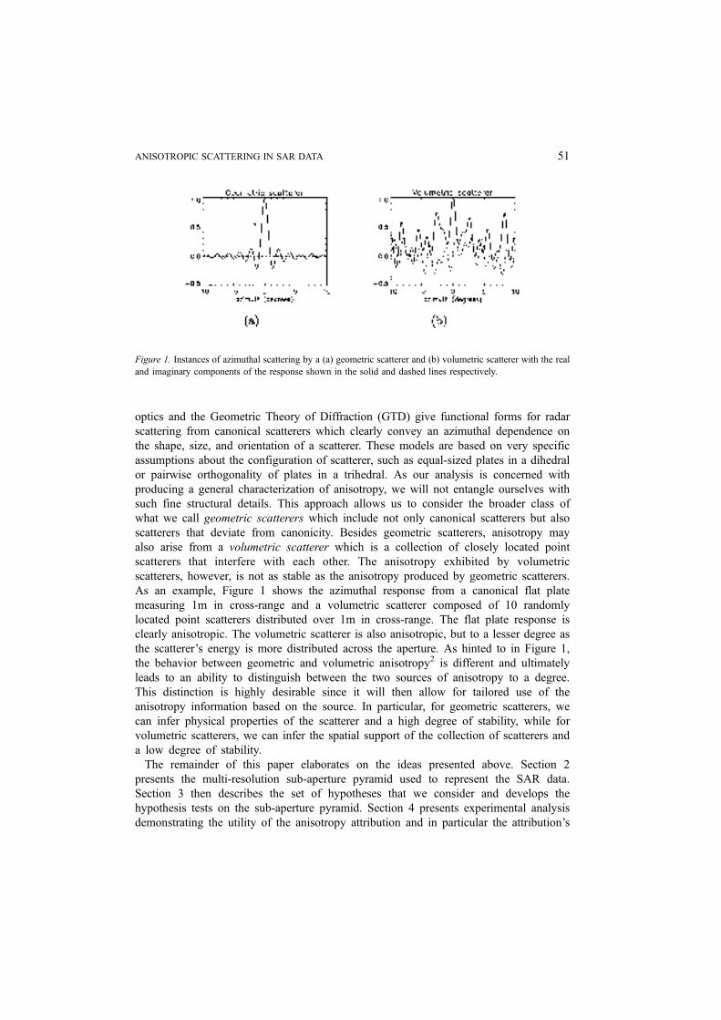
As an example, Figure 1 shows the azimuthal response from a canonical flat plate

measuring 1m in cross-range and a volumetric scatterer composed of 10 randomly

located point scatterers distributed over 1m in cross-range. The flat plate response is

clearly anisotropic. The volumetric scatterer is also anisotropic, but to a lesser degree as

the scatterer’s energy is more distributed across the aperture. As hinted to in Figure 1,

the behavior between geometric and volumetric anisotropy2 is different and ultimately

leads to an ability to distinguish between the two sources of anisotropy to a degree.

This distinction is highly desirable since it will then allow for tailored use of the

anisotropy information based on the source. In particular, for geometric scatterers, we

can infer physical properties of the scatterer and a high degree of stability, while for

volumetric scatterers, we can infer the spatial support of the collection of scatterers and

a low degree of stability.

The remainder of this paper elaborates on the ideas presented above. Section 2

presents the multi-resolution sub-aperture pyramid used to represent the SAR data.

Section 3 then describes the set of hypotheses that we consider and develops the

hypothesis tests on the sub-aperture pyramid. Section 4 presents experimental analysis

demonstrating the utility of the anisotropy attribution and in particular the attribution’s

Figure 1. Instances of azimuthal scattering by a (a) geometric scatterer and (b) volumetric scatterer with the real

and imaginary components of the response shown in the solid and dashed lines respectively.

ANISOTROPIC SCATTERING IN SAR DATA 51

relation to the scatterer phenomenology. The paper concludes with a summary and

discussion in Section 5.

2. Sub-Aperture Analysis

The foundation of our analysis is the sub-aperture pyramid which we present in this

section. This structure is motivated by the scattering physics involved in SAR and

presents the data in a way that allows for simple and intuitively reasonable hypothesis

tests. Because of the linear structure of the aperture, we associate it with an interval of the

real line throughout this paper. In particular, the full-aperture is denoted by the interval

[0, 1) ¼ {t |0 � t < 1}.

2.1. Definition

The intuitive idea of the sub-aperture pyramid is to generate an over-complete covering of

the full-aperture with sub-apertures that can be arranged in a pyramidal structure. These

sub-apertures will be used both to form our reflectivity estimates and to represent our set of

candidate anisotropy hypotheses. The prototypical sub-aperture covering that we use

throughout this paper is the half-overlapping, half-aperture pyramid shown in Figure 2.

Formally, we take a sub-aperture pyramid to be a set S of sub-apertures with the

following structure. The set S is partitioned into smaller sets Sm all the elements of which

have a particular sub-aperture length as illustrated in Figure 2. S0 refers to the set

consisting of the largest sub-apertures, and SM refers to the set of the smallest sub-

apertures. A second subscript on S denotes a specific sub-aperture at the given scale. Note

that any sub-aperture can be used to form a SAR image. The images formed with a smaller

value of m, i.e. with a larger aperture, have a finer cross-range imaging resolution because

of the inverse relationship between resolution cell size and aperture length. This point is

illustrated in Figure 2 where if the full-aperture produces a resolution cell of size �, thenthe half and quarter-apertures produce resolution cells of sizes 2� and 4�, respectively.Note that this inverse relationship between sub-aperture size and resolution cell size

Figure 2. Illustration of the three level, half-overlapping, half-aperture pyramid. Left: Sub-apertures composing

the pyramid. Right: Resolution cell size associated with reflectivity estimates formed from sub-apertures at the


may lead to ambiguity when terms such as ‘‘coarse’’ and ‘‘fine’’ are used. For instance,

a ‘‘coarser’’ (i.e. larger) sub-aperture produces a ‘‘finer’’ resolution cell. To avoid any

ambiguity, we will explicitly use the terms ‘‘smaller’’ and ‘‘larger’’ when referring to sub-

aperture sizes and the terms ‘‘finer’’ and ‘‘coarser’’ when referring to resolution cell sizes.

The idea of the sub-aperture pyramid is to present SAR data in an over-complete

representation at a variety of cross-range resolution versus azimuthal3 resolution trade-

offs. Recall that cross-range resolution is inversely proportional to aperture length. Thus, at

lower levels of the sub-aperture pyramid, spatial resolution has been exchanged for

azimuthal resolution, i.e. the ability to better observe anisotropic phenomena. This is

the classic time–frequency resolution tradeoff in Fourier analysis, and each level of the

pyramid represents the data under a particular cross-range–azimuth resolution. The

presence of multiple resolutions is attractive because we expect the best representation

to depend on the underlying anisotropy. In particular, it is the set which has the sub-

aperture which best captures the scattering energy with minimal aperture length, i.e. the

closest resemblance to a matched-filter using an indicator function over a sub-aperture.

Since the scatterer anisotropy (and thus best sub-aperture representation) cannot be known

apriori, an over-complete basis, such as that provided by the sub-aperture pyramid, is

useful in finding the best representation.

Having conveyed the intuition behind the sub-aperture pyramid, we now establish the

necessary conditions on the pyramid for what follows later. In particular, the following

conditions are imposed on S:

(A) 8Sm,i, Sm,i � [0, 1),

(B) 8Sm,i, 9 a partition P(m, i) � SM of Sm,i, and

(C) 8Sm,i with m � 1, 9Sm�1, j such that Sm,i � Sm�1, j.

The first condition simply restricts the sub-apertures to be a subset of the available

aperture. Motivated by our search for concentrated unimodal scattering in azimuth, we

only consider the special case where each sub-aperture is a connected interval. Moreover,

we also assume that S0,0 is the full-aperture to allow for consideration of the minimal

degree of anisotropy and allow for the finest imaging resolution permissible. The second

condition insures that each sub-aperture can be represented by a partition of smallest-sized

sub-apertures. This condition will allow for the set of measurements obtained from SM to

form a sufficient statistic for all the measurements in S. Thus, although other sub-aperture

measurements will be referred to in this paper for intuition and interpretation, all

computation can be done using only measurements from the smallest sub-apertures. The

third condition asserts that each sub-aperture, except those in S0, has a parent sub-aperture

which contains it. This last condition is not a fundamentally necessity for our anisotropy

analysis, however, we use this condition because it permits us to construct an intuitive

telescopic hypothesis test on a tree which will not only afford computational efficiency

but also robustness. Herein, the term sub-aperture pyramid refers to one satisfying

conditions (A)–(C).

Now, focusing our attention on a particular location in the scene, each sub-aperture Sm,ican be used to generate an associated reflectivity measurement qm,i. The collection of


reflectivity measurements from the different offset sub-apertures in SM are formed into a

vector which is denoted by qM. The measured sub-aperture reflectivity qm,i is obtained in

the same fashion as in standard SAR image formation, i.e.

qm;i ¼ZSm;i

aðtÞdt ð1Þ

where a(t) is the azimuthal response of the scatterer4. Although reflectivity measurements

from smaller sub-apertures have an associated coarser resolution, they are less susceptible

to azimuthal variations and provide a means for measuring scattering energy across the

aperture. Note that the measured reflectivity is not normalized with respect to the sub-

aperture length5. Thus, when interested in the actual reflectivity estimate, one should

divide the measured sub-aperture reflectivity qm,i by the sub-aperture length Lm,i ¼ �(Sm,i),where � denotes Lebesgue measure.

2.2. Interpretation and Motivation

Different types and sizes of geometric scatterers exhibit different aspect dependencies. The

motivation for using the sub-aperture pyramid is that the pyramid is expected to reveal

distinguishing aspect dependences in the scattering. For example, a metal sphere has a

strong response in all directions and thus produces a strong consistent reflectivity estimate

from each of the sub-apertures. However, as depicted in Figure 3, a flat plate produces a

specular response which is significantly stronger when oriented broadside with respect to

the radar. Thus, the reflectivity estimates vary across the sub-apertures with the largest

estimate coming from the sub-aperture oriented broadside to the plate. Furthermore,

because various sized sub-apertures are used, the duration of the broadside flash is also

Figure 3. The response of a 1m � 1m flat plate and a depiction of the reflectivity estimate for each of the sub-

apertures. Darker shaded sub-apertures convey larger reflectivity estimates.


captured in this representation. To see this point, note that for all sub-apertures which

reside within the main-lobe of the response, the reflectivity estimates are consistently

large. As the sub-aperture is expanded, however, the additional signal energy received is

relatively insignificant thereby lowering the reflectivity estimate which is normalized with

respect to sub-aperture length. Not only does using an excessively large sub-aperture lower

the normalized reflectivity estimate, but it also results in a noisier estimate because the

additional portion of the aperture being incorporated is dominated by noise6. To illustrate

that this anisotropic phenomena is clearly present in real data, we show in Figure 4 a three

level, disjoint, half-aperture pyramid and the corresponding sub-aperture images for a

BMP-2 from the MSTAR public release dataset [6] which uses a 2.8j aperture. Even in

this narrow aperture setting, we clearly see that the response associated with the middle

section of the aperture contains the majority of the energy from the large scatterer at the

front of the vehicle.

3. Anisotropic Scattering Models

Having presented the sub-aperture pyramid, we now proceed to formulate our hypothesis

testing problem for anisotropy where the hypotheses are formulated over the sub-aperture

pyramid. Our goal is to use the sub-aperture pyramid to develop a general characterization

of anisotropy that is not overly-sensitive to azimuthal dependencies such as those

produced by geometric scatterers with non-canonical deviations. In particular, we only

intend to measure the concentration of unimodal azimuthal scattering and are not

concerned with the minor deviations in the azimuthal response that occur with slight

changes in scatterer geometry. Two models are presented here that yield this character-

ization. The first is a simple isolated scatterer model with an intuitive sufficient statistic.

This test, however, is susceptible to the interference from neighboring scatterers. This

shortcoming motivates the second model which explicitly accounts for the effects of

Figure 4. Left: Disjoint half-aperture pyramid. Right: Corresponding sub-aperture images of a BMP-2 at a 17jelevation and 0j azimuth. For each image, the front of the vehicle is the portion nearest the left edge of the image.


neighboring scatterers. The tests presented in this section are for a fixed scattering location

which we assume to be specified. These locations could come from a peak extraction

process (for peak attribution as is done in Section 4) or a pre-specified grid (for an image

of anisotropy).

3.1. Isolated Scatterer Model

For each sub-aperture Sm,i, we define an associated scattering hypothesis Hm,i over the

aperture t via

Hm;i : aðtÞ ¼ A1Sm;iðtÞ ð2Þ

where 1Sm;ið�Þ denotes the indicator function over Sm,i and A is the unknown scattering

amplitude of the signal. Thus, each hypothesis corresponds to a scattering response that is

uniform over the sub-aperture in question and zero elsewhere. Clearly, this model is an

idealization of anisotropic scattering, but because we are only interested in obtaining a

general characterization of anisotropy, this model serves our purposes. The set of all

possible hypotheses associated with the sub-aperture pyramid is denoted as H.

A reasonable choice of features to test these hypotheses would be all the measured sub-

aperture reflectivities {qm,i}. From the definition of the qm,i in Eq. (1) and partition

property (B), it is sufficient to consider the vector qM of measurements from the smallest

sub-apertures since any sub-aperture reflectivity qm,i can be computed from qM by

summing all the qM,j for which the associated SM,j form a partition of Sm,i, i.e.

qm;i ¼X

jjSM ; j2Pðm;iÞqM ; j:

As an example, for the three level, half-overlapping, half-aperture pyramid in Figure 2,

q1,1 ¼ q2,2 þ q2,4 since S2,2 and S2,4 form a disjoint union of S1,1, i.e. S1,1 ¼ S2,2 [ S2,4 and

S2,2 \ S2,4 ¼ t. Because qM is a sufficient statistic for our sub-aperture reflectivities,

we take it as our feature vector. The value of this feature vector under hypothesis Hm,i and

A ¼ 1 is denoted as b(m, i) whose jth element is given by

bðm; iÞj ¼ZSM ; j

1Sm;iðtÞdt

¼ �ðSM ; j \ Sm;iÞ; ð3Þ

i.e. b(m, i)j is the portion of the response 1Sm;iðtÞ one expects to see over the jth sub-apertureat scale M. We now define our scattering model conditioned on anisotropy hypothesis Hm,i

as the signal plus noise model

qM ; j ¼ZSM ; j

A1Sm; i ðtÞ þ �ðtÞ dt; ð4Þ


where �(t) is circularly complex white Gaussian noise with spectral density 2�2. Thischaracterization leads to the model

Hm;i : qM ¼ Abðm; iÞ þ e; with e � Nð0; 2�2LÞ; ð5Þ

where L is the noise covariance structure inherited from the sub-aperture pyramid. The

noise in the measured reflectivities in Eq. (5) are characterized as zero-mean circularly

complex Gaussians with covariances dictated by the amount of sub-aperture overlap. The

elements of the covariance matrix L are thus given by [L]i,j ¼ �(SM,i \ SM,j), which for the

half-overlapping half-aperture pyramid in Figure 2 is

L ¼ 1

2M

1 :5 0

:5 O O

O O :5

0 :5 1

2666666664

3777777775:

To classify the anisotropy of a scatterer from our vector of sub-aperture measurements

qM, we apply a log-likelihood ratio test to the model in Eq. (5) where each log-likelihood is

compared to the full-aperture hypothesis H0,0. Because there is the unknown reflectivity

parameter A, we use a generalized log-likelihood ratio (GLLR) test where for each

hypothesis, we take A to be the maximum likelihood (ML) estimate under that hypothesis.

For Hm,i, the matched-filter gives the ML estimate as ^A ¼ qm;i=Lm;i . Using this estimate

results in the GLLR

‘m;i ¼1

4�2

1

Lm;ijqm;ij2 � jq0;0j2

: ð6Þ

Thus, the most likely sub-aperture in this case is the one whose average energy is largest.

We note the similarity here to the approach taken by Chaney et al. [2] in which they

replace, within the image, the standard full-aperture reflectivity estimate with the

maximum sub-aperture reflectivity estimate jqm;i=Lm;ij, thus using normalized reflectivity

(instead of normalized energy) as their criterion for choosing anisotropy. Their approach

however is based on intuitive arguments and not a derived statistic. Although this

difference may be seemingly small, the effect is quite significant. In particular, using

normalized reflectivity, instead of energy, over-compensates for decreasing aperture size.

This over-compensation biases their test to choose smaller sub-aperture hypotheses and

thus produces images with an excessively coarse imaging resolution. Furthermore, their

technique does not address the very significant effect of neighboring scatterers that we

discuss next. Thus, when used for image formation, our technique better preserves the fine


resolution of the imagery, where appropriate, since the technique produces more accurate

anisotropy classifications.

Though simple and intuitive, the GLLR in Eq. (6) is susceptible to the effects of close

proximity neighboring scatterers which are not accounted for in our model in Eq. (4).

Recall that the images formed by the smaller sub-apertures have a coarser imaging

resolution, and thus the hypotheses are not all consistent in terms of the resolution cell

contents. In particular, if a scatterer were located outside the finest resolution cell but

within a coarser resolution cell, then the finest resolution reflectivity q0,0 would be 0,

but qm,i would be large if the resolution cell associated with scale m included the scatterer.

We illustrate this point with the example shown in Figure 5. Here a scatterer with

amplitude A is located outside the finest resolution cell of size � but is contained within

the coarser resolution cell of size 2� associated with half-aperture estimates. If this

scatterer is isotropic, then the response is the complex exponential illustrated. Integrating

over the full aperture gives a 0 reflectivity estimate as expected, but integrating over a half

aperture produces a reflectivity with magnitude A=ffiffiffi2

p. Eq. (6) would then classify the

center of the resolution cell as anisotropic, even though no scatterer is present in the finest

resolution cell.

The problem above is a consequence of not modeling the influence of neighboring

scatterers. One of the ways in which the neighboring scatterer manifests itself is through

the corruption of the estimated reflectivity as the size of the resolution cell varies. Instead

of choosing the ML estimate ^A ¼ qm;i=Lm;i as the unknown reflectivity, we can choose

the best reflectivity estimate constrained to lie in the finest resolution cell associated with

the full-aperture estimate q0,0. Choosing ^A ¼ q0;0=Lm;i (where the normalization by Lm,iaccounts for the fact that the modeled azimuthal response is concentrated in a sub-

aperture) for all hypotheses can be shown to produce the GLLR statistic

‘m;i ¼1

4�2

1

Lm;ijqm;ij2 �

1

Lm;ijq0;0 � qm;ij2 �

1

L0;0jq0;0j2

: ð7Þ

This statistic is identical to that in Eq. (6) except for the extra term comparing the

reflectivity estimates q0,0 and qm,i. Recall that Eq. (6) compared the average energy in a

Figure 5. Illustration of how a scatterer that is not in the finest resolution cell can produce a false anisotropy

classification from Eq. (6).


sub-aperture to the full-aperture. This new GLLR accounts for the average energy outside

the hypothesized sub-aperture as well. Viewed differently, under hypothesis Hm,i and our

scattering model in Eq. (4)–(5), the values of q0,0 and qm,i should simply be noisy

perturbations of each other. The new term penalizes when this is not the case thereby

enforcing a consistency of the resolution cell contents. Under the example in Figure 5,

since the the contribution of each of the half-apertures would be the same, the GLLR is

equal to zero for all hypotheses, which is reasonable, since there is no underlying

scattering at the focused location.

3.2. Multiple Scatterer Model

The modification in Eq. (7) addresses the problem when a neighboring scatterer is

isotropic, however, when the neighboring scatterer is anisotropic, problems such as that

illustrated by the example in Figure 5 can still arise as the contribution from the interfering

scatterer will not integrate out over the full-aperture estimate. To account for this

phenomenon, we generalize the model in Eq. (4) to explicitly include multiple scatterers.

In particular, we consider the possibility of regularly spaced neighboring scatterers (each

with its own anisotropy hypothesis) and incorporate their effects into the anisotropy test.

Doing so, we obtain the GLL statistic7

‘ ¼ 1

2�2qMV L�1 � 2L�1BP þ PVBVL�1BP

� qM ð8Þ

where B and P are defined in Eqs. (14) and (15) of Appendix A. We note that the

hypothesis enters into Eq. (8) only via B and P, and thus, the weighting matrix in the

brackets is data independent and can be precomputed allowing for a computationally

simple GLL that corresponds to a norm on qM.

3.3. Telescopic Testing

The sub-aperture pyramid which we use to form our measurements and base our

hypotheses is convenient not only for providing anisotropy information, but also for

providing an efficient means of performing the hypothesis tests. We can obtain an efficient

Figure 6. Illustration of how the anisotropy testing can be done in a decision-directed fashion by starting with the

largest aperture and at each scale, inspecting only the children of the most likely sub-aperture. Darker shading of

the sub-apertures indicate higher likelihoods. Dashed lines denote which hypotheses are tested, and solid lines

denote the branch traversed.


approximation to the test by evaluating only a small subset of the candidate hypotheses.

Due to the nested structure of the sub-apertures (condition (C) in Section 2), we can

perform the tests in a telescopic fashion by traversing down a branch in the tree of sub-

apertures as depicted in Figure 6. On the pyramid, we expect the likelihoods to increase as

the hypothesized sub-apertures ‘‘shrink down to’’ the correct sub-aperture, and then to

decrease as the hypothesized sub-apertures ‘‘shrink beyond’’ the correct sub-aperture. This

intuition motivates performing the hypothesis test in the following manner:

Step 1. Start with the set of largest sub-aperture(s) at scale m ¼ 0. Find the most likely

hypothesis at that scale and denote this hypothesis as H0;i0*.

Step 2. Consider those hypotheses at scale m þ 1 for which Smþ1;imþ1� Sm;im*. Find the one

which has the highest likelihood and denote this hypothesis as Hmþ1;i*mþ1.

Step 3. If the parent is more likely (i.e. ‘m;im* > ‘mþ1;i*mþ1), then stop and return Hm;im*

as the

estimated hypothesis.

Step 4. If m þ 1 ¼ M, we are at the bottom of the tree, so stop and return Hmþ1;i*mþ1as the

estimated hypothesis. Otherwise, increment m and goto step 2.

This procedure provides an efficient approximation to finding the ML hypothesis without

evaluating all the likelihoods. If Hm,i is the hypothesis with the highest likelihood, then all

that is required for it to be chosen by this scheme is that:

(D) At each scale n < m, the sub-aperture at scale n with the highest likelihood is an

ancestor of Sm,i.

(E) The sequence of likelihoods increases as the branch is traversed until Sm,i is reached.

Intuitively, these are reasonable conditions that one would usually expect to hold given the

interpretation that our tests measure average energy over a sub-aperture. This intuition can

be justified under the isolated scattering models. In particular, consider the expected value

of ‘n, j when the true hypothesis is Hm,i and the proportion of overlap between Sn, j and Sm,iis given by � ¼ �ðSn; j\Sm;iÞ

�ðSm;iÞ . For Eq. (6), in which the estimate A ¼ qm,j is used, the expected

value of the GLLR is

E ‘n; j j Hm;i

� ¼ E 1

Ln; jjqn; jj2 � jq0;0j2

��Hm;i

¼ �2

Ln; j� 1

� �jAj2 þ ð2Ln; j þ 1Þ�2

c�2

Ln; j� 1

� �jAj2 ð9Þ

where the approximation is for high SNR scattering. From this equation, we see the

intuitive behavior described above. In particular, to maximize the GLLR at each scale

n < m, we would choose a sub-aperture that maximizes � (producing � ¼ 1) and thus

completely overlaps the true sub-aperture, i.e. an ancestor of the true sub-aperture Hm,i.


Furthermore, for all ancestors of Hm,i, the expected value of the GLLR increases with

decreasing sub-aperture length, i.e. the sequence of expected log-likelihoods increases as

the branch is traversed. When the hypothesized sub-aperture becomes too small, the

overlap is � ¼ Ln, j /Lm,i, and the expected GLLR decreases. So, as intuition would

suggest, the expected value of the GLLR (i) is maximized for the true hypothesis and (ii)

obeys conditions (D) and (E) for Eq. (6) under high SNR.

Similarly, for Eq. (7), in which the estimate A ¼ q0,0 /Lm,i is used, the expected value of

the GLLR is

E ‘n; j j Hm;i

� ¼ E 1

Ln; jjqn; jj2 �

1

Ln; jjq0;0 � qn; jj2 � jq0;0j2

�� Hm;i

¼ 2�� 1

Ln; j� 1

� �jAj2 � 1

Ln; j� 1

� �2�2

c2�� 1

Ln; j� 1

� �jAj2 ð10Þ

where the approximation is for high SNR scattering. The behavior with respect to � and

Ln,j follow the same trend as for Eq. (9) and thus again supports our intuition for using the

telescopic testing. Because of the difficult form of our regularized multiple scatterer log-

likelihood given in Eq. (16), we have not shown that the same pattern holds for this

extended test, however, intuition and the success demonstrated in the empirical results of

Section 4 lead us to believe this behavior holds here as well.

Besides computational efficiency, performing the hypothesis tests in a telescopic fashion

also enforces a form of consistency in the sub-apertures tested. In particular, in order for a

specific sub-aperture to be chosen, its ancestor hypotheses have to be chosen in the testing

at the previous scales. Enforcing such a progression of likelihoods protects against

anomalies where a small sub-aperture could possess a high GLLR while none of its

ancestors do, such as in the example associated with Figure 5.

3.4. Boxcar Model Deviations

The boxcar hypotheses defined in Eq. (2) are simplified models to which real scatterers do

not exactly correspond. One may question whether deviations from this model may

drastically effect our hypothesis tests. For example, if the scattering has a sinc(�) like

dependence in azimuth, then the sidelobes8 will have a large response for a strong scatter

and may not be well modeled as additive in the measurement noise e. To address this

issue, we incorporate deviations from the boxcar response into our model. In particular, we

start by assuming the underlying normalized scattering pattern has been perturbed by

white Gaussian noise. For the isolated scatterer model, this modification changes the

model response in Eq. (3) to

bðm; iÞj ¼ZSM ; j

1Sm;i ðtÞ þ �ðtÞ dt


where �(t) is a circularly complex white Gaussian process with spectral density 2 2 and is

independent of the measurement noise �(t). Thus, our modeled measurement vector is now

a random vector characterized as

bðm; iÞ � N ðbðm; iÞ; 2 2LÞ:

The resulting measurement model is then

Hm;i : qM ¼ Abðm; iÞ þ w; with w � Nð0; 2ðjAj2 2 þ �2ÞLÞ:

Thus, we have essentially the same model as in Eq. (5) except that the variance of the

noise now depends affinely on the square-magnitude of the underlying scatterer. For

consistency, the full-aperture reflectivity estimate is used as the estimate of A in the overall

noise variance under each hypothesis. Thus, the statistics for all the hypotheses are scaled

by the same factor, and the hypothesis that maximizes the likelihood is not changed by the

incorporation of this boxcar deviation.

4. Experimental Analysis

In this section, we examine the behavior of the anisotropy characterization developed in

the previous section by studying the dependence on anisotropic phenomenology. In

particular, the extended test based on the multiple scatterer model (assuming full-aperture

interfering scatterers) is used within the telescopic testing procedure9. We start our analysis

using narrow-aperture data because of its prevalence in the SAR community. Specifically,

we use the MSTAR public release data [6] and data synthetically generated according to

MSTAR operational parameters, i.e. a 0.32m cross-range resolution (2.8j aperture),

9.6GHz center frequency, and 0.25m range resolution (590MHz bandwidth). We empha-

size that our use of MSTAR parameters is to help promote intuitive understanding, and the

results can always be scaled with respect to the aperture size for other settings. For our

experiments, we use the three level, half-overlapping, half-aperture pyramid10 depicted in

Figure 2. The number of neighboring scatterers considered is set by K ¼ 6 and their

spacing is set by the MSTAR oversampling rate of �r /�p ¼ 1.25. The value of the

regularization parameter on neighboring reflectivities is set by � ¼ 0.5. Deviations from

the boxcar model are accounted for by setting ¼ 0.1.

To first demonstrate that our test reveals anisotropic behavior in real data, we show in

Figure 7 the anisotropy attributions for peaks extracted from a BMP-2 tank at 0j, 30j,60j, and 90j azimuths and a 17j depression. Each image displays the log-magnitude

reflectivities using darker shades to indicate stronger reflectivities. Peak locations and

anisotropy characterizations are given by the symbol overlays in each image. A circle

denotes a full-aperture classification; a square denotes a half-aperture classification; a

triangle denotes a quarter-aperture classification. Even though the aperture associated with


this data set is relatively small at 2.8j, we note that we are still able to detect anisotropic

scattering particularly at cardinal azimuthal orientations.

The images in Figure 7 show that scatterers are being classified as anisotropic; however,

the images do not convey how useful that information is in characterizing targets. This

topic is addressed by Kim, et al. [7] where anisotropy is used as an attribution in a peak-

based Bayes classifier. One of the more interesting results in that work is that scatterer

anisotropy is significantly more stable at near-cardinal target orientations than at off-

Figure 7. Anisotropy characterization of peaks extractions on a BMP-2 tank at (a) 0j, (b) 30j, (c) 60j, and(d) 90j azimuths.


cardinal orientations which argues for at least two distinct sources of anisotropy. In

particular, we expect geometric scattering to dominate the near-cardinal orientations and

produce consistent anisotropy attributions but volumetric scattering to dominate at off-

cardinal orientations and produce erratic anisotropy attributions. To verify this intuition,

we separately study our proposed anisotropy characterization for the canonical flat plate

and volumetric scatterers using synthesized data. In both cases, we use what we call an

anisotropy plot to convey the dependence of our anisotropy classification on an underlying

parameter. In the case of the canonical flat plate, this parameter is the plate size, and in the

case of the volumetric scatterer, this parameter is the distribution of constituent scatterers.

4.1. Geometric Anisotropy

To examine geometric anisotropy, we synthesize azimuthal data for the flat plate according

to the physical optics model using MSTAR parameters. To generate the associated

anisotropy plots, we use probability estimates based on Monte Carlo runs involving

8192 trials for each plate size where the scatterer is taken at broadside and white Gaussian

noise is added across the aperture. The PSNR of the signal is kept constant at PSNR ¼20dB, thus noise variance scales with the maximum peak reflectivity.

The anisotropy plot under these settings is shown in Figure 8(a). Contained in this figure

are three curves each of which represents the probability of a particular anisotropy

classification conditioned on the size of the scatterer. Thus, the three values for a given

plate size represent the PMF of these anisotropy classifications (i.e. full, half, and quarter-

aperture) conditioned on that plate size. As expected, the full-aperture classification

dominates for the smaller plate sizes. As plate size is increased, the half-aperture

classification starts to dominate. Between 0.8m and 1m, the half-aperture classification

probability is approximately one. The noiseless azimuthal response for a plate size in the

middle of this region (0.9m) is shown in Figure 9(a) which is quite reasonably classified as

half-aperture. The solid curve in the figure represents the real component of the response,

and the dashed curve represents the imaginary component. The vertical lines are a visual

aid dividing the aperture into eighths. As plate size is increased beyond 1m, the

classification transitions from half-aperture to quarter-aperture in the anisotropy plot of

Figure 8. Anisotropy plots for a square plate in Gaussian noise at 20dB PSNR. (a) no azimuthal and location

uncertainty; (b) maximal azimuthal uncertainty and no location uncertainty; (c) maximal azimuthal uncertainty

and location uncertainty given by peak extraction.


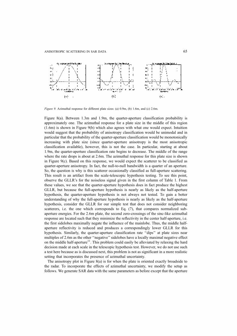
Figure 8(a). Between 1.3m and 1.9m, the quarter-aperture classification probability is

approximately one. The azimuthal response for a plate size in the middle of this region

(1.6m) is shown in Figure 9(b) which also agrees with what one would expect. Intuition

would suggest that the probability of anisotropy classification would be unimodal and in

particular that the probability of the quarter-aperture classification would be monotonically

increasing with plate size (since quarter-aperture anisotropy is the most anisotropic

classification available), however, this is not the case. In particular, starting at about

1.9m, the quarter-aperture classification rate begins to decrease. The middle of the range

where the rate drops is about at 2.6m. The azimuthal response for this plate size is shown

in Figure 9(c). Based on this response, we would expect the scatterer to be classified as

quarter-aperture anisotropy. In fact, the null-to-null bandwidth is a quarter of an aperture.

So, the question is why is this scatterer occasionally classified as full-aperture scattering.

This result is an artifact from the scale-telescopic hypothesis testing. To see this point,

observe the GLLR’s for the noiseless signal given in the first column of Table 1. From

these values, we see that the quarter-aperture hypothesis does in fact produce the highest

GLLR, but because the full-aperture hypothesis is nearly as likely as the half-aperture

hypothesis, the quarter-aperture hypothesis is not always not tested. To gain a better

understanding of why the full-aperture hypothesis is nearly as likely as the half-aperture

hypothesis, consider the GLLR for our simple test that does not consider neighboring

scatterers, i.e. the one which corresponds to Eq. (7), that compares normalized sub-

aperture energies. For the 2.6m plate, the second zero-crossings of the sinc-like azimuthal

response are located such that they minimize the reflectivity in the center half-aperture, i.e.

the first sidelobes maximally negate the influence of the mainlobe. Thus, the middle half-

aperture reflectivity is reduced and produces a correspondingly lower GLLR for this

hypothesis. Similarly, the quarter-aperture classification rate ‘‘dips’’ at plate sizes near

multiples of 2.6m as the other ‘‘negative’’ sidelobes have a locally maximal negative effect

on the middle half-aperture11. This problem could easily be alleviated by relaxing the hard

decision made at each scale in the telescopic hypothesis test. However, we do not use such

a test here because as is discussed next, this problem is not as significant in a more realistic

setting that incorporates the presence of azimuthal uncertainty.

The anisotropy plot in Figure 8(a) is for when the plate is oriented exactly broadside to

the radar. To incorporate the effects of azimuthal uncertainty, we modify the setup as

follows. We generate SAR data with the same parameters as before except that the aperture

Figure 9. Azimuthal response for different plate sizes: (a) 0.9m, (b) 1.6m, and (c) 2.6m.


size is increased by a factor of three, i.e. data is generated over a 8.4j aperture. From this

extended aperture, we randomly take a section measuring 2.8j from a uniform distribution

whose support is given by the following cases to maximize the azimuthal uncertainty

subject to observing the mainlobe response.

� If the plate size is less than two wavelengths (i.e. the plate size is less than 6.25 cm),

then the scatterer is considered isotropic and any 2.8j section of the extended aperture

can be selected,� If the plate size is larger than two wavelengths but still small enough such that the half-

power bandwidth of the azimuthal response is larger than 2.8j, then any section of the

extended aperture within the half-power band can be chosen, and� If the plate size is sufficiently large such that the half-power bandwidth of the

azimuthal response is smaller than 2.8j, then any section of the extended aperture

containing the half-power band can be chosen.

The resulting anisotropy plot is shown in Figure 8(b). Interestingly, performance is

improved for larger plate sizes by the addition of azimuthal uncertainty. Looking at the

GLLR’s in the second column of Table 1 for the 2.6m plate (assuming 20dB PSNR), we

see that it is not that the quarter-aperture likelihood increases (in fact it decreases slightly

to typically vary between 4.2 and 7.5) but that the half-aperture likelihood increases to

typically vary between 1.0 and 2.3. This GLLR increases because the exact broadside

orientation represents a worst-case scenario for the half-aperture hypothesis (relative to the

full-aperture hypothesis) due to the maximal negative effect that the first (and other odd

number) sidelobes have on the middle half-aperture reflectivity as previously described.

Azimuthal uncertainty, however, perturbs this degenerate alignment.

In addition to azimuthal uncertainty, we can also observe the effect of location

uncertainty which we simulate by using a peak extraction step12 to determine the scatterer

location. The resulting anisotropy plot is shown in Figure 8(c). Not surprisingly, there is

slight degradation in performance, particularly for larger plate sizes. This degradation is

due to the fact that large plates span several resolution cells over which their reflectivity

is approximately the same. Thus, the peak extraction is susceptible to noise over these

resolution cells and frequently reports a location that, while on the scatterer, does not

correspond to the scattering center. The resulting peak location error introduces a

modulation on the observed azimuthal response which distorts the anisotropy classifica-

tion. In particular, for larger apertures, the linear phase on the azimuthal response prevents

the sub-aperture reflectivity estimates from reaching their true value due to the destructive

Table 1. GLLR’s for noiseless 2.6m plate response (assuming an PSNR of 20dB).

Without azimuthal uncertainty With azimuthal uncertainty

full-aperture 0 0

half-aperture 0.60 1.0–2.3

quarter-aperture 8.4 4.2–7.5


interference that occurs when integrating over the sub-apertures. Thus, the energy from

larger sub-apertures is more heavily biased towards smaller values. Smaller sub-apertures,

on the other hand, are less susceptible to this phase variation due to the shorter integration

interval and thus give stronger reflectivity estimates. This interference is the reason that

errors in scatterer location tend to bias the anisotropy classification towards higher degrees

of anisotropy.

The anisotropy plots in Figure 8 show that even in the presence of azimuthal and

location uncertainty, our anisotropy measure exhibits the strong dependence of anisotropy

on plate size that is predicted by canonical scattering models. Furthermore, we see that the

anisotropy classifications are consistent with these models as illustrated in Figure 9. One

would naturally expect the dependencies in the anisotropy plot to be preserved as the

aperture size is increased. As we discuss in Section 4.3, this is in fact true, but this

seemingly trivial property turns out to be quite significant when contrasted to the behavior

of volumetric anisotropy which we discuss next.

4.2. Volumetric Anisotropy

Similar to the anisotropy plots for the flat plate scatterer, we generate anisotropy plots for

volumetric scatterers where the dependent variable corresponds to the ‘‘size’’ of the

scatterer which in this case is the spatial support of the pdf generating the individual

isotropic scatterers. The radar and sub-aperture parameters are the same as those used for

the geometric anisotropy plots. For each Monte Carlo sample, a volumetric scatterer is

taken as a collection of random point scatterers generated according to the following

parameters:

� The density of the scatterers in terms of the average number of scatterers per resolution

cell.� The mean and variance of the normal distribution producing the real-valued reflectivity

of the scatterers. Both of these values have been set to 1, and the distribution is

truncated to prevent negative values.� The support for the uniform distribution producing the down-range and cross-range

location of the scatterers. The support of the pdf producing the down-range location of

the scatterers is taken as one resolution cell. The support of the pdf producing the

cross-range location is the dependent variable in the anisotropy plot.� The azimuthal uncertainty which is produced using a uniform pdf with a support of

[�0.7j, 0.7j], i.e. shifts up to a quarter of the aperture are allowed.� The PSNR of the collective scattering which is taken to be 20dB.

In Figure 10, we show the anisotropy plots for scattering densities of 1, 10, and 100

scatterers per resolution cell or equivalently 0.32, 3.2, and 32 scatterers per meter in

cross-range under a 2.8j aperture. From these plots, it is immediately clear that the

behavior of volumetric anisotropy is heavily dependent on the spatial density of the

constituent scatterers. In particular, the plots go from saying that anisotropy is independ-

ent of size for low scattering densities to saying that anisotropy is highly dependent on


the size at densities sufficiently high that the aggregation resembles a flat plate. The

behavior in these plots is quite reasonable. For an average of one scatterer per resolution

cell, we would expect the model to usually be able to separate the individual isotropic

scatterers, thus producing the full-aperture classification. However, this is not always the

case because scatterers may occasionally be considerably closer than one resolution cell

apart or the peak extraction may cause the algorithm to focus to the wrong location. For a

scattering density of 100 scatterers per resolution cell, there are so many scatterers drawn

from the uniform distribution that the aggregation very closely resembles a flat plate of

the same size as the support. Deviations from the anisotropy plot for the flat plate can be

attributed to

1. the scatterers are not regularly spaced since their locations are random and

2. the amplitudes on the scatterers are random.

The anisotropy plot for a density of 10 scatterers per resolution cell is a transitional phase

between the two extreme cases of one and 100 scatterers per resolution cell.

From the anisotropy plots in Figure 10, we conclude that low density volumetric

scattering is preferable to high density scattering because the former has a lower incidence

of volumetric anisotropy attributions. This effect allows for anisotropic classifications to

be more confidently associated with geometric scatterers from which reliable information

can be inferred. One may at first be inclined to believe that the density of volumetric

scattering is a physical parameter over which we have no control, but this is not the case.

The scattering density in our analysis is with respect to the number of scatterers per

resolution cell, and the size of the resolution cell is inversely related to the size of the

aperture. Thus, by using wide-aperture data, we should be able to reduce volumetric

scattering density and hence the detection rate for volumetric anisotropy as discussed in

the next section.

4.3. Extension to Wide-Aperture Data

The results in Figures 8 and 10 are promising in that they imply that by increasing the size

of the aperture, one can preserve the detection rate for geometric anisotropy classifications

Figure 10. Anisotropy plots for volumetric scatterers with scattering density of (a) 1, (b) 10, and (c) 100 scatterers

per resolution cell.


while reducing the rate of volumetric anisotropy classifications. This effect allows for a

devoted analysis of predictable anisotropic geometric scatterers in an ATR algorithm.

For low density volumetric scattering (per resolution cell), Figure 10 shows that the

anisotropy classification is usually full-aperture regardless of the cross-range support.

However, at medium to high scattering densities, the number of anisotropy classifications

increase. Wide-aperture data should thus reduce the number of anisotropy classifications

because increasing the length of the aperture reduces the scattering density in terms of the

number of scatterers per resolution cell. For example, increasing the aperture size by a

factor of ten decreases the resolution cell size and hence scattering density by the same

factor. From the anisotropy plots, we see that such a factor should have a significant impact

on volumetric anisotropy classification. Geometric scatterers, however, can be considered

to be composed of a continuum of infinitely small scatterers (with respect to practical

imaging resolutions), so increasing the resolution by an order of magnitude does not

detract from the high scatterer density thus preserving the structure of the anisotropy plot.

The above is an image (or spatial) domain motivation for why wide-aperture data would

reduce the rate of volumetric anisotropy while preserving the rate of geometric anisotropy,

but there is also an azimuthal domain interpretation. Consider a scatterer which is declared

anisotropic based on narrow-aperture data. This classification is made because most of the

energy is concentrated in one region of the aperture. When the size of the available

aperture is increased for volumetric scatterers, there is likely to be a considerable amount

of energy in the newly appended sub-apertures because (as depicted in Figure 1(b)) the

underlying response is not truly unimodal. However, geometric scatterers with a unimodal

azimuthal response should have little energy in the appended sub-apertures. Furthermore,

many anisotropic geometric scatterers exhibit sinc-like oscillations in the appended sub-

apertures (which nearly integrate to zero) while many volumetric scatterers do not. Thus,

for volumetric scatterers there is likely to be considerable energy in newly appended sub-

apertures which may change the anisotropy classification, but this is not the case for

geometric scatterers.

To verify this conjecture empirically, we generate anisotropy plots for the geometric and

volumetric scatterers in the same fashion as before except that the aperture size is

increased by a factor of eight. This modification naturally changes the sub-aperture

pyramid we use. To be consistent with the narrow-aperture results, we use a three level,

half-overlapping, half-aperture pyramid13 which consists of 1/8 apertures at scale 0, 1/16

apertures at scale 1, and 1/32 apertures at scale 2. These hypotheses correspond to the full,

half, and quarter-apertures in the narrow-aperture case and are thus consistent in terms of

the physical size of the underlying scatterer. To prevent any confusion between the wide

and narrow-aperture cases, we will refer to these hypotheses with their measurements in

degrees, i.e. 2.8j, 1.4j, and 0.7j. To be consistent in the geometric and volumetric

settings, azimuthal uncertainty in both cases is modeled with a uniform distribution over

1/4 of the narrow-aperture, i.e. 0.7j. For consistency in the noise level between the narrow

and wide-aperture settings, we use the same noise spectral density (in the azimuthal

domain) as in the narrow-aperture case. Thus, for isotropic scatterers, the wide-aperture

PSNR is actually higher than in the narrow-aperture case, and for anisotropic scatterers,

the PSNR is lower due to the coherent averaging involved.


The wide-aperture geometric anisotropy plot is displayed in Figure 11. The two plots in

Figure 11 correspond to two different peak extraction methods. Figure 11(a) is for coarse-

resolution peak extraction which is done using the center 2.8j narrow-aperture. Figure

11(b) is for high-resolution peak extraction which is done using the full-aperture. As

predicted, Figure 11(a) looks quite similar to the narrow-aperture anisotropy plot in Figure

8(c) showing a strong dependence on the underlying plate size. Figure 11(b) also looks

similar to Figure 8(c), but the classification rates for 1.4j and 0.7j anisotropy have

unexpectedly dropped for larger plate sizes. One can also see that the ‘‘transition band’’

between anisotropy classifications is wider for the high-resolution peak extraction. This

effect is due to the fact that in the high-resolution setting, the plate sizes corresponding to

the degrees of anisotropy that we are testing span several resolution cells. Over these

resolution cells, the reflectivity is nearly constant resulting in a peak location which comes

from a uniform distribution over the size of the scatterer. The resulting location error for

the scattering center induces a modulation over the azimuthal response which distorts the

anisotropy classification as discussed in Section 4.1. This problem is not significant for the

coarse-resolution peak extraction because the coarse-resolution cell size is the same order

of magnitude as the plate sizes. Thus, the spatial averaging usually covers a significant

portion of the scatterer and is more likely to return a peak location near the center of the

flat plate.

We now consider the behavior of volumetric scatterers in the wide-aperture setting. The

nominal scattering density that we examine is 10 scatterers per coarse-resolution cell or

equivalently 1.25 scatterers per resolution cell in the high-resolution setting. Figure 12

displays the wide-aperture anisotropy plots. Figure 12(a) is for the coarse-resolution peak

extraction using the center 2.8j narrow-aperture, and Figure 12(b) is for the high-

resolution peak extraction using the full-aperture. The volumetric anisotropy plot in

Figure 12(b) behaves as conjectured, bearing a close resemblance to the anisotropy plot for

a scattering density of one scatterer per resolution cell in the narrow-aperture setting.

However, Figure 12(a) shows virtually no reduction in the rate of anisotropy classifica-

tions. Recalling the image domain rationale that wide-aperture data reduces volumetric

anisotropy because we are better able to resolve constituent scatterers, this result is not

Figure 11. Anisotropy plots for the canonical flat plate scatterer using (a) coarse-resolution peak extraction and (b)

high-resolution peak extraction.


surprising. When we use the coarse-resolution peak extraction, we are not focusing on

peaks that could be resolved in the high-resolution regime thus disregarding that

information which would benefit us.

The dependence on the peak extraction process can be summarized by saying that the

coarse-resolution peak extraction preserves the anisotropy classification rates for both

geometric and volumetric scatterers, while high-resolution peak extraction preserves the

classification rate for geometric scatterers to a lesser degree but significantly reduces the

rate for volumetric scatterers. However, by combining the coarse and high-resolution peak

extractions, we should be able to obtain the desired behavior for both geometric and

volumetric anisotropy. In particular, we can select which peak extraction method to use

based on scatterer size inferred from the anisotropy attribution. Recall that the high-

resolution peak extraction degrades the geometric anisotropy plot because the extraction

provides a worse peak location estimate for larger plate sizes which causes the degree of

anisotropy to be over-estimated. Because this effect only occurs for larger plate sizes and

higher degrees of anisotropy are associated with larger scatterers, we know that in this

situation, it can only be beneficial to repeat the anisotropy attribution of the scatterer using

the coarse-resolution peak location which gives a more accurate estimate of the scattering

center. Thus, we first use the peak location from the high-resolution peak extraction, and if

the extraction is declared anisotropic (conveying that there is likely to be a large geometric

scatterer there), then we defer to the peak location from the coarse-resolution peak

extraction and use its associated anisotropy classification14. Thus, using this approach, the

high rate of minimally anisotropic 2.8j classifications is preserved for volumetric

scatterers since they do not defer to the coarse-resolution peak extraction. The 1.4j and

0.7j classifications for geometric scatterers, however, are also largely preserved since their

initial anisotropy classification is usually over-estimated and thus defers to the location

estimate given by the coarse-resolution peak extraction.

The anisotropy plots using this combination of coarse and high-resolution peak

extractions are given in Figure 13. Not surprisingly, this approach is not better than using

coarse-resolution for the geometric scatterers nor better than only using the high-resolution

for the volumetric scatterers, but this technique offers a good trade-off resulting in an

Figure 12. Anisotropy plots for volumetric scatterers with scattering density of 10 scatterers per coarse-resolution

cell using (a) coarse-resolution peak extraction and (b) high-resolution peak extraction.


algorithm which works well on both geometric and volumetric scatterers. Thus, as the

reasoning at the beginning of this section implied, by using wide-aperture data, we can

significantly reduce the rate of volumetric anisotropy while preserving the rate of

geometric anisotropy.

Up to now, for clarity in the comparison of narrow and wide-aperture anisotropy

attributions, we have use the same hypothesis set of {2.8j, 1.4j, 0.7j} sub-apertures

(which we call the restricted hypothesis set) for both cases. However, in addition to

reducing the rate of volumetric anisotropy (while preserving that of geometric anisotropy),

wide-aperture data allows for additional anisotropy hypotheses up to the size of the larger

aperture. These additional anisotropy hypotheses do not effect the argument for reducing

the rate of volumetric anisotropy, however, they does allow for a more refined anisotropy

characterization of smaller scatterers by the corresponding additional degrees of aniso-

tropy. To demonstrate this point, we show in Figure 14 the geometric anisotropy plots for

the flat plate scatterer with the augmented hypothesis set of {22.5j, 11.3j, 5.6j, 2.8j, 1.4j,0.7j} sub-apertures from the half-overlapping, half-aperture pyramid. The domain of plate

sizes here is reduced to 0m–2.5m to better illustrate the behavior for small scatterers. The

behavior exhibited is a natural extension of the geometric anisotropy plots in Figures 11

and 13(a). In particular, the only significant effect is for the 2.8j classification which is the

Figure 13. Anisotropy plots using both the high and coarse-resolution peak extractions for the (a) geometric flat

plate scatterer and (b) volumetric scatterer with 10 scatterers per coarse-resolution cell.

Figure 14. Anisotropy plots for the canonical flat plate scatterer using the augmented hypothesis set and (a)

coarse-resolution peak extraction, (b) high-resolution peak extraction, (c) combination of coarse and high-

resolution peak extractions.


least anisotropic classification in the restricted hypothesis set. Under the new augmented

hypothesis set, scatterers which were previously characterized as 2.8j are now classified as

22.5j, 11.3j, 5.6j, or 2.8j. The 22.5j classification dominates the smallest plate sizes, and

the dominant attribution transitions to 11.3j, 5.6j, and 2.8j as plate size is increased.

Interestingly the 22.5j classification probability starts out noticeably lower for the coarse-

resolution peak extraction than for the other two methods. The reason for this error is that

for the smaller plate sizes, the coarse-resolution peak extraction introduces location errors

on the order of size of the coarse-resolution cell. As previously noted, location error

introduces a modulation on the observed azimuthal response which biases the classifica-

tion result to higher degrees of anisotropy. However, since this location error is small, the

only effect is to misclassify some of the small plates as 11.5j instead of 22.5j. Note that inthe combined coarse and high-resolution approach, the vast majority of these small plates

are characterized as 22.5j. This correct attribution is declared because the anisotropy

attribution from the high-resolution peak extraction is analyzed before the coarse-

resolution extraction, and thus, the decision is not deferred to the coarse-resolution

extraction.

In Figure 15, we show the volumetric anisotropy plots using the augmented hypothesis

set. Again, the behavior of each plot is a natural extension of Figures 12 and 13(b). In

particular, the coarse-resolution peak extraction shows a high rate of anisotropic classi-

fications, but the high-resolution extraction allows for the scatterers to be frequently

resolved into individual isotropic scatterers. The combination of the two methods

preserves the separation of interfering scatterers to suppress the rate of volumetric

anisotropy.

4.4. Collected Wide-Aperture Data

In this section, we apply our anisotropy attribution to peaks extracted from measured wide-

aperture data. The data has a resolution of 1.9 inches in down and cross-range achieved

using a 4GHz bandwidth, a 10GHz center frequency, and a 26j aperture. For narrow-

aperture comparisons, we take a 3.3j section of this aperture (i.e. 1/8 of the wide-aperture)

as our narrow-aperture data. For each narrow-aperture peak extraction, we apply our

Figure 15. Anisotropy plots for volumetric scatterers with scattering density of 10 scatterers per coarse-resolution

cell using the augmented hypothesis set and (a) coarse-resolution peak extraction (b) high-resolution peak

extraction (c) combination of coarse and high-resolution peak extractions.


anisotropy test with the hypothesis set of {3.3j, 1.6j, 0.8j} sub-apertures whose elements

correspond to the full, half, and quarter narrow-apertures. For the wide-aperture data, we

use the combined coarse and high-resolution peak extraction method described in the

previous section. Because the wider aperture allows for more anisotropy hypotheses to be

defined, we have several choices for the hypothesis set in this regime. We examine two

particular sets. The first is the restricted hypothesis set of {3.3j, 1.6j, 0.8j} sub-apertures

used in the narrow-aperture case. The other set is the augmented hypothesis set obtained

by taking all the sub-apertures in the half-overlapping, half-aperture pyramid for the wide-

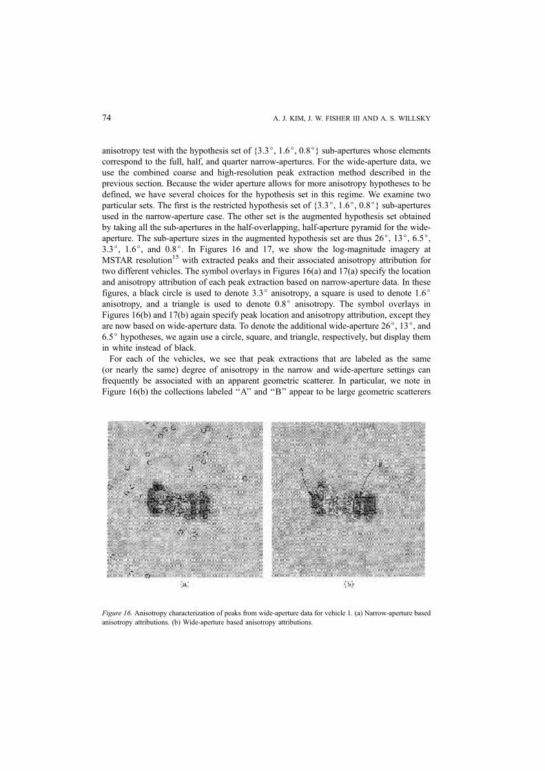
aperture. The sub-aperture sizes in the augmented hypothesis set are thus 26j, 13j, 6.5j,3.3j, 1.6j, and 0.8j. In Figures 16 and 17, we show the log-magnitude imagery at

MSTAR resolution15 with extracted peaks and their associated anisotropy attribution for

two different vehicles. The symbol overlays in Figures 16(a) and 17(a) specify the location

and anisotropy attribution of each peak extraction based on narrow-aperture data. In these

figures, a black circle is used to denote 3.3j anisotropy, a square is used to denote 1.6janisotropy, and a triangle is used to denote 0.8j anisotropy. The symbol overlays in

Figures 16(b) and 17(b) again specify peak location and anisotropy attribution, except they

are now based on wide-aperture data. To denote the additional wide-aperture 26j, 13j, and6.5j hypotheses, we again use a circle, square, and triangle, respectively, but display them

in white instead of black.

For each of the vehicles, we see that peak extractions that are labeled as the same

(or nearly the same) degree of anisotropy in the narrow and wide-aperture settings can

frequently be associated with an apparent geometric scatterer. In particular, we note in

Figure 16(b) the collections labeled ‘‘A’’ and ‘‘B’’ appear to be large geometric scatterers

Figure 16. Anisotropy characterization of peaks from wide-aperture data for vehicle 1. (a) Narrow-aperture based

anisotropy attributions. (b) Wide-aperture based anisotropy attributions.


at the front and rear of the vehicle and are appropriately characterized as anisotropic. Note

that based on the narrow-aperture data, the two scatterers labeled ‘‘A’’ are attributed as

3.3j in Figure 16(a), but there is no means of telling if the underlying scatterers are

actually 3.3j or perhaps less anisotropic since 3.3j is the lowest degree of anisotropy

available in the narrow-aperture setting. However, with the augmented hypothesis set for

wide-aperture data, we see that in fact they are both approximately 3.3j, and not much

more. This result demonstrates how the additional hypotheses afforded by the larger

aperture allow more anisotropy information to be conveyed for smaller scatterers. We also

point out that in Figures 16 and 17, those peak extractions which do not have the same

anisotropy attribution in the narrow and wide-aperture regime are frequently not identi-

fiable with a geometric scatterer and have a less anisotropic classification (usually the

minimally anisotropic 26j classification) in the wide-aperture setting.

So far, we have observed the conjectured benefit of wide-aperture data over narrow-

aperture data on the anisotropy characterization of geometric scatterers, i.e. the preserva-

tion of higher degrees of anisotropy in the narrow-aperture data and elaboration of the least

anisotropic narrow-aperture hypothesis by augmenting the hypothesis set with larger sub-

aperture hypotheses. This result is predicted by the analysis presented earlier. That analysis

also predicted a reduction in the rate of volumetric anisotropy as aperture size is increased.

To test this behavior with real data, we use the wide-aperture data focused on clutter using

26j and 3.3j apertures as before. In particular, we examine the three clutter scenes

composed of trees and field shown in Figure 18 where the narrow-aperture anisotropy

characterization is displayed in the left-hand side and the wide-aperture characterization is

displayed in the right-hand side. The set of hypotheses and respective graphical labels are

the same as in Figures 16 and 17. It is immediately clear that there is a significant

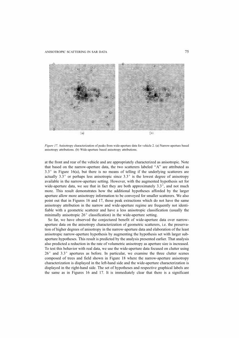
Figure 17. Anisotropy characterization of peaks from wide-aperture data for vehicle 2. (a) Narrow-aperture based

anisotropy attributions. (b) Wide-aperture based anisotropy attributions.


reduction in the rate of higher degrees of anisotropy using wide-aperture data. To explicitly

see that this reduction is due to the volumetric scatterers being resolved into individual

isotropic scatterers (in contrast to their simply being independently distributed over the

larger hypothesis set), we show in Tables 2 and 3 the tabulated anisotropy correspondences

Figure 18. Anisotropy characterization of peaks from 3 instances of clutter in the wide-aperture data. Left:

Narrow-aperture anisotropy attributions. Right: Wide-aperture anisotropy attributions.


between the two cases. Table 2 shows the correspondences between the narrow and wide-

aperture anisotropy classifications when both are restricted to use the same set of narrow-

aperture hypotheses. The empirical results here strongly argue that the wider aperture has

resolved the scatterers which were attributed as 1.6j and 0.8j under the narrow-aperture

into individual minimally anisotropic 3.3j scatterers. Table 3 shows the same as Table 2

except that the correspondences here are for when the augmented hypothesis set is used for

the wide-aperture data. Here we see that many of the 3.3j anisotropy classifications are

further resolved into the less anisotropic classifications and the majority of them are

assigned to the 26j minimal degree of anisotropy. Thus, we see the predicted reduction in

the rate of volumetric anisotropy in real wide-aperture data.

5. Conclusions

We have proposed a general characterization of anisotropy based on concentrated

scattering in azimuth. A sub-aperture pyramid is used to generate a tree of multi-resolution

images at a variety of cross-range versus azimuthal resolutions allowing for the detection

of anisotropic phenomena. With each sub-aperture in the pyramid, we associate a

hypothesis that the azimuthal scattering is confined to and uniform over that sub-aperture.

This model then leads to a sequence of hypothesis tests to characterize anisotropy which

can be approximated with an efficient pruning algorithm due to the tree-structure over the

sub-apertures.

This characterization of anisotropy allows us to explore some of the underlying

phenomenology behind anisotropic scattering. In particular, we study the canonical flat

plate and volumetric scatterer. Anisotropy plots clearly show a strong observability of the

Table 2. Anisotropy classification correspondences for

clutter with narrow and wide-aperture data using the

same anisotropy hypotheses.

Narrow-ap.\Wide-ap. 3.3j 1.6j 0.8j

3.3j 176 0 0

1.6j 45 0 1

0.8j 3 0 0

Table 3. Anisotropy classification correspondences for clutter with narrow and wide-

aperture data using the augmented hypothesis set for wide-aperture data.

Narrow-ap.\Wide-ap. 26j 13j 6.5j 3.3j 1.6j 0.8j

3.3j 117 28 10 15 3 3

1.6j 29 8 5 2 0 2

0.8j 1 2 0 0 0 0


inverse relation between plate size and degree of anisotropy that is predicted by physics-

based models. Anisotropy is also strongly dependent on the spatial distribution of a dense

cluster of isotropic scatterers composing a volumetric scatterer, however, as the density of

scatterers is reduced, this dependence decreases as the scatterers are more frequently

resolved into constituent isotropic scatterers. The dependence of volumetric anisotropy on

the density of the scatterers leads to the attribute that the probability of volumetric

anisotropy classifications can be reduced by increasing the size of the aperture. The only

significant effect on geometric anisotropy of extending the aperture is related to additional

hypotheses (corresponding to larger sub-apertures) in the augmented hypothesis set. In

particular, the larger sub-aperture hypotheses allow for a more accurate characterization of

smaller scatterers which exhibit broader (but still anisotropic over the wide-aperture)

azimuthal energy concentrations.

Besides demonstrating results on synthesized data, our anisotropy analysis is applied to

real data. Peaks are extracted from data and attributed with a degree of anisotropy. The

behavior of the peak attribution is consistent with the results of the synthetic data. In

particular, the anisotropy characterization of geometric scatterers is consistent between

narrow and wide-aperture settings when the underlying anisotropy is included in both

hypothesis sets. Furthermore, in the wide-aperture setting with the augmented hypothesis

set, we obtain a more detailed anisotropy characterization for smaller scatterers. A

reduction in the rate of volumetric anisotropy with larger apertures is also observed using

the real data.

The results presented here show a great deal of promise for the use of wide-aperture

data. This benefit does not necessarily arise from simply using higher resolution imagery

in existing ATR algorithms but comes from exploiting previously ignored anisotropy

information. Not only can this information aid existing algorithms by providing better

reflectivity estimates but also by characterizing scatterer stability as one can tell with more

confidence which peak extractions are due to stable geometric scattering. Furthermore, the

anisotropy information itself is a useful feature in ATR as this information allows one to

infer properties of the underlying scatterer geometry.

Appendix A. Anisotropy Statistic Accounting for Neighboring Scatterers

In this Appendix, we present the details in extending the isolated scatterer anisotropy test

to account for the presence of interfering scatterers by generalizing the model in Eq. (4) to

explicitly include multiple scatterers. First, however, we must generalize the sub-aperture

scattering model to account for the modulations produced by neighboring scatterers.

Again, we assume that the sub-aperture measurements have been formed while being

focused on a particular cross-range location y0. The possibility of other scatterers are

considered at discrete locations y0 þ k�p, where �p specifies a cross-range sampling

resolution for interfering scatterers. To model the effect of a scatterer with anisotropy

Hmk ;ik at location y0 þ k�p on the measurements at location y0, we simply modulate the

azimuthal response 1Hmk ;ikð�Þ to account for the shift in the image domain. The observed


effect over the smallest sub-apertures is then given by

bkðmk ; ikÞj ¼ZSM ; j

e j2pk�p

�rt1Hmk ;ik

ðtÞ dt ð11Þ

where �r is the null-to-null cross-range resolution associated with the full-aperture.

Incorporation of the neighboring scatterers is now modeled via superposition, i.e.

qM ¼Xk

Akbkðmk ; ikÞ þ e ð12Þ

where the noise model is the same as in Eq. (5). The summation over k in Eq. (12) should

be over a range large enough to include all scatterers contained in the coarsest resolution

cell, i.e. the resolution cell associated with the smallest sub-apertures. Thus, if L* is the

smallest aperture length, then we need to consider k 2 {�K, . . . , K} where

2K�p ��r

L*¼ size of coarest resolution cell

K � �r

2L*�p

� �ð13Þ

and k ¼ 0 corresponds to the resolution cell under investigation. Rewriting Eq. (12) as a

matrix equation we get

qM ¼ b�Kðm�K ; i�KÞ j : : : j bKðmK ; iKÞ� A�K

]AK

24

35þ e

¼ BAþ e ð14Þ

where B and A are appropriately defined16. Thus, we can use weighted least squares

(WLS) to implicitly estimate the values of the interfering Ak and account for their

contribution to qM. In order to have our least squared error minimization correspond to

ML, we weight our inner product by the inverse of the noise covariance to whiten the

measurements, i.e. hu;ui ¼ 12�2 uTL�1u . The ML estimate for A is obtained from this

model as

^A ¼ arg minA

fNeN2L�1g ¼ ðBVL�1BÞ�1

BVL�1qM

which simplifies to Eq. (6) in the case of limiting the model order to K ¼ 0. One

would like to then use ML to classify the anisotropy of the k ¼ 0 scatterer, i.e. choose

the sub-aperture hypothesis which minimizes the weighted norm of the estimated error

e ¼ qMz � B A . The model in Eq. (12), however, has too many reflectivity parameters

and thus results in an under-constrained minimization problem. In particular, if one


chooses K sufficiently large to account for all scatterers in the coarsest resolution cell,

then the model order is greater than the number of sub-aperture measurements and the

estimated e can be made zero for all hypotheses. Thus, we need to regularize the

model. In order for the estimated error e to be made small under the incorrect model,

many of the values in A generally have to be made unreasonably large and result in an

unrealistic scenario. Thus, we impose a 2-norm regularization penalty in the estimation

of A. In particular, instead of minimizing the weighted squared error to estimate A, we

take as our estimate

^A ¼ arg minA

fNeN2L�1 þ �AVRAg

¼ ðBVL�1Bþ �RÞ�1BVL�1qM

¼ PqM ð15Þ

where P is defined accordingly, � is the regularization parameter, and R is the regularization

matrix that penalizes the energy in all Ak other than k ¼ 0, i.e.

R ¼ I � eKeKV ¼ diagð1; . . . ; 1; 0; 1; . . . ; 1Þ:

This regularized estimate for A produces the following value for the weighted norm on the

error estimate

NeN2L�1 ¼ NqM � B ^AN2

L�1

¼ 1

2�2qMV

�L�1 � 2L�1BP þ PVBVL�1BP

qM ð16Þ

which can be used as the sufficient statistic ‘m,i for our hypothesis test as this statistic

corresponds to a generalized log-likelihood with a Gaussian prior on the neighboring

reflectivities.

Although the norm in Eq. (16) is a statistic which can be easily calculated, there are an

excessively large number of extended-hypotheses for which the test statistic needs to be

computed. In particular, if we allow 2K neighboring scatterers, the number of candidate

extended-hypotheses is now H2Kþ1 since each location has an associated scatterer and

corresponding anisotropy hypothesis. For the initial work presented in this paper, we

restrict our attention to hypotheses where only the anisotropy for the focused resolution

cell under investigation is allowed to vary. In particular, the hypothesis for each of the 2K

neighboring pixels is fixed to be full-aperture anisotropy while all hypotheses for the

focused location are tested. Thus, we escape the exponential growth in the number of

hypotheses since our hypothesis space is effectively still H. Certainly, this constraint can

be relaxed in order to appropriately take into account the anisotropy of neighboring

scatterers, but we do not do so here17. We make special note that although the model for

neighboring scatterers is restricted to full-aperture scattering, this multiple scatterer model


is more powerful than the isolated scatterer model presented in Section 3.1 as the latter

does not explicitly consider any interference from neighboring scatterers.

Notes

1. Correspondence should be sent to: Andrew Kim.

2. We will refer to anisotropy due to geometric scatterers as geometric anisotropy and anisotropy due to

volumetric scatterers as volumetric anisotropy.

3. For clarity, we will exclusively use the term ‘‘cross-range’’ when referring to cross-range in the spatial

(image) domain, and we will exclusively use the term ‘‘azimuthal’’ when referring to the corresponding

dimension in the sensor domain.

4. By azimuthal response, we mean the 1-D cross-range uncompressed signal for a given down-range location.

The signal a(t) is assumed to have already been appropriately demodulated to have zero phase modulation for

the inspected cross-range location.

5. The lack of normalization simplifies the notation in what follows later.

6. To be precise, it is actually the mean-squared reflectivity estimate normalized by the variance of the estimate

that decreases as too much of the aperture is used. The estimator variance itself actually decreases because the

coherent averaging is done over a larger aperture, but the squared-mean of the estimate decreases even more

so since no additional signal energy is being incorporated.

7. The details of the multiple scatterer model, and the derivation of the resulting statistic can be found in

Appendix A.

8. The term ‘‘sidelobes’’ here refers to those on a sinc-like function and not those associated a neighboring scatterer.

9. A comparison between the test based on the multiple scatterer model and the test from the isolated scattering

model can be found in Chapter 5 of Kim [8].

10. The hypotheses thus correspond to isotropic (i.e. constant over the full 2.8j aperture), half-aperture (1.4j),and quarter-aperture (0.7j) anisotropy.

11. These other ripples are too small to be seen on this plot but are apparent if the noise level is increased or the

scaling of the vertical axis is changed.

12. For each Monte Carlo trial, the peak extraction step detects local maximum in the log-magnitude reflectivity

image and refines the scattering center location using parabolic interpolation.

13. This sub-aperture pyramid does not have the full-aperture at the root, however, all the previous analysis in

Section 3 still applies. We note that the use of this ‘‘cropped’’ pyramid is solely to aid our comparison of

narrow and wide-aperture data. In applied settings, we recommend that the full-aperture always reside at the

root node to make maximum use of the aperture.

14. Note that there is also the issue of consistency of the peak locations. In order to overcome this problem, we

first estimate the coarse-resolution peak location and then limit the high-resolution peak location to reside

within the resolution cell corresponding to the coarse-resolution extraction.

15. The coarse resolution is used for the wide-aperture case (even though a finer imaging resolution can be

achieved) due to publishing restrictions on this data.

16. Although the matrix B clearly depends on the extended-hypothesis {(m�K, i�K), . . . , (mK, iK)}, this

dependence is omitted for notational simplicity.

17. Research along this direction can be found in Chapter 7 of the thesis by Kim [8].

References

1. M. Allen, D. Sofianos, and L. Hoff, ‘‘Wide-Angle Wideband SAR Matched Filter Image Formation for

Enhanced Detection Performance,’’ in Proc. of the SPIE, Algorithms for SAR Imagery, vol. 2230, Apr. 1994,

pp. 302–314.


2. R. Chaney, A. Willsky, and L. Novak, ‘‘Coherent Aspect-Dependent SAR Image Formation,’’ in Proc. of the

SPIE, Algorithms for SAR Imagery, vol. 2230, Apr. 1994, pp. 256–274.

3. J. Capon, ‘‘High-Resolution Frequency-Wavenumber Spectrum Analysis,’’ in Proc. IEEE, vol. 57, no. 8,

Aug. 1969, pp. 1408–1418.

4. G. Benitz, ‘‘Adaptive High-Definition Imaging,’’ in Proc. of the SPIE, Algorithms for SAR Imagery, vol.

2230, Apr. 1994, pp. 106–119.

5. G. Benitz and D. DeLong, ‘‘Extensions of High Definition Imaging,’’ in Proc. of the SPIE, Algorithms for

SAR Imagery, vol. 2487, Apr. 1995, pp. 165–180.

6. ‘‘MSTAR (Public) Targets: T-72, BMP-2, BTR-70, SLICY’’, see http://www.mbvlab.wpafb.af.mil/public/

MBVDATA.

7. A. Kim, Exploring Scatterer Anisotropy in Synthetic Aperture Radar via Sub-Aperture Analysis, PhD thesis,

Massachusetts Institute of Technology, Sept. 2001.

8. A. Kim, J. Fisher, A. Willsky, and P. Viola, ‘‘Nonparametric Estimation of Aspect Dependence for ATR,’’ in

Proc. of the SPIE, Algorithms for SAR Imagery, vol. 3721, Apr. 1999, pp. 332–342.

9. H. Chiang and R. Moses, ‘‘ATR Performance Prediction Using Attributed Scattering Features,’’ in Proc. of

the SPIE, Algorithms for SAR Imagery, vol. 3721, Apr. 1999, pp. 785–796.

10. A. Kim, S. Dogan, J. Fisher, R. Moses, and A. Willsky, ‘‘Attributing Scatterer Anisotropy for Model Based

ATR,’’ in Proc. of the SPIE, Algorithms for SAR Imagery, vol. 4053, Apr. 2000.

11. L. Potter and R. Moses, ‘‘Attributed Scattering Centers for SAR ATR,’’ IEEE Trans. on Image Proc., vol. 5,

Jan. 1997, pp.79–91.


Detection and Analysis of Anisotropic Scattering in SAR...

Documents

Transcript of Detection and Analysis of Anisotropic Scattering in SAR...