Detecting the Schumann Resonances - Tesla Radio · Scott Fusare 8/22/01 An experimenters approach...
5
Scott Fusare 8/22/01 An experimenters approach to detecting the Schumann Resonances The earth / ionosphere wave guide resonances were first predicted and mathematically described in 1952 by W. O. Schumann, the man who’s name is now synonymous with the phenomenon. He also became the first to report in open literature the experimental detection of this phenomenon (1954). Much conjecture has occurred as to whether Tesla was aware of, and able to utilize, the earth / ionosphere cavity resonance. I tend to believe he did not, but that issue continues to be a contentious one. Presented here is a relatively simple means for the amateur experimenter to monitor the Schumann resonances. The Schumann resonances manifest themselves as spectral peaks in the natural background EM noise levels. Most easily detected are the first 4 “modes” which occur at roughly 7.8 Hz, 14 Hz, 20 Hz and 26 Hz. The signal levels involved fall into the low picoTesla / microvolt range. As the mode order increases, signal strength decreases. Most “professionals” monitor the magnetic component of the peaks using large induction coils. This method has the advantage of being immune to the ambient weather conditions (the coils are often buried), easy to calibrate and suffering from lower levels of man made and natural interferance. Unfortunately, to have the required sensitivity at the frequencies of interest, the sensor coils must either be physically large in area, contain a huge number of turns or be wound on special very high permeability cores. Recall that the voltage induced on a coil by a time varying magnetic field is V = ωANB and the problem becomes apparent. Although this method is surely not beyond the means of ambitious experimenters (see, for example, www.vlf.it/inductor/inductor.htm) it is tedious and potentially expensive. For those having shallow pockets (me), or lacking the resolve to construct such a massive coil (me again), detecting the vertical E-field component of the Schumann resonances gives a workable, if somewhat less robust, option. The hardware is relatively simply and the antenna small, a 2 meter whip. In the realm of VLF/ELF signals, antennas are always electrically short (< 1/10 λ). In our case the antenna is vanishingly short, 1/4 λ at 8 Hz is ~9400 Km !. Under these circumstances the antenna can be thought of as a capacitor, equal in value to the isotropic capacity of the antenna, in series with a voltage generator representing the signal. The magnitude of this voltage generator will be the product of the incident wave field strength and the effective height of the antenna. A well insulated 2 meter whip reasonably remote from surrounding objects should develop 1 - 10 µV of signal at the first Schumann peak.
Transcript of Detecting the Schumann Resonances - Tesla Radio · Scott Fusare 8/22/01 An experimenters approach...

Scott Fusare 8/22/01
An experimenters approach to detecting the SchumannResonances
The earth / ionosphere wave guide resonances were first predicted andmathematically described in 1952 by W. O. Schumann, the man who’s name is nowsynonymous with the phenomenon. He also became the first to report in open literaturethe experimental detection of this phenomenon (1954). Much conjecture has occurred asto whether Tesla was aware of, and able to utilize, the earth / ionosphere cavityresonance. I tend to believe he did not, but that issue continues to be a contentious one.Presented here is a relatively simple means for the amateur experimenter to monitor theSchumann resonances.
The Schumann resonances manifest themselves as spectral peaks in the naturalbackground EM noise levels. Most easily detected are the first 4 “modes” which occur atroughly 7.8 Hz, 14 Hz, 20 Hz and 26 Hz. The signal levels involved fall into the lowpicoTesla / microvolt range. As the mode order increases, signal strength decreases.
Most “professionals” monitor the magnetic component of the peaks using largeinduction coils. This method has the advantage of being immune to the ambient weatherconditions (the coils are often buried), easy to calibrate and suffering from lower levels ofman made and natural interferance. Unfortunately, to have the required sensitivity at thefrequencies of interest, the sensor coils must either be physically large in area, contain ahuge number of turns or be wound on special very high permeability cores. Recall thatthe voltage induced on a coil by a time varying magnetic field is V = ωANB and theproblem becomes apparent. Although this method is surely not beyond the means ofambitious experimenters (see, for example, www.vlf.it/inductor/inductor.htm) it is tedious andpotentially expensive. For those having shallow pockets (me), or lacking the resolve toconstruct such a massive coil (me again), detecting the vertical E-field component of theSchumann resonances gives a workable, if somewhat less robust, option. The hardware isrelatively simply and the antenna small, a 2 meter whip.
In the realm of VLF/ELF signals, antennas are always electrically short (< 1/10λ). In our case the antenna is vanishingly short, 1/4 λ at 8 Hz is ~9400 Km !. Under thesecircumstances the antenna can be thought of as a capacitor, equal in value to the isotropiccapacity of the antenna, in series with a voltage generator representing the signal. Themagnitude of this voltage generator will be the product of the incident wave field strengthand the effective height of the antenna. A well insulated 2 meter whip reasonably remotefrom surrounding objects should develop 1 - 10 µV of signal at the first Schumann peak.
Scott Fusare 8/22/01
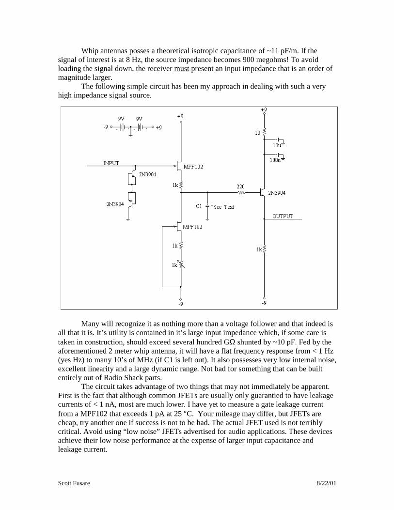
Whip antennas posses a theoretical isotropic capacitance of ~11 pF/m. If thesignal of interest is at 8 Hz, the source impedance becomes 900 megohms! To avoidloading the signal down, the receiver must present an input impedance that is an order ofmagnitude larger.
The following simple circuit has been my approach in dealing with such a veryhigh impedance signal source.
Many will recognize it as nothing more than a voltage follower and that indeed isall that it is. It’s utility is contained in it’s large input impedance which, if some care istaken in construction, should exceed several hundred GΩ shunted by ~10 pF. Fed by theaforementioned 2 meter whip antenna, it will have a flat frequency response from < 1 Hz(yes Hz) to many 10’s of MHz (if C1 is left out). It also possesses very low internal noise,excellent linearity and a large dynamic range. Not bad for something that can be builtentirely out of Radio Shack parts.
The circuit takes advantage of two things that may not immediately be apparent.First is the fact that although common JFETs are usually only guarantied to have leakagecurrents of < 1 nA, most are much lower. I have yet to measure a gate leakage currentfrom a MPF102 that exceeds 1 pA at 25 °C. Your mileage may differ, but JFETs arecheap, try another one if success is not to be had. The actual JFET used is not terriblycritical. Avoid using “low noise” JFETs advertised for audio applications. These devicesachieve their low noise performance at the expense of larger input capacitance andleakage current.
Scott Fusare 8/22/01
The other advantage is secured by pressing into service the V/I characteristics of acommon NPN transistor’s base collector junction. If configured as shown, the pair willapproximate a very high value resistor. The predicted value for 2N3904 pair is a linear500 GΩ. In my experience it is not entirely linear and somewhat lower in value ~200GΩ. This is, however, more than adequate for our purposes. A word of caution, some ofthese transistors are gold doped which will make them unacceptable for this applicationbut I have yet to encounter this problem. As with the JFETs, these bipolars are verycheap, try some from another manufacturer if you have trouble. As an aside, if youhappen to actually have on hand a 10 GΩ, or larger, resistor by all means use it. It willhave lower noise and lower capacitance than the bipolar pair.
Construction is non-critical with the exception of a few rules that must beobserved.
1) Use a shielded enclosure.2) Do NOT insert the gate lead of the input JFET into the circuit board,
solder it directly to the input connector.3) Don’t scrimp on the input connector. What you use is up to you, but it
must have an excellent dielectric. Teflon is best, most other modernplastics are OK. Phenolic is completely unacceptable at this impedance. Iuse either SO-239 or BNC, both of which are commonly available withTeflon insulation.
4) Avoid touching the input connector insulation or the base of the inputJFET. It takes very little contamination to lower the impedance. Clean itwith distilled water and pure alcohol if things go awry.
Tune up is simple. Ground the input and adjust the trimmer for zero volts at theoutput. A few inches of wire inserted into the input should pick up 100s of mV of AChum and easily detect a piece of charged plastic waved around a few feet away.
The next problem becomes that of separating the desired signal from variousforms of natural and man made interference that will be easily 60 dB or more higher thanthe signal. Local AM stations, military VLF transmitters, powerful VLF lightning energyand power line interference are some of what must be contended with. Removing C1 andhooking the follower up to a scope, especially with FFT capability, is entertaining. Thefollower makes a great active antenna at VLF, even with it’s unity voltage gain. Anyway,most interference can be reduced to acceptable levels, or entirely eliminated with goodlow pass filtering. Setting the value of C1 to 270 nF will dramatically reduce theunwanted higher frequency crap. As the circuit is sensitive to frequencies below thatwhich we are interested in, it pays to use some high pass filtering also. Most problematicto deal with will the 60 Hz noise. Sharp low pass and notch filters will help, but this isvery dependent on the location. Some folks may find it impossible to remove enough ofthe 60 Hz energy at their location. The only alternative then becomes seeking a locationthat is electrically quieter. The actual filter configuration used will be dependent onindividual needs.
Last in the signal chain, some amplification of the filtered signal will be needed.The amount used will depend on the device being used to perform the spectral analysisand it’s input dynamic range. The amount tolerated will be predicated on the resultant
Scott Fusare 8/22/01
levels of 60 Hz energy after filtering. The output signal must not clip as information willbe lost and the FFT will generate bogus data. At my location a gain of 100 seems to be agood all around value.
Finally some means of performing spectral analysis of the signal are needed. Thisis usually done using a ADC and a Fast Fourier Transform or FFT algorithm. Althoughonce relegated to the realm of high-end test equipment, FFT capability is now common. Iuse a digital oscilloscope that has a FFT function built in. Less expensive options are nowcommonly available from companies such as Pico Technologies and Dataq. In fact, as ofthis writing (8/22/01) I see Dataq has a “start up” kit for $15. It boasts 4 channels with 8bit resolution at 240 samples per second, certainly adequate for this application(www.dataq.com/cgi-local/SoftCart.exe/115.htm). For those that wish to spend no cash, aPC sound card can and will work with limited flexibility. There are several freewaresoundcard FFT programs available.
Choose an antenna location as far from power lines and surrounding object aspractical. Nearby objects, such as trees, will form a capacitive voltage divider with theantenna and lower the signal, often dramatically. Monitoring during foul weather will befutile due to wind-induced signals, charge pulses from raindrops and the often badlyagitated natural electric field. Don’t forget to ground reference the follower!
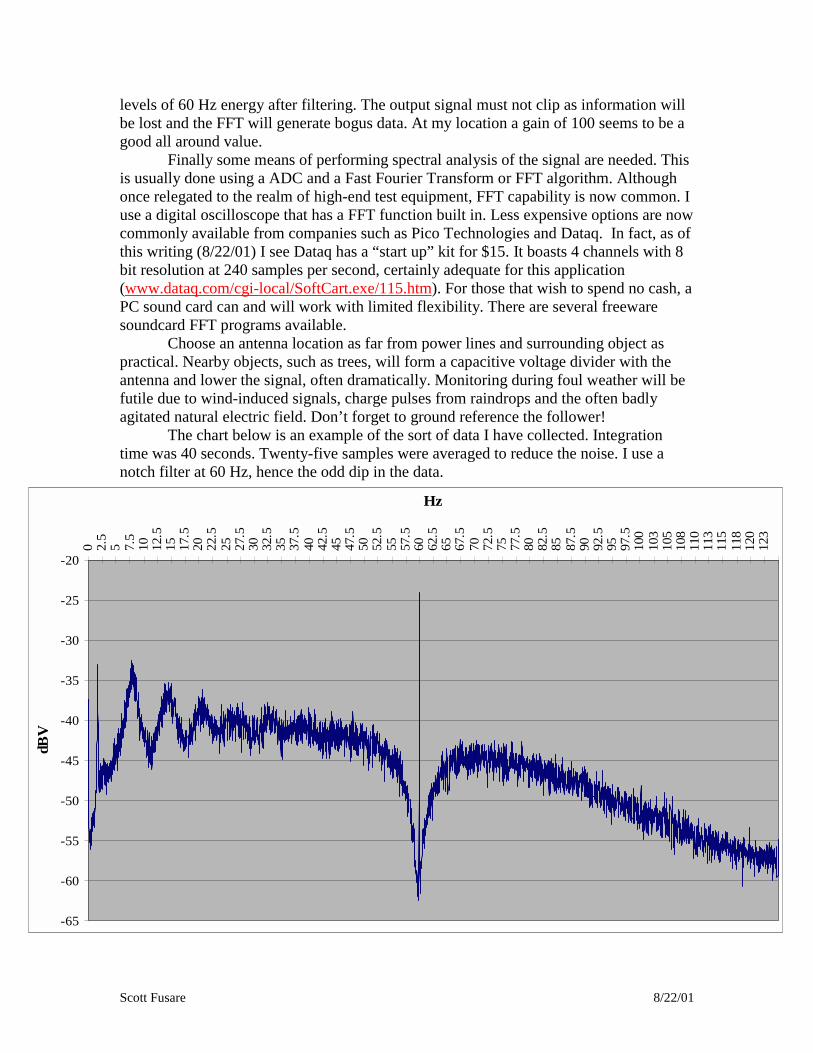
The chart below is an example of the sort of data I have collected. Integrationtime was 40 seconds. Twenty-five samples were averaged to reduce the noise. I use anotch filter at 60 Hz, hence the odd dip in the data.
-65
-60
-55
-50
-45
-40
-35
-30
-25
-20
0 2.5
5 7.5
10 12.5
15 17.5
20 22.5
25 27.5
30 32.5
35 37.5
40 42.5
45 47.5
50 52.5
55 57.5
60 62.5
65 67.5
70 72.5
75 77.5
80 82.5
85 87.5
90 92.5
95 97.5
100
103
105
108
110
113
115
118
120
123
Hz
dBV

Scott Fusare 8/22/01
This paper was written in haste and as such will likely contain errors and also befound devoid of certain details. I am more than willing to answer questions for those thatwould seriously attempt to duplicate this project. Please address any correspondence [email protected]