Detecting the Best Seasonal ARIMA Forecasting Model for ...

Yayın Geliş Tarihi: 25.10.2016 Dokuz Eylül Üniversitesi

Yayın Kabul Tarihi: 18.06.2017 …İktisadi ve İdari Bilimler Fakültesi Dergisi Online Yayın Tarihi: 04.12.2017 Cilt:32, Sayı:2, Yıl:2017, ss. 143-182

Detecting the Best Seasonal ARIMA Forecasting Model for Monthly

Inflation Rates in Turkey12

Mehmet ÖZMEN3 Sera ŞANLI4

Abstract

In this study, it has been aimed to find the best ‘Seasonal Autoregressive Integrated

Moving Average (SARIMA)’ model for monthly inflation rates for Turkish economy over the

period 1995:01-2015:03. Before the model identification based on Box Jenkins methodology,

HEGY monthly seasonal unit root test has been applied. The orders of seasonal differencing

have been detected through OCSB and CH tests. Finally, ARIMA(1,1,1)(1,0,2)[12] with drift

model chosen by using stepwise selection method and ARIMA(1,1,1)(2,0,0)[12] with drift

model chosen by using non-stepwise selection have been compared. The results have shown

that the former model is better as the best fitted SARIMA model.

Keywords: Inflation, Box Jenkins, SARIMA, HEGY, OCSB, CH, Stepwise Selection.

JEL Classification Codes: C01, C22, C51, E31.

Türkiye İçin Enflasyon Oranının Uygun Mevsimsel ARIMA Modeli

İle Belirlenmesi

Öz

Bu çalışmada Türkiye’nin 1995:01-2015:03 dönemine ilişkin aylık enflasyon oranları

için en iyi ‘Mevsimsel Otoregresif Bütünleşik Hareketli Ortalama (SARIMA)’ modelini

bulmak amaçlanmıştır. Box Jenkins metodolojisine dayalı model tanımlamasından önce

HEGY mevsimsel birim kök testi uygulanmıştır. Mevsimsel fark alma dereceleri OCSB ve CH

testleri kullanılarak saptanmıştır. Son olarak, sırasıyla adımsal (stepwise) ve adımsal

olmayan (non-stepwise) seçim yöntemleri kullanılarak seçilen sürüklenmeli

ARIMA(1,1,1)(1,0,2)[12] ve ARIMA(1,1,1)(2,0,0)[12] modelleri karşılaştırılmıştır. Sonuçlar

adımsal yöntem kullanılarak seçilen sürüklenmeli ARIMA(1,1,1)(1,0,2)[12] modelinin en iyi

uyan SARIMA modelini belirlemede adımsal olmayan modele göre daha iyi olduğunu

göstermiştir.

Anahtar Kelimeler: Enflasyon, Box Jenkins, SARIMA, HEGY, OCSB, CH, Adımsal

Seçim.

JEL Sınıflandırma Kodları: C01, C22, C51, E31.

1 This study has been derived from the Master Thesis that has been prepared in

consultancy of Assoc. Prof. Mehmet Ozmen called “The Econometric Analysis of Seasonal

Time Series: Applications on Some Macroeconomic Variables (Sanlı, 2015)”. 2 This study has been supported by TUBITAK (The Scientific and Technological

Research Council of Turkey) – BIDEB (Scientist Support Department) within the scope of

2211-E Direct National Scholarship Programme for PhD Students. 3 Prof. Dr., Çukurova Üniversitesi, İktisadi ve İdari Bilimler Fakültesi, Ekonometri

Bölümü, [email protected] 4 Arş. Gör., Çukurova Üniversitesi, İktisadi ve İdari Bilimler Fakültesi, Ekonometri

Bölümü, [email protected]

M.ÖZMEN – S. ŞANLI

144

1. INTRODUCTION

In terms of policy makers, it is of great importance to have a reliable inflation

rate forecast. In this context, the most suitable model should be accessed using

‘Seasonal Autoregressive Integrated Moving Average (SARIMA)’. Since SARIMA

models reveal more effective results in terms of handling the seasonal component of

the series apart from the non-seasonal one when compared to the traditional ARIMA

models. In this application, it has been aimed to find the best model for monthly

inflation rates and therefore monthly (seasonally unadjusted) consumer price index

(CPI) data have been utilized for Turkish economy over the period 1995:01-2015:03.

In modelling monthly inflation rates that are very crucial to design effective

economic strategies, choosing a suitable seasonal ARIMA model which includes

both seasonal and non-seasonal behaviours is not an easy task. Since such models

give point to the recent past rather than distant past, primarily they are convenient

for short term forecasting and this implies that long-term forecasts from ARIMA

models are less reliable than short term forecasts (Aidoo, 2010: 3).

The study of Canova and Hansen (1995) presents Lagrange Multiplier (LM) tests

of the null hypothesis of no unit roots at seasonal frequencies denoting the presence

of deterministic seasonality contrary to the tests of Dickey, Hasza and Fuller (DHF)

(1984) and Hylleberg, Engle, Granger and Yoo (HEGY) (1990) tests dealing with

the null of presence of seasonal unit roots. They generalize the Kwiatkowski,

Phillips, Schmidt, and Shin (KPSS) (1992) test framework.

Tam and Reinsel (1997) examine the locally best invariant unbiased (LBIU) and

point optimal invariant test procedures for a unit root in the seasonal moving average

(SMA) operator for SARIMA and make use of the monthly non-agricultural industry

employment series for males age 16-19 modelled by Hillmer, Bell and Tiao (1983).

The results for conducted simulations have revealed that for this series, seasonality

is stochastic and therefore seasonal differencing is appropriate. They also apply their

tests to different types of seasonal time series data and find some of these series to

have deterministic seasonality.

Dokuz Eylül Üniversitesi İktisadi ve İdari Bilimler Fakültesi Dergisi Cilt:32, Sayı:2, Yıl:2017, ss. 143-182

145

In the study by Lim and McAleer (2000), the presence of stochastic seasonality

is examined to clarify the nonstationary quarterly international tourist arrivals from

Hong Kong and Singapore to Australia from 1975:Q1 to 1996:Q4 using HEGY

(1990) procedure. Since the presence of seasonal unit roots gives an insight into a

varying seasonal pattern that is against a constant seasonal pattern, the Box Jenkins

SARIMA process is possible to be a more suitable model for tourist arrivals rather

than a deterministic seasonal model with seasonal dummy variables.

Cosar (2006) has tried to examine the seasonal properties of the Turkish CPI

through Beaulieu and Miron’s (1993) extension of the classical HEGY test

developed by Hylleberg et al. (1990) and the LM-type CH seasonal unit root test

procedures with the aim to specify the seasonality accurately in econometric models.

In Cosar’s (2006) study, there has been an evidence of both deterministic and

nonstationary stochastic seasonality in the CPI series of Turkey.

In their paper, Chang and Liao (2010) have aimed to forecast the monthly

outbound tourism departures of three major destinations from Taiwan to Hong Kong,

Japan and U.S.A. respectively using the SARIMA model.

Saz (2011) examines the efficacy of SARIMA models for forecasting Turkish

inflation rates from 2003 to 2009 and presents a methodological approach for a

combination of a systematic SARIMA forecasting structure and the stepwise

selection procedure of the Hyndman-Khandakar (HK) algorithm. This combination

is expressed to give rise to choosing a best single SARIMA model which is

SARIMA(0,0,0)(1,1,1) model with one degree of seasonal integration, one seasonal

autoregressive (AR) and one seasonal moving average (MA) part. According to a

structural break analysis, the Turkish inflation rates have been found to display a

range of structural breaks with the latest being in mid-2003 and stochastic nature of

Turkish inflation has been found to outweigh its deterministic nature.

Our study has mainly focused on searching for the best-fitted SARIMA model

for the monthly inflation rates in order to provide the best forecast. Therefore,

following the Box-Jenkins approach, in the application part first model identification


146

and estimation of parameters will be presented. Subsequent to this, diagnostic

checking results based on the residuals of the possible model will be given place in

order to make certain about the white-noise characteristic of residuals which

becomes a vital assumption for a good ARIMA model.

The rest of this paper has been organized as follows: Section 2 provides the

background for the analytical approach to SARIMA models, Beaulieu and Miron’s

(1993) extension of the classical HEGY test, OCSB and CH test; section 3 gives the

information about the data set and discussions on the empirical results. Finally,

section 4 presents the conclusions.

2. THEORETICAL BACKGROUND

2.1. Seasonal ARIMA Models (SARIMA)

The characterization of seasonal series occurs by a strong serial correlation at the

seasonal lag. As known, the classical decomposition of the time series consists of a

trend component, a seasonal component and a random noise component. But, in

practice it may not be logical to assume that the seasonality component repeats itself

exactly in the same way cycle after cycle. SARIMA models allow for randomness

in the seasonal pattern from one cycle to the next (Brockwell and Davis, 2006: 320).

Box and Jenkins (1970) present an extension of the ARIMA model in order to

take seasonal effects into consideration. At the core of idea, trying to adjust a cyclical

effect takes place for adding this seasonal component. For example, in the case of

monthly data, the observation may depend in part on accounting for an

annual effect. In the same manner, for daily data, the dependence may be realized

through representing a weekly effect. Coping with these dependencies in order

to remove the seasonal effect in question may be possible via differencing the data.

However, one can also specify AR or MA relationships at the seasonal interval in

question. For this case, Box and Jenkins (1970) define a general multiplicative

SARIMA model shown as ARIMA x , where the lower-case

letters indicate the nonseasonal orders and the upper-case letters

ty 12ty

7ty

),,( qdp sQDP ),,(

qdp ,, QDP ,,


147

indicate the seasonal orders of the process with period s (that is, s is the number of

observations per year). The parentheses mean that the seasonal and nonseasonal

elements are multiplied (Hamaker and Dolan, 2009: 198-199; Pankratz, 1983: 281).

Before giving a clear definition for SARIMA, assume that tX

,........)2,1,0( t is an ARMA ),( qp process if }{ tX is stationary and if for

every t,

qtqttptptt ZZZXXX .................... 1111 (1)

where ~ . (1) can be written symbolically as

tt ZLXL )()( , ,........)2,1,0( t (2)

where and are the and degree polynomials

ppzzz .........1)( 1 (3)

and

qqzzz .........1)( 1 (4)

and L is the backward shift operator defined by jttj XXL ,

,........2,1,0 j . These and polynomials are mentioned as the AR and MA

polynomials respectively of the difference equations (2) (Brockwell and Davis,

2006: 78). If we fit an ARMA ),( qp model tt ZLYL )()( to the differenced

series tS

t XLY )1( , then the model for the original series becomes

ttS ZLXLL )()1)(( . This is a special case of the general SARIMA model

which will be defined as follows:

Definition: If d and D are nonnegative integers, then { } is a seasonal ARIMA

x process with period s if the differenced series

tDSd

t XLLY )1()1( is a causal ARMA process defined

}{ tZ ),0( 2WN

thp thq

tX

),,( qdp sQDP ),,(


148

tS

tS ZLLYLL )()()()( , }{ tZ ~ ),0( 2WN (5)

where P

Pzzz .........1)( 1 (seasonal AR(P) characteristic

polynomial), Q

Qzzz .........1)( 1 (seasonal MA(Q) characteristic

polynomial) with )(z and )(z expressed in (3) and (4) respectively (Brockwell

and Davis, 2002: 203). On the other hand, a more general multiplicative SARIMA

model can be expressed by adding a constant term to take the case of a

deterministic trend into consideration as follows:

tS

tS ZLLYLL )()()()( (6)

and substituting tdD

StDSd

t XXLLY )1()1( into (6), it becomes

tS

tdD

SS ZLLXLL )()()()( (7)

(Shumway and Stoffer, 2011: 157).

As seen in the definition given above, derivation of }{ tY comes from the original

series }{ tX using both simple differencing (in order to remove trend) and seasonal

differencing S

S L 1 to remove seasonality. For instance, when 1Dd and

12s , then tY becomes

1121212 tttt XXXY )()( 13112 tttt XXXX (8)

Now take a SARIMA model of order x . Then this model can be

written in the following equation:

tt ZLYL )1()1( 12 (9)

where tt XY 12 . Then we find

1213112 )( tttttt ZZXXXX (10)

)0,0,1( 12)1,1,0(


149

so that depends on and as well as the innovation at time

(Chatfield, 1996: 60).

Now let us take an ARIMA x process with a periodicity of length

12 (since, s=12). In this example, it is obvious that tX does not require seasonal and

nonseasonal differencing at all since 0d and 0D . On the other hand, the

seasonal part of the process is composed of one AR )1( P and one MA )1( Q

component at lag 12. In addition, there is a nonseasonal AR term at lag 1 )1( p .

The multiplication of the two AR operators in the lag operator form can be expressed

as

tt ZLXLL )1()1)(1( 121

1211 (11)

(Pankratz, 1983: 281).

In identifying SARIMA model, the first task is to find values d and D which

reduce the series to stationarity and remove most of the seasonality. Then, we need

to assess the values of and by examining the sample autocorrelation

function (ACF) and partial autocorrelation function (PACF) of the differenced series

at lags which are multiples of s and choosing a SARIMA model in which ACF and

PACF have a similar shape. Ultimately, the model parameters may be estimated

through an appropriate iterative procedure. For details, see Box and Jenkins (1970,

chap. 9) (Chatfield, 1996,: 60-61) (all AR and MA polynomial representations have

been taken from Brockwell and Davis, 2006: 78).

2.1.1. Stationarity and Invertibility Conditions

Representing a model in a multiplicative form is a big convenience in terms of

expressing the seasonal and nonseasonal components separately and controlling the

stationarity and invertibility conditions. For instance, take an ARIMA x

model and express it in a lag operator form as follows:

tX 121, tt XX 13tX

)12( t

)0,0,1( 12)1,0,1(

qPp ,, Q

)1,0,2(

s)2,0,1(


150

tss

ts ZLLLXLLL )1)(1()1)(1( 1

2211

221 (12)

The stationary requirement applies only to the AR coefficients. The nonseasonal

part of (12) has the same stationarity conditions as for an )2(AR :

and . Now we need to apply a seperate stationary condition

for the AR seasonal part. It is the same as for a nonseasonal AR(1) model, except in

this case we have a seasonal sAR )1( component; so the condition becomes 11

.

As in the case of stationarity, we need to consider invertibility condition which

applies only to the MA part of (12) for nonseasonal and seasonal components

separately. For the nonseasonal part, the condition is . The conditions on the

seasonal part are the same as for a nonseasonal MA(2) model, except in this case

there exists an sMA )2( component. Therefore the joint conditions are given as

12 , 112 and 112 (Pankratz, 1983: 285). (AR and MA

polynomial representations have been taken from Brockwell and Davis, 2006: 78).

2.1.2. The Expanded Model

It should be noted that all multiplicative SARIMA models can be telescoped into

an ordinary ARMA model in the variable

tdD

S

def

t XY (13)

For instance, consider that the series Tttx 1}{ follows a SARIMA x

or ARIMA x 12)1,1,0( model. For this process, we have

tt ZLLXLL )1)(1()1)(1( 1211

12 (14)

and it becomes

,12

,112 112

11

),( qp

)1,1,0(

)1,1,0,12( )1,1,0(


151

tt ZLLLY )1( 1311

1211 (15)

where . Hence, it can be said that this multiplicative

SARIMA model has an ARMA (0,13) representation where only the coefficients 1

, 112 def

and 1113 def

are not zero and all other coefficients of the MA

polynomial are equal to zero. So, if the model in question is SARIMA x

given in (14), only the two coefficients which are and 1 have to be

estimated. However, for the ARMA (0,13), instead we have to estimate the three

coefficients which are , and . Therefore, it is apparent that SARIMA

models take a parsimonious model structure into account and a model specification

such as (15) is called an expanded model. In addition, we can say that only an

expanded multiplicative model can be estimated directly (Chen, Schulz and Stephan,

2003: 233-234).

2.1.3. Theoretical ACFs and PACFs for Seasonal Processes

In SARIMA models, estimated acfs and pacfs display the same expected

behaviours as in the structure of nonseasonal models. For seasonal time series data,

observations s time periods apart have characteristics

in common. So, observations s periods apart are expected to be correlated and in this

manner, acfs and pacfs for seasonal series should have nonzero coefficients at one

or more multiples of lag s . If we observe nonseasonal and purely

seasonal acfs and pacfs, it is seen that the coefficients appearing at lags 1,2,…. in the

former appear at lags in the latter.

This similarity between nonseasonal and seasonal acfs and pacfs makes the

seasonal analysis simpler. So, having knowledge of nonseasonal acfs and pacfs helps

give a description of identical patterns occurring at multiples of lag s (Pankratz,

1983: 270-271). For more details, see Box and Jenkins (1976, chap. 9).

tt XLLY )1)(1( 12

)1,1,0(

)1,1,0,12( 1

1 12 13

,.....),,,,( 22 ststststt zzzzz

,......)3,2,( sss

,......3,2, sss


152

2.2. Testing for Seasonal Unit Roots in Monthly Data

Beaulieu and Miron (1992) make an extension of HEGY testing procedure for

monthly data. )(* L is a polynomial associated with roots that are outside the unit

circle and it can be expressed as

12

11,13

*)(k

ttkkt yyL (16)

where,

tt yLLLLLLLLLLLy )1( 111098765432,1 (17)

tt yLLLLLLLLLLLy )1( 111098765432,2 (18)

tt yLLLLLLy )( 119753,3 (19)

tt yLLLLLy )1( 108642,4 (20)

tt yLLLLLLLLLLLy )22221(2

1 111098765432,5 (21)

tt yLLLLLLLy )1(2

3 1097643,6 (22)

tt yLLLLLLLLLLLy )22221(2

1 111098765432,7 (23)

tt yLLLLLLLy )1(2

3 1097643,8 (24)

tt yLLLLLLLLLy )233233(2

1 1110976543,9 (25)


153


1 109876432,10 (26)


1 1110976543,11 (27)


1 109876432,12 (28)

tt yLy )1( 12,13 (29)

(Beaulieu and Miron, 1992: 2-4).

With these transformations ( ,iy s) of ty , the seasonal unit roots are excluded at

given frequencies while they are preserved at remaining frequencies. To give an

example, consider the ty1 transformation. While it eliminates the seasonal unit roots,

it preserves the long-run or zero frequency unit root. In table 1, the outline of long

run and seasonal frequencies has been presented:


154

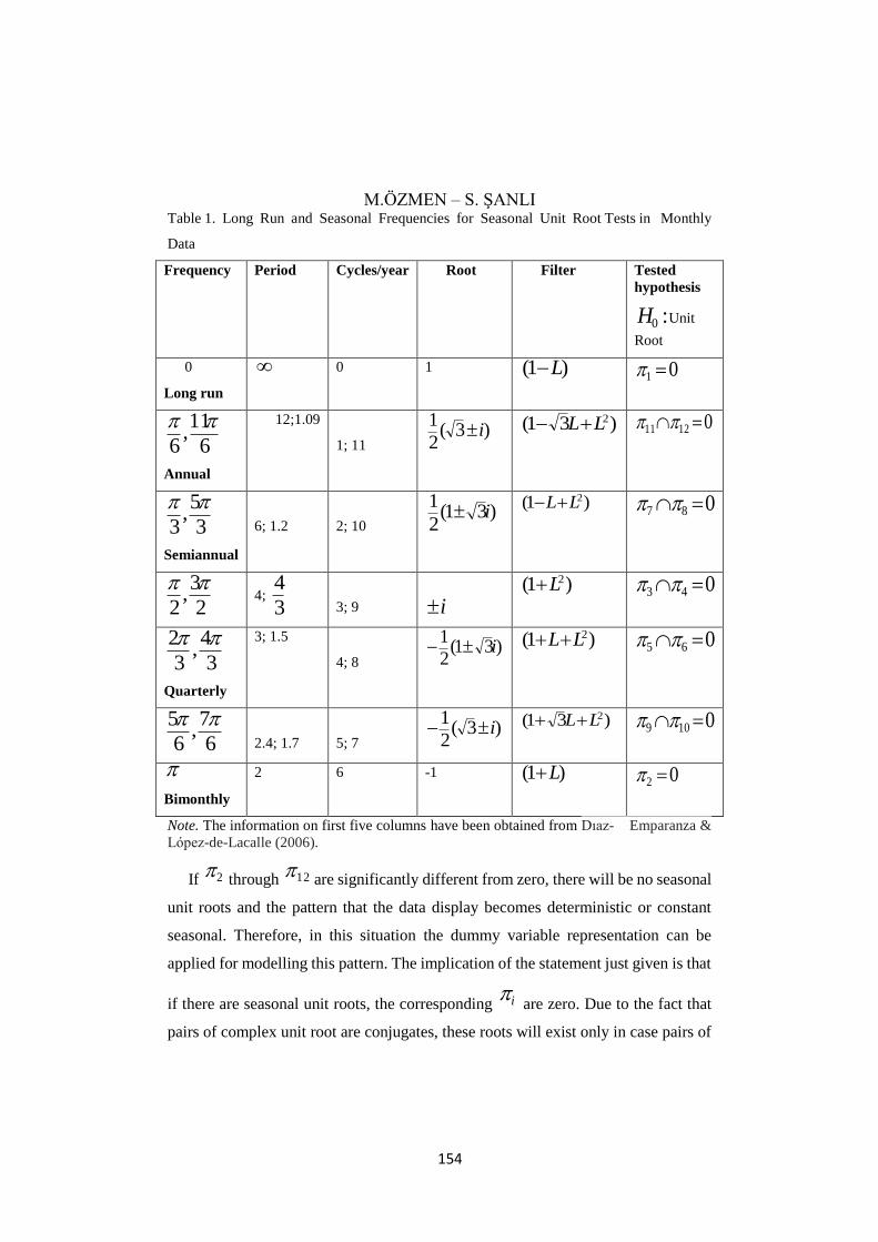
Table 1. Long Run and Seasonal Frequencies for Seasonal Unit Root Tests in Monthly

Data

Frequency Period Cycles/year Root Filter Tested

hypothesis

:0H Unit

Root

0

Long run

0 1 )1( L 01

6

11,

6

Annual

12;1.09

1; 11 )3(

2

1i )31( 2LL 01211

3

5,

3

Semiannual

6; 1.2

2; 10 )31(

2

1i

)1( 2LL 087

2

3,

2

4;

3

4

3; 9

i

)1( 2L 043

3

4,

3

2

Quarterly

3; 1.5

4; 8 )31(

2

1i )1( 2LL 065

6

7,

6

5

2.4; 1.7

5; 7 )3(

2

1i )31( 2LL 0109

Bimonthly

2 6 -1 )1( L 02

Note. The information on first five columns have been obtained from Dıaz- Emparanza &

López-de-Lacalle (2006).

If 2 through 12 are significantly different from zero, there will be no seasonal

unit roots and the pattern that the data display becomes deterministic or constant

seasonal. Therefore, in this situation the dummy variable representation can be

applied for modelling this pattern. The implication of the statement just given is that

if there are seasonal unit roots, the corresponding i are zero. Due to the fact that

pairs of complex unit root are conjugates, these roots will exist only in case pairs of


155

s' are jointly equal to zero. If 1 through 12 are all unequal to zero, we

experience a stationary seasonal pattern and seasonal dummy variables can be used

to model such a pattern. Also, when the coefficient for a given is statistically not

different from zero, it can be said that data have a varying seasonal pattern. If 01

, we cannot reject the presence of root 1 with long-run frequency and if all i are

equal to zero, it becomes suitable to apply the )1( 12L filter. If only some pairs of

s' are zero, the relevant operators can be used. In Abraham and Box (1978), it is

exemplified that sometimes these operators may be adequate. (Franses, 1991: 101;

Maddala and Kim, 1998: 370; Sørensen, 2001: 77 ).

2.3. OCSB Test

Osborn, Chui, Smith and Birchenhall (OCSB) (1988) have modified the Hasza

and Fuller (1982) test framework to detect the presence of multiplicative differencing

filter s1 . That is, the OCSB test investigates whether )1( L or )1( sL

operators or both of them or none of them should be applied to data. The OCSB

regression model in the original form is expressed as

tsttsts yyy 12111 (30)

and it can be generalized with deterministic components as follows:

tsttstts yyyL 12111)( (31)

where )(L is an AR polynomial (lag polynomial with roots outside the unit circle),

)1(),1( 1 LLss and

1

1

1

1,0,0

S

s

S

stsstsst tDtD (32)

Here, t is a deterministic trend. In the original study, the seasonal trend is not

given place in t i.e. 0s for s. However, Franses and Koehler (1998)


156

suggest the model (31) with the parameters not being equal to zero in t so that

the test becomes applicable to ty series showing increasing seasonal variation. In

order to find out which filter is suitable for ty , the significances of 1 and 2 are

tested. When both 1 and 2 are equal to zero ( 1 02 ), using s1 filter is

suitable. When 01 and 02 , 1 filter should be selected; when 01 and

02 , s filter is suitable. If both 1 and 2 are unequal to zero

( 1 02 ), in that case no differencing filter is required (Franses, 1998: 563;

Maddala and Kim, 1998: 366; Zhang, 2008: 11; Platon, 2010: 2-3).

2.4. Canova-Hansen (CH) Test

The study of Canova and Hansen (1995) presents Lagrange Multiplier (LM) tests

of the null hypothesis of no unit roots at seasonal frequencies against the alternative

of a unit root at either a specific seasonal frequency or a set of selected seasonal

frequencies. So the test statistics of CH are derived from the LM principle that

necessitates only the estimation of the model under the null using least square

techniques and they are fairly simple functions of the residuals. These tests are also

a framework for testing seasonal stability. CH tests complement the tests of Dickey

et al. (1984) and Hylleberg et al. (1990) that examine the null of seasonal unit roots

at one or more seasonal frequencies. So, it is clear that contrary to these seasonal unit

root tests, the null hypothesis of CH test is that the process is stationary (that is,

stationary seasonality rather than nonstationary seasonality). Here the rejection of

the null hypothesis would imply the nonstationarity of the data. Although the null of

CH test is stationary seasonality, for simplicity they refer to their tests as seasonal

unit root tests. Since seasonal intercepts stand for the deterministic components of

seasonality and they are assumed to be constant over the sample, under the null

hypothesis of stationarity the tests by Canova and Hansen can also be introduced as

the tests for constancy of seasonal intercepts over time (Canova and Hansen, 1995:

237-238).


157

3. APPLICATION

In this application, it has been aimed to find the best model for monthly inflation

rates and therefore monthly (not seasonally adjusted) CPI data have been utilized for

Turkish economy over the period 1995:01-2015:03 (Index 2010=1.00). Data have

been obtained from Organization for Economic Co-operation and Development.

This application has been carried out at the R Project for Statistical Computing-

version 3.1.3. by using “forecast” and “uroot” packages. Since inflation is measured

by the percentage change in CPI, inflation rates have been calculated by using the

following transformation:

100.1

1

t

tt

CPI

CPICPIINF (33)

where INF denotes inflation rate, denotes consumer price index at time t

and denotes consumer price index at time t-1.

The graph of inflation data has been presented in Figure 1:

Figure 1. Graph of Inflation Series against Time

It is apparent from Figure 1 that inflation data are nonstationary with a non-

constant mean and unsteady variance and follow some seasonal pattern. For this

reason, first of all the series should be checked for seasonal unit roots at all seasonal

frequencies and if INF series includes all seasonal unit roots, seasonal differencing

tCPI

1tCPI

-2

0

2

4

6

8

10

12

1996 1998 2000 2002 2004 2006 2008 2010 2012 2014

INF


158

operator has to be applied to this series. If INF series has seasonal unit roots only at

some frequencies, filters corresponding to available unit roots at each given

frequency have to be applied. Briefly, before constructing a suitable ARIMA model

for our seasonal series, we should make a data transformation in a way to make the

series stationary by taking Box-Jenkins methodology into consideration.

Before the model identification, in order to detect at which frequencies INF series

has unit roots and to decide about the appropriate order of differencing filter, we

should recourse to HEGY monthly seasonal unit root test apart from CH test. The

null hypotheses differ for CH and HEGY tests. In the former, the null hypothesis

implies the stationarity case at all seasonal cycles while the latter implies the

presence of seasonal unit root.

Figure 2 and Figure 3 show the ACF and PACF of the original inflation series for

maximum lag numbers of 48 respectively. When looked at the correlogram of series

in Figure 2, the autocorrelation coefficient is seen to decline very slowly towards

zero with increasing lag length implying that the series is nonstationary. On the other

hand, seasonal lags (12 24, 36,48) are clear to be significant. Thus, the presence of

any seasonal unit root other than a zero (long-run) frequency unit root has to be

detected.

Figure 2. ACF of Inflation Series (for Lag.Max=48)

0 10 20 30 40

0.0

0.2

0.4

0.6

0.8

1.0

Lag

AC

F

Series INF


159

Figure 3. PACF of Inflation Series (for Lag.Max=48)

Table 1 has presented long-run and seasonal frequencies for monthly series in

details. In this study, the monthly seasonal unit root analysis has been carried out by

using three different lag order selection methods. First, significant lags have been

added to the four deterministic regressions [with only constant (C); constant and

trend (C, T); constant and dummies (C, D); constant, trend and dummies (C, T, D)]

and one regression with no deterministic components (None) in order to make certain

about that the residuals are white noise (that is, insignificant lags have been removed

until all selected lags become significant). These test results have been given in Table

2. As mentioned before, the first two hypotheses which are and are

tested by t-test and the other five joint hypotheses which are ,

, , and are tested by F-test.

0 10 20 30 40

-0.2

0.0

0.2

0.4

0.6

Lag

Par

tial A

CF

Series INF

01 02

043

065 087 0109 01211


160

Table 2. HEGY Monthly Seasonal Unit Root Test Results for Inflation Series (by Using

Significant Lags)

Auxiliary

Regression

Null

Hypotheses

Seasonal

Frequency

Estimates

for the

Model with

Constant

Estimates

for the

Model

with

Constant

and Trend

Estimates

for the

Model

with

Constant

and

Dummies

Estimates

for the

Model

with

Constant,

Trend and

Dummies

Estimates

for the

Model with

None

0 -1.537* -0.288* -1.294* -1.548* -2.762

-2.348 -2.313 -3.588 -3.608 -2.347

6.966 6.761 20.174 20.222 6.960

4.220 4.008 14.163 14.297 4.208

1.675* 1.606* 9.036 9.132 1.668*

12.656 12.342 22.248 22.352 12.662

5.461 5.236 14.104 14.524 5.435

Note. * denotes insignificant estimates (*p>.05) at 5% significance level.

For HEGY test applications, critical values have been obtained from Franses

and Hobjin (1997) for S=12 and for 5% significance level (see pp. 29-33) for

20 years (that is, 240 observations).

When looked at Table 2, the results for the hypothesis have revealed that

the presence of the zero (non-seasonal) frequency unit root is accepted depending on

the non-rejection of the null hypothesis at all deterministic models (except

none model). Thus, original INF series is not stationary at zero frequency. Having

examined the other hypotheses, all other hypotheses implying the presence of a unit

root at seasonal frequency except the hypothesis are seen to be rejected

for all deterministic models and therefore it is concluded that there are no seasonal

unit roots at and frequencies. In other saying, there are

01

02

043 2/

065 3/2

087 3/

0109 6/5

01211 6/

01

01

087

6

5,

3

2,

2,

6


161

conjugate complex seasonal unit roots only at frequencies corresponding to (2,

10) cycles per year for “Constant”, “Constant and Trend” and “None” models. From

this point of view, seasonal cycles can be said to follow mostly a deterministic

structure.


AIC for Lags)

Auxiliary

Regression

Null

Hypotheses

Seasonal

Frequency

Estimates

for the

Model

with

Constant

Estimates

for the

Model

with

Constant

and Trend

Estimates

for the

Model

with

Constant

and

Dummies

Estimates

for the

Model with

Constant,

Trend and

Dummies

Estimates

for the

Model

with None

0 -1.546* -0.579* -1.417* -0.935* -2.542

-2.541 -2.515 -2.978 -2.991 -2.534

4.938 4.905 18.391 18.360 4.937

3.373 3.310 7.305 7.267 3.359

1.212* 1.197* 5.727* 5.756* 1.207*

14.009 13.633 20.506 20.451 13.975

3.897 3.842 13.631 13.624 3.860


Table 3 presents monthly HEGY seasonal unit root test results based on AIC. The

results are almost the same as Table 2 with regard to statistical significance: Since

the hypothesis could not be rejected at 5% significance level (meaning that

non-rejection of the presence of root ), the presence of the zero frequency unit

root has been accepted. Thus, inflation series is nonstationary and seasonal unit roots

have been detected only at frequencies for all five models given in Table 3.

3

01

02

043 2/

065 3/2

087 3/

0109 6/5

01211 6/

01

1

3


162


BIC for Lags)

Auxiliary

Regression

Null

Hypotheses

Seasonal

Frequency

Estimates

for the

Model

with

Constant

Estimates

for the

Model

with

Constant

and Trend

Estimates

for the

Model

with

Constant

and

Dummies

Estimates

for the

Model with

Constant,

Trend and

Dummies

Estimates

for the

Model with

None

0 -1.537* -0.288* -1.499* -1.315* -2.762

-2.348 -2.313 -3.232 -3.278 -2.347

6.966 6.761 15.593 15.816 6.960

4.220 4.008 9.53 9.773 4.208

1.675* 1.606* 6.756 6.956 1.668*

12.656 12.342 17.772 17.988 12.662

5.461 5.236 10.906 11.126 5.435


Table 4 considers the results of monthly HEGY seasonal unit root test based on

BIC (Bayesian Information Criterion). Table 4 and Table 2 results do not differ. In

conclusion, three methods discussed in terms of different lag criteria have revealed

only the presence of conjugate complex seasonal unit roots at frequencies

corresponding to (2, 10) cycles per year. The presence of all other seasonal unit roots

with and has been rejected and it has been concluded that

seasonal cycles mostly display a deterministic structure. Therefore, there is no need

to take the seasonal difference of INF series. However, since the presence of zero

frequency unit root cannot be denied; we have to take the first difference of INF

series. In that case, INF series is not seasonally integrated and thus applying the

seasonal difference filter to the series is not required. Beaulieu and Miron

(1992: 18) have also explained more clearly why applying filter to the

01

02

043 2/

065 3/2

087 3/

0109 6/5

01211 6/

3

6

5,

3

2,

2,

6

)1( 12L

)1( 12L


163

series is not required in that way: “The appropriateness of applying the filter

to a series with a seasonal component, as advocated by Box and Jenkins

(1970) depends on the series being integrated at zero and all of the seasonal

frequencies”. Briefly, this explanation holds since the presence of all seasonal unit

roots has not been accepted and there is weak evidence of seasonal unit roots on

monthly series.

Table 5. CH Test Results for Inflation Series

After applying to HEGY test, now Table 5 presents CH test results in order to

make inference about the seasonal behaviour of INF series. Contrary to the HEGY

test, the null hypothesis of CH is the stationarity of all seasonal cycles while the

alternative hypothesis is the presence of seasonal unit root (indicating to the presence

of stochastic seasonality). According to the results, since calculated L-statistic

(2.005) is smaller than not only 5% critical value (2.75) but also 1% (3.27) and 10%

(2.49) critical values, we fail to reject the null hypothesis saying that seasonal pattern

is deterministic. Therefore it can be said that the result of CH test is consistent with

the result of HEGY test and once again there is no need for seasonal differencing

operator. However, there is one important thing that since the presence of only

conjugate complex seasonal unit roots with frequencies has been determined

with the adoption of the hypothesis , INF series should be transformed

by the necessary filters corresponding to these frequencies. Filters corresponding to

all frequencies have been presented in Table 1. Therefore, the necessary filter

corresponding to frequencies has been expressed as . On the other

hand, as expressed before, since the series includes zero (non-seasonal) frequency

)1( dL

3

087

3

)1( 2LL

Tested Frequencies L-Statistic Critical Values

1% 5% 10%

2.005 3.27 2.75 2.49

,6

5,

3

2,

2,

3,

6


164

unit root, the first difference operator should also be applied. So, the

necessary transformation that will be made in INF series will be

. More precisely, if the new series to be obtained is called “ ” (meaning filtered

inflation), will be formed as follows:

))2()1(()1(inf 2 INFINFINFLLf

)3()2(2)1(2 INFINFINFINF (34)

The ACF function of the “ ” series obtained after this transformation given

above for maximum lags of 48 is given in Figure 4 and PACF function is given in

Figure 5:

Figure 4. ACF of Filtered Inflation Series ( ) for Lag.Max=48

)1( L

)1)(1( 2LLL

inff

inff

inff

0 10 20 30 40

-0.2

0.0

0.2

0.4

0.6

0.8

1.0

Lag

AC

F

Series finf

inff


165

Figure 5. PACF of Filtered Inflation Series ( ) for Lag.Max=48

As seen in Figure 4 and Figure 5, the significant spikes at lag 1 in both ACF and

PACF suggest a non-seasonal MA(1) and non-seasonal AR(1) components. When

looked at the PACF correlogram, there has been found no significant spikes at

seasonal lags 12, 24, 36, 48. However, 6th lag is seen to be significant. Therefore, it

can be said again that series follows a semi-annual seasonal pattern (corresponding

to the filter and thus to the hypothesis ) as consistent with

monthly seasonal unit root results and since there are no significant spikes at seasonal

lags in PACF, once again it can be said that seasonal differencing is not required for

the series.

“Forecast” package in R software offers us a very practical formula concerned

with determining the order of both seasonal differencing and first-degree

differencing benefiting from OCSB and CH tests. By running the following codes,

we can compare the results that will obtained here with the results described above:

0 10 20 30 40

-0.2

-0.1

0.0

0.1

0.2

Lag

Parti

al A

CF

Series finf

inff

)1( 2LL 087


166

Table 6. R Codes and Outputs for Determining the Order of Seasonal Differencing by

Using OCSB and CH Tests

R Codes and Outputs

>nsdiffs(INF,12,test=”ocsb”)

[1] 0

>nsdiffs(INF,12,test=”ch”)

[1] 0

Note. 1The function “nsdiffs” estimates the order of seasonal differencing in a series to satisfy

stationarity condition. Here “12” indicates the length of seasonal period of the series and

“test” expresses the kind of seasonal unit root test to be applied (OCSB or CH). 2For more information, see (Hyndman, 2015). 3For OCSB test, the null hypothesis is Seasonal unit root exists while Seasonal

cycles are stationary for CH test.

As seen in Table 6, the result “[1] 0” reveals the number of seasonal differencing

for inflation series as “0 (zero)” as a result of carrying out both OCSB test and CH

test. Thus, there has been no need to take any seasonal difference. These results show

consistency with the results expressed before. Now with the codes given in Table 7,

let us verify that original INF series is not stationary at zero frequency:

Table 7. R Codes and Outputs for Determining the Number of First Differences by Using

KPSS and ADF Tests

R Codes and Outputs

>ndiffs(INF,test=”kpss”)

[1] 1

>ndiffs(INF,test=”adf”)

[1] 1

Note. 1 The function “ndiffs” estimates the number of first differences in order to

make the series stationary. 2 For more information, see (Hyndman, 2015). 3For KPSS test, the null hypothesis implies the stationarity of series (or the absence of

unit root) while the null of ADF test implies the non-stationarity case of series in interest at

the non-seasonal level (or the presence of unit root).

The results of practical codes that take place in Table 7 tell us that INF series

should be first-degree differenced.

Another simple method for determining the optimal order of differencing comes

from Box-Jenkins rule of thumb: The optimum order of differencing is the one with

:0H :0H


167

the smallest standard deviation (Akuffo and Ampaw, 2013: 15). In order to detect

the optimal order, standard deviations corresponding to different orders of

differencing are given in Table 8:

Table 8. Standard Deviations for Detecting the Optimal Order of Differencing by Box-

Jenkins Rule of Thumb

Order of Differencing Non First Second Third

Standard Deviations 2.243578 1.492247 2.274733 3.806330

Hence, the minimum standard deviation is realized in first-degree differenced

form with a value of 1.492247. Hence, once again we have verified the optimum

order as 1.

Now after the orders of seasonal and non-seasonal differences are determined in

order to satisfy the stationarity condition of original series (since the series should

be stationary for SARIMA modelling), we should determine AR, SAR, MA and

SMA (seasonal moving average) orders to construct the best model.

In the model identification, possible best models have been tried to be discovered

by “auto.arima” function in “forecast” package of R software. The method for

selecting the best-fitted model is based on choosing AIC, AICc (Corrected Akaike

Information Criterion) and BIC with minimum values. Mostly, the model that

provides minimum AIC (or AICc) rather than BIC is a candidate to be selected as

the best-fitted one. In Table 9, suggested ARIMA models by utilizing from OCSB

and ADF tests have been presented with AICc and AIC information criteria:


168

Table 9. AICc and AIC Values for Suggested ARIMA Models of INF Series by Using

Stepwise Selection

Suggested ARIMA models AICc AIC

ARIMA(2,1,2)(1,0,1)[12] with drift Inf Inf

ARIMA(0,1,0) with drift 2560.113 2560.063

ARIMA(1,1,0)(1,0,0)[12] with drift 2494.328 2494.158

ARIMA(0,1,1)(0,0,1)[12] with drift 2466.34 2466.17

ARIMA(0,1,0) 2558.086 2558.069


ARIMA(0,1,1) with drift 2495.07 2494.969

ARIMA(0,1,1)(0,0,2)[12] with drift 2449.736 2449.481

ARIMA(1,1,1)(0,0,2)[12] with drift 2440.443 2440.084

ARIMA(1,1,0)(0,0,2)[12] with drift 2505.766 2505.511

ARIMA(1,1,2)(0,0,2)[12] with drift 2441.56 2441.079

ARIMA(0,1,0)(0,0,2)[12] with drift 2532.184 2532.015

ARIMA(2,1,2)(0,0,2)[12] with drift 2444.814 2444.194

ARIMA(1,1,1)(0,0,2)[12] 2440.654 2440.398

ARIMA(1,1,1)(1,0,2)[12] with drift 2405.964 2405.484


ARIMA(1,1,1)(0,0,1)[12] with drift 2453.309 2453.054

Suggested ARIMA models AICc AIC





ARIMA(0,1,0)(1,0,2)[12] with drift 2498.705 2498.449


ARIMA(1,1,1)(1,0,2)[12] Inf Inf


As shown in Table 9, the best model under the stepwise-selection method among

other models has been chosen as ARIMA(1,1,1)(1,0,2)[12] model with drift with the

smallest AICc value 2405.964 and the smallest AIC value 2405.484. All other


169

models which have greater AIC values have been provided only for comparison

purposes. After selecting the best model based on AIC and AICc, we need to estimate

the significance of parameters:

Table 10. Estimates of Parameters for ARIMA (1,1,1)(1,0,2)[12] Model with Drift

AR(1) MA(1) SAR(1) SMA(1) SMA(2) DRIFT

Estimate 0.1750 -0.8857 0.8862 -0.7102 0.1813 -0.9323

Standard Error 0.0763 0.0375 0.0537 0.0847 0.0746 1.3789

Sigma^2 estimated: 1233 Log likelihood: -1194.59 AIC: 2405.48 AICc: 2405.96 BIC: 2429.88

As clearly seen in Table 10, the coefficients of ARIMA (1,1,1)(1,0,2)[12] Model

with Drift are significantly different from zero.

Table 11. BIC Values for Suggested ARIMA Models of INF Series by Using Stepwise

Selection

Suggested ARIMA models BIC

ARIMA(2,1,2)(1,0,1)[12] with drift Inf

ARIMA(0,1,0) with drift 2567.032

ARIMA(1,1,0)(1,0,0)[12] with drift 2508.098

ARIMA(0,1,1)(0,0,1)[12] with drift 2480.11

ARIMA(0,1,0) 2561.554

ARIMA(0,1,1)(1,0,1)[12] with drift Inf

ARIMA(0,1,1) with drift 2505.423

ARIMA(0,1,1)(0,0,2)[12] with drift 2466.905

ARIMA(1,1,1)(0,0,2)[12] with drift 2460.993

ARIMA(1,1,0)(0,0,2)[12] with drift 2522.935

ARIMA(1,1,2)(0,0,2)[12] with drift 2465.473

ARIMA(0,1,0)(0,0,2)[12] with drift 2545.954

ARIMA(2,1,2)(0,0,2)[12] with drift 2472.072

ARIMA(1,1,1)(0,0,2)[12] 2457.822

ARIMA(1,1,1)(1,0,2)[12] Inf

ARIMA(1,1,1)(0,0,1)[12] 2467.839

ARIMA(0,1,1)(0,0,2)[12] 2462.758

ARIMA(2,1,1)(0,0,2)[12] 2464.79


170

ARIMA(1,1,0)(0,0,2)[12] 2517.457

ARIMA(1,1,2)(0,0,2)[12] 2462.153

ARIMA(0,1,0)(0,0,2)[12] 2540.471

ARIMA(2,1,2)(0,0,2)[12] 2469.057

Table 11 presents BIC values for each suggested ARIMA model. If we take only

BIC into account, the best model is seen to be ARIMA(1,1,1)(0,0,2)[12] model with

a minimum value of 2457.822. The estimates of parameters of

ARIMA(1,1,1)(0,0,2)[12] model are given in Table 12:

Table 12. Estimates of Parameters for ARIMA (1,1,1)(0,0,2)[12] Model

AR(1) MA(1) SMA(1) SMA(2)

Estimate 0.2412 -0.9183 0.2685 0.2295

Standard Error 0.0701 0.0249 0.0690 0.0569

Sigma^2: 1435 log-likelihood: -1219.39 AIC: 2448.78 AICc: 2449.03 BIC: 2466.2

If ARIMA(1,1,1)(1,0,2)[12] model with drift chosen by AIC (or AICc) in Table

9 and ARIMA(1,1,1)(0,0,2)[12] model chosen by BIC in Table 11 are compared,

ARIMA(1,1,1)(1,0,2)[12] model with drift is chosen because of having smaller

information criteria.

For selecting the best-fitted model (to find out how well the model fits the data),

we need to continue with the examination of residuals diagnostics (or diagnostic

checking) in order to find out whether the residuals display a white noise process

which is a vital assumption of a good ARIMA model (zero mean, constant variance,

no serial correlation). In this stage, first we will have a look at Box-Ljung test results

in order to make sure about residuals have no remaining autocorrelation. The null

and alternative hypotheses are given respectively as follows:

The residuals are random (independently distributed)

The residuals are not random (not independently distributed, displaying

serial correlation)

:0H

:1H


171

Table 13. Box-Ljung Test Results of ARIMA(1,1,1)(1,0,2)[12] Model with Drift at Seasonal

Lags

Seasonal Lags X-squared Statistics p-value

12 10.6567 0.1543

24 21.996 0.2845

36 30.6726 0.4828

48 39.8145 0.6102

Table 13 presents the autocorrelation check results for the residuals of

ARIMA(1,1,1)(1,0,2)[12] with drift model at seasonal lags and according to given

results, we cannot reject the null hypothesis saying that residuals are independent

and hence conclude about the absence of autocorrelation problem depending on the

statistically insignificant chi-squared statistics (since p-values for Box-Ljung

statistic are greater than 5% significance level for all seasonal lags 12,24,36,48).

Therefore, this model can be said to fit the data well. This result is also verified by

looking at the correlogram of residuals shown in Figure 6. All acf and pacf values in

Figure 6 are within the significance limits and mean of the residuals seem to be

randomly distributed around zero. Thus, the residuals appear to be white noise.

Now let us check the normality of ARIMA(1,1,1)(1,0,2)[12] model with drift

residuals.

Table 14. Jarque - Bera Normality Test Results of ARIMA(1,1,1)(1,0,2)[12] Model with

Drift

X-squared Statistic Asymptotic p-value

3.2092 0.201

Table 14 shows the Jarque-Bera test Results. As well known, the null hypothesis

for the test is that residuals are normally distributed and the alternative hypothesis is

that residuals are not normally distributed. Insignificant X-squared statistic with an

asymptotic p-value of 0.201 that is greater than 5% significance level reveals that

the null hypothesis cannot be rejected concluding that residuals are normally

distributed.


172

Figure 6. ACF and PACF Plots of the Residuals of ARIMA(1,1,1)(1,0,2)[12] Model with

Drift

Table 15. ARCH-LM Test Results of ARIMA(1,1,1)(1,0,2)[12] Model with Drift

Chi-squared p-Value

14.7563 0.255

After checking the normality assumption, now ARCH-LM (Autoregressive

Conditional Heteroscedasticity-Lagrange Multiplier) test results are presented in

Table 15 to find out if there is a heteroscedasticity problem. For this test, the null

hypothesis says that there are no ARCH (Autoregressive Conditional

Heteroscedasticity) effects (indicating to the constant variance). From ARCH-LM

test results with the number of lags chosen as 12, it can be inferred that since p-value

(0.255) exceeds 5% significance level, the null hypothesis of no ARCH effect

(homoscedasticity) in the residuals of ARIMA(1,1,1)(1,0,2)[12] with drift model

cannot be rejected and therefore concluding that the residuals of

ARIMA(1,1,1)(1,0,2)[12] with drift model are homoscedastic (that is, the residuals

have constant variance). Briefly, it can be said that all assumptions regarding

diagnostic checking (no serial correlation, normality of residuals, constant variance)

hold for this model.

residuals(arima)

1995 2000 2005 2010 2015

-100

050

0 5 10 20 30

-0.2

-0.1

0.0

0.1

0.2

Lag

ACF

0 5 10 20 30

-0.2

-0.1

0.0

0.1

0.2

Lag

PACF


173

Table 16. Forecast Accuracy Measures for ARIMA (1,1,1)(1,0,2)[12] Model with Drift

ME RMSE MAE MPE MAPE MASE

-0.3333779 34.08106 25.34299 -49.62708 70.50063 0.73495

Note. ME: Mean Error; RMSE: Root Mean Squared Error; MAE: Mean Absolute Error;

MPE: Mean Percentage Error; MAPE: Mean Absolute Percentage Error; MASE: Mean

Absolute Scaled Error (For more information about the accuracy measures, see Ord & Fildes,

2013, chap. 2).

In Table 16, various forecast accuracy measures for ARIMA(1,1,1)(1,0,2)[12]

with drift model that is chosen under the stepwise-selection method have been

presented. Afterwards, these results will be compared to the model that will be

chosen under the non-stepwise selection method.

Subsequent to applying (faster) stepwise-selection method which provides a

short-cut for selecting the best-fitted model, now let us try the same thing under the

(slower) non-stepwise selection method which searches for all possible models. In

this case, the best choice under the nonstepwise-selection method has been

determined to be ARIMA(1,1,1)(2,0,0)[12] with drift model for inflation series. The

estimates of parameters of this new model are given in Table 17:

Table 17. Estimates of Parameters for ARIMA (1,1,1)(2,0,0)[12] Model with Drift

AR(1) MA(1) SAR(1) SAR(2) DRIFT

Estimate 0.2202 -0.9273 0.2961 0.3136 -0.4393

Standard

Error

0.0752 0.0336 0.0610 0.0633 0.5195

Sigma^2: 1270 log-likelihood: -1200.75 AIC: 2413.51 AICc: 2413.87 BIC: 2434.42

As it is apparent in Table 17, the coefficients of ARIMA (1,1,1)(2,0,0)[12]

Model with Drift are seen to be significant.


174

Figure 7. ACF and PACF Plots of the Residuals of ARIMA (1,1,1)(2,0,0)[12] Model

with Drift

When looked at Figure 7, mean of the residuals of ARIMA(1,1,1)(2,0,0)[12]

model with drift is seen to be distributed around zero. However, acf and pacf values

are within the significance limits only up to 12 and 24 seasonal lags. Even though

the absence of autocorrelation at seasonal lag 12 is sufficient to make a positive

inference about no serially correlated residuals (since we are dealing with monthly

inflation rates in which the length of seasonal period is 12), a spike is realized at 36th

lag and therefore not all acf values are seen to take place within the significance

limits because of this 36th lag. If ARIMA(1,1,1)(2,0,0)[12] model with drift is

compared to ARIMA (1,1,1)(1,0,2)[12] model with drift that does not enable such a

spike at 36th lag apart from other seasonal lags as observed in Figure 6, the latter

(with stepwise-selection method) can be said to be a stronger model than the former

(with non-stepwise selection method). Let us verify this with an examination on Box-

Ljung test statistics at seasonal lags:

residuals(arima)

1995 2000 2005 2010 2015

-100

050

0 5 10 20 30

-0.2

-0.1

0.00.1

0.2

Lag

ACF

0 5 10 20 30

-0.2

-0.1

0.00.1

0.2

Lag

PACF


175

Table 18. Box-Ljung Test Results of ARIMA(1,1,1)(2,0,0)[12] Model with Drift at Seasonal

Lags Based on the Non-stepwise Selection

Seasonal Lags X-squared Statistics p-value

12 12.6478 0.1246

24 25.7961 0.1727

36 46.7037 0.04507

48 58.2202 0.07392

Table 18 presents the autocorrelation check results for the residuals of

ARIMA(1,1,1)(2,0,0)[12] with drift model at seasonal lags based on the non-

stepwise selection. According to both the plot of ACF in Figure 7 and Table 18

results, no serial correlation has been detected except 36th lag with a probability

value (p-value) of 0.04507 which is smaller than 5% significance level. Therefore p-

values for Box-Ljung statistics at seasonal lags 12, 24, 48 are greater than 5%

significance level indicating to the non-rejection of the null hypothesis of

independently distributed residuals at these seasonal lags. Only 36th lag creates

serially correlated residuals depending on the rejection of the null. Now let us check

the normality of ARIMA(1,1,1)(2,0,0)[12] model with drift residuals:

Table 19. Jarque - Bera Normality Test Results of ARIMA(1,1,1)(2,0,0)[12] Model with

Drift

X-squared Statistic Asymptotic p-value

1.0074 0.6043

According to the Jarque-Bera test results given in Table 19, we fail to reject the

null hypothesis saying that the residuals are normally distributed with an

insignificant X-squared statistic having an asymptotic p-value of 0.6043 that is

greater than 5% significance level.

Table 20. ARCH-LM Test Results of ARIMA(1,1,1)(2,0,0)[12] Model with Drift

Chi-squared p-Value

15.6521 0.2077

From the ARCH-LM test results, it can be inferred that the null hypothesis of no

ARCH effect in the residuals of ARIMA(1,1,1)(2,0,0)[12] model with drift cannot

be rejected and hence the residuals of this model are said to be homoscedastic.


176

Briefly, all assumptions regarding normality of residuals, and constant variance hold

for this model except autocorrelation check for 36th lag. Residuals of

ARIMA(1,1,1)(2,0,0)[12] model with drift are independently distributed up to

seasonal lags 12 and 24, however not independently distributed for seasonal lag 36.

Figure 8. Plot of ARIMA (1,1,1)(2,0,0)[12] with Drift Residuals against Time

Table 21. Forecast Accuracy Measures for ARIMA (1,1,1)(2,0,0)[12] Model with Drift

ME RMSE MAE MPE MAPE MASE

-0.3060675 35.49517 27.12352 -60.00625 80.78677 0.7865855

Note. (For more information about the accuracy measures, see Ord & Fildes, 2013, chap. 2.)

In Table 21, forecast accuracy measures for ARIMA(1,1,1)(2,0,0)[12] with drift

model that is based on the non-stepwise selection method have been presented.

4. CONCLUSION

Now that we have identified two models based on both stepwise and non-stepwise

selection, we can provide a summary of final results: In this application,

ARIMA(1,1,1)(1,0,2)[12] with drift model chosen by using (faster) stepwise

selection method and ARIMA(1,1,1)(2,0,0)[12] with drift model chosen by using

(slower) non-stepwise selection which seeks for all possible models have been

compared. Although we expect the latter model with non-stepwise selection to be

better (since, stepwise selection offers short-cuts in selecting the best model), the

results have shown that the former model with stepwise-selection is better as the

best-fitted SARIMA model. A summary of the comparison of both models is given

in Table 22:

Time

ARIM

A(1,1,

1)(2,0

,0)[12

]with

drift r

esidu

als

1995 2000 2005 2010 2015

-100

-500

5010

0


177

Table 22. Comparison of ARIMA (1,1,1) (1,0,2) [12] with Drift and ARIMA (1,1,1)

(2,0,0) [12] with Drift Models

Model

Accuracy

Measures

Significancy

of

Coefficients

AICc Normality ARCH-

LM

ACF of Residuals

(Autocorrelation

check for residuals)

Mod

el

1

RMSE:

34.08106

MAE:

25.34299

MAPE:

70.50063

MASE:

0.73495

All seasonal

and non-

seasonal AR

and MA

coefficients

are

significant.

2405.96 ok ok

There is no spike (no

autocorrelation at all

seasonal lags

12,24,36,48.)

Mod

el

2

RMSE:

35.49517

MAE:

27.12352

MAPE:

80.78677

MASE:

0.7865855

All seasonal

and non-

seasonal AR

and MA

coefficients

are

significant.

2413.87 ok ok

There is a spike at

36th lag

(autocorrelation

problem exists at 36th

lag).

Note. Model 1 represents ARIMA(1,1,1)(1,0,2)[12] with Drift. Model 2 represents

ARIMA(1,1,1)(2,0,0)[12] with Drift.

As seen in Table 22, forecast accuracy measures of model 1 are smaller than the

ones of model 2. In the light of given information, it is possible to say that model 1

satisfies all necessary assumptions (no serial correlation, constant variance and

normality) and is better in all respects than model 2 with the smallest AICc,

significant parameters, no spike at ACF etc. Therefore having satisfied all model

assumptions, model 1 can be regarded as the best-fitted model for forecasting

monthly inflation rates in Turkish economy.

For ARIMA(1,1,1)(1,0,2)[12] with drift (stepwise) model, apart from all required

checks, we need to check also the causality, stationarity and invertibility condition.

For ARIMA(1,1,1)(1,0,2)[12] with drift (stepwise) model to be causal, stationary


178

and invertible, all roots of the characteristic polynomial of AR, MA, SAR and SMA

operators should be greater than 1 in absolute value.

A causal invertible model should have all the roots outside the unit circle. Equiv-

alently, the inverse roots should lie inside the unit circle (Hyndman, 2014). Here, all

inverse roots lie inside the unit circle as shown in the figures given as follows

(Hyndman, 2015: 53): our ARIMA(1,1,1)(1,0,2)[12] with drift (stepwise) model can

be said to satisfy causality, stationarity and invertibility conditions.

Figure 9. Plots of Inverse AR and MA Roots

REFERENCES

ABRAHAM, B., BOX, G. E. P. (1978), “Deterministic and Forecast-Adaptive

Time-Dependent Models”, Applied Statistics, 27(2), 120-130.

AIDOO, E. (2010), Modelling and forecasting inflation rates in Ghana: An

application of SARIMA models. Master’s Thesis, Högskolan Dalarna School of

Technology & Business Studies, Sweden.

AKUFFO, B., AMPAW, E. M. (2013), “An Autoregressive Integrated Moving

Average (ARIMA) Model for Ghana’s Inflation (1985-2011)”, Mathematical

Theory and Modelling, 3(3), 10-26.

Inverse AR roots

Real

Imag

inar

y

-1 0 1

-i0

i

Inverse MA roots

Real

Ima

gin

ary

-1 0 1

-i0

i


179

BEAULIEU, J. J., MIRON, J. A. (1992), Seasonal Unit Roots in Aggregate U.S.

Data (NBER Technical Paper No. 126). Cambridge: National Bureau of Economic

Research.

BEAULIEU, J. J., MIRON, J. A. (1993), “Seasonal Unit Roots in Aggregate U.S.

Data”, Journal of Econometrics, 55(1-2), 305-328.

BOX, G. E. P., JENKINS, G. M. (1970), Time Series Analysis: Forecasting and

Control, Holden-Day, San Francisco.

BOX, G. E. P., JENKINS, G. M. (1976), Time Series Analysis: Forecasting and

Control (2nd ed.), Holden-Day, San Francisco.

BROCKWELL, P. J., DAVIS, R. A. (2002), Introduction to Time Series and

Forecasting (2nd ed.), Springer-Verlag, New York.

BROCKWELL, P. J., DAVIS, R. A. (2006), Time Series: Theory and Methods

(2nd ed.), Springer, New York.

CANOVA, F., HANSEN, B. E. (1995), “Are Seasonal Patterns Constant Over

Time? A Test for Seasonal Stability”, Journal of Business and Economic Statistics,

13(3), 237-252.

CHANG, Y. W., LIAO, M. Y. (2010), “A Seasonal ARIMA Model of Tourism

Forecasting: The Case of Taiwan”, Asia Pacific Journal of Tourism Research, 15(2),

215-221.

CHATFIELD, C. (1996), The Analysis of Time Series: An Introduction (5th ed.),

Chapman & Hall/CRC, London, UK.

CHEN, R., SCHULZ, R., STEPHAN, S. (2003), “Multiplicative SARIMA

Models”, Computer-Aided Introduction to Econometrics, (Ed. J.R. Poo), Berlin:

Springer-Verlag, 225-254.

COSAR, E. E. (2006), “Seasonal Behaviour of the Consumer Price Index of

Turkey”, Applied Economics Letters, 13(7), 449-455.


180

DIAZ-EMPARANZA, I., LOPEZ-de-LACALLE, J. (2006), “Testing for Unit

Roots in Seasonal Time Series with R: The Uroot Package”,

http://www.jalobe.com:8080/doc/uroot.pdf, (10.05.2015).

DICKEY, D., HASZA, D., FULLER, W. (1984), “Testing for Unit Roots in

Seasonal Time Series”, Journal of the American Statistical Association, 79(386),

355-367.

FRANSES, P. H. (1991), Model Selection and Seasonality in Time Series.

Doctoral dissertation, Erasmus University Rotterdam, Netherlands. Retrieved from

http://hdl.handle.net/1765/2047.

FRANSES, P. H. (1998), “Modeling Seasonality in Economic Time Series”,

Handbook of Applied Economic Statistics, (Eds. A. Ullah and D.E.A. Giles), New

York: Marcel Dekker, 553-577.

FRANSES, P. H., HOBIJN, B. (1997), “Critical Values for Unit Root Tests in

Seasonal Time Series”, Journal of Applied Statistics, 24(1), 25-48.

FRANSES, P. H., KOEHLER, A. B. (1998), “A Model Selection Strategy for

Time Series with Increasing Seasonal Variation”, International Journal of

Forecasting, 14(3), 405-414.

HAMAKER, E. L., DOLAN, C. V. (2009), “Idiographic Data Analysis:

Quantitative Methods - from Simple to Advanced”, Dynamic Process Methodology

in the Social and Developmental Sciences, (Eds. J. Valsiner, P. C. M. Molenaar, M.

C. D. P. Lyra and N. Chaudhary), New York: Springer-Verlag, 191-216.

HASZA, D. P., FULLER, W. A. (1982), “Testing for Nonstationary Parameter

Specifications in Seasonal Time Series Models”, The Annals of Statistics, 10(4),

1209-1216.

HILLMER, S. C., BELL, W. R., TIAO, G. C. (1983), “Modeling Considerations

in the Seasonal Adjustment of Economic Time Series”, Applied Time Series Analysis

of Economic Data, (Ed. A. Zellner), Washington, DC: U.S. Bureau of the Census,

74-100.

HYLLEBERG, S., ENGLE, R., GRANGER, C., YOO, S. (1990), “Seasonal

Integration and Cointegration”, Journal of Econometrics, 44(1), 215-238.


181

HYNDMAN, R., J. (2014), “Plotting the Characteristic Roots for ARIMA

Models”, http://robjhyndman.com/hyndsight/arma-roots/, (01.08.2015).

HYNDMAN, R., J. (2015, May), “Package ‘Forecast’”, http://cran.r-

project.org/web/packages/forecast/forecast.pdf, (02.06.2015).

KWIATKOWSKI, D., PHILLIPS, P. C. B., SCHMIDT, P., SHIN, Y. (1992),

“Testing the Null Hypothesis of Stationarity Against the Alternative of a Unit Root:

How Sure Are We That Economic Time Series Have a Unit Root?”, Journal of

Econometrics, 54(1-3), 159-178.

LIM, C., MCALEER, M. (2000), “A Seasonal Analysis of Asian Tourist Arrivals

to Australia”, Applied Economics, 32(4), 499-509.

MADDALA, G. S., KIM, I. M. (1998), Unit Roots, Cointegration and Structural

Change, Cambridge University Press, Cambridge.

ORD, K., FILDES, R. (2013), Principles of Business Forecasting, South-

Western, Cengage Learning.

OSBORN, D.R., CHUI, A. P. L., SMITH, J. P., BIRCHENHALL, C. R. (1988),

“Seasonality and the Order of Integration for Consumption”, Oxford Bulletin of

Economics and Statistics, 50(4), 361-377.

PANKRATZ, A. (1983), Forecasting with Univariate Box-Jenkins Model:

Concepts and Cases, John Wiley & Sons, New York.

PLATON, V. (2010), “Application of Seasonal Unit Roots Tests and Regime

Switching Models to the Prices of Agricultural Products in Moscow 1884-1913”,

http://www.hse.ru/data/2010/10/22/1222675037/Seasonal%20unit%20roots%20an

d%20regime%20switch.pdf, (04.01.2015).

SANLI, S. (2015), The Econometric Analysis of Seasonal Time Series:

Applications on Some Macroeconomic Variables, Master’s Thesis, Cukurova

University, Adana.


182

SAZ, G. (2011), “The Efficacy of SARIMA Models for Forecasting Inflation

Rates in Developing Countries: The Case for Turkey”, International Research

Journal of Finance and Economics, 62, 111-142.

SHUMWAY, R. H., STOFFER, D. S. (2011), Time Series Analysis and Its

Applications - with R Examples (3rd ed.), Springer, New York.

SØRENSEN, N. K. (2001), “Modelling the Seasonality of Hotel Nights in

Denmark by County and Nationality”, Seasonality in Tourism, (Eds. T. Baum and S.

Lundtrop), Oxford: Elsevier, 75-88.

TAM, W. K., REINSEL, G. C. (1997), “Tests for Seasonal Moving Average Unit

Root in ARIMA Models”, Journal of the American Statistical Association, 92(438),

725-738.

ZHANG, Q. (2008), Seasonal Unit Root Tests: A Comparison. Doctoral

Dissertation. North Carolina State University, Raleigh.

Detecting the Best Seasonal ARIMA Forecasting Model for ...

Documents

Transcript of Detecting the Best Seasonal ARIMA Forecasting Model for ...