DETECTING RED BLOOD CELLS MORPHOLOGICAL

ABNORMALITIES USING GENETIC ALGORITHM AND KMEANS

Faten Abushmmala

Supervisor

Dr. Eng. Mohammed A. Alhanjouri

A Thesis Submitted in Partial Fulfillment of the Requirements for the Degree of Master

of Computer Engineering

1433H(2012)

Computer Engineering Department Faculty of Engineering Deanery of Higher Studies The Islamic University - Gaza Palestine

III

Dedication

To my loving mother and father To my brothers and sisters

To my Dear husband and my Precious Daughter

To all friends.

IV

Acknowledgements

Praise Allah, the Almighty for having guided me at every stage of my life.

This work would not have been possible without the constant encouragement and support I received from Dr.Mohammed A. Alhanjouri, my advisor and mentor. I would like to express my deep and sincere gratitude to him. His understanding and personal guidance have provided a good basis for the present thesis.

I also extend my thanks to Prof.Ibrahim S. I. Abuhaiba and Dr.Hatem Elaydi the members of the thesis discussion committee for his helpful suggestions.

Also, I would like to take this opportunity to express my profound gratitude to my beloved family without whom I would ever have been able to achieve so much and for my own small family : my daughter and my husband whom gave me the energy to survive.

Last, but certainly not least, I want to thank my friends, their moral support during this study.

Faten Abushmmala

V

Table of Content

Title Page No Dedication III Acknowledgment IV Table of Content V List of Abbreviations VI List of Figures VII List of Tables IX Abstract in Arabic X Abstract in English XI Chapter 1: Introduction 1

1.1 Preface 1 1.2 Topic Area 1

1.3 Thesis Motivation 3 1.4 Problem Definitions 4

1.5 Thesis Objective 4 1.6 Thesis Contribution 4 1.7Thesis Methodology 5

1.8 Thesis Organization 6 Chapter 2: Literature Review 7

2.1 Previous Work 7 2.2 Research Issues 9

Chapter 3: Hematology 13 3.1 Introduction 13 3.2 Red Blood Cells (RBC) 13 3.2.1 RBC color 13 3.2.2 The Creation of RBC’s 14 3.2.3 RBC traffic 14 3.2.5 RBC Counting 15 3.2.6 RBC Size 16 3.2.7 RBC Morphologic Abnormalities 16 3.2.8 Stains 16 3.2.9 Blood films preparation 17 Chapter 4:Theoertial Background 18 4.1 Introduction 18 4.2 Digital Image Morphological 19 4.3 Distance Transformer 24 4.4 Hough Transform 25 4.5 Features Types 25 4.5.1 Spatial Domain Features 26

4.5.1.1 Shape descriptor 26 4.5.1.2 Shape Signatures 29

VI

4.5.2 Frequency Domain Features (Wavelet) 30 4.6 Features Enhancement and Manipulations 33 4.6.1 Interpolation 34 4.6.2 Image Rotation 39 4.7 Classification/Clustering Techniques 41 4.7.1 K-Means 41 4.7.2 Genetic Algorithm (GA) 42 Chapter 5: The Proposed System 48 5.1 Introduction 48

5.2 Data Collection Stage 48 5.3 Preprocessing Stage 50

5.4 Feature Extraction Stage 58 5.4.1 Spatial Domain Features 59

5.4.2 Frequency domain Features (Wavelet Transformation) 65 5.5 Classification and Selection Stage 68

Chapter 6: The Proposed System Results 70 6.1 Introduction 70 6.2 Spatial Domain Results 70 6.2.1 Centroid Distance Function (CDF) Results 70 6.2.2 Triangular Area Representation (TAR) Results 71 6.2.3 Shape Descriptor (SD) Results 74 6.3 Manipulating the GA parameters 74 6.4 Frequency Domain Results 76 6.5 Final Result 77 Chapter 7: Conclusion and Future Work 78 7.1 Summary and Conclusion 78 7.2 Future Work and Recommendation 79 Appendix A. Classification of RBC Morphologic Abnormalities 82 Appendix B. Blood Films Preparation 87 Biography

VII

List of Abbreviation

AI Artificial Intelligence

CBC Cell Blood Count

CDF Centroid Distance Function

dl Decilitre

DNA Deoxyribonucleic acid

FBC Full Blood Count

fl Femtolitre

G6PD Glucose-6-Phosphate Dehydrogenase

GA Genetic Algorithm

Hb Hemoglobin concentration

Hct Hematocrit

HDW Hemoglobin Distribution Width

HPLC High performance Liquid Chromatography

MCH Mean Cell Hemoglobin

MCHC Mean Cell Hemoglobin Concentration

MCV Mean Cell Volume

MGG May–Grünwald–Giemsa

NRBC Nucleated red Blood Cell

PCV Packed Cell Volume

pg Picogram

RBC Red Blood Cells

RDW Red cell Distribution Width

RNA Ribo-Nucleic Acid

TAR Triangular Area Representation

WBC White Blood Cell Count

VIII

List of Figures

Page No.

Figure Caption Figure

1 Human red blood cells (6-8μm) Figure.1.1 18 LAB Space Figure 4.1 19 RGB Space. Figure 4.2

23 Watershed line Figure 4.3 24 Distance transformation Figure 4.4 25 Example of applying distance transformation on binary image Figure 4.5 29 CDF (Centroid Distance Function). Figure 4.6 30 TAR (Triangular Area Representation). Figure 4.7 30 Chord Distribution. Figure 4.8

31 Wavelet Figure 4.9 32 Wavelet in contrast with the time-based, frequency-based, and Short time

Fourier transform (STFT). Figure 4.10

32 The Wavelet Steps Figure 4.11 33 Wavelet divides the signal into details and approximation. Figure 4.12 36 Nearest Neighbor Kernel Figure 4.13 37 Linear Interpolations. Figure 4.14 38 Cubic Interploation. Figure 4.15 39 B-spline Interpolation. Figure 4.16 40 Shape rotations. Figure 4.17 46 Recombination Figure 4.18 48 The Proposed System. Figure 5.1 48 The Equipments ( hardware). Figure 5.2 50 C-Mount Adapter. Figure 5.3 50 Sample of the blood films images in hand. Figure 5.4 51 Same image with Hough Transformer for cells detections. Figure 5.5 51 Clustering using K-means in RGB space Figure 5.6 52 Clustering of foreground and using K-means in LAB space. Figure 5.7 53 Third cluster red cells. Figure 5.8 53 Binary image of figure 5.8 Figure 5.9 54 Some morphological operations. Figure 5.10 55 Two cases for clustering of overlapped/non-overlapped cells Figure 5.11 55 The final result from clustering overlapped / non-overlapped cells. Figure.5.12 56 Watershed Morphological Operation Figure 5.13 56 Two Overlapped cells. Figure 5.14 57 Overlapped cells after smoothing filter Figure 5.15 57 Cell Segmentation Figure 5.16 59 Methods that used to extract features. Figure 5.17 60 Fixing the orientation. Figure 5.18 61 Shape rotation. Figure 5.19 66 The Wavelet Daubechies 6 (db6). Figure 5.20 68 Histogram of the feature vector into fixed size of bins. Figure 5.21

IX

List of Tables

Page No.

Table Description Table No.

30 Logic operations Table 4.1 49 Blood drawing and Making Blood Films Equipments Table 5.1 49 Blood films images capturing under the microscope Equipments and tools. Table 5.2 63 Data Set Description for Centroid Distance Function (CDF) features for each type of

cells Table 5.3

64 Data Set Description for Triangular Area Representation (TAR) features for each type of cells

Table 5.4

64 Data Set Description for Triangular Area Representation (TAR) features for each type of cells

Table 5.5

65 Data Set Description for Triangular Area Representation (TAR) features for each type of cells

Table 5.6

65 Data Set Description for Shape Descriptor (SD) features for each type of cells Table 5.7 66 Data Set Description for Wavelet features for each type of cells Table 5.8 71 Result for different scenarios to classify CDF data into four categories (Normal,

Teardrop, sickle and Burr) Table 6.1

71 Result for different scenarios to classify data TAR into four categories (Normal, Teardrop, sickle and Burr)

Table 6.2

72 Result for different scenarios to classify data into four categories (Normal, Teardrop, sickle and Burr)

Table 6.3

73 Result for different scenarios to classify data into four categories (Normal, Teardrop, sickle and Burr)

Table 6.4

73 CDF and TAR signatures in histogram form. Table 6.5 74 Results from using TAR data to classify the data into four categories (Norma,

Teardrop, Sickle and Burr cells) Table 6.6

75 Scaling function manipulations. Table 6.7 76 The wavelet Result. Table 6.8 77 Final result. Table 6.9

X

الملخص القدرة على الرؤیة ھي أكثر حواسنا تطورا، لذلك فإنھ لیس من المستغرب أن تكون الصور تلعب دور مھم

التشخیص بمساعدة الحاسوب ھو تطبیق آخر ھام من تطبیقات علم التعرف على األنماط، . في اإلدراك البشري

الحاجة . لطبیة في اتخاذ القرارات التشخیصیةویھدف ھذا التطبیق إلى مساعدة األطباء والعاملین في المجاالت ا

إلى التشخیص بمساعدة الحاسوب تنبع من حقیقة أن البیانات الطبیة غالبا ما تكون غیر سھلة تفسیر، حیث ان

.او العامل في مجال الصحة عموما.التفسیر یمكن أن یعتمد إلى حد كبیر على مھارات الطبیب

) اختبار خالیا عد الدم CBC (.األصل أمراض دم تترك عالمات على الدمالكثیر من األمراض التي لیست في

یمكن أن یكون الشذوذ في . على سبیل المثال، ال یزال أول اختبار یتم طلبھ من قبل األطباء أو تصبح في أذھانھم

الدم الحمراء ھي في ھذه األطروحة خالیا . الدم إما في خالیا الدم البیضاء أو خالیا الدم الحمراء أو البالزما

اختبار تعداد كریات الدم ال یمكن من خاللھ بسھولھ الكشف عن الخلل في . المقترح للكشف عن عالمات شذوذھا

إشكال كریات الدم الحمراء حیث أن جھاز تعداد كریات الدم یقوم بإعطاء عدد الكریات والنسب المئویة وال یقدم

یا الغیر طبیعیة للخالیا الطبیعیة في عینة الدم تعطي مقیاسا لشدة وصفا ألشكال خالیا الدم، بما أن عدد خال

المرض، والكشف عن خلیة واحدة مع شذوذ محتمل یمكن أن تعطي إنذار مبكر عن أمراض في المستقبل یمكن

مشاركة الكمبیوتر في ھذه المھمة . ال یمكن لمثل ھذه الحاالت كشفھا مبكرا. تجنبھا أو عالجھا في وقت مبكر

.اعد في تقلیل الوقت والجھد باإلضافة إلى تقلیل األخطاء البشریةتس

ز"اسم ھذه الرسالة ھو ي مین ة والك ات الخوارزمی تخدام الجین "تحدید أشكال خالیا الدم الحمراء المریضة باس

د ام جدی راح نظ م اقت الة ت ذه الرس ي ھ ل.ف ع مراح ى أرب ام مقسم إل ذا النظ ة تجمی. ھ ي مرحل ى ھ ة األول ع المرحل

مى دم تس ات ال ھ لعین تم عمل شرائح حافظ م ی البیانات حیث یتم سحب عینات دم من أشخاص أصحاء ومرضى ث

از ذا الجھ ت ھ ا وھي تح ور لھ كوب واخذ ص ت المیكروس ة . البلد فلم ویتم معاینة ھذه الشرائح تح ة الثانی المرحل

ة . لة القادمة وھي مرحلة التجھیز او ما قبل المعالجة وفیھا یتم إعداد الصور للمرح ة فھي مرحل ة الثالث أما المرحل

ي ھا ف ین وبعض ایم دوم ي الت ھا ف فات بعض ذه الص ة ھ ت الدراس ة تح ل خلی ة بك فات الخاص تخراج الص اس

وم . الفریكونسي دومین ھ المصنف بالصفات لیق تم تغذی المرحلة الرابعة و األخیرة وھي مرحلة التصنیف وفیھا ی

ذه الرس. بعملیھ التصنیف ي ھ ا ف ى م ة عل ات الخوارزمی ث تحصلت الجین ازة حی ائج ممت ى نت ول عل م الحص الة ت

.نسبة نجاح% 94كنسبة نجاح بینما الكي مینز تحصل على ما نسبتھ % 92.31نسبتھ

XI

Abstract

Vision is the most advanced of our senses, so it is not surprising that images play

the single most important role in human perception. Computer-aided diagnosis is

another important application of pattern recognition, aiming at assisting doctors in

making diagnostic decisions.

Many diseases which are not blood diseases in origin have hematological

abnormalities and manifestation (have symptoms appeared on the blood). CBC (cell

blood count test) for instance, is still the first test to be requested by the physicians or

become in their mind. Blood abnormality can be in white blood cells, red blood cells

and plasma. In this thesis, red blood cells are the suggested for detecting it is

abnormality. The abnormality of blood cells shapes can't be detected easily, where the

CBC (cell blood count) device give a count number and percentages not a description

of the shapes of the blood cells, when the blood cells shapes wanted to be known,

hematologist asked to view the blood films under the microscope which is time

consuming task besides that the human error risk is high. Since the number of

abnormal cells to normal cells in a given blood sample give a measure of the disease

severity, detecting one cell with potential abnormality can give premature warning for

future illness that can be avoided or treated earlier. This case can't be detected by

hematologist. Computer involved in such task to save time and effort besides

minimizing human error.

This thesis name is "DETECTING RED BLOOD CELLS MORPHOLOGICAL

ABNORMALITIES USING GENETIC ALGORITHM AND KMEANS". In this

thesis, the thesis divided into four phases. First phase data collection where blood

samples was drawn from healthy and sick people and then blood films made and

viewed under microscope and an images captured for these blood films. Second phase

preprocessing phase where the images prepared for the next phase. Third phase

feature extraction was executed where these features are spatial domain and frequency

domain features. Fourth phase is the classification phase where the features fed into

the classifier to be classified. An acceptable detection rate is achieved by the proposed

system. The genetic algorithm classifier success rate was 92.31% and the K-means

classifier success rate was 94.00%.

Chapter 1: Introduction

1.1 Preface The abnormality of blood cells shapes can't be detected easily, where the

traditional CBC (cell blood count) device gives count number and percentages not a

description of the shapes of blood cells. The blood cells shapes examined by the

hematologist viewed in the blood films under the microscope. This task is time

consuming besides that human error risk is high. Since the number of abnormal cells

to normal cells in a given blood sample give a measure of the disease severity,

detecting one cell with potential abnormality can give pre-mature warning for future

illness that can be avoided or treated earlier. This case can't be detected by

hematologist. Computer involved in such task to save time and effort besides

minimizing human error.

1.2 Topic Area

Our bodies contain about 5 liters of blood (about 7% of our body). Of average

5 liters of blood, only 2.25 liters (45%) consist of cells [1]. The rest is plasma, which

itself consist of 93% water (by weight) and 7% solids (mostly proteins, the greatest

proportion of which is alburnin). Of the 2.25 liters of cells, only 0.037 liters (1.6%)

are leukocytes (white blood cells). The total circulating platelet volume is even less,

about 0.0065 liters or a little over teaspoon (although platelet count is more than

leukocytes per cubic millimeter, but their size and volume are much less than

leukocytes) [2,3]. The rest of volume is occupied by the Red Blood Cells check

figure 1.1 to view normal red blood cells shape. The most important terminology in

Red blood cells field is Hematology. Hematology is the science/medicine branch

Figure.1.1 Human red blood cells (6-8μm)

2

which is concerned in the study of blood and blood forming tissues [4] others says

that hematology is the branch of internal medicine, physiology, pathology, clinical

laboratory work, and pediatrics that is concerned with the study of blood, the blood-

forming organs, and blood diseases [5]. Hematology includes the study of etiology,

diagnosis, treatment, prognosis, and prevention of blood diseases. The laboratory

work that goes into the study of blood is frequently performed by a medical

technologist. Hematologist’s physicians also very frequently do further study in

oncology - the medical treatment of cancer.

Hematologist's should be able precisely gives accurate laboratory results, which are

used to diagnose various blood diseases. Blood diseases affect the production of blood

and its components, such as blood cells, hemoglobin, blood proteins, the mechanism

of coagulation, etc. Many other diseases which are not blood diseases in origin have

hematological abnormalities and manifestation. CBC (cell blood count test) for

instance, is still the first test to be requested by the physicians or become in their

mind. Physicians specialized in hematology are known as hematologists. Their routine

work mainly includes the care and treatment of patients with hematological diseases,

although some may also work at the hematology laboratory viewing blood films and

bone marrow slides under the microscope, interpreting various hematological test

results. In some institutions, hematologists also manage the hematology laboratory.

Physicians who work in hematology laboratories, and most commonly manage them,

are pathologists specialized in the diagnosis of hematological diseases, referred to as

hematopathologists. Hematologists and hematopathologists generally work in

conjunction to formulate a diagnosis and deliver the most appropriate therapy if

needed. Hematology is a distinct subspecialty of internal medicine, separate from but

overlapping with the subspecialty of medical oncology. Only some blood disorders

can be cured. Red blood cells (also referred to as erythrocytes) are the most common

type of blood cell and the vertebrate orga0nism's principal means of delivering

oxygen (O2) to the body tissues via the blood flow through the circulatory system [4].

They take up oxygen in the lungs or gills and release it while squeezing through the

body's capillaries [4,5]. In humans, mature Red Blood Cells are flexible biconcave

disks that lack a cell nucleus and most organelles. 2.4 million new erythrocytes are

produced per second. The cells develop in the bone marrow and circulate for about

100–120 days in the body before their components are recycled by macrophages.

3

Each circulation takes about 20 seconds. Approximately a quarter of the cells in the

human body are red blood cells. Red blood cells are also known as RBCs, Red Blood

Corpuscles (an archaic term), haematids, erythroid cells or erythrocytes.

1.3 Thesis Motivation From the seventies, image synthesis has been undergoing a huge development

with its own sub-domains, and obtained results with high visual quality as needed by

the image and film industry. In parallel, efforts were made to make these techniques

more affordable, using specialized architectures, simulators, and algorithmic research.

Detecting Red blood cells abnormalities using Genetic Algorithm and K-means

are the intended topic for this thesis. Identifying specific organs or other features in

medical images requires a considerable amount of expertise concerning the shapes

and locations of anatomical features. Such segmentation is typically performed

manually by expert physicians as part of treatment planning and diagnosis. Due to the

increasing amount of available data and the complexity of features of interest, it is

becoming essential to develop automated segmentation methods to assist and speed-

up image-understanding tasks. Many other diseases which are not blood diseases in

origin have hematological abnormalities and manifestation. Blood abnormality can be

in white blood cells, red blood cells and plasma. In this thesis, red blood cells are

suggested for detecting their abnormality.

The subject of using the images of blood films is not a very popular application.

This application used in conservative manner and what has been done in this field

only scratch the surface. For that and more this subject must be investigated

thoroughly and intensively to paves the road for others. Several techniques used for

segmenting the objects and for features extraction, Genetic algorithm or k-means

tasks are to map these features to the proper case of abnormality. The aim of this

thesis is to model this object (shape) and to identify it. Using evolutionary methods

(GA) in model-based vision helps to extend the scope of machine vision itself. As

image analysis can be defined as the task of rebuilding a model of reality from images

taken by cameras, it may be interesting to quote work on the identification of

mechanical models from image sequences.

The thesis goal is to develop an automated diagnosis system for detection RBC

abnormalities, to obtain this system; the work is divided into four main phases: Data

4

collection, image preprocessing, features extraction and selection/classification, which

required broad knowledge in numerous disciplines, such as image processing, pattern

recognition, database management, artificial intelligence, and medical practice.

1.4 Problem Definition The thesis works with images with low resolution these images usually analyzed

by human eyes that leaves quite roam for human errors. That is not the only problem

where as stated in the section above such thesis idea requires broad knowledge in

numerous disciplines and fields, not only this thesis works with medical conditions;

the proposed techniques to be used are varied and diverse. All that gives huge number

of possibilities and scenarios to be proposed and discussed leading to the best

scenario. The previous studies take one side of the thesis but not inclusive as its,

meaning image segmentation was applied for such an application as a research as

itself where in this thesis such segmentation is merely a preprocessing stage leading to

the actual core of this thesis which is the classification stage. Genetic algorithm used

in lots of studies as a classifier and as clustering technique, while here is used for the

first time as classifier of red blood cells such work is not applied before. As a sum up

this thesis problem is to minimize human error besides time and effort.

1.5 Thesis Objective The main objective of this thesis not just applying the suggested application and

raising the bar on cells classification, was also introducing several ideas and

techniques in features types that may be not very known or at least not investigated

enough. This thesis gives an automatic system that uses an image as an input and

gives a set of abnormal red blood cells with a classification of potential types of

morphological abnormalities. The thesis goal is to develop a system for detection

RBC abnormalities, to obtain this system; the work is divided into four main phases

as mention before: data collection, image preprocessing, features extraction and

selection/classification.

1.6 Thesis Contribution This thesis consumes a large amount of time in exploring and surveying

techniques to obtain a better result, that itself gives huge value for it. Since this thesis

obviously compares techniques among each other and such comparison redirect the

search logically. This thesis application is not a very common one. Other authors

5

whom may try and explore this application only scratch the surface on such an

important application, and what they done where merely segmenting or cluttering

cells, overlapped from non overlapped cells and even such an implementation gives a

success rate 95% which is also done in this thesis in the preprocessing phase but here

it gives 100% success rate. This is not the only obtained result from the thesis where

the genetic algorithm and the K-means used in the classifying phase and both of them

gave a success rate exceeded 90%, GA and K-means gave 92.3% and 94%

respectively, this result for a classifying a red blood cells using these techniques and

others are never obtained before, that makes this thesis state of art search.

1.7 Thesis Methodology In this thesis the Red blood cells (RBC) isolated (segmented) from other types

of cells, each RBC cleaned and ready for the next phase which is the feature

extraction phase, after that the final phase came which is the recognition phase. For

decreasing the complexity of this thesis the RBC's will be either clustered into two

categories (normal/abnormal cells) or to four categories (normal, Teardrop, Sickle and

Burr cells). The result mention on this thesis (chapter 6) from using GA and K-means

in clustering shapes into two classes (normal and abnormal) and from clustering the

shapes into four classes (Normal shape, Teardrop shape, Sickle shape and Burr shape)

the chosen shapes are the most common/popular shapes in the RBC morphological

abnormalities that is why they were chosen.

The thesis goal as mention before is to develop a system for detection RBC

abnormalities, the practical work divided into main four stages: data collection stage,

image preprocessing stage, feature extraction stage and selection/classification stage.

First Stage: Data collection stage consists of several procedures:

1. Blood drawing from several people (healthy and sick people).

2. Preparing blood films discussed more thoroughly in appendix B.

3. Preparing the microscope camera and the adapter to capture images of the

blood films under the microscope.

6

Second Stage: Preprocessing Stage:

Red blood cells segmented and clustered away from other cells and then a cell

chosen (suitable cells) to work with (for example edge cells or cells at the boundary

that has missing parts not suitable to work with).

Third Stage: Feature Extraction Stage:

The cells features (set of features for each cell type: Normal shapes, Teardrop

shapes, Sickle shapes and Barr shapes) are extracted. The thesis features are

extremely divers', discussed in more details in chapter 5.

Fourth Stage: classification Stage:

In this thesis GA and k-means classification/clustering algorithm are used in the

classification phase to determine if the patient has RBC abnormalities or not. Matlab

software used to accomplish this task. Good specialized microscope camera is used

attached with a microscope to capture the RBC blood films pictures.

1.8 Thesis Organization

The rest of the thesis is organized as follow chapter 2 contains the Literature

Review, chapter 3 about human blood mostly Red Blood Cells (RBC), chapter 4 the

Theoretical Background of all techniques used in this thesis, chapter 5 discuses the

proposed system which is the thesis practical work. The thesis results are presented in

chapter 6. Finally, chapter 7 discuses Conclusion with the Future work.

7

Chapter 2: Literature Review

This thesis has three main significant stages; each of these stages was a goal

itself for some researchers, for example image segmentation especially elliptical or

circular shapes has extensively applied and studied. Using K-means in image

segmentation and clustering has its share of papers. Appling genetic algorithm in

clustering also was been investigated intensively in several studies. Several studies

used images of red blood cells and other types of cells, for many purposes especially

segmentation. For that reason each of which mentioned has its own previous work. In

the upcoming section papers that uses genetic algorithm in clustering will be

discussed thoroughly. Since this application is the heart of this thesis, papers that used

red blood cells as its own application will be discussed too.

2.1 Previous Work Among researches that has common target application with this thesis, the

following papers were worth mentioning, for example Object Localization in Medical

Images using Genetic Algorithm [6] is a paper where the red blood cells clustered into

two classes: overlapped and non overlapped cells where the proposed system success

rate was 94%, this system need a large bunch of parameters to work properly that

considered huge disadvantage, but in the next paper which is in On-line Detection of

Red Blood Cell Shape using Deformable Templates [7] the red blood cells segmented

away from other types of cells using deformable template model this paper give at

least 95% success rates which is not the main goal in this thesis, the segmentation is

merely a preprocessing step needed to be done before the classification phase began.

Other papers like Partial Shape Matching using Genetic Algorithms [8] recognize the

red blood cells from other types of cells (ex white blood cells) using genetic algorithm

using only two types of features line segments and angle of the line segment where

worst case scenarios gives 94% success rates, its considered a very good paper in spits

the features simplicity.

For papers that discuses shapes localization in general which is a generalized case of

our thesis we have here an algorithm [9] based on the generalized Hough transform

(GHT), is presented in order to calculate the orientation, scale, and displacement of an

image shape with respect to a template. According to the authors [9] two new

methods to detect objects under perspective and scaled orthographic projection are

8

shown. The author also claimed they calculate the parameters of the transformations

the object has undergone. The methods are based on the use of the Generalized Hough

Transform (GHT) that compares a template with a projected image. This method

needs a template of the object to be located which is considered some time hard in our

application. Hough transform used by various ways for edge detection and shape

modeling [9- 11]. and so GA in image analysis, in this thesis GA will be used on

molding an object and identification it, where a fast automatic system for detecting

RBC's abnormality will be created, after that the abnormalities are calculated where

not every abnormality will be a cause for a red flag, if this abnormality features

exceeded certain threshold then we can say safely that this blood film has something

need to be look out. The threshold value with more practice will present itself as the

best state during this study. This system will allow monitoring and observation during

the execution of object identification where it will be used to model different shapes

that it may even be hard by ordinary people to recognize and to detect because the

huge number of cells per blood film along with the existences of other types of cells.

These cells can be overlapped or with low resolution. So many obstacles may exist

and will be solved during this study. Other techniques used in similar situation proven

their ability, but in the other hand there complexity and time consuming make them

less interesting. GA can model any complex model easily.

Segmentation of medical images is challenging due to poor image contrast and

artifacts that result in missing or diffuse cells/tissue boundaries. Consequently, this

task involves incorporating as much prior information as possible (e.g., texture, shape,

and spatial location of organs) into a single framework. A GA [12] presented for

automating the segmentation of the prostate on two-dimensional slices of pelvic

computed tomography (CT) images. According to the authors [12] the approach is

curve segmenting represented using a level set function, which is evolved using a

Genetic Algorithm (GA). Shape and textural priors derived from manually segmented

images are used to constrain the evolution of the segmenting curve over successive

generations in the downside of that search is the time consumed in the operation

which make them practically undesired in automatic diagnostic.

9

2.2 Research Issues Proposed pre processing techniques used in this thesis are extremely divers. In

some stages K-Means used in segmenting the images, image morphological operation

where also involved. Using K-Means in image segmentation is not a new topic where

it was been used in [13] and in [14] the concept itself its widely popular where

clustering and segmentation are in some application gives the same meaning.

Also in the preprocessing phase segmentation and localization of the red blood

cells was needed, in the following research Object Detection using Circular Hough

Transform [15] the proposed system first uses the separability filter proposed by

Fukui and Yamaguchi [16] to obtain the best object candidates and next, the system

uses the circular Hough transform (CHT) to detect the presence of circular shape. The

main contribution of this work according to the authors is consists of using together

two different techniques in order to take advantages from the peculiarity of each of

them The highest success rate of the proposed system to detect the objects was 96%

and the worst success rate was 80%, keep in mind this system has no noise resistance.

This thesis discusses several techniques for digital image features extraction.

Medical imaging is performed in various strategies, automated methods have been

developed to process the acquired images and identify features of interest [17],

including intensity-based methods, region-growing methods and deformable contour

models. Due to the low contrast information in medical images, an effective

segmentation often requires extraction of a combination of features such as shape and

texture or pixel intensity and shape, although the feature discuss here are extracted

from binary and grey level images, some features are in spatial domain and other in

frequency domain all that discussed latter in the thesis.

The thesis main classifiers are the Genetic Algorithms (GA) and the K-Means. GA

provides a learning method motivated by an analogy to biological evolution. GA's

generate successor solution for a problem by repeatedly mutating and recombining

parts of the best currently known solution [18] .At each step, a collection of solutions

called the current population is updated by replacing some fraction of the population

by offspring of the fit current solutions. The process gives a generate-and-test beam-

search of solutions, in which is different of the best current solutions that are most

likely to be considered next. Genetic Algorithms (GA) simulate the learning process

10

of biological evolution using selection, crossover and mutation [19]. The problem

addressed by GA’s is to search a space of candidate solutions to identify the best

solutions [18]. In GA's the "best solutions" is defined as the one that optimizes a

predefined numerical measure for the problem at hand. Genetic algorithms are blind

optimization techniques that do not need derivatives to guide the search towards better

solutions. This quality makes GA's more robust than other local search procedures

such as gradient descent or greedy techniques like combinatorial optimization [20]

GA's have been used for a variety of image processing applications, such as edge

detection [21], image segmentation [22]; image compression [23], feature extraction

from remotely sensed images [24] and medical feature extraction [25]. .Genetic

algorithms have been used for segmentation by [26- 29].A general-purpose image-

segmentation system called GENIE (“Genetic Imagery Exploration”) [29,30] GA

used in a medical feature-extraction problem using multi-spectral histopathology

images [29] Their specific aim was to identify cancerous cells on images of breast

cancer tissue. Their method was able to discriminate between benign and malignant

cells from a variety of samples. GA is very important algorithm proven it is reliability

and efficiency over allots of other algorithms and worth trying and testing in my

study. For example it is used for instance in feature extraction according to [31] in

image segmentation [32-36] for adaptive image segmentation [37] and for pattern

recognition in here [38-41]; it is variant flexibility among other algorithm make it

very appealing to be used here.

In this thesis GA used in clustering the data sets of features in interests and this is not

the first time that GA used in clustering data sets where in the paper An Efficient GA-

based Clustering Technique [42] the propose system is a GA-based unsupervised

clustering technique that selects cluster centers directly from the data set, allowing it

to speed up the fitness evaluation by constructing a look-up table in advance, saving

the distances between all pairs of data points, and by using binary representation

rather than string representation to encode a variable number of cluster centers. More

effective versions of operators for reproduction, crossover, and mutation are

introduced. The development of this algorithm according to the authors has

demonstrated an ability to properly cluster a variety of data sets. The experimental

results according to the authors show that the proposed algorithm provides a more

stable clustering performance in terms of number of clusters and clustering results.

11

Also GA algorithm used in another paper called Incremental Clustering in Data

Mining using Genetic Algorithm [43] this paper according to the authors presents new

approach/algorithm based on Genetic algorithm. This algorithm is applicable to any

database containing data from a metric space, e.g., to a spatial database. Based on the

formal definition of clusters, it can be proven that the incremental algorithm yields the

same result as any other algorithm. A performance evaluation of algorithm

Incremental Clustering using Genetic Algorithm (ICGA) on a spatial database is

presented, demonstrating the efficiency of the proposed algorithm. ICGA yields

significant speed-up factors over other clustering algorithms. All these papers used

GA in clustering alone and tried to enhance its performance by using different

approach and may be add steps before or after, but there is other papers that’s tried to

enhance GA by concatenating it with another classifier, our thesis do that by applying

K-Means before GA starts in attempts to give the initial population to the GA instead

of random values, this not the first time GA used with K-Means where it's used in

paper called Genetic K-Means Algorithm [44] where the authors proposed a hybrid

genetic algorithm (GA) that finds a globally optimal partition of a given data into a

specified number of clusters. The hybridize GA with a classical gradient descent

algorithm used in clustering viz., K-Means algorithm. Hence, the name genetic K-

Means algorithm (GKA). K-means operator defined according to the authors as one-

step of K-Means algorithm, and uses it in GKA as a search operator instead of

crossover. They also define a biased mutation operator specific to clustering called

distance-based-mutation. Using finite Markov chain theory, this GKA converges to

the global optimum. It is observed in the simulations that GKA converges to the best

known optimum corresponding to the given data in concurrence with the convergence

result. It is also observed that GKA searches faster than some of the other

evolutionary algorithms used for clustering. Another paper called Genetic K-Means

Clustering Algorithm for Mixed Numeric and Categorical Data Sets [45] uses GA

with K-Means where the author propose a modified description of cluster center to

overcome the numeric data only limitation of Genetic k-mean algorithm and provide a

better characterization of clusters. The performance of this algorithm gives a success

rate with 100% but with higher number of generations.

system where time plays a critical role.

12

The following book [46] discuss many interesting topics that was most useful for this

thesis, the book gave a survey of existing approaches of shape-based feature

extraction and the efficient shape features must present some essential discussed in

chapter 4 thoroughly.

13

Chapter 3: Hematology

3.1. Introduction

Hematology is the science/medicine branch which is concerned in the study of

blood and blood forming tissues [47]. Hematology laboratory should be able to supply

accurate and precise laboratory results, which are used to differentiate, correlate, and

diagnose various blood diseases. Many other diseases which are not blood diseases in

origin have hematological abnormalities and manifestation. CBC for instance, is still

the first test to be requested by the physicians or become in their mind. The ability to

count, size, and classify cells is common to all state-of-art hematology analyzers [48].

Available instruments use different analytical technologies to perform complete blood

counts (CBC) and leukocyte differentials. The basic complete blood counts is

performed either by measurement of electrical impedance or by measurement of light

scatter. These methods provide the conventional RBC, WBC and platelet count, RBC

indices and new parameter such as the platelet distribution width (PDW) and

hemoglobin distribution width (HDW), which is just beginning to find acceptance in

clinical management. The blood consists of plasma platelets, and The Hematic Cells

(Red Blood Cells).

3.2. Red Blood Cells (RBC)

Here we discuss RBC color, RBC creation, RBC traffic, RBC counting, RBC size and

abnormal RB's in more details.

3.2.1 RBC color

Red blood cells appear red because they consist of a chemical protein called

hemoglobin, which is red in color, which makes the red blood cells appear red, and in

turn the blood of an animal appears red [49]. If we go into more details we would find

out that hemoglobin is the protein which not only imparts the color but it is the protein

that helps in carrying oxygen to and from the organs to the heart and vice versa. The

oxygen molecules in our heart attach themselves to the hemoglobin and thus are

transported to the various organs of the body and then when the hemoglobin has given

14

away all the oxygen particles, the empty hemoglobin particle is taken over by carbon

dioxide on its way back to the heart.

3.2.2 The Creation of RBC’s

The diameter of a red blood cell is approximately 6 to 8 microns and its

thickness is about 1.5 to 1.9 microns [50].The production rate of red blood cells per

day is approximately 200 billion and the life span of a red blood cell is approximately

120 to 125 days. The count of red blood cells varies with the sex of the individual. In

case of a woman the average count of red blood cell is 4.2 to 6.1 million cells per

microliter and in case of men it is approximately 4.7 to 6.1 million cells per

microliter. Red blood cells are much smaller than the other cells in the human body

and each red blood cell contains approximately 270 million hemoglobin molecules

and each carries four groups of heme. Erthropoiesis is the process of creation of red

blood cells in human body in which red blood cells are constantly produced in the red

bone marrow of large bones and the rate of production per second is approximately 2

million. After the red blood cells are released by the bone marrow in the blood, these

cells are known as reticulocytes, which have approximately one percent of circulating

blood cells. After the process of creation of red blood cells they continue to mature

and as they mature their plasma membrane keeps on undergoing change so that the

phagocytes can identify the worn out red blood cell, which would result into

phagocytosis. The hemoglobin particles are further broken down to iron and

biliverdin. The latter change into bilirubin, which along with the iron particle is

released into the plasma and the iron particle, is again circulated with the help of a

carrier protein, called transferring. Thus the life cycle of a red blood cell comes to an

end by approximately 120 days.

3.2.3 RBC traffic

Transit of elytroid cells through the circulation has been measured precisely

using chromium-51-labeld cells [48]. In the adult human, the half-life for a circulating

red cell is 120 days. Calculation based on the mitotic indices of red cell precursors in

the marrow, the total red cells, and the life span; indicate that there are about 5 ×

10 red cell precursors/kg of body weight, or in a 70-kg human, 3.5 ×10 . From the

total number of red cells and the circulatory half-life, it can be estimated that the

15

marrow is required to produce 2.1 × 10 red cells per day. Given the number of

precursors available per day, one can see that there is a minimal reserve of red cells

available under normal conditions; that us to say, the daily output of the marrow

barely matches the need for red cells. It has been suggested that there is a small

reserve of reticulocytes, which can be mobilized upon demand that may take up the

short fall in nucleated erythroid precursor.

3.2.5 RBC Counting

The reference method for red blood cell enumeration involves the use of a

diluting red cells pipette and the microscopic enumeration of erythrocytes in the

hemocytometer loaded with a 1:200 dilution of blood in an isotonic diluting fluid

[48]. The number of cells counted within designated red cell areas of the

hemocytometer (five center boxes each consisting of 16 small squares) is multiplied

by the dilution factors as well as a constant that reflects the volume actually counted

(0.02 mm³). The result is expressed is number per l. thus, if 500 cells were counted,

then the number of red cells per l would be:

500/0.02 x 200 = 5,000,000/mm³.

The method has two major limitations, namely, variation in the dilution between

specimens and the relatively small number of cells actually counted. Both serve to

magnify errors because if the large multiplication factors used in the final arithmetic

conversions. A coefficient of variation (CV) of + 5% to 10% is common in routine

clinical practice.

Red Blood Cell Count

Most RBC counts are performed using automated analyzers that enumerate the RBC

count using light scatter or aperture impedance technology [48]. The replicate error is

less than 3%, but is also subject to artifacts. Three distinct phenomena cause spurious

red cell counts:

16

3.2.6 RBC Size

Each size of the red blood cells has different name according to [51] Normal size cells

are called normocytic, size (6 – 8 micron).Smaller size cells are called microcytic,

size (<6 micron). Larger size cells are called macrocytic, size (>8 micron).

3.2.7 RBC Morphologic Abnormalities

The relation between the red blood indices and the diseases discussed in more details

in [52]. The table in Appendix B gives details according to [52] of the connection

between the red blood cells abnormality shapes and the diseases that related to it.

3.3 Blood Smear

Blood film or peripheral blood smear is a thin layer of blood smeared on a

microscope slide and then stained in such a way to allow the various blood cells to be

examined microscopically [52]. Blood films are usually examined to investigate

hematological problems (disorders of the blood) and, occasionally, to look for

parasites within the blood such as malaria and filarial.

3.3.1 Stains

Staining is an auxiliary technique used in microscopy to enhance contrast in

the microscopic image [52] Stains and dyes are frequently used in biology and

medicine to highlight structures in biological tissues for viewing, often with the aid of

different microscopes. Stains may be used to define and examine bulk tissues

(highlighting, for example, muscle fibers or connective tissue), cell populations

(classifying different blood cells, for instance), or organelles within individual cells.

In biochemistry it involves adding a class-specific (DNA, proteins, lipids,

carbohydrates) dye to a substrate to qualify or quantify the presence of a specific

compound. Staining and fluorescent tagging can serve similar purposes. Biological

staining is also used to mark cells in flow cytometry, and to flag proteins or nucleic

acids in gel electrophoresis. There are several kinds of stains check the Appendix C

for it.

17

3.3.2 Blood Films preparation

Blood films are made by placing a drop of blood on one end of a slide, and

using a spreader slide to disperse the blood over the slide's length [52] The aim is to

get a region where the cells are spaced far enough apart to be counted and

differentiated. The slide is left to air dry, after which the blood is fixed to the slide by

immersing it briefly in methanol. The fixative is essential for good staining and

presentation of cellular detail. After fixation, the slide is stained to distinguish the

cells from each other. Check Appendix B for more.

18

Chapter 4: Theoertial Background

4.1 Introduction In this chapter the basic theory of the thesis discussed, where the thesis is one

application from many applications of pattern recognition and machine vision.

Machine vision is extremely interesting area. A machine vision according to [53]

is a system captures images by a camera and then analyzes them to produce

descriptions of what is captured, so under this definition this thesis is classified as a

machine vision system. Computer-aided diagnosis is popular implementation of

pattern recognition which means assisting doctors in making diagnostic decisions.

The final diagnosis will lie in the doctor's hands. Computer-assisted diagnosis has

been applied to wide range of medical data, be aware that the thesis is not self

diagnostic, just narrow down the possibilities. This thesis classifies objects (in

images) into classes. This thesis works with images at the preprocessing phase, once

when these images at RGB space and other time at LAB space (at segmentation

stage), for that we need to know more about these two spaces:

LAB Space LAB color space is a color-opponent space with dimension L for lightness and A and

B for the color-opponent dimensions, a space which can be computed via simple

formulas from the XYZ space, but is more perceptually uniform than XYZ.

Perceptually uniform means that a change of the same amount in a color value should

produce a change of about the same visual importance. When storing colors in limited

precision values.

Unlike the RGB, LAB color in figure 4.1 is designed to approximate human vision. It

aspires to perceptual uniformity, and its L component closely matches human

perception of lightness. It can thus be used to make accurate color balance corrections

Figure 4.1 LAB Space

19

by modifying output curves in the A and B components, or to adjust the lightness

contrast using the L component which model the output of physical devices rather

than human visual perception, these transformations can only be done with the help of

appropriate blend modes in the editing application.

RGB Space The RGB color model is an additive color model in which red, green, and blue light

are added together in various ways to reproduce a broad array of colors. The name of

the model comes from the initials of the three additive primary colors, red, green, and

blue. The main purpose of the RGB color model is for the sensing, representation, and

display of images in electronic systems, such as televisions and computers, though it

has also been used in conventional photography. Before the electronic age, the RGB

color model in figure 4.2 already had a solid theory behind it, based in human

perception of colors.

4.2 Digital Image Morphological

The morphology commonly means a branch of biology that deals with the form and

structure of animales and plants [54]. Here this word is used to indicate a matmatical

morphology as a tool for extracting image components that are useful in the

represntation and description of shapes, such as boundries, skeletons and convex hull.

We are interseted also in morphological techniques for pre-processing, such as

morphological filtering, thining, and pruning. Mathmatical morphology means a set of

theores [55]. As such, morphology offers a unified and powerful concpts to numerous

image processing problems. Sets in mathmetical morphology represnt objects in an

image. Morphology is a wide set of image processing operations that process images

based on shapes. Morphological operations apply a structuring element to an input

Figure 4.2 RGB Space.

20

image, creating an output image of the same size. In a morphological operation, the

value of each pixel in the output image is based on a comparison of the corresponding

pixel in the input image with its neighbors. By choosing the size and shape of the

neighborhood, you can construct a morphological operation that is sensitive to

specific shapes in the input image. Mathematical morphology provides a number of

important image processing operations, including erosion, dilation, opening and

closing. These morphological operators take two pieces of data as input. One is the

input image; the other is the structuring element. That determines the particular details

of the effect of the operator on the image. The structuring element consists of a

pattern determined as the coordinates of a number of discrete points relative to some

origin [56]. Normally Cartesian coordinates are used and so a suitable way of

representing the element is as a small image on a rectangular grid. Basic image

morphological according to the author in [54] are:

1. Logical operation

The basic logic operation used in image processing are AND, OR and NOT

(complemnt) will be discuessed berfly here. Their properties are summarized in table

4.1. these operations are functionally complete meaning they can be compined to

form other operations. Logic operation are performed on a pixel by pixle basis

between corresponding pixles of two or more images (except NOT, which operates on

the pixels of a single image).

Table 4.1 Logic operations.

A B A AND B :(AˑB) A OR B :(A + B) NOT A

0 0 0 0 1

0 1 0 1 1

1 0 0 1 0

1 1 1 1 0

2. Dilation and Erosion

The most vital morphological operations are dilation and erosion. Dilation adds

pixels to the boundaries of objects in an image, while erosion is the opposite where it

removes pixels on object boundaries. The numbers of pixels that added or removed

depend on the size and shape of the structuring element used to process the image. In

the morphological dilation and erosion operations, the position of any given pixel in

21

the output image is determined by applying a rule to the corresponding pixel and its

neighbors in the input image. These operations are elementary to morphological

processing. In fact, many of the morphological algorithms discussed here:

Dilation: With A and B as sets in 푍 , the dilation of A by B, denoted A B. The

dilation of A by B is the set of all displacements, z, such that B and A overlap by at

least one element. One of the simplest applications of dilation is for bridging gaps.

Erosion: For sets A and B in 푍 the erosion of A by B, denoted A B, in words the

erosion of A by B is the set of all points z such that B, translated by z, is contained in

A.

3. Opening and Closing

As we have seen, dilation expands an image and erosion shrinks it. Here we

discuss two other important morphological operations: opening and closing. Opening

generally smoothes the contour of an object, breaks narrow isthmuses, and eliminates

thin protrusions. Closing also tends to smooth sections of contours but, as opposed to

opening, it generally fuses narrow breaks and long thin gulfs, eliminates small holes,

and fills gaps in the contour.

The opening of set A by structuring element B, denoted A ◦ B, is defined as

A ◦ B = (A B) B. 4.1

Thus, the opening A by B is the erosion of A by B, followed by a dilation of the result

by B Similarly, the closing of set A by structuring element B, denoted A • B, is

defined as

A • B = (A B) B. 4.2

4. The Hit-or-Miss Transformation

The morphological hit-or-miss transform is a basic tool for shape detection. The

objective is to find the location of one of the shapes,

AB = (A 푩ퟏ) ∩ (푨풄 푩ퟐ) 4.3

B = (푩ퟏ,푩ퟐ), where푩ퟏ, is the set formed from elements of B associated with an

object and 푩ퟐ is the set of elements of B associated with the corresponding

22

background. Thus, set A B contains all the (origin) points at which, simultaneously,

푩ퟏ found a match ("hit") in A and 푩ퟐ found a match in퐴 . The reason for using a

structuring element 퐵 associated with objects and an element 퐵 associated with the

background is based on an assumed definition that two or more objects are distinct

only if they form disjoint (disconnected) sets. This is guaranteed by requiring that

each object have at least a one-pixel-thick background around it. In some applications,

we may be interested in detecting certain patterns (combinations) of l's and O's within

a set, in which case a background is not required. In such an instance, the hit-or-miss

transform reduces to simple erosion.

5. Convex Hull

A set A is said to be convex if the straight line segment joining any two points in

A lies entirely within A. The convex hull H of an arbitrary set S is the smallest convex

set containing S which is useful for object description.

6. Thinning

The thinning of a set A by a structuring element B, denoted A B, can be defined

in terms of the hit-or-miss transform:

A B = A- (A B) 4.4

Is used to remove selected foreground pixels from binary images.

7. Thickening

Thickening is the morphological dual of thinning and is defined by the expression

A B = A U (A B) 4.5

Thickening is a morphological operation that is used to grow selected regions of

foreground pixels in binary images,

8. Skeletons

Morphological skeleton is a skeleton (or medial axis) representation of a shape or

binary image, computed by means of morphological operators. The skeleton usually

emphasizes geometrical and topological properties of the shape, such as its

connectivity, topology, length, direction, and width. Together with the distance of its

23

points to the shape boundary, the skeleton can also serve as a representation of the

shape (they contain all the information necessary to reconstruct the shape.

Morphological skeletons are of two kinds:

Those defined and by means of morphological openings, from which the

original shape can be reconstructed.

Those computed by means of the hit-or-miss transform, which preserve the

shape's topology.

9. Pruning

Pruning methods are an essential complement to thinning and skeleton zing

algorithms because these procedures tend to leave parasitic components that need to

be "cleaned up" by post-processing.

10. Watershed

The notion of watersheds is based on visualizing an image in three

dimensions: two spatial coordinates versus gray levels. In such a "topographic"

elucidation, we consider three types of points: (a) points belonging to a regional

minimum; (b) points at which a drop of water, if placed at the location of any of those

points, would fall with certainty to a single minimum; and (c) points at which water

would be equally likely to fall to more than one such minimum.

For a particular regional minimum, the set of points satisfying condition (b) is

called the catchment basin or watershed of that minimum. The points satisfying

condition (c) form peak lines on the topographic surface and are termed divide lines

or watershed lines. The principal objective of segmentation algorithms based on these

concepts is to find the watershed lines check figure 4.3. The basic idea is simple:

Figure 4.3 Watershed line

24

Suppose that a hole is punched in each regional minimum and that the entire

topography is flooded from below by letting water rise through the holes at a uniform

rate. When the Segmentation rising water in distinct catchment basins is about to

merge, a dam is built to prevent the merging flooding will eventually reach a stage

when only the tops of the dams are visible above the water line. These dam

boundaries correspond to the divide lines of the watersheds. Therefore, they are the

(continuous) boundaries extracted by a watershed segmentation algorithm. This

segmentation based on three principal concepts: (a) detection of discontinuities, (b)

thresholding, and (c) region processing. Segmentation by watersheds embodies many

of the concepts of the three approaches and, as such, often produces more stable

segmentation results, including continuous segmentation boundaries. This approach

also provides a simple framework for incorporating knowledge-based constraints.

4.3 Distance Transformer

A distance transform, also known as distance map or distance field, is a derived

representation of a digital image. The choice of the term depends on the point of

view on the object in question: whether the initial image is transformed into another

representation, or it is simply endowed with an additional map or field. The map

labels each pixel of the image with the distance to the nearest obstacle pixel. A most

common type of obstacle pixel is a boundary pixel in a binary image. See the figure

4.4 for an example of a chessboard distance transform on a binary image.

Figure 4.4 Distance transformation

25

4.4 Hough Transform

The Hough transform is a technique which can be used to isolate features of a

particular shape within an image. Because it requires that the desired features be

specified in some parametric form, the classical Hough transform is most commonly

used for the detection of regular curves such as lines, circles, ellipses, etc. Due to the

computational complexity of the generalized Hough algorithm, The main advantage

of the Hough transform technique is that it is tolerant of gaps in feature boundary

descriptions and is relatively unaffected by image noise.

4.5 Features Types

As stated before since this thesis classified under this application

(improvement of graphic information for human understanding) and since in the mid-

level process, which is a description of the objects to reduce them to a form suitable

for computer processing, classification and recognition). In this thesis we deal with

shape-based recognition so the object description (shape-based features) must present

some essential properties according to the authors of [46] such as:

• Identifiability: shapes which are found perceptually similar by human have the same

features that are different from the others.

• Translation, rotation and scale invariance: the location, the rotation and the scaling

changing of the shape must not affect the extracted features.

• Affine invariance: the affine transform performs a linear mapping from coordinates

system to other coordinates system that preserves the "straightness" and "parallelism"

of lines. Affine transform can be constructed using sequences of translations, scales,

Tt (a) (b) ffffff

Figure 4.5. Example of applying distance transformation on binary image (a) Binary Image, (b) Distance Transformation of the binary image.

26

flips, rotations and shears. The extracted features must be as invariant as possible with

affine transforms.

• noise resistance: features must be as robust as possible against noise, i.e., they must

be the same whichever be the strength of the noise in a give range that affects the

pattern occultation invariance: when some parts of a shape are occulted by other

objects, the feature of the remaining part must not change compared to the original

shape.

• Statistically independent: two features must be statistically independent. This

represents compactness of the representation.

• Reliability: as long as one deals with the same pattern, the extracted features must

remain the same.

Types of features used in this thesis classified into time domain and frequency domain

features, these features defined according to [46] are:

4.5.1 Spatial Domain Features

4.5.1.1 Shape descriptor

In general, shape descriptor is a set of numbers that are produced to represent

a given shape feature. A descriptor attempts to quantify the shape in ways that agree

with human intuition (or task-specific requirements). Good retrieval accuracy requires

a shape descriptor to be able to effectively find perceptually similar shapes from a

database. Usually, the descriptors are in the form of a vector. Shape descriptors should

meet the following requirements:

• The descriptors should be as complete as possible to represent the content of the

information items.

• The descriptors should be represented and stored compactly. The size of a descriptor

vector must not be too large.

• The computation of the similarity or the distance between descriptors should be

simple; otherwise the execution time would be too long. Shape feature extraction and

representation plays an important role in the following categories of applications:

27

• Shape retrieval: searching for all shapes in a typically large database of shapes that

are similar to a query shape. Usually all shapes within a given distance from the query

are determined or the first few shapes that have the smallest distance.

• Shape recognition and classification: determining whether a given shape matches a

model sufficiently or which of representative class is the most similar.

Shape disruptors more commonly used in image retrieval but in this thesis we used

the shape descriptors as one of the set features used in classifying these objects.

Some of the shape descriptors are:

1- Solidity: Scalar specifying the proportion of the pixels in the convex hull that are

also in the region. Computed as 푨풓풆풂

푪풐풏풗풆풙푨풓풆풂 4.6

2- Eccentricity: Scalar that specifies the eccentricity of the ellipse that has the same

second-moments as the region. The eccentricity is the ratio of the distance between

the foci of the ellipse and its major axis length. The value is between 0 and 1. (0

and 1 are degenerate cases; an ellipse whose eccentricity is 0 is actually a circle,

while an ellipse whose eccentricity is 1 is a line segment.)

Eccentricity’s the measure of aspect ratio. It is the ratio of the length of major axis

to the length of minor axis. It can be calculated by principal axes method or

minimum bounding rectangle method.

3- Circularity ratio represents how much a shape is similar to a circle. There are 3

definitions:

Circularity ratio is the ratio of the area of a shape to the area of a circle having the

same perimeter.

C1=푨풔푨풄

4.7

Where As is the area of the shape and Ac is the area of the circle having the same

perimeter as the shape. Assume the perimeter is O, so As=푂 /4π. Then

C1=4π.As =푶ퟐ 4.8

As 4π is a constant, we have the second circularity ratio definition.

28

Circularity ratio is the ratio of the area of a shape to the shapes perimeter square:

C2=푨풔푶ퟐ

4.9

Circularity ratio is also called circle variance and defined as:

C3=훅퐑µ퐑

4.10

Where µR and δR are the mean and standard deviation of the radial distance from

the centroid (푔 ,푔 ) of the shape to the boundary points (푥 ,푦 ), i € [0, Nb-1].

They are the following:

µ퐑= ퟏ푵∑ 풅풊푵 풊풊 ퟏ and 훅퐑= ퟏ

푵∑ (풅풊 − µ퐑)ퟐ푵 풊풊 ퟏ 4.11

Where di = (풙풊 −품풙)ퟐ + (풚풊 −품풚)ퟐ 4.12

4- Rectangulrity: the Area of the shape divided by the area of the minimum bounding

box Rectangularity represents how rectangular a shape is, i.e how much it fills its

minimum bounding rectangle:

R=푨풔푨푹

4.13

Where As is the shape area, AR is the area of the minimum bounding rectangle.

5- Convexity: is defined as the ratio of perimeters of the convex hull 푂 over

that of the original contour O:

Convexity = 푶푪풐풏풗풆풙푯풖풍풍푶

4.14

The Region 푅 is convex if and only if for any two points푃 ,푃 €푅 , the entire

line segment푃 ,푃 is inside the region. The convex hull of a region is the smallest

convex region including it.

6- EllipseRatio: with knowing the next two concepts:

A- Major Axis Length: Scalar specifying the length (in pixels) of the major axis of

the ellipse that has the same normalized second central moments as the region.

B- MinorAxis Length: Scalar; the length (in pixels) of the minor axis of the ellipse

that has the same normalized second central moments as the region.

29

Calculating the area of an ellipse knowing the major axis length and the minor axis

we get Ae.

Ellipse Ratio is:

푨풔푨풆

4.15

Where As is the shape area and Ae ellipse area with the same minor axis and major

axis of the shape.

4.5.1.2 Shape Signatures First: Centroid distance function

The centroid distance function is expressed by the distance of the boundary points

from the centroid (gx, gy) of a shape [56]:

r(n) = [(풙(풏풃) − 품풙)² + (풚(풏풃) − 품풚)²]ퟏퟐ 4.16

Due to the subtraction of the centroid, which represents the position of the shape,

from the boundary coordinates check figure 4.6, both complex coordinates and

centroid distance representation are invariant to translation.

Second: Triangle-area representation

The triangle-area representation (TAR) signature is computed from the area of the

triangles formed by the points on the shape boundary [57,58].. The curvature at the

Figure 4.6 CDF (Centroid Distance Function).

30

contour point (푥 ,푦 ) is measured using the TAR as follows. For each three points

푃 (푥 , 푦 ), 푃 (푥 , 푦 ) and 푃 (푥 , 푦 ), where nb ∈ [1, Nb]

and ts ∈ [1, Nb/2 - 1], Nb is assumed to be even. The signed area of the triangle

formed by these points is given by:

TAR (nb, ts) = ퟏퟐ

풙풏풃 풕풔 풚풏풃 풕풔 ퟏ풙풏풃 풚풏풃 ퟏ풙풏풃 풕풔 풚풏풃 풕풔 ퟏ

4.17

When the contour is traversed in counter clockwise direction, positive, negative and

zero values of TAR mean convex, concave and straight-line points, respectively.

Figure 4.7 demonstrates these three types of the triangle areas and the complete TAR

signature for the hammer shape.

Third: Chord distribution

The basic idea of chord distribution is to calculate the lengths of all chords in

the shape (all pair-wise distances between boundary points) and to build a histogram

Figure 4.8 Chord distribution (a) Orginal contour ;(b) chord lengths histogram;(c)

chord angles histogram (each stem covers 3 degrees).

Figure 4.7 TAR (Triangular Area Representation).

31

of their lengths and orientations [59]. The “lengths” histogram is invariant to rotation

and scales linearly with the size of the object. The “angles” histogram is invariant to

object size and shifts relative to object rotation. Figure 4.8 gives an example of chord

distribution.

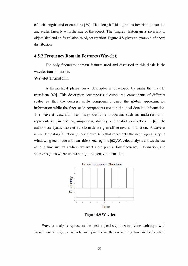
4.5.2 Frequency Domain Features (Wavelet)

The only frequency domain features used and discussed in this thesis is the

wavelet transformation.

Wavelet Transform

A hierarchical planar curve descriptor is developed by using the wavelet

transform [60]. This descriptor decomposes a curve into components of different

scales so that the coarsest scale components carry the global approximation

information while the finer scale components contain the local detailed information.

The wavelet descriptor has many desirable properties such as multi-resolution

representation, invariance, uniqueness, stability, and spatial localization. In [61] the

authors use dyadic wavelet transform deriving an affine invariant function. A wavelet

is an elementary function (check figure 4.9) that represents the next logical step: a

windowing technique with variable-sized regions [62].Wavelet analysis allows the use

of long time intervals where we want more precise low frequency information, and

shorter regions where we want high frequency information

Wavelet analysis represents the next logical step: a windowing technique with

variable-sized regions. Wavelet analysis allows the use of long time intervals where

Figure 4.9 Wavelet

32

we want more precise low frequency information, and shorter regions where we want

high frequency information.

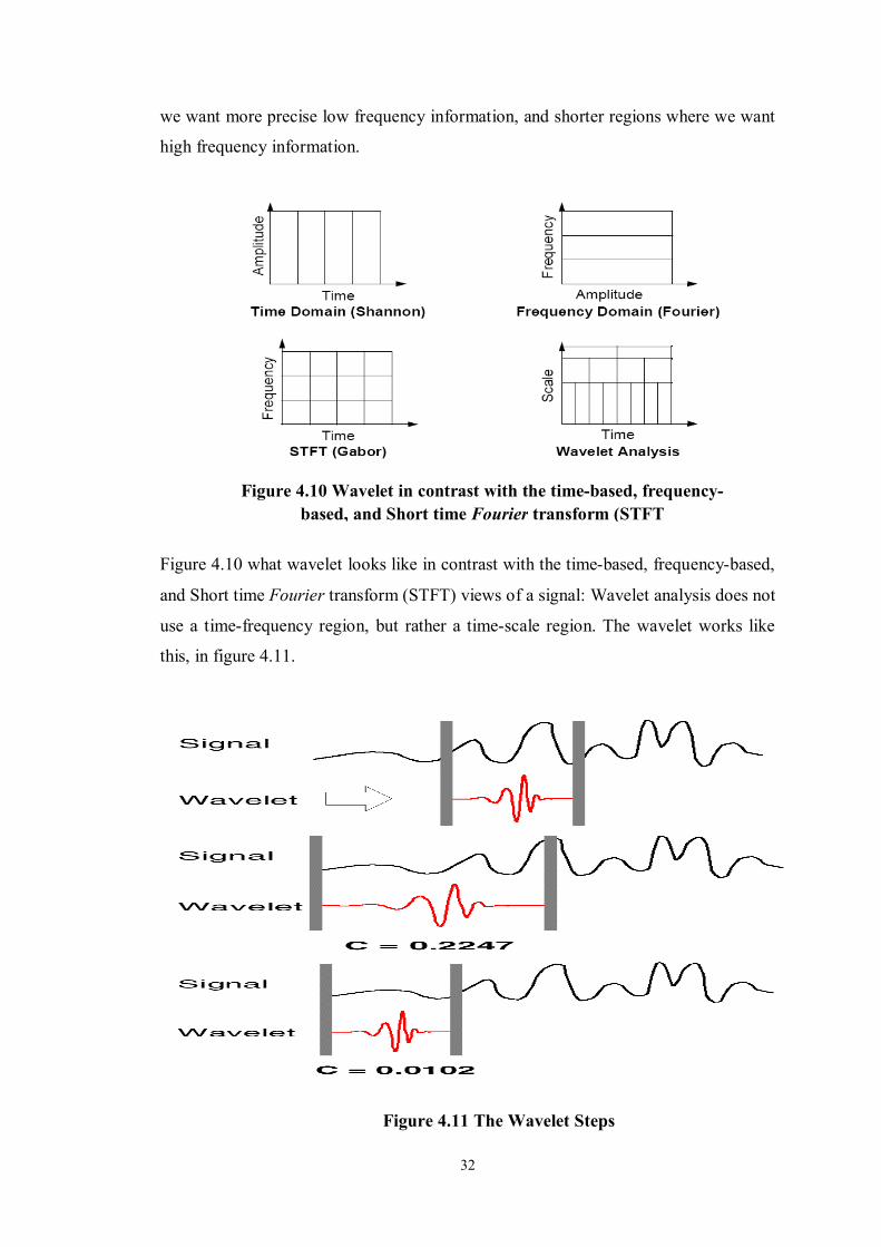
Figure 4.10 what wavelet looks like in contrast with the time-based, frequency-based,

and Short time Fourier transform (STFT) views of a signal: Wavelet analysis does not

use a time-frequency region, but rather a time-scale region. The wavelet works like

this, in figure 4.11.

Figure 4.11 The Wavelet Steps

Figure 4.10 Wavelet in contrast with the time-based, frequency-based, and Short time Fourier transform (STFT

33

The wavelet done in the following steps (check figure 4.11):

1. Take a wavelet and compare it to a section at the start of the original signal.

2. Calculate a correlation coefficient c

3. Shift the wavelet to the right and repeat steps 1 and 2 until the whole signal

covered.

4. Scale (stretch) the wavelet and repeat steps 1 through 3.

5. Repeat steps 1 through 4 for all scales.

The result from this operation is two types of coefficients see figure 4.12, details and

approximation. The detailed coefficients (high frequency) the needed for this thesis.

4.6 Features Enhancement and Manipulations

Not all the extracted features can be helpful in the classification phase

sometimes even these features need to be enhanced and may be the shapes itself need

to be enhanced before the feature extraction phase began. To enhance the dissimilarity

and the differences between the shapes. The features in hand not at equal lengths we

used interpolation and histogram to fix this problem.

Figure 4.12 Wavelet divides the signal into details and approximation.

34

4.6.1 Interpolation

Interpolation is at the heart of various medical imaging applications [63-65].

In volumetric imaging, it is often used to compensate for nonhomogeneous data

sampling. This rescaling operation is desirable to build isometric volumes [66-68].

Another application of this transform arises in the three-dimensional (3-D)

reconstruction of icosahedral viruses [69]. In volume rendering, it is common to apply

by interpolation a texture to the facets that compose the rendered object [70]. In

addition, volume rendering may also require the computation of gradients, which is

best done by taking the interpolation model into account [71]. The essence of

interpolation is to represent an arbitrary continuously defined function as a discrete

sum of weighted and shifted basis functions. An important issue is the adequate

choice of those basis functions. The traditional view asks that they satisfy the

interpolation property, and many researchers have put a significant effort in

optimizing them under this specific constraint [72-77]. Over the years, these efforts

have shown more and more diminishing returns. There is traditional interpolation and

there is generalized interpolation lets discuss both

Traditional Interpolation:

Let us express an interpolated value 푓(휒)at some (perhaps non-integer)

coordinate x in a space of dimension q as a linear combination of samples evaluated at

integer coordinates 푘 = (푘 , 푘 , … . , 푘 )휖푧

풇(흌) = ∑ 풇풌흋풊풏풕(풙 − 풌)∀흌 = 흒ퟏ, 흒ퟐ, 흒ퟑ,… , 흒풒 흐ℝ풒풌흐풛풒 4.18

The sample weights are given by the values of the function휑푖푛푡 푥−푘 . To

satisfy the requirement of exact interpolation, we ask that the function

휑 vanishes for all integer arguments except at the origin, where it must take a

unit value. A classical example of the basis function 휑 is the sinc function, in

which case all synthesized functions are band limited.

Generalized Interpolation

As an alternative approach, let us consider the form

35

풇(흌) = ∑ 풄풌흋(풙 − 풌)∀흌흐ℝ풒풌흐풛풒 4.19

The crucial difference between the classical formulation (1) and the generalized

formulation (2) is the introduction of coefficients 푐 in place of the sample values푓 .

This offers new possibilities, in the sense that interpolation can now be carried in two

separate steps. Firstly, the determination of coefficients 푐 from the samples푓 , then

secondly, the determination of desired values f(x) from the coefficients푐 . The

benefit of this Separation is to allow for an extended choice of basic functions, some

with better properties than those available in the restricted classical case where

푐 = 푓 . The apparent drawback is the need for an additional step. We will see later

that this drawback is largely compensated by the gain in quality resulting from the

larger selection of basic functions to choose from. Some types of interpolation method

are discussed in [78- 80].

1- Nearest Neighbor

The simplest interpolation form a computational standpoint is the nearest

neighbor, where each interpolated output pixel is assigned the value of the nearest

sample point in the input image. This technique is also known as point shift algorithm

and pixel replication. The interpolation kernel for the nearest neighbor algorithm is

defined as:

풉(풙) = ퟏퟎ ≤ |풙| < 0.5ퟎퟎ. ퟓ ≤ |풙|

� 4.20

The frequency response of the nearest neighbor kernel is :

푯(흎) = 풔풊풏풄(흎ퟐ) 4.21

The kernel and its Fourier transform are shown in Figure 4.13.

36

Convolution in the spatial domain with the rectangle function h is equivalent in

the frequency domain to multiplication with a sinc function see figure 4.13. Due to the

prominent side lobes and infinite extent a sinc function makes a poor low-pass filter.

This technique achieves magnification by pixel replication, and magnification by

sparse point sampling for large-scale changes.

2- Linear Interpolation

Linear interpolation is a first degree method that passes a straight line through

every two consecutive points of the input signal see figure 4.14. In the spatial domain,

linear interpolation is equivalent to convolving the sampled input with the following

kernel.

풉(풙) = ퟏ − |풙|ퟎ ≤ |풙| < 1ퟎퟏ ≤ |풙|

� 4.22

푯(흎) = 풔풊풏풄ퟐ(흎ퟐ) 4.23

The kernel is also called triangle filter, roof function or Bartlett window. As shown in

Figure 4.14 the frequency response of the linear interpolation kernel is superior to that

of the Nears neighbor interpolation function, the side lobes are less prominent, so the

performance is improved in the stop band. A pass band is moderately attenuated,

resulting in image smoothing.

|퐻(푥)| h (x)

Figure 4.13 Nearest Neighbor Kernel

37

Linear interpolation produces reasonably good results at moderate cost. But

for even better performance, more complicated algorithms are needed.

풉(풙) =(풂 + ퟐ)|풙|ퟑ − (풂 + ퟑ)|풙|ퟐ + ퟏퟎ ≤ |풙| < 1풂|풙|ퟑ − ퟓ풂|풙|ퟐ + ퟖ풂|풙| − ퟒ풂ퟎ ≤ |풙| < 2

ퟎퟐ ≤ |풙|� 4.24

3- Cubic Interpolation

Cubic interpolation (figure 4.15) is a third degree interpolation algorithm that

fairly well approximates the theoretically optimum sinc interpolation function. The

kernel is composed of piecewise cubic polynomials defined on subintervals (-2,-1), (-

1,0), (0,1) and (1,2). Outside this interval the interpolation kernel is zero. For deriving

the cubic convolution kernel, we have to solve 8 linear equations with 7 unknown

parameters, so the system has one "free" parameter that may be controlled by the user.

The kernel is of form:

The frequency response is:

푹(흎) = ퟏퟐ흎ퟐ 풔풊풏풄ퟐ 흎

ퟐ− 풔풊풏풄(흎) + 풂 ퟖ

흎ퟐퟑ풔풊풏풄ퟐ(흎) − ퟐ풔풊풏풄(흎) − 풔풊풏풄(ퟐ흎) 4.25

|퐻(푓)| h (x)

Figure 4.14 Linear Interpolations.

38

Choices for a are a=1. a=0.75 and a=0.5. The performance of the interpolation kernel

depends on a, and the frequency content of the signal. For different signals, different

values of the parameter a gives the best performance.

4- Piecewise Cubic Hermite (PCHIP) Interpolation

For a given np points, interpolation both the function and its derivative with a

cubic polynomial on each subinterval. This approach is called piecewise cubic

Hermite interpolation.

5- B-splines

A B-spline of the degree nd is derived through nd convolutions of the box filter,

Thus, 퐵 =퐵 ∗ 퐵 denotes a B-spline of degree 1. Yielding the familiar triangle

filter. (letter B may stand for basic or basis ). The B-spline of dgree 1 is equivalent to

the linear interpolation. The second degree B-spline 퐵 is produced by convolving

퐵 ∗ 퐵 .

The cubic B-spline B is generated from convolvingB ∗ B . That is B = B ∗ B ∗

B ∗ B . Figure 4.16 summarize the shapes of these low-order B-splines. The cubic

B-spline interpolation kernel is defined as:

풉(풙) = ퟏퟔ

ퟑ|풙|ퟑ − ퟔ|풙|ퟐ + ퟒퟎ ≤ |풙| < 1−|풙|ퟑ + ퟔ|풙|ퟐ − ퟏퟐ|풙| + ퟖퟏ ≤ |풙| < 2

ퟎퟐ ≤ |풙|� 4.26

|퐻(푓)| h (x)

Figure 4.15 Cubic Interploation.

39

Unlike cubic convolution, the cubic B-spline kernel is not interpolatory since

it does not satisfy the necessary constraint that h(0)=1 and h(1)=h(2)=0. Instead, it is

an approximating function that passes near the points but not necessarily through

them. This is due to the fact that the kernel is strictly positive application. When using

kernals with negative lobes, it is possible to generate negative values while

interpolating positive data,. Since negative intensity values are meaningless for

display, it is desirable to use strictly positive interpolation kernels to guarantee the

passivity of the interpolated image.

4.6.2 Image Rotation

To guarantee rotation invariance, it is necessary to convert an arbitrarily

oriented shape into a unique common orientation. First, find the major axis of the

shape. The major axis is the straight line segment joining the two points P1 and P2 on

the boundary farthest away from each other. Then we rotate the shape so that its major

axis is parallel to the x-axis. This orientation is still not unique as there are two

possibilities: P1 can be on the left or on the right. This problem is solved by

computing the centroid of the polygon and making sure that the centroid is below the

major axis, thus guaranteeing a unique orientation. So knowing the coordination of

the shapes points how we can rotate these points? The answer is by using Matrix

rotation.

Figure 4.16 B-spline Interpolation.

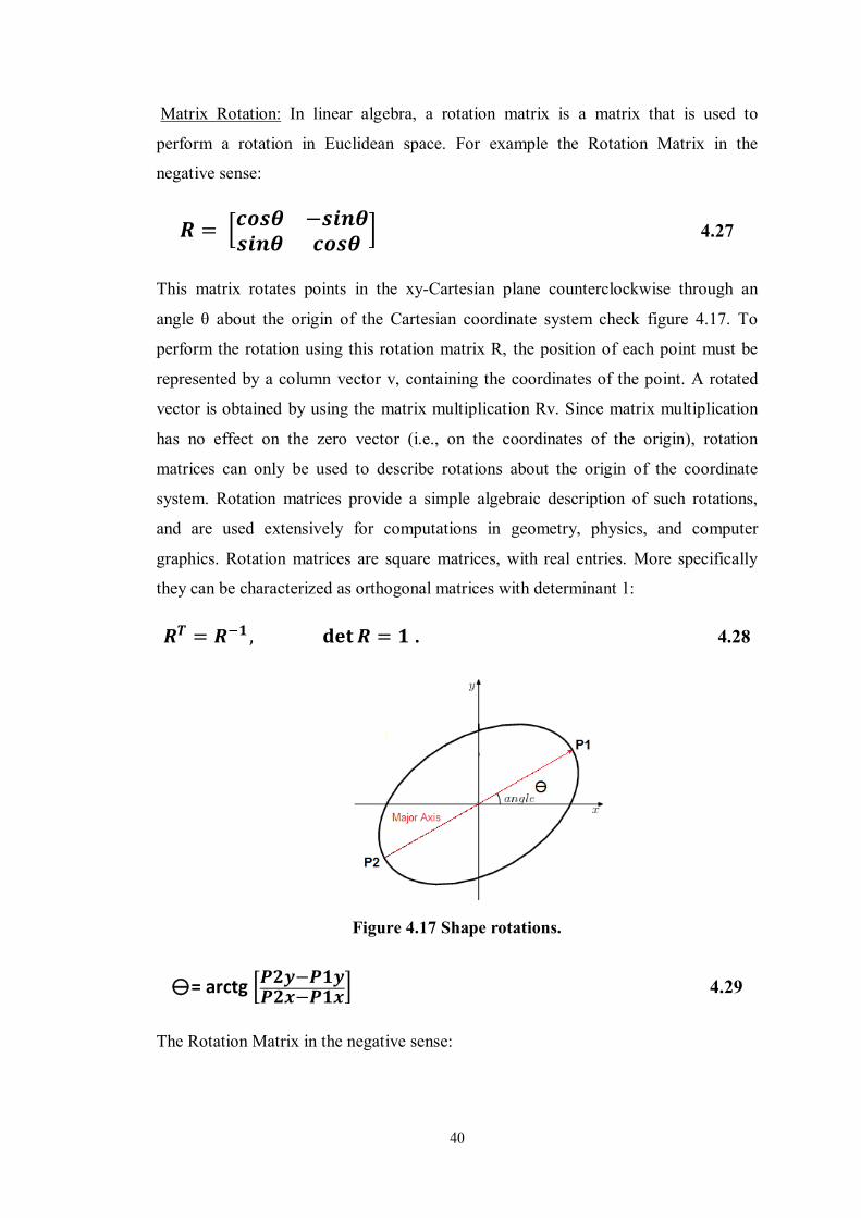
40

Matrix Rotation: In linear algebra, a rotation matrix is a matrix that is used to

perform a rotation in Euclidean space. For example the Rotation Matrix in the

negative sense:

푹 = 풄풐풔휽 −풔풊풏휽풔풊풏휽 풄풐풔휽 4.27

This matrix rotates points in the xy-Cartesian plane counterclockwise through an

angle θ about the origin of the Cartesian coordinate system check figure 4.17. To

perform the rotation using this rotation matrix R, the position of each point must be

represented by a column vector v, containing the coordinates of the point. A rotated

vector is obtained by using the matrix multiplication Rv. Since matrix multiplication

has no effect on the zero vector (i.e., on the coordinates of the origin), rotation

matrices can only be used to describe rotations about the origin of the coordinate

system. Rotation matrices provide a simple algebraic description of such rotations,

and are used extensively for computations in geometry, physics, and computer

graphics. Rotation matrices are square matrices, with real entries. More specifically

they can be characterized as orthogonal matrices with determinant 1:

푹푻 = 푹 ퟏ ,퐝퐞퐭 푹 = ퟏ . 4.28

= arctg 푷ퟐ풚−푷ퟏ풚푷ퟐ풙−푷ퟏ풙 4.29

The Rotation Matrix in the negative sense:

Figure 4.17 Shape rotations.

41

푅 = 푐표푠휃 −푠푖푛휃푠푖푛휃 푐표푠휃 4.30

4.7 Classification/Clustering Techniques

Pattern recognition can also be seen as a classification process. Its ultimate goal is

to optimally extract patterns based on certain conditions and to separate one class

from the others according to this there is two types of classification, supervised

classification and unsupervised classification. With supervised classification [81], we

identify examples of the Information classes (i.e., land cover type) of interest in the

image. These are called "training sites". The image processing software system is

then used to develop a statistical characterization of the reflectance for each

information class. Unsupervised classification [81] is a method which examines a

large number of unknown pixels and divides it into a number of classed based on

natural groupings present in the image values. Unlike supervised classification,

unsupervised classification does not require analyst-specified training data.

Unsupervised classification commonly called Clustering defined according to [82] is a

method of creating groups of objects, or clusters, in such a way that objects in one

cluster are very similar and objects in different clusters are quite distinct. Example of

clustering technique K-Means discussed later.

4.7.1 K-Means

The k-Means algorithm [82] can be divided into two phases: the initialization phase

and the iteration phase. In the initialization phase, the algorithm randomly assigns the

cases into k clusters. In the iteration phase, the algorithm computes the distance

between each case and each cluster and assigns the case to the nearest cluster. The K-

Means algorithm, first developed four decades ago [83], is one of the most popular

centre-based algorithms that attempts to find K clusters which minimize the mean

squared quantization error , MSQE. The algorithm tries to locate K prototypes

(centroids) throughout a data set in such a way that the K prototypes in some way best

represent the data. We can summarize [84] the K-Means algorithm through the

following steps:

42

Algorithm 4.1: K-Means algorithm

Purpose: clustering data sets into K categories.

Input: matrix of features, each row represents features of cell.

Output: K centroids of the K clusters.

Procedure:

1. Initialization

Step1: Define the number of prototypes (K).

Step2: Designate a prototype (a vector quantity that is of the same dimensionality as

the data) for each cluster.

Step3: Assign each data point to the closest prototype. That data point is now a

member of the class identified by that prototype.

Step4: Calculate the new position for each prototype (by calculating the mean of all

the members of that class).

Step5: Observe the new prototypes' positions. If these values have not significantly

changed over a certain number of iterations, exit the algorithm. If they have, go back

to Step 2.

4.7.2 Genetic Algorithm (GA)

Interestingly Genetic algorithms used in both classification types supervised

[85] and unsupervised [86- 90]. GA is considered the heart of this thesis and small

comparison of GA and K-means is accomplished during it.

Genetic algorithms are a stochastic search algorithm, which uses probability to guide

the search. It was first suggested by John Halland [91]; in the seventies. Over the last

twenty years, it has been used to solve a wide range of search, optimization, and

machine learning. Genetic algorithms are a class of parallel adaptive search

algorithms based on the mechanics of natural selection and natural genetic system. It

can find the near global optimal solution in a large solution space quickly. It has been

used extensively in many application areas, such as image processing, pattern

43

recognition, feature selection, and machine learning [92]. It is a powerful search

technique that mimics natural selection and genetic operators. Its power comes from

its ability to combine good pieces from different solutions and assemble them into a

single super solution [93].Genetic algorithms are initial population of solution called

individuals is (randomly) generated, the solutions are evaluated. The algorithm creates

new generations of population by genetic operations, such as reproduction, crossover

and mutation. The next generation consists of the possible survivors (i.e. the best

individuals of the previous generation) and of the new individuals obtained from the

previous population by the genetic operations. The best source of information about

Gas is Holland's adaptation in natural and artificial systems; Holland uses terms

borrowed from mendelian genetics to describe the process: each position in the string

is called a gene. The possible values of each gene are called alleles. A particular string

is called a genotype. The population of strings also called the gene pool. The

organism or behavior pattern specified by a genotype is called a phenotype. If the

organism represented is a function with one or more inputs [94] these inputs are called

detectors. The algorithm of simple GAs in [95-96]. The following steps show how

GA works:

Algorithm 4.2: Genetic algorithm

Purpose: clustering data sets into K categories.

Input: matrix of features, each row represents features of cell.

Output: K centroids of the K clusters.

Procedure:

Step1: Initialization: Generate random population.

Step2: Evaluate the fitness f(x) of each element x in the population.

Step3: The best K elements in the population according to f(x) are the K centroid of

the clusters.

Step4: Create a new population by repeating following steps until the new population

is complete

44

Select two parent from a population according to their fitness (the better

fitness, the bigger chance to be selected)

With a crossover probability cross over the parents to form a new offspring

(children). If no crossover was performed, offspring is an exact copy of

parents.

With a mutation probability mutate new offspring at each element in the

population.

Place new offspring in a new population

Step5: Use new generated population for a further run of algorithm

Step6: If the end condition is satisfied, stop, and return the best solution in current

population. Otherwise go to step 3.

Step 3 needs further explanation, for the K best elements each of them considered

centroids for K clusters. Each vector in the data set in hand measures the distance

between it and the K centroids. The smallest distance to a centroid gives indication

that this vector belongs to that cluster with that centroid. According to this the

evaluation of fitness function accomplished.

GA parameters:

A. Population

A population consists of n individuals where N is chosen by the designer of the GA's

[97]. Every individual has a chromosome which consists of Lg genes. The

chromosome is often referred to as the genotype of an individual.

B. Initialization

Initialization means initialize the genes of all individuals randomly or with

predefined values it's up to the GA designer. These individuals are the starting points

in the search space for the simple GA.

C. Evaluation

Calculate the fitness of each individual by decoding each chromosome and

applying the fitness function to each decode individuals. The decoding creates a

phenotype based on a genotype.

45

D. Scaling Function

Scaling function specifies the function that performs the scaling [98]. The options

are:

Rank — scales the raw scores based on the rank of each individual instead of its

score. The rank of an individual is its position in the sorted scores. An individual

with rank r has scaled score proportional to √

. So the scaled score of the most fit

individual is proportional to 1, the scaled score of the next most fit is proportional

to √

, and so on. Rank fitness scaling removes the effect of the spread of the raw

scores. The square root makes poorly ranked individuals more nearly equal in

score, compared to rank scoring.

Proportional — Proportional scaling makes the scaled value of an individual

proportional to its raw fitness score.

Top— Top scaling scales the top individuals equally. Selecting Top displays an

additional field, Quantity variable, which specifies the number of individuals that

are assigned positive scaled values. Quantity can be an integer between 1 and the

population size or a fraction between 0 and 1 specifying a fraction of the population

size. The default value is 0.4. Each of the individuals that produce offspring is

assigned an equal scaled value, while the rest are assigned the value 0.

Shift linear — Shift linear scaling scales the raw scores so that the expectation of

the fittest individual is equal to a constant multiplied by the average score.

E. Selection

Select specific individuals from the population to be the parents that will used to

create new individuals there is many methods are used to choose those parents [97].

The selection method specifies how the genetic algorithm chooses parents for the next

generation. The methods are:

Stochastic uniform —Stochastic uniform, lays out a line in which each parent

corresponds to a section of the line of length proportional to its scaled value. The

algorithm moves along the line in steps of equal size. At each step, the algorithm

allocates a parent from the section it lands on. The first step is a uniform random

number less than the step size.

46

Remainder — Remainder selection assigns parents deterministically from the

integer part of each individual's scaled value and then uses roulette selection on the

remaining fractional part. For example, if the scaled value of an individual is 2.3,

that individual is listed twice as a parent because the integer part is 2. After parents

have been assigned according to the integer parts of the scaled values, the rest of

the parents are chosen stochastically. The probability that a parent is chosen in this

step is proportional to the fractional part of its scaled value.

Uniform — Uniform selection chooses parents using the expectations and number

of parents. Uniform selection is useful for debugging and testing, but is not a very

effective search strategy.

Roulette — Roulette selection chooses parents by simulating a roulette wheel, in

which the area of the section of the wheel corresponding to an individual is

proportional to the individual's expectation. The algorithm uses a random number

to select one of the sections with a probability equal to its area.

Tournament — Tournament selection chooses each parent by

choosing Tournament size players at random and then choosing the best

individual out of that set to be a parent. Tournament size must be at least 2.

E. Recombination

Individuals from the set selected-parents are mated at random and each pair

created offspring using 1 point crossover or 2-point crossover.

47

F. Mutation

Mutation is a random change of one or more genes [97] Every chromosome is

simply scanned gene by gene and with a mutation rate Pm a gene is

changed/swapped, i.e. 0 1 and 1 0 the probability for a mutation is usually kept small,

i.e. Pm = 1/Lg such that we can expect one mutated gene per chromosome.

G. Stop Criterion

Stopping criteria is when the GA should stop. A simple and easy to implement

stopping criterion is to stop the simple GAs if no improvement of the best solution has

been made for a (large) predefined number of generations, where one generation is

one turn through the do-until loop in algorithm in Figure, there are other different

stopping criteria: first limited number of generations, limited consumed time during

the process. In the next chapters we discuss the practical work of thesis, in other

words we apply basic mention theories in this chapter in the next following chapters

Figure 4.18 Recombination

48

Chapter 5: The Proposed System

5.1 Introduction In this thesis the proposed system consist of four stages check figure 5.1. These

stages are: data collection phase, pre-processing phase, feature extraction phase and

finally classification phase.

Figure 5.1 The Proposed System.

5.2 Data Collection Stage In this stage several types of equipments used. First we need equipments and tools to

draw bloods and make a blood films from these samples. Second we need equipments

and tools for blood films images capturing under the microscope.

Data Collection Stage

Pre-processingStage

FeaturesExtraction Stage

ClassificationStage

Figure 5.2 The Equipments (a)In the left the equipment needed for blood drawing and blood films making, (b) In the right the needed equipments for blood films

image capturing under the microscope.

49

In the left of figure 5.2 the equipment needed for blood drawing and blood films

making these equipments in details discussed in table 5.1. The equipment needed and

used in this thesis are:

Table 5.1 Blood drawing and Making Equipments

Amount Items 100 Needles 100 Sernges 100 Tubes 2 White Cotton 3 bottles each 125 ml Stains (right stain) 100 Blood Slides 100 Blood Slides cover

These equipments from Needles to Cotton used to draw human blood (sick and

healthy people) while the rest are used to make the blood films which is discussed

more thoroughly in Appendix B.

In the right of figure 5.2 are the equipment used in the blood films image capturing

under the microscope, in table 5.2 discussed in details:

Table 5.2 Blood films images capturing under the microscope Equipments and tools. Items Description Amount Video Wireless Camera Receiver USB 2.0 Video Adapter with Audio 1 Electronic Eyepiece Model: coomo20N 1

Table 5.2 these are the actual tools that used in this thesis where the video camera

gives a video stream to what is available under the microscope which is in our case

blood films. While the video card is just an adapter so we can connect the video

camera to our laptop directly and then we can take images as much as we can. There

are an alternative tool can be used here which is a C-mount adapter check figure 5.3

with any kind of camera. In such case the type of C-mount adapter depends very

much on the camera and the microscope types. But in our case the video camera we

use works very good with any type of microscope. This is what makes it's more

appealing.

50

The number of obtained samples are hundred (100), for 100 different persons,

meaning 100 pictures, these images has 114 shapes for Burr cells, 128 shapes for

Normal cells, 59 shapes for Teardrop cells and 118 shapes for Sickle cells.

In the classification phase we classify data to different categories, once into

four categories (normal cells, sickle cells, teardrop cells and burr cells), where the last

three categories are abnormal cases; second into two categories: normal and

abnormal. Example of captures blood films image in figure 5.4. The software we used

for such process is Matlab Software where it has Genetic Algorithm and K-Means functions.

5.3 Preprocessing Stage

First we need to split the blood cells from the background. This step is achieved first

by using Hough transforms, the resultant image shown in figure 5.5.

Figure 5.4 Sample of the blood films images in hand.

Figure 5.3 C-Mount Adapter.

51

As you may notice, sometimes Hough transformer ignores cells or imagines

the existence of cells and fails miserably in case of overlapping cells and ignores

abnormal cells. Another approach is to use color based segmentation to separate red

blood cells from other cells and from the background in a single step. K-means used

to cluster the blood films images into 3 cluster, first cluster is red blood cells, second

cluster is the background and third cluster is for other cells, repeating clustering three

times to avoid local minima. The result from clustering the blood films images in

RGB space; each color represents different cluster alone, nuclei of cells and the

background in one cluster not quite the wanted result. Each colors in figure 5.6 (a)

represents a different cluster.

The features chosen to be fed into K-means (8 features) are:

R: red value for each pixel. B: blue value for each pixel.

G: green value for each pixel. x: x- coordinate for each pixels.

Figure 5.6.Clustering using K-means in RGB space, Figure 5.3 (a) the clustering

result, Figure 5.3 (b) the original image.

Each color Represents different cluster

100 200 300 400

The Original Image

100 200 300 400

50

100

150

200

250

50

100

150

200

250

Figure 5.5 Same image with Hough Transformer for cells detections.

52

y: y- coordinate for each pixels I: intensity value for each pixel.

S: saturation value for each pixel. H: hue value for each pixel.

Using these equations:

퐈 = ퟏퟑ(퐑 + 퐆 + 퐁) 5.1

퐒 = ퟏ − ퟑ(퐑 퐆 퐁)

× 퐚 , Where a is the minimum of R, G and B

퐇 = 퐜퐨퐬 ퟏ( ퟎ.ퟓ×((퐑 퐆) (퐑 퐁))((퐑 퐆)ퟐ (퐑 퐁)×(퐆 퐁)ퟎ.ퟓ)

) 5.2

Using same clustering techniques (K-Means) and the same features for

segmenting/clustering but in the LAB space, each cluster in a separate image alone is

shown in figure 5.7.

In figure 5.7, the white cells (large cells) still segmented with the red blood cells, this

means that more following steps required; the result form the clustering in the RGB

space is much better, since colors manipulation operation are more flexible. In

segmenting (clustering) in the LAB space the image entirely fed into K-Means; only

pink cells must be in one cluster along with their centers (nuclei).

Figure 5.7.Clustering of foreground and using K-means in LAB space.

objects in cluster 2objects in cluster 1

53

After segmenting/clustering the blood films images using K-means into 3 clusters,

first cluster is Pink objects (red blood cells), second cluster is the background and

third cluster is for the other cells all that in RGB space, repeating the clustering

process three times to avoid local minima. Converting figure 5.8 into binary image is

presented in figure 5.9.

For binary image, some morphological operations performed to clean the image from

unwanted parts (such as the fractions of white cells). First: opening operation with

disk of five pixels radius is done (notice here that the images of the blood films are of

the same size).

Figure 5.9. Binary image of figure 5.8

Figure 5.8 Third cluster red cells.

objects in cluster 3

54

The morphological operations that used in figure 5.10 are necessary to separate the

red blood cells alone, these red blood cells is cleaned and ready to be used. Now, the

next problem that we faced is the overlapped cells, so the next step is clustering (or

separating) the overlapped cells from the non-overlapped cells. The K-Means

clustering technique is used also for such purpose:

The suggested features to be fed to the K-means to accomplish such task are:

- The object size (number of pixels in each object).

- The maximum distance between any two pixels (Euclidean distance used).

푬풅(퐄퐮퐜퐥퐢퐝퐢퐚퐧퐝퐢퐬퐭퐚퐧퐜퐞) = (풙ퟏ − 풙ퟐ)ퟎ.ퟓ + (풚ퟏ − 풚ퟐ)ퟎ.ퟓ 5.3

Applying equation 5.3 on the final resultant image, after the morphological operations

(figure 5.10-d), we have two clusters, shown in figure 5.11, one for overlapped cells

and the other for non-overlapped cells, but the results not very stable meaning that it

may give different result from run to run.

Figure 5.10 Some morphological operations: (a) Binary image after opening morphological operation (R=5 pixels). (b) Image filling morphological operation (holes). (c) Opening morphological operation (R=2 pixels). (d) Closing morphological operation

55

To solve this critical problem, another feature must be included in order to separate

both groups more exclusively. So new feature added to the previous set of features

which is:

-The maximum distance between the median point (centroid point of the object) and

any other pixel in the object (Euclidian distance used).

Be aware that each shape (object) is resized to fix size before the previous features are

taken and before clustering operation is done. The result from such modification

produces stable result after executing the code at any number of times, i.e. the

stability is achieved, as shown in figure 5.12, no matter how many times the code is

run or whatever the blood film (abnormal or normal cases) the result is the same. The

success rate for such clustering was 100%.

The number of cells in a particular area is important feature for doctors and

hematologists. So for counting the objects (cells) in image correctly, the overlapped

cells should be separated into the actual number of cells that overlapped. Ordinary

Figure.5.12 The final result from clustering overlapped / non-overlapped cells.

Figure 5.11 Two cases for clustering of overlapped/non-overlapped cells. (a) is good

results. (b) is bad results.

56

counting will count the overlapped cells as one object. So we apply the watershed

morphological operation at overlapped cells to segment it to the approximate number

of cells that overlapped. Figure 5.13 show the overlapped cells in part (a), while part

(b) separate each cell from the overlapped cells. This is done by first applying

distance transformer to the objects then on the result applying the watershed, which

gave good result.

By zooming in for one overlapped cells object, figure 5.14, we will find that there are

several segmentation lines in between the two overlapped cells, which indicate

improper segmentation. The solution for such problem is to enhance (or more

accurate filter) the image in the grey level before converting it to binary image in the

first place.

The image filtered using smoothing edge filter then watershed applied which is give

much better result as illustrated in figure 5.15.

Figure 5.14 Two Overlapped cells.

Figure 5.13. Watershed morphological operation: (a) overlapped cells. (b) Segmented overlapped cells using watershed.

57

Previous phase results gave each red blood cell alone as required to count the

number of cells, but the produced binary image lost a lot of it is properties due to

enhancement and morphological operations usage. To solve this problem, we located

the centroid for each object in the binary image in hand and convert the original

image (the first blood films images) to binary image, and use the centroids as flags

to locate the wanted objects as shown in figure 5.16.

Getting the red blood cells alone then getting these cells from the original image with

all their details intact, clustering the overlapped and non-overlapped cells and

removing the boundary object, with all that done the preprocessing phase is finished.

This can be summaries in the following steps:

1- Resize images to one size (Average size among image sizes).

2- Clustering the image based on color. (Features were: red, green, blue, the

coordination, saturation, intensity and hue), we are only concerned with the

pink objects (the red blood cells).

3- Filtering the pink cluster with smoothing filter then convert it into binary

image.

4- Applying opening morphological operation (R=5 pixels) on the binary image.

Figure 5.16 Cell Segmentation (a) The binary image (non-overlapped cells). (b) The centroids of cells in binary image as flag in the original binary image. (c) The resultant

image after flagging operation

Figure 5.15 Overlapped cells after smoothing filter

58

5- Applying image filling morphological operation (holes) on the result from the

third step.

6- Applying opening morphological operation (R=2 pixels) on the result from the

fifth step.

7- Applying closing morphological operation (holes) on the result from the sixth

step.

8- Clustering the result from sixth step based on these features:

- The object size (no of pixels in each object).

- The maximum distance between any two pixels (Euclidean distance).

- The maximum distance between the median point (object centroid) and any

other pixel in the object (Euclidian distance).

This is step done in order to get the overlapped cells alone and non-overlapped cells

(worked as intended).

9- Applying watershed morphological operation on the cluster that contains non

overlapped cells.

10- The object exist in result of sixth step is the only object we concerned in, but

they lose their distinguishing, so the centroids of each object in the binary

image from the sixth step made as flags to the binary image of the original

image, mapping the original image by centroids (flags) to locate object

needed with all their details.

5.4 Feature Extraction Stage After the isolation of the red blood cells from the image, and clustering the

overlapped cells away from the non-overlapped cells, the feature extraction phase is

come next, to extract the unique features of the individual cells which distinct each

cell. The suggested methodology in this phase is to extract the features in time domain

and frequency domain. Figure 5.17 demonstrates the methods that been used to

extract the features which needed to be fed into the classifier and their relationships.

59

Figure 5.17 Methods that used to extract features.

5.4.1 Spatial Domain Features

In this thesis, several functions in time domain were been applied to extract

suitable red blood cells features. These features were fed to our classifier to achieve

best results as much as possible. As explained in chapter 4, Centroid Distance

Function (CDF), and Triangular Area Representations (TAR) are used in this phase,

but there are some pre-processing steps should be achieved before extracting the CDF

and TAR features or even frequency domain features for each individual cell. These

steps in time domain are as follows.

1- Bounding rectangle (BR).

This means containing the object (in our case each RBC cell) in a bounding rectangle.

2- Fixing the orientation.

Unifying the orientation angle for all shapes (cells), this is done by using the

following procedures:

1) Measuring the angle between the major axis and the x-axis of the shape (cell)

and called the angle .

2) Multiplying each point’s coordination by R.

Explanation: the shapes (cells) need to have common orientations angle;

orientation angle is the angle between the major axis of shape with the x-axis; So in

order to make all shapes (cells) have a common orientation angle which in our case is

Features

Spatial Domain Features

Shape Signatures

Centroid Distance Features

Triangular Area Representation

Shape Descriptor

Frequency Domain Features Wavelet

60

zero (meaning the major axis lying on the x-axis) we need to know the current

orientation and multiply the current coordination of the shape (cell) pixels to R matrix

that described in equation 5.6.

= arctg 퐏ퟐ퐲−퐏ퟏ퐲퐏ퟐ퐱−퐏ퟏ퐱 5.4

The rotation matrix in the negative sense:

퐑 = 퐜퐨퐬훉 −퐬퐢퐧훉퐬퐢퐧훉 퐜퐨퐬훉 5.5

Where is the angle used to rotate the shapes (cells) in (clock wise or in the negative

sense); in our case is the current orientation angle of the shape (to make the

orientation zero).

3- Resize the cell size to fix size.

Using interpolating which discussed thoroughly in the previous chapter.

4- Rotate the image around the centroid.

To guarantee rotation invariance, it is necessary to convert an arbitrarily oriented

shape (in our case cells) into a unique common orientation. First, find the major axis

of the shape. The major axis is the straight line segment joining the two points 푃 and

푃 on the boundary farthest away from each other. Then we rotate the shape (cell) so

that its major axis is parallel to the x-axis. This orientation is still not unique as there

are two possibilities: 푃 can be on the left or on the right. This problem is solved by

computing the centroid of the polygon (shape or cell) and making sure that the

centroid is below the major axis, thus guaranteeing a unique orientation. Let us now

Figure 5.18. Fixing the orientation. (a) Before Shape rotation. (b) After shape rotation

61

consider scale and translation invariance. We define the bounding rectangle (BR) of a

shape as the rectangle with sides parallel to the x and y axes just large enough to cover

the entire shape (after rotation). Note that the width of the BR is equal to the length

of the major axis. To achieve scale invariance, we proportionally scale all shapes so

that their BRs have the same fixed width (pixels). Since major axis of the shape laying

on the x-axis (after fixing the orientation) the shape will looks like figure 5.18 (b).

So 풴 = 풴 and length of the major axis is 풳 −풳

After finding the centroid of the shape (풳,풴) ; if 풴 > 풴 or if 풴 > 풴 then the

centroid is above the major axis else the centroid below the major axis. In the graph,

the 풴 is below the major axis, an example is presented in figure 5.19

Each shape with its CDF values and TAR representations values the lengths

of each representatives features is variant than others and all that discussed

significantly obvious in the data description tables.

SD (Shape Descriptor):

Features = [Solidity, E, Circle Ratio, Rectangularity, Convexity, Ellipse Ratio, Extent,

Ecc, R1, R2];

7- Solidity: Scalar specifying the proportion of the pixels in the convex hull that are

also in the region. As stated in chapter 4 computed using the equation 4.6.

8- Eccentricity (E): Scalar that specifies the eccentricity of the ellipse that has the

same second-moments as the region. The eccentricity is the ratio of the distance

between the foci of the ellipse and its major axis length. The value is between 0

and 1. (0 and 1 are degenerate cases; an ellipse whose eccentricity is 0 is actually a

circle, while an ellipse whose eccentricity is 1 is a line segment.) .Eccentricity’s

(a) (b)

Figure 5.19 Shape rotation for: (a) RBC Sickle. (b) RBC Teardrop.

Binary

Fix Orientation

Binary

62

the measure of aspect ratio. It is the ratio of the length of major axis to the length

of minor axis.

9- Circularity ratio represents how much a shape is similar to a circle. Circularity

ratio is the ratio of the area of a shape to the area of a circle having the same

perimeter. Check chapter 4 for equations 4.7 to 4.12.

10- Rectangularity: the Area of the shape divided by the area of the minimum

bounding box. Rectangularity represents how rectangular a shape is, i.e how much

it fills its minimum bounding rectangle see equation 4.13 in chapter 4.

11- Convexity: is defined as the ratio of perimeters of the convex hull over that of

the original contour, check equation 4.14 in chapter 4.

12- Ellipse Ratio: first with knowing the next two concepts:

A- Major Axis Length: Scalar specifying the length (in pixels) of the major axis

of the ellipse that has the same normalized second central moments as the

region.

B- Minor Axis Length: Scalar; the length (in pixels) of the minor axis of the

ellipse that has the same normalized second central moments as the region.

Where Ellipse Ratio: is ratio of the shape area and the ellipse area with the same

minor axis and major axis of the shape.

7. Extent: Scalar that specifies the ratio of pixels in the region to pixels in the total

bounding box. Computed as the Area of the shape divided by the area of the bounding

box.

8. Ecc: first let's understand the following definition:

Longest Length: is a variable we made to measure the distance between farthest two

points at the boundary.

So, Ecc = 푴풊풏풐풓푨풙풊풔푳풆풏품풕풉푳풐풏품풆풔풕푳풆풏품풕풉

5.6

First we calculate distance of the farthest point on the boundary and the closest point

on the boundary to the centroid.

D1= the longest distance (Centroid to boundary).

D2= the shortest distance (Centroid to boundary).

63

9. R2 is the ratio of longest distance of the boundary to the centroid to the major axis

length of the shape

R1= 푫ퟏ푴풂풋풐풓푨풙풊풔풍풆풏품풕풉

5.7

10. R2 is the ratio of shortest distance of the boundary to the centroid to the major

axis length of the shape

R2= 푫ퟐ푴풂풋풐풓푨풙풊풔풍풆풏품풕풉

5.8

Spatial Domain Features Data sets

After applying all what is mention before we obtained several data sets, each of these

data sets described in a table where the maximum value of the features and the

minimum value of the features also the maximum length of the features and the

minimum length of these features, where in front of each cell type these values

recorded and the number of cells in question. First the CDF:

CDF Data Set Description

Table 5.3 Data Set Description for Centroid Distance Function (CDF) features for each type of cells

Number of Cells

Minimum Features Length

Maximum Features Length

Minimum Features Value

Maximum Features Value

Type of The Cell

114 864 1515 8.4582e-004 1 Burr 118 254 962 0.004 1 Sickle 59 499 1271 0.0048 1 Tear drop 128 990 1540 0.0029 1 Normal

As mention before this table (table 5.3) is a description for the Centroid Distance

Function (CDF) features. These data sets contains features for four different types of

cells the number of cells for each type of cell is variant and the lengths of these

features not equal. For example the first raw is for Burr cells where the maximum

feature value for this type of cells is 1 while the minimum is 8.4582e-004, in the other

hand the maximum feature length for this cell type is 1515 while the minimum feature

length is 864. Other rows (cell types) read in the same manner.

64

TAR Data Sets Description

Table 5.4 Data Set Description for Triangular Area Representation (TAR) features for each type of cells

Number of Cells

Minimum Features Length

Maximum Features Length

Minimum Features Value

Maximum Features Value

Type of The Cell

114 864 1515 -17.5135 1 Burr 118 254 962 -14.4444 1 Sickle 59 499 1271 -43 1 Tear drop 128 990 1540 -9.5172 1 Normal

This table (table 5.4) is a description for the Triangular Area Representation(TAR)

features. This data set contains features for four different types of cells the number of

cells for each type of cell is variant and the lengths of these features not equal. For

example the fourth raw is for Normal cells where the maximum feature value for this

type of cells is 1 while the minimum is -9.5172, in the other hand the maximum

feature length for this cell type is 1540 while the minimum feature length is 990.

Other rows (cell types) read in the same manner.

The following two tables (table 5.5 and table 5.6) are also for TAR features, but here

the TAR parameter ts which discusses in chapter 4 manipulated. Where in the table

5.4 ts have the value 3, while in table 5.5 ts equals half of the number of boundary

points, and in table 5.6 ts equals quarter the number of boundary points.

Table 5.5 Data Set Description for Triangular Area Representation (TAR) features for each type of cells

Number of Cells

Minimum Features Length

Maximum Features Length

Minimum Features Value

Maximum Features Value

Type of The Cell

114 864 1515 -1.4722 1 Burr 118 254 962 -2.7845 1 Sickle 59 499 1271 -2.0551 1 Tear drop 128 990 1540 -1.4419 1 Normal

This table (table 5.5) is a description for the Triangular Area Representation(TAR)

features (ts=1-N/4; N=number of boundary points). This data set contains features for

four different types of cells the number of cells for each type of cell is variant and the

lengths of these features not equal. For example the fourth raw is for Normal cells

where the maximum feature value for this type of cells is 1 while the minimum is -

2.0551, in the other hand the maximum feature length for this cell type is 1540 while

the minimum feature length is 990. Other rows (cell types) read in the same manner.

65

Table 5.6 Data Set Description for Triangular Area Representation (TAR) features for each type of cells

Number of Cells

Minimum Features Length

Maximum Features Length

Minimum Features Value

Maximum Features Value

Type of The Cell

114 864 1515 -1.7321 1 Burr 118 254 962 -2.4783 1 Sickle 59 499 1271 -1.6558 1 Tear drop 128 990 1540 -1.2620 1 Normal

This table (table 5.6) is a description for the Triangular Area Representation (TAR)

features (ts=1-N/2; N=number of boundary points). This data set contains features for

four different types of cells the number of cells for each type of cell is variant and the

lengths of these features not equal. For example the second raw is for Sickle cells

where the maximum feature value for this type of cells is 1 while the minimum is -

1.6558, in the other hand the maximum feature length for this cell type is 1271 while

the minimum feature length is 499. Other rows (cell types) read in the same manner.

SD Data Set Description

Table 5.7 Data Set Description for Shape Descriptor (SD) features for each type of cells

Number of Cells

Minimum Features Length

Maximum Features Length

Minimum Features Value

Maximum Features Value

Type of The Cell

114 12 12 0.1754 0.9912 Burr 118 12 12 0 1 Sickle 59 12 12 0.1485 1 Tear drop 128 12 12 0.1630 1 Normal

This table (table 5.7) is a description for the Shape Description (SD) features this data

set contains features for four different types of cells the number of cells for each type

of cell is variant and the lengths of these features are equal. For example the third raw

is for Teardrop cells where the maximum feature value for this type of cells is 1 while

the minimum is 0.1485, in the other hand the maximum feature length for this cell

type is equal the minimum feature length which is 12. Other rows (cell types) read in

the same manner.

5.4.2 Frequency domain Features (Wavelet Transformation) In this domain, wavelet transform is applied into binary shapes to extract

frequency features, another idea was to apply distance transformer on the binary

shapes (cells) which give more information about the shape then apply wavelet to the

66

result. As discussed in chapter 4 the distance transformer is labeling of each pixel of

the object by the distance to the closest point in the background.

For applying wavelet to the shapes (cells) the wavelet applied till the level three

with Daubechies 6 (db6) check figure 5.20. This signal properties are: asymmetric,

orthogonal, biorthogonal, all that makes it is the perfect one to be used with shapes in

general especially cells. The Obtained results (Data sets) are the detailed coefficients

(high frequency) of this process.

Wavelet Data Sets

Table 5.8 Data Set Description for Wavelet features for each type of cells Number of Cells

Minimum Features Length

Maximum Features Length

Minimum Features Value

Maximum Features Value

Type of The Cell

114 15 15 -3.1039 10.3508 Burr 118 15 15 -3.9622 10.4481 Sickle 59 15 15 -2.6596 10.8553 Tear drop 128 15 15 -3.0436 10.8359 Normal

This table (table 5.8) is a description for the wavelet features this data obtained

from applying the wavelet on the cells in the binary form. The data set contains

features for four different types of cells the number of cells for each type of cell is

variant and the lengths of these features are equal. For example the third raw is for

Teardrop cells where the maximum feature value for this type of cells is 1 while the

minimum is -2.6596, in the other hand the maximum feature length for this cell type is

equal the minimum feature length which is 15. Other rows (cell types) read in the

same manner.

Figure 5.20 The Wavelet Daubechies 6 (db6)

67

Table 5.9 Data Set Description for Wavelet features for each type of cells Number of Cells

Minimum Features Length

Maximum Features Length

Minimum Features Value

Maximum Features Value

Type of The Cell

114 15 15 -10.2216 129.8418 Burr 118 15 15 -12.2198 90.2513 Sickle 59 15 15 -9.8820 128.8718 Tear drop 128 15 15 -11.8421 149.4929 Normal

This table (table 5.9) is a description for the wavelet features this data obtained

from applying the wavelet on the cells in the binary form. The data set contains

features for four different types of cells the number of cells for each type of cell is

variant and the lengths of these features are equal. For example the first raw is for

Burr cells where the maximum feature value for this type of cells is 1 while the

minimum is -10.2216, in the other hand the maximum feature length for this cell type

is equal the minimum feature length which is 15. Other rows (cell types) read in the

same manner.

First: Interpolating

There are five interpolation methods used to do this work, they are: nearest, linear,

spline, cubic, pchip:

Nearest: Nearest-neighbor interpolation; the output pixel is assigned the value of the

pixel that the point falls within. No other pixels are considered.

Linear: linear interpolation; the output pixel value is a weighted average of pixels in

the nearest 2-by-2 neighborhood

Cubic: cubic interpolation; the output pixel value is a weighted average of pixels in

the nearest 4-by-4 neighborhood.

Pchip: applying cubic interpolation on subintervals gives pchip.

68

Second: Histogram

Histogram in figure 5.21 plots the data values to their frequency on the data

(y-axis). That can be done with fixed size where the numbers of data values (sub-

intervals) are fixed in order to unify the size of the features set.

5.5 Classification and Selection Stage

To use a genetic algorithm, we must represent a solution to our problem as a

genome (or chromosome). The genetic algorithm then creates a population of

solutions and applies genetic operators such as mutation and crossover to evolve the

solutions in order to find the best solutions. The most important aspects of using

genetic algorithms are: (1) definition of the objective function, (2) definition and

implementation of the genetic representation, and (3) definition and implementation

of the genetic operators. For the Genetic algorithm which is the heart of this thesis,

GA used in unsupervised learning (Clustering) the data. The objective function

Elements of the population푥 = (푥 , 푦 );

Centroid of the cluster i is (푥 , 푦 )

Centroid of the cluster j is (푥 , 푦 )

푆푖푚 = | | ∑ (푥푥 , 푦푥)푥 −(푥푖, 푦푖) 5.9

Figure 5.21 Histogram of the feature vector into fixed size of bins.

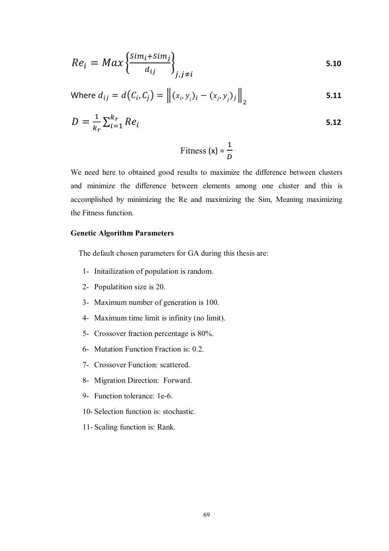
69

푅푒 = 푀푎푥,

5.10

Where 푑 = 푑 퐶 , 퐶 = (푥푖, 푦푖) − (푥푗, 푦푗) 5.11

퐷 = ∑ 푅푒 5.12

Fitness (x) =

We need here to obtained good results to maximize the difference between clusters

and minimize the difference between elements among one cluster and this is

accomplished by minimizing the Re and maximizing the Sim, Meaning maximizing

the Fitness function.

Genetic Algorithm Parameters

The default chosen parameters for GA during this thesis are:

1- Initailization of population is random.

2- Populatition size is 20.

3- Maximum number of generation is 100.

4- Maximum time limit is infinity (no limit).

5- Crossover fraction percentage is 80%.

6- Mutation Function Fraction is: 0.2.

7- Crossover Function: scattered.

8- Migration Direction: Forward.

9- Function tolerance: 1e-6.

10- Selection function is: stochastic.

11- Scaling function is: Rank.

70

Chapter 6: The Proposed System Results

6.1 Introduction

In this chapter the results from the proposed system in chapter 5 is discussed. The

categories are four: normal cells, Sickle cells, Burr cells and Tear drop cells. In other

cases the data (set of features) classified into two categories: normal cells and

abnormal cells. Note that Sickle cells, Burr cells and Teardrop cells considered

abnormal cells. We applied the designed GA with the previous objective function

and with the previous parameters mentioned in last of chapter 5.

6.2 Spatial Domain Results

The results obtained with the spatial domain data sets are discussed in the following

two sections, first CDF and the second TAR:

6.2.1 Centroid Distance Function (CDF) Results

The CDF features have different lengths for different cases and they are not equal

each others, to address these problem two solutions were suggested:

First using interpolation:

Interpolation works by using known data to estimate values at unknown

points. For example: if we wanted to know the temperature at noon, but only

measured it at 10AM and 12:30PM, we could estimate its value by performing a

linear interpolation: In this case two problems presented themselves first we must

choose the length of data as a parameters for the interpolation process (what is the

appropriate length?), second problem there are several types of interpolation methods

(which one is the best in our application?). A suggested solution for these two

problems a study made for three possible lengths (minimum, mean and maximum

length) and for five interpolation methods:

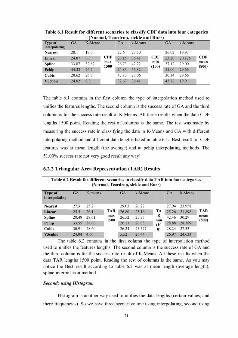
71

Table 6.1 Result for different scenarios to classify CDF data into four categories (Normal, Teardrop, sickle and Burr)

Type of interpolating

GA K-Means GA k-Means GA k-Means

Nearest 20.1 19.0 CDF max 1500

27.6 27.50 CDF min

(100)

26.02 19.97 CDF mean (800)

Linear 24.07 0.8 28.15 36.41 23.20 20.125 Spline 33.87 32.62 26.73 42.72 37.12 29.00 Pchip 44.33 26.7 24.83 36.82 51.00 29.66 Cubic 20.62 26.7 47.87 27.06 30.34 29.66 V5cubic 24.02 0.8 32.67 36.41 43.78 19.9

The table 6.1 contains in the first column the type of interpolation method used to

unifies the features lengths. The second column is the success rate of GA and the third

column is for the success rate result of K-Means. All these results when the data CDF

lengths 1500 point. Reading the rest of columns is the same. The test was made by

measuring the success rate in classifying the data in K-Means and GA with different

interpolating method and different data lengths listed in table 6.1. Best result for CDF

features was at mean length (the average) and at pchip interpolating methods. The

51.00% success rate not very good result any way!

6.2.2 Triangular Area Representation (TAR) Results

Table 6.2 Result for different scenarios to classify data TAR into four categories (Normal, Teardrop, sickle and Burr)

Type of interpolating

GA K-means GA k-Means GA k-Means

Nearest 27.3 25.2 TAR max 1500

29.03 26.22 TAR

min (100)

27.94 23.958 TAR mean (800)

Linear 25.5 26.1 26.80 25.16 25.26 21.898 Spline 28.48 28.61 26.52 25.35 42.46 30.29 Pchip 33.55 28.60 26.11 26.03 28.88 28.389 Cubic 30.91 28.60 26.24 25.577 28.24 27.33 V5cubic 24.04 4.60 5.52 26.44 26.97 24.633

The table 6.2 contains in the first column the type of interpolation method used to unifies the features lengths. The second column is the success rate of GA and the third column is for the success rate result of K-Means. All these results when the data TAR lengths 1500 point. Reading the rest of columns is the same. As you may notice the Best result according to table 6.2 was at mean length (average length), spline interpolation method.

Second: using Histogram

Histogram is another way used to unifies the data lengths (certain values, and

there frequencies). So we have three scenarios: one using interpolating, second using

72

histogram and third using both methods together first interpolation then histogram.

We need to make the data or the set of features informative as possible. The result

was:

First for CDF features data using GA classifier:

Table 6.3 Result for different scenarios to classify data into four categories (Normal, Teardrop, sickle and Burr)

Interpolating Method

Using histogram Data size K-means Success Rate

Yes-Pchip Yes 1010 No 53.0977 Yes-spline Yes 1010 No 36.0318 Yes-Pchip Yes 505 No 55.9611 Yes-spline Yes 505 No 35.3888 Yes-Pchip No 1010 No 51.00 Yes-spline No 1010 No 37.12 No Yes 1010 No 42.909 No Yes 505 No 26.1391 Yes-Pchip Yes 1010 Yes 41.5775 Yes-spline Yes 1010 Yes 26.3009 Yes-Pchip Yes 505 Yes 40.9270 Yes-spline Yes 505 Yes 36.9181 Yes-Pchip No 1010 Yes 28.8999 Yes-spline No 1010 Yes 31.6587 No Yes 1010 Yes 42.909 No Yes 505 Yes 27.5927

The table 6.3 interpretation is for the first raw the first columns

the interpolation method name and its type pchip, second columns yes

histogram implemented on the resulted data and third columns the size of the

histogram (or resulted data) is 1010 and no we do not used the K-means to

give the initial population for the Genetic algorithm classifier. We can

conclude from this table that using interpolating with histogram without

using the k-means to give the initial estimation of the population and with

data size 505 gave the best success rate till now which is 55.9611%.

73

For TAR Data using GA classifier:

Table 6.4 Result for different scenarios to classify data into four categories (Normal, Teardrop, sickle and Burr)

Interpolating Method

Using histogram

Data size

K-means Success Rate

Yes-Pchip Yes 1010 No 36.2362 Yes-spline Yes 1010 No 33.0748 Yes-Pchip Yes 505 No 36.2362 Yes-spline Yes 505 No 33.7807 Yes-Pchip No 1010 No 35.8497 Yes-spline No 1010 No 28.6703 No Yes 1010 No 25.4237 No Yes 505 No 28.4322 Yes-Pchip Yes 1010 Yes 26.7395 Yes-spline Yes 1010 Yes 25.9012 Yes-Pchip Yes 505 Yes 25.9012 Yes-spline Yes 505 Yes 37.7565 Yes-Pchip No 1010 Yes 35.8720 Yes-spline No 1010 Yes 42.3877 No Yes 1010 Yes 28.0519 No Yes 505 Yes 25.4237

In this table 6.4 the first column demonstrate the used interpolation method along with

yes or no to demonstrate if the interpolation process performed or not. In this table

we see that best success rate was 42.3877% which is happen when using interpolation

without following it with histogram operation, along with k-means to lead the GA

classifier and gives the initial set of population and with data size 1010. Using GA to

cluster the data into two categories (Normal, Abnormal) where the features (CDF and

TAR) represented using the histograms operation only check the following table 6.5:

Table 6.5 CDF and TAR signatures in histogram form.

Data Type Data Length The Result CDF 5 68.7218 CDF 10 68.1594 CDF 100 67.8157 CDF 1000 68.1594 TAR 5 58.1830 TAR 10 52.9626 TAR 100 52.9317 TAR 1000 60.7751

In the table 6.5 the furst column shows the data feature type (CDF or TAR),

the second column is the data length of these features and the last column demonstrate

the success rate (Result). In this table we are only interested in classifying the data

into two groups normal and abnormal, best success rate given at CDF feature data and

74

this happens when the data size is 5. So we have learned from this that the five as a

length is enough to represents the CDF as data set that informative as possible.

For TAR signature be aware that there is one parameter were fixed during the

past work, in this paragraph we manipulates it as possible this parameters called ts, for

each three points 푃 (푥 , 푦 ), 푃 (푥 , 푦 ) and 푃 (푥 , 푦 ),

where nb ∈ [1, Nb] and ts ∈ [1, Nb/2 - 1], Nb is assumed to be even. The signed area

of the triangle formed by these points is given by the equation 4.17 in chapter 4. So

why we do not change ts and sees which value will give better results. Previously ts

were equal 3, what if we change it to variable value:

Table 6.6 Results from using TAR data to classify the data into four categories (Norma, Teardrop, Sickle

and Burr cells) ts Success Rate 3 21.34

푵풃ퟐ − ퟏ

32.9134

푵풃ퟒ −

ퟏퟐ

33.8407

The table 6.6 first column shows the ts values, the second column demonstrate the

success rate. The last case in table 6.6 gives the best success rate.

6.2.3 Shape Descriptor (SD) Results

Using Genetic Algorithm in clustering the Shape Descriptor (SD) features the

initial success rate was 80.1%, but for k-means was 86.74% when k-means used to

give the initial population estimation of the GA population, the resultant classifier

(Combined GA and K-means (GAK)) gave a success rate 89.2%. For clustering the

same data into two categories (normal and abnormal) the k-means alone gave 83.16%

but the GA alone gave 99.4845%.

6.3 Manipulating the GA parameters

In case of changing population size from 20 to 200 (20, 50, 100 and 200) for

the Shape descriptor (SD) features the success rate do not change significantly, for

changing the selection function to all types, the Roulette and stochastic both of them

gave the best success rate which is (89.2%), For the Reminder the success rate was

75

88% but for the Uniform the success rate was 89.1% and For the Tournament the

success rate was 88.6%, the following table 6.7 demonstrates these results.

Table 6.7 Scaling function manipulations.

Selection function Result

Roulette 89.20%

Stochastic 89.20%

Reminder 88.00%

Uniform 89.10%

Tournament 88.60%

Table 6.7 proposes variant selection function in attempts in testing all scenarios, the second columns demonstrates the success rate,

Spatial Domain Results (summary)

After multiple trials for different data lengths for CDF features data combined

with SD features the best success rate was at CDF with 5 as a length, represented in

histogram operations all that combined with the SD features, the success rate were

89.47%, but for clustering data into two categories (Normal and Abnormal) CDF

lengths in histogram form combined with the SD features the success rate were

81.34%, but with CDF in 5 as a length for it, representative in interpolation spline

form combined with SD feature the success rate was 97.1408%. For CDF in

interpolating pchip form and 5 as a length for it with SD features combined with

them, the success rate was 80.2405%. Now doing all that but with TAR instead of

CDF, the result were worse for that we don’t use it, but in case adding two elements

of TAR (TAR features of length two) in the histogram form and CDF in the histogram

form with length 5 combined with SD features the result was 89.47% which is the

best success rate in this thesis till now.

Result Comments and Justification

The result of TAR was worse than the result from CDF, the main reason is that

most of the shapes (cells) we deal with are either elliptical (or almost elliptical) or

circular. Expressing them in TAR does not give good description for them. Even CDF

which measures the distances from the centroid to the boundary points. The made

76

features which is the shape descriptor were much expressive and give more

information with higher classification success rate.

6.4 Frequency Domain Results

Wavelet transformation for the binary shapes, two ways were used to address this

binary shapes, first convert the binary shapes directly into wavelet coefficients, the

second convert the distance transformation of the binary shapes into wavelet

coefficients. The first called data1 and the second called data2, we do not know yet

which contain more information from the other. For this we make the following table

6.8:

Table 6.8 The wavelet Result. Data Size Classifier Success Rate data1 5 GA 25 data1 5 K-means 41.6580 data1 10 GA 25 data1 10 K-means 44.3979 data1 100 GA 25 data1 100 K-means 26.3468 data1 200 GA 25 data1 200 K-means 26.1278 data2 5 GA 25 data2 5 K-means 44.6428 data2 10 GA 25 data2 10 K-means 50.7926 data2 100 GA 25 data2 100 K-means 42.9350 data2 200 GA 25 data2 200 K-means 42.2440

Table 6.8 the first column to indicates the data (features) type, data1 as mention

before is the wavelet result obtained after applying the wavelet db6 to the third level

on the binary cells with taking high frequency values only which is the detailed form

of the cells. Data 2 is the same but the binary cells converted to grey cells with

distance transformer then wavelet (db 6) applied to the third level and the high

frequency values were obtained.

77

Result Comments and Justification

The result of wavelet was as expected but that can be justified when we examine

normal cells and burr cells shapes. In some cases normal cells due to noise or cells

capturing positions shows few curves on the cells boundaries which make the

obtained features for its similar to burr cells, even the burr cells can demonstrates

some rare cases where the cells are almost circular that also can make their features

close to the normal cells features.

6.5 Final Result

Combining frequency domain and spatial domain features together gave the following results:

Table 6.9 Final result. Classifier data1 size data2 size CDF size SD Result K-means 5 5 0 Yes 93.9786 GA 5 5 0 Yes 92.2854 K-means 5 5 5 Yes 90.4323 GA 5 5 5 Yes 87.8419 K-means 2 2 2 Yes 92.7297 GA 2 2 2 Yes 91.6961 K-means 1 1 2 Yes 91.1872 GA 1 1 2 Yes 90.5921 K-means 5 5 2 Yes 94.0009 GA 5 5 2 Yes 92.3168

Best result in this thesis for both K-means and GA with success rate

percentage 94.0009% and 92.3168% respectively. In the case of K-means and GA the

feature set that gave best results 94.00% and 92.3168% percentage respectively is

formed from wavelet of the binary shape with 5 as a length for it and wavelet of the

distance transformation of the binary image with 5 as a length for it and CDF with a 2

as a length for it all that with all SD (length 12).

78

Chapter 7: Conclusion and Future Work

7.1 Summary and Conclusion

This thesis discuses an image processing application, this application concerns

blood films, the reason behind choosing such application that along with reasons

mentioned before is the richness of these images with different types of object and

there distinguishing features where it is hard sometimes to distinguish object form

another even for experience eyes, all that leave us with no easy application allows us

to try different techniques, methods and features, even the long work done here, this

thesis covers only parts of Red Blood cells abnormalities where Red Blood cells

abnormalities is part of the blood abnormalities. This state of art work opens the door

for complementary work in any future work under this application

Sometimes the objects in hand is slam dunk cases where cells can be categories right

away, but in other cases it's hard for doctors or even hematologist (blood lab

specialist) to differentiates these object from each other. All that put us in different

kinds of crossroad and moves our imagination and helps in extending our thoughts

beyond and outside the box and what is familiar.

The techniques used sometimes helped in the classification process and in other times

make situation worse, any way Tom Watson, Sr., the founder of IBM once said, "The

way to accelerate your rate of success is to double your failure rate." And other says

the heart of creativity is trial and error. Thomas Edison's the discoverer of the light

bulb said "I have discovered a thousand things that don't work."

Best Result in this thesis for both K-means and GA with efficiency percentage

94.0009% and 92.3168% respectively.

In the case of K-means and GA the feature set that gave best results 94.00% and

92.3168% percentage respectively, is formed from wavelet of the binary shape length

5 and wavelet of the distance transformation of the binary image length 5 and CDF

with length 2 with all SD (length 12). This result doest detracts the effort done in this

thesis or minimize it. The features and the parameters that manipulated to reach this

result it's not small and discussed thoroughly in chapter 5.

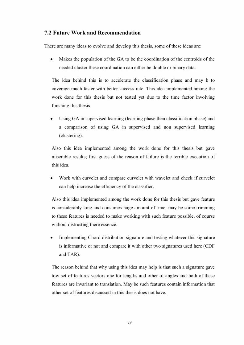
79

7.2 Future Work and Recommendation

There are many ideas to evolve and develop this thesis, some of these ideas are:

Makes the population of the GA to be the coordination of the centroids of the

needed cluster these coordination can either be double or binary data:

The idea behind this is to accelerate the classification phase and may b to

coverage much faster with better success rate. This idea implemented among the

work done for this thesis but not tested yet due to the time factor involving

finishing this thesis.

Using GA in supervised learning (learning phase then classification phase) and

a comparison of using GA in supervised and non supervised learning

(clustering).

Also this idea implemented among the work done for this thesis but gave

miserable results; first guess of the reason of failure is the terrible execution of

this idea.

Work with curvelet and compare curvelet with wavelet and check if curvelet

can help increase the efficiency of the classifier.

Also this idea implemented among the work done for this thesis but gave feature

is considerably long and consumes huge amount of time, may be some trimming

to these features is needed to make working with such feature possible, of course

without distrusting there essence.

Implementing Chord distribution signature and testing whatever this signature

is informative or not and compare it with other two signatures used here (CDF

and TAR).

The reason behind that why using this idea may help is that such a signature gave

tow set of features vectors one for lengths and other of angles and both of these

features are invariant to translation. May be such features contain information that

other set of features discussed in this thesis does not have.

80

Applying tree classification; since separating normal than abnormal has very

high success rate, clustering the abnormal cases to three categories directly.

Highest success rate obtained in this thesis came from classifying the cells into

just two categories (normal and abnormal) may be after this classification,

classifying abnormal cell into specific abnormal morphological gave better

result.

Besides the classifying normal, abnormal (sickle cell, burr cell and Teardrop)

increase the number of abnormal morphological in hand to includes other

shapes.

The four categories/ classes mentioned and targeted in this thesis is just the

start, blood morphological abnormalities shapes has no limit. May be working

with third dimension help in identifying some abnormalities where the cells

for example have spherical shapes which cannot be detected easily in two

dimension images. Finding ways to capture 3-dimention images under the

poor equipments found in here is discovery by itself.

81

Appendix

82

Appendix A. Classification of RBC Morphologic Abnormalities

The following table [52] gives details of the connection between the red blood cells

abnormality shapes and the diseases that related to it.

Table A.1 Classification of RBC Morphologic Abnormalities

RBC Abnormality Description of Cells Associated Conditions

Normal erythrocytes

("Discocytes,"

"normocytes")

Round to slightly ovoid

biconcave disks,

approximately 7 m in

diameter. Less hemoglobin in

center of cell (zone of

pallor). Regular in size and

shape.

Normal individuals.

Acanthocyte

("Spur cells")

Spheroid RBCs with few

large spiny projections. 5-10

spicules, irregular spacing

and thickness (must be

differentiated from

echinocytes).

Abetalipoproteinemia, postsplenectomy,

alcoholic cirrhosis and hemolytic anemia,

microangiopathic hemolytic anemia,

autoimmune hemolytic anemia,

sideroblastic anemia, thalassemia, severe

burns, renal disease, pyruvate kinase

deficiency, McLeod phenotype, infantile

pyknocytosis, post-splenectomy.

Autoagglutination Irregular RBC

agglutination/clumping

resembling Chinese letters.

Anti-RBC antibody, paraprotein. Cold

agglutinin disease, autoimmune hemolytic

anemia, macroglobulinemia,

hypergammaglobinemia

Basophilic stippling Fine, medium, or coarse blue

granules uniformly

distributed throughout RBC.

Fine stippling -

polychromatophilia. Coarse

stippling - Impaired

erythropoiesis.

Heavy metal poisoning (e.g. lead and

arsenic), hemoglobinopathies,

thalassemias, sideroblastic anemias,

pyrimidine-5’-nucleotidase deficiency

Bite cells RBCs with peripheral single Oxidant stress. Normal individuals

83

("Degmacytes") or multiple arcuate defects.

Usually associated with

spherocytes and blister cells.

receiving large quantities of aromatic drugs

(or their metabolites) containing amino,

nitro, or hydroxy groups. Individuals with

red-cell enzymopathies involving the

pentose phosphate shunt (most notably

G6PD deficiency.

Blister cells RBCs with vacuoles or

markedly thin areas at

periphery of membrane.

Glucose-6-phosphate dehydrogenase (G-6-

PD) deficiency. Other oxidant stress.

Codocytes

("Target cells")

Thin, hyopochromatic cell.

Round area of central

pigmentation.

Splenectomy, thalassemia,

hemoglobinopathies (hemoglobin SS, SC,

CC, EE, AE, sickle cell-thalassemia), iron

deficiency anemia, liver disease,

postsplectomy, familial lecithin-cholesterol

acyltransferase (LCAT) deficiency.

Dacrocytes

("Tear drops")

Cell in shape of tear drop.

Usually accompanied by

microcytosis and

hypochromia

Myelophthisic anemia (particularly

myelofibrosis with myeloid metaplasia),

magaloblastic anemia, b-thalassemia,

anemia of renal failure, tuberculosis, Heinz

body disease, hemolytic anemias,

hypersplenism.

Drepanocytes

("Sickle cells")

Irregular, curved cells with

pointed ends

Hb S hemoglobinopathies (sickle cell

anemia, hemoglobin SC disease,

hemoglobin S-beta-thalassemia,

hemoglobin SD disease, hemoglobin

Memphis/S disease), other

hemoglobinopathies (especially Hb I, Hb

CHarlem, HbCCapetown).

Echinocytes

("Sea urchin cells,

crenated cells, burr

cells")

RBC with many tiny spicules

(10-30) evenly distributed

over cell

Post-splenectomy, uremia, hepatitis of the

newborn, malabsorption states, after

administration of heparin, pyruvate kinase

deficiency, phosphoglycerare kinase

deficiency, uremia, HUsS.

84

Elliptocytes RBCs with elliptical or oval

shape

Hereditary elliptocytosis, thalassemia,

sickle cell trait, Hb C trait, cirrhosis,

decreased erythrocyte glutathione, glucose-

6-phosphate deficiency, iron deficiency

anemia, megaloblastic anemia,

myelophthisic anemia, hereditary

hemorrhagic telangiectasia, mechanical

trauma.

Howell-Jolly bodies Small (1 mm), round, dense,

basophilic bodies in RBCs.

Splenectomized patients, megaloblastic

anema, severe hemolytic processes,

hyposplenism, myelophthistic anemia.

Hyperchromia Increased RBC hemoglobin

concentration (MCHC > 36

g/dL). Usually associated

with spherocytosis

Hereditary spherocytosis, immune

hemolytic anemias.

Hypochromia Decreased RBC amount

(MCH) and concentration

(MCHC). Expanded central

zone of pallor

Iron deficiency, other hypochromic

anemias.

Keratocytes

("Horn cells")

Helmet forms Mechanical damage to red blood cells from

fibrin deposits (DIC, microangiopathic

hemolytic anemia, thrombotic

thrombocytopenic purpura), prosthetic

heart valves, severe valvular stenosis,

malignant hypertension, or march

hemoglobinuria, normal newborns,

bleeding peptic ulcer, aplastic anemia,

pyruvate kinase deficiency, vasculitis,

glomerulonephritis, renal graft rejection,

severe burns, iron deficiency, thalassemias,

myelofibrosis with myeloid metaplasia,

hypersplenism

85

Macrocyte

"Thin" macrocyte

Large RBCs (> 8.5 mm,

MCV > 95 fL). Normal

MCH

Increased diameter, normal

MCV. Usually hypochromic

Accelerated erythrocytosis. Macrocytic

anemia (B12 or folate deficiency)(oval

macrocytes)

Liver disease, postsplenectomy

Microcyte Small RBCs (< 7.0 mm, < 80

fL). Normal or decreased Hb

Iron deficiency, thalassemias, anemia of

chronic disease, lead poisoning,

sideroblastic anemia

Nucleated red blood

cells ("NRBCs")

Immature RBCs, basophilic

nucleus.

Acute bleeding, severe hemolysis,

myelofibrosis, leukemia, myelophthisis,

asplenia.

Poikilocytosis Variation in RBC shape. Many disorders.

Polychromasia

("Polychromatophilia")

Blue-gray coloration of

RBCS. Due to mixture of

RNA and hemoglobin.

Increased - Increased erythropoietic

activity. Decreased - Hypoproliferative

states.

Rouleaux Linear arrangement of

RBCs,"coinstack." Increased

fibrinogen, globulins, or

paraproteins (compare with

autoagglutination, above).

Acute and chronic inflammatory disorders,

Waldenstroms macroglobulinemia,

multiple myeloma.

Schistocytes

("Fragmented cells")

Fragmented RBCs (compare

with keratocytes, above)

Mechanical damage to red blood cells from

fibrin deposits (DIC, microangiopathic

hemolytic anemia, thrombotic

thrombocytopenic purpura), prosthetic

heart valves, severe valvular stenosis,

malignant hypertension, or march

hemoglobinuria, normal newborns,

bleeding peptic ulcer, aplastic anemia,

pyruvate kinase deficiency, vasculitis,

glomerulonephritis, renal graft rejection,

severe burns, iron deficiency, thalassemias,

myelofibrosis with myeloid metaplasia,

86

hypersplenism

Spherocytes RBCs with spheroidal shape.

Usually dense, small (< 6.5

mm) RBCS with normal or

decreased MCV, and absent

central pallor

Hereditary spherocytosis and hemolytic

anemias (isoimmune or autoimmune),

microangiopathic hemolytic anemia,

hypersplenism and post-splenectomy,

myelofibrosis with myeloid metaplasia,

hemoglobinopathies, malaria, liver disease,

older population of transfused cells,

artifact. Microspherocytes in severe burns

and hereditary pyropoikilocytosis.

Stomatocyte

(Fish mouth cell")

Uniconcave RBC, slitlike

area of central pallor

Hereditary or acquired hemolysis.

Hereditary stomatocytosis, alcoholic

cirrhosis, acute alcoholism, obstructive

liver disease, malignancy, severe infection,

treated acute leukemia, artifact.

87

Appendix B. Blood Films Preparation

Blood films are made by placing a drop of blood on one end of a slide, and using a

spreader slide to disperse the blood over the slide's length [52]. The aim is to get a

region where the cells are spaced far enough apart to be counted and differentiated.

The slide is left to air dry, after which the blood is fixed to the slide by immersing it

briefly in methanol. The fixative is essential for good staining and presentation of

cellular detail. After fixation, the slide is stained to distinguish the cells from each

other.

MATERIALS

- Sterilized lancets or needles

- 20 clean microscope slides and coverslips

- Canada balsam or other medium for permanent preparations

- 95% ethyl or methyl alcohol

- Distilled water

- Giemsa stain or other.

- Low containers or Petri dishes.

- Microscope which magnifies 200 times at least

Taking the Blood

Cleanse a finger. With a sterile lancet, make a puncture on a fingertip. keep all

the materials needed ready and protected from dust, particularly the clean microscope

slides.

Making the Smear

Place a small drop of blood near an end of a slide. According to figure 7, bring

the edge of another slide in contact with the drop and allow the drop to bank evenly

behind the spreader. The angle between the two slides has to be 30-40 degrees. Now,

push to the left in a smooth, quick motion. The smear should cover about half the

slide. It is important that the quantity of blood is not excessive; otherwise the red cells

could hide the leukocytes. So, if you succeed in making a gradual transition from

thick to thin in your smear, you should get a zone with a satisfactory distribution of

cells. With a single drop of blood, you can make several smears.

88

In fact, to make a smear, it is enough to leave a spot of blood of 3 mm about in

diameter on the slide. It is useful to perform many smears. In fact, not always they are

successful, and with some attempts, it is easier to get one well prepared. To avoid

producing clots, you must make each smear with fresh blood and straight after having

deposited it. To this purpose, it is useful to be helped by another person where one

deposits the blood, and the other makes the smears. With the microscope, you should

observe the smears to check that some of them are properly made. The red cells must

not overlap each other, nor be so scarce as to be too spread out.

Fixing

If you apply the stain to a smear without having fixed it beforehand, the cells will

explode because of the so-called osmotic or hypotonic shock. This happens because

the saline concentration inside the cells is much higher than that of staining fluid

which is diluted in distilled water. In the attempt to equal the internal saline

concentration to the values of the external one, the cells undergo swelling by osmosis.

To attain the same saline concentration of the external liquid, the cells should swell

more than their membrane allows, in fact they explode. The cell contents are released,

and the preparation becomes unusable. To avoid this, before staining, you have to fix

the smear. This operation hinders the inflation of the cells which keep sound when

they are stained. A simple and effective fixing technique consists of dipping the smear

Figure B.1. Prepare blood smear

89

in a vessel containing 95% ethyl or methyl alcohol for 3-5 minutes. In order to put

alcohol on the smear, you can also use a dropper or a bottle dispenser.

Staining

If you observe the smear as it is after fixing, you will see very little because all cells

are very transparent. The erythrocytes are slightly visible, but the leukocytes are too

pale, almost invisible and you will not see anything inside them. To be able to observe

and recognize the different kinds of leukocyte, you must stain them. For this purpose,

normally Giemsa stain is used. It is a mixture of stains, based on methylene blue and

eosin. It is cheaply available commercially in volumes of 100 cc. It consists of a

concentrated solution which you have to dilute in the proportion1/10, that is one part

of Giemsa in nine of distilled water, or buffer solution (pH = 6,8-7,2). You can buy

the stain in a store of chemicals and laboratory equipment.

To stain a smear, take a slide with a fixed and dry smear. Put on the slide a drop of

stain until it is fully covered. Stain for about 16 minutes, renewing the stain about four

times. Then rinse the slide with distilled water at room temperature. Drain off the

water and leave the slide to dry.

Checking

With the microscope, verify that the cells are well stained. If necessary, apply the

stain for a few more minutes. If you were planning to mount the slide with Canada

balsam, the staining has to be stronger.

Cover-Slipping

At this point, your smear is ready to be observed, but if you want to keep it for a long

time, you should make the preparation permanent. To this purpose, after drying the

slide, place a drop of Canada balsam or another medium mountant on the smear,

then mount the coverslip. If the balsam is too viscous, you may heat a few of the

slides (but not over 40 degrees C) to help the balsam flow between the slide and

coverslip.

90

Observation

A magnification of 200 times is enough to allow you to observe and identify the

different types of cells. If you use a higher power, you can also see the cells details

better. You can examine either with dry objectives or with the oil immersion

technique. In this last case, if you have put on a coverslip, you must wait a day to

allow the balsam to set, otherwise, when you move the slide, oil will displace the

coverslip.

91

Biography [1] J. H. Carr, Bernadette F. Rodak, Clinical hematology Atlas, Saunders Elsevier, 3rd Ed, 2009, pp.222-230.

[2] N. C.Jain, Essentials of Veterinary Hematology, Lea & Febiger.Philadelphia, 1st Ed, 1993, pp.312-32.,

[3] L. Williams and Wilkins, Blueprints Hematology and Oncology, Blackwell.Massachusetts, 1st Ed, 2005, pp. 220-231.

[4] E. c. Besa, P. M. Catalano and J. A. Kant, The National Medical Series of Independent Study Hematology, 1992, Lippincott Williams & Wilkins, pp.222-223.

[5] N. Beck, “Diagnostic Hematology,” Springer.Londom, 1st Ed, 2009, pp. 520-536.

[6] G. Karkavitsas and M. Rangoussi, "Object Localization in medical images using genetic algorithm, " World academy of Science, Engineering and Technology, vol. 2, pp. 6-9, Feb. 2005.

[7] P.J.H. Bronkorsta a, M.J.T. Reinders b, E.A. Hendriks b, J. Grimbergen a, R.M. Heethaar c, G.J. Brakenho, "On-line detection of red blood cell shape using deformable Templates, " Elsevier Science, vol. 3, pp. 413-424, Jan. 2000.

[8] E. Ozcan and C. K. Mohan, " Partial shape matching using genetic algorithms, " Elsevier Science, vol.18, Oct. 1997.

[9] N. Guil, J. M. Gonzalez-Linares and E. L. Zapata, " Bidimensional shape detection using an invariant approach ", Elsevier Science B.V, vol.32, issue 6, pp.1025-1038, June.1999.

[10N. Guil and E.L. Zapata , "Lower Order Circle and Ellipse Hough Transform", Pattern Recognition, vol. 30, no. 10, pp.1729-1744, October.1997.

[11] N. Guil, J. Villalba and E.L. Zapata, "A Fast Hough Transform for Segment Detection", IEEE Transaction on Image Processing, vol. 4, no.11, pp.1541-1548, November.1995.

[12] P. Ghosh and M. Mitchell, " Segmentation of Medical Images Using a Genetic Algorithm," on the 8th annual conference on Genetic and evolutionary computation, pp.1171 -1178, 2006.

[13] K. Muthukannan, " Color image segmentation using k-means clustering and Optimal Fuzzy C-Means clustering ," Communication and Computational Intelligence International Conference, Erode, 2010, pp.229-234.

[14] R. Kalam, " Enhancing K-Means Algorithm for Image Segmentation," in Process Automation, Control and Computing International Conference, Coimbatore, India, 2011, pp.1-4.

[15] M. Rizon, H.Yazid, P. Saad, A. Yeon Md Shakaff, A. Saad , M. Sugisaka, S. Yaacob, M.Rozailan Mamat and M. Karthigayan. " Object Detection using Circular Hough Transform," American Journal of Applied Sciences, vol.12, pp 1606-1609, Jan. 2005.

[16] K. Fukui and O. Yamaguchi, "Facial feature points extraction method based on combination of shape extraction and pattern matching," Trans. IEICE, Vol.8, pp.2170-2177, 1997.

92

[17] D. L. Pham, C. Xu, J. L, Prince, “Survey of current methods in medical image segmentation,” Annual Review of Biomedical Engineering, Vol. 2, pp. 315-337, 2000.

[18] T. M. Mitchell, "Machine Learning," in Machine learning, McGraw Hill, 1997.

[19] J. Holland, " Adaptation in natural and artificial systems," University of Michigan Press, Ann Arbor, pp.15-15, August.1975.

[20] M. Mitchell, "An introduction to genetic algorithms," Artificial Intelligence. Cambridge, MA:MIT Press, 1996. [15] D. E. Goldberg, "Genetic algorithms in search," optimization and machine learning, 1st Ed. , Addison-Wesley Longman, 1989.

[21] C. Harris and B. Buxton, "Evolving edge detectors," Research not, RN/96/3, University College London, Dept. of Computer Science, London, 1996

[22] N. Harvey, J. Theiler, S. P. Brumby, S. Perkins, J. J. Szymanski, J. J. Bloch, R. B. Porter, M. Galassi and A. C. Young, "Comparison of GENIE and conventional supervised classifiers for multi-spectral image feature extraction, " IEEE Trans. Geosci. Remote Sens, vol. 40, no. 2, pp. 393 – 404, Feb. 2002.

[23] P. Nordin and W. Banzhaf, "Programmi0ng compression of Images and sound," in genetic programming, In: Koza JR et al (eds) , Proceedings of the 1st annual conference, Morgan Kaufmann, San Francisco,1996, pp. 345-350.

[24] D. E. Goldberg, "Genetic algorithms in search," optimization and machine learning, 1st Ed. , Addison-Wesley Longman, 1989.

[25] L. Ballerini, "Genetic snakes for medical images segmentation," In: Poli R et al. (eds) Proceedings of the first European workshops on evolutionary image analysis, signal processing and telecommunications, Lecture notes in computer science, 1596. Springer-Verlag, London, 26–27, may, 1999, pp. 59-73.

[26] A. Hill, C. Taylor, "Model-based image interpretation using genetic algorithms". Image Vis Comput., Vol.10, pp.295–300, 1992.

[27] Hindawi, L. MacEachern, T. Manku, "Genetic algorithms for active contour optimization". IEEE Proc Intl Symp Circuits Sys, Vol.4, pp.229– 232, 1998.

[28] R. Poli and S. Cagoni, "Genetic programming with user-driven selection: experiments on the evolution of algorithms for image enhancement," in the 2nd Annual conference on Genetic programming, pp.269-277, 1997.

[29] N. Harvey, RM. Levenson, DL. Rimm, "Investigation of automated feature extraction techniques for applications in cancer detection from multi-spectral histopathology images". Proc SPIE, Vol.5032, pp.557–566, 2003.

[30] S. Perkins, J. Theiler, SP Brumby, N. R Harvey, RB Porter, JJ Szymanski, JJ Bloch, "GENIE: a hybrid genetic algorithm for feature classification in multi-spectral images," Proc. SPIE 4120, pp. 52- 62, 2000.

[31] C. Lin and J. Wu, "Automatic Facial Feature Extraction by Genetic Algorithms," IEEE Trans. Imag. vol.8. no 6. pp. 834-888, Jun. 1999.

[32] Y. Fan, T. Jiang and D. J. Evans, "Volumetric Segmentation of Brain Images Using Parallel Genetic Algorithms," IEEE Trans. Med. Imag, vol. 21, no. 8, pp. 905-910, Aug. 2002.

93

[33] S. Cagnoni, A. B. Dobrzeniecki, R. poli and J. C.Yanch, "Genetic algorithm-based interactive segmentation of 3D medical images," Elsevier B.V. Image Vis Comput, vol. 17, no. 12, pp. 881–895, Sep. 1999.

[34] J. Goldberger, H. Greenspan, "Context-based segmentation of image sequences,". IEEE Trans Patt Ana Mach Intell, vol. 28, no. 3, pp. 463– 468, Jan. 2006.

[35] C. Harris and B. Buxton, "Evolving edge detectors. Research note RN/96/3," University College London, Dept. of Computer Science, London, 1996.

[36] K. I. Laws, "Texture image segmentation". PhD. dissertation, University of Southern California, 1980.

[37] A. Termeau and N. Borel, " A region growing and merging algorithm to color segmentation," Pattern Recogn., vol. 30, no. 7, pp. 1191- 1203, July, 1997.

[38] B. Bhanu, S. Lee and J. Ming, "Adaptive Image Segmentations Using Genetic algorithm, " IEEE Trans. Man. Cybernetics, vol. 25, no. 12. pp.543- 1555, Dec. 1995.

[39] S. Bandyopadhyay, C. A. Murthy, and S. K. Pal, “Pattern classification with genetic algorithms,” Pattern Recogni. Lett., vol. 16, 1995, pp. 801–808.

[40] C. A. Murthy and N. Chowdhury, “In search of optimal clusters using genetic algorithm,” Pattern Recognit. Lett., vol. 17, 1996, pp. 825–832.

[41] S. K. Pal and P. P. Wang, "Genetic Algorithms for Pattern Recognition," in Pattern Recognit. lett, Boca Raton, FL: CRC Press, 1996.

[42] H. J. Lin, F. W. Yang and Y. T. Kao, "An Efficient GA-based Clustering Technique," Tamkang Journal of Science and Engineering, vol.8, Jan. 2005, pp.113-122.

[43] A. Kamble, "Incremental Clustering in Data Mining using Genetic Algorithm," International Journal of Computer Theory and Engineering, vol.2, Jun. 2010, pp.1793-8201.

[44] K. Krishna and M. N. Murty, " Genetic K-Means Algorithm," IEEE TRANS.MAN. SYS, vol.29, Jun.1999, pp.433-439.

[45] D. K. Roy and L. K. Sharma, "Genetic K-Means Clustering Algorithm for Mixed Numeric and Categorical Data Sets," International Journal of Artifical Intelligence and Applications (IJAI), vol.1, April. 2010, pp.23-28.

[46] Peng-Yeng Yin, Pattern Recognition Techniques, Technology and Application, Veinna, Austria, Nov. 2008, pp.626.

[47] J. M. Black, J. H. Hawks, Medical-Surgical Nursing, Saunders, 1st Ed, Vol.1, 2009.

[48] K. D. McClatchey, Clinical laboratory medicine, Lippincott Williams & Wilkins , 2nd Ed, 2002.

[49] P.R. Wheater, H.G. Burkitt and V.G. Daniels, Functional Histology, Longman Group.UK, 2nd Ed, 1987

[50] J. M. Black, J. H. Hawks. Medical-Surgical Nursing, Saunders, 1st Ed, Vol.1, 2009.

[51] M. E. Feder, Environmental Physiology of the Amphibians, Uiv.Chicago Press, 1st Ed, 1992.

[52] J. P. Greer and M. M. Wintrobe, Wintrobe's Clincal Hematology, Lppincott Williams and Wilkins, Vol. 1, 2008.

94

[53] S. Theodoridis and K. Koutroumbs, " Pattern Recognition," Elsevier Inc.Academic Press, 4th Ed, 2009.

[54] R. Gonzalez and R. Woods Digital Image Processing, Addison-Wesley Publishing Company, 1992, pp 518 – 548.

[55] R. Haralick and L. Shapiro Computer and Robot Vision, Vol. 1, Addison-Wesley Publishing Company, 1992, ch. 5, pp 168 – 173.

[56] A. Jain, Fundamentals of Digital Image Processing, Prentice-Hall, 1989, ch. 9.

[57] S. Han and S. Yang, “An invariant feature representation for shape retrieval,” in Proc. Sixth International Conference on Parallel and Distributed Computing, Applications and Technologies, 2005.

[58] L. J. Latecki and R. Lakamper, “Convexity rule for shape decomposition based on discrete contour evolution,” Computer Vision and Image Understanding, vol. 3, issue.3 pp. 441- 454, 1999.

[59] T. Sebastian, P. Klein, and B. Kimia, “Recognition of shapes by editing their shock graphs,”IEEE Trans. Pattern Analysis and Machine Intelligence, vol. 26, pp. 550-571, 2004.

[60] W. Klimesch, "EEG alpha and theta oscilliations reflect cognitive and memory performance: a review and analysis," 1st ed. Barin Res. 1999, pp.169-195.

[61] L. Berger, J.C. Morris, Diagnosis in Alzheimer Disease, 1st ed. New York, Reaven Press, 1994, pp. 9-25.

[62] A. Gorea, "Representations of Vision," Cambridge University Press, Apr.1991.

[63] E. Maeland, “On the comparison of interpolation methods,” IEEE Trans. Med. Imag., vol. 7, no. 3, pp. 213–217, Sept.1988.

[64] J. L. Ostuni, A. K. S. Santha, V. S. Mattay, D. R. Weinberger, R. L. Levin, and J. A. Frank, “Analysis of interpolation effects in the reslicing of functional MR images,” J. Comput. Assist. Tomogr., vol. 21, no. 5, pp. 803–810, 1997.

[65] R.W. Parrot, M. R. Stytz, P. Amburn, and D. Robinson, “Toward statistically optimal interpolation for 3-D medical imaging,” IEEE Eng. Med. Biol., vol. 12, no. 5, pp. 49–59, Sept.–Oct. 1993.

[66] M. Haddad and G. Porenta, “Impact of reorientation algorithms on quantitative myocardial SPECT perfusion imaging,” J. Nucl. Med., vol. 39, no. 11, pp. 1864–1869, Nov. 1998.

[67] B. Migeon and P. Marche, “In vitro 3D reconstruction of long bones using B-scan image processing,” Med. Biol. Eng. Comput., vol. 35, no. 4, pp. 369–372, July 1997.

[68] M. R. Smith and S. T. Nichols, “Efficient algorithms for generating interpolated (zoomed) MR images,” Magn. Reson. Med., vol. 7, no. 2, pp. 156–171, June.1988.

[69] S. D. Fuller, S. J. Butcher, R. H. Cheng, and T. S. Baker, “Three-dimensional reconstruction of icosahedral particles - The uncommon line,” J. Struct. Biol., vol. 116, no. 1, pp. 48–55, Jan.–Feb. 1996.

[70] F. M.Weinhaus and V. Devarajan, “Texture mapping 3D models of real world scenes,” ACM Comput. Surv., vol. 29, no. 4, pp. 325–365, Dec. 1997.

95

[71] T. Möller, R. Machiraju, K. Mueller, and R. Yagel, “Evaluation and design of filters using a Taylor series expansion,” IEEE Trans. Visual. Comput. Graph., vol. 3, no. 2, pp. 184–199, Apr–June.1997

[72] C. R. Appledorn, “A newapproach to the interpolation of sampled data,” IEEE Trans. Med. Imag., vol. 15, no. 3, pp. 369–376, June.1996.

[73] N. A. Dodgson, “Quadratic interpolation for image resampling,” IEEE Trans. Image Processing, vol. 6, no. 9, pp. 1322–1326, Sept. 1997.

[74] I. German, “Short kernel fifth-order interpolation,” IEEE Trans. Signal Processing, vol. 45, no. 5, pp. 1355–1359, May 1997.

[75] F. J. Harris, “On the use of windows for harmonic analysis with the discrete Fourier transform,” Proc. IEEE, vol. 66, no. 1, pp. 51–83, Jan. 1978.

[76] R. G. Keys, “Cubic convolution interpolation for digital image processing,” IEEE Trans. Acoust., Speech, Signal Processing, vol. ASSP-29, no. 6, pp. 1153–1160, Dec. 1981.

[77] E. H.W. Meijering, K. J. Zuidervel, and M. A. Viergever, “Image reconstruction with symmetrical piecewise nth-order polynomial kernels,” IEEE Trans. Image Processing, vol. 8, no. 2, pp. 192–201, Feb. 1999.

[78] G. Wolberg, "Digital Image Warping," IEEE Computer Society Press, Los Alamitos, California, 1990.

[79] M. Unser, "Splines – A Perfect Fit for Signal and Image Processing," IEEE Signal Processing Magazine, pp. 22-38, 1999.

[80] R. G. Keys, "Cubic Convolution Interpolation for Digital Image Processing," IEEE Transactions on Acoustics, Speech, and Signal Processing, Vol. 29, pp.1153-1160, 1981.

[81] A. K. Maini and V. Agrawal, "satellite Technology, " John Wiley and Sons, Jan.2007,pp.365.

[82] G. Gan, C. Ma, J. Wu, "Data ClusteringTheory, Algorithms,and Applications," SIAM(Society for Industrial and Applied Mathematics), 2007.

[83] J. MacQueen. "Some methods for classification and analysis of multivariate observations," on the 5th Berkeley symposium on mathematical statistics and probability, 1967, pp. 281-297.

[84] W. Barbakh, Y. Wu, and C. Fyfe, Non-standard parameter adaptation for exploratory data analysis, Springer, 2009

[85] M. A. Abed, A. N. Ismail and Z. M. Hazi , "Pattern Recognition Using Genetic Algorithm," International Journal of Compute and Electrical Engineer, Vol. 3, No.3, 2010, pp 1793-8163.

[86] V. V. Raghavan and K. Birchand, “A Clustering Strat Strategy Based on a Formalism of the Reproductive Process in a Natural System,” in the 2nd International Conference on Information Storage and Retrieval, pp. 10-22, 1979.

[87] D. Jones and M. A. Beltramo, “Solving Partitioning Problems with Genetic Algorithms,” in Proceedings of the 4th International Conference on Genetic Algorithms, pp. 442-449 , 1991

96

[88] G. P. Babu and M. N. Murty, “Clustering with Evolution Strategies,” Pattern Recognition, Vol. 27, pp. 321- 329, 1994.

[89] U. Maulik and S. Bandyopadhyay, “Genetic Algorithm- Based Clustering Technique,” Pattern Recognition, Vol. 33, pp. 1455, 2000.

[90] S. Bandyopadhyay and U. Maulik, “Genetic Clustering for Automatic Evolution of Clusters and Application to Image Classification,” Pattern Recognition, Vol. 35, pp. 1197-1208, 2002.

[91] JH. Holland, " Adaptation in natural and artificial systems," University of Michigan Press, Ann Arbor, pp.15-15, August.1975

[92] P. Kohn, "Combing Genetic Algorithm and Neural Networks" M.Sc. thesis, Tennessee Unive,1994

[93] P. Kohn, "Combing Genetic Algorithm and Neural Networks" M.Sc. thesis, Tennessee Unive,1994

[94] Sh. A. Rasheed, "Genetic Algorithms Application in Pattern Recognition," M.Sc. thesis, National Computer Center Higher Education Institute, 2000.

[95] R. L. Wainwright, "Introduction to Genetic Algorithms Theory and Applications",Addison-Wesley, 1993.

[96] M. Schamidt and T. Stidsen, "Hybrid Systems: Genetic Algorithms, Neural Network and Fuzzy logic ," Univ. Aarhus .Denmark, 1997.

[97] P. Franti, J. Kivjarvi, T. Kaukoranta and O. Nevalainen. "Genetic Algorithm for Large- Scale Clustering Problems," The Computer Journal, Vol.40, no.9, 1997.

[98] M. L. Mauldin, "Maintaining Diversity in Genetic Search," The National Conference on Artificial Intelligence (AAAI- 84), August.1984.

97

حتديد أشكال خاليا الدم احلمراء املريضة باستخدام اجلينات اخلوارزمية والكي مينز

ات العليا ـــتري يف كلية الدراســـات نيل درجة املاجســزء من متطلبـــــــرسالة مقدمة كجوبـــــة احلاســــة ختصص هندســــم اهلندســـقس

:اعداد

فاتن فرج ابومشالة/ ةــاملهندس

:رافــــــــاش

د امحد احلنجوريـــحمم/ املهندس .الدكتور

غزة، فلسطین

(1433ھـ ,2012)

وبـــــــالحاس ةــــــــــھندس قسم ةـــــــــــــــــالھندس كلیة

العلیا اتـــــــــــــــالدراس عمادة غزة – المیةاإلس الجامعة

طینـــــــــــــــــــــفلس

98

إهداء

99