Detecting Mean Reverted Patterns in Statistical Arbitrage

Kostas TriantafyllopoulosUniversity of Sheffield

OutlineI Motivation / algorithmic pairs trading

I Model set-upI Detection of local mean-reversion

I Adaptive estimationI 1. RLS with gradient variable forgetting factorI 2. RLS with Gauss-Newton variable forgetting factorI 3. RLS with beta-Bernoulli forgetting factor

I Trading strategy

I Pepsi and Coca Cola example

Introduction

I Statistical arbitrage.

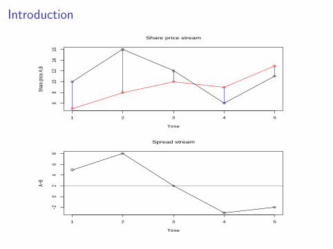
I Algorithmic pairs trading market neutral trading.Buy low, sell high.

I Two assets with prices pAt and pBtI At t: if pAt < pBt , buy low (A) and sell high (B).I At t + 1: if pAt > pBt , buy low (B) and sell high (A)...

I In the long run, mean reversion of spread yt = pAt − pBt .If yt goes up, yt will go down at t + 1.Take advantage of relative mispricings of A and B.

Introduction

Share price stream

Time

Shar

e pric

e A,B

1 2 3 4 5

68

1012

1416

Spread stream

Time

A−B

1 2 3 4 5

−20

24

68

Pepsi - Coca Cola date stream

Trading day

Shar

e Pric

es (in

USD

)

2002 2004 2006 2008 2010 2012

4050

6070

80 Pepsi

Coca−Cola

2004 2006 2008 2010

−10

05

1020

−−−− Mean of Spread =7.365

Model set-up

(Elliott et al, 2005). yt is a noisy version of a mean-revertedprocess.

yt = xt + εt

xt = α+ βxt−1 + ζt

(Triantafyllopoulos and Montana, 2011).

yt = αt + βtyt−1 + ϵt = FTt θt + ϵt ,

θt = Φθt−1 + ωt ,

Ft =

[1

yt−1

]and θt =

[αt

βt

]

Detecting mean reversion

Define Dt = (y1, . . . , yt) a data stream sample.

I (Elliott et al, 2005).If |β| < 1, then yt is mean-reverted.With Dt , get online estimates α and β. If |β| < 1, thenmean-reversion.

I (Triantafyllopoulos and Montana, 2011).Under some assumptions yt is mean-reverted if |βt | < 1, forall t. We consider mean-reversion in segments or locally.Test again |βt | < 1.

So we need online estimates βt .

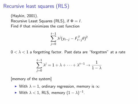
Recursive least squares (RLS)

(Haykin, 2001).Recursive Least Squares (RLS), if Φ = I .Find θ that minimizes the cost function

t−1∑j=0

λj(yt−j − FTt−jθ)

2

0 < λ < 1 a forgetting factor. Past data are “forgotten” at a rate

t−1∑j=0

λj = 1 + λ+ · · ·+ λt−1 → 1

1− λ

[memory of the system]

I With λ = 1, ordinary regression, memory is ∞I With λ < 1, RLS, memory (1− λ)−1.

SS-RLS (state-space RLS)

Variable forgetting factor (Haykin, 2001, Malik, 2006).

λt − λt−1 = c(t)

Steepest descent:

λt = [λt−1 + a∇λ(t)]λ+

λ−,

1. ∇λ(t) ≈ −etFTt Φψt−1

2. ψt = ∂mt/∂λ = (I − KtFTt )Φψt−1 + StFtet

3.

St = ∂Pt/∂λ = −λ−1t Pt + λ−1

t KtKTt

+λ−1t (I − KtF

Tt )ΦSt−1Φ

T (I − FtKTt ).

Need starting values m1,P1, ψ1,S1, λ1.

GN-RLS (Gauss-Newton RLS)Song et al (2000) gave an approximate GN algorithm.

λt =

[λt−1 + a

∇λ(t)

∇2λ(t)

]λ+

λ−

,

Here ∇2λ(t) ≈ (FT

t Φψt−1)2 − etF

Tt Φηt

ηt = ∂ψt−1/∂λ = (I − KtFTt )Φηt−1 + LtFtet − 2StFtF

Tt Φψt−1

where

Lt = λ−1t (I − KtF

Tt )ΦLt−1Φ

T (I − FtKTt )

+λ−2t Pt(I − FtK

Tt )− λ−1

t St +Mt +MTt

−λ−2t (I − KtF

Tt )ΦSt−1Φ

T (I − FtKTt )

and

Mt = λ−1t StFtF

Tt {Pt − ΦSt−1Φ

T (I − FtKTt )}.

GN-RLS cont.

I GN-RLS creates too abrupt jumps in λt / too sensitive tochanges.

I When smooth signal, we want SS-RLS and when noisy wewant GN-RLS.

I We use

λt =

[λt−1 + a∇λ(t)]λ+λ− , if e2t ≤ k[

λt−1 + a∇λ(t)∇2

λ(t)

]λ+λ−, if e2t > k

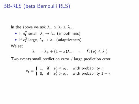
BB-RLS (beta Bernoulli RLS)

In the above we ask λ− ≤ λt ≤ λ+.

I If e2t small, λt → λ+ (smoothness)

I If e2t large, λt → λ− (adaptiveness)

We setλt = πλ+ + (1− π)λ−, π = Pr(e2t ≤ kt)

Two events small prediction error / large prediction error

xt =

{1, if e2t ≤ kt , with probability π0, if e2t > kt , with probability 1− π

Observation model xt ∼ Bernoulli(π).Prior for π is beta, π ∼ B(c1, c2)

p(xt | π) = πxt (1− xt)1−xt (bernoulli model)

p(π) ∝ πc1−1(1− π)c2−1 (prior beta model)

p(π | xt) ∝ p(xt | π)p(π) ∝ πc1+xt−1(1− π)c2+1−xt−1

So π|xt ∼ B(c1 + xt , c2 − xt + 1).Sequentially: π | x1, . . . , xt ≡ π | Dt−1 ∼ Be(c1t , c2t), wherec1t = c1,t−1 + xt and c2t = c2,t−1 − xt + 1.

πt = E (π | Dt−1) = c1t(c1t + c2t)−1

λt = E (λt |Dt−1) = πtλ+ + (1− πt)λ−

From Pr(e2t ≤ kt) = π, we have kt = qtF−1χ2 (π).

We use kt ≈ qtF−1χ2 (πt−1).

Key points of λt

I λt is stochastic.

I We can derive its distribution

p(λt |Dt−1) = c(λt − λ−)c1t−1(λ+ − λt)

c2t−1

I We can evaluate the mode and the variance of λt .

I We can showλt ≈ xλ+ + (1− x)λ−

I If for many points e2t < kt , followed by few large e2t > kt ,then locally λt does not work well.

Solution: intervention

Example.

1. Set λ− = 0.8, λ+ = 0.99

2. e2t ≤ kt (t = 1, . . . , 95)

3. e2t > kt (t = 96, 97, 98, 99, 100)

4. λt = 0.9805 (closer to λ+ = 0.99, than to λ− = 0.8).

If change in xt (from 0 to 1 or from 1 to 0), reset the priors c1,t−1

and c2,t−1 to the initial values (c1,1 = c2,1 = 0.5).

πt =c1t

c1t + c2t=

c1,1 + xtc1,1 + c2,1 + 1

=1 + 2xt

4

λt =

{0.75λ+ + 0.25λ−, if xt = 10.25λ+ + 0.75λ−, if xt = 0

In the example, λ96 = 0.25× 0.99 + 0.75× 0.8 = 0.847.

Simulated streams

Time

Simula

ted S

pread

300 320 340 360 380 400 420 440

05

10

Prediction of |Bt|

Trading day

300 320 340 360 380 400 420 440

0.20.4

0.60.8

1.0

SS−RLS

GN−RLS

BB−RLS

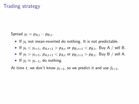
Trading strategy

Spread yt = pA,t − pB,t .

I If yt not mean-reverted do nothing. It is not predictable.

I If yt < yt+1, pA,t+1 > pA,t or pB,t+1 < pB,t . Buy A / sell B.

I If yt > yt+1, pA,t+1 < pA,t or pB,t+1 > pB,t . Buy B / sell A.

I If yt ≈ yt−1, do nothing.

At time t, we don’t know yt+1, so we predict it and use yt+1.

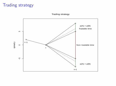
Trading strategy

−50

5

Trading strategysp

read

y

p(A) > p(B)

p(A) < p(B)

t−1

t

t+1

Tradable time

Non−tradable time

With observed spread yt at t:

I Close the position of t − 1 (if opened).

I If |βt+1| < 0.99, declare yt+1 as mean-reverted.

I If yt+1 − h > yt , buy A / short-sell B.

I If yt+1 + h < yt , buy B / short-sell A.

Example:

I At t: yt = 10 and we project yt+1 = 11.

I yt+1 can be 12 or 9 (rules change if we apply yt <> yt+1.

I yt+1 = 9 can give loss, if we adopt yt < yt+1 rule (10 < 11).

I Take h = 10% of yt+1 = 1.1, and yt+1 − h = 9.9 < 10 = yt ,we do not open a position buy A and short sell B.

I As yt+1 + h = 11.1 > 10 = yt , we do not open a positionshort sell A and buy B.

Pepsi - Coca Cola date stream

Trading day

Shar

e Pric

es (in

USD

)

2002 2004 2006 2008 2010 2012

4050

6070

80 Pepsi

Coca−Cola

2004 2006 2008 2010

−10

05

1020

−−−− Mean of Spread =7.365

Detection of mean reverted patterns

0.98

00.

990

1.00

01.

010

SS

−RLS

0.98

00.

990

1.00

01.

010

GN

−RLS

0.98

00.

990

1.00

01.

010

2002 2004 2006 2008 2010 2012

BB

−RLS

Trading day

Prediction of |Bt|

MSE over time

Mean square error of the three algorithms

Trading day

2002 2004 2006 2008 2010 2012

05

1015

2025

30

SS−RLS

GN−RLS

BB−RLS

Trading performance

h

Mean 1% 3% 5%

SS-RLS 35.758 30.860 30.655GN-RLS 101.885 92.819 80.091BB-RLS 119.935 97.140 64.146

STD 1% 3% 5%

SS-RLS 57.210 55.638 55.357GN-RLS 53.799 59.603 63.687BB-RLS 54.890 60.223 58.654

FB 1% 3% 5%

SS-RLS 131.85 129.29 127.85GN-RLS 155.19 159.44 172.29BB-RLS 185.28 178.58 155.00

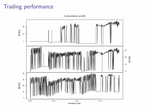
Trading performance

050

100

SS−R

LS

050

100

150

GN−R

LS

050

100

150

200

2008 2009 2010 2011

BB−R

LS

Trading day

Cumulative profit

Closing remarks

I Algorithmic pairs trading / statistical arbitrage require onlinemachine learning methods.

I Pattern recognition methods for mean reversion / segments ofstationarity.

I We develop variable forgetting factors for online learning.

I Other methods include sequential Monte Carlo.

I Need to take into account the shape of the distribution of thedata stream.

I Larger data streams / complex portfolios / many pairs toconsider simultaneously.

I Trading strategy can be improved.

References

I Elliott, R., Van Der Hoek, J., and Malcolm, W. (2005). Pairstrading. Quantitative Finance, 5:271-276.

I Haykin, S. (2001). Adaptive Filter Theory. Prentice Hall, 4thedition.

I Malik, M. B. (2006). State-space recursive least-squares withadaptive memory. Signal Processing, 86:1365-1374.

I Song, S., Lim, J.-S., Baek, S., and Sung, K.-M. (2000).Gauss-Newton variable forgetting factor recursive least squaresfor time varying parameter tracking. Electronics Letters,36:988-990.

I Triantafyllopoulos, K. and Montana, G. (2011). Dynamicmodeling of mean-reverting spreads for statistical arbitrage.Computational Management Science, 8:23-49.