Detecting Adversarial Samples from Artifacts

Reuben Feinman 1 Ryan R. Curtin 1 Saurabh Shintre 2 Andrew B. Gardner 1

AbstractDeep neural networks (DNNs) are powerful non-linear architectures that are known to be robustto random perturbations of the input. How-ever, these models are vulnerable to adversarialperturbations—small input changes crafted ex-plicitly to fool the model. In this paper, we askwhether a DNN can distinguish adversarial sam-ples from their normal and noisy counterparts.We investigate model confidence on adversarialsamples by looking at Bayesian uncertainty esti-mates, available in dropout neural networks, andby performing density estimation in the subspaceof deep features learned by the model. The resultis a method for implicit adversarial detection thatis oblivious to the attack algorithm. We evalu-ate this method on a variety of standard datasetsincluding MNIST and CIFAR-10 and show thatit generalizes well across different architecturesand attacks. Our findings report that 85-93%ROC-AUC can be achieved on a number of stan-dard classification tasks with a negative class thatconsists of both normal and noisy samples.

1. IntroductionDeep neural networks (DNNs) are machine learning tech-niques that impose a hierarchical architecture consisting ofmultiple layers of nonlinear processing units. In practice,DNNs achieve state-of-the-art performance for a variety ofgenerative and discriminative learning tasks from domainsincluding image processing, speech recognition, drug dis-covery and genomics (LeCun et al., 2015).

Although DNNs are known to be robust to noisy inputs(Fawzi et al., 2016), they have been shown to be vulnera-ble to specially-crafted adversarial samples (Szegedy et al.,2014; Goodfellow et al., 2015). These samples are con-structed by taking a normal sample and perturbing it, ei-

1Center for Advanced Machine Learning at Syman-tec, Mountain View, CA, USA 2Symantec ResearchLabs, Mountain View, CA, USA. Correspondence to:Reuben Feinman <reuben.feinman@nyu.edu>,Ryan R. Curtin <ryan@ratml.org>, Saurabh Shintre<saurabh shintre@symantec.com>.

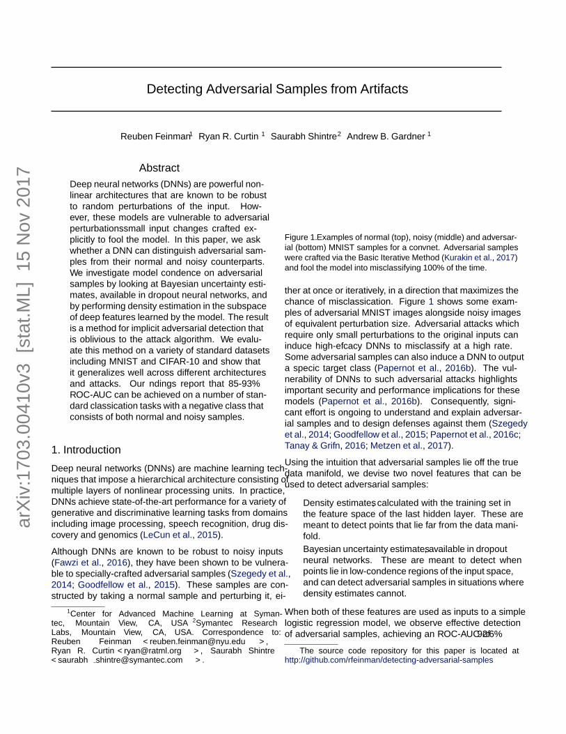
Figure 1. Examples of normal (top), noisy (middle) and adversar-ial (bottom) MNIST samples for a convnet. Adversarial sampleswere crafted via the Basic Iterative Method (Kurakin et al., 2017)and fool the model into misclassifying 100% of the time.

ther at once or iteratively, in a direction that maximizes thechance of misclassification. Figure 1 shows some exam-ples of adversarial MNIST images alongside noisy imagesof equivalent perturbation size. Adversarial attacks whichrequire only small perturbations to the original inputs caninduce high-efficacy DNNs to misclassify at a high rate.Some adversarial samples can also induce a DNN to outputa specific target class (Papernot et al., 2016b). The vul-nerability of DNNs to such adversarial attacks highlightsimportant security and performance implications for thesemodels (Papernot et al., 2016b). Consequently, signifi-cant effort is ongoing to understand and explain adversar-ial samples and to design defenses against them (Szegedyet al., 2014; Goodfellow et al., 2015; Papernot et al., 2016c;Tanay & Griffin, 2016; Metzen et al., 2017).

Using the intuition that adversarial samples lie off the truedata manifold, we devise two novel features that can beused to detect adversarial samples:

• Density estimates, calculated with the training set inthe feature space of the last hidden layer. These aremeant to detect points that lie far from the data mani-fold.

• Bayesian uncertainty estimates, available in dropoutneural networks. These are meant to detect whenpoints lie in low-confidence regions of the input space,and can detect adversarial samples in situations wheredensity estimates cannot.

When both of these features are used as inputs to a simplelogistic regression model, we observe effective detectionof adversarial samples, achieving an ROC-AUC of 92.6%

The source code repository for this paper is located athttp://github.com/rfeinman/detecting-adversarial-samples

arX

iv:1

703.

0041

0v3

[st

at.M

L]

15

Nov

201

7

Detecting Adversarial Samples from Artifacts

on the MNIST dataset with both noisy and normal samplesas the negative class. In Section 2 we provide the relevantbackground information for our approach, and in Section3 we briefly review a few state-of-the-art adversarial at-tacks. Then, we introduce the intuition for our approachin Section 4, with a discussion of manifolds and Bayesianuncertainty. This leads us to our results and conclusions inSections 5 and 6.

2. BackgroundWhile neural networks are known to be robust to randomnoise (Fawzi et al., 2016), they have been shown to bevulnerable to adversarially-crafted perturbations (Szegedyet al., 2014; Goodfellow et al., 2015; Papernot et al.,2016b). Specifically, an adversary can use informationabout the model to craft small perturbations that fool thenetwork into misclassifying their inputs. In the context ofobject classification, these perturbations are often imper-ceptible to the human eye, yet they can force the model tomisclassify with high model confidence.

A number of works have attempted to explain the vul-nerability of DNNs to adversarial samples. Szegedyet al. (2014) offered a simple preliminary explanation forthe phenomenon, arguing that low-probability adversarial“pockets” are densely distributed in input space. As a re-sult, they argued, every point in image space is close toa vast number of adversarial points and can be easily ma-nipulated to achieve a desired model outcome. Goodfel-low et al. (2015) argued that it is a result of the linear na-ture of deep classifiers. Although this explanation has beenthe most well-accepted in the field, it was recently weak-ened by counterexamples (Tanay & Griffin, 2016). Tanay& Griffin (2016) introduced the ‘boundary tilting’ perspec-tive, suggesting instead that adversarial samples lie in re-gions where the classification boundary is close to the man-ifold of training data.

Research in adversarial attack defense generally fallswithin two categories: first, methods for improving the ro-bustness of classifiers to current attacks, and second, meth-ods for detecting adversarial samples in the wild. Good-fellow et al. (2015) proposed augmenting the training lossfunction with an additional adversarial term to improvethe robustness of these models to a specific adversarial at-tack. Defensive distillation (Papernot et al., 2016c) is an-other recently-introduced technique which involves train-ing a DNN with the softmax outputs of another neural net-work that was trained on the training data, and can be seenas a way of preventing the network from fitting too tightlyto the data. Defensive distillation is effective against the at-tack of Papernot et al. (2016b). However, Carlini & Wagner(2016) showed that defensive distillation is easily brokenwith a modified attack.

On the detection of adversarial samples, Metzen et al.(2017) proposed augmenting a DNN with an additional“detector” subnetwork, trained on normal and adversarialsamples. Although the authors show compelling perfor-mance results on a number of state-of-the-art adversarialattacks, one major drawback is that the detector subnetworkmust be trained on generated adversarial samples. This im-plicitly trains the detector on a subset of all possible ad-versarial attacks; we do not know how comprehensive thissubset is, and future attack modifications may be able tosurmount the system. The robustness of this technique torandom noise is not currently known.

3. Adversarial AttacksThe typical goal of an adversary is to craft a sample thatlooks similar to a normal sample, and yet that gets misclas-sified by the target model. In the realm of image classi-fication, this amounts to finding a small perturbation that,when added to a normal image, causes the target model tomisclassify the sample, but remains correctly classified bythe human eye. For a given input image x, the goal is tofind a minimal perturbation η such that the adversarial in-put x = x+ η is misclassified. A significant number of ad-versarial attacks satisfying this goal have been introducedin recent years. This allows us a wide range of attacks tochoose from in our investigation. Here, we introduce someof the most well-known and most recent attacks.

Fast Gradient Sign Method (FGSM): Goodfellow et al.(2015) introduced the Fast Gradient Sign Method for craft-ing adversarial perturbations using the derivative of themodel’s loss function with respect to the input feature vec-tor. Given a base input, the approach is to perturb each fea-ture in the direction of the gradient by magnitude ε, whereε is a parameter that determines perturbation size. For amodel with loss J(Θ, x, y), where Θ represents the modelparameters, x is the model input, and y is the label of x, theadversarial sample is generated as

x∗ = x+ ε sign(∇xJ(Θ, x, y)).

With small ε, it is possible to fool DNNs trained for theMNIST and CIFAR-10 classification tasks with high suc-cess rate (Goodfellow et al., 2015).

Basic Iterative Method (BIM): Kurakin et al. (2017) pro-posed an iterative version of FGSM called the Basic Itera-tive Method. This is a straightforward extension; instead ofmerely applying adversarial noise η once with one param-eter ε, apply it many times iteratively with small ε. Thisgives a recursive formula:

x∗0 = x,

x∗i = clipx,ε(x∗i−1 + ε sign(∇x∗

i−1J(Θ, x∗i−1, y))).

Detecting Adversarial Samples from Artifacts

Here, clipx,ε(·) represents a clipping of the values ofthe adversarial sample such that they are within an ε-neighborhood of the original sample x. This approach isconvenient because it allows extra control over the attack.For instance, one can control how far past the classifica-tion boundary a sample is pushed: one can terminate theloop on the iteration when x∗i is first misclassified, or addadditional noise beyond that point.

The basic iterative method was shown to be typically moreeffective than the FGSM attack on ImageNet images (Ku-rakin et al., 2017).

Jacobian-based Saliency Map Attack (JSMA): Papernotet al. (2016b) proposed a simple iterative method for tar-geted misclassification. By exploiting the forward deriva-tive of a DNN, one can find an adversarial perturbation thatwill force the model to misclassify into a specific targetclass. For an input x and a neural network F , the outputfor class j is denoted Fj(x). To achieve a target class t,Ft(X) must be increased while the probabilities Fj(X) ofall other classes j 6= t decrease, until t = arg maxj Fj(X).This is accomplished by exploiting the adversarial saliencymap, which is defined as

S(X, t)[i] =

{0, if ∂Ft(X)

∂Xi< 0 or

∑j 6=t

∂Fj(X)∂Xi

> 0

(∂Ft(X)∂Xi

)|∑j 6=t

∂Fj(X)∂Xi

|, otherwise

for an input feature i. Starting with a normal samplex, we locate the pair of features {i, j} that maximizeS(X, t)[i] + S(X, t)[j], and perturb each feature by a con-stant offset ε. This process is repeated iteratively until thetarget misclassification is achieved. This method can effec-tively produce MNIST samples that are correctly classifiedby human subjects but misclassified into a specific targetclass by a DNN with high success rate.

Carlini & Wagner (C&W): Carlini & Wagner (2016) re-cently introduced a technique that is able to overcome de-fensive distillation. In fact, their technique encompassesa range of attacks, all cast through the same optimizationframework. This results in three powerful attacks, each fora different distance metric: an L2 attack, an L0 attack, andan L∞ attack. For the L0 attack, which we will considerin this paper, the perturbation δ is defined in terms of anauxiliary variable ω as

δ∗i =1

2(tanh(ωi + 1))− xi.

Then, to find δ∗ (an ‘unrestricted perturbation’), we opti-mize over ω:

minω

∥∥∥∥1

2(tanh(ω) + 1)− x

∥∥∥∥22

+ cf

(1

2tanh(ω) + 1

)

where f(·) is an objective function based on the hinge loss:

f(x) = max(max{Z(x)i : i 6= t} − Z(x)t,−κ).

Here, Z(x)i is the pre-softmax output for class i, t is thetarget class, and κ is a parameter that controls the confi-dence with which the misclassification occurs.

Finally, to produce the adversarial sample x∗ = x + δ,we convert the unrestricted perturbation δ∗ to a restrictedperturbation δ, in order to reduce the number of changedpixels. By calculating the gradient ∇f(x + δ∗), we mayidentify those pixels δ∗i with little importance (small gradi-ent values) and take δi = 0; otherwise, for larger gradientvalues we take δi = δ∗i . This allows an effective attack withfew modified pixels, thus helping keep the norm of δ low.

These three attacks were shown to be particularly effec-tive in comparison to other attacks against networks trainedwith defensive distillation, achieving adversarial samplegeneration success rates of 100% where other techniqueswere not able to top 1%.

4. Artifacts of Adversarial SamplesEach of these adversarial sample generation algorithms areable to change the predicted label of a point without chang-ing the underlying true label: humans will still correctlyclassify an adversarial sample, but models will not. Thiscan be understood from the perspective of the manifold oftraining data. Many high-dimensional datasets, such as im-ages, are believed to lie on a low-dimensional manifold(Lee & Verleysen, 2007). Gardner et al. (2015) recentlyshowed that by carefully traversing the data manifold, onecan change the underlying true label of an image. The intu-ition is that adversarial perturbations—which do not consti-tute meaningful changes to the input—must push samplesoff of the data manifold. Tanay & Griffin (2016) base theirinvestigation of adversarial samples on the assumption thatadversarial samples lie near class boundaries that are closeto the edge of a data submanifold. Similarly, Goodfellowet al. (2015) demonstrate that DNNs perform correctly onlynear the small manifold of training data. Therefore, webase our work here on the assumption that adversarial sam-ples do not lie on the data manifold.

If we accept that adversarial samples are points that wouldnot arise naturally, then we can assume that a technique togenerate adversarial samples will, from a source point xwith class cx, typically generate an adversarial sample x∗

that does not lie on the manifold and is classified incor-rectly as cx∗ . If x∗ lies off of the data manifold, we maysplit into three possible situations:

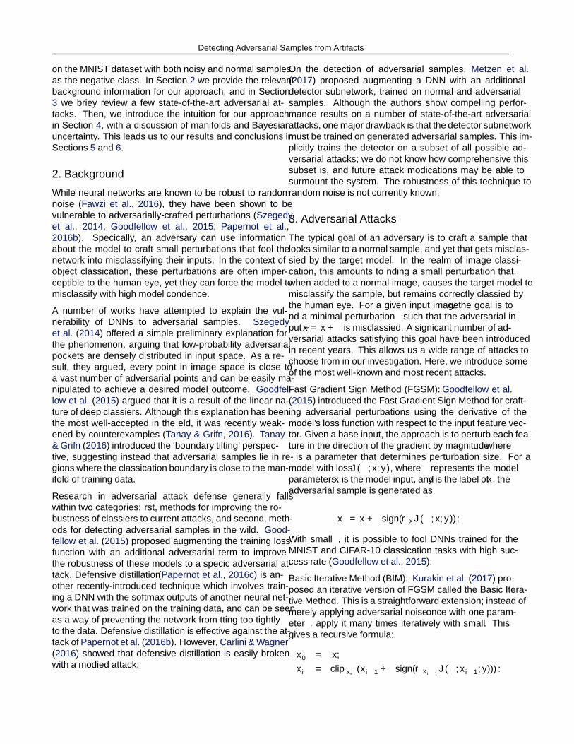
1. x∗ is far away from the submanifold of cx∗ .

Detecting Adversarial Samples from Artifacts

- +x

x∗

(a) Two simple 2D submanifolds.

-+

x

x∗

(b) One submanifold has a ‘pocket’.

-

+x

x∗

(c) Nearby 2D submanifolds.

Figure 2. (a): The adversarial sample x∗ is generated by moving off the ‘-’ submanifold and across the decision boundary (black dashedline), but x∗ still lies far from the ‘+’ submanifold. (b): the ‘+’ submanifold has a ‘pocket’, as in Szegedy et al. (2014). x∗ lies inthe pocket, presenting significant difficulty for detection. (c): the adversarial sample x∗ is near both the decision boundary and bothsubmanifolds.

2. x∗ is near the submanifold cx∗ but not on it, and x∗ isfar from the classification boundary separating classescx and cx∗ .

3. x∗ is near the submanifold cx∗ but not on it, and x∗ isnear the classification boundary separating classes cxand cx∗ .

Figures 2a through 2c show simplified example illustra-tions for each of these three situations in a two-dimensionalbinary classification setting.

4.1. Density Estimation

If we have an estimate of what the submanifold correspond-ing to data with class cx∗ is, then we can determine whetherx∗ falls near this submanifold after observing the predic-tion cx∗ . Following the intuition of Gardner et al. (2015)and hypotheses of Bengio et al. (2013), the deeper layersof a DNN provide more linear and ‘unwrapped’ manifoldsto work with than input space; therefore, we may use thisidea to model the submanifolds of each class by perform-ing kernel density estimation in the feature space of the lasthidden layer.

The standard technique of kernel density estimation can,given the point x and the set Xt of training points withlabel t, provide a density estimate f(x) that can be usedas a measure of how far x is from the submanifold for t.Specifically,

f(x) =1

|Xt|∑xi∈Xt

k(xi, x) (1)

where k(·, ·) is the kernel function, often chosen as a Gaus-sian with bandwidth σ:

kσ(x, y) ∼ exp(−‖x− y‖2/σ2). (2)

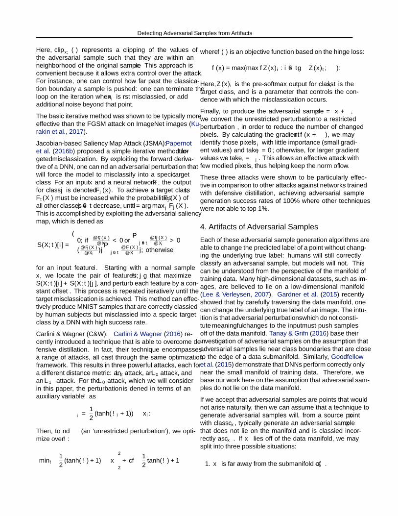
The bandwidth may typically be chosen as a value that

maximizes the log-likelihood of the training data (Joneset al., 1996). A value too small will give rise to a ‘spiky’density estimate with too many gaps (see Figure 3), but avalue too large will give rise to an overly-smooth densityestimate (see Figure 4). This also implies that the estimateis improved as the training set size |Xt| increases, sincewe are able to use smaller bandwidths without the estimatebecoming too ‘spiky.’

For the manifold estimate, we operate in the space of thelast hidden layer. This layer provides a space of reasonabledimensionality in which we expect the manifold of our datato be simplified. If φ(x) is the last hidden layer activationvector for point x, then our density estimate for a point xwith predicted class t is defined as

K(x,Xt) =∑xi∈Xt

kσ(φ(x), φ(xi)) (3)

whereXt is the set of training points of class t, and σ is thetuned bandwidth.

To validate our intuition about the utility of this density es-timate, we perform a toy experiment using the BIM attackwith a convnet trained on MNIST data. In Figure 5, we

Figure 3. ‘spiky’ density estimate from a too-small bandwidth on1-D points sampled from a bimodal distribution.

Figure 4. Overly smooth density estimate from a too-large band-width on 1-D points sampled from a bimodal distribution.

Detecting Adversarial Samples from Artifacts

iteration

K

iteration

K

iteration

K

iteration

K

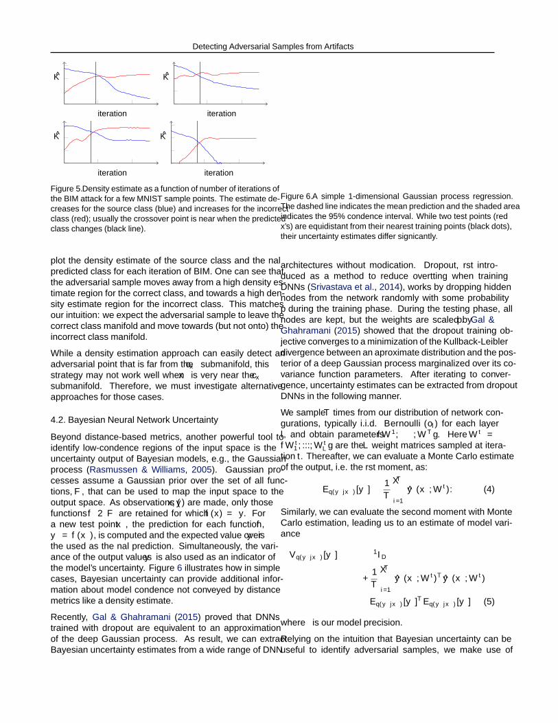
Figure 5. Density estimate as a function of number of iterations ofthe BIM attack for a few MNIST sample points. The estimate de-creases for the source class (blue) and increases for the incorrectclass (red); usually the crossover point is near when the predictedclass changes (black line).

plot the density estimate of the source class and the finalpredicted class for each iteration of BIM. One can see thatthe adversarial sample moves away from a high density es-timate region for the correct class, and towards a high den-sity estimate region for the incorrect class. This matchesour intuition: we expect the adversarial sample to leave thecorrect class manifold and move towards (but not onto) theincorrect class manifold.

While a density estimation approach can easily detect anadversarial point that is far from the cx∗ submanifold, thisstrategy may not work well when x∗ is very near the cx∗

submanifold. Therefore, we must investigate alternativeapproaches for those cases.

4.2. Bayesian Neural Network Uncertainty

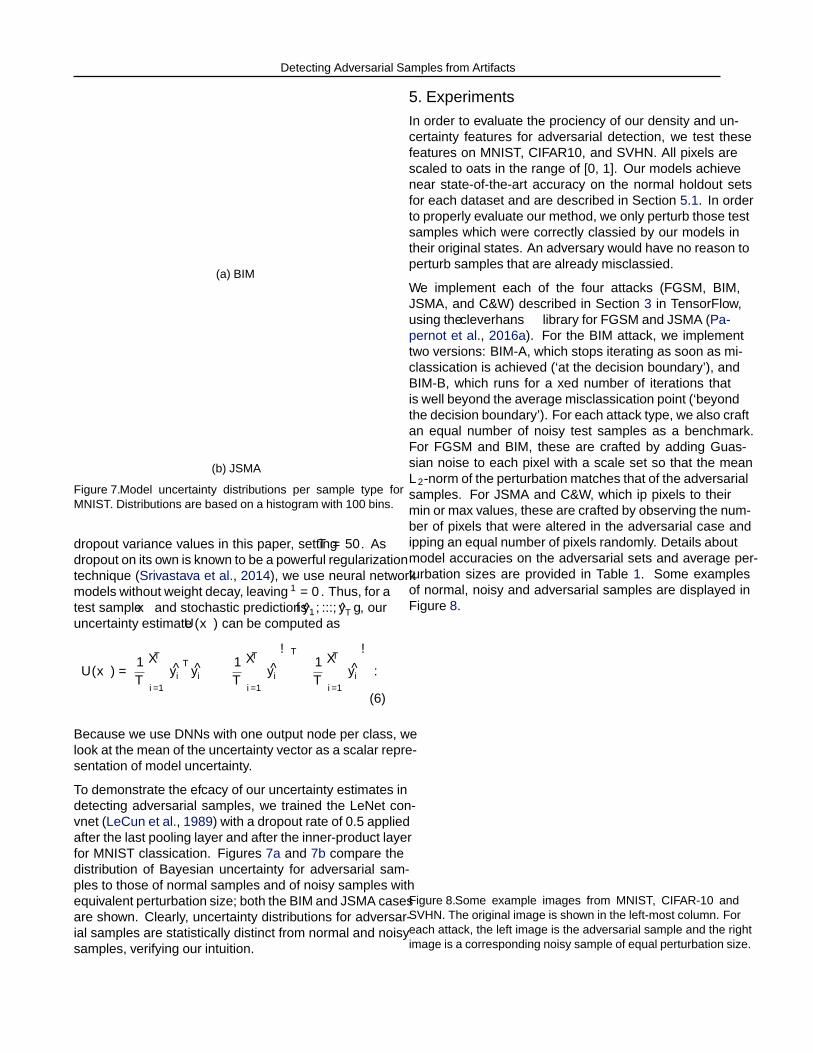
Beyond distance-based metrics, another powerful tool toidentify low-confidence regions of the input space is theuncertainty output of Bayesian models, e.g., the Gaussianprocess (Rasmussen & Williams, 2005). Gaussian pro-cesses assume a Gaussian prior over the set of all func-tions, F , that can be used to map the input space to theoutput space. As observations (x, y) are made, only thosefunctions f ∈ F are retained for which f(x) = y. Fora new test point x∗, the prediction for each function f ,y∗ = f(x∗), is computed and the expected value over y∗ isthe used as the final prediction. Simultaneously, the vari-ance of the output values y∗ is also used as an indicator ofthe model’s uncertainty. Figure 6 illustrates how in simplecases, Bayesian uncertainty can provide additional infor-mation about model confidence not conveyed by distancemetrics like a density estimate.

Recently, Gal & Ghahramani (2015) proved that DNNstrained with dropout are equivalent to an approximationof the deep Gaussian process. As result, we can extractBayesian uncertainty estimates from a wide range of DNN

Figure 6. A simple 1-dimensional Gaussian process regression.The dashed line indicates the mean prediction and the shaded areaindicates the 95% confidence interval. While two test points (redx’s) are equidistant from their nearest training points (black dots),their uncertainty estimates differ significantly.

architectures without modification. Dropout, first intro-duced as a method to reduce overfitting when trainingDNNs (Srivastava et al., 2014), works by dropping hiddennodes from the network randomly with some probabilityp during the training phase. During the testing phase, allnodes are kept, but the weights are scaled by p. Gal &Ghahramani (2015) showed that the dropout training ob-jective converges to a minimization of the Kullback-Leiblerdivergence between an aproximate distribution and the pos-terior of a deep Gaussian process marginalized over its co-variance function parameters. After iterating to conver-gence, uncertainty estimates can be extracted from dropoutDNNs in the following manner.

We sample T times from our distribution of network con-figurations, typically i.i.d. Bernoulli(ol) for each layerl, and obtain parameters {W 1, · · · ,WT }. Here W t ={W t

1 , ...,WtL} are the L weight matrices sampled at itera-

tion t. Thereafter, we can evaluate a Monte Carlo estimateof the output, i.e. the first moment, as:

Eq(y∗|x∗)[y∗] ≈ 1

T

T∑i=1

y∗(x∗,W t). (4)

Similarly, we can evaluate the second moment with MonteCarlo estimation, leading us to an estimate of model vari-ance

Vq(y∗|x∗)[y∗] ≈ τ−1ID

+1

T

T∑i=1

y∗(x∗,W t)T y∗(x∗,W t)

−Eq(y∗|x∗)[y∗]TEq(y∗|x∗)[y

∗] (5)

where τ is our model precision.

Relying on the intuition that Bayesian uncertainty can beuseful to identify adversarial samples, we make use of

Detecting Adversarial Samples from Artifacts

(a) BIM

(b) JSMA

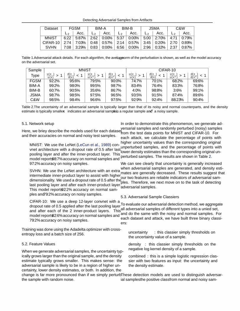
Figure 7. Model uncertainty distributions per sample type forMNIST. Distributions are based on a histogram with 100 bins.

dropout variance values in this paper, setting T = 50. Asdropout on its own is known to be a powerful regularizationtechnique (Srivastava et al., 2014), we use neural networkmodels without weight decay, leaving τ−1 = 0. Thus, for atest sample x∗ and stochastic predictions {y∗1 , ..., y∗T }, ouruncertainty estimate U(x∗) can be computed as

U(x∗) =1

T

T∑i=1

y∗iTy∗i −

(1

T

T∑i=1

y∗i

)T (1

T

T∑i=1

y∗i

).

(6)

Because we use DNNs with one output node per class, welook at the mean of the uncertainty vector as a scalar repre-sentation of model uncertainty.

To demonstrate the efficacy of our uncertainty estimates indetecting adversarial samples, we trained the LeNet con-vnet (LeCun et al., 1989) with a dropout rate of 0.5 appliedafter the last pooling layer and after the inner-product layerfor MNIST classification. Figures 7a and 7b compare thedistribution of Bayesian uncertainty for adversarial sam-ples to those of normal samples and of noisy samples withequivalent perturbation size; both the BIM and JSMA casesare shown. Clearly, uncertainty distributions for adversar-ial samples are statistically distinct from normal and noisysamples, verifying our intuition.

5. ExperimentsIn order to evaluate the proficiency of our density and un-certainty features for adversarial detection, we test thesefeatures on MNIST, CIFAR10, and SVHN. All pixels arescaled to floats in the range of [0, 1]. Our models achievenear state-of-the-art accuracy on the normal holdout setsfor each dataset and are described in Section 5.1. In orderto properly evaluate our method, we only perturb those testsamples which were correctly classified by our models intheir original states. An adversary would have no reason toperturb samples that are already misclassified.

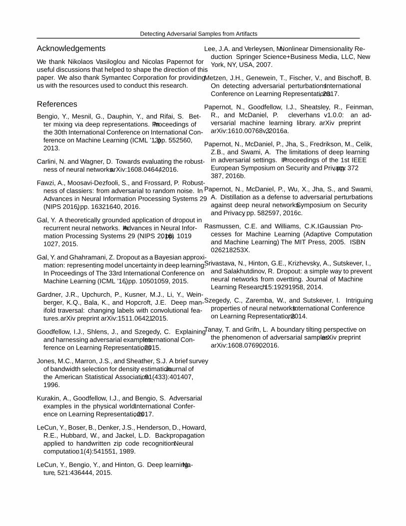
We implement each of the four attacks (FGSM, BIM,JSMA, and C&W) described in Section 3 in TensorFlow,using the cleverhans library for FGSM and JSMA (Pa-pernot et al., 2016a). For the BIM attack, we implementtwo versions: BIM-A, which stops iterating as soon as mi-classification is achieved (‘at the decision boundary’), andBIM-B, which runs for a fixed number of iterations thatis well beyond the average misclassification point (‘beyondthe decision boundary’). For each attack type, we also craftan equal number of noisy test samples as a benchmark.For FGSM and BIM, these are crafted by adding Guas-sian noise to each pixel with a scale set so that the meanL2-norm of the perturbation matches that of the adversarialsamples. For JSMA and C&W, which flip pixels to theirmin or max values, these are crafted by observing the num-ber of pixels that were altered in the adversarial case andflipping an equal number of pixels randomly. Details aboutmodel accuracies on the adversarial sets and average per-turbation sizes are provided in Table 1. Some examplesof normal, noisy and adversarial samples are displayed inFigure 8.

Figure 8. Some example images from MNIST, CIFAR-10 andSVHN. The original image is shown in the left-most column. Foreach attack, the left image is the adversarial sample and the rightimage is a corresponding noisy sample of equal perturbation size.

Detecting Adversarial Samples from Artifacts

Dataset FGSM BIM-A BIM-B JSMA C&WL2 Acc. L2 Acc. L2 Acc. L2 Acc. L2 Acc.

MNIST 6.22 5.87% 2.62 0.00% 5.37 0.00% 5.00 2.70% 4.71 0.79%CIFAR-10 2.74 7.03% 0.48 0.57% 2.14 0.57% 3.45 0.20% 2.70 0.89%

SVHN 7.08 3.29% 0.83 0.00% 6.56 0.00% 2.96 0.32% 2.37 0.87%

Table 1. Adversarial attack details. For each algorithm, the average L2-norm of the perturbation is shown, as well as the model accuracyon the adversarial set.

Sample MNIST CIFAR-10Type u(x∗)

u(x) > 1 d(x∗)d(x) < 1 u(x∗)

u(xn) > 1 d(x∗)d(xn) < 1 u(x∗)

u(x) > 1 d(x∗)d(x) < 1 u(x∗)

u(xn) > 1 d(x∗)d(xn) < 1

FGSM 92.2% 95.6% 79.5% 90.0% 74.7% 70.1% 68.2% 69.6%BIM-A 99.2% 98.0% 99.5% 98.7% 83.4% 76.4% 83.3% 76.8%BIM-B 60.7% 90.5% 35.6% 86.7% 4.0% 98.8% 3.6% 99.1%JSMA 98.7% 98.5% 97.5% 96.5% 93.5% 91.5% 87.4% 89.6%C&W 98.5% 98.4% 96.6% 97.5% 92.9% 92.4% 88.23% 90.4%

Table 2. The uncertainty of an adversarial sample is typically larger than that of its noisy and normal counterparts, and the densityestimate is typically smaller. x∗ indicates an adversarial sample, x is a regular sample and xn a noisy sample.

5.1. Network setup

Here, we briefly describe the models used for each datasetand their accuracies on normal and noisy test samples.

• MNIST: We use the LeNet (LeCun et al., 1989) con-vnet architecture with a dropout rate of 0.5 after lastpooling layer and after the inner-product layer. Thismodel reports 98.7% accuracy on normal samples and97.2% accuracy on noisy samples.

• SVHN: We use the LeNet architecture with an extraintermediate inner-product layer to assist with higherdimensionality. We used a dropout rate of 0.5 after thelast pooling layer and after each inner-product layer.This model reports 92.2% accuracy on normal sam-ples and 79.2% accuracy on noisy samples.

• CIFAR-10: We use a deep 12-layer convnet with adropout rate of 0.5 applied after the last pooling layerand after each of the 2 inner-product layers. Thismodel reports 82.6% accuracy on normal samples and79.2% accuracy on noisy samples.

Training was done using the Adadelta optimizer with cross-entropy loss and a batch size of 256.

5.2. Feature Values

When we generate adversarial samples, the uncertainty typ-ically grows larger than the original sample, and the densityestimate typically grows smaller. This makes sense: theadversarial sample is likely to be in a region of higher un-certainty, lower density estimates, or both. In addition, thechange is far more pronounced than if we simply perturbthe sample with random noise.

In order to demonstrate this phenomenon, we generate ad-versarial samples and randomly perturbed (noisy) samplesfrom the test data points for MNIST and CIFAR-10. Foreach attack, we calculate the percentage of points withhigher uncertainty values than the corresponding originalunperturbed samples, and the percentage of points withlower density estimates than the corresponding original un-perturbed samples. The results are shown in Table 2.

We can see clearly that uncertainty is generally increasedwhen adversarial samples are generated, and density esti-mates are generally decreased. These results suggest thatour two features are reliable indicators of adversarial sam-ples. Therefore, we next move on to the task of detectingadversarial samples.

5.3. Adversarial Sample Classifiers

To evaluate our adversarial detection method, we aggregateall adversarial samples of different types into a unified set,and do the same with the noisy and normal samples. Foreach dataset and attack, we have built three binary classi-fiers:

• uncertainty: this classifier simply thresholds onthe uncertainty value of a sample.

• density: this classifier simply thresholds on thenegative log kernel density of a sample.

• combined: this is a simple logistic regression clas-sifier with two features as input: the uncertainty andthe density estimate.

These detection models are used to distinguish adversar-ial samples–the positive class–from normal and noisy sam-

Detecting Adversarial Samples from Artifacts

Dataset FGSM BIM-A BIM-B JSMA C&W OverallMNIST 90.57% 97.23% 82.06% 98.13% 97.94% 92.59%

CIFAR-10 72.23% 81.05% 95.41% 91.52% 92.17% 85.54%SVHN 89.04% 82.12% 99.91% 91.34% 92.82% 90.20%

Table 3. ROC-AUC measures for each dataset and each attack for the logistic regression classifier (combined).

(a) MNIST dataset. (b) SVHN dataset. (c) CIFAR-10 dataset.

Figure 9. ROCS for the different classifier types. The blue line indicates uncertainty, green line density, and red line combined.The negative class consists of both normal and noisy samples.

ples, which jointly constitue the negative class. The logisticregression model is trained by generating adversarial sam-ples for every correctly-classified training point using eachof the four adversarial attacks, and then using the uncer-tainty values and density estimates for the original and ad-versarial samples as a labeled training set. The two featuresare z-scored before training.

Because these are all threshold-based classifiers, we maygenerate an ROC for each method. Figure 9 shows ROCsfor each classifier with a couple of datasets. We see that theperformance of the combined classifier is better than ei-ther the uncertainty or density classifiers, demon-strating that each feature is able to detect different qualitiesof adversarial features. Further, the ROCs demonstrate thatthe uncertainty and density estimates are effective indica-tors that can be used to detect if a sample is adversarial.

Figure 10. ROC results per adversarial attack for combined clas-sifier on MNIST.

Figure 10 shows the ROCs for each individual attack; thecombined classifier is able to most easily handle the JSMA,BIM-A and C&W attacks.

In Table 3, the ROC-AUC measures are shown, for each ofthe three classifiers, on each dataset, for each attack. Theperformance is quite good, suggesting that the combinedclassifier is able to effectively detect adversarial samplesfrom a wide range of attacks on a wide range of datasets.

6. ConclusionsWe have shown that adversarial samples crafted to foolDNNs can be effectively detected with two new features:kernel density estimates in the subspace of the last hiddenlayer, and Bayesian neural network uncertainty estimates.These two features handle complementary situations, andcan be combined as an effective defense mechanism againstadversarial samples. Our results report that we can, in somecases, obtain an ROC-AUC for an adversarial sample de-tector of up to 90% or more when both normal and noisysamples constitute the negative class. The performance isgood on a wide variety of attacks and a range of imagedatasets.

In our work here, we have only considered convolutionalneural networks. However, we believe that this approachcan be extended to other neural network architectures aswell. Gal (2015) showed that the idea of dropout as aBayesian approximation could be applied to RNNs as well,allowing for robust uncertainty estimation. In future work,we aim to apply our features to RNNs and other networkarchitectures.

Detecting Adversarial Samples from Artifacts

AcknowledgementsWe thank Nikolaos Vasiloglou and Nicolas Papernot foruseful discussions that helped to shape the direction of thispaper. We also thank Symantec Corporation for providingus with the resources used to conduct this research.

ReferencesBengio, Y., Mesnil, G., Dauphin, Y., and Rifai, S. Bet-

ter mixing via deep representations. In Proceedings ofthe 30th International Conference on International Con-ference on Machine Learning (ICML ’13), pp. 552–560,2013.

Carlini, N. and Wagner, D. Towards evaluating the robust-ness of neural networks. arXiv:1608.04644, 2016.

Fawzi, A., Moosavi-Dezfooli, S., and Frossard, P. Robust-ness of classifiers: from adversarial to random noise. InAdvances in Neural Information Processing Systems 29(NIPS 2016), pp. 1632–1640, 2016.

Gal, Y. A theoretically grounded application of dropout inrecurrent neural networks. In Advances in Neural Infor-mation Processing Systems 29 (NIPS 2016), pp. 1019–1027, 2015.

Gal, Y. and Ghahramani, Z. Dropout as a Bayesian approxi-mation: representing model uncertainty in deep learning.In Proceedings of The 33rd International Conference onMachine Learning (ICML ’16), pp. 1050–1059, 2015.

Gardner, J.R., Upchurch, P., Kusner, M.J., Li, Y., Wein-berger, K.Q., Bala, K., and Hopcroft, J.E. Deep man-ifold traversal: changing labels with convolutional fea-tures. arXiv preprint arXiv:1511.06421, 2015.

Goodfellow, I.J., Shlens, J., and Szegedy, C. Explainingand harnessing adversarial examples. International Con-ference on Learning Representations, 2015.

Jones, M.C., Marron, J.S., and Sheather, S.J. A brief surveyof bandwidth selection for density estimation. Journal ofthe American Statistical Association, 91(433):401–407,1996.

Kurakin, A., Goodfellow, I.J., and Bengio, S. Adversarialexamples in the physical world. International Confer-ence on Learning Representations, 2017.

LeCun, Y., Boser, B., Denker, J.S., Henderson, D., Howard,R.E., Hubbard, W., and Jackel, L.D. Backpropagationapplied to handwritten zip code recognition. Neuralcomputation, 1(4):541–551, 1989.

LeCun, Y., Bengio, Y., and Hinton, G. Deep learning. Na-ture, 521:436–444, 2015.

Lee, J.A. and Verleysen, M. Nonlinear Dimensionality Re-duction. Springer Science+Business Media, LLC, NewYork, NY, USA, 2007.

Metzen, J.H., Genewein, T., Fischer, V., and Bischoff, B.On detecting adversarial perturbations. InternationalConference on Learning Representations, 2017.

Papernot, N., Goodfellow, I.J., Sheatsley, R., Feinman,R., and McDaniel, P. cleverhans v1.0.0: an ad-versarial machine learning library. arXiv preprintarXiv:1610.00768v3, 2016a.

Papernot, N., McDaniel, P., Jha, S., Fredrikson, M., Celik,Z.B., and Swami, A. The limitations of deep learningin adversarial settings. In Proceedings of the 1st IEEEEuropean Symposium on Security and Privacy, pp. 372–387, 2016b.

Papernot, N., McDaniel, P., Wu, X., Jha, S., and Swami,A. Distillation as a defense to adversarial perturbationsagainst deep neural networks. Symposium on Securityand Privacy, pp. 582–597, 2016c.

Rasmussen, C.E. and Williams, C.K.I. Gaussian Pro-cesses for Machine Learning (Adaptive Computationand Machine Learning). The MIT Press, 2005. ISBN026218253X.

Srivastava, N., Hinton, G.E., Krizhevsky, A., Sutskever, I.,and Salakhutdinov, R. Dropout: a simple way to preventneural networks from overfitting. Journal of MachineLearning Research, 15:1929–1958, 2014.

Szegedy, C., Zaremba, W., and Sutskever, I. Intriguingproperties of neural networks. International Conferenceon Learning Representations, 2014.

Tanay, T. and Griffin, L. A boundary tilting perspective onthe phenomenon of adversarial samples. arXiv preprintarXiv:1608.07690, 2016.