Detailed Formulation and Programming Method for ... · PDF fileA special purpose MATLAB code...
21
Int. J. Pure Appl. Sci. Technol., 7(1) (2011), pp.1-21 International Journal of Pure and Applied Sciences and Technology ISSN 2229 - 6107 Available online at www.ijopaasat.in Research Paper Detailed Formulation and Programming Method for Piezoelectric Finite Element Chandrashekhar Bendigeri 1,* , Ritu Tomar 2 , Basavaraju S 3 and Arasukumar K 4 1 Department of Mechanical Engineering , UVCE, Bangalore University, Bangalore-560 001, India 2 Department of Physics, Research Center, Sambhram Institute of Technology Bangalore-560 097, India 3 Atria Institute of Technology, Anandnagar, Bangalore - 560 024, India 4 Rajiv Gandhi Institute of Technology, Cholanagar, R.T. Nagar post, Bangalore - 560 032, India . *Corresponding author, e-mail: ([email protected]) (Received: 10-3-11; Accepted: 14-9-11) Abstract: The scope of the present investigation encompasses the use of property of piezoelectric material in modeling the sensing and actuation of smart composite hexahedral element. The finite element is developed for the static and dynamic analysis of a smart structure. An eight noded, isoparametric three dimensional hexahedral element is developed to model the coupled electro-mechanical behavior. The formulation of the present research work accounts for the effects due to piezoelectric for the developed finite element. The mechanical stress, electric displacement is related to mechanical strains and electric potential. As a result, one obtains governing equations that are coupled. The coupled governing equations are solved using finite element method. An eight noded hexahedral finite element having three mechanical displacements and one electric potential as degrees of freedom at each node is developed. A special purpose MATLAB code is developed based on the formulation considered in the present work. Keywords: piezoelectric, finite element, electromechanical, sensing and actuation 1. Introduction Recent advances in the field of distributed sensing and actuation have led to the development of new structures called smart structures. A smart/Intelligent structure is able to sense or respond and control its own characteristics and state. A structure becomes smart when the load bearing, also called substrate is composed of conventional structural material and is integrated with distributed actuator/sensor to achieve self controlling and self monitoring capabilities. Among the entire smart materials, piezoelectric have gained popularity both as sensors and actuators. The study of piezoelectric composite structures involves structural and electromechanical analysis.
-
Upload
truonghuong -
Category
Documents
-
view
218 -
download
1
Transcript of Detailed Formulation and Programming Method for ... · PDF fileA special purpose MATLAB code...
Int. J. Pure Appl. Sci. Technol., 7(1) (2011), pp.1-21
International Journal of Pure and Applied Sciences and Technology ISSN 2229 - 6107 Available online at www.ijopaasat.in
Research Paper
Detailed Formulation and Programming Method for Piezoelectric Finite Element Chandrashekhar Bendigeri1,*, Ritu Tomar2 , Basavaraju S3 and Arasukumar K4 1Department of Mechanical Engineering , UVCE, Bangalore University, Bangalore-560 001, India
2 Department of Physics, Research Center, Sambhram Institute of Technology Bangalore-560 097, India
3 Atria Institute of Technology, Anandnagar, Bangalore - 560 024, India 4 Rajiv Gandhi Institute of Technology, Cholanagar, R.T. Nagar post, Bangalore - 560 032, India . *Corresponding author, e-mail: ([email protected])
(Received: 10-3-11; Accepted: 14-9-11)
Abstract: The scope of the present investigation encompasses the use of property of piezoelectric material in modeling the sensing and actuation of smart composite hexahedral element. The finite element is developed for the static and dynamic analysis of a smart structure. An eight noded, isoparametric three dimensional hexahedral element is developed to model the coupled electro-mechanical behavior. The formulation of the present research work accounts for the effects due to piezoelectric for the developed finite element. The mechanical stress, electric displacement is related to mechanical strains and electric potential. As a result, one obtains governing equations that are coupled. The coupled governing equations are solved using finite element method. An eight noded hexahedral finite element having three mechanical displacements and one electric potential as degrees of freedom at each node is developed. A special purpose MATLAB code is developed based on the formulation considered in the present work. Keywords: piezoelectric, finite element, electromechanical, sensing and actuation
1. Introduction Recent advances in the field of distributed sensing and actuation have led to the development of new structures called smart structures. A smart/Intelligent structure is able to sense or respond and control its own characteristics and state. A structure becomes smart when the load bearing, also called substrate is composed of conventional structural material and is integrated with distributed actuator/sensor to achieve self controlling and self monitoring capabilities. Among the entire smart materials, piezoelectric have gained popularity both as sensors and actuators. The study of piezoelectric composite structures involves structural and electromechanical analysis.

Int. J. Pure Appl. Sci. Technol., 7(1) (2011), 1-21. 2
2. Piezoelectricity Piezoelectricity from the Greek word "piezo" means pressure electricity. It is the property of certain crystalline substances to generate electrical charges on the application of mechanical stress. Conversely, if the crystal is placed in an electric field, it will experience a mechanical strain. The first property makes them suitable as sensors, whereas the second property makes them suitable as actuators to control structural response. Thus piezoelectric materials have the property to into mechanical energy and vice versa. When an AC voltage is applied, it will cause it to vibrate and thus generate mechanical waves at the same frequency of the input AC field. Similarly, it would sense the input mechanical vibrations and produce the proportional charge at the matching frequency of the mechanical input. 3. Piezoelectric finite element analysis The finite element method is being widely used numerical solution. Chien-Chang Lin [1] presented basic equation of piezo sensor and actuator. The equation of motion for beam – plate structure bonded with pairs of piezoelectric sensors or actuator is derived using Hamilton principle. FEM was used, a control algorithm based on Lyapunov energy function was studied, and numerical results are presented. Chang Ho Hong et al [2] formulated a consistent plate finite element model for coupled composite plated with induced strain actuation and validated with test data obtained from cantilever isotropic and anisotropic plates. Ho-Jun Lee et al [3] formulated coupled mechanical, electrical and thermal response. A robust layerwise theory is formulated with the inherent capability to explicitly model the active and sensory response of piezoelectric composite plates having general limitation in thermal environment. Gim [4] has developed a plate finite element based on lamination theory that includes the effect of transverse shear deformation. To ensure compatibility and equilibrium of resultant forces and moments at the delamination crack tip, a multipoint constraint algorithm has been developed and incorporated into the finite element code. This study focuses on the development of an effective and adequate finite element routine based on shear deformable lamination theory. A structure (shell/plate) containing an integrated distributed piezoelectric sensor and actuator is proposed by Tzou et al [5]. A piezoelectric finite element with internal degrees of freedom is derived. The performance of a plate model with distributed piezoelectric sensor/actuators is evaluated applications to distributed dynamic measurement and controls of the advanced structures are also demonstrated. Finite element modeling for active –passive vibration damping was attempted by Trindade et al [6]. In part I the multilayer sandwich beams consisted of a viscoelastic core sandwiched between layered piezoelectric faces was modeled assuming Euler–Bernoulli thin faces and a Timoshenko thick core. The frequency dependency of the viscoelastic is handled through the anelastic displacement fields. In part II it was validated by performance analysis of a cantilever beam. Similar ideas was also proposed by Aditi Chattopadhyay for plates[7] Akpan et al developed a fuzzy finite element based approach for modeling smart structures with vague or imprecise uncertainties. Fuzzy sets are used to represent the uncertainties present in the piezoelectric, mechanical, thermal and physical properties of the smart structures[8]. J. Lopez-Bonilla has discussed Lanczos Derivative via a Quadrature Method[9]. Sung Kyu and Charles Keillers presented a finite element formulation for modeling the dynamic as well as static response of laminated composites. Experiments were also conducted to verify the analysis and the computer simulations[10].

Int. J. Pure Appl. Sci. Technol., 7(1) (2011), 1-21. 3
4. Finite element formulation 4.1 Introduction The finite element formulation for developing the finite element for structural and electromechanical analysis of piezoelectric composite structures have been presented in this chapter and also the features of present element and implementation on MATLAB have been explained. Also the stress calculation and Gauss Quadrature numerical integration that are used in the finite element code are explained. Flowchart1 contains details regarding the finite element method, which is the basis of present the finite element formulation, and its coding has been done using MATLAB software. 4.2 Element Formulation The formulation of the present finite element for structural and electromechanical analysis is explained as follows The governing equations for the electro-mechanical coupled system are based on classical, linear, 3–D piezoelectricity. 4.2.1 Assumptions The formulation of the present element is based on following assumptions I. Mechanical and electrical quantities are sufficiently small so that linear theories of
piezoelectricity are applicable. II. Magnetic effects are taken to be negligible as compared to electrical effects. The
variations due to temperature are also neglected. III. Perfect bonding occurs between the layers of the structure, including the
piezoelement and the base structure. IV. Electric field is quasi-static. V. The equations of linear elasticity are coupled to the charge equation of
electrostatics by means of piezoelectric constant. VI. The constitutive equation is the source of electrical and mechanical interactions. 4.2.2 Governing Equations of piezoelectricity Piezoelectric materials are anisotropy and the electric field in such materials is coupled with the mechanical stress and Vice-versa. The actuation of the piezoelectric material is obtained by applying voltage, which is known as converse coupling or actuator technique, and when mechanical load is applied voltage generated is sensed, which is known as direct coupling or sensor technique. Also constitutive relations are the relations expressing coupling between mechanical and electrical field .These constitutive relations are as follows
{ } [ ]{ } [ ]{ }EdC −= εσ (Converse coupling; actuator technique) (1)
{ } { } { } [ ]{ }EbdD T += ε (Direct coupling; sensor technique) (2)
Int. J. Pure Appl. Sci. Technol., 7(1) (2011), 1-21. 4
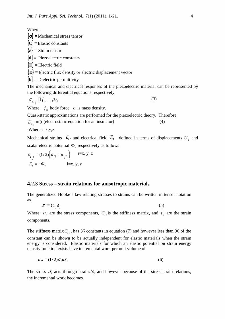
Where,
{ } =σσσσ Mechanical stress tensor
[ ] =C Elastic constants
{ } =εεεε Strain tensor
[ ] =d Piezoelectric constants
{ } =E Electric field
{ } =D Electric flux density or electric displacement vector
[ ] =b Dielectric permittivity
The mechanical and electrical responses of the piezoelectric material can be represented by the following differential equations respectively.
iibjij uf ρσ =+ (3)
Where ibf body force, ρ is mass density.
Quasi-static approximations are performed for the piezoelectric theory. Therefore,
0, =iiD (electrostatic equation for an insulator) (4)
Where i=x,y,z
Mechanical strains IJε and electrical field IE defined in terms of displacements jU and
scalar electric potential Φ , respectively as follows
+=
jiu
iju
ji)2/1(ε i=x, y, z
iiE Φ−= i=x, y, z
4.2.3 Stress – strain relations for anisotropic materials The generalized Hooke’s law relating stresses to strains can be written in tensor notation as jjii C εσ = (5)
Where, iσ are the stress components, jiC is the stiffness matrix, and jε are the strain
components. The stiffness matrix jiC , has 36 constants in equation (7) and however less than 36 of the
constant can be shown to be actually independent for elastic materials when the strain energy is considered. Elastic materials for which an elastic potential on strain energy density function exists have incremental work per unit volume of iiddw εσ)2/1(= (6)
The stress iσ acts through strain idε and however because of the stress-strain relations,
the incremental work becomes

Int. J. Pure Appl. Sci. Technol., 7(1) (2011), 1-21. 5
))(2/1( ijji dCdw εε=
Upon integration for all strains, the work per unit of volume is ))(2/1( jijiCw εε=
jjii Cw εε =∂∂ /
Where upon jiji Cw =∂∂ εε/2
Similarly
ijij Cw =∂∂∂ εε/2
But the order of differentiation of w is immaterial, so
ijji CC =
Thus the stiffness matrix is symmetrical. So only 21of the constants are independent. With the foregoing reduction from 36 to 21 independent constants, the stress-strain relations are
=
12
31
23
33
22
11
666564636261
565554535251
464544434241
363534333231
262524232221
161514131211
12
31
32
33
22
11
τττεεε
τττσσσ
CCCCCC
CCCCCC
CCCCCC
CCCCCC
CCCCCC
CCCCCC
(7)
The relations in equations (7) are referred to characterizing anisotropic materials since there are no planes of symmetry for the material properties. If there are two orthogonal planes of material symmetry for a material, symmetry will exist relative to a third mutually orthogonal plane. The stress – strain relations in co-ordinates aligned with principle material directions are
=
12
31
23
33
22
11
66
55
44
333231
232221
131211
12
31
32
33
22
11
00000
00000
00000
000
000
000
τττεεε
τττσσσ
C
C
C
CCC
CCC
CCC
(8)
The above stress – strain relations refer to an orthotropic material.

Int. J. Pure Appl. Sci. Technol., 7(1) (2011), 1-21. 6
4.2.4 Engineering constants for orthotropic materials
Engineering constants are generalized young’s modulus Poisson’s ratios, and shear modulli as well as other behavioral constants. These constants are measured in simple tests such as uniaxial tension or pure shear tests. Most simple test is performed with a known load on stress. The resulting displacement and then strain is measured. Thus, the components of compliance ( )ijS matrix are determined more directly than those of the
stiffness ( )ijC matrix, for an orthotropic material. The compliance matrix components in
terms of the engineering constants are
[ ]
−−−−−−
=
)/1(00000
0)/1(0000
00)/1(000
000/1//
000//1/
000///1
12
31
23
3223131
3232112
3312211
G
G
G
EEE
EEE
EEE
S ji
νννννν
(9)
Where 321 ,, EEE = Young’s modulli in 1, 2 3 directions, respectively.
IJJI εεν /−=
123123 ,, GGG = Shear modulli in the 2 -3, 3-1 & 1-2 planes, respectively.
Since the stiffness and compliance matrices are mutually inverse, it follows by matrix algebra that their components are related as follows for orthrotropic materials.\
SSSSC /)( 223332211 −= SSSSSC /)( 3312231312 −=
SSSSC /)( 213113322 −= SSSSSC /)2213231213 −=
SSSSC /)( 2
12221133 −=
4444 /1 SC = 5555 /1 SC = and 6666 /1 SC = (10)
Where, 1323122
12332
13222
2311332211 2 SSSSSSSSSSSSS +−−−= (11)
The stiffness matrix ijC , for orthotropic material in terms of the engineering constants is
obtained by inversion of the compliance matrix, ijS in equation (9) or by substitution of
equations (10) & (11). The nonzero stiffness in equations (9) is ∆−= 32322311 /)1( EEC νν

Int. J. Pure Appl. Sci. Technol., 7(1) (2011), 1-21. 7
∆+=∆+= 311332123223312112 /)(/)( EEEEC νννννν
∆+=∆+= 212312133232213113 /)(/)( EEEEC νννννν
∆−= 31311322 /)1( EEC νν
∆+=∆+= 211321233131123223 /)(/)( EEEEC νννννν
∆−= 21211233 /)1( EEC νν
1342 GC =
3155 GC =
2255 GC =
Where
∆−−−−=∆ 2121133132232112 /)21( EEννννννν
4.2.5 Piezoelectric relationships For the solution of problems in elasticity, green introduced a “strain-energy function”. This function when applied to a reversible system is commonly called the free energy of the system; this has been extended to include thermal, electric potential as well as elastic effects. When the free energy is expressed in terms of strains, it is knows as first thermodynamic potential and is denoted byξ . The negative of its different co-efficient is the components of stress. The free energy is also often expressed in terms of stresses. It is then called second thermodynamic potential, denoted byζ . The negative of the differential coefficients with respect to the components of elastic stress then gives the components of strain. The two thermodynamic potential in terms of mechanical and electrical effects are
hmh
mhm
mKm
kmh K
ihih EdEEC εηεεξ ∑∑∑∑ ∑ ++=633
''6 3
2/12/1 (12)
∑∑ ∑∑ ∑∑ −+=33 3
"6 36
2/12/1h
hmmhm m
mKkmi K
ihhih
EeEES σησσς (13)
The three terms in each equation express the energy in terms of the elastic, dielectric, and piezoelectric properties of the material. Symbol the form εh denotes components of the total strain to all cases. While εh, δi are components of externally applied to mechanical

Int. J. Pure Appl. Sci. Technol., 7(1) (2011), 1-21. 8
stress. hiC And hiS are coefficients of elastic stiffness and compliance respectively
(observed as constant field); "kmη and '
Kmη are dielectric susceptibility at constant strain
and constant stress respectively. KE , mE are components of the field strength in the
crystal, maintained constant by potentials applied to suitable electrodes, dmh and emh are piezoelectric stress and strain coefficients. Summations extend from 1 to number indicated in the superscripts. For all combinations of different subscripts ihS = ihS &
mkη = kmη , in most general case, there are 21 elastic, 6 dielectric and 18 piezoelectric
terms. The general relation between polarization and field in a crystal may be found by taking the derivatives of equation (13) with respect to EJ, the mechanical stresses being constant.
jKjKK
j PEE ==∂∂ ∑ης3
/ j, k=1, 2.3
When this expression is expanded, it becomes;
31132221111 EEEP ηηη ++=
3232221212 EEEP ηηη ++= (14)
3332321313 EEEP ηηη ++=
Where P is polarization E is electric Field η is dielectric susceptibility
ijη = jiη
Corresponding to equation (14), equations for components of displacement are as follows
3312211111 EbEbEbD ++=
3332321313 EbEbEbD ++=
Where =D Electric Displacement =b Dielectric permittivity =E Electric field In the matrix form, it becomes; The relations relating the dielectric constants to the susceptibilities
=
3
2
1
333231
232221
131211
3
2
1
E
E
E
bbb
bbb
bbb
D
D
D
(15)
3232221212 EbEbEbD ++=
Int. J. Pure Appl. Sci. Technol., 7(1) (2011), 1-21. 9
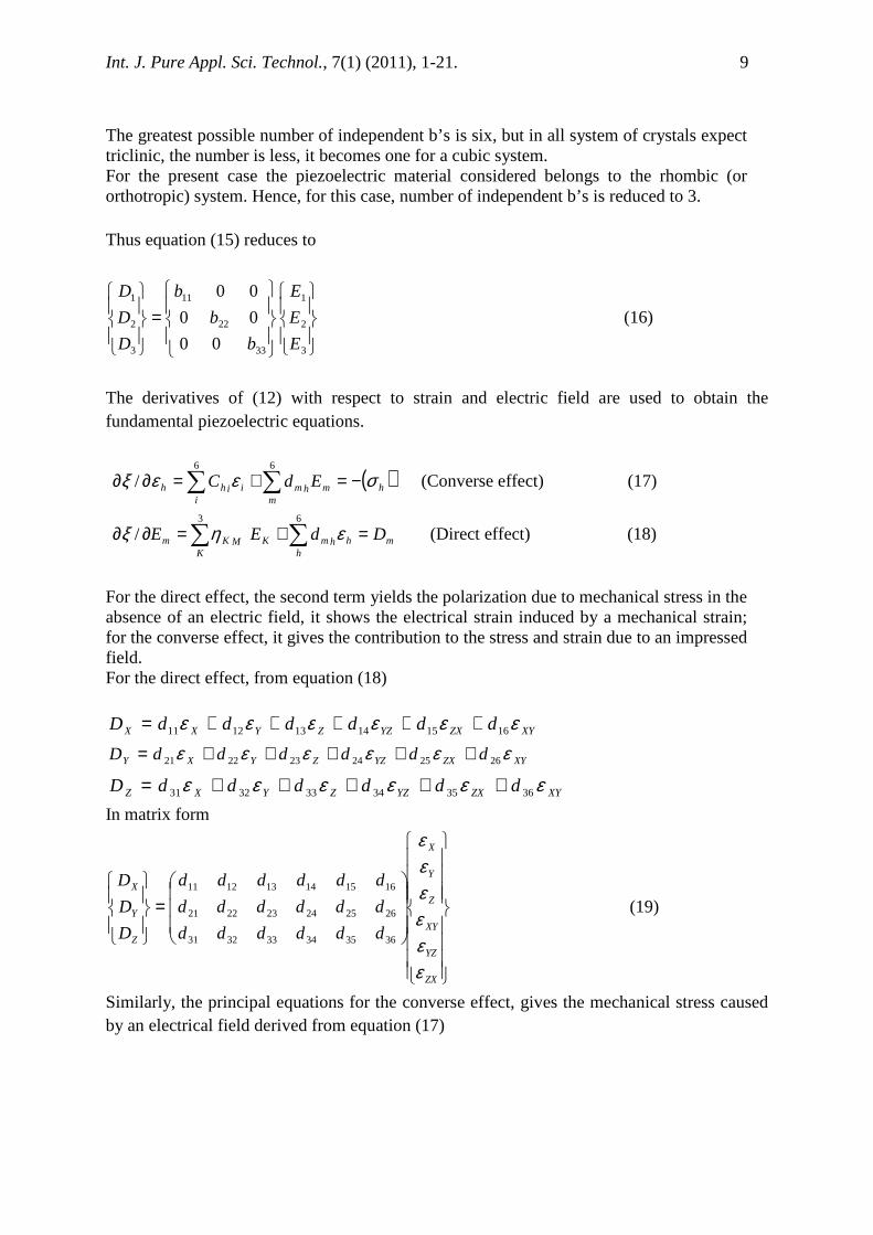
The greatest possible number of independent b’s is six, but in all system of crystals expect triclinic, the number is less, it becomes one for a cubic system. For the present case the piezoelectric material considered belongs to the rhombic (or orthotropic) system. Hence, for this case, number of independent b’s is reduced to 3. Thus equation (15) reduces to
=
3
2
1
33
22
11
3
2
1
00
00
00
E
E
E
b
b
b
D
D
D
(16)
The derivatives of (12) with respect to strain and electric field are used to obtain the fundamental piezoelectric equations.
( )∑ ∑ −=+=∂∂6 6
/i m
hmhmiihh EdC σεεξ (Converse effect) (17)
∑∑ =+=∂∂63
/h
mhhmKK
MKm DdEE εηξ (Direct effect) (18)
For the direct effect, the second term yields the polarization due to mechanical stress in the absence of an electric field, it shows the electrical strain induced by a mechanical strain; for the converse effect, it gives the contribution to the stress and strain due to an impressed field. For the direct effect, from equation (18)
XYZXYZZYXX ddddddD εεεεεε 161514131211 +++++=
XYZXYZZYXY ddddddD εεεεεε 262524232221 +++++=
XYZXYZZYXZ ddddddD εεεεεε 363534333231 +++++=
In matrix form
=
ZX
YZ
XY
Z
Y
X
Z
Y
X
dddddd
dddddd
dddddd
D
D
D
εεεεεε
363534333231
262524232221
161514131211
(19)
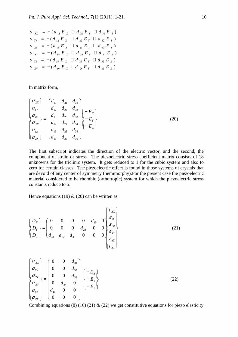
Similarly, the principal equations for the converse effect, gives the mechanical stress caused by an electrical field derived from equation (17)
Int. J. Pure Appl. Sci. Technol., 7(1) (2011), 1-21. 10
)(
)(
)(
)(
)(
)(
362616
352515
342414
332313
322212
312111
ZYXZX
ZYXYZ
ZYXXY
ZYXZZ
ZYXYY
ZYXXX
EdEdEd
EdEdEd
EdEdEd
EdEdEd
EdEdEd
EdEdEd
++−=++−=++−=++−=++−=++−=
σσσσσσ
In matrix form,
=
ZX
YZ
XY
ZZ
YY
XX
σσσσσσ
362616
352515
342414
332313
322212
312111
ddd
ddd
ddd
ddd
ddd
ddd
−−−
Z
Y
X
E
E
E
(20)
The first subscript indicates the direction of the electric vector, and the second, the component of strain or stress. The piezoelectric stress coefficient matrix consists of 18 unknowns for the triclinic system. It gets reduced to 1 for the cubic system and also to zero for certain classes. The piezoelectric effect is found in those systems of crystals that are devoid of any center of symmetry (hemimorphy).For the present case the piezoelectric material considered to be rhombic (orthotropic) system for which the piezoelectric stress constants reduce to 5. Hence equations (19) & (20) can be written as
=
ZX
YZ
XY
ZZ
YY
XX
Z
Y
X
ddd
d
d
D
D
D
εεεεεε
000
00000
00000
333231
24
15
(21)
=
ZX
YZ
XY
ZZ
YY
XX
σσσσσσ
000
00
00
00
00
00
15
24
33
32
31
d
d
d
d
d
−−−
Z
Y
X
E
E
E
(22)
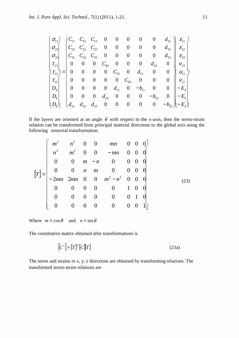
Combining equations (8) (16) (21) & (22) we get constitutive equations for piezo elasticity.
Int. J. Pure Appl. Sci. Technol., 7(1) (2011), 1-21. 11
−−−
−−
−
=
Z
Y
X
Z
Y
X
E
E
E
bddd
bd
bd
C
dC
dC
dCCC
dCCC
dCCC
D
D
D12
13
23
33
22
11
33333231
2224
1115
66
1555
2444
33333231
32232221
31131211
12
13
23
33
22
11
00000
0000000
0000000
00000000
0000000
0000000
00000
00000
00000
νυνεεε
τττσσσ
If the layers are oriented at an angle θ with respect to the x-axis, then the stress-strain relation can be transformed from principal material directions to the global axis using the following tensorial transformation.
[ ]
−−
−−
=
10000000
01000000
00100000
0000022
000000
000000
00000
00000
22
22
22
nmmnmn
mn
nm
mnmn
mnnm
T (23)
Where θcos=m and θsin=n The constitutive matrix obtained after transformations is
[ ] [ ] [ ][ ]TCTC T=* (23a)
The stress and strains in x, y, z directions are obtained by transforming relations. The transformed stress-strain relations are

Int. J. Pure Appl. Sci. Technol., 7(1) (2011), 1-21. 12
−−−
−−
−
=
Z
Y
X
XY
ZX
YZ
ZZ
YY
XX
Z
Y
X
XY
ZX
YZ
ZZ
YY
XX
E
E
E
bddd
bd
bd
C
dC
dC
dCCC
dCCC
dCCC
D
D
D
νννεεε
τττσσσ
*33
*33
*32
*31
*22
*24
*11
*15
*66
*15
*55
*24
*44
33*
33*
32*
31
*32
*23
*22
*21
*31
*13
*12
*11
00000
0000000
0000000
00000000
0000000
0000000
00000
00000
00000
(24)
4.2.6 Variational Formulations
The governing equation of a general weak variational form are derived by making use of the stationanity of total potential energy (functional, as called in variational calculus). The first law of thermodynamics for piezoelectric continuum gives
Iiijij dDEddU += εσ (25)
Where, U is the energy stored/ unit volume in the piezoelectric continuum. The electric enthalpy is defined as
iiO DEUH −= (26)
( )EH O ,ε=
and
jiOij H εσ ∂∂= / and iOji EHD ∂−∂= /
In matrix form
{ } { }εσ ∂∂= /OH and { }EHD O ∂∂−= / (27 &28)
Substituting constitutive equations into equations (27) & (28) and integrating into mechanical and electrical strains respectively yields,
( ) { } [ ]{ } { } [ ] { }EdCH TTTO εεεε −= 2/1
{ } [ ]{ } [ ] [ ]{ }EBEEDEEH TT
O 2/1)( −−=
Combining both the constitutive Equations
( ) { } [ ]{ } { } [ ]{ } [ ] [ ]{ } { } [ ]{ }εεεεε DEEbEEdCEH TTTTO −−−= 2/12/1, (29)
Int. J. Pure Appl. Sci. Technol., 7(1) (2011), 1-21. 13
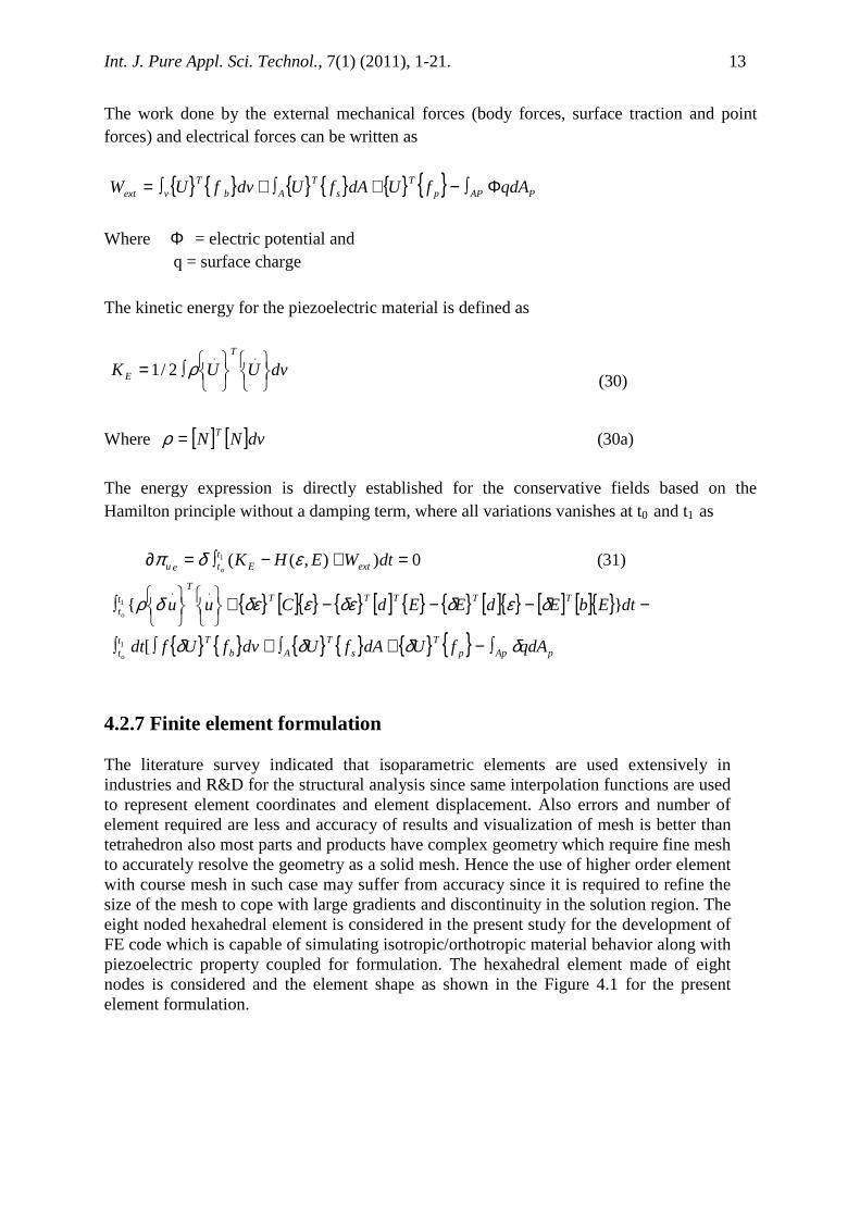
The work done by the external mechanical forces (body forces, surface traction and point forces) and electrical forces can be written as
{ } { } { } { } { } { } PAPpT
sT
AbT
vext qdAfUdAfUdvfUW Φ∫−+∫+∫=
Where Φ = electric potential and q = surface charge The kinetic energy for the piezoelectric material is defined as
dvUUK
T
E
∫=..
2/1 ρ (30)
Where [ ] [ ]dvNN T=ρ (30a)
The energy expression is directly established for the conservative fields based on the Hamilton principle without a damping term, where all variations vanishes at t0 and t1 as
0)),((1 =+−∫=∂ dtWEHK extEtteu o
εδπ (31)
{ } [ ]{ } { } [ ] { } { } [ ]{ } [ ] [ ]{ }
{ } { } { } { } { } { } pAppT
sT
AbTt
t
TTTTTT
tt
qdAfUdAfUdvfUfdt
dtEbEdEEdCuu
o
o
δδδδ
δεδδεεδεδρ
∫−+∫+∫∫
−−−−+
∫
[
}{
1
1
..
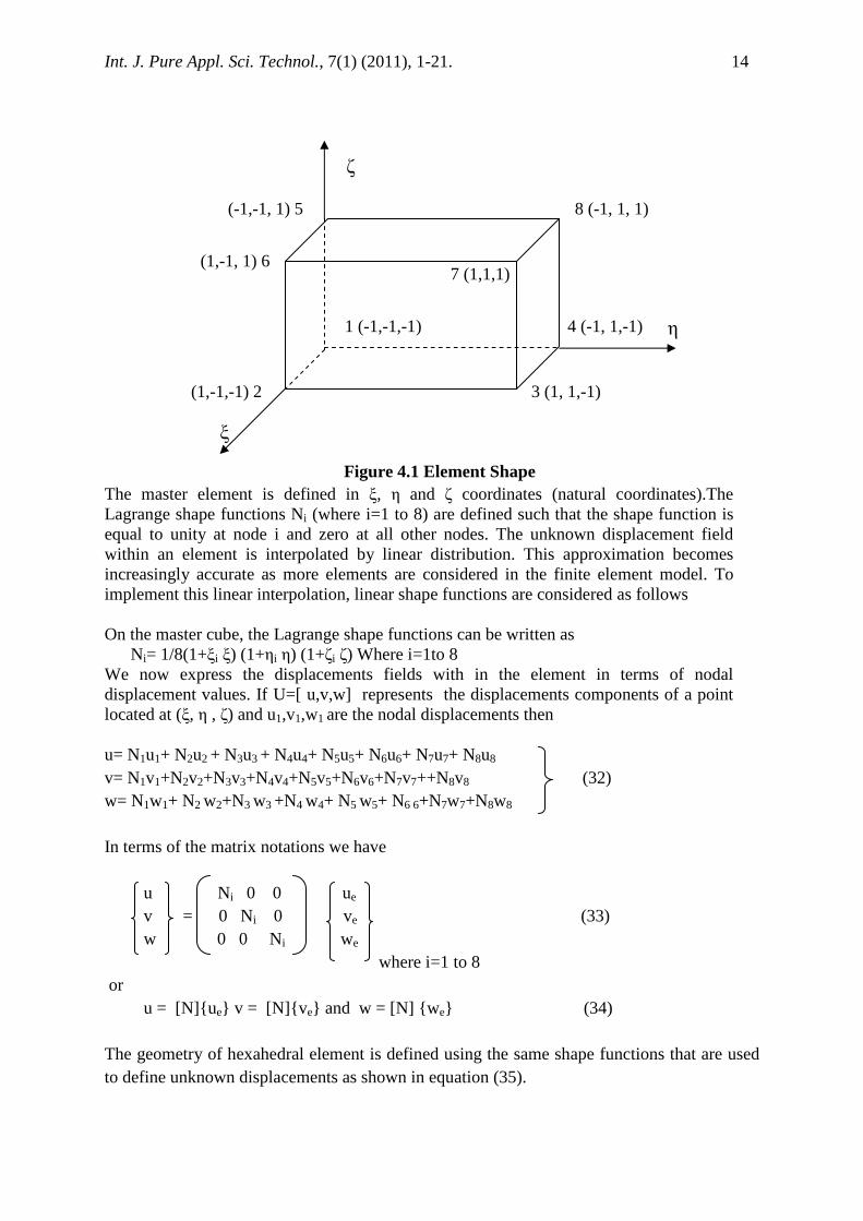
4.2.7 Finite element formulation The literature survey indicated that isoparametric elements are used extensively in industries and R&D for the structural analysis since same interpolation functions are used to represent element coordinates and element displacement. Also errors and number of element required are less and accuracy of results and visualization of mesh is better than tetrahedron also most parts and products have complex geometry which require fine mesh to accurately resolve the geometry as a solid mesh. Hence the use of higher order element with course mesh in such case may suffer from accuracy since it is required to refine the size of the mesh to cope with large gradients and discontinuity in the solution region. The eight noded hexahedral element is considered in the present study for the development of FE code which is capable of simulating isotropic/orthotropic material behavior along with piezoelectric property coupled for formulation. The hexahedral element made of eight nodes is considered and the element shape as shown in the Figure 4.1 for the present element formulation.
Int. J. Pure Appl. Sci. Technol., 7(1) (2011), 1-21. 14
Figure 4.1 Element Shape The master element is defined in ξ, η and ζ coordinates (natural coordinates).The Lagrange shape functions Ni (where i=1 to 8) are defined such that the shape function is equal to unity at node i and zero at all other nodes. The unknown displacement field within an element is interpolated by linear distribution. This approximation becomes increasingly accurate as more elements are considered in the finite element model. To implement this linear interpolation, linear shape functions are considered as follows On the master cube, the Lagrange shape functions can be written as Ni= 1/8(1+ξi ξ) (1+ηi η) (1+ζi ζ) Where i=1to 8 We now express the displacements fields with in the element in terms of nodal displacement values. If U=[ u,v,w] represents the displacements components of a point located at (ξ, η , ζ) and u1,v1,w1 are the nodal displacements then u= N1u1+ N2u2 + N3u3 + N4u4+ N5u5+ N6u6+ N7u7+ N8u8 v= N1v1+N2v2+N3v3+N4v4+N5v5+N6v6+N7v7++N8v8 (32) w= N1w1+ N2 w2+N3 w3 +N4 w4+ N5 w5+ N6 6+N7w7+N8w8 In terms of the matrix notations we have u Ni 0 0 ue
v = 0 Ni 0 ve (33) w 0 0 Ni we
where i=1 to 8 or u = [N]{ue} v = [N]{v e} and w = [N] {we} (34) The geometry of hexahedral element is defined using the same shape functions that are used to define unknown displacements as shown in equation (35).
1 (-1,-1,-1) 4 (-1, 1,-1)
3 (1, 1,-1) (1,-1,-1) 2
(-1,-1, 1) 5
(1,-1, 1) 6 7 (1,1,1)
8 (-1, 1, 1)
η
ξ
ζ
Int. J. Pure Appl. Sci. Technol., 7(1) (2011), 1-21. 15
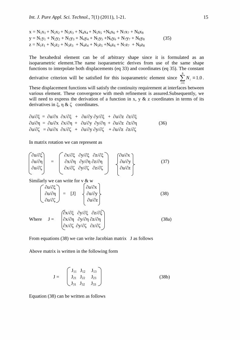
x = N1x1 + N2x2 + N3x3 + N4x4 + N5x5 +N6x6 + N7x7 + N8x8 y = N1y1 + N2y2 + N3y3 + N4y4 + N5y5 +N6y6 + N7y7 + N8y8 (35) z = N1z1 + N2z2 + N3z3 + N4z4 + N5z5 +N6z6 + N7z7 + N8z8
The hexahedral element can be of arbitrary shape since it is formulated as an isoparametric element.The name isoparametric derives from use of the same shape functions to interpolate both displacements (eq 33) and coordinates (eq 35). The constant
derivative criterion will be satisfied for this isoparametric element since 0.18
1
=∑=i
iN .
These displacement functions will satisfy the continuity requirement at interfaces between various element. These convergence with mesh refinement is assured.Subsequently, we will need to express the derivation of a function in x, y & z coordinates in terms of its derivatives in ξ, η & ζ coordinates. ∂u/∂ξ = ∂u/∂x ∂x/∂ξ + ∂u/∂y ∂y/∂ξ + ∂u/∂z ∂z/∂ξ ∂u/∂η = ∂u/∂x ∂x/∂η + ∂u/∂y ∂y/∂η + ∂u/∂z ∂z/∂η (36) ∂u/∂ζ = ∂u/∂x ∂x/∂ζ + ∂u/∂y ∂y/∂ζ + ∂u/∂z ∂z/∂ζ In matrix rotation we can represent as ∂u/∂ξ ∂x/∂ξ ∂y/∂ξ ∂z/∂ξ ∂u/∂x ∂u/∂η = ∂x/∂η ∂y/∂η ∂z/∂η ∂u/∂y (37) ∂u/∂ζ ∂x/∂ζ ∂y/∂ζ ∂z/∂ζ ∂u/∂z Similarly we can write for v & w ∂u/∂ξ ∂u/∂x ∂u/∂η = [J] ∂u/∂y (38) ∂u/∂ζ ∂u/∂z ∂x/∂ξ ∂y/∂ξ ∂z/∂ξ Where J = ∂x/∂η ∂y/∂η ∂z/∂η (38a) ∂x/∂ζ ∂y/∂ζ ∂z/∂ζ From equations (38) we can write Jacobian matrix J as follows Above matrix is written in the following form J11 J12 J13 J = J21 J22 J23 (38b)
J31 J32 J33
Equation (38) can be written as follows
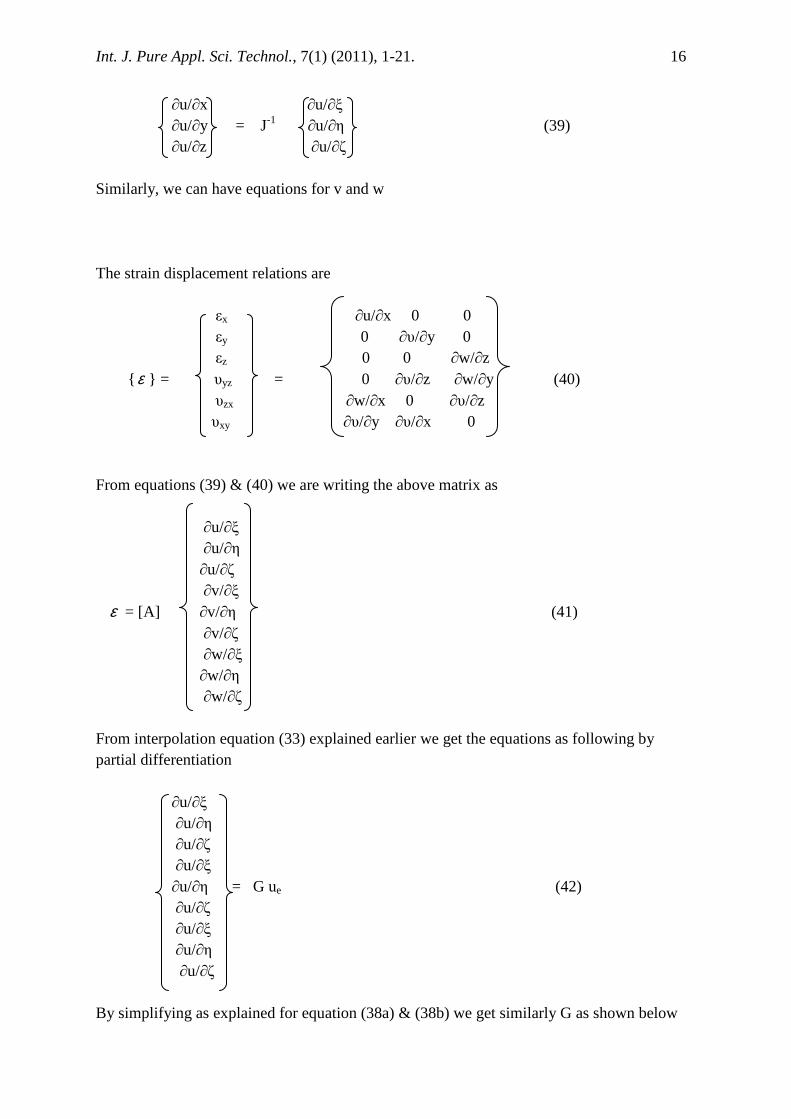
Int. J. Pure Appl. Sci. Technol., 7(1) (2011), 1-21. 16
∂u/∂x ∂u/∂ξ ∂u/∂y = J-1 ∂u/∂η (39) ∂u/∂z ∂u/∂ζ Similarly, we can have equations for v and w The strain displacement relations are εx ∂u/∂x 0 0 εy 0 ∂υ/∂y 0 εz 0 0 ∂w/∂z
{ ε } = υyz = 0 ∂υ/∂z ∂w/∂y (40) υzx ∂w/∂x 0 ∂υ/∂z υxy ∂υ/∂y ∂υ/∂x 0 From equations (39) & (40) we are writing the above matrix as ∂u/∂ξ ∂u/∂η ∂u/∂ζ ∂v/∂ξ ε = [A] ∂v/∂η (41) ∂v/∂ζ ∂w/∂ξ ∂w/∂η ∂w/∂ζ From interpolation equation (33) explained earlier we get the equations as following by partial differentiation ∂u/∂ξ ∂u/∂η ∂u/∂ζ ∂u/∂ξ ∂u/∂η = G ue (42) ∂u/∂ζ ∂u/∂ξ ∂u/∂η ∂u/∂ζ By simplifying as explained for equation (38a) & (38b) we get similarly G as shown below

Int. J. Pure Appl. Sci. Technol., 7(1) (2011), 1-21. 17
G11 G12 G13 G = 1/8 G21 G22 G23 G31 G32 G33 Compare equations (41) & (42) and substitute equation (42) in equation (41). The equation (41) is written as follows { ε } = [A] [G] [ue] (43) Where Rewriting equation (43) { ε } = [B] ue (44) Where B = is the strain displacement matrix for mechanical case u e = nodal displacement ε = Strain matrix
4.2.7.1 Non-piezoelectric case By equation 44 strains is given by { ε } = [B] ue Where B = is the strain displacement matrix for mechanical case ue = nodal displacement and ε = Strain matrix In non piezoelectric case the above formulation are used for coding of the element .Here the element has capability of solving isotropic material such as steel and orthotropic such as composites .The code can solve for both static and dynamic analysis and has three degrees of freedom (Ux, Uy, Uz-mechanical dof) at each node and twenty four degree of freedom per element. The results such as displacement, stresses, reaction and eigenvalues can be obtained from the code.
4.2.7.2 Piezoelectric case The potential function ф0= (x,y,z,t) + Zф1(x,y,z,t) assuming linear variation neglecting curvature effect we get Ф(x,y,z,t) = ф0 (x,y,z,t) Ex ∂ф0/∂x E = Ey = - ∂ф0/∂y Ez ∂ф0/∂z ∂/∂x {E} = - ∂/∂y {ф0} ∂/∂z
B = AG

Int. J. Pure Appl. Sci. Technol., 7(1) (2011), 1-21. 18
{ } [ ]{ }ΦΦ−= ULE (45)
Where { } [ ]{ }euNU ΦΦ=Φ (46)
Substituting (46) in (45) we have
{ } [ ][ ]{ }euNLE ΦΦΦ−=
{ } [ ]{ }euBE ΦΦ−= (47)
Where [[[[ ]]]] [[[[ ]]]]{{{{ }}}}ΦΦΦΦΦΦΦΦΦΦΦΦ ==== NLB Strain displacement matrix for piezoelectric case
W.K.T that relation of nodal displacement and the shape function is as follows
{ } [ ]{ }euNU = (48)
Where N is shape function and ue is nodal displacements. Substituting equations (44), (47) and (30a) into equation (31) into stationary value of the energy equation, which gives the element matrices.
====
++++
ΦΦΦΦΦΦΦΦΦΦΦΦΦΦΦΦ
ΦΦΦΦ
ΦΦΦΦ el
me
e
U
UUU
e
eUU
f
f
u
u
KK
KK
u
u00
0M.
.
(49)
Where
[ ] [ ] [ ][ ]dvBCBK TVuu ∫= Elastic stiffness matrix
[ ] [ ] [ ] [ ]dvBdBK TTVU ΦΦ ∫= Converse piezoelectric stiffness matrix
[ ] [ ] [ ][ ]dvBdBK TVU ΦΦ ∫= Direct piezoelectric stiffness matrix
[ ] [ ] [ ][ ]dvBbBK TV ΦΦΦΦ ∫= Dielectric stiffness matrix
[ ] [ ] [ ]dvNNM TVUU ρρρρ∫= Consistent mass matrix
mf and lef are mechanical, electrical loads respectively.
4.2.8 Condensation of matrices Equation (49) can be written in the following form
[ ]{ } [ ]{ } { }me
ueuu fuKuK =+ ΦΦ (50)
[ ]{ } [ ]{ } { }ele
eu fuKuK =+ ΦΦΦΦ (51)
The electrical degree of freedom can be obtained from equation (51) as follows
{ } [ ] { } [ ] [ ]{ }euele uKKfKu Φ
−ΦΦ
−ΦΦΦ −= 11 (52)
Int. J. Pure Appl. Sci. Technol., 7(1) (2011), 1-21. 19
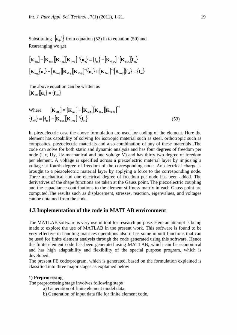
Substituting { }euΦ from equation (52) in to equation (50) and
Rearranging we get
[ ] [ ][ ][ ] { } { } [ ] [ ]{ }leumeuuuu fKKfuKKKK Φ−
ΦΦ−
ΦΦΦΦ −=− 11
The above equation can be written as
[ ]{ } { }effeeff fuK =
Where [ ] [ ] [ ][ ][ ] 1−
ΦΦΦΦ−= KKKKK uuuueff
{ } { } [ ][ ] { }leumeff fKKff 1−ΦΦΦ−= (53)
In piezoelectric case the above formulation are used for coding of the element. Here the element has capability of solving for isotropic material such as steel, orthotropic such as composites, piezoelectric materials and also combination of any of these materials .The code can solve for both static and dynamic analysis and has four degrees of freedom per node (Ux, Uy, Uz-mechanical and one voltage V) and has thirty two degree of freedom per element. A voltage is specified across a piezoelectric material layer by imposing a voltage at fourth degree of freedom of the corresponding node. An electrical charge is brought to a piezoelectric material layer by applying a force to the corresponding node. Three mechanical and one electrical degree of freedom per node has been added. The derivatives of the shape functions are taken at the Gauss point. The piezoelectric coupling and the capacitance contributions to the element stiffness matrix in each Gauss point are computed.The results such as displacement, stresses, reaction, eigenvalues, and voltages can be obtained from the code. 4.3 Implementation of the code in MATLAB environment The MATLAB software is very useful tool for research purpose. Here an attempt is being made to explore the use of MATLAB in the present work. This software is found to be very effective in handling matrices operations also it has some inbuilt functions that can be used for finite element analysis through the code generated using this software. Hence the finite element code has been generated using MATLAB, which can be economical and has high adaptability and flexibility of the special purpose program, which is developed. The present FE code/program, which is generated, based on the formulation explained is classified into three major stages as explained below 1) Preprocessing The preprocessing stage involves following steps
a) Generation of finite element model data. b) Generation of input data file for finite element code.
[ ]{ } [ ][ ][ ] { } [ ] [ ]{ } { }melueuueuu ffKKuKKKuK =+− Φ−
ΦΦ−
ΦΦΦΦ11

Int. J. Pure Appl. Sci. Technol., 7(1) (2011), 1-21. 20
2) Processing The processing stage involves following steps
a) Evaluating elemental matrices namely stiffness matrix , mass matrix, and load vector.
b) Assembly of the elemental matrices to form global matrices. c) Application of boundary condition. d) Solution of the above modified equations.
3) Post processing The post processing stage involves the following steps a) Computation of stresses, strains, reactions and voltages, done through the built-in matrix manipulation.
b) Printing of displacement, stress, voltages etc. Only FE model is generated outside the code using Ansys and the input data file is generated using MATLAB editor manually by using the mesh data such as nodal coordinates and element connectivity from Ansys. The other details such as boundary conditions are given to the input data file manually using MATLAB editor. The generation of various finite element related matrices and vectors are carried out by using the developed code including the computation of results for structural and electromechanical analysis of smart structures. The input data file is generated consisting of following set of data
a) Model definition : Geometry data (i.e. node coordinates) b) Element data : Type of element, connectivity, material. c) Degree of freedom data: Forces, boundary condition and voltage.
The code has main program and functions, which are explained as follows The main program and functions for the finite element code is generated using MATLAB. The function or subroutine program will be called by statements in main program to carry out desired computation. The program reads data from input file and process using various functions that is developed. Some of the important functions are used to do the following
a) To read input data file. b) To compute element stiffness matrix for isotropic, orthotropic and piezoelectric
case. c) To assemble element stiffness matrix to global stiffness matrix. d) To compute element mass matrix for isotropic, orthotropic and piezoelectric case. e) To assemble element mass matrix to global mass matrix. f) To apply constraints to global stiffness matrix. g) To apply constraints to global mass matrix. h) To compute results such as displacements, stresses, voltage, natural frequencies
for both elastic and piezoelectric case. 5. Conclusions The finite element analysis is a useful technique for carrying out the structural and electromechanical analysis. It appears that a very little published information is available
Int. J. Pure Appl. Sci. Technol., 7(1) (2011), 1-21. 21
in the area of development of finite element for structural and electromechanical of a three dimensional piezoelectric composite structures using finite element technique. Hence in the present work development( formulation and programming) of a eight noded hexahedral element finite element for structural and electromechanical analysis has been carried out using MATLAB software. The finite element code, which is based on this formulation generated, can analyze isotropic materials such as steel, aluminum and orthotropic materials such as composites and piezoelectric structures. References [1] Chien-chang Lin, Vibration control of beam-plates with bonded piezoelectric sensors and
actuators, J of Computers and Structures, 73 (1999), 239-248. [2] Chang Ho Hong and Inderjith chopra, Modelling and validation of induced strain
actuation of composite coupled plate, AIAA J, 37 (1999), 372-377. [3] Ho-Jun Hee and D. A. Sanavanos, Coupled layer wise analysis of thermo piezoelectric
composite beams, AIAA J, 34 (1997). [4] C. K. Gim, Plate finite element modeling of laminated plates, Computers and structures,
52 (1) (1994), 157-168. [5] T. S. Tzou and C. I. Tsen, Distributed piezoelectric sensor/actuators design for dynamic
measurement/control of distributed parameter systems - a piezoceramic finite element approach, J of Sound Vibrations,1990
[6] A. Trindade, A. Benjeddo and Ohayon, Finite element modeling of hybrid active-passive vibration damping of multiplayer piezoelectric sandwich beams- part I : formulation, part II : system analysis, International J for Numerical Methods in Engineering,51 (2001), 835-864.
[7] Aditi Chattopadhyay, Haozhong Gu and Rajan Beri, Modelling segmented active constrained layer damping using hybrid displacement field, AIAA J, 39 (2001), 480-486.
[8] U. O. Akpan, T. S. Koko, I. R. Orisamolu and B. K. Gallart, Fuzzy finite-element analysis of smart structures, J of Smart Materials and Structures, 10 (2001), 273 – 284.
[9] J. Lopez-Bonilla, Lanczos derivative via a quadrature method, Int. J. Pure Appl. Sci. Technol., 1(2) (2010), 100-103.
[10] Sung kyu and Charles Keillers, Finite element analysis of composite structures containing distributed piezoceramic sensors and actuators, AIAA J, 30 (3) (1992).