Destabilizing a stable crisis: employment persistence and governmentintervention in macroeconomics

B. Costa Limaa, M. R. Grassellia, X-S. Wangb, J. Wub

aDepartment of Mathematics and Statistics, McMaster University, Hamilton ON L8S 4K1, CanadabDepartment of Mathematics and Statistics, York University, Toronto ON M3J 1P3, Canada

Abstract

The basic Keen model is a three-dimensional dynamical system describing the time evo-lution of the wage share, employment rate, and private debt in a closed economy. In theabsence of government intervention this system admits, among others, two locally stableequilibria: one with a finite level of debt and nonzero wages and employment rate, andanother characterized by infinite debt and vanishing wages and employment. We show howthe addition of a government sector, modelled through appropriately selected functions de-scribing spending and taxation, prevents the equilibrium with infinite debt. Specifically,we show that, by countering the fall in private profits with sufficiently high governmentspending at low employment, the extended system can be made uniformly weakly persis-tent with respect to the employment rate. In other words, the economy is guaranteed notto stay in a permanently depressed state with arbitrarily low employment rates.

Keywords: Government intervention, persistence, Keen model, stock-flow consistency.JEL: C65, E24, E62, G01

1. Introduction

Among the many unintended consequences of the financial crisis of 2007-08, a pleasantlysurprising one was the emergence of a Minsky revival. From Wall Street analysts to majornewspapers to repentant mainstream economists, the ideas of Hyman Minsky attractedwidespread interest because of the prescient and precise way in which they helped explainunfolding events. The term “Minsky crisis” was quickly coined to describe the processesleading up to the observed financial fragility and its consequences for the real economy.As highlighted by Wray (2011) in the New Palgrave Dictionary entry explaining the term,at the core of Minsky’s analysis is the role of institutional ceilings and floors in stabilizing

∗Corresponding author. Tel.: +1 905 525 9140 ext 23406; fax: +1 905 522-0935.Email address: grasselli@math.mcmaster.ca (M. R. Grasselli)

Preprint submitted to Structural Change and Economic Dynamics August 2, 2013

the inherently explosive dynamics of capitalist economies. The purpose of this paper isto investigate these stabilizing effects using the modern tools of persistence theory fordynamical systems.

Mathematical formalizations of Minsky’s ideas are not exactly abundant, but are nonethe-less identifiable as a growing strand in the economics literature. A useful survey up to 2005is presented in Dos Santos (2005) and more recent contributions include Ryoo (2010) andChiarella and Guilmi (2011). The vast majority of papers in this area, however, focuson the dynamic relationships that can lead to instability and explosive behaviour for theunderlying variables, with the role of government somewhat restricted to playing secondfiddle, say through regulation or by issuing bonds that can enter the portfolio decisions ofmore active players, such as firms and households. For example, as explained in Dos Santos(2005), because government policy is not specified in sufficiently complete way in the influ-ential early paper by Taylor and O’Connell (1985), the consequences of several “hidden”hypotheses that are necessary for stock-flow consistency issues are not fully analyzed. Bycontrast, we model government intervention explicitly and thoroughly analyze its relation-ships with the other dynamic variables in the economy.

After setting up a simplified yet sufficiently general closed system of accounts for house-holds, firms, banks and the government sector in Section 2, we start by reviewing the specialcase of a model proposed in Keen (1995). In the absence of a government sector, the Keenmodel consists of the three-dimensional system (14) describing the dynamics of wages,employment rate and private debt. Its key insight is that, in boom times when profitsare high, capitalists can choose to invest more than their profits by borrowing from thebanking sector. If profits are low, on the other hand, capitalists might also want to investless than their profits to pay down debt, thereby engaging in the familiar debt-deflationdynamics described in Fisher (1933). As shown in Grasselli and Costa Lima (2012), thisbehaviour by capitalists leads to the possibility of two very distinct equilibria recalled inSection 3.1: a “good equilibrium” characterized by finite private debt and nonzero wageshare and employment rate, and a “bad equilibrium” characterized by infinite private debtand vanishing wage share and employment rate. Moreover, for typical parameter values,both equilibria are locally stable.

As emphasized throughout Minsky (1982), the debt-deflation mechanism can be haltedby government intervention, since it follows from Kalecki’s profit equation that govern-ment spending increases firm profits. We formalize this insight by introducing governmentexpenditures, subsidies, and taxation into the Keen model in Section 2.2. Governmentintervention had already been proposed in Keen (1995), albeit in a different functionalform. The key variable for firm behaviour is the profit share of output π given in (30),which depends on government policy only through subsidies and taxations, but not throughexpenditures, since the latter is part of total output. After isolating the core variables inthe model from those whose evolution can be obtained separately, we are left with thefive-dimensional system described by (32) for wage share, employment rate, stimulativesubsidies and taxation, and profit share.

2

We perform local analysis for this system in Section 3. As before, we find a finite-value “good equilibrium” associated with non-zero wage share and employment rate andfinite private debt. All other finite-value equilibria turn out to be related to vanishingwage shares, but none is locally stable for typical parameter values. We next move tothe characterization of “bad equilibria”, that is, those associated with collapsing profitshares even in the presence of government intervention. We find in Proposition 1 thatprovided the size of government subsidies in the vicinity of zero employment rates is largeenough, all of these bad equilibria are either unstable or unachievable, even when the localstability condition for the corresponding bad equilibrium in the model without governmentis satisfied. In other words, government intervention successfully destabilizes an otherwisestable equilibrium point associated with an economic crises.

Our main results are contained in Section 4. Persistence theory (see Smith and Thieme,2011) studies the long term behaviour of dynamical systems, in particular the possibilitythat one or more variables remain bounded away from zero. Typical questions are, forexample, which species in a model of interacting species will survive over the long term,or whether in an endemic model an infection cannot persist in a population due to thedepletion of the susceptible population. In our context, we are interested in establishingconditions in economic models that prevent one or more key economic variables, such asthe employment rate, from vanishing. After preliminary technical results for profit levelsin Propositions 2 and 3, we prove in Proposition 4 that under a variety of alternative mildconditions on government subsidies, the model describing the economy is uniformly weaklypersistent with respect to the employment rate λ. The relevant precise definitions of per-sistence are reviewed in Appendix C, but the meaning of this result is easy enough toconvey: we can guarantee that the employment rate does not remain indefinitely trappedat arbitrarily small values. This is in sharp contrast with what happens in the model with-out government intervention, where the employment rate is guaranteed to converge to zeroand remain there forever if the initial conditions are in the basin of attraction of the badequilibrium corresponding to infinite debt levels. Furthermore, as any persistence result,Proposition 4 is a global one: no matter how disastrous the initial conditions are, a suffi-ciently responsive government can bring the economy back from a state of crises associatedwith zero employment rates. We end the paper with numerical examples illustrating theseresults in Section 5.

2. Derivation of the model

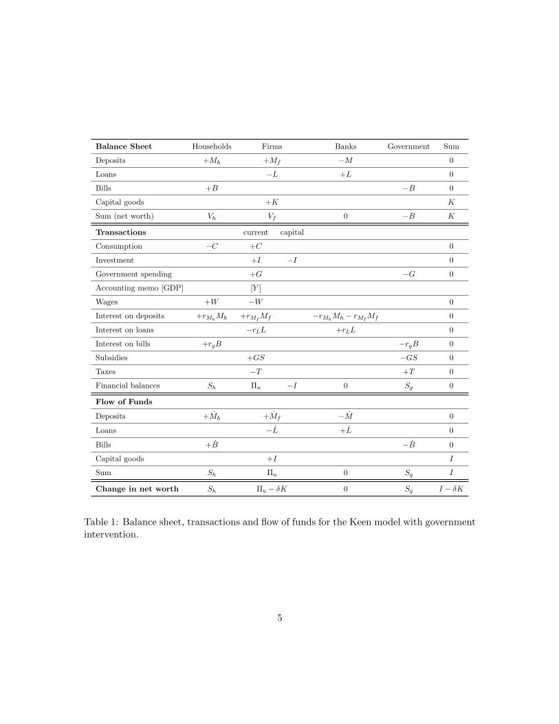
We consider the closed system of accounts shown in Table 1, where each entry rep-resents a time-dependent quantity and a dot corresponds to differentiation with respectto time. As usual, balance sheet items are stocks measured in units of account, whereasboth transactions and flow of funds items as flows measured in units of account per unitof time. For example, going down the first column, Mh ≡ Mh(t), rMh

Mh ≡ rMh(t)Mh(t),

3

and Mh ≡ Mh(t) denote, respectively, the amount, the flow of interest payments, and therate of change associate with deposits held by households at time t.

We see from Table 1 that the entire economy is subdivided in the Households, Firms,Banks, and Government sectors. Their balance sheet structure is fairly simple: the assetsof households are bank deposits Mh and government debt B; the assets of firms are bankdeposits Mf and capital goods K and they have liabilities in the form of bank loans L;banks have total deposits M = Mh + Mf as their only liabilities and loans L as theironly assets; government debt B is the only liability of the government sector. The emptycells in Table 1 represent the following simplifying assumptions: households do not makebank loans; the government sector does not keep bank deposits or make bank loans; firmsand banks do not hold government debt. The absence of equities as a balance sheet itemcorresponds to the following further simplifications in the ownership structure of banks andfirms: neither sector issues or hold equities; the net worth of firms is the difference betweencapital and net debt to the banking sector; the net worth of banks is kept identically zeroat all times. In particular, we have that

D := L−Mf = Mh. (1)

Most of the transactions items in Table 1 are self-explanatory, except for our treatmentof taxes and subsidies, which we assume to be restricted to the firms sector. This is becausethe main goal of this paper is to show how the government sector can effectively prevent acrisis caused by the collapse of firm profits. Because transfer payments to households andtaxes from households do not play a significant role in this dynamics, we chose to leavethem out of the transaction flows, since including them would not affect the results.

The only other nontrivial assumption about transactions refer to the rate of intereston loans and deposits. Consistently with our hypothesis of zero net worth for banks, theinterest rate rMh

paid to household deposits need to be related to the rates rMfand rL for

firm deposits and loans as follows:

rMhMh = rMf

Mf − rLL. (2)

Accordingly, since Mh = D = L −Mf , the net flow of interest payments from firms tobanks equal rMh

D.The flow of funds presented in Table 1 reflect the stock-flow consistency condition:

financial balances for each sector are used to change their holdings of balance-sheet items.For example, central to the model is the fact that firms finance investment using both theirfinancial balance and net borrowing from the banking sector according to the accountingidentity

I −Πu = L− Mf = D. (3)

All the quantities in Table 1 are given in real rather than nominal terms, that is to say,already divided by an agreed price deflator.

4

Balance Sheet Households Firms Banks Government Sum

Deposits +Mh +Mf −M 0

Loans −L +L 0

Bills +B −B 0

Capital goods +K K

Sum (net worth) Vh Vf 0 −B K

Transactions current capital

Consumption −C +C 0

Investment +I −I 0

Government spending +G −G 0

Accounting memo [GDP] [Y ]

Wages +W −W 0

Interest on deposits +rMhMh +rMf

Mf −rMhMh − rMf

Mf 0

Interest on loans −rLL +rLL 0

Interest on bills +rgB −rgB 0

Subsidies +GS −GS 0

Taxes −T +T 0

Financial balances Sh Πu −I 0 Sg 0

Flow of Funds

Deposits +Mh +Mf −M 0

Loans −L +L 0

Bills +B −B 0

Capital goods +I I

Sum Sh Πu 0 Sg I

Change in net worth Sh Πu − δK 0 Sg I − δK

Table 1: Balance sheet, transactions and flow of funds for the Keen model with governmentintervention.

5

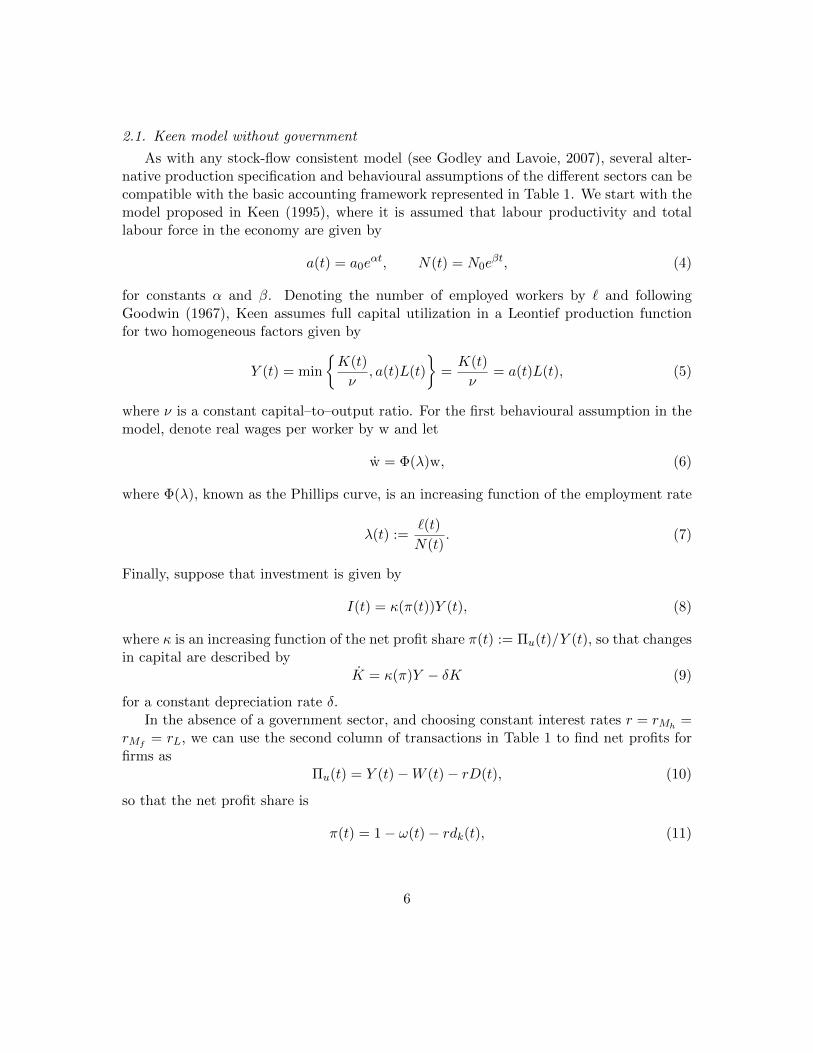
2.1. Keen model without government

As with any stock-flow consistent model (see Godley and Lavoie, 2007), several alter-native production specification and behavioural assumptions of the different sectors can becompatible with the basic accounting framework represented in Table 1. We start with themodel proposed in Keen (1995), where it is assumed that labour productivity and totallabour force in the economy are given by

a(t) = a0eαt, N(t) = N0e

βt, (4)

for constants α and β. Denoting the number of employed workers by ` and followingGoodwin (1967), Keen assumes full capital utilization in a Leontief production functionfor two homogeneous factors given by

Y (t) = min

{K(t)

ν, a(t)L(t)

}=K(t)

ν= a(t)L(t), (5)

where ν is a constant capital–to–output ratio. For the first behavioural assumption in themodel, denote real wages per worker by w and let

w = Φ(λ)w, (6)

where Φ(λ), known as the Phillips curve, is an increasing function of the employment rate

λ(t) :=`(t)

N(t). (7)

Finally, suppose that investment is given by

I(t) = κ(π(t))Y (t), (8)

where κ is an increasing function of the net profit share π(t) := Πu(t)/Y (t), so that changesin capital are described by

K = κ(π)Y − δK (9)

for a constant depreciation rate δ.In the absence of a government sector, and choosing constant interest rates r = rMh

=rMf

= rL, we can use the second column of transactions in Table 1 to find net profits forfirms as

Πu(t) = Y (t)−W (t)− rD(t), (10)

so that the net profit share is

π(t) = 1− ω(t)− rdk(t), (11)

6

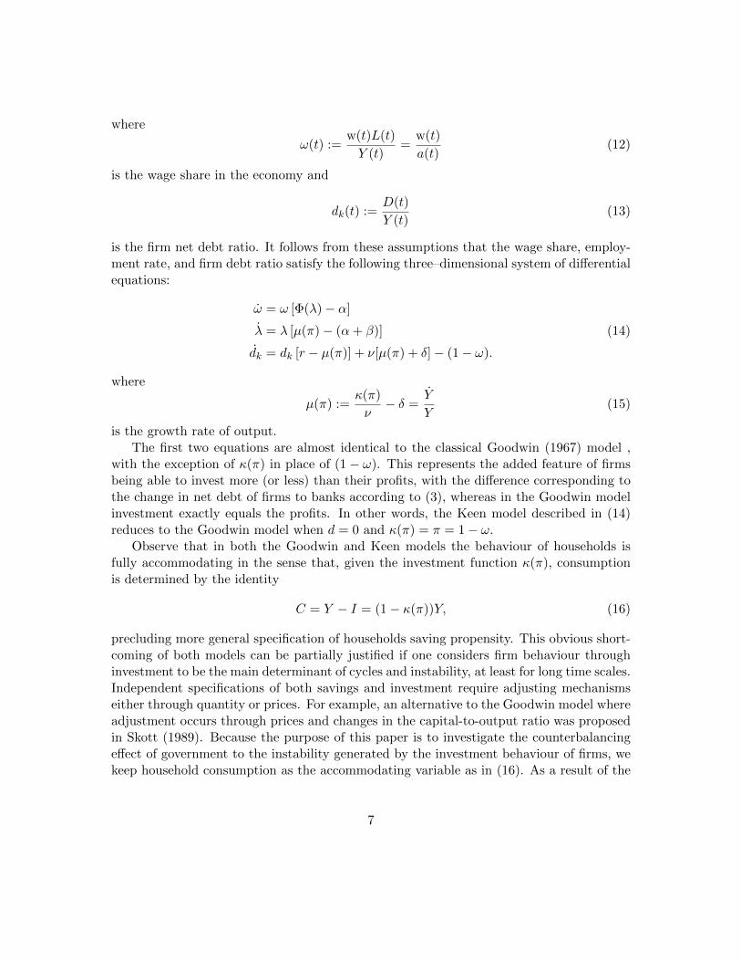
where

ω(t) :=w(t)L(t)

Y (t)=

w(t)

a(t)(12)

is the wage share in the economy and

dk(t) :=D(t)

Y (t)(13)

is the firm net debt ratio. It follows from these assumptions that the wage share, employ-ment rate, and firm debt ratio satisfy the following three–dimensional system of differentialequations:

ω = ω [Φ(λ)− α]

λ = λ [µ(π)− (α+ β)]

dk = dk [r − µ(π)] + ν[µ(π) + δ]− (1− ω).

(14)

where

µ(π) :=κ(π)

ν− δ =

Y

Y(15)

is the growth rate of output.The first two equations are almost identical to the classical Goodwin (1967) model ,

with the exception of κ(π) in place of (1− ω). This represents the added feature of firmsbeing able to invest more (or less) than their profits, with the difference corresponding tothe change in net debt of firms to banks according to (3), whereas in the Goodwin modelinvestment exactly equals the profits. In other words, the Keen model described in (14)reduces to the Goodwin model when d = 0 and κ(π) = π = 1− ω.

Observe that in both the Goodwin and Keen models the behaviour of households isfully accommodating in the sense that, given the investment function κ(π), consumptionis determined by the identity

C = Y − I = (1− κ(π))Y, (16)

precluding more general specification of households saving propensity. This obvious short-coming of both models can be partially justified if one considers firm behaviour throughinvestment to be the main determinant of cycles and instability, at least for long time scales.Independent specifications of both savings and investment require adjusting mechanismseither through quantity or prices. For example, an alternative to the Goodwin model whereadjustment occurs through prices and changes in the capital-to-output ratio was proposedin Skott (1989). Because the purpose of this paper is to investigate the counterbalancingeffect of government to the instability generated by the investment behaviour of firms, wekeep household consumption as the accommodating variable as in (16). As a result of the

7

closed system of accounts presented in Table 1 we have that, in the absence of government,household savings satisfy

Mh = Sh = W + rMh − C = W + rD − Y + I = I −Πu = D, (17)

so that investment equals total savings, and the change in net debt of firms to the banksector equals the change in household deposits.

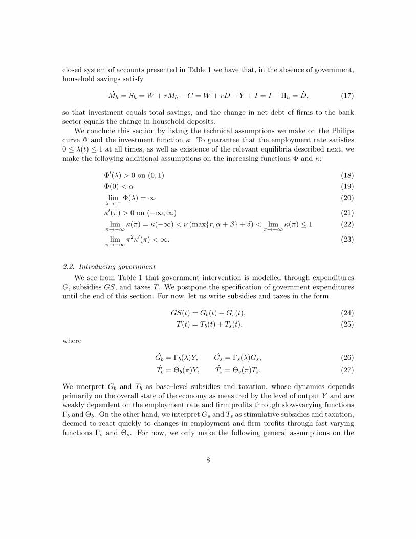
We conclude this section by listing the technical assumptions we make on the Philipscurve Φ and the investment function κ. To guarantee that the employment rate satisfies0 ≤ λ(t) ≤ 1 at all times, as well as existence of the relevant equilibria described next, wemake the following additional assumptions on the increasing functions Φ and κ:

Φ′(λ) > 0 on (0, 1) (18)

Φ(0) < α (19)

limλ→1−

Φ(λ) =∞ (20)

κ′(π) > 0 on (−∞,∞) (21)

limπ→−∞

κ(π) = κ(−∞) < ν (max{r, α+ β}+ δ) < limπ→+∞

κ(π) ≤ 1 (22)

limπ→−∞

π2κ′(π) <∞. (23)

2.2. Introducing government

We see from Table 1 that government intervention is modelled through expendituresG, subsidies GS, and taxes T . We postpone the specification of government expendituresuntil the end of this section. For now, let us write subsidies and taxes in the form

GS(t) = Gb(t) +Gs(t), (24)

T (t) = Tb(t) + Ts(t), (25)

where

Gb = Γb(λ)Y, Gs = Γs(λ)Gs, (26)

Tb = Θb(π)Y, Ts = Θs(π)Ts. (27)

We interpret Gb and Tb as base–level subsidies and taxation, whose dynamics dependsprimarily on the overall state of the economy as measured by the level of output Y and areweakly dependent on the employment rate and firm profits through slow-varying functionsΓb and Θb. On the other hand, we interpret Gs and Ts as stimulative subsidies and taxation,deemed to react quickly to changes in employment and firm profits through fast-varyingfunctions Γs and Θs. For now, we only make the following general assumptions on the

8

subsidies and taxation structural functions:

Γ′b(λ) < 0 and Γ′s(λ) < 0 on (0, 1) (28)

Θ′b(π) > 0 and Θ′s(π) > 0 on (−∞,∞). (29)

Defining gb = Gb/Y , gs = Gs/Y , τb = Tb/Y , τs = Ts/Y , it follows that the profit shareof firms is now

π(t) = 1− ω(t)− rdk(t) + gb(t) + gs(t)− τb(t)− τs(t). (30)

A bit of algebra leads to the following seven–dimensional system:

ω = ω [Φ(λ)− α]

λ = λ [µ(π)− α− β]

dk = νµ(π) + νδ − π − dkµ(π)

gb = Γb(λ)− gbµ(π)

τb = Θb(π)− τbµ(π)

gs = gs [Γs(λ)− µ(π)]

τs = τs [Θs(π)− µ(π)] .

(31)

Observe now that we can write

π = −ω − rdk + gb + gs − τb − τs= −ω(Φ(λ)− α)− r(νµ(π) + νδ − π) + Γb(λ) + gsΓs(λ)−Θb(π)− τsΘs(π) + (rdk − g + τ)µ(π)

= −ω(Φ(λ)− α)− r(νµ(π) + νδ − π) + (1− ω − π)µ(π) + Γb(λ) + gsΓs(λ)−Θb(π)− τsΘs(π),

so that the previous system reduces to the five-dimensional system

ω =ω [Φ(λ)− α]

λ =λ [µ(π)− α− β]

gs =gs [Γs(λ)− µ(π)]

τs =τs [Θs(π)− µ(π)]

π =− ω(Φ(λ)− α)− r(νµ(π) + νδ − π) + (1− ω − π)µ(π)

+ Γb(λ) + gsΓs(λ)−Θb(π)− τsΘs(π).

(32)

In other words, since the variables (dk, gb, τb) do not affect the dynamics of the variables(ω, λ, gs, τs, π), the reduced system (32) can be solved separately. Moreover, the trajectories(π(t), λ(t)) arising as solutions of (32) can be treated as time-dependent coefficients for the

9

remaining uncoupled differential equations

dk = νµ(π) + νδ − π − dkµ(π)

gb = Γb(λ)− gbµ(π)

τb = Θb(π)− τbµ(π)

(33)

In particular, if the system (32) is at an equilibrium state (ω, λ, gs, τs, π), then the remainingvariables must converge exponentially fast, with rate µ(π), to their equilibrium values

dk =νµ(π) + νδ − π

µ(π), gb =

Γb(λ)

µ(π), τ b =

Θb(π)

µ(π). (34)

We shall base our analytic results on the reduced system (32), since this will be enoughto characterize the equilibria in which the economy either prospers or collapses. Observethat when working with the reduced system (32), we cannot recover dk, gb and τb separately,but rather the combination

rdk − gb + τb = 1− ω − π + gs − τs . (35)

For numerical simulations, however, we compute the trajectories for the full system (31),so that the evolution of each individual variable can be followed separately.

We now return to the specification of government expenditures G. Observe that, sinceG does not affect the profit share in (30), its dynamics can be freely chosen without alteringthe solution of either the reduced system (32) or the full system (31). In fact, the onlyother variable affected by G is government debt, which according to Table 1, satisfies

B = rgB +G+GS − T. (36)

For example, if we define dg = B/Y and ge = G/Y and postulate the dynamics forexpenditures in the form

G = Γ(t, ω, λ, π, gs, τs, G, Y ), (37)

we obtain

ge =Γ(ω, λ, π, gs, τs, G, Y )

Y− geµ(π) (38)

dg = ge + gb + gs − τb − τs − dg (µ(π)− r) . (39)

In other words, as long as the dynamics for government expenditures does not dependexplicitly on the level of government debt, equation (38) can be solved separately first andthen used to solve equation (39). Equivalently, we can model the government expenditureratio directly as a function ge = ge(t, ω, λ, π, gs, τs). In either case, if the governmentexpenditure ratio is at an equilibrium value ge compatible with equilibrium values for the

10

remaining variables, then the government debt ratio converges exponentially fast, with rateµ(π)− r, to the equilibrium value

dg =

ge + gb + gs − τ b − τ s

µ(π)− rif r < µ(π)

+∞ if r > µ(π), or r = µ(π) and ge + gb + gs > τ b + τ s

0 if r = µ(π) and ge + gb + gs < τ b + τ s

(40)As before, the behaviour of households is fully accommodating in the sense that, giventhe investment function κ(π) and the government expenditure ratio ge, consumption byhouseholds is determined by the identity

C = Y − I −G = (1− κ(π)− ge)Y. (41)

3. Equilibrium Analysis

3.1. Keen model without government

As shown in Grasselli and Costa Lima (2012), there are three relevant equilibria for(14). The first one is given by ω0 = λ0 = 0 and d0 solving the equation

d

[r + δ − κ(1− rd)

ν

]= 1− κ(1− rd). (42)

This is locally unstable for typical parameter values and corresponds to the economicallyuninteresting case of a crashed economy with finite debt.

The second one, hereafter called the “good equilibrium” is given by

ω1 = 1− π1 −r(κ(π1)− π1)

α+ β

λ1 = Φ−1(α)

d1 =ν(α+ β + δ)− π1

α+ β

(43)

withπ1 = κ−1(ν(α+ β + δ)). (44)

The necessary and sufficient condition for its local stability is

r

[κ′(π1)

ν(π1 − κ(π1) + ν(α+ β))− (α+ β)

]> 0, (45)

which is satisfied by a wide range of parameter values.

11

The third equilibrium, henceforth referred to as the “bad equilibrium”, is defined by

ω2 = 0

λ2 = 0

d2 → +∞(46)

and is locally stable if and only if

µ(−∞) =κ(−∞)

ν− δ < r. (47)

Observe that (47) is easily satisfied, since κ(−∞) is the rate of investment when capitalistsface large negative profits and can be safely assumed to be very small. In what follows, weargue that government intervention in the form of spending and taxation is an effective wayto prevent the system from reaching this undesirable equilibrium of vanishing employment,vanishing wages, and exploding private debt.

3.2. Finite-valued equilibria with government

The hyperplanes gs = 0 and τs = 0 are invariant manifolds for (32), indicating thatif the initial value for either gs or τs is positive (or negative), the corresponding solutionis entirely contained in that quadrant. Typically, gs > 0 and τs ≤ 0, as the governmentattempts to stimulate the economy with a mixture of subsidies and tax cuts, although onecould have gs ≤ 0 and/or τs > 0 in the case of austerity measures intended to reduce thegovernment deficit (as a naive attempt to decrease government debt) when the economyperforms badly.

To find the first equilibrium, let

λ1 = Φ−1(α)

π1 = µ−1(α+ β)(48)

so that ω = λ = 0. Discarding the structural coincidences Γs(λ1) = α+β or Θs(π1) = α+β,the only way to obtain gs = τs = 0 is to set gs1 = τ s1 = 0. This leads us to

ω1 = 1− π1 −r(ν(α+ β + δ)− π1)

α+ β+

Γb(λ1)−Θb(π1)

α+ β(49)

as the only way to obtain π = 0. This defines what we call the “good equilibrium” for(32), that is, an equilibrium characterized by finite values for all variables and non-zerowage share.

As show in Appendix A, all remaining finite-valued equilibria (32) have the wage shareequal to zero. To summarize, discarding equilibria whose existence depend on structurallyunstable coincidences in the choice of parameter values, the finite-valued equilibria for

12

system (32) are given by

(ω, λ, gs, τs , π) =

(ω1, λ1, 0, 0, π1)

(0, λ2, gs2, 0, π1)

(0, λ3, 0, 0, π1)

(0, 0, 0, 0, π4)

(0, 0, 0, τ s5, π5)

(0, 0, gs6, 0, π6),

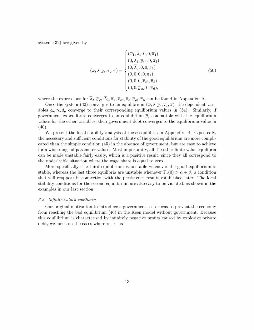
(50)

where the expressions for λ2, gs2, λ3, π4, τ s5, π5, gs6, π6 can be found in Appendix A.Once the system (32) converges to an equilibrium (ω, λ, gs, τ s , π), the dependent vari-

ables gb, τb, dg converge to their corresponding equilibrium values in (34). Similarly, ifgovernment expenditure converges to an equilibrium ge compatible with the equilibriumvalues for the other variables, then government debt converges to the equilibrium value in(40).

We present the local stability analysis of these equilibria in Appendix B. Expectedly,the necessary and sufficient conditions for stability of the good equilibrium are more compli-cated than the simple condition (45) in the absence of government, but are easy to achievefor a wide range of parameter values. Most importantly, all the other finite-value equilibriacan be made unstable fairly easily, which is a positive result, since they all correspond tothe undesirable situation where the wage share is equal to zero.

More specifically, the third equilibrium is unstable whenever the good equilibrium isstable, whereas the last three equilibria are unstable whenever Γs(0) > α+ β, a conditionthat will reappear in connection with the persistence results established later. The localstability conditions for the second equilibrium are also easy to be violated, as shown in theexamples in our last section.

3.3. Infinite-valued equilibria

Our original motivation to introduce a government sector was to prevent the economyfrom reaching the bad equilibrium (46) in the Keen model without government. Becausethis equilibrium is characterized by infinitely negative profits caused by explosive privatedebt, we focus on the cases where π → −∞.

13

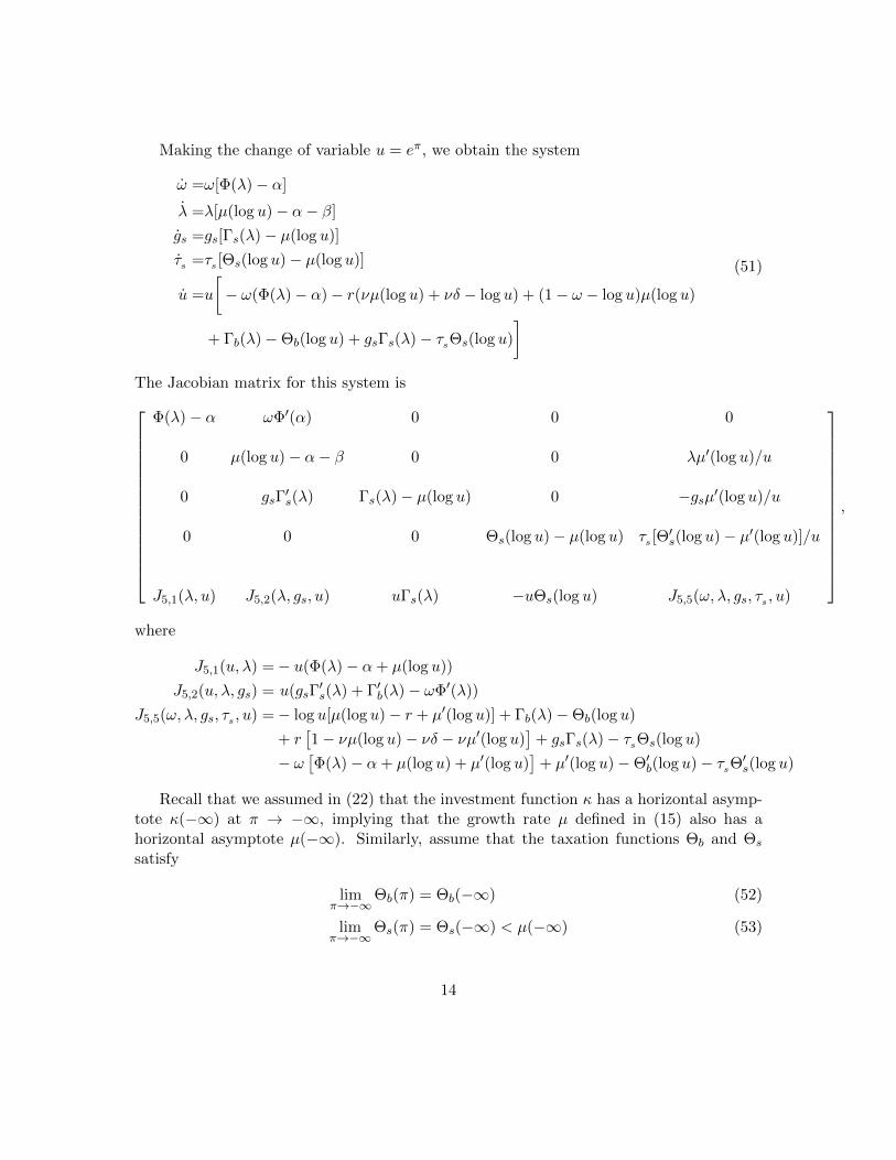
Making the change of variable u = eπ, we obtain the system

ω =ω[Φ(λ)− α]

λ =λ[µ(log u)− α− β]

gs =gs[Γs(λ)− µ(log u)]

τs =τs [Θs(log u)− µ(log u)]

u =u

[− ω(Φ(λ)− α)− r(νµ(log u) + νδ − log u) + (1− ω − log u)µ(log u)

+ Γb(λ)−Θb(log u) + gsΓs(λ)− τsΘs(log u)

](51)

The Jacobian matrix for this system is

Φ(λ)− α ωΦ′(α) 0 0 0

0 µ(log u)− α− β 0 0 λµ′(log u)/u

0 gsΓ′s(λ) Γs(λ)− µ(log u) 0 −gsµ′(log u)/u

0 0 0 Θs(log u)− µ(log u) τs [Θ′s(log u)− µ′(log u)]/u

J5,1(λ, u) J5,2(λ, gs, u) uΓs(λ) −uΘs(log u) J5,5(ω, λ, gs, τs , u)

,

where

J5,1(u, λ) =− u(Φ(λ)− α+ µ(log u))

J5,2(u, λ, gs) = u(gsΓ′s(λ) + Γ′b(λ)− ωΦ′(λ))

J5,5(ω, λ, gs, τs , u) =− log u[µ(log u)− r + µ′(log u)] + Γb(λ)−Θb(log u)

+ r[1− νµ(log u)− νδ − νµ′(log u)

]+ gsΓs(λ)− τsΘs(log u)

− ω[Φ(λ)− α+ µ(log u) + µ′(log u)

]+ µ′(log u)−Θ′b(log u)− τsΘ′s(log u)

Recall that we assumed in (22) that the investment function κ has a horizontal asymp-tote κ(−∞) at π → −∞, implying that the growth rate µ defined in (15) also has ahorizontal asymptote µ(−∞). Similarly, assume that the taxation functions Θb and Θs

satisfy

limπ→−∞

Θb(π) = Θb(−∞) (52)

limπ→−∞

Θs(π) = Θs(−∞) < µ(−∞) (53)

14

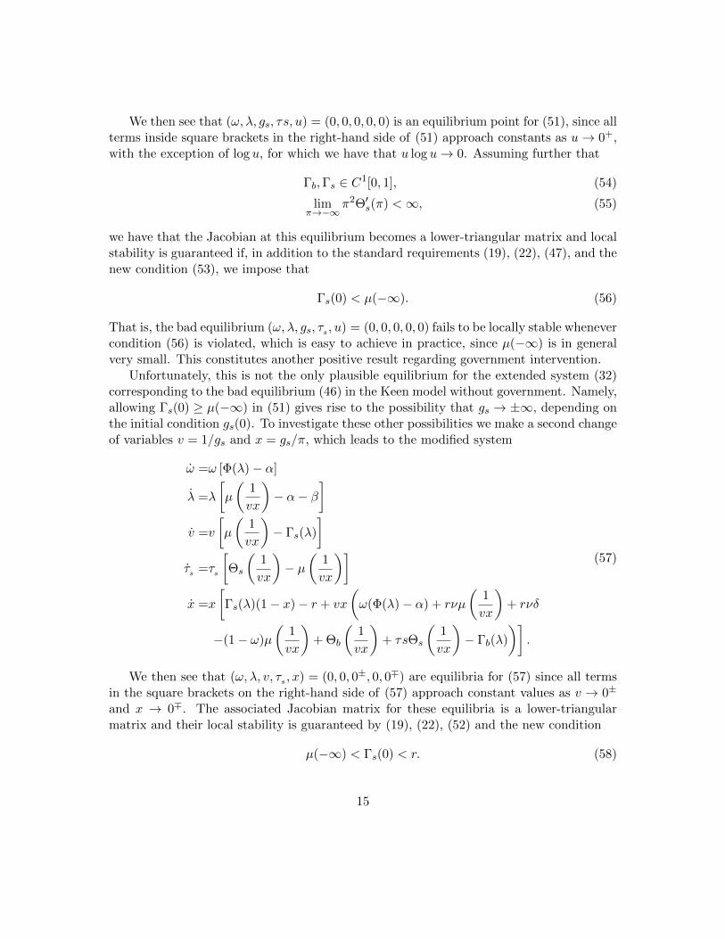
We then see that (ω, λ, gs, τs, u) = (0, 0, 0, 0, 0) is an equilibrium point for (51), since allterms inside square brackets in the right-hand side of (51) approach constants as u→ 0+,with the exception of log u, for which we have that u log u→ 0. Assuming further that

Γb,Γs ∈ C1[0, 1], (54)

limπ→−∞

π2Θ′s(π) <∞, (55)

we have that the Jacobian at this equilibrium becomes a lower-triangular matrix and localstability is guaranteed if, in addition to the standard requirements (19), (22), (47), and thenew condition (53), we impose that

Γs(0) < µ(−∞). (56)

That is, the bad equilibrium (ω, λ, gs, τs , u) = (0, 0, 0, 0, 0) fails to be locally stable whenevercondition (56) is violated, which is easy to achieve in practice, since µ(−∞) is in generalvery small. This constitutes another positive result regarding government intervention.

Unfortunately, this is not the only plausible equilibrium for the extended system (32)corresponding to the bad equilibrium (46) in the Keen model without government. Namely,allowing Γs(0) ≥ µ(−∞) in (51) gives rise to the possibility that gs → ±∞, depending onthe initial condition gs(0). To investigate these other possibilities we make a second changeof variables v = 1/gs and x = gs/π, which leads to the modified system

ω =ω [Φ(λ)− α]

λ =λ

[µ

(1

vx

)− α− β

]v =v

[µ

(1

vx

)− Γs(λ)

]τs =τs

[Θs

(1

vx

)− µ

(1

vx

)]x =x

[Γs(λ)(1− x)− r + vx

(ω(Φ(λ)− α) + rνµ

(1

vx

)+ rνδ

−(1− ω)µ

(1

vx

)+ Θb

(1

vx

)+ τsΘs

(1

vx

)− Γb(λ)

)].

(57)

We then see that (ω, λ, v, τs , x) = (0, 0, 0±, 0, 0∓) are equilibria for (57) since all termsin the square brackets on the right-hand side of (57) approach constant values as v → 0±

and x → 0∓. The associated Jacobian matrix for these equilibria is a lower-triangularmatrix and their local stability is guaranteed by (19), (22), (52) and the new condition

µ(−∞) < Γs(0) < r. (58)

15

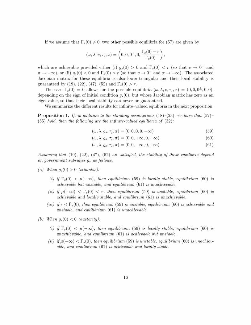
If we assume that Γs(0) 6= 0, two other possible equilibria for (57) are given by

(ω, λ, v, τs , x) =

(0, 0, 0±, 0,

Γs(0)− rΓs(0)

),

which are achievable provided either (i) gs(0) > 0 and Γs(0) < r (so that v → 0+ andπ → −∞), or (ii) gs(0) < 0 and Γs(0) > r (so that v → 0− and π → −∞). The associatedJacobian matrix for these equilibria is also lower-triangular and their local stability isguaranteed by (19), (22), (47), (52) and Γs(0) > r.

The case Γs(0) = 0 allows for the possible equilibria (ω, λ, v, τs , x) = (0, 0, 0±, 0, 0),depending on the sign of initial condition gs(0), but whose Jacobian matrix has zero as aneigenvalue, so that their local stability can never be guaranteed.

We summarize the different results for infinite–valued equilibria in the next proposition.

Proposition 1. If, in addition to the standing assumptions (18)–(23), we have that (52)–(55) hold, then the following are the infinite-valued equilibria of (32):

(ω, λ, gs, τs , π) = (0, 0, 0, 0,−∞) (59)

(ω, λ, gs, τs , π) = (0, 0,+∞, 0,−∞) (60)

(ω, λ, gs, τs , π) = (0, 0,−∞, 0,−∞) (61)

Assuming that (19), (22), (47), (52) are satisfied, the stability of these equilibria dependon government subsidies gs as follows.

(a) When gs(0) > 0 (stimulus):

(i) if Γs(0) < µ(−∞), then equilibrium (59) is locally stable, equilibrium (60) isachievable but unstable, and equilibrium (61) is unachievable.

(ii) if µ(−∞) < Γs(0) < r, then equilibrium (59) is unstable, equilibrium (60) isachievable and locally stable, and equilibrium (61) is unachievable.

(iii) if r < Γs(0), then equilibrium (59) is unstable, equilibrium (60) is achievable andunstable, and equilibrium (61) is unachievable.

(b) When gs(0) < 0 (austerity):

(i) if Γs(0) < µ(−∞), then equilibrium (59) is locally stable, equilibrium (60) isunachievable, and equilibrium (61) is achievable but unstable.

(ii) if µ(−∞) < Γs(0), then equilibrium (59) is unstable, equilibrium (60) is unachiev-able, and equilibrium (61) is achievable and locally stable.

16

In other words, under a stimulus regime (gs(0) > 0), any achievable equilibria withπ → −∞ becomes unstable provided Γs(0) > r. On the other hand, under an austerityregime (gs(0) > 0), there is no value of Γs(0) that eliminates the possibility of local stabilityfrom all achievable equilibria with π → −∞.

4. Persistence Results

In this section we move beyond local equilibrium analysis to establish under whichconditions government intervention can guarantee that the economy as represented bysystem (32) does not reach a state of permanently zero employment. In other words,we establish persistence for the system of differential equations (32) with respect to theemployment λ. The relevant definitions are reviewed in Appendix C, illustrated by thesimple example of the Goodwin model.

As it is typical in persistence analysis, although we are primarily interest in preventingthe crisis situation characterized by π → −∞, our first result eliminates the possibility ofexploding positive profits.

Proposition 2. If τs(0) ≥ 0, and conditions (21),(22) are satisfied, then the system de-scribed by (32) is e−π-UWP, that is, there exists an ε > 0 such that lim supt→∞ e

−π(t) > εfor any initial conditions.

Proof. Showing this consists of demonstrating

lim inft→∞

π(t) < m

for some m ∈ R. We are going to show this by contradiction, so assume that lim inf π > mfor any m, as large (and positive) as we want. We can then find a t0 such that π(t) > mfor all t ≥ t0.

First, we can then bound employment from below since for t ≥ t0 we have

λ/λ = µ(π)− α− β ≥ µ(m)− α− β

which is positive form large enough. That means that λ(t) > λ(t0) exp [(µ(m)− α− β)(t− t0)]for all t > t0.

Consequently, there exists t1 > t0 for which Φ(λ(t1)) > α and thus

ω/ω = Φ(λ)− α

will be positive. We then have that

ω(t) ≥ ω(t1) exp [Φ(λ(t1))− α]

17

Next, for t ≥ t1, the government spending dynamics satisfy

gs/gs = Γs(λ)− µ(π) ≤ Γs(λ(t1))− µ(m)

which can be made negative form large enough. Consequently, |gs(t)| ≤ |gs(t1)| exp [(Γs(λ(t1))− µ(m))(t− t1)]for all t > t0.

Finally, one can choose m big enough such that κ(m) ≥ 0, θb(m) ≥ 0, θs(m) ≥ 0, andµ(m) > r (possible because of (22)), allowing us to find the following bound for π, validfor all t > t1:

π = −ω[Φ(λ)− α]− r(κ(π)− π) + (1− ω − π)µ(π) + Γb(λ)−Θb(π) + gsΓs(λ)− τsΘs(π)

≤ π [r − µ(m)]− ω(t1)e[Φ(λ(t1))−α](t−t1) [Φ(λ(t1))− α] + Cm,

(62)

where Cm = Γb(λ(t0))+(gs(t0))+ Γs(λ(t0)) is a positive constant. Consequently, Gronwall’sinequality gives the following bound, valid for any t > t0

π(t) ≤ π(t1)e−(µ(m)−r)(t−t1) +Cm

µ(m)− r

(1− e−[µ(m)−r](t−t1)

)− ω(t1) [Φ(λ(t1))− α]

[Φ(λ(t1))− α] + [µ(m)− r]

(e[Φ(λ(t1))−α](t−t1) − e−[µ(m)−r](t−t1)

) (63)

From (20), we can choose t1 appropriately such that Φ(λ(t1))−α ≥ µ(+∞)−r and thusthe RHS of (63) converges to −∞ as t increases, which provides us with a contradiction.

Our core results are presented in the next two propositions. We first show that govern-ment intervention can achieve uniformly weak persistence of the functional eπ even whenthe bad equilibrium for the model without government is locally stable.

Proposition 3. Suppose that the structural conditions (18)-(23) and (28)–(29) are satis-fied, along with the local stability condition (47) for the bad equilibrium of the Keen model(14) without government. Assume further that gs(0) > 0 and that condition (53) is satis-fied. Then the model with government (32) is eπ-UWP if either of the following conditionsis satisfied:

(1) Γs(0) > r, or

(2) λΓb(λ) is bounded below as λ→ 0.

18

Proof. We prove it by contradiction. If lim supt→∞ π(t) ≤ −m for any given large m > 0,there exists t0 ≥ 0 such that π(t) ≤ −m for t > t0. From the equation for λ, it follows that

λ(t) ≤ λ(t0)e(t−t0)(µ(−m)−α−β),

for t > t0. Choosing m > 0 large enough so that µ(−m) < α + β (recall condition (22)),we get that for any small ε > 0, there exists t1 > t0 such that λ(t) < ε for t > t1. Fromthe equation for ω, this readily implies that

ω(t) < ω(t1)e(t−t1)(Φ(ε)−α),

for t > t1. Again, we may choose ε > 0 sufficiently small that Φ(ε) < α (recall conditions(18) and (19)). Hence, there exists t2 > t1 > t0 such that ω(t) < ε for t > t2. Finally,condition (53) guarantees that we can choose m large enough such that

Θs(π)− µ(π) < 0, ∀π ≤ −m.

It then follows from the equation for τs that there exists t3 > t2 > t1 > t0 such thatτs(t) < ε for t > t3. In other words, we can bound ω, λ and τs by ε for t large enough.

At this point, we need to consider the hypothesis Γs(0) > r and λΓb(λ) bounded sepa-rately. Assume first that Γs(0) > r. Since Γ is a decreasing function, we can immediatelysee from the equation for gs that

gsgs

= Γs(λ)− µ(π) > Γs(ε)− µ(π),

for t > t1. Moreover, since Γs(0) > r > µ(−∞) (see condition (47)), we can choose ε smallenough and/or m big enough such that Γs(ε) > µ(−m). Accordingly, for any t > s > t1,we have that

gs(t) > gs(s)e(t−s)[Γs(ε)−µ(−m)].

Using the equation for π we have:

π =− ω[Φ(λ)− α]− r[νµ(π) + νδ − π] + (1− ω − π)µ(π) + Γb(λ) + gsΓs(λ)−Θb(π)− τsΘs(π)

=− ω[Φ(λ)− α]− rκ(π) + π(r − µ(π)) + (1− ω)µ(π) + Γb(λ) + gsΓs(λ)−Θb(π)− τsΘs(π)

>− rmax{|κ(−∞)|, |κ(−m)|}+ π(r − µ(−∞))−max{|µ(−∞)|, |µ(−m)|}+ Γb(ε)

+ Γs(ε)gs(t3)e(t−t3)[Γs(ε)−µ(−m)] −Θb(−m)− εmax{|Θs(−∞)|, |Θs(−m)|}=C +Aπ +DeEt

(64)

where C is finite and does not depend on t, A = r−µ(−∞) > 0, D = Γs(ε)gs(t3)e−t3(Γs(ε)−µ(−m)) >0 and E = Γs(ε)− µ(−m) > 0. Consequently, for t > t3, we have that π(t) > y(t), where

19

y(t) is the solution ofy = C +Ay +DeEt, y(t3) = π(t3), (65)

that is,

y(t) = y(t3)eA(t−t3) +C

A

(eA(t−t3) − 1

)+

D

E −AeEt3

(eE(t−t3) − eA(t−t3)

). (66)

At last, since Γs(0) > r, we can choose ε sufficiently small and m sufficiently large suchthat

E −A = Γs(ε)− r + µ(−∞)− µ(−m) > 0,

which leads us to conclude that eEt dominates the solution y(t) when t→∞, that is,

limt→∞

y(t) =D

E −AeEt = +∞.

Yet, since π(t) > y(t) for t > t3, we must have also π(t)t→∞−−−→ +∞, which contradicts the

fact that π(t) ≤ −m for t > t0.Alternatively, assume now that λΓb(λ) is bounded from below as λ → 0. We can still

bound ω, λ and τs by ε for t large enough as before. Moreover, since λΓb(λ) > L for somepositive L as λ→ 0, we now have that Γb(λ) > Γb(λ)λ/ε > L/ε. From the equation for πwe then have

π =− ω[Φ(λ)− α]− r[νµ(π) + νδ − π] + (1− ω − π)µ(π) + Γb(λ) + gsΓs(λ)−Θb(π)− τsΘs(π)

=− ω[Φ(λ)− α]− rκ(π) + π(r − µ(π)) + (1− ω)µ(π) + Γb(λ) + gsΓs(λ)−Θb(π)− τsΘs(π)

>− rmax{|κ(−∞)|, |κ(−m)|}+ π(r − µ(−∞))−max{|µ(−∞)|, |µ(−m)|}+ L/ε

−Θb(−m)− εmax{|Θs(−∞)|, |Θs(−m)|}=C(ε) + Aπ,

(67)

where C can be made arbitrarily large by choosing ε sufficiently small, while A = r −µ(−∞) > 0. Therefore, for t > t3, we have that π(t) ≥ y(t), where y(t) is now the solutionof

y(t) = C + Ay, y(t3) = π(t3),

that is,

y(t) =

(C(ε) + Ay(t3)

)eA(t−t3) − C

A.

We can then choose ε small enough such that C(ε) + Ay(t3) > 0 and hence limt→∞ y(t) =

+∞. But this implies that π(t)t→∞−−−→ +∞, which again contradicts the fact that π(t) ≤ −m

for t > t0.

20

Although profits play a key role in the model, from the point of view of economic policy,arguably the most important variable in (32) is the rate of employment. Our next andfinal result shows that under slightly stronger conditions we can still obtain uniformly weakpersistence with respect to the functional λ itself. Before stating it, define the function

h(x) = −r[νµ(x) + νδ − x] + (1− x)µ(x) + Γb(0)−Θb(x), (68)

and observe that it has the properties:

(i) h(π1) = ω1(α+ β) + Γb(0)− Γb(λ1) > 0,

(ii) limx→±∞

h(x) = −∞, and

(iii) max[h(π)] < +∞.

Proposition 4. Suppose that the structural conditions (18)–(23) and (28)–(29) are satis-fied, along with the local stability condition (47) for the bad equilibrium of the Keen model(14) without government. Assume further that gs(0) > 0 and that condition (53) is satis-fied. Then the system (32) is λ-UWP if either of the following four conditions is satisfied:

(1) τs(0) = 0 and Γs(0) > max{r, α+ β}, or

(2) τs(0) = 0 and λΓb(λ) is bounded below as λ→ 0, or

(3) τs(0) = 0, r < Γs(0) ≤ α+ β, and h(x) > 0 whenever µ(x) ∈ [Γs(0), α+ β], or

(4) Γs(0) > max{r, α+ β}, Θs(−∞) < 0, Θs(π1) < α+ β, and Θs is convex.

Proof. We prove the result by contradiction again. If lim supt→∞ λ(t) ≤ ε for any ε > 0,then there exists t0 > 0 such that λ(t) ≤ ε for t > t0. Since we can always choose ε smallenough so that Φ(ε)− α < 0, it follows from the equation for ω as before that there existst1 > t0 such that ω(t) < ε for all t > t1.

For items (1) and (2), observe that it follows from UWP of eπ obtained in Proposition3 that we can find a large m1 > 0 such that lim supt→∞ π(t) > −m1. In addition, we havethat lim inft→∞ π < µ−1(α+β) = m2, since otherwise λ cannot converge to zero and thereis nothing left to prove. Let m = max{m1,m2}.

If Γs(0) > max{r, α+ β}, we see from the equation for λ that

exp

[∫ t

t1

µ(πs)ds

]<

ε

λ(t1)e(α+β)(t−t1) ∀t > t1,

which implies that

gs(t) >λ(t1)gs(t1)

εexp [(Γs(ε)− (α+ β)) (t− t1)] ∀t > t1

21

In other words, given any large L > 0, provided we choose ε sufficiently small so thatΓs(ε) > α+β, there exists t2 > t1 such that gs(t) > L for t > t2. Alternatively, if λΓb(λ) isbounded below as λ→ 0, given any large L > 0, we can choose ε sufficiently small so thatΓb(λ) > L for λ < ε (since Γb(λ) > L0/λ > L0/ε for some L0 > 0, just choose ε ≤ L0/L).

In either case, we can find ε > 0 small enough and/or t2 > t1 such that

− ω[Φ(λ)− α]− r[νµ(π) + νδ− π] + (1− ω− π)µ(π) + Γb(λ) + gsΓs(λ)−Θb(π) > ε (69)

for all ω ∈ [0, ε], λ ∈ [0, ε], π ∈ [−m,m] and t > t2. Since lim supπ > −m and lim inf π <m, we can find t3 > t2 such that π(t3) ∈ (−m,m), from which it follows from (69) and theequation for π that π(t3) > 0. Furthermore, π(t) > 0 for all t > t3 with π(t) ≤ m. Hence,there exists t4 > t3 such that π(t4) = m and π(t) > m for all t > t4. But this contradictsthe fact lim inf π < m, and UWP of λ follows.

For item (3), we can again find a sufficiently small ε and a sufficiently large t0 > 0 suchthat ω(t) < ε and λ(t) < ε for all t > t0, and

−ω[Φ(λ)− α]− r[νµ(π) + νδ − π] + (1− ω − π)µ(π) + Γb(ε) + gsΓs(ε)−Θb(π) > ε

for all ω ∈ [0, ε], λ ∈ [0, ε] and π in the interval such that Γs(0) ≤ µ(π) ≤ α + β. We usethe fact that Γs(0) > r, which implies eπ −UWP , to obtain that π does enter the interval[−m,m], for some large m ≥ µ−1(α + β)), at some instant t1 > t0. But since π(t) > εwhenever π(t) lies in the interval such that Γs(0) ≤ µ(π) ≤ α+β), this in turn implies that−m < π < µ−1(Γs(0)) for all t > t1, because otherwise π > µ−1(α + β) for all large t andλ(t) could not go to zero. However, µ(π) < Γs(0) for all large t implies that gs(t) can bemade arbitrarily large and we have that (69) holds, which again leads to a contradiction.

The proof of item (4) is presented in Appendix D.

5. Examples

In this section we compare the results obtained for a Keen model without governmentdescribed by (14) with the model with government described by (32) under several differentscenarios. For the basic parameter values we fix the capital-to-output ratio ν, the rate ofproductivity growth α, the rate of population growth β, the depreciation rate δ =, and thereal short-term interest rate on for private debt r at the following values

ν = 3, α = 0.025, β = 0.02, δ = 0.01, r = 0.03.

22

In addition, for the Keen model without government we use the functions

Φ(λ) =φ1

(1− λ)2− φ0 (70)

κ(π) = κ0 + κ1 arctan(κ2π + κ3) (71)

with parameter values given in Appendix E. We can easily verify that all the structuralconditions (18)-(23) are satisfied for these functions. Moreover, we have that

r

[κ′(π1)

ν(π1 − κ(π1) + ν(α+ β))− (α+ β)

]= 0.00515 > 0 (72)

so that (45) is satisfied and the good equilibrium

(ω1, λ1, d1) = (0.83667, 0.96, 0.11111) (73)

is locally stable. Finally, observe that

κ(−∞)

ν− δ = −0.01 < 0.03 = r (74)

so that (47) is satisfied and the bad equilibrium (ω2, λ2, d2) = (0, 0,+∞) is also locallystable. That is, for these parameters, in the absence of government intervention, theeconomy converges to either the good or the bad equilibrium depend on how close to themwe chose the initial conditions.

For the model (32) with government, we use functions

Γb(λ) = γ0(1− λ) (75)

Γs(λ) = γ1 − γ2λγ3 (76)

Θb(π) = θ0 + θ1eθ2π (77)

Θs(π) = θ3 + θ4eθ5π (78)

ge(π, λ) = (1− κ(π))(1− λ)γ4 (79)

with parameter values given in Appendix E. Observe that we specified government expen-ditures directly through the function ge(π, λ) above, instead of equivalently defining it asthe solution of (38).

We can again easily verify that the structural conditions (52)–(55) are satisfied. Wecan also verify that conditions (B.4)–(B.7) are also satisfied, so that the good equilibrium

(ω, λ, gs, τs , π) = (ω1, λ1, 0, 0, π1) = (0.76067, 0.96, 0, 0, 0.16)

is locally stable. Moreover, we can verify that the conditions for stability of the other

23

finite-valued equilibria in (50) are easily violated for our choice of parameters, so that noneof them is locally stable.

As we have seen in Proposition 1, the stability of the infinite-valued equilibria in thepresence of government intervention depends crucially on the parameter Γs(0) = γ1 cor-responding to the maximum value of the discretionary subsidy function above. In whatfollows we set

γ1 =

{0.02 for a timid government,

0.20 for a responsive government.(80)

It then follows from item (a) of Proposition 1 that in a stimulus regime, namely for initialconditions with gs(0) > 0, equilibrium (59) is unstable in either case, whereas equilibrium(60) is stable in the case of a timid government but unstable in the case of a responsivegovernment. On the other hand, it follows from item (b) that in an austerity regime, thatis for initial conditions with gs(0) < 0, equilibrium (61) is locally stable in either case.

Moving to the persistence results in Section 4, observe that condition (1) of Proposition3 is satisfied in the case of a responsive government, but that neither conditions in thisproposition are satisfied in the case of a timid government. As a result, provided gs(0) > 0,the responsive government above ensures uniformly weakly persistence with respect to eπ,but the timid government does not.

Similarly, we can verify that condition (4) of Proposition 4 is satisfied by our responsivegovernment even when τs(0) > 0, but none of the conditions in this proposition are satisfiedby the timid government. Consequently, provided gs(0) > 0, the responsive governmentabove ensures uniformly weakly persistence with respect to λ, but the timid governmentdoes not.

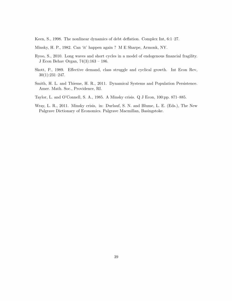
We illustrate these results in the next six figures. Choosing benign initial conditions,that is to say, high wage share (90% of GDP), high employment rate (90%), and lowprivate debt (10% of GDP), we see in Figure 1 that the economy eventually converges tothe corresponding good equilibrium with or without government intervention, even in thecase of a timid government.

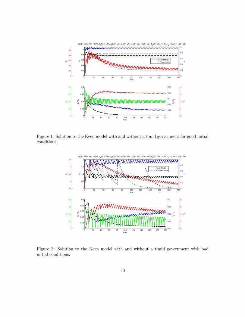
As we move to worse initial conditions, that is lower wage share (75% of GDP), loweremployment rate (80%), and higher private debt (50% of GDP), we see in Figure 2 thatthe “free economy” represented by the model without government eventually collapses tothe bad equilibrium of zero wage share, zero employment and infinite private debt, whereasthe model with a timid government is more robust and eventually converges to the goodequilibrium.

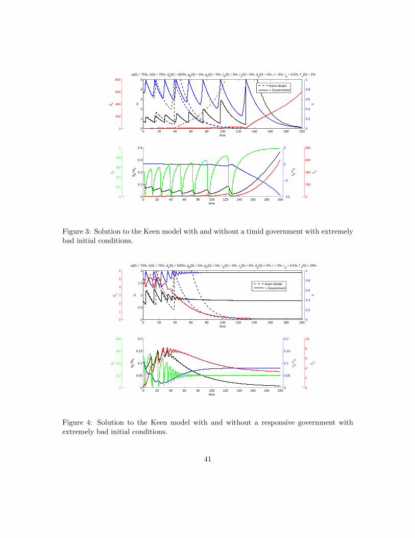
A timid government, however, is not capable of saving the economy from a crash ifthe initial conditions are too extreme, for example a low wage share (75% of GDP), lowemployment rate (75%) and extremely high level of private debt (500% of GDP), as shownin Figure 3. On the other hand, a responsive government, effectively brings the economyfrom the severe crisis induced by this extremely bad initial conditions, as shown in Figure4).

24

Additionaly, the effects of austerity measures are exemplified in Figures 5 and 6. For ahealthy initial state, we see that the transient period suffers from the negative spending,compared to a positive stimulus, without any long term consequences. Once we push theinitial state further away from the good equilibrium, we can immediately verify the disas-trous consequences of austerity: the government focuses so much on reducing public debtthat it throws the economy into recession.

6. Concluding Remarks

We proposed a macroeconomic model in which government intervention has a clearpositive effect in preventing a crises characterized by collapsing employment rates. In theabsence of government, the dynamics of the model is primarily driven by the investmentdecisions of capitalists based on profit levels: high profits lead to high investment andeconomic expansion financed by increasing private debt levels. This can lead either to anequilibrium with a finite private debt to output ratio or to another equilibrium where thisratio becomes infinite while the wage share and the employment rate both collapse to zero.Government intervention prevents this outcome by putting a floor under profit levels.

The model without government is essentially that proposed in Keen (1995) and furtheranalyzed in Grasselli and Costa Lima (2012). However, the extended model with gov-ernment presented in Keen (1995) does not differentiate between direct subsidies to firmsand government expenditures in goods and services. The distinction is important becausethe former affects the profit share π in (30), whereas the latter influences it only directlythrough a increased output. This was later partially remedied in Keen (1998), where gov-ernment spending is restricted to subsidies, resulting in government debt not fully reflectingall government transactions. By contrast, we explicitly model both government subsidiesin (26) and expenditures in (37). Expectedly, because of their direct appearance in theprofit equation (30), government subsidies to firms play a far more important role in themodel than government expenditures on goods and services. Somewhat unexpectedly, theactual functional form of government expenditures can be very general without altering theresults at all: the only requirement in (37) is that is cannot depend explicitly on the levelof government debt. This relative unimportance of government consumption is partiallyexplained by the fact that, in this formulation of the model, consumption by households isan accommodating variable determined by equation (41). It is likely that, in more generalformulations with an independent specification of household saving propensity, governmentconsumption plays a more important role in maintaining aggregate demand, with the over-all role of government intervention in preventing a collapse in profits remaining the sameas in this paper.

Our first positive result is the local stability conditions for all finite-valued equilibriaassociated with zero wage shares in (50) are easily violated. But this was also the case forboth the Keen model without government and for its predecessor, the Goodwin model. The

25

next result, however, is truly novel: all equilibria with zero wage share and employmentarising from infinitely negative profit shares can be made either unstable or unachievableby moderately high government subsidies at very low employment. This is in contrastwith the situation without government, where the corresponding bad equilibrium is locallystable for typical parameter values.

The core persistence results of Section 4 are much stronger: government intervention,in the form of responsive enough subsidy and taxation policies, prevent the economy fromremaining permanently at arbitrarily low levels of employment regardless of the initialconditions of the system. It may be that stabilizing an unstable economy is too tall anorder for the government sector, but destabilizing a stable crises is perfectly possible.

Acknowledgements: We thank Carl Chiarella, Steve Keen, and Peter Skott for insight-ful discussions and numerous suggestions, as well as the participants of the Research inOptions Conference, Angra dos Reis, Brazil (December 2012), the Finance Seminars, Uni-versity of Technology Sydney (February 2013), and the Economic Theory Seminar, Uni-versity of Massachusetts at Amherst (April 2013), where this work was presented. Thisresearch received partial financial support from the Institute for New Economic Thinking(Grant INO13-00011), the Natural Sciences and Engineering Research Council of Canada(Discovery Grants), and the Canada Research Chairs Program.

Appendix A. Other finite-valued equilibria with government

1. Take ω2 = 0 and π2 = π1 so that ω = λ = 0. In this case, discarding the structuralcoincidence Θs(π1) = α+ β, the only way to obtain τs = 0 is to set τ s2 = 0. For theremaining variables we define

λ2 = Γ−1s (α+ β) (A.1)

so that gs = 0 and

gs2 =Θb(π1)− Γb(λ2)

α+ β+r(νµ(π1) + νδ − π1)

α+ β− (1− π1) (A.2)

so that π = 0.

2. Take ω3 = τ s3 = 0 and π3 = π1 and so that ω = λ = τs = 0 as before. In additiontake gs3 = 0 so that gs = 0. To obtain π = 0 define

λ3 = Γ−1b (r (νµ(π1) + νδ − π1)− (1− π1) (α+ β) + Θb (π1)) . (A.3)

3. Take ω4 = λ4 = gs4 = τ s4 = 0 so that ω = λ = gs = τs = 0. To obtain π = 0 define

26

π4 as the solution of

− r(νµ(π) + νδ − π) + (1− π)µ(π) + Γb(0)−Θb(π) = 0. (A.4)

4. Take ω5 = λ5 = gs5 = 0 so that ω = λ = gs = 0. To obtain τs = 0 define π5 as thesolution of

Θs(π)− µ(π) = 0. (A.5)

Finally, to obtain π = 0 set

τ s5 =−r(νµ(π5) + νδ − π5) + (1− π5)Θs(π5) + Γb(0)−Θb(π5)

Θs(π5). (A.6)

5. Take ω6 = λ6 = 0 so that ω = λ = 0. To obtain gs = 0, define

π6 = µ−1 (Γs(0)) . (A.7)

Provided we discard again the structural coincidence Θs(π6) = Γs(0), this meansthat to obtain τs = 0 we must set τ s6 = 0. For the remaining variable we take

gs6 =r(νµ(π6) + νδ − π6)− (1− π6)Γs(0)− Γb(0) + Θb(π6)

Γs(0)(A.8)

so that π = 0.

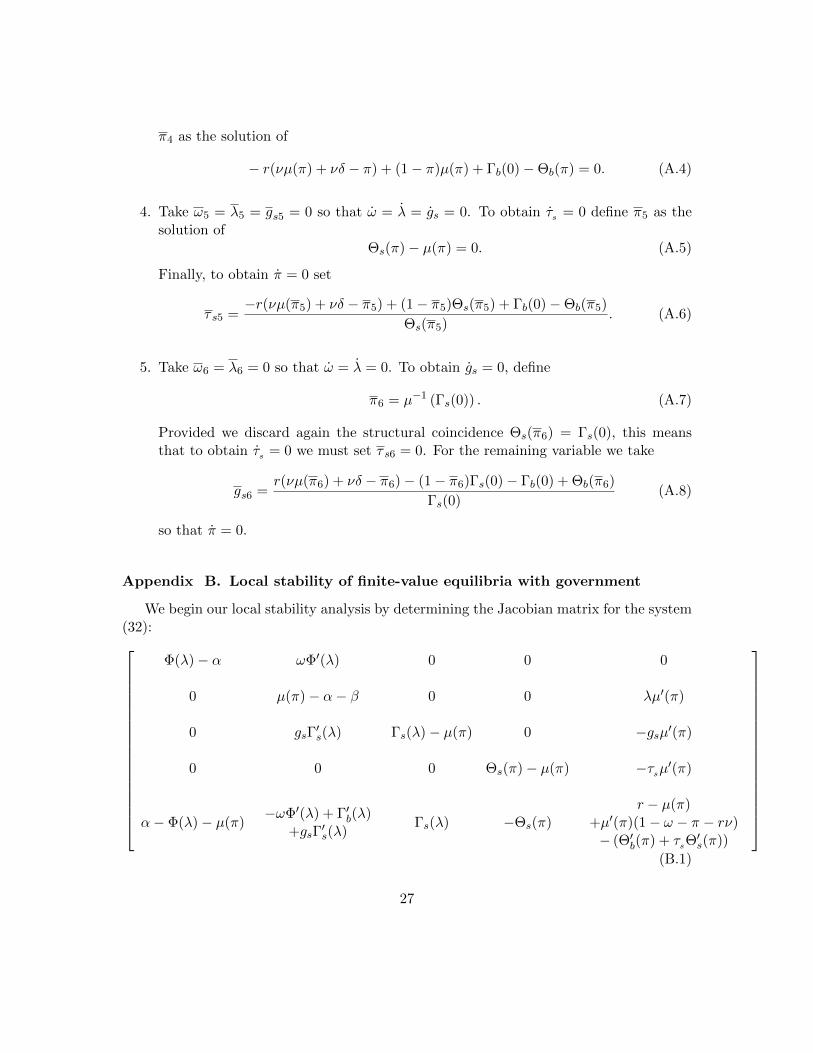
Appendix B. Local stability of finite-value equilibria with government

We begin our local stability analysis by determining the Jacobian matrix for the system(32):

Φ(λ)− α ωΦ′(λ) 0 0 0

0 µ(π)− α− β 0 0 λµ′(π)

0 gsΓ′s(λ) Γs(λ)− µ(π) 0 −gsµ′(π)

0 0 0 Θs(π)− µ(π) −τsµ′(π)

α− Φ(λ)− µ(π)−ωΦ′(λ) + Γ′b(λ)

+gsΓ′s(λ)

Γs(λ) −Θs(π)r − µ(π)

+µ′(π)(1− ω − π − rν)− (Θ′b(π) + τsΘ

′s(π))

(B.1)

27

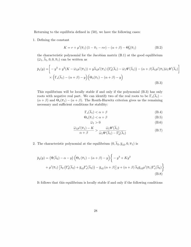
Returning to the equilibria defined in (50), we have the following cases:

1. Defining the constant

K = r + µ′(π1) (1− π1 − rν)− (α+ β)−Θ′b(π1) (B.2)

the characteristic polynomial for the Jacobian matrix (B.1) at the good equilibrium(ω1, λ1, 0, 0, π1) can be written as

p1(y) =

[− y3 + y2(K − ω1µ

′(π1)) + yλ1µ′(π1)

(Γ′b(λ1)− ω1Φ′(λ1)

)− (α+ β)λ1µ

′(π1)ω1Φ′(λ1)

]×(

Γs(λ1)− (α+ β)− y)(

Θs(π1)− (α+ β)− y)

(B.3)

This equilibrium will be locally stable if and only if the polynomial (B.3) has onlyroots with negative real part. We can identify two of the real roots to be Γs(λ1) −(α + β) and Θs(π1)− (α + β). The Routh-Hurwitz criterion gives us the remainingnecessary and sufficient conditions for stability:

Γs(λ1) < α+ β (B.4)

Θs(π1) < α+ β (B.5)

ω1 > 0 (B.6)

ω1µ′(π1)−Kα+ β

>ω1Φ′(λ1)

ω1Φ′(λ1)− Γ′b(λ1)(B.7)

2. The characteristic polynomial at the equilibrium (0, λ2, gs2, 0, π1) is

p2(y) =(Φ(λ2)− α− y

) (Θs (π1)− (α+ β)− y

){− y3 +Ky2

+ µ′(π1)[λ2

(Γ′b(λ2) + gs2Γ′s(λ2)

)− gs2 (α+ β)

]y + (α+ β)λ2gs2µ

′(π1)Γ′s(λ2)

}(B.8)

It follows that this equilibrium is locally stable if and only if the following conditions

28

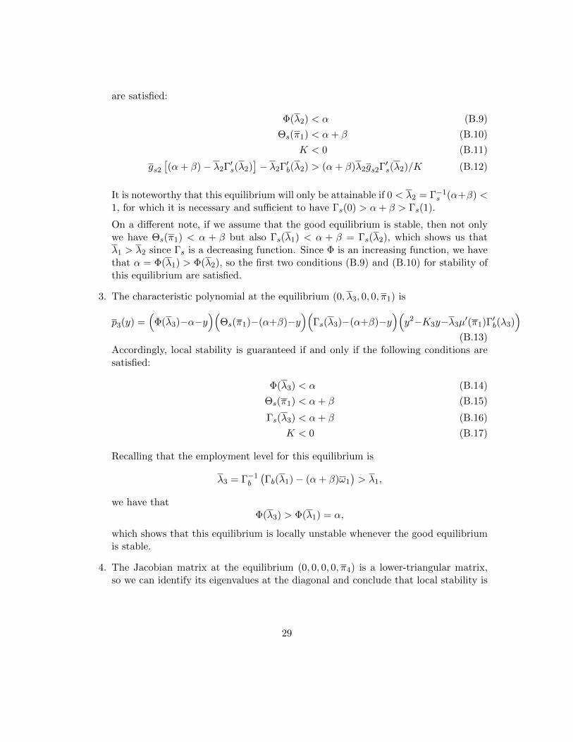
are satisfied:

Φ(λ2) < α (B.9)

Θs(π1) < α+ β (B.10)

K < 0 (B.11)

gs2[(α+ β)− λ2Γ′s(λ2)

]− λ2Γ′b(λ2) > (α+ β)λ2gs2Γ′s(λ2)/K (B.12)

It is noteworthy that this equilibrium will only be attainable if 0 < λ2 = Γ−1s (α+β) <

1, for which it is necessary and sufficient to have Γs(0) > α+ β > Γs(1).

On a different note, if we assume that the good equilibrium is stable, then not onlywe have Θs(π1) < α + β but also Γs(λ1) < α + β = Γs(λ2), which shows us thatλ1 > λ2 since Γs is a decreasing function. Since Φ is an increasing function, we havethat α = Φ(λ1) > Φ(λ2), so the first two conditions (B.9) and (B.10) for stability ofthis equilibrium are satisfied.

3. The characteristic polynomial at the equilibrium (0, λ3, 0, 0, π1) is

p3(y) =(

Φ(λ3)−α−y)(

Θs(π1)−(α+β)−y)(

Γs(λ3)−(α+β)−y)(y2−K3y−λ3µ

′(π1)Γ′b(λ3))

(B.13)Accordingly, local stability is guaranteed if and only if the following conditions aresatisfied:

Φ(λ3) < α (B.14)

Θs(π1) < α+ β (B.15)

Γs(λ3) < α+ β (B.16)

K < 0 (B.17)

Recalling that the employment level for this equilibrium is

λ3 = Γ−1b

(Γb(λ1)− (α+ β)ω1

)> λ1,

we have thatΦ(λ3) > Φ(λ1) = α,

which shows that this equilibrium is locally unstable whenever the good equilibriumis stable.

4. The Jacobian matrix at the equilibrium (0, 0, 0, 0, π4) is a lower-triangular matrix,so we can identify its eigenvalues at the diagonal and conclude that local stability is

29

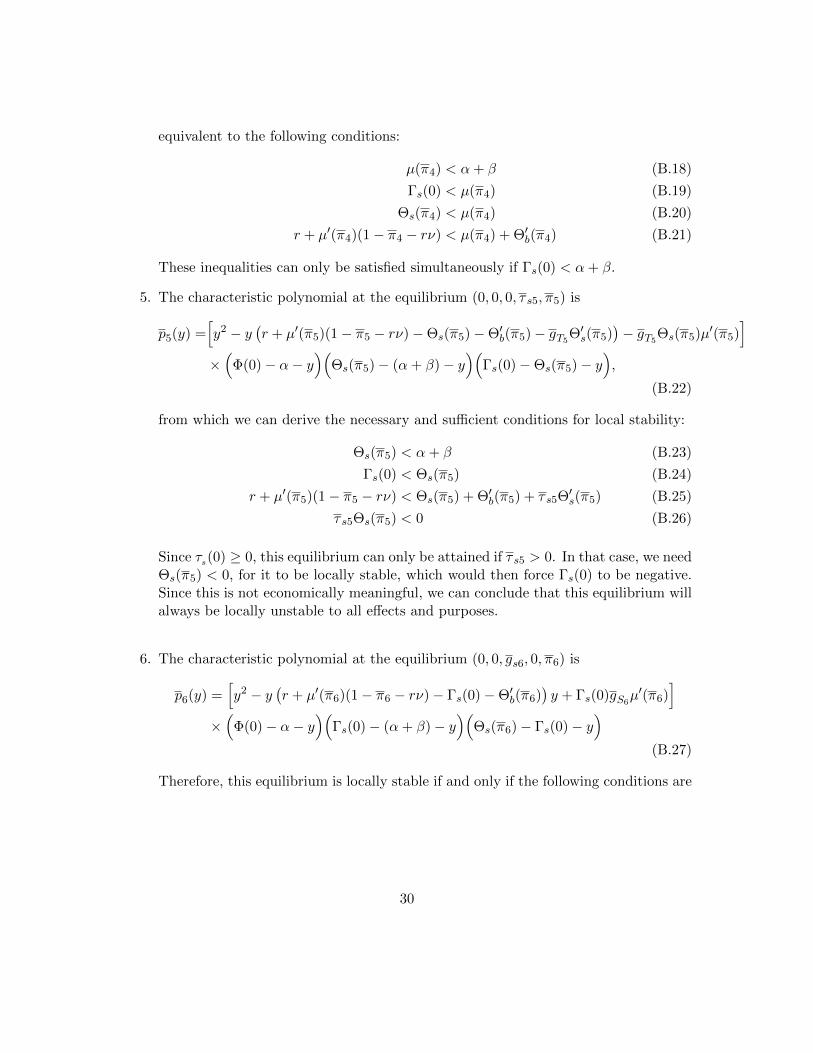
equivalent to the following conditions:

µ(π4) < α+ β (B.18)

Γs(0) < µ(π4) (B.19)

Θs(π4) < µ(π4) (B.20)

r + µ′(π4)(1− π4 − rν) < µ(π4) + Θ′b(π4) (B.21)

These inequalities can only be satisfied simultaneously if Γs(0) < α+ β.

5. The characteristic polynomial at the equilibrium (0, 0, 0, τ s5, π5) is

p5(y) =[y2 − y

(r + µ′(π5)(1− π5 − rν)−Θs(π5)−Θ′b(π5)− gT5Θ′s(π5)

)− gT5Θs(π5)µ′(π5)

]×(

Φ(0)− α− y)(

Θs(π5)− (α+ β)− y)(

Γs(0)−Θs(π5)− y),

(B.22)

from which we can derive the necessary and sufficient conditions for local stability:

Θs(π5) < α+ β (B.23)

Γs(0) < Θs(π5) (B.24)

r + µ′(π5)(1− π5 − rν) < Θs(π5) + Θ′b(π5) + τ s5Θ′s(π5) (B.25)

τ s5Θs(π5) < 0 (B.26)

Since τs(0) ≥ 0, this equilibrium can only be attained if τ s5 > 0. In that case, we needΘs(π5) < 0, for it to be locally stable, which would then force Γs(0) to be negative.Since this is not economically meaningful, we can conclude that this equilibrium willalways be locally unstable to all effects and purposes.

6. The characteristic polynomial at the equilibrium (0, 0, gs6, 0, π6) is

p6(y) =[y2 − y

(r + µ′(π6)(1− π6 − rν)− Γs(0)−Θ′b(π6)

)y + Γs(0)gS6

µ′(π6)]

×(

Φ(0)− α− y)(

Γs(0)− (α+ β)− y)(

Θs(π6)− Γs(0)− y)

(B.27)

Therefore, this equilibrium is locally stable if and only if the following conditions are

30

satisfied:

Γs(0) < α+ β (B.28)

Θs(π6) < Γs(0) (B.29)

r + µ′(π6)(1− π6 − rν) < Γs(0) + Θ′b(π6) (B.30)

gs6Γs(0) > 0 (B.31)

Appendix C. Persistence definitions and examples

We start with a few standard definitions. Let Φ(t, x) : R+ ×X → X be the semiflowgenerated by a differential system with initial values x ∈ X. For a nonnegative functionalρ from X to R+, we say

• Φ is ρ – uniformly strongly persistent (USP) if there exists an ε > 0 such thatlim inft→∞ ρ(Φ(t, x)) > ε for any x ∈ X with ρ(x) > 0.

• Φ is ρ – uniformly weakly persistent (UWP) if there exists an ε > 0 such thatlim supt→∞ ρ(Φ(t, x)) > ε for any x ∈ X with ρ(x) > 0.

• Φ is ρ – strongly persistent (SP) if lim inft→∞ ρ(Φ(t, x)) > 0 for any x ∈ X withρ(x) > 0.

• Φ is ρ – weakly persistent (WP) if lim supt→∞ ρ(Φ(t, x)) > 0 for any x ∈ X withρ(x) > 0.

As an example, consider the well known Goodwin (1967) obtained as a special case of(14) with κ(x) = x and d = 0:

ω = ω [Φ(λ)− α]

λ = λ

[1− ων− δ − (α+ β)

](C.1)

As it is well known (see Grasselli and Costa Lima (2012) and references therein), thesolution of (C.1) passing through the initial condition (ω0, λ0) satisfies the equation(

1

ν− α− β − δ

)log

ω

ω0− 1

ν(ω − ω0) = −α log

λ

λ0+

∫ λ

λ0

Φ(s)

sds. (C.2)

The closed periodic orbits implied by this equation are shown in Figure C.7. Recallingthat π = 1 − ω for this model, observe that ω remains bounded on each orbit, so thatlim inft→∞ exp(1 − ω) > 0 and the system is eπ – strongly persistent. However, since the

31

bound on ω can be made arbitrarily large by changing the initial conditions, we see thatthe system is not eπ – uniformly strongly persistent. Finally, we see in Figure C.7 that ωbecomes smaller than the equilibrium value

ω = 1− ν(α+ β + δ) (C.3)

infinitely often, regardless of the initial conditions. Therefore, taking ε < exp(1−ω) showsthat the system is eπ – uniformly weakly persistent. Exactly the same arguments showthat the Goodwin model (C.1) is λ–SP, λ–UWP, but not λ–USP.

For the Keen model without government intervention defined in (14) the situation isless satisfactory. Whenever the conditions for local stability of the bad equilibrium (46)are satisfied, we cannot have either λ or eπ persistence of any form, since initial conditionssufficiently close to the bad equilibrium will necessarily lead to λ = eπ = 0 asymptotically.

Appendix D. Proof of Proposition 4 - item (4)

For item (4) of Proposition 4, let τs(0) > 0, since otherwise this reduces to item (1)and there is nothing to prove. We start by defining v = τs

gsand observing that

v

v= Θs(π)− Γs(λ).

We can write π in terms of v and g (defined in (68)) as

π = −ω[Φ(λ)− α]− ωµ(π) + g(π) + Γb(λ)− Γb(0) + gs [Γs(λ)− vΘs(π)] (D.1)

Let us now choose ε small enough such that Φ(ε) < α, Γs(ε) > α+ β and

Γs(ε)Γs(ε)− 2ε

Γs(0) + 2ε> Θs(π1), (D.2)

which is possible because by hypothesis Θs(π1) < α+ β < Γs(0).There must then exists some t0 > 0 such that λ(t) ≤ ε and ω(t) ≤ ε for all t > t0. From

UWP of eπ, we can find m > 0 large enough such that lim supπ > −m and lim inf π < m.Let us choose m large enough such that −m < Θ−1

s (0) and

Γs(ε)− 2ε

Γs(0) + 2εΘs(m) > Γs(0).

Using the equations for λ and gs, it is straightforward to see that

εgs(t) > gs(t0)λ(t0)e[Γs(ε)−(α+β)](t−t0) ∀t > t0, (D.3)

which grows exponentially since Γs(ε) > α+β. Accordingly, we can find t1 > t0 such that:

32

(i) εgs(t) > ε [α− Φ(0)− µ(−∞)] + maxπ∈R[g(π)] and

(ii) εgs(t) > εµ(m) + maxπ∈[−m,m] |g(π)|+ Γb(0)− Γb(ε) and

(iii) εgs(t) >Γs(0)2

4Θ′s(−m) and

(iv) εgs(t) >Θs(m)[Θs(m)−Γs(ε)]

Θ′s(−m)

for all t > t1. As a result, π can be globally bounded from above by

π < ε [α− Φ(0)− µ(−∞)] + max[g(π)] + gs[Γs(0)− vΘs(π)] (D.4)

< gs [ε+ Γs(0)− vΘs(π)] (D.5)

for all t > t1. In addition, we have that π can be locally bounded from below by

π > −εµ(m)− maxπ∈[−m,m]

|g(π)|+ Γb(ε)− Γb(0) + gs[Γs(ε)− vΘs(π)] (D.6)

> gs [−ε+ Γs(ε)− vΘs(π)] (D.7)

for all t > t1 such that π(t) ∈ [−m,m]. We can therefore conclude that, for t > t1 andπ(t) ∈ [−m,m], if vΘs(π) ≥ Γs(0) + 2ε, then π ≤ −εgs and if vΘs(π) ≤ Γs(ε) − 2ε, thenπ ≥ εgs.

Moreover, we can globally bound v from both sides as

Θs(π)− Γs(0) <v

v< Θs(π)− Γs(ε), (D.8)

so that π < Θ−1 (Γs(ε)) implies v < 0, whereas π > Θ−1 (Γs(0)) implies v > 0.Observe further that lim inf π ≥ Θ−1

s (0), because when π ∈ [−m,Θ−1s (0)] the lower

bound for π becomes strictly positive for t > t1, forcing π to grow higher than Θ−1s (0). We

can therefore assume, without loss of generality, that 0 ≤ Θs(π1) ≤ Θs(m), since otherwisewe would be done (π1 = µ−1(α+β) would be smaller than the lower bound of the lim inf πand λ could not go to zero).

We shall now define the following regions, contained in [θ−1s (0),m] × R+ (see Figure

D.8):

• V :={

(π, v) ∈ [Θ−1s (0),m]×

[Γs(0)+2ε

Θs(m) ,+∞)

: Γs(ε)− 2ε ≤ vΘs(π) ≤ Γs(0) + 2ε}

;

• S :={

(π, v) ∈ [Θ−1s (0),m]×

[Γs(ε)−2ε

Γs(0) , Γs(0)+2εΓ2(ε)

]: Γs(ε)− 2ε ≤ vΘs(π) ≤ Γs(0) + 2ε

};

33

• P :=(Θ−1s (Γs(0)) ,m

]×(

0, Γs(0)+2εΘs(m)

)With the bounds on π and v obtained above, one can observe the following (valid for

t > t1):

(i) The flow through v = Γs(0)+2εΘs(π) goes inwards the region V . To see this, define the

outward normal vector

~nu :=

{[Γs(0) + 2ε] Θ′s(π)

Θ2s(π)

}and notice that the flow going through the curve obeys

~nu ·{πv

}= [Γs(0) + 2ε] Θ′s(π)π + Θ2

s(π)v [Θs(π)− Γs(λ)]

= [Γs(0) + 2ε] Θ′s(π)π + Θ2s(π)

Γs(0) + 2ε

Θs(π)[Θs(π)− Γs(λ)]

= [Γs(0) + 2ε]{

Θ′s(π)π + Θs(π) [Θs(π)− Γs(λ)]}

≤ [Γs(0) + 2ε]{−εΘ′s(π)gs + Θs(π) [Θs(π)− Γs(ε)]

}< [Γs(0) + 2ε]

{−Θ′s(π)

Θs(m) [Θs(m)− Γs(ε)]

Θ′s(−m)+ Θs(m) [Θs(m)− Γs(ε)]

}< 0

(D.9)

(ii) the flow through v = Γs(ε)−2εΘs(π) also goes inwards the region V . To see this, define the

outward normal vector

~nl := −{

[Γs(ε)− 2ε] Θ′s(π)Θ2s(π)

}which yields

~nl ·{πv

}= − [Γs(ε)− 2ε]

{Θ′s(π)π + Θs(π) [Θs(π)− Γs(λ)]

}≤ − [Γs(ε)− 2ε]

{εΘ′s(π)gs + Θs(π) [Θs(π)− Γs(0)]

}< − [Γs(ε)− 2ε]

{Θ′s(π)

Γ2s(0)

4Θ′s(−m)− Γ2

s(0)

4

}< 0

(D.10)

34

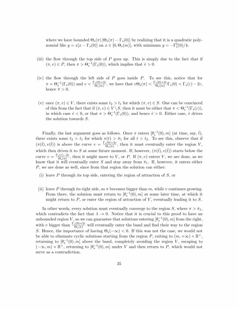
where we have bounded Θs(π) [Θs(π)− Γs(0)] by realizing that it is a quadratic poly-nomial like y = x[x− Γs(0)] on x ∈ [0,Θs(m)], with minimum y = −Γ2

s(0)/4.

(iii) the flow through the top side of P goes up. This is simply due to the fact that if(π, v) ∈ P , then π > Θ−1

s (Γs(0)), which implies that v > 0.

(iv) the flow through the left side of P goes inside P . To see this, notice that for

π = Θ−1s (Γs(0)) and v < Γs(0)+2ε

Θs(m) , we have that vΘs(π) < Γs(0)+2εΘs(m) Γs(0) < Γs(ε)− 2ε,

hence π > 0.

(v) once (π, v) ∈ V , there exists some t2 > t1 for which (π, v) ∈ S. One can be convincedof this from the fact that if (π, v) ∈ V \S, then it must be either that π < Θ−1

s (Γs(ε)),in which case v < 0, or that π > Θ−1

s (Γs(0)), and hence v > 0. Either case, v drivesthe solution towards S.

Finally, the last argument goes as follows. Once π enters [θ−1s (0),m] (at time, say, t),

there exists some t2 > t1 for which π(t) > π1 for all t > t2. To see this, observe that if

(π(t), v(t)) is above the curve v = Γs(0)+2εΘs(π) , then it must eventually enter the region V ,

which then drives it to S at some future moment. If, however, (π(t), v(t)) starts below the

curve v = Γs(ε)−2εΘs(π) , then it might move to V , or P . If (π, v) enters V , we are done, as we

know that it will eventually enter S and stay away from π1. If, however, it enters eitherP , we are done as well, since from that region the solution can either:

(i) leave P through its top side, entering the region of attraction of S, or

(ii) leave P through its right side, so π becomes bigger than m, while v continues growing.From there, the solution must return to [θ−1

s (0),m] at some later time, at which itmight return to P , or enter the region of attraction of V , eventually leading it to S.

In other words, every solution must eventually converge to the region S, where π > π1,which contradicts the fact that λ → 0. Notice that it is crucial to this proof to have anunbounded region V , so we can guarantee that solutions entering [θ−1

s (0),m] from the right,

with v bigger than Γs(0)+2εΘs(π) will eventually enter the band and find their way to the region

S. Hence, the importance of having Θs(−∞) < 0. If this was not the case, we would notbe able to eliminate cyclic solutions starting from the region P , exiting to (m,+∞)×R+,returning to [θ−1

s (0),m] above the band, completely avoiding the region V , escaping to(−∞,m) × R+, returning to [θ−1

s (0),m] under V and then return to P , which would notserve as a contradiction.

35

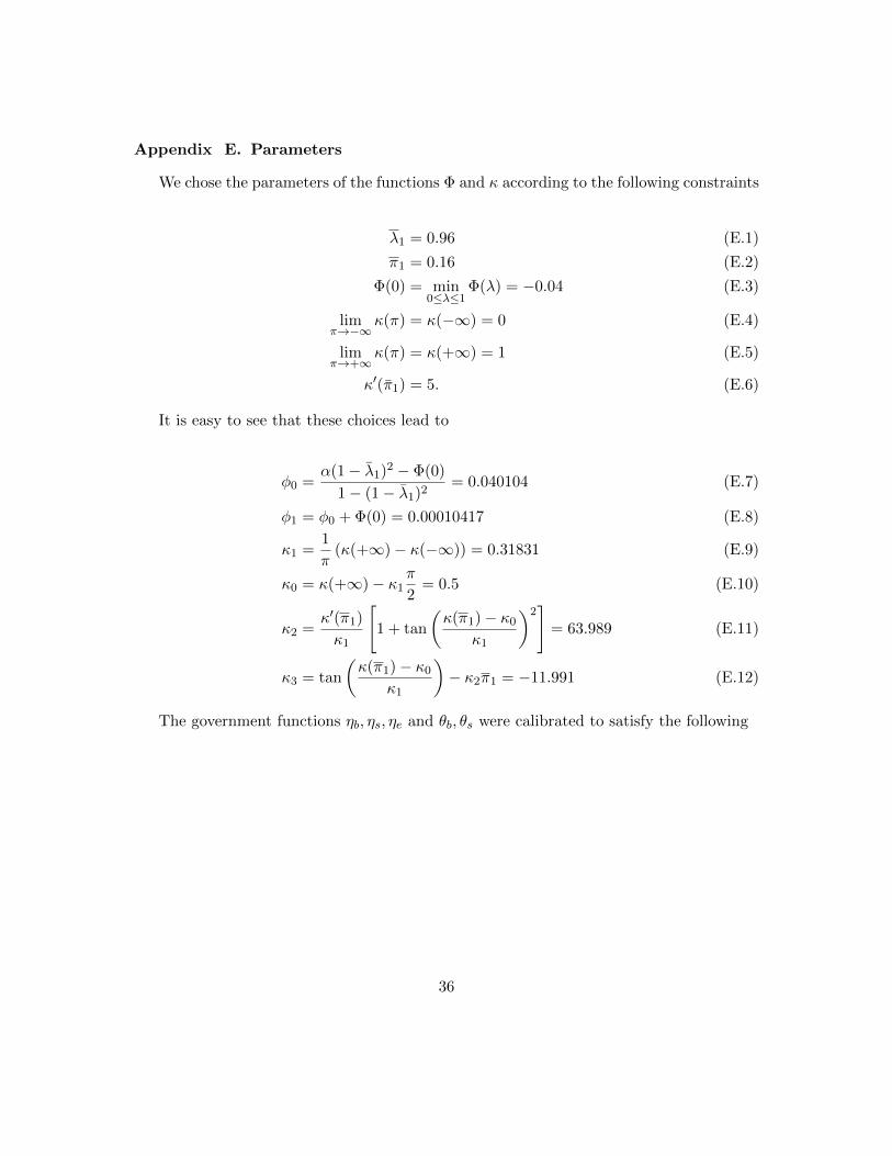
Appendix E. Parameters

We chose the parameters of the functions Φ and κ according to the following constraints

λ1 = 0.96 (E.1)

π1 = 0.16 (E.2)

Φ(0) = min0≤λ≤1

Φ(λ) = −0.04 (E.3)

limπ→−∞

κ(π) = κ(−∞) = 0 (E.4)

limπ→+∞

κ(π) = κ(+∞) = 1 (E.5)

κ′(π1) = 5. (E.6)

It is easy to see that these choices lead to

φ0 =α(1− λ1)2 − Φ(0)

1− (1− λ1)2= 0.040104 (E.7)

φ1 = φ0 + Φ(0) = 0.00010417 (E.8)

κ1 =1

π(κ(+∞)− κ(−∞)) = 0.31831 (E.9)

κ0 = κ(+∞)− κ1π

2= 0.5 (E.10)

κ2 =κ′(π1)

κ1

[1 + tan

(κ(π1)− κ0

κ1

)2]

= 63.989 (E.11)

κ3 = tan

(κ(π1)− κ0

κ1

)− κ2π1 = −11.991 (E.12)

The government functions ηb, ηs, ηe and θb, θs were calibrated to satisfy the following

36

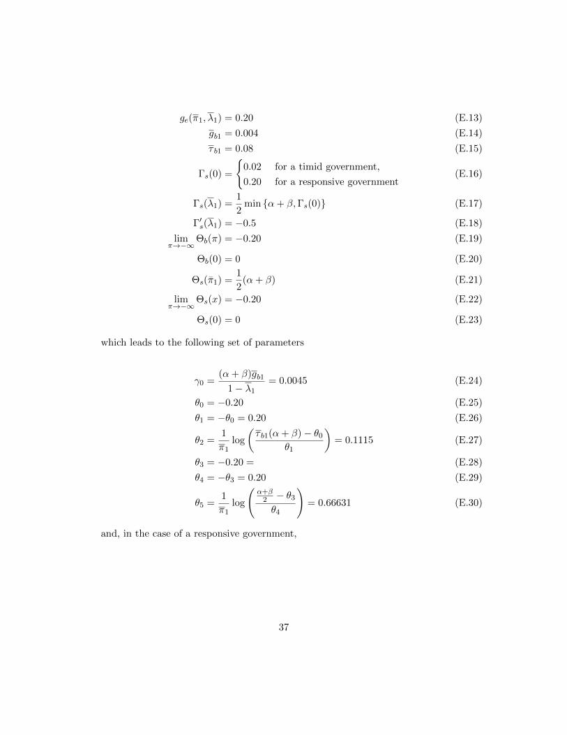
ge(π1, λ1) = 0.20 (E.13)

gb1 = 0.004 (E.14)

τ b1 = 0.08 (E.15)

Γs(0) =

{0.02 for a timid government,

0.20 for a responsive government(E.16)

Γs(λ1) =1

2min {α+ β,Γs(0)} (E.17)

Γ′s(λ1) = −0.5 (E.18)

limπ→−∞

Θb(π) = −0.20 (E.19)

Θb(0) = 0 (E.20)

Θs(π1) =1

2(α+ β) (E.21)

limπ→−∞

Θs(x) = −0.20 (E.22)

Θs(0) = 0 (E.23)

which leads to the following set of parameters

γ0 =(α+ β)gb1

1− λ1

= 0.0045 (E.24)

θ0 = −0.20 (E.25)

θ1 = −θ0 = 0.20 (E.26)

θ2 =1

π1log

(τ b1(α+ β)− θ0

θ1

)= 0.1115 (E.27)

θ3 = −0.20 = (E.28)

θ4 = −θ3 = 0.20 (E.29)

θ5 =1

π1log

(α+β

2 − θ3

θ4

)= 0.66631 (E.30)

and, in the case of a responsive government,

37

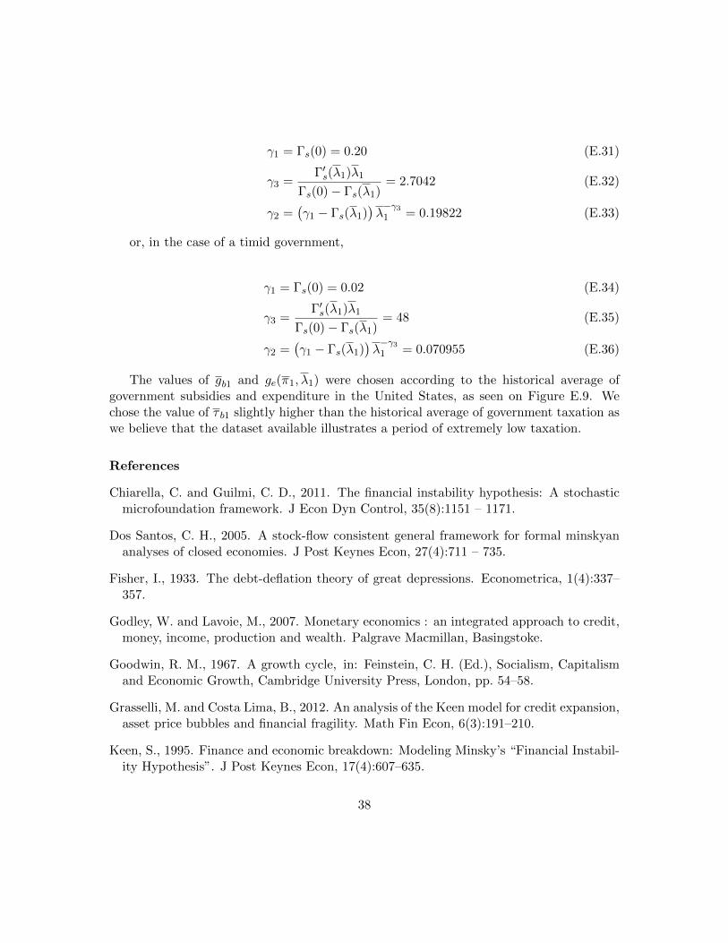
γ1 = Γs(0) = 0.20 (E.31)

γ3 =Γ′s(λ1)λ1

Γs(0)− Γs(λ1)= 2.7042 (E.32)

γ2 =(γ1 − Γs(λ1)

)λ−γ31 = 0.19822 (E.33)

or, in the case of a timid government,

γ1 = Γs(0) = 0.02 (E.34)

γ3 =Γ′s(λ1)λ1

Γs(0)− Γs(λ1)= 48 (E.35)

γ2 =(γ1 − Γs(λ1)

)λ−γ31 = 0.070955 (E.36)

The values of gb1 and ge(π1, λ1) were chosen according to the historical average ofgovernment subsidies and expenditure in the United States, as seen on Figure E.9. Wechose the value of τ b1 slightly higher than the historical average of government taxation aswe believe that the dataset available illustrates a period of extremely low taxation.

References

Chiarella, C. and Guilmi, C. D., 2011. The financial instability hypothesis: A stochasticmicrofoundation framework. J Econ Dyn Control, 35(8):1151 – 1171.

Dos Santos, C. H., 2005. A stock-flow consistent general framework for formal minskyananalyses of closed economies. J Post Keynes Econ, 27(4):711 – 735.

Fisher, I., 1933. The debt-deflation theory of great depressions. Econometrica, 1(4):337–357.

Godley, W. and Lavoie, M., 2007. Monetary economics : an integrated approach to credit,money, income, production and wealth. Palgrave Macmillan, Basingstoke.

Goodwin, R. M., 1967. A growth cycle, in: Feinstein, C. H. (Ed.), Socialism, Capitalismand Economic Growth, Cambridge University Press, London, pp. 54–58.

Grasselli, M. and Costa Lima, B., 2012. An analysis of the Keen model for credit expansion,asset price bubbles and financial fragility. Math Fin Econ, 6(3):191–210.

Keen, S., 1995. Finance and economic breakdown: Modeling Minsky’s “Financial Instabil-ity Hypothesis”. J Post Keynes Econ, 17(4):607–635.

38

Keen, S., 1998. The nonlinear dynamics of debt deflation. Complex Int, 6:1–27.

Minsky, H. P., 1982. Can ‘it’ happen again ? M E Sharpe, Armonk, NY.

Ryoo, S., 2010. Long waves and short cycles in a model of endogenous financial fragility.J Econ Behav Organ, 74(3):163 – 186.

Skott, P., 1989. Effective demand, class struggle and cyclical growth. Int Econ Rev,30(1):231–247.

Smith, H. L. and Thieme, H. R., 2011. Dynamical Systems and Population Persistence.Amer. Math. Soc., Providence, RI.

Taylor, L. and O’Connell, S. A., 1985. A Minsky crisis. Q J Econ, 100:pp. 871–885.

Wray, L. R., 2011. Minsky crisis, in: Durlauf, S. N. and Blume, L. E. (Eds.), The NewPalgrave Dictionary of Economics. Palgrave Macmillan, Basingstoke.

39

0

0.2

0.4

0.6

0.8

1

λ

0

0.1

0.2

0.3

0.4

0.5

d K

0 20 40 60 80 100 120 140 160 180 2000

0.2

0.4

0.6

0.8

1

timeω

ω(0) = 90%, λ(0) = 90%, dk(0) = 10%, g

b(0) = 5%, g

s(0) = 5%, τ

b(0) = 5%, τ

s(0) = 5%, d

g(0) = 0%, r = 3%, r

g = 0.5%, Γ

s(0) = 2%

Keen Model+ Government

0.08

0.09

0.1

0.11

0.12

τ B+

τ S

0

0.1

0.2

0.3

0.4

g E

0

1

2

3

4

d g

0 20 40 60 80 100 120 140 160 180 2000

0.05

0.1

0.15

0.2

time

g B+

g S

Figure 1: Solution to the Keen model with and without a timid government for good initialconditions.

0

0.2

0.4

0.6

0.8

1

λ

0.5

1

1.5

2

2.5

d K

0 20 40 60 80 100 120 140 160 180 2000

0.5

1

1.5

2

time

ω

ω(0) = 75%, λ(0) = 80%, dk(0) = 50%, g

b(0) = 5%, g

s(0) = 5%, τ

b(0) = 5%, τ

s(0) = 5%, d

g(0) = 0%, r = 3%, r

g = 0.5%, Γ

s(0) = 2%

Keen Model+ Government

0.02

0.04

0.06

0.08

0.1

τ B+

τ S

0

0.2

0.4

0.6

0.8

g E

0

2

4

6

8

d g

0 20 40 60 80 100 120 140 160 180 2000

0.02

0.04

0.06

0.08

0.1

time

g B+

g S

Figure 2: Solution to the Keen model with and without a timid government with badinitial conditions.

40

0

0.2

0.4

0.6

0.8

1

λ

0

200

400

600

800

d K

0 20 40 60 80 100 120 140 160 180 2000

1

2

3

4

5

timeω

ω(0) = 75%, λ(0) = 75%, dk(0) = 500%, g

b(0) = 5%, g

s(0) = 5%, τ

b(0) = 5%, τ

s(0) = 5%, d

g(0) = 0%, r = 3%, r

g = 0.5%, Γ

s(0) = 2%

Keen Model+ Government

−10

−5

0

5

τ B+

τ S

0

0.2

0.4

0.6

0.8

1

g E

0

200

400

600

800

d g

0 20 40 60 80 100 120 140 160 180 2000

0.1

0.2

0.3

0.4

time

g B+

g S

Figure 3: Solution to the Keen model with and without a timid government with extremelybad initial conditions.

0

0.2

0.4

0.6

0.8

1

λ

0

1

2

3

4

5

6

d K

0 20 40 60 80 100 120 140 160 180 2000

0.5

1

1.5

2

time

ω

ω(0) = 75%, λ(0) = 75%, dk(0) = 500%, g

b(0) = 5%, g

s(0) = 5%, τ

b(0) = 5%, τ

s(0) = 5%, d

g(0) = 0%, r = 3%, r

g = 0.5%, Γ

s(0) = 20%

Keen Model+ Government

0

0.05

0.1

0.15

0.2

τ B+

τ S

0

0.2

0.4

0.6

0.8

g E

0

2

4

6

8

10

d g

0 20 40 60 80 100 120 140 160 180 2000

0.05

0.1

0.15

0.2

time

g B+

g S

Figure 4: Solution to the Keen model with and without a responsive government withextremely bad initial conditions.

41

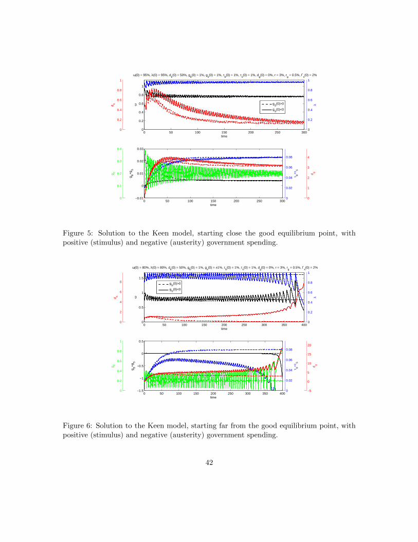
0

0.2

0.4

0.6

0.8

1

λ

0

0.2

0.4

0.6

0.8

1

d K

0 50 100 150 200 250 3000

0.2

0.4

0.6

0.8

1

timeω

ω(0) = 95%, λ(0) = 95%, dk(0) = 50%, g

b(0) = 1%, g

s(0) = 1%, τ

b(0) = 1%, τ

s(0) = 1%, d

g(0) = 0%, r = 3%, r

g = 0.5%, Γ

s(0) = 2%

gS(0)>0

gS(0)<0

0

0.02

0.04

0.06

0.08

τ B+

τ S

0

0.1

0.2

0.3

0.4

g E

0

1

2

3

4

d g

0 50 100 150 200 250 300−0.01

0

0.01

0.02

0.03

time

g B+

g S

Figure 5: Solution to the Keen model, starting close the good equilibrium point, withpositive (stimulus) and negative (austerity) government spending.

0

0.2

0.4

0.6

0.8

1

λ

0

2

4

6

8

d K

0 50 100 150 200 250 300 350 4000

0.5

1

1.5

time

ω

ω(0) = 80%, λ(0) = 80%, dk(0) = 50%, g

b(0) = 1%, g

s(0) = ±1%, τ

b(0) = 1%, τ

s(0) = 1%, d

g(0) = 0%, r = 3%, r

g = 0.5%, Γ

s(0) = 2%

gS(0)>0

gS(0)<0

0

0.02

0.04

0.06

0.08

τ B+

τ S

0

0.2

0.4

0.6

0.8

1

g E

−5

0

5

10

15

20

d g

0 50 100 150 200 250 300 350 400−1.5

−1

−0.5

0

0.5

time

g B+

g S

Figure 6: Solution to the Keen model, starting far from the good equilibrium point, withpositive (stimulus) and negative (austerity) government spending.

42

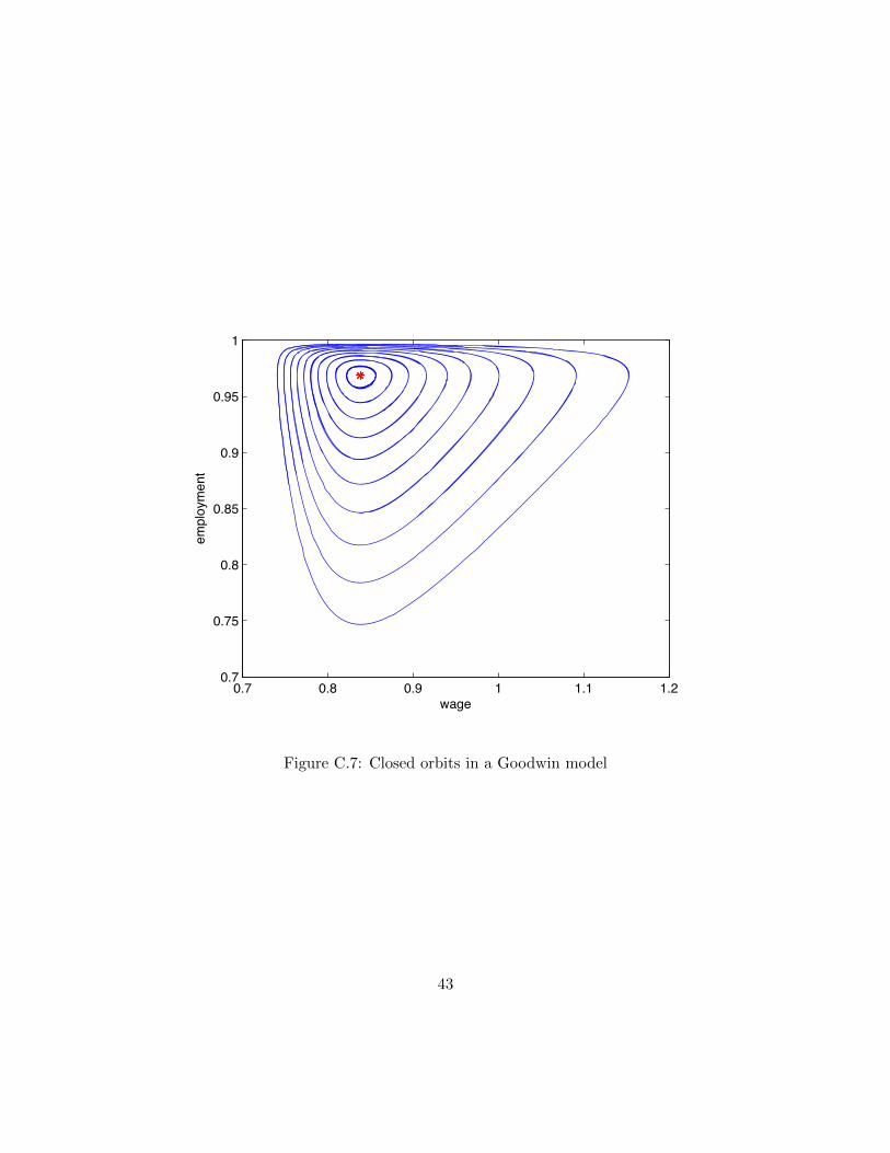
0.7 0.8 0.9 1 1.1 1.20.7

0.75

0.8

0.85

0.9

0.95

1

wage

employment

Figure C.7: Closed orbits in a Goodwin model

43

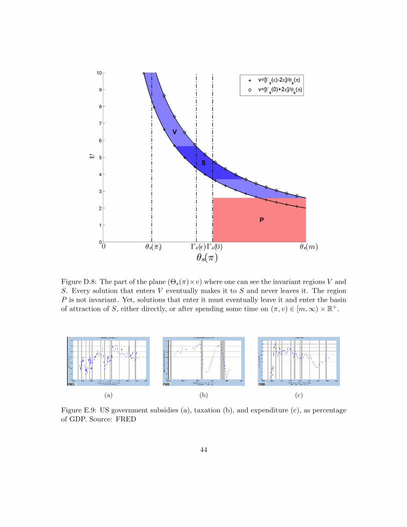
Figure D.8: The part of the plane (Θs(π)×v) where one can see the invariant regions V andS. Every solution that enters V eventually makes it to S and never leaves it. The regionP is not invariant. Yet, solutions that enter it must eventually leave it and enter the basinof attraction of S, either directly, or after spending some time on (π, v) ∈ [m,∞)× R+.

(a) (b) (c)

Figure E.9: US government subsidies (a), taxation (b), and expenditure (c), as percentageof GDP. Source: FRED

44