Despina Petreska* Nikica Mojsoska-Blazevski** ECONOMIC ANNALS, Volume LVIII, No. 197 / April –...
23
23 ECONOMIC ANNALS, Volume LVIII, No. 197 / April – June 2013 UDC: 3.33 ISSN: 0013-3264 * Association for Economic Research, Economic Policymaking and Advocacy “Finance ink”, Skopje, E-mail: despina.petreska@financethink.mk ** University American College-Skopje, E-mail: [email protected] JEL CLASSIFICATION: E21, F21, O16 ABSTRACT: e objective of this paper is to investigate the existence of the Feldstein and Horioka puzzle in transition countries, divided into three groups of countries: South-East Europe (SEE), Central and Eastern Europe (CEE), and the Commonwealth of Independent States (CIS). Central to this puzzle is the β coefficient, which measures the relationship between domestic savings and investment. In their seminal paper from 1980 Feldstein and Horioka estimated a value of the β coefficient close to 1, which in their opinion indicates low capital mobility as opposed to the theory and the conventional wisdom of perfect capital mobility. We use annual data for the period 1991- 2010 and panel cointegration econometric technique to examine this relationship in three panels of countries (SEE, CEE, and CIS). We find that the puzzle of Feldstein and Horioka exists in all three panels, but the connection between savings and investment is generally lower than 1. As we move towards a panel composed of the larger and richer countries the value of the β coefficient increases. Moreover, the coefficient of adjustment of the disequilibrium between domestic savings and investment is positive in all cases, indicating that any imbalance between savings and investment is not corrected immediately. KEY WORDS: Feldstein-Horioka puzzle, domestic savings, investment, capital mobility, panel cointegration, transition economies DOI:10.2298/EKA1397023P Despina Petreska* Nikica Mojsoska-Blazevski** THE FELDSTEIN-HORIOKA PUZZLE AND TRANSITION ECONOMIES
Transcript of Despina Petreska* Nikica Mojsoska-Blazevski** ECONOMIC ANNALS, Volume LVIII, No. 197 / April –...
23
ECONOMIC ANNALS, Volume LVIII, No. 197 / April – June 2013UDC: 3.33 ISSN: 0013-3264
* Association for Economic Research, Economic Policymaking and Advocacy “Finance Think”, Skopje, E-mail: [email protected]
** University American College-Skopje, E-mail: [email protected]
JEL CLASSIFICATION: E21, F21, O16
ABSTRACT: The objective of this paper is to investigate the existence of the Feldstein and Horioka puzzle in transition countries, divided into three groups of countries: South-East Europe (SEE), Central and Eastern Europe (CEE), and the Commonwealth of Independent States (CIS). Central to this puzzle is the β coefficient, which measures the relationship between domestic savings and investment. In their seminal paper from 1980 Feldstein and Horioka estimated a value of the β coefficient close to 1, which in their opinion indicates low capital mobility as opposed to the theory and the conventional wisdom of perfect capital mobility. We use annual data for the period 1991-2010 and panel cointegration econometric technique to examine this relationship in
three panels of countries (SEE, CEE, and CIS). We find that the puzzle of Feldstein and Horioka exists in all three panels, but the connection between savings and investment is generally lower than 1. As we move towards a panel composed of the larger and richer countries the value of the β coefficient increases. Moreover, the coefficient of adjustment of the disequilibrium between domestic savings and investment is positive in all cases, indicating that any imbalance between savings and investment is not corrected immediately.
KEY WORDS: Feldstein-Horioka puzzle, domestic savings, investment, capital mobility, panel cointegration, transition economies
DOI:10.2298/EKA1397023P
Despina Petreska*Nikica Mojsoska-Blazevski**
THE FELDSTEIN-HORIOKA PUZZLE AND TRANSITION ECONOMIES

24
Economic Annals, Volume LVIII, No. 197 / April – June 2013
1. INTRODUCTION
Economists use the term ‘puzzle’ when some empirical facts or findings are inconsistent with the already established theoretical framework(s). One of the most famous puzzles in economics is that of Martin Feldstein and Charles Horioka who, in their seminal paper from 1980 published in the Economic Journal, showed that there is high correlation between domestic savings and investment in conditions of perfect capital mobility. This result is inconsistent with the theory of perfect capital mobility, according to which there should be no link between domestic savings and investment: domestic savings seek the best opportunities for investment and domestic investment will be financed by international financial funds. Therefore Obstfeld and Rogoff (2000) include Feldstein and Horioka’s puzzle in the six major puzzles in international economics.
In the last three decades numerous studies have attempted to explain and solve the Feldstein Horioka puzzle. Some of these empirical studies found high values for the β coefficient and accepted the existence of the puzzle (Penati and Dooley, 1984; Feldstein and Bachetta, 1991; Coakley et al. 2001), whereas another strand of studies (Sinn, 1992; Coakley et al., 2004; Ketenci, 2010) obtained values close to zero and hence declined the claim of Feldstein and Horioka. Between these two (extreme) groups of findings are those who accepted the existence of a high correlation between domestic savings and investment, but not the fact that the high β coefficient indicates low capital mobility. According to them, in countries where perfect capital mobility exists, savings and investment are highly correlated under the influence of some factors such as size of the country (Harberger, 1980; Murphy, 1984), the effect of the European Union (Feldstein and Bachetta, 1991), the degree of development of the country (Dooley et al., 1987; Sinn, 1992; Sinha and Sinha, 2004), the degree of openness of the economy (Bahmani-Oskooee and Chakrabarti, 2005), etc.
The objective of this paper is to investigate the relationship between domestic savings and investment in the transition economies of Central and Southeast Europe (CEE and SEE, respectively) and the Commonwealth of Independent States (CIS), and to put them into a comparative context.
The paper is organized as follows. Section 2 examines in detail the theoretical foundations of the Feldstein-Horioka puzzle, and section 3 establishes an overview and critical review of empirical literature on this topic. Section 4 provides a comparative descriptive analysis of domestic savings and investment in countries of SEE, CEE, CIS, and the Eurozone. Section 5 develops and runs the empirical model. The last section concludes the paper.

FELDStEIN-HORIOKA PUzzLE AND tRANSItION ECONOMIES
25
2. THEORETICAL FOUNDATIONS OF THE FELDSTEIN-HORIOKA PUZZLE
The origin of the Feldstein-Horioka puzzle, which is considered one of the major puzzles in international economics, rests with the seminal paper of Martin Feldstein and Charles Horioka, published in 1980 in Economic Journal, whereby they estimated a cross-section regression of this form:
(I / Y) i = α + β (S / Y) i, i = 1,2,3,4.... N (1)
where I is domestic investment (private and public) in country i, S is domestic savings (private and public) for country i, and Y is GDP. In this equation the coefficient β has the most important role and is called the Feldstein-Horioka coefficient, or the link between domestic savings and investment. The value of β ranges between 0 and 1. If β = 1 there is a 100% correlation between domestic investment and domestic savings. This is an absolute financial autarky, which means that there is no foreign investment in the country, i.e., capital mobility is zero. Another extreme situation is when β = 0, where overall domestic investment is financed with foreign capital, which indicates perfect capital mobility.
In the case of perfect capital mobility, increasing the rate of savings in country i will cause an increase in investment in all countries, where the distribution of increased capital among countries will vary positively with the initial mass of each country’s capital. In the extreme case where country i is very small compared to the global economy, the value of β will be zero. But even for relatively large countries the value of β will be solely determined by the size of their share in the world economy, although on average it will be lower than 0.10. Conversely, estimates of β close to 1 indicate that most of the increased savings in one country remain there.
The Feldstein and Horioka hypothesis is that a high positive correlation between domestic savings and investment indicates low capital mobility. This means that domestic savings are transformed into domestic investment with foreign capital playing a marginal role. to investigate this relationship they used data on national savings, investment, and GDP for 16 OECD countries (Organization for Economic Cooperation and Development)1 for the period 1960-1974. They found a value of the β coefficient close to 1, which contradicts the theory of perfect capital mobility according to which capital moves seeking the highest rates of return. For
1 Australia, Austria, Belgium, Canada, Denmark, Finland, Germany, Greece, Ireland, Italy, Japan, the Netherlands, New zealand, Sweden, the UK, and the USA.

26
Economic Annals, Volume LVIII, No. 197 / April – June 2013
the entire analysed period the β coefficient has a value of 0.89 when using gross savings and investment and 0.94 when using net savings and investment. This means that for every additional US$1 of savings domestic investment increased by US$0.89 or 0.94, respectively. Recognizing that the high coefficient in the relationship between domestic savings and investment may reflect the influence of a third variable, Feldstein and Horioka modify the equation (1) by adding new variables: the rate of population growth, the size of the country, and the openness of the economy. However, they found that these variables are insignificant.
3. REvIEW OF THE EMPIRICAL LITERATURE
The empirical findings of Feldstein and Horioka, along with the current massive capital flows across countries, have initiated plenty of research in this area. Like Feldstein and Horioka (1980) many other economists (Murphy, 1984; Penati and Dooley, 1984; Golub, 1990; Feldstein and Bachetta, 1991; Obstfeld, 1995) performed a cross-section estimation of the relationship between domestic savings and investment for different samples of OECD countries for different time periods. Feldstein and Bachetta (1991), in a sample of 23 OECD countries, showed that, even for the longer period 1960-1986, there is a high correlation between domestic savings and investment, although the β coefficient declined significantly from decade to decade, from 0.91 to 0.61. These authors have identified several reasons for the decline of the β coefficient: reduction of the barriers to international capital flows, development of new markets for hedging and modernization of financial institutions - both leading to facilitation of capital movement - etc. Golub (1990) calculated the β coefficient in a sample of 16 OECD countries for two sub-periods, 1970-1979 and 1980-1986, obtaining the same conclusion as Feldstein and Horioka. Obstfeld and Rogoff (2000) estimated a β coefficient of 0.6 for 24 OECD countries for the period 1990-1997, which is significantly lower than that of Feldstein and Horioka but still much higher than the value expected in a world with fully integrated capital markets.
According to some economists, the use of the cross-section approach in estimating the relationship between savings and investment aims at avoiding some problems in the estimation associated with the possible co-movement of savings and investment over the business cycle (Sinn, 1992). Therefore some economists apply time-series technique to estimate the β coefficient. Sinn (1992) made an empirical test for 23 OECD countries for the period 1960-1988, finding β coefficient values that vary from year to year between 0.4 and 0.9. These values are still high enough to re-confirm the existence of the puzzle. Ghosh and Dutt (2011) used a time series

FELDStEIN-HORIOKA PUzzLE AND tRANSItION ECONOMIES
27
approach on a sample of five countries (USA, UK, France, Japan, and Germany) for the period 1960-2008. Except in France, where β is estimated at a high level of 0.82, for the other four countries low β coefficients were estimated, which refutes the hypothesis of low international capital flows. According to the authors, in these four countries domestic investment is financed by foreign savings (as is the case in the U.S.), or excess domestic savings are invested abroad (as in the case of Japan).
Cooray and Sinha (2005) examined the relationship between domestic savings and investment in 20 poor countries in Africa. Their result showed that the relationship between domestic savings and investment is very low, which means that most investment is financed by foreign rather than domestic savings. However, opposite results are obtained from the estimation of the relationship between domestic savings and investment in three small island states, Mauritius, Malta, and the Maldives (Jain and Sami, 2011). The estimated value of the β coefficient in these countries is very close to 1, indicating that changes in investment are due to changes in domestic savings.
Coakley et al. (2001), through a panel regression for 12 OECD countries for the period 1980-2000, obtained a relatively high value for β of 0.68. However, in their next survey (Coakley et al., 2004) they came to the opposite result, which refutes the high correlation between domestic savings and investment. By adding some variables to the same panel regressions, such as productivity, demographic shocks, heterogeneity of countries and other parameters specific to each country, they obtained a β coefficient lower than 0.3 for all countries, implying that in these countries there is high capital mobility, contrary to their earlier claim.
Many authors accepted the high correlation between savings and investment as empirical evidence, but refused to accept that it indicates low capital mobility (Murphy, 1984; Sinn, 1992; taslim, 1995). They showed that, even in models where perfect capital mobility exists, savings and investment are correlated due to changes in exogenous variables that impact on savings and on investment. According to taslim (1995) these variables are divided into two groups: a) economic growth and population growth that affect the examined variables in the same direction, and b) systematic intervention by government policies that lead to movement in savings and investment. Another reason why savings and investment are highly correlated in the presence of high capital mobility is the ‘country size’ effect, where large countries are expected to rely less on foreign funds for investment (Murphy, 1984; Sinn, 1992). Arguments about the impact of the size of the country are found in two versions (Sinn, 1992). The first one links
28
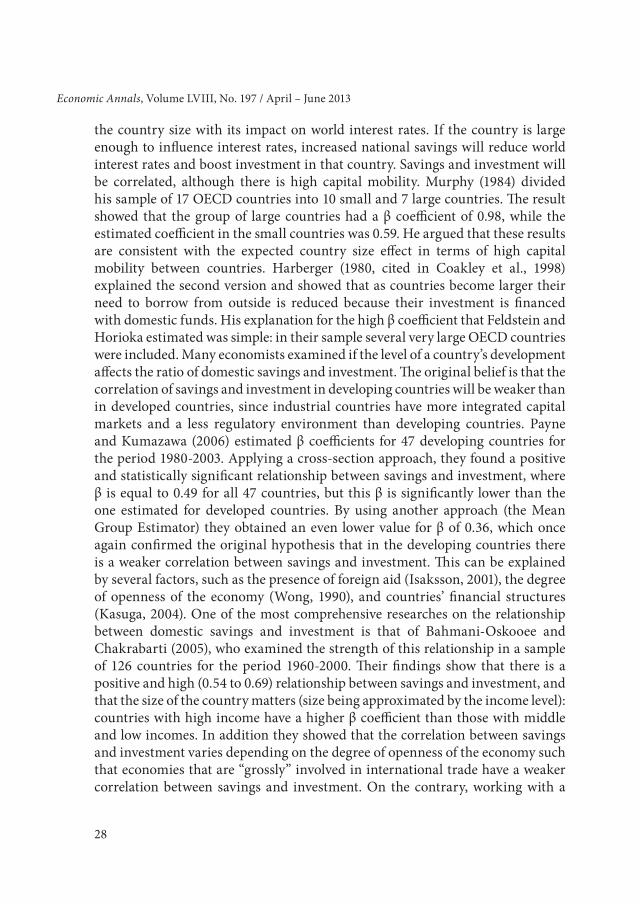
Economic Annals, Volume LVIII, No. 197 / April – June 2013
the country size with its impact on world interest rates. If the country is large enough to influence interest rates, increased national savings will reduce world interest rates and boost investment in that country. Savings and investment will be correlated, although there is high capital mobility. Murphy (1984) divided his sample of 17 OECD countries into 10 small and 7 large countries. The result showed that the group of large countries had a β coefficient of 0.98, while the estimated coefficient in the small countries was 0.59. He argued that these results are consistent with the expected country size effect in terms of high capital mobility between countries. Harberger (1980, cited in Coakley et al., 1998) explained the second version and showed that as countries become larger their need to borrow from outside is reduced because their investment is financed with domestic funds. His explanation for the high β coefficient that Feldstein and Horioka estimated was simple: in their sample several very large OECD countries were included. Many economists examined if the level of a country’s development affects the ratio of domestic savings and investment. The original belief is that the correlation of savings and investment in developing countries will be weaker than in developed countries, since industrial countries have more integrated capital markets and a less regulatory environment than developing countries. Payne and Kumazawa (2006) estimated β coefficients for 47 developing countries for the period 1980-2003. Applying a cross-section approach, they found a positive and statistically significant relationship between savings and investment, where β is equal to 0.49 for all 47 countries, but this β is significantly lower than the one estimated for developed countries. By using another approach (the Mean Group Estimator) they obtained an even lower value for β of 0.36, which once again confirmed the original hypothesis that in the developing countries there is a weaker correlation between savings and investment. This can be explained by several factors, such as the presence of foreign aid (Isaksson, 2001), the degree of openness of the economy (Wong, 1990), and countries’ financial structures (Kasuga, 2004). One of the most comprehensive researches on the relationship between domestic savings and investment is that of Bahmani-Oskooee and Chakrabarti (2005), who examined the strength of this relationship in a sample of 126 countries for the period 1960-2000. Their findings show that there is a positive and high (0.54 to 0.69) relationship between savings and investment, and that the size of the country matters (size being approximated by the income level): countries with high income have a higher β coefficient than those with middle and low incomes. In addition they showed that the correlation between savings and investment varies depending on the degree of openness of the economy such that economies that are “grossly” involved in international trade have a weaker correlation between savings and investment. On the contrary, working with a
FELDStEIN-HORIOKA PUzzLE AND tRANSItION ECONOMIES
29
sample of 123 countries, Sinha and Sinha (2004) found that capital mobility was higher in lower income countries.
4. DESCRIPTIvE ANALYSIS
This section provides a descriptive and comparative analysis of the data used in the econometric model in part 5, in order to build intuition about econometric modelling. For this purpose, first we provide a comparative analysis of gross savings and investment in the SEE, CEE, and CIS countries and the Eurozone, and later in the analysis we include other factors that may affect the relationship between domestic savings and investment.
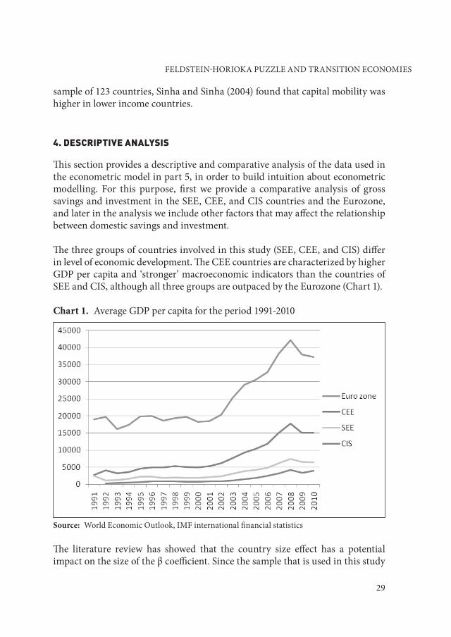
The three groups of countries involved in this study (SEE, CEE, and CIS) differ in level of economic development. The CEE countries are characterized by higher GDP per capita and ‘stronger’ macroeconomic indicators than the countries of SEE and CIS, although all three groups are outpaced by the Eurozone (Chart 1).
Chart 1. Average GDP per capita for the period 1991-2010
Source: World Economic Outlook, IMF international financial statistics
The literature review has showed that the country size effect has a potential impact on the size of the β coefficient. Since the sample that is used in this study

30
Economic Annals, Volume LVIII, No. 197 / April – June 2013
is mainly composed of small countries, with the relative exceptions of Romania (SEE group) and Russia (CIS group), under the influence of this effect we expect to obtain a lower value of the savings-investment coefficient in CIS than in SEE and CEE, and a lower value in SEE than in CEE, as compared with the β coefficient for OECD countries that Feldstein and Horioka estimated in 1980. As a measure of the size of the countries included in this study we use the population size, presented in Chart 2.
Chart 2. Average population in 2010, in millions
Source: World Economic Outlook, IMF international financial statistic Note: * Russia is excluded from the CIS sample because, with a population of 143 million, it significantly affects the average population in this group and gives a distorted picture
table 1 in the Appendix presents data on gross savings and investment in the three groups of countries and the Eurozone average. Data show that as we move towards more developed and larger countries the gross domestic savings have a larger share of gross domestic product. This ratio is 0.201 for CEE countries and 0.213 for the member states of the Eurozone. Also, as we move towards the more developed group of countries the standard deviation increases, which is an indication that the group of developed countries is composed of more heterogeneous countries in terms of savings. These findings do not apply to CIS countries, where the standard deviation of the gross savings equals 0.130, implying a variability that is several times higher than in the other countries.

FELDStEIN-HORIOKA PUzzLE AND tRANSItION ECONOMIES
31
For example, in Georgia the average ratio of gross savings to GDP is -0.16, which means there are negative savings in this country, while Russia’s gross savings equal 0.29 of gross domestic product (see the first column of table 1).
The corresponding ratios between gross investment and gross domestic product in the SEE countries are more concentrated around the average value. Among the seven SEE countries the 20-year average ratio of gross investment to GDP is 0.229 and the standard deviation 0.023.
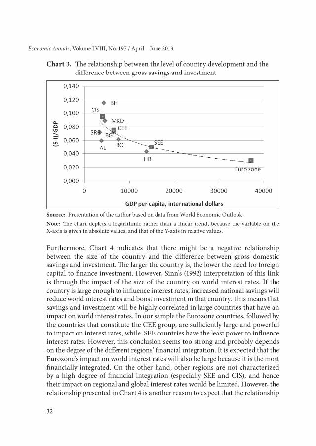
Differences in the rates of gross domestic savings and investment relative to GDP are given in the last column of table 1. According to the basic macroeconomic equations the difference between savings and investment is equal to the current account, which shows how much investment is financed with foreign capital (savings). The difference in our case declines as it moves towards the more developed groups of countries. This potentially negative relationship between the degree of development of the country (measured by the GDP per capita) and the difference in the rates of gross savings and investment can be seen in Chart 3. At first glance it is evident that as the country becomes richer (has a higher GDP per capita) the difference between gross domestic savings and investment is smaller. This is another indication of Harberger’s claim (1980) that as countries become richer their need to borrow externally is reduced because their investment can be financed with domestic funds. However, note that the chart is indicative of the relationship, but cannot imply a causal relationship. We will test the potential causality with the econometric model. Here our task is to build intuition about the estimation results: we expect that the β coefficient will decrease with the reduction of the level of country development. That means that the β coefficient would have the lowest value for CIS and a higher value for SEE, while for CEE it would be higher than for both CIS and SEE.
32
Economic Annals, Volume LVIII, No. 197 / April – June 2013
Chart 3. the relationship between the level of country development and the difference between gross savings and investment
Source: Presentation of the author based on data from World Economic OutlookNote: The chart depicts a logarithmic rather than a linear trend, because the variable on the X-axis is given in absolute values, and that of the Y-axis in relative values.
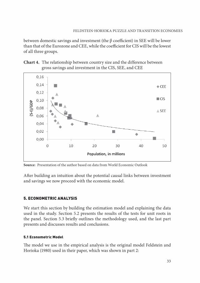
Furthermore, Chart 4 indicates that there might be a negative relationship between the size of the country and the difference between gross domestic savings and investment. The larger the country is, the lower the need for foreign capital to finance investment. However, Sinn’s (1992) interpretation of this link is through the impact of the size of the country on world interest rates. If the country is large enough to influence interest rates, increased national savings will reduce world interest rates and boost investment in that country. This means that savings and investment will be highly correlated in large countries that have an impact on world interest rates. In our sample the Eurozone countries, followed by the countries that constitute the CEE group, are sufficiently large and powerful to impact on interest rates, while. SEE countries have the least power to influence interest rates. However, this conclusion seems too strong and probably depends on the degree of the different regions’ financial integration. It is expected that the Eurozone’s impact on world interest rates will also be large because it is the most financially integrated. On the other hand, other regions are not characterized by a high degree of financial integration (especially SEE and CIS), and hence their impact on regional and global interest rates would be limited. However, the relationship presented in Chart 4 is another reason to expect that the relationship
FELDStEIN-HORIOKA PUzzLE AND tRANSItION ECONOMIES
33
between domestic savings and investment (the β coefficient) in SEE will be lower than that of the Eurozone and CEE, while the coefficient for CIS will be the lowest of all three groups.
Chart 4. the relationship between country size and the difference between gross savings and investment in the CIS, SEE, and CEE
Source: Presentation of the author based on data from World Economic Outlook
After building an intuition about the potential causal links between investment and savings we now proceed with the economic model.
5. ECONOMETRIC ANALYSIS
We start this section by building the estimation model and explaining the data used in the study. Section 5.2 presents the results of the tests for unit roots in the panel. Section 5.3 briefly outlines the methodology used, and the last part presents and discusses results and conclusions.
5.1 Econometric Model
The model we use in the empirical analysis is the original model Feldstein and Horioka (1980) used in their paper, which was shown in part 2:
34
Economic Annals, Volume LVIII, No. 197 / April – June 2013
(I / Y) i, t = α + β (S / Y) i, t + ui, t i = 1,2,3,4.... N; t = 1,2,3,4.... N (2)
where I is domestic investment (private and public) for country i at time t, S is domestic savings (private and public), Y is GDP, and ui,t is the error term satisfying N ~ (0,1). β is the ratio which is of central importance in this study, and which shows the relationship between domestic savings and investment and is an indicator of capital mobility in the analyzed countries.
Given that we would like to examine how the three variables mentioned in part 3 (openness of the economy, population growth, and size of the country) potentially affect the saving-investment relationship (i.e., whether and how their inclusion in the analysis changes the β coefficient) we will upgrade model (2) by adding these variables. The extended model has the following form:
(I / Y) i, t = α + β (S / Y) i, t + γ1X1, i, t + γ2H2, i, t + γ3H3, i, t + ui, t (3)
where X1,i,t is a measure of openness of the country represented as a share of trade (exports and imports) in GDP, X2,i,t is a measure of annual population growth, and X3,i,t is a measure of country size presented as a logarithm of GDP. The decision to include these variables in the model is based on the similar approach used by Sinn (1992) and Harberger (1980), elaborated in Section 3. Based on these factors, in the previous section we expected that in our panel of countries we would obtain lower values for the β coefficient compared to those that Feldstein and Horioka estimated in their seminal paper, and that as we move towards the panels composed of smaller and less developed countries the value of the β coefficient will decrease.
In their paper Feldstein and Horioka (1980) used a cross-section approach to estimate the relationship between domestic savings and investment, but in this study we will use panel co-integration for estimating this relationship in the panels of countries, an econometric technique that is elaborated in the following sections.
to test the econometric model we use data from three groups of countries, SEE, CIS, and CEE, from after they abandoned a planned economy in 1991/92 until 2010. Montenegro and Kosovo are excluded from the SEE panel due to lack of data. turkmenistan is excluded from the CIS panel for the same reason. 1992 is the initial year of the analysis.
FELDStEIN-HORIOKA PUzzLE AND tRANSItION ECONOMIES
35
The models for all three panels used annual data for gross domestic savings, investment, trade, gross domestic product, and population. The first three variables (domestic savings, investment, and trade) are expressed as a percentage of GDP, and the population variable is included as an annual rate of growth. Data is from the database of the International Monetary Fund (World Economic Outlook), World Development Indicators, and the national statistical offices of the individual countries.
5.2 Unit roots
We first test whether variables contain a unit root within the panels of countries, using the panel unit roots from the first and the second generation (Holmes et al., 2010). The difference between them is that the first ones are based on the assumption of cross independence among the examined units (in our case, countries), while the latter are based on an assumption of cross-dependency among the units in the form of a single unobserved common factor. The assumption of cross-dependence in macroeconomics is particularly important because of the growing trade and financial integration of countries. This is confirmed by the current financial crisis, which spread very rapidly around the world. Therefore ignoring this dependence may lead to erroneous results.
The results of two tests for panel unit roots are presented in table 2 for the order of the time lag of the autoregressive parameters from 0 to 2. The test includes a trend, due to the general observation from part 4 that the series of savings and investment are trending. The null hypothesis in both tests is that the series contain a unit root. Madalla and Wu’s (1999) test of the first generation (no cross-dependence) is shown at the top of the table, and the test of Pesaran (2007) from the second generation (cross-dependence) in the lower part. According to the Madalla and Wu (1999) test, in most cases the null hypothesis of a unit root is rejected even at the 1% level. However, the results of the Pesaran test (2007) suggest that at higher values of the time lag the null hypothesis for the existence of a unit root cannot be rejected in most cases. taking a higher order of the time lag (in this case 2) is logical, due to the likely existence of serial correlation in the series.
table 3 shows the test of Pesaran (2004) for cross-dependence among countries and suggests that the null hypothesis for no cross-dependence is rejected in most cases. The null hypothesis is not rejected only in the case of savings in CEE and SEE, but for these two series the Madalla and Wu (1999) test did not reject the hypothesis of the unit root for higher ranks of the time lag. So, the second test

36
Economic Annals, Volume LVIII, No. 197 / April – June 2013
gives a more relevant picture of the unit roots in our case, and hence the results from the first test should be taken with caution.
According to these findings we have enough evidence to conclude that the series of savings and investment likely follow a non-stationary process; i.e., contain a unit root.
5.3 Methodology
The findings of part 5.2 indicated that the series for the savings and investment in the panels of countries probably contain one unit root. Therefore we continue our analysis in order to establish a long-term relationship between savings and investment as a percentage of GDP. In other words, we examine whether there exists a cointegration relationship between these two variables. Panel cointegration analysis begins with the test for the existence of a panel cointegration relationship, originally developed by Westerlund (2007). The advantage of this test is that it takes into account the possibility of the existence of multiple structural changes in the series.
The general structure of the model for error correction in a panel context, based on the existence of a cointegration relationship, has the following form:
(4)
where λi is the term for error correction / speed of adjustment, yit the matrix of K observable endogenous variables, and xit the matrix of M observable variables. Notice that the penultimate term in (4) includes past and future values; otherwise we should assume full erogeneity of x. aij marks short-term parameters, which as well as σ2
i vary between countries, and uit is the matrix of errors. βi is the coefficient in front of the variables of the long-term vector (the coefficient that is our interest in this paper). There are several estimators of the model (4), of which the Pooled Mean Group Estimator of Pesaran et al. (1999) has the greatest practical application. It has the following form (a slight modification of 4):
(5)
In this estimator the error correction term λi varies between countries, while the parameters Θ and βi are constant between groups. The advantage of this estimator is that it works better in small samples of similar countries than in a large variety of macro panels (Pesaran et al. 1999). It also gives consistent results when the

FELDStEIN-HORIOKA PUzzLE AND tRANSItION ECONOMIES
37
long-term relationship includes a stationary and a non-stationary variable (which is not an issue in our analysis). It adapts to the problem of endogeneity of the variables, which if not taken into account results in biased results. As Pesaran points out, this dynamic approach to panel estimation seems appropriate in cases when there are “... good reasons to expect the long-term equilibrium relationships between variables to be similar between countries, due to the budget constraint or solvency condition ...” (p. 621) that affects all countries in a similar way. The latter is a realistic assumption for countries that are similar to each other and/or formed one country in the past.
5.4 Results and discussion
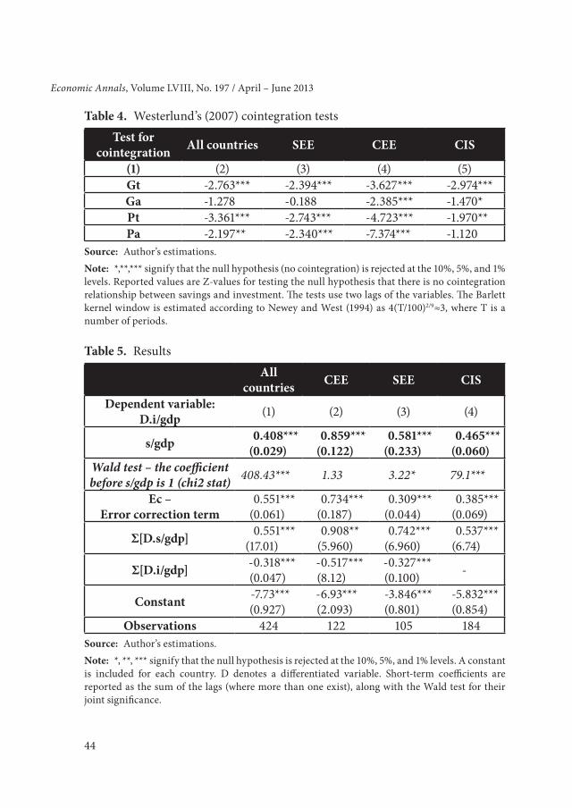
As we mentioned in part 5.3, the starting point in cointegration analysis is the test of Westerlund (2007) for the existence of a panel cointegration relationship. table 4 shows the results of this panel test for the countries involved in this research. The results for the existence of a cointegartion in the panel composed of all countries shows that only the second test does not reject the null hypothesis according to which there is no cointegration between the series on savings and investment. Series of savings and investment in the countries of SEE are cointegrated according to three out of four of Westerlund’s tests (2007). In the CEE countries all four tests reject the null hypothesis that there is no cointegration between series. Across CIS countries three tests reject the null hypothesis, although one of them only at the 10% level of probability, and the fourth test does not reject the null hypothesis. The weaker results for the tests in CIS are to be expected, due to the finding in part 4 that this group of countries has the greatest variability of the series of investment and savings. According to this, the analysis of the panel cointegration relationships in table 4 gives enough empirical evidence that all four panels contain a cointegration relationship between savings and investment.
The results for the value of the β coefficient and other parameters obtained for the panels of countries using the PMG estimator are shown in table 5. The coefficient β that is of central importance in this work is shown in the first row of the table (in bold characters). Column 1 gives the results for the panel composed of all transition countries. The β coefficient is 0.41 and is statistically significant and statistically different from 1 (according to the Wald test in row 2, in italic characters). However this value seems very small, given the heterogeneity of the panel, and cannot be reconciled for all countries, especially for the more developed countries such as in CEE. Thus, the results of the entire panel of transition countries should be taken with caution. We proceed by looking separately at the three groups of countries, CEE, SEE, and CIS, in accordance with the discussion
38
Economic Annals, Volume LVIII, No. 197 / April – June 2013
of the different levels of economic development of these groups mentioned in part 4.
Our suspicion is confirmed if we consider the results separately for each panel, shown in columns 2, 3, and 4 in table 5. In all three groups the β coefficient is statistically significant at the 1% level of probability that indicates a significant long-term relationship between savings and investment in these countries. A second feature of the results is that as we move from CEE to SEE and to CIS (high to low level of economic development) the β coefficient decreases. The highest value of 0.86 is measured in the CEE panel, in SEE it is 0.58, and the lowest value of 0.47 is measured in the CIS panel. This is in line with our intuition, established in part 4, that as countries become bigger and richer their need to borrow externally decreases, because they create enough domestic savings to finance their investment. In terms of Feldstein and Horioka’s belief that the β coefficient is an indicator of the capital mobility between countries, we may conclude that capital mobility is potentially the highest in the least developed countries (in our case CIS), whereas as we move towards a panel of developed countries it decreases. In other words, the puzzle is relevant to the examined countries.
The original idea of Feldstein and Horioka can be examined using the Wald test, where we set the null hypothesis that the β coefficient is equal to 1. Except for CEE, where we cannot reject this hypothesis (which is expected because the ratio is 0.86 and is very close to 1), all other panels cannot accept null hypothesis even at the 10% level of probability. This indicates that CEE countries probably reached a high enough level of economic development with self-generated domestic savings to finance their own investment. This is not the case in SEE and CIS, which still rely on foreign savings, and where the need for foreign savings is probably greater in CIS than in SEE.
The term for error correction is positive and statistically significant in all cases. This term assesses the speed of adjustment of the dependent variable to the equilibrium level, and in most cases has a negative value. The statistical significance of this term suggests that investment is driven by the growth of domestic savings. However, the positive value implies that the disequilibrium in the investment-domestic savings relationship is not adjusted after the shock, but is further deepened (Harris and Sollis, 2003). This probably indicates that a change in domestic savings - for example, by reducing taxes on interest on deposits - causes a delayed reaction in investment. Countries may not be able to adapt immediately, so they begin to borrow intensively externally, rather than reduce the volume of investment.

FELDStEIN-HORIOKA PUzzLE AND tRANSItION ECONOMIES
39
table 5 in the following section gives results for the short-term dynamics, which give the cumulative coefficients with the Wald test for their joint statistical significance, where applicable. Their inclusion is mainly for statistical reasons, in order to take into account the possible existence of a serial correlation in the model.
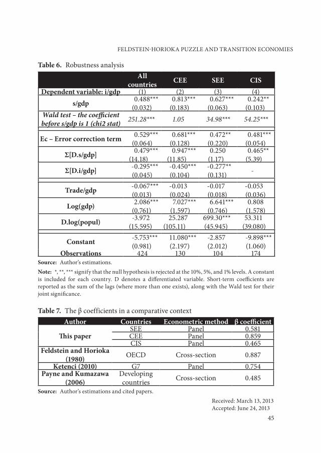
table 6 shows the results of the robustness analysis, with the basic model being upgraded with three additional variables: the openness of the country (represented as total trade to GDP), the annual growth rate of population, and the country size (represented as the logarithm of GDP). In all specifications the β coefficient, the coefficient of adjustment, and the short-run coefficients do not change their magnitude and statistical significance. Hence we conclude that the results of table 5 are quite robust to the addition of the three variables.
Notice that the three variables are added as endogenous in the model (5), as elaborated in Section 5.3. These variables are tested for unit roots, but to save space the results are available upon request. They suggest the existence of a unit root in the form in which they enter into the model. trade openness is statistically significant only in the panel of all transition countries, but if we look at the panels separately it loses statistical significance at any statistical level. This may indicate that the importance of the entire panel is distorted or baseless. Additionally, this variable has an unexpected negative sign. Thus, as in the Feldstein and Horioka study, we have no arguments to support the opinion that greater openness is important for the domestic savings-investment relationship. For the other two variables we can see limited significance, indicating that country size can have some impact on the saving-investment relationship (which is in line with our elaboration of the basic results). However the evaluated coefficients are very small, indicating an increase in investment to GDP ratio by about 0.07 percentage points when GDP grows by 1% in CEE and SEE. The population is significant only in SEE, indicating a growth of investment to GDP ratio by 7 percentage points when the population grows by 1%. This ratio is not surprising if one considers the 2.8% per year average population growth in the observed period.
6. CONCLUSION
In this paper we estimated the domestic savings-investment relationship for panels of transition countries using panel cointegration method. The results for the value of the β coefficient indicated that as we move towards the panel composed of larger and richer countries the value of the β coefficient increases.
40
Economic Annals, Volume LVIII, No. 197 / April – June 2013
If this ratio is taken as an indicator of capital mobility it means that larger and richer countries are characterized by lower capital mobility. This is another proof of the existence of the Feldstein-Horioka puzzle in the countries examined in this research.
table 7 in the Appendix compares the results of this survey with those in some of the literature outlined in part 3. The comparison indicates that the this paper’s resulting coefficient for CEE is in the magnitude of the OECD and Group of Seven industrialized countries, which indicates that in terms of the saving-investment relationship (i.e., the need for foreign savings) CEE countries are closer to the developed countries. The value of the β coefficient in CIS is in line with that for the groups of developing countries. The result for SEE is somewhere in the middle. We should emphasize that this comparison is only indicative because: i) the comparative papers relate to other time periods that were often before the period we examine in this paper, and ii) a fraction of the studies elaborated in part 2 found very low or insignificant values for the β coefficient, which is contrary to the assertion of Feldstein and Horioka and the findings of this paper.
Another important finding of this paper is the statistical significance of the coefficient of adjustment of the disequilibrium between domestic savings and investment. The coefficient in all cases is found to be positive, indicating that any imbalance between savings and investment is not corrected immediately, but at the first step is further deepened. Practically, this means that when savings in these countries decline for any reason, countries do not reduce the level of investment but resort to foreign savings.
REFERENCES
Bahmani-Oskooee, M. & Chakrabarti, A. (2005). Openness, size and the saving-investment relationship. Economic Systems, 29, pp. 283-293.
Coakley, J., Fuertes, A. M. & Spagnolo, F. (2001). The Feldstein-Horioka Puzzle is not as bad as you think (Working paper series WP01-07), Financial econometrics research center.
Coakley, J., Fuertes, A. M. & Spagnolo, F. (2004). Is the Feldstein-Horioka Puzzle history? The Manchester school, 71 (5), pp. 569-590.
FELDStEIN-HORIOKA PUzzLE AND tRANSItION ECONOMIES
41
Coakley, J., Kulasi, F. & Smith, R. (1998). The Feldstein-Horioka Puzzle and capital mobility: A review. International journal of finance and economics, 3, pp. 169-188.
Cooray, A. & Sinha, D. (2005). The Feldstein-Horioka model re-visited for African countries, Applied Economics, 39 (12), pp. 1501-1510.
Dooley, M., Frankel, J. & Mathieson, D. (1987), International capital mobility: what do saving-investment correlations tell us? IMF stuff papers, 34 (3), pp. 503-530.
Feldstein, M. (1983). Domestic saving and international capital movements in the long run and the short run. European economic review, 21, pp. 129-151.
Feldstein, M. & Bachetta, P. (1991). National savings and international investment. In D. Berheim and J. Shoven (Eds.), National saving and economic performance (pp. 201-226). Chicago, University of Chicago Press.
Feldstein, M. & Horioka, C. (1980). Domestic saving and international capital flows. Economic Journal, 90, pp. 314–329.
Ghosh, D. & Dutt, S. (2011). International capital mobility and the Feldstein-Horioka Puzzle: an empirical examination for the G5 nations. Southwestern economic review, 38(1), pp. 27-36.
Golub, S. S. (1990). International capital mobility: net versus gross stocks and flows. Journal of international money and finance, 9, pp. 424-439.
Harberger, A. (1980). Vignettes on the world capital market. American economic review, 70, pp. 331-337.
Harris, R. & Sollis, R. (2003). Applied Time Series Modeling and Forecasting. Chichester: John Wiley & Sons Ltd.
Holmes, ark J., Otero, J. & Panagiotidis, t. (2010). Are EU budget deficits stationary? Empirical economics, 38 (3), pp. 767-778.
Isaksson, A. (2001). Financial liberalization, foreign aid, and capital mobility: Evidence from 90 developing countries. Journal of international financial markets, institutions, and money, 11, pp. 309–338.
Jain, V. & Sami, J. (2011). Capital mobility and saving-investment nexus empirical evidence from Mauritius, Malta and Maldives. ICOQM-10, pp. 207-213.
Kasuga, H. (2004). Saving–Investment Correlations in Developing Countries. Economics Letters, 83, pp. 371–376.
Ketenci, N. (2010). The Feldstein Horioka Puzzle by groups of OECD members: the panel approach. (MPRA paper, 25848).

42
Economic Annals, Volume LVIII, No. 197 / April – June 2013
Maddala, G. S. & Wu, S. (1999). A comparative study of unit root tests with panel data and a new simple test. Oxford bulletin of economics and statistics, 61 (special issue), pp. 631-652.
Murphy, R. G. (1984). Capital mobility and the relationship between saving and investment rates. Journal of international money and finance, 3, pp. 327-342.
Obstfeld, M. (1995). International capital mobility in the 1990s. In P.B. Kenen (Eds.), Understanding interdependence: The macroeconomics of the open economy, Princeton: Princeton University Press.
Obstfeld, M. & Rogoff, K. (2000). The six major puzzles in international macroeconomics: is there a common cause? (NBER working paper series, 7777).
Payne, J. E. & Kumazawa, R. (2006). Capital mobility and the Feldstein-Horioka Puzzle: Re-examination of less developed countries. The Manchester School, 74 (5), pp. 610-616.
Penati, A. & Dooley, M. (1984). Current account imbalances and capital formation in the industrialized countries. IMF stuff papers, 31, pp. 1-24.
Pesaran, M. H. (2004). General diagnostic tests for cross section dependence in panels. (IZA discussion paper, 1240).
Pesaran, M. H. (2007). A simple panel unit root test in the presence of cross-section dependence. Journal of Applied Econometrics, 22(2), pp. 265-312.
Pesaran, M. H., Shin, Y., & Smith, R. (1999), Pooled mean group estimation of dynamic heterogeneous panels. Journal of the American Statistical Association, 94, pp. 289-326.
Sinha, t. & Sinha, D. (2004). The mother of all puzzles would not go away. Economic Letters, 82, pp. 259-267.
Sinn, S. (1992). Saving-investment correlations and capital mobility: on the evidence from annual data. The economic journal, 102, pp. 1162-1170.
taslim, M. A. (1995). Saving investment correlation and capital mobility. (UNE working papers in economics, 18).
Westerlund, J. (2007). testing for Error correction in panel data. Oxford bulletin of economics and statistics, 69 (6), pp. 709-748.
Wong, D. Y. (1990). What do saving-investment relationships tell us about capital mobility? Journal of international money and finance, 9, pp. 60-74.
Wooldridge, J.M. (2007). Introductory Econometrics: A Modern Approach. 3rd edition, London: The MIt Press.

FELDStEIN-HORIOKA PUzzLE AND tRANSItION ECONOMIES
43
APPENDIx
Table 1. Average values of gross domestic savings and investment in the period 1991-2010
Panel S/GDP I/GDP [S-I]/GDP
Average SEE 0.154(0.029)
0.229(0.023)
0.075(0.024)
Average CIS 0.172(0.130)
0.252(0.047)
0.095(0.114)
Average CEE 0.201(0.034)
0.251(0.030)
0.050(0.028)
Average Euro zone 0.213(0.045)
0.224(0.030)
0.040(0.030)
Source: World Economic Outlook; IMF international finance statistics and author’s estimationsNote: Values shown in parentheses are standard deviations.
Table 2. Panel unit rootsi/gdp s/gdp
All SEE CEE CIS All SEE CEE CIStime
lag (1) (2) (3) (4) (5) (6) (7) (8)
Madalla and Wu (1999)
0 174.37*** 17.459 6.875 89.82*** 181.25*** 71.257*** 67.086*** 103.12***1 174.86*** 50.835*** 36.55*** 97.92*** 166.77*** 31.801*** 26.100* 98.42***2 131.86*** 23.538 35.13*** 61.27*** 96.31 16.854 47.054 44.32***
Pesaran (2007)
0 -4.403*** -0.466 -1.616* -2.947*** -2.881*** -2.710*** -3.474*** -3.575***1 -3.967*** -0.784 -1.100 -4.774*** -1.403* 1.107 -0.339 -2.204*2 -0.167 -1.670* 0.711 -2.218* 0.780 -0.164 0.568 0.634
Source: Author’s estimations.Note: *,**,*** signify that the null hypothesis (has unit root) is rejected at the 10%, 5%, and 1% levels of probability. Reported values for the Madalla and Wu (1999) test are chi2 values. Reported values for the Pesaran test (2007) are z t-bar values. The tests include trend, due to the general conclusion from Part 3 that series for investment and savings are trending.
Table 3. test for cross-dependence among countriesAll countries SEE CEE CIS
s/gdp 7.34*** -0.36 -0.19 8.85***i/gdp 4.20*** 4.20*** 9.50*** 5.00***
Source: Author’s estimations.Note: *,**,*** signify that the null hypothesis (no cross dependence among countries) is rejected at the 10%, 5%, and 1% levels of probability. Reported values for the Pesaran test are CD values.
44
Economic Annals, Volume LVIII, No. 197 / April – June 2013
Table 4. Westerlund’s (2007) cointegration tests Test for
cointegration All countries SEE CEE CIS
(1) (2) (3) (4) (5)Gt -2.763*** -2.394*** -3.627*** -2.974***Ga -1.278 -0.188 -2.385*** -1.470*Pt -3.361*** -2.743*** -4.723*** -1.970**Pa -2.197** -2.340*** -7.374*** -1.120
Source: Author’s estimations.Note: *,**,*** signify that the null hypothesis (no cointegration) is rejected at the 10%, 5%, and 1% levels. Reported values are z-values for testing the null hypothesis that there is no cointegration relationship between savings and investment. The tests use two lags of the variables. The Barlett kernel window is estimated according to Newey and West (1994) as 4(Т/100)2/9≈3, where t is a number of periods.
Table 5. ResultsAll
countries CEE SEE CIS
Dependent variable: D.i/gdp (1) (2) (3) (4)
s/gdp 0.408***(0.029)
0.859***(0.122)
0.581***(0.233)
0.465***(0.060)
Wald test – the coefficient before s/gdp is 1 (chi2 stat) 408.43*** 1.33 3.22* 79.1***
Ec – Error correction term
0.551***(0.061)
0.734***(0.187)
0.309***(0.044)
0.385***(0.069)
Σ[D.s/gdp] 0.551***(17.01)
0.908**(5.960)
0.742***(6.960)
0.537***(6.74)
Σ[D.i/gdp] -0.318***(0.047)
-0.517***(8.12)
-0.327***(0.100) -
Constant -7.73***(0.927)
-6.93***(2.093)
-3.846***(0.801)
-5.832***(0.854)
Observations 424 122 105 184Source: Author’s estimations.Note: *, **, *** signify that the null hypothesis is rejected at the 10%, 5%, and 1% levels. A constant is included for each country. D denotes a differentiated variable. Short-term coefficients are reported as the sum of the lags (where more than one exist), along with the Wald test for their joint significance.
FELDStEIN-HORIOKA PUzzLE AND tRANSItION ECONOMIES
45
Table 6. Robustness analysisAll
countries CEE SEE CISDependent variable: i/gdp (1) (2) (3) (4)
s/gdp 0.488***(0.032)
0.813***(0.183)
0.627***(0.063)
0.242**(0.103)
Wald test – the coefficient before s/gdp is 1 (chi2 stat) 251.28*** 1.05 34.98*** 54.25***
Ec – Error correction term 0.529***(0.064)
0.681***(0.128)
0.472**(0.220)
0.481***(0.054)
Σ[D.s/gdp] 0.479***(14.18)
0.947***(11.85)
0.250(1.17)
0.465**(5.39)
Σ[D.i/gdp] -0.295***(0.045)
-0.450***(0.104)
-0.277**(0.131) -
Trade/gdp -0.067***(0.013)
-0.013(0.024)
-0.017(0.018)
-0.053(0.036)
Log(gdp) 2.086***(0.761)
7.027***(1.597)
6.641***(0.746)
0.808(1.578)
D.log(popul) -3.972(15.595)
25.287(105.11)
699.30***(45.945)
53.311(39.080)
Constant -5.753***(0.981)
11.080***(2.197)
-2.857(2.012)
-9.898***(1.060)
Observations 424 130 104 174Source: Author’s estimations.Note: *, **, *** signify that the null hypothesis is rejected at the 10%, 5%, and 1% levels. A constant is included for each country. D denotes a differentiated variable. Short-term coefficients are reported as the sum of the lags (where more than one exists), along with the Wald test for their joint significance.
Table 7. the β coefficients in a comparative contextAuthor Countries Econometric method β coefficient
This paperSEE Panel 0.581CEE Panel 0.859CIS Panel 0.465
Feldstein and Horioka (1980) OECD Cross-section 0.887
Ketenci (2010) G7 Panel 0.754Payne and Kumazawa
(2006)Developing countries Cross-section 0.485
Source: Author’s estimations and cited papers.Received: March 13, 2013Accepted: June 24, 2013