Designs for Muon Tomography Station Prototypes Using GEM ... · iv I designed and ran simulations...

Designs for Muon Tomography Station Prototypes Using

GEM Detectors

by

Leonard Victor Grasso III

Bachelors Degree in Physics

University of Florida, 1998

A thesis

submitted to

Florida Institute of Technology

in partial fulfillment of the requirements

for the degree of

Master of Science

In Physics

Melbourne, Florida

May, 2012

©Copyright 2012 Leonard V. Grasso III

All Rights Reserved

The author grants permission to make copies.

_________________________

We the undersigned committee hereby recommend

that the attached document be accepted as fulfilling in

part the requirements for the degree of

Master of Science in Physics.

“Designs for Muon Tomography Station Prototypes Using GEM Detectors,” a

thesis by Leonard Victor Grasso III

_____________________________

Marcus Hohlmann, Ph.D.

Associate Professor

Physics and Space Sciences

_____________________________

Debasis Mitra, Ph.D.

Professor

Computer Sciences

_____________________________

Ming Zhang, Ph.D.

Professor


_____________________________

Terry D. Oswalt, Ph.D.

Professor and Head


iii

Abstract

Title: Designs for Muon Tomography Station Prototypes Using GEM Detectors.

Author: Leonard Victor Grasso III

Advisor: Dr. Marcus Hohlmann

The discovery of the muon can be traced back to the era spanning 1930 to

1950, and in the 1960’s, Luis Alvarez found one of the first ways to apply muons in

experimental physics by using them to develop an imaging technique called

shadow radiography and to search for hidden chambers in the ancient Egyptian

pyramid of Chephren. Muon tomography is a very different imaging technique, but

also exploits the free supply of cosmic ray muons passing through us all the time.

Muon tomography was developed by Christopher Morris at Los Alamos National

Lab in 2001 and uses detectors to track the incoming and outgoing trajectories of

muons as they pass through a volume in order to image material in it.

Our research group is the first to use gas electron multiplier (GEM)

detectors, developed in 1997 by Fabio Sauli, for muon tomography. I designed our

group’s muon tomography station (MTS) prototypes I and II to mount GEM

detectors around a cubic foot imaging volume. The prototype I station was

designed to mount detector stacks on two sides (top and bottom) of the imaging

volume, and the prototype II station is able to mount detector stacks on four sides

of the cubic foot volume. Our group receives funding from the Department of

Homeland Security, and the goal of our research is to improve the detection of

shielded nuclear material (SNM) at our nation’s ports and borders. Muon

tomography offers advantages over current detection systems because it is based on

the scattering of muons, not on the detection of high energy photons emitted from

nuclear material as is currently done.

iv

I designed and ran simulations to test what uranium encased in lead boxes

5 mm thick would look like imaged in our MTS prototype II. The shielding was

sufficient to absorb 99.9% of the most probable gamma rays emitted from the

uranium. Not only was shielded uranium detectable everywhere in the imaging

volume, shielded uranium was shown to stand out more than unshielded uranium.

In order to fully replace current detection systems, our system may need to make

better images in shorter periods of time. The conclusion is that our detection

system could at least be used in parallel with current ones as a secondary check for

cargo flagged as needing a more thorough scan, thereby improving national

security. Finally, I suggest possible improvements that could be implemented in

future prototypes that could increase the structural integrity of the station as well as

its coverage and efficiency.

v

Table of Contents

Abstract ................................................................................................................iii

Table of Contents ................................................................................................. v

List of Figures ..................................................................................................... vi

Acknowledgments ............................................................................................... xii

Chapter 1 Introduction

1.1 The Discovery of the Muon ...................................................................... 1

1.2 Imaging Techniques Using Muons ......................................................... 7

1.3 Gas Electron Multiplier (GEM) Detectors ............................................. 14

Chapter 2 Muon Tomography Station Prototypes

2.1 Muon Tomography Station Prototype I ................................................ 19

2.2 Muon Tomography Station Prototype II ................................................ 26

Chapter 3 Muon Tomography Station Prototype II Simulated Scenarios

3.1 Photon Attenuation Calculation ............................................................ 35

3.2 Analysis of Simulated Scenarios ............................................................ 37

Chapter 4 Conclusion

4.1 Suggestions for Prototype III Improvements ........................................ 65

4.2 Summary .................................................................................................. 70

References ........................................................................................................... 74

Appendix A: Directions to Assemble MTS Prototype I .................................... 79

Appendix B: Directions to Assemble MTS Prototype II ................................... 81

Appendix C: Configuration Files for Simulated Scenarios ............................. 85

vi

Appendix D: Modified Code to Run ROOT Analysis ..................................... 109

Appendix E: Simulated Scenarios Not in Body of Thesis .............................. 128

List of Figures

Figure 1.1: Convincing evidence for a new particle provided by Street and

Stevenson’s group [2] ............................................................................ 2

Figure 1.2: A chart containing information about the six flavors of leptons [3] ..... 6

Figure 1.3: A chart containing information on select mesons [3] ............................ 6

Figure 1.4: No secret chambers to be found (using shadow radiography) would

imply solid rock all the way through (Chephren’s) pyramid and

relatively uniform muon counts throughout the scanned area [6] ....... 10

Figure 1.5: A secret chamber in the pyramid would be revealed by a higher than

usual muon count within the scanned area. The circled area in the

figure reveals how the presence of a hollow volume would be detected

by allowing more muons to pass through in that direction [6] ............ 10

Figure 1.6: An image depicting how a muon tomography system could be used to

check a cargo container for nuclear contraband. The pairs of planes

above and below the container represent pairs of GEM detectors used

to calculate incoming and outgoing trajectories of muons. Muons are

scattered more by high-Z material [17] ............................................... 13

Figure 1.7: Cross section of a triple-GEM detector illustrating the electron

multiplication that occurs within the gas-filled detector [19] ............... 14

Figure 1.8: Magnified view of the micro-pattern holes etched into each GEM foil

[14]........................................................................................................ 16

vii

Figure 1.9: The conical shape of the holes etched into each GEM foil helps to

concentrate the electric field lines filling them. Here, electric field

lines and equipotential lines are shown [14] ........................................ 17

Figure 2.1: Top view of MTS prototype I using SolidWorks. From this

perspective, simulated elements of the top detector assembly in the top

stack are readily seen ........................................................................... 22

Figure 2.2: Three dimensional view of our MTS prototype I with top and bottom

detector stacks using SolidWorks ......................................................... 22

Figure 2.3: Actual base plate used in our MTS prototype I ................................... 23

Figure 2.4: The target plate used in our MTS prototype I ..................................... 23

Figure 2.5: MTS prototype I loaded with mock readouts and mock material to be

imaged. Nylon spacers can be seen to separate the readouts at uniform

distances ............................................................................................... 24

Figure 2.6: MTS prototype I with mock readouts and imaging material from

another perspective. The readout at the top of the top stack was an

actual readout that had been damaged. One can see the fourth support

rod going through the target plate only ............................................... 24

Figure 2.7: Fully commissioned MTS prototype I collecting data at CERN. Note

that two GEM detectors are being used in each detector stack, and a

small block of lead is being imaged. The damaged readout is able to

serve as the readout here ...................................................................... 25

Figure 2.8: Illustration of coverage [24] ................................................................ 26

Figure 2.9: PVC plate used to support GEM detectors and their readouts ............ 28

Figure 2.10: Simulated view of a detector assembly mounted to its support plate for

the prototype II design using SolidWorks ........................................... 28

Figure 2.11: Geometry of overlapping detector support plates in such a way as to

allow the active areas of each GEM detector to overlap ..................... 29

viii

Figure 2.12: An extruded angle used to construct quadrant one of the prototype II

imaging station .................................................................................... 30

Figure 2.13: A T-bar used to construct quadrant one of the prototype II imaging

station ................................................................................................... 30

Figure 2.14: Quadrant one of our MTS prototype II imaging station .................... 31

Figure 2.15: Quadrants one and two of our MTS prototype II imaging station ..... 32

Figure 2.16: Simulated MTS prototype II imaging station complete with all four

quadrants, four detector stacks, and target plate with material to be

imaged ................................................................................................. 32

Figure 2.17: Assembled MTS prototype II in Florida Tech’s machine shop shortly

after its construction was completed in June 2010 .............................. 33

Figure 2.18: Assembled MTS prototype II in Florida Tech’s High Energy Physics

Lab A ................................................................................................... 33

Figure 2.19: Partially loaded MTS prototype II at CERN ...................................... 34

Figure 2.20: Fully loaded MTS prototype II in Florida Tech’s High Energy Physics

Lab A ................................................................................................... 34

Figure 3.1: The photon mass attenuation length is given for various elements as a

function of photon energy [27] ............................................................ 35

Figure 3.2: Detector geometry and coordinate axes used in each simulation [33] . 41

Figure 3.3: Geometry of shielded scenarios xy: z = -110 mm, z = 0 mm, and z =

110 mm viewed in the xy plane ............................................................ 43

Figure 3.4: Locations of reconstructed scattering points and angles for simulated

shielded scenario xy, z = -110 mm, using POCA reconstruction with

600 minutes exposure time viewed in the xy plane .............................. 43


shielded scenario xy, z = 0 mm, using POCA reconstruction with 600

minutes exposure time viewed in the xy plane ..................................... 44

ix


shielded scenario xy, z = 110 mm, using POCA reconstruction with

600 minutes exposure time viewed in the xy plane .............................. 44

Figure 3.7: Geometry of shielded scenario xy, z = -110 mm, viewed in the yz

plane...................................................................................................... 46


shielded scenario xy, z = -110 mm, using POCA reconstruction with

600 minutes exposure time viewed in the yz plane .............................. 46


shielded scenario xy, z = 0 mm, using POCA reconstruction with 600

minutes exposure time viewed in the yz plane ..................................... 47


shielded scenario xy, z = 110 mm, using POCA reconstruction with


Figure 3.11: Geometry of shielded scenarios yz: x = -110 mm, x = 0 mm, and x =

110 mm viewed in the yz plane ............................................................ 49


shielded scenario yz, x = -110 mm, using POCA reconstruction with



shielded scenario yz, x = 0 mm, using POCA reconstruction with 600



shielded scenario yz, x = 110 mm, using POCA reconstruction with


Figure 3.15: Geometry of shielded scenario yz, x = -110 mm, viewed in the xz

plane...................................................................................................... 51

x


shielded scenario yz, x = -110 mm, using POCA reconstruction with

600 minutes exposure time viewed in the xz plane .............................. 52


shielded scenario yz, x = 0 mm, using POCA reconstruction with 600

minutes exposure time viewed in the xz plane ..................................... 52


shielded scenario yz, x = 110 mm, using POCA reconstruction with


Figure 3.19: Geometry of shielded scenarios xz: y = -110 mm, y = 0 mm, and y =

110 mm viewed in the xz plane ............................................................ 54


shielded scenario xz, y = -110 mm, using POCA reconstruction with



shielded scenario xz, y = 0 mm, using POCA reconstruction with 600

minutes exposure time viewed in the xz plane ..................................... 55


shielded scenario xz, y = 110 mm, using POCA reconstruction with


Figure 3.23: Geometry of shielded scenario xz, y = -110 mm, viewed in the yz

plane...................................................................................................... 57


shielded scenario xz, y = -110 mm, using POCA reconstruction with



shielded scenario xz, y = 0 mm, using POCA reconstruction with 600


xi


shielded scenario xz, y = 110 mm, using POCA reconstruction with


Figure 3.27: Geometry of the first scenario with shielded and unshielded uranium

FIT elements ......................................................................................... 60

Figure 3.28: Locations of reconstructed scattering points and angles for the first

scenario with shielded and unshielded uranium FIT elements using

POCA reconstruction with 600 minutes exposure time ....................... 61

Figure 3.29: Geometry of the second scenario with shielded and unshielded

uranium FIT elements ........................................................................... 61

Figure 3.30: Locations of reconstructed scattering points and angles for the second

scenario with shielded and unshielded uranium FIT elements using

POCA reconstruction with 600 minutes exposure time ....................... 62

Figure 4.1: Images of current and inverted support brackets for detectors in top and

bottom detector stacks ......................................................................... 65

Figure 4.2: Image of a quadrant of our MTS prototype II highlighting a welded

joint that could be eliminated ............................................................... 66

Figure 4.3: Current geometry of detectors in our muon tomography station

prototype II [33] ................................................................................... 67

Figure 4.4: Coverage plot for the imaging volume given the current geometry of

detectors in our station [33] ................................................................. 68

Figure 4.5: Image of an “Extended MTS” detector geometry [33] ........................ 68

Figure 4.6: Coverage plot for the imaging volume given an “Extended MTS”

detector geometry [33] ......................................................................... 69

Figure 4.7: Image of a “Pavilion Geometry” detector geometry [33] .................... 69

Figure 4.8: Coverage plot for the imaging volume given a “Pavilion Geometry”

detector geometry [33] ......................................................................... 70

xii

Acknowledgments

I would like to dedicate this thesis to my wife, Magdalena, and two children

Gregory and Claire. Without my wife’s undying support, I could not have

completed my masters program or this thesis. I want to thank her first and

foremost for making all this possible.

I would like to thank Dr. Marcus Hohlmann for the position and

opportunities he gave me in his research group and for the work he supported me in

which lead to this thesis. Along with Dr. Hohlmann, I would also like to thank the

following group members for the invaluable help they provided during various

phases of my research: Dr. Kondo Gnanvo, Nick Leioatts, Amilkar Quintero,

Bryant Benson, Ben Locke, and Mike Staib.

Finally, I would like to thank Jim Tryzbiak and Bill Bailey for the support

and training they gave me in Florida Tech’s machine shop. Without their guidance,

I would not have been able to realize our group’s muon tomography station

prototypes I and II.

1

Chapter 1 Introduction

1.1 The Discovery of the Muon

The origins of the history of the muon can be traced back to the era from

1930 to 1950. It was around this time period that physicists began to seriously

contemplate a troubling problem. The classical model did not address the question

of what holds the atomic nucleus together. Positively charged protons packed

together tightly in the nucleus should repel each other violently. It seemed that

there must be some other force present, more powerful than the electromagnetic

force, that binds the nucleus together, and physicists at the time were already

calling it the strong force. Of course one may ask if such a potent force exists in

nature, why aren’t we overwhelmed by it in our everyday lives? One possibility is

that if such a force exists, it could have a very short range, unlike the more familiar

electromagnetic and gravitational forces with their theoretically infinite ranges. It

was Hideki Yukawa who proposed the first significant theory of the strong force in

1934. He assumed that protons and neutrons in the nucleus are attracted to each

other by a new field in the same way that electrons are attracted to the nucleus by

the electromagnetic field. Yukawa also postulated that the strong field should be

quantized like the electromagnetic field is. Although many were still

uncomfortable with quantum theory, not the least of whom was Einstein, it was

ironically Einstein himself who showed that the electromagnetic field is

unequivocally quantized through the photoelectric effect in 1905, for which he won

the Nobel Prize. The quantum of the electromagnetic field turned out to be the

photon (light), and Yukawa wondered what the properties of the quantum of the

strong force must be to account for its known properties. For example, since the

strong force must be a short range force, Yukawa reasoned that its mediator should

be heavy, and he calculated that its mass should be nearly three hundred times that

2

of an electron, or about one sixth that of a proton. Because the mass of his particle

was believed to fall between that of the electron and proton, it came to be known as

the meson, which means middle weight (by the way, lepton means light weight,

and baryon means heavy weight). One troubling fact, however, was that as of

1934, no such particle that fit the description had been observed in the laboratory,

and Yukawa began to doubt his idea. By 1937, a number of systematic studies of

cosmic radiation were underway, and it was J. Robert Oppenheimer who realized

that two separate groups, Anderson and Neddermeyer, and Street and Stevenson,

had identified particles matching Yukawa’s description [1]. For many, it was

Street and Stevenson’s group that provided the most convincing evidence for a new

particle at the time through a striking photograph they took (fig. 1.1) [2].

Figure 1.1: Convincing evidence for a new particle provided by Street and

Stevenson’s group. The arrow points to the curved track swept out by the charged

particle moving through the detector’s cloud chamber [2].

Measurement of the particle’s ionization and momentum showed that its mass must

clearly be greater than that of an electron’s. (We now know that the particle

3

observed here was a muon.) This was not only good news for Yukawa, but also

good news for quantum electrodynamics in its early stages. Until then, the deep

penetrating properties of this new particle were trying to be theoretically accounted

for as though it were an electron! A quantum theory of electrodynamics was

thought to be breaking down because it could not produce predictions

commensurate with experimental observation. Once it was realized that a new

particle, more massive than an electron, was being observed, quantum

electrodynamics was vindicated and only awaited Richard Feynman, Julian

Schwinger, and Sin-Itiro Tomanaga to complete the first quantum field theory, for

which they were awarded a Nobel Prize [2]. So, it appeared that the cosmic rays

with which we are being bombarded consisted of middle weight particles. Initially,

it seemed that Yukawa’s particle had been observed, but as more details from the

studies came in, disturbing discrepancies arose between Yukawa’s predictions and

the observed experimental results. For example, the observed particles had the

wrong lifetime and were lighter than predicted. To make matters worse, the mass

measurements were also inconsistent. To add to the mystery, decisive experiments

were carried out in Rome in 1946 demonstrating that the particles resulting from

cosmic radiation interacted very weakly with atomic nuclei. This of course posed

serious problems if the particles were supposed to mediate the strong force. If that

were the case, then they should have interacted quite dramatically with the nuclei.

This mystery was finally resolved a year later in 1947 when Powell and his group

at Bristol showed that there were actually two middle weight particles being

detected that were derived from cosmic rays, which they called π (or pion) and μ

(or muon). It turns out that the true Yukawa meson is the pion, and that it is

produced in large quantities in the upper atmosphere. Powell’s group exposed

photographic emulsions on mountain tops and observed that one of the decay

products of the pi meson is the muon, still referred to by some as the mu meson,

even though it is now properly classified as a lepton (fig. 1.2) [3]. They also

4

determined the mass of the pion and muon to be 286 and 216 electron masses,

respectively [4]. Powell and his group provided one of the first measurements of

these masses and came close to today’s accepted values of 273 and 207 electron

masses for the π- and μ

-, respectively (in MeV/c

2, the masses of e

-, μ

-, and π

- are

0.510999, 105.659, and 139.570 respectively). Now, pi mesons decay before

reaching sea level, but the lighter and longer-living muon can be observed at sea

level. In fact, of all the products of high energy collisions in our atmosphere

(typically incoming protons striking protons in the atmosphere), it is primarily

muons that can be observed at the surface of the Earth. It turns out that pions have

a lifetime of about 2.6×10-8

s, while that of the muon is about 2.2×10-6

s (note that

the muon’s lifetime on average is about one hundred times longer than that of the

pion), which means that the fact that muons can be observed at the Earth’s surface

is a relativistic effect. In fact, the observation of muons at sea level provided strong

experimental evidence in support of Einstein’s special theory of relativity.

According to classical kinematics, we should not be able to observe muons at the

surface of the Earth. Assuming that muons are produced at about 8,000 m and

travel at about 0.998c, we see that according to the equation:

vtx m 658)s102.2)(c998.0(x 6

muons should only be able to penetrate 658 m into the atmosphere, about 7,342 m

short of reaching the surface. However, according to relativistic kinematics, we

observe time in the muon’s reference frame to be slowed down due to time dilation,

and the increased lifetime allows the muon to reach the Earth’s surface, from our

perspective. As measured from our reference frame, the muon’s lifetime becomes:

2

2

o

c

v 1

t t

s1048.3

c

)c998.0( 1

)s102.2( t 5

2

2

6

and the muon can now penetrate a distance of:

m 413,10 )s1048.3)(c998.0( x 5

5

enough to reach the Earth’s surface and then some. It’s interesting to note that

what transpires from the muon’s point of view is different, although the same net

result is achieved. According to special relativity, inside the muon’s reference

frame its lifetime remains 2.2×10-6

s, but the distance to the surface of the Earth

becomes shorter due to length contraction. Inside the muon’s reference frame, the

distance to the surface of the Earth would be measured to be:

2

2

o

c

v1L L m 506

c

)c998.0(1 m 000,8 L

2

2

requiring a time of:

s1069.1 c998.0

m 506

v

x t 6

to cover, which is well within the muon’s mean lifetime. As before, the muon can

make it to the Earth’s surface and then some. Having a lifetime about one hundred

times shorter than that of the muon, not even relativity can help the pion to make it

to the surface of the Earth. Relative to an observer on Earth, the pion’s lifetime

dilates to:

s1011.4

c

)c998.0(1

s106.2 t 7

2

2

8

and it is only able to penetrate a distance of:

m 123 )s1011.4)(c998.0( x 7

Interestingly enough then, it was in the search for Yukawa’s meson that the muon

appeared as an uninvited guest, having nothing whatsoever to do with strong

interactions. Isidore Rabi was once quoted as inquiring, “Who ordered that?” in

reference to the discovery of the muon. Sometimes thought of as a heavy version

of an electron, Rabi thought it seemed unnecessary for nature to provide more than

one kind of the same type of particle [5]. He would have been quite surprised at

what lay ahead. As mentioned before, muons are properly classified with leptons.

6

Figure 1.2: A table containing information about the six flavors of leptons [3].

Since the search for Yukawa’s meson and the pion played such an important role in

the discovery of the muon, a table (fig. 1.3) in which the π+ appears follows.

Figure 1.3: A table containing information on select mesons [3].

Of course, there are other key particles necessary to fully describe the strong force,

but that’s another story.

7

1.2 Imaging Techniques Using Muons

In this section I will discuss two imaging techniques that have been

employed using muons. The first is called shadow radiography and was one of the

first applications of muons in experimental physics and is therefore historically

significant. This technique uses detectors to compare the number of incident

muons in certain areas against others. Discrepancies in average muon counts can

yield important information about the material they have passed through. Shadow

radiography using muons was pioneered by Luis Alvarez in the 1960’s to search for

hidden chambers in an ancient Egyptian pyramid [6]. The second is called muon

tomography and is the technique that my research centers on. Muon tomography

(MT) was developed by Christopher Morris at Los Alamos National Lab in 2001

[7]-[11]. This technique uses detectors to track the path of a muon through a

volume to image material within it. Detectors developed at CERN to improve the

detection and tracking of particles in high energy physics experiments can be used

for this purpose. The first such detector used to image material using muons was

the drift tube invented by Georges Charpak in 1968 [12]. In 1997, Fabio Sauli

invented gas electron multiplier (GEM) detectors, and our research group is the

first to use them for muon tomography [13], [14].

Recall from the previous section that high energy cosmic rays are

continually bombarding Earth’s atmosphere. These rays are approximately

comprised of 90% protons, 9% α-particles, and the remainder of heavier nuclei.

When the cosmic rays encounter molecules in the Earth’s atmosphere, they undergo

deep inelastic collisions which produce cascades of lighter particles. We already

know that pions are produced, which decay into muons. It turns out that neutrinos

are also produced, and the reactions appear as follows, conserving both charge and

lepton number:

8

We also know that muons not only make it to the surface of the Earth, but are able

to penetrate well below it due to their relativistic speeds and ability to penetrate

through all kinds of matter. The muon flux rate at sea level turns out to be about

10,000 min-1

m-2

, which is approximately one through the surface of your hand

every second. The flux rate does, however, depend on a number of factors such as

time in the solar cycle, latitude, longitude, and the angle of incidence (usually

measured from the vertical). The energy with which muons reach sea level also

varies over several orders of magnitude, ranging from about 10 MeV to 10 GeV.

However, the average energy, or energy with the highest probability of being

measured, is 4 GeV [15]. Now, one might wonder if there is a way to exploit this

free source of radiation, or particle influx, with all of its properties for a

technological gain in experimental physics, and one of the earliest to do so was

Luis Alvarez in the 1960’s. Now it so happened that the ancient pyramids of Egypt

caught Alvarez’s eye, the two largest ever built in particular. They are found near

Cairo, are 4,500 years old, and are the pyramids of Cheops and Chephren. At the

time there were several known chambers in Cheops’ pyramid spread throughout its

volume, including a King’s Chamber, a Queen’s Chamber, a Grand Gallery, and

passageways to connect them all, but the only known chamber in Chephren’s

pyramid was a room at the bottom. Naturally, Alvarez wondered if there were any

undiscovered chambers in Chephren’s pyramid similar to those known to exist in

Cheops’ and began to think of possible ways to image the mysterious pyramid.

Initially, he thought he might be able to place a strong x-ray source in the chamber

beneath the pyramid and to cover the faces of the pyramid with large photographic

plates. However, after further consideration Alvarez realized that although the idea

was simple in concept, it was also completely impractical. The x-rays would not

penetrate the vast amount of rock, and the plates required to cover the faces would

have to be too large. He also realized that radar and sonar would not work because

9

they either would not penetrate the rock or would be too scattered by small gaps

between the blocks of rock. The scheme that Alvarez finally conceived involved

the new-found muon, and was like his x-ray idea, except run backward. A strong

source of muons was already in place via incoming cosmic rays as previously

described, and a high energy muon can plow through many meters of rock before

stopping [6]. The higher the energy, the more rock can be penetrated. If a detector

could be set up in the chamber at the bottom of the pyramid that could discriminate

the direction of incoming muons, it should be possible to image the interior volume

of the pyramid. If there were hidden chambers, more muons would be incident

from those directions because there would be less rock to travel through.

Therefore, an image made from the incoming muons should reveal any hollow

volumes travelled through, and thus betray any hidden, undiscovered chambers.

This method of analysis is referred to as shadow radiography and compares the

amounts of muons expected to arrive at a detector to those that actually arrive [15].

So instead of having x-rays emanating outward and detected on the exterior of the

pyramid, a constant, free supply of muons would travel inward and be detected at

the bottom of the pyramid. It was exactly this scheme that Alvarez was able to

make work, and his detector consisted of a series of spark chambers, trigger

counters, and 36 tons of iron to insure that only the most energetic muons were

being counted. There were many troubles along the way, both technical and

political, but Alvarez, and all those who worked with him, were able to complete

one of the first and most dramatic muon photography experiments. Unfortunately,

the search yielded a negative result, and there were no hidden chambers or treasures

to be found. Figures 1.4 and 1.5 show what the expected number of muons might

be for no hidden chambers (solid rock all the way through) in the pyramid, and

what one might expect to observe if a hidden chamber were present.

10

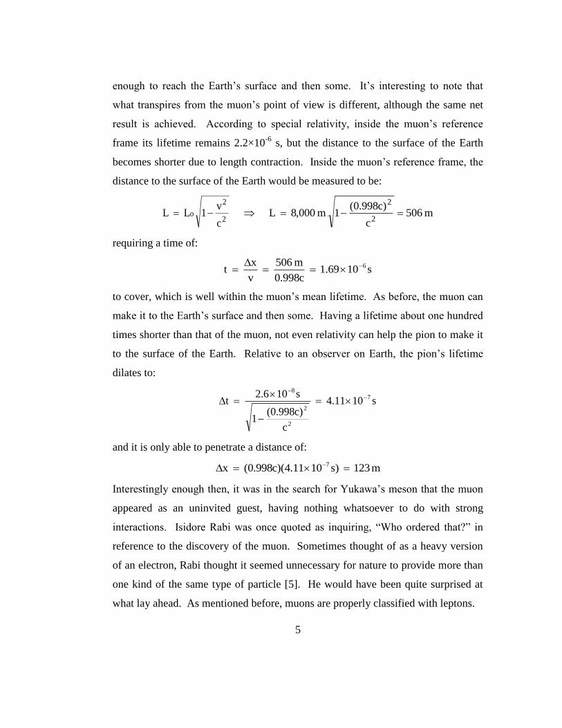
Figure 1.4: No secret chambers to be found would imply solid rock all the way

through the pyramid and relatively uniform muon counts throughout the scanned

area [6].

Figure 1.5: A secret chamber in the pyramid would be revealed by a higher than

usual muon count within the scanned area. The circled area in the figure reveals

how the presence of a hollow volume would be detected by allowing more muons

to pass through in that direction [6].

11

After reading this account, I couldn’t help but be reminded of the Michelson-

Morley experiment. Michelson and Morley came up with a revised, elaborate, and

clever method to measure the speed of the Earth through the ether, which was

hypothesized to be the medium through which light propagates. If the ether existed

and could be used as an absolute reference frame, then differences in the speed of

light should have been able to be detected in their experiment. They were, of

course, able to detect no difference in the speed of light, and one would imagine

that they were probably somewhat disappointed with their anticlimactic result.

Anticlimactic or not, Michelson and Morley’s null result is one of the most

important experimental results in physics and played a role in shaping and

supporting Einstein’s theory of special relativity. While the underpinnings of

theoretical physics did not hinge on Alvarez’s results, there are certainly analogies

to be made. His muon photography experiment was absolutely beautiful, and it

would have been a picture perfect end to the story had a pot of gold been found at

the end of the rainbow, but the fact is that there exists no hidden chambers in the

pyramid investigated. When people would say to Alvarez, “So you didn’t find any

chambers”, his response was, “No, we found that there are no chambers.” Around

the same time, in 1968, Luis Alvarez won the Nobel Prize in Physics “For his

decisive contributions to elementary particle physics, in particular the discovery of

a large number of resonant states, made possible through his development of the

technique of using hydrogen bubble chambers and data analysis [6].”

An interesting application of muon tomography using cosmic ray muons

involves the pursuit of detecting nuclear (high-Z) material. After being developed

by Christopher Morris in 2001, Los Alamos National Lab started to explore the use

of MT to detect nuclear contraband at our nation’s ports and borders in 2003 [7]-

[11]. The threat of nuclear contraband being smuggled across international borders

is ever present, and new ways of detecting such contraband are important to

national security interests. Muon tomography offers advantages over current

12

detection systems through its ability to discriminate high-Z material from a lower-Z

background, thereby making it more difficult to shield special nuclear material

(SNM) [16]. In fact, results of simulations that I will present later suggest that

attempting to shield uranium with lead that would make it very difficult to detect

using current systems could cause it to show up slightly stronger (than with no

shielding) in an image created using muon tomography. Furthermore, if an

efficient muon tomography detection based system could be brought to market, it

would not only offer certain detection advantages, but may also be more affordable

than current systems which are not able to take advantage of a free imaging source.

As mentioned previously, to date muon tomography makes use of advanced

detectors that have been developed at CERN. Drift tubes have been used by

Decision Sciences Corporation in the development of a muon tomography system

designed to detect nuclear contraband. In 1992, Georges Charpak won the Nobel

Prize in physics for the invention of this kind of detector [12]. Our research group

has been funded by the Department of Homeland Security to develop a muon

tomography system using GEM detectors, developed by Fabio Sauli. An advantage

of using GEM detectors is that they are capable of better spatial resolution than

drift tubes are. A disadvantage is that because they are a relatively new technology,

very large (>1 m) GEM detectors have yet to be manufactured, making it very

difficult to currently image large volumes using them. Although muons have high

penetrating properties, they do interact with matter to some degree via Coulomb

scattering. Muons are scattered more by atoms with large atomic numbers (high-Z

material) than they are by atoms with small atomic numbers. By using detectors

that can track incoming and outgoing velocity vectors of muons and using an

algorithm that can calculate the position that a deflection occurred along with a

scattering angle, material can be imaged using four dimensional data. Three of the

dimensions locate a point in space where material exists, and the fourth dimension

(scattering angle) indicates the density of the material present. A Point Of Closest

13

Approach (POCA) reconstruction method is one such algorithm that finds the

intersection of incident and exiting muon trajectories and assigns a color coded

image to the voxel (a small volume containing the point of interaction)

commensurate with the scattering angle [7], [16]. This is the type of reconstruction

method our research group uses. Another algorithm involves a Maximum

Likelihood / Expectation Maximization (ML/EM) reconstruction method that

borrows much from techniques used in medical imaging, but incorporates the

statistics of muon scattering [10]. One challenge to overcome in developing a

muon tomography system aimed at detecting nuclear contraband is that viable

systems should be able to detect SNM within a few minutes, and there is no way to

increase the flux of cosmic ray muons. A great reconstruction algorithm could play

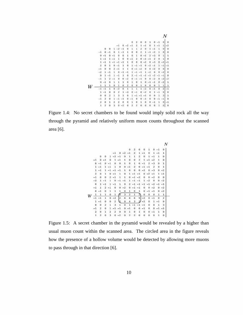
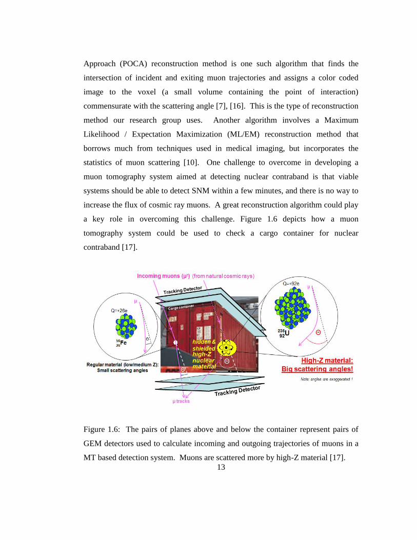
a key role in overcoming this challenge. Figure 1.6 depicts how a muon

tomography system could be used to check a cargo container for nuclear

contraband [17].

Figure 1.6: The pairs of planes above and below the container represent pairs of

GEM detectors used to calculate incoming and outgoing trajectories of muons in a

MT based detection system. Muons are scattered more by high-Z material [17].

14

Because our muon tomography system employs GEM detectors, and accounting for

their use primarily drove the designs of the two prototype stations I designed and

built, the following section explains the basics of how they work.

1.3 Gas Electron Multiplier (GEM) Detectors

Gas Electron Multiplier (GEM) detectors are micro-pattern gas detectors

used for the detection of charged particles [13]. Each GEM detector has five basic

components: a honeycomb frame, a drift cathode, foils (referred to as GEM foils),

a readout, and a gas mixture which fills the volume of each sealed detector [18].

Fast moving charged particles passing through a detector first ionize the gas filling

it in the drift region.

Figure 1.7: Cross section of a triple-GEM detector illustrating the electron

multiplication that occurs within the gas-filled detector [19].

The freed electrons are then accelerated through a series of GEM foils (usually two

or three) that have a potential difference across them, further ionizing the gas and

producing an avalanche of electrons (fig. 1.7) [19]. This is the electron

15

multiplication that occurs in the gas-filled detectors that their name (Gas Electron

Multiplier) implies, and it is the means by which the original signal (in this case a

charged particle ionizing gas) is amplified into a measurable current. The

avalanche of electrons induces a charge in the readout and thereby produces a

current which reveals the position that the fast moving charged particle crossed the

detector. Detectors that use two GEM foils for signal amplification are called

double-GEM detectors, and those that use three are called triple-GEM detectors.

Each detector has a honeycomb frame which serves to provide strong

structural integrity while minimizing the amount of material required to do so

(hence the honeycomb geometry). Minimizing the amount of material used for the

structural support of each detector is important because it can potentially interfere

with the particles sought to be detected [18].

The drift cathode found in each detector is made of kapton and is coated on

one side with copper. Kapton is a polymer foil with very strong insulating

properties manufactured by the Du Pont Company [20]. It’s only about 50 μm

thick, and the copper coating is only about 5 μm thick. The side of the drift

cathode that is not coated is attached to the honeycomb frame. A negative electric

potential is applied to the drift cathode which serves to attract the positive ions

created in the ionization process described above. This is important because it

helps to prevent positive ions from recombining with freed electrons before they

can be propagated downward to the readout [18].

Each GEM foil used in a detector is also made of kapton and is coated with

copper on both sides. Again, the kapton is about 50 μm thick and the copper

coating on each side is about 5 μm thick. Each foil is pierced by a regular array of

chemically etched holes that are about 140 μm apart (this is why GEM detectors are

referred to as micro-pattern gas detectors). The holes have a conical shape to them,

and the technique used to etch the holes and to give them their desired shape was

16

developed at CERN (fig. 1.8-9). The outer diameter of the conically shaped holes

is 70 μm, and the inner diameter is 50 μm [14], [21].

Figure 1.8: Magnified view of the micro-pattern holes etched into each GEM foil

[14], [21].

In a triple-GEM detector, the voltage applied across each GEM foil is typically

between 400 and 500 volts. The holes piercing each foil have their conical shape

for two reasons: to help prevent unwanted and potentially very damaging sparking

from one side of the foil to the other, and to help concentrate the electric field lines

that fill each hole which serves to amplify the original signal [13]. Free electrons

caught in the field filling these holes are accelerated to high enough speeds to

further ionize the gas filling each detector, and the number of free electrons able to

make it to the readout and produce a measurable current is multiplied. Before

being deployed, GEM foils must be stretched and framed. Within a detector it is

critical that GEM foils maintain a uniformly flat surface area to function properly

[13].

17

Figure 1.9: The conical shape of the holes etched into each GEM foil helps to

concentrate the electric field lines filling them. Here, electric field lines (red) and

equipotential lines (green) are shown [14], [21].

A readout must be placed at the bottom of each detector to measure the

amplified signal of an interaction (gas being ionized by a cosmic ray muon in our

case) and to determine the position at which the interaction occurred. The readouts

used for the detectors in the muon tomography station prototypes I designed have

two dimensional readout strips with a 400 μm pitch and analog readout and can

reach a position resolution of 50 – 80 μm for muons with perpendicular incidence

[21]. The two dimensional readout strips can be thought of as x-y, x-z, or y-z strips

depending on the choice of coordinate system and the readout’s placement within

it.

The choice of gas used to fill each detector is a critical one. The gas should

be relatively easy to ionize, and electron avalanching should be obtainable in a

relatively low electric field because they pose less danger to the detector. The gas

should recover quickly from electron avalanching and should be non-corrosive to

the GEM foils used in each detector. It turns out that the noble gasses are ideal

18

candidates to meet all of these criteria, with those having higher atomic numbers

being preferred. Because xenon and krypton are so expensive, argon is the most

cost effective choice. However, there is a problem with the use of pure argon. The

only way for argon to return to ground state is by emitting a photon which can

cause secondary ionization on the GEM foils themselves, thereby producing a false

signal. To overcome this problem, a polyatomic molecule can be introduced to the

gas because they can be very useful in preventing these kinds of secondary

ionizations. Carbon dioxide is an excellent choice, and a mixture that optimizes all

of the desired characteristics is seventy percent argon and thirty percent carbon

dioxide (Ar/CO2 70:30). Gas composed of this mixture of argon and carbon

dioxide is cost-efficient, relatively easy to ionize, facilitates electron avalanching in

a relatively low electric field, recovers quickly from electron avalanching, and is

non-corrosive to metal inside each detector [18].

The detectors used in the prototype stations I designed are triple-GEM

detectors using 30 cm × 30 cm GEM foils, yielding an active area of 900 cm2 for

each detector. The thickness of each detector is about 1.3 cm, from the top of the

readout to the top of the honeycomb frame placed over the drift cathode. In our

application (muon tomography) of the triple-GEM detectors, cosmic ray muons are

the fast moving charged particles ionizing the Ar/CO2 (70:30) gas mixture in the

detectors, and the position that they cross a detector can be read out to a resolution

of 50 – 80 μm for muons with perpendicular incidence.

19

Chapter 2 Muon Tomography Station Prototypes

2.1 Muon Tomography Station Prototype I

One of the long term goals of our research group is to design and

commission large scale muon tomography stations that can be used to image cargo

containers at our nation’s ports and prevent the smuggling of nuclear contraband

into our country more efficiently and less expensively than is currently done.

When I first joined our group in 2008, we were in the earliest phases of this

endeavor. At that time, we had run exhaustive simulations which suggested that

our long term goal of developing a muon tomography station using GEM detectors

was quite feasible. By early 2009 we were getting ready to collect real data from

physical detectors to verify predictions made by our simulations and to refine our

imaging techniques. Ultimately, our group would need to design an imaging

station that could accommodate detector stacks on at least four sides of an imaging

volume. A minimum of two detectors are required in a detector stack because each

detector reads out a point in space where a muon crossed it, and it takes at least two

points to define a line (the muon’s incoming or outgoing trajectory). If more than

two detectors are used in a stack, then lines of best fit can be calculated to

determine trajectories. The reality in 2009 was that we were going to have fewer

than eight detectors at our disposal, which meant that even if we had a station that

could accommodate detector stacks on four sides, we would only be able to

actually employ detector stacks on the top and bottom of our imaging volume. A

decision was therefore made that our first muon tomography station (MTS)

prototype would be both simple and elegant and able to accommodate detector

stacks on the top and bottom of an imaging volume only. This kind of design could

be produced quickly and allow for the collection of real data by the fall of 2009. I

was tasked to design and build our group’s prototype I station accounting for the

20

use of GEM detectors with 30 cm × 30 cm active areas that are 1.3 cm thick during

the summer of 2009. In 2010 I would design and build our group’s MTS prototype

II, capable of mounting detector stacks on four sides of an imaging volume and the

subject of the following section.

I decided that the simplest way to implement a design accommodating top

and bottom detector stacks only would be to take advantage of fixation holes that

readouts we use have drilled into them during manufacturing. Each readout has

three fixation holes that are a quarter inch in diameter in close proximity to three of

the four corners where each detector is attached to it. I pursued a design that

employed quarter inch stainless steel threaded rods emanating upward from a base

support plate made of aluminum. Detectors would be supported by the rods

directly, which would pass through the fixation holes in each readout. Support for

the detectors (and readouts) on three sides would be sufficient due to their low

mass and to the fact that there would be no excess mass, or mass concentration,

close to the corner with no support. Using three support rods would work fine for

the detectors, but would not be a practical solution to support the target plate which

would be placed between the top and bottom detector stacks. The target plate is the

element in my design that supports whatever material we want to image. It needs

to be massive or strong enough to support high mass objects that can be placed

anywhere in the imaging volume. A fourth support rod would definitely be needed

to support the target plate, and I implemented a fourth rod for this purpose that

extended beyond the area of each detector and readout. All detectors and the target

plate would share three quarter inch stainless steel support rods, and the target

plate, made of aluminum 3/8 inch thick, would have a fourth support rod passing

only through it to provide the extra support needed.

The primary structural components of our MTS prototype I consisted of a

base plate used to support four ¼-20 threaded stainless steel rods, and a target plate.

The base plate was made of aluminum and designed with cylinders (also

21

aluminum) emanating up from where the steel rods screw into it. The steel support

rods could screw deeper into the cylinders than the thickness of the base plate

would allow, making them more stable. 6061-T6 aluminum alloy was used to

machine all components made of aluminum in prototypes I and II. Machinists in

our shop recommended the use of this kind of aluminum due to its strength while

still being easy to machine. Other components used to mount the detector stacks

and target plate follow: ¼ inch washers one inch in diameter (placed underneath

readouts to distribute pressure), ¼ inch heavy hex nuts (tightened down on top of

the cylinders of the base plate to add stability), 7/8 inch stainless steel coupling nuts

(used to support the target plate and the bottom detector assembly of the top

detector stack), ½ and ¾ inch nylon spacers (used to quickly and accurately

establish desired separation distances between detectors in a stack), and nickel anti-

seize lubricant for the aluminum base plate / stainless steel rod interface (used to

prevent the aluminum and steel from locking up). Appendix A contains directions

for assembly. Following are images of our MTS prototype I, starting with some

simulated images made using SolidWorks (fig. 2.1-2) and concluding with various

images of the actual prototype (fig. 2.3-7). SolidWorks is a 3D CAD (Computer-

Aided Design) design, analysis, and product data management software package

developed by Dassault Systèmes SolidWorks Corporation [22]. Both MTS

prototypes I and II were modeled using this software during the various phases of

their designs to test for feasibility and to make final improvements before

production.

22

Figure 2.1: Top view of MTS prototype I using SolidWorks. From this

perspective, simulated elements of the top detector assembly in the top stack are

readily seen including gassiplex cards (green), Panasonic adaptors (red), the section

where high voltage is applied (blue), the readout (brown), the GEM detector (gold),

and a portion of the target plate (silver). In the portion of the target plate visible,

one can see the hole through which the fourth support rod would pass through it.

All dimensions shown are in inches.

Figure 2.2: Three dimensional view of our MTS prototype I with top and bottom

detector stacks using SolidWorks. All main elements of the prototype are visible,

along with some material to be imaged on the target plate.

23

Figure 2.3: Actual base plate used in our MTS prototype I. Its dimensions are

20 in × 22 in × ¾ in. The cylinders have an outer diameter of ¾ in, an inner

diameter of ¼ in, and a height of 3.0 in. Steel support rods screw into them 1.5 in

deep. The engraving reads “Dr. Marcus Hohlmann / Florida Institute of

Technology / High Energy Physics.”

Figure 2.4: The target plate used in our MTS prototype I. Its dimensions are

20 in × 22 in × 3/8 in. The engraved square denotes the boundaries of the imaging

volume, and the three holes visible by the top left, bottom left, and bottom right

corners of the square align with the three fixation holes in each readout. The fourth

hole in the target plate used by the fourth support rod which passes through the

target plate only is in the upper right hand corner of the image and is hard to make

out due to various reflections. All holes are ¼ inch in diameter.

24

Figure 2.5: MTS prototype I loaded with mock readouts and mock material to be

imaged. Nylon spacers can be seen to separate the readouts at uniform distances.

Figure 2.6: MTS prototype I with mock readouts and imaging material from

another perspective. The readout at the top of the top stack was an actual readout

that had been damaged. One can see the fourth support rod going through the

target plate only.

25

Figure 2.7: Fully commissioned MTS prototype I collecting data at CERN. Note

that two GEM detectors are being used in each detector stack, and a small block of

lead is being imaged. The damaged readout is able to serve as the target plate here

used to image material [23].

26

2.2 Muon Tomography Station Prototype II

Our MTS prototype I served its purpose well and allowed for the first

collection of real data from GEM detectors used to image material. As new

detectors were being commissioned and becoming available to use, our focus

turned to a prototype II design that would be able to accommodate detectors on

four sides of an imaging volume in the form of a cube about a cubic foot in size.

During the first several months of 2010, I worked on our prototype II design using

SolidWorks, and over the summer I built and commissioned it.

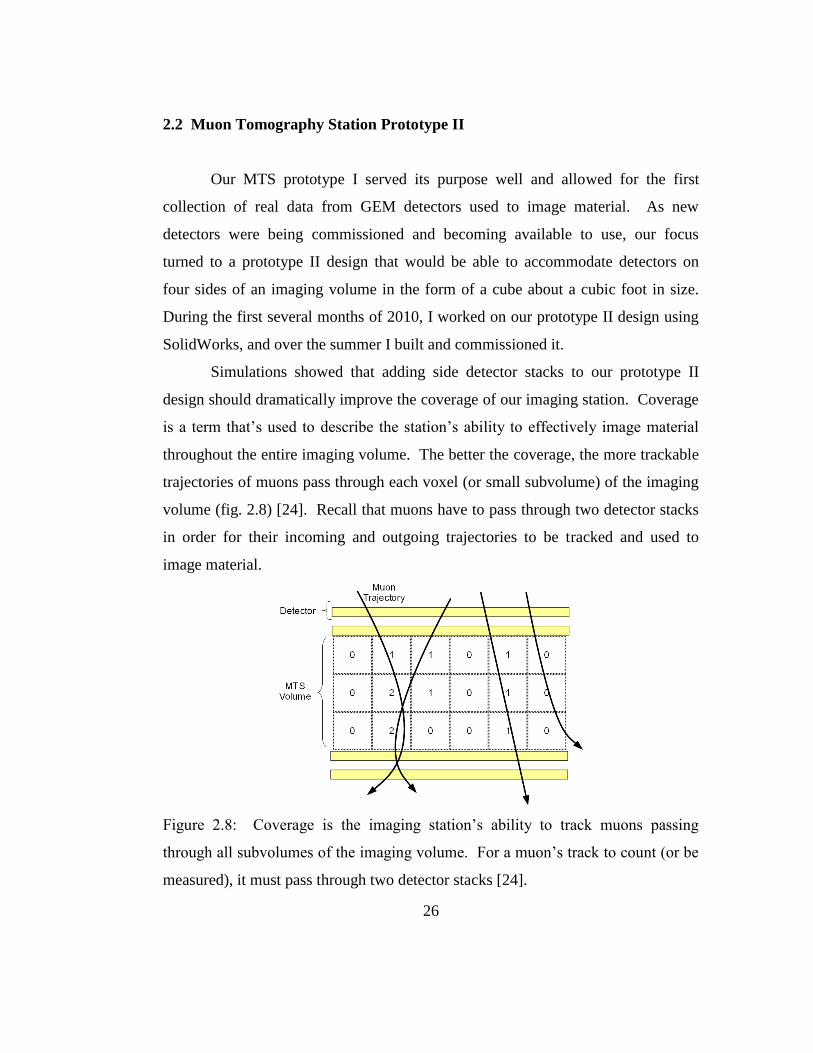
Simulations showed that adding side detector stacks to our prototype II

design should dramatically improve the coverage of our imaging station. Coverage

is a term that’s used to describe the station’s ability to effectively image material

throughout the entire imaging volume. The better the coverage, the more trackable

trajectories of muons pass through each voxel (or small subvolume) of the imaging

volume (fig. 2.8) [24]. Recall that muons have to pass through two detector stacks

in order for their incoming and outgoing trajectories to be tracked and used to

image material.

Figure 2.8: Coverage is the imaging station’s ability to track muons passing

through all subvolumes of the imaging volume. For a muon’s track to count (or be

measured), it must pass through two detector stacks [24].

27

With top and bottom detector stacks only, there are many possible ways for a muon

to pass through the imaging volume without passing through both top and bottom

detector stacks. By adding detector stacks on two more sides of the imaging

volume (covering four of six sides of the imaging volume), muons have fewer

opportunities to avoid detection. With four sides of the imaging volume covered,

muons crossing the top detector stack and either side detector stack can be tracked,

and muons crossing either side detector stack and the bottom detector stack can be

tracked, in addition to those crossing top and bottom detector stacks. Muons

crossing both side detector stacks could also be tracked, but such an event would be

less likely. Muons have the highest probability of impacting at an angle of 30°

from the vertical at sea level. One might wonder why all six sides of the imaging

volume aren’t covered to maximize coverage. Two sides of the volume are left

uncovered because in the final version, cargo containers must pass through the

imaging volume. Sealing off the volume would make impractical the use for which

the station was created.

An imaging station with detector stacks on four sides should be a big

improvement over the prototype I station, but the design of such a station would

have to be very different. Threaded steel rod worked beautifully for a station with

top and bottom detector stacks only, but steel rod could not be effectively used to

mount side detectors. Since steel rod could not be used, each detector would need

its own support plate which would be mounted in a different kind of framework.

Detectors would have to be mounted to their support plates via the fixation holes in

each detector’s readout. Furthermore, support plates would have to be big enough

to allow for the space needed by electronics and other various components, such as

gas lines, used by each detector. Since the support plates would be larger than the

detectors themselves, if they were brought together in such a way as to make four

sides of a box, the active area of each GEM detector would not overlap. Active

areas of each detector coming together must overlap and define a closed volume to

28

improve the coverage of the station. This problem was solved by overlapping the

detector support plates themselves. Overlapping the support plates would allow the

active areas of each GEM detector to overlap and would define a volume closed on

four sides by active areas of GEM detectors.

Figure 2.9: PVC plate used to support GEM detectors and their readouts. The

support plates have dimensions of ¼ in × 19 in × 26 in. PVC is cut out of the

support plate where detectors will be located so that the plate itself does not

interfere with a muon’s trajectory. The cut-outs are 13 in × 13 in.

Figure 2.10: Simulated view of a detector assembly mounted to its support plate

using SolidWorks. Elements of the detector assembly shown are APV chip hybrid

cards (green), the section where high voltage is applied (blue), the readout (brown),

the GEM detector (gold), and cylinders representing sites for gas inlet and outlet.

29

Figure 2.11: Geometry of overlapping detector support plates in such a way as to

allow the active areas of each GEM detector to define a closed volume. A

simulated target plate with material to be imaged is also shown. The defined

imaging volume is about 31 cm3, or about a cubic foot, and the closest detectors

can be brought together is about 1.5 in due to physical limitations.

Once it was determined what the geometry of the support plates must be to

maximize coverage, I tried to imagine an imaging station, or framework, built

around that geometry. I wanted the design to be a clean and efficient solution to

mounting the support plates in their required geometry fixed in space. I had to

meet the following specific design requirements, but was given flexibility in how I

did so: the detector geometry shown in figure 2.11 had to be accommodated, I had

to allow for variable, discrete spacing of detectors in multiples of ¼ inch, PVC

support plates had to account for the space required by various hardware

components needed to support each detector (fig. 2.9-10), and the station had to be

portable (able to be broken down). After working out the problem on paper, I used

SolidWorks to test my solution. My prototype II design consisted of extruded

angles and T-bars made of 6061-T6 aluminum alloy welded together to make four

quadrants (fig. 2.12-2.15). The four quadrants of the framework were bound

together by smaller extruded angles screwed into it used to support top and bottom

detector stacks, as well as support brackets connected to them using nuts and bolts

30

for maximum stability. The extruded angles and T-bars used to make each

quadrant of the imaging station had holes drilled in them spaced a quarter of an

inch apart so that detectors in each stack could be arranged at various separation

distances, meeting that design requirement. Following are selected images of the

MTS prototype II I designed (fig. 2.16-2.20) and of some of its components. The

simulated images were made using SolidWorks. Complete drawings of all the

components used to construct both prototypes in PDF and SolidWorks files are

available on the FIT T3 Open Science Grid cluster under the account “g4hep”:

[email protected]; file path geant4/examples/mytestapps/lenny/

MTS Prototypes.

Figure 2.12: An extruded angle used to construct quadrant one of the prototype II

imaging station. The L shape is 1.5 in × 0.75 in and is 0.125 in thick, and the angle

itself is 15.5 in long. The holes are 0.113 inches in diameter, are 0.25 in apart, and

are used to fixate the PVC detector support plates. Another extruded angle is used

in quadrant one that is 26.5 in long.

Figure 2.13: A T-bar used to construct quadrant one of the prototype II imaging

station. The T shape is 1.5 in × 1.5 in and is 0.188 in thick, and the bar itself is

15.5 inches long. The holes are 0.113 inches in diameter, are 0.25 in apart, and are

used to fixate the PVC detector support plates.

31

Figure 2.14: Quadrant one of our MTS prototype II imaging station. Elements one

and two are referenced in figure 2.12, and elements three and four are like that

shown in figure 2.13. Element five is simply an aluminum base plate used for

support, and element six is an extruded angle with no holes also used to support the

framework. Note that the vertical extruded angle and T-bar have twin sets of holes.

One set is used to screw into extruded angles that support detector assemblies in

top and bottom detector stacks, and the other set is used to fixate the PVC in those

stacks. The sets of twin holes have the same dimensions as those mentioned in the

two previous figures and are separated by half an inch. All elements shown are

welded together to form a solid and stable assembly.

2

3

6

5

1

4

32

Figure 2.15: Quadrants one and two of our MTS prototype II imaging station.

Quadrant two is composed of the same fundamental elements as quadrant one, and

they are arranged to accommodate the geometry shown in figure 2.11. In a similar

fashion, quadrants three and four are constructed.

Figure 2.16: Simulated MTS prototype II imaging station complete with all four

quadrants, four detector stacks, and target plate with material to be imaged. The

black elements represent scintillators used to trigger on trackable muon trajectories,

and each detector stack has one. The completed station is approximately 47 inches

long by 29 inches wide by 42 inches high.

33

Figure 2.17: Assembled MTS prototype II in Florida Tech’s machine shop shortly

after its construction was completed in June 2010. The station is loaded with PVC

support plates that will be used to secure GEM detectors and scintillators, along

with their supporting electronics.

Figure 2.18: Assembled MTS prototype II in Florida Tech’s High Energy Physics

Lab A. Along with PVC support plates, the station is also loaded with target plates

secured by C-clamps and mock material to be imaged.

34

Figure 2.19: Partially loaded MTS prototype II at CERN. Top and bottom detector

stacks are fully loaded, but side detectors have not been mounted yet. A target

plate with material to be imaged is also missing.

Figure 2.20: Fully loaded MTS prototype II in Florida Tech’s High Energy Physics

Lab A. Detector stacks are mounted on all four sides, and one can see the material

being imaged in the center of the imaging volume.

35

Chapter 3 MTS Prototype II Simulated Scenarios

3.1 Photon Attenuation Calculation

The primary materials used for nuclear fission weapons are U-235 and Pu-

239 [25]. In the simulations that follow in the next section, I chose to test the

effectiveness of our imaging station to detect U-235 encased in lead shielding.

Current detection systems are designed to detect high energy photons emitted from

nuclear contraband. The most probable gamma emitted by U-235 has an energy of

186 keV, and over 92% of all gammas emitted have an energy equal to or less than

this value [26]. By looking at the photon mass attenuation length for lead given a

photon energy of 186 keV, one can calculate the thickness that a box made of lead

would need to have in order to shield 99.9% of all photons with that energy.

Figure 3.1: The photon mass attenuation length is given for various elements as a

function of photon energy [27].

36

The formula used for such a calculation is as follows:

x

oeI I(x) [27]

where: I(x) is the intensity of the photon remaining after traveling a distance x in

cm through the material;

oI is the initial intensity of the photon;

ρ is the density of the material traversed in g/cm3;

λ is the photon mass attenuation length, or mean free path, given the

material traversed and energy of the photon in g/cm2.

The density of lead is ρ = 11.34 g/cm3, and the photon mass attenuation length for a

gamma of energy 186 keV traveling through lead is λ = 0.8 g/cm2 (fig. 3.1) [27].

Therefore, to calculate the thickness of lead needed to absorb 99.9% of all gammas

with energy 186 keV we have:

x

oeI I(x) 8.0

x34.11

oo eI I 001.0

0.8

11.34x- )001.0(ln

mm 4.87 cm 0.487 11.34-

(0.001)ln 0.8 x

Therefore, a lead box of thickness 5 mm would be capable of shielding over 99.9%

of over 92% of all gammas emitted from U-235. Such a shield would probably be

effective at smuggling U-235 given current detection systems. The following

section will show that such a shield would not only be ineffective given a muon

tomography based detection system, but could in fact make the U-235 stand out

even more.

37

3.2 Analysis of Simulated Scenarios

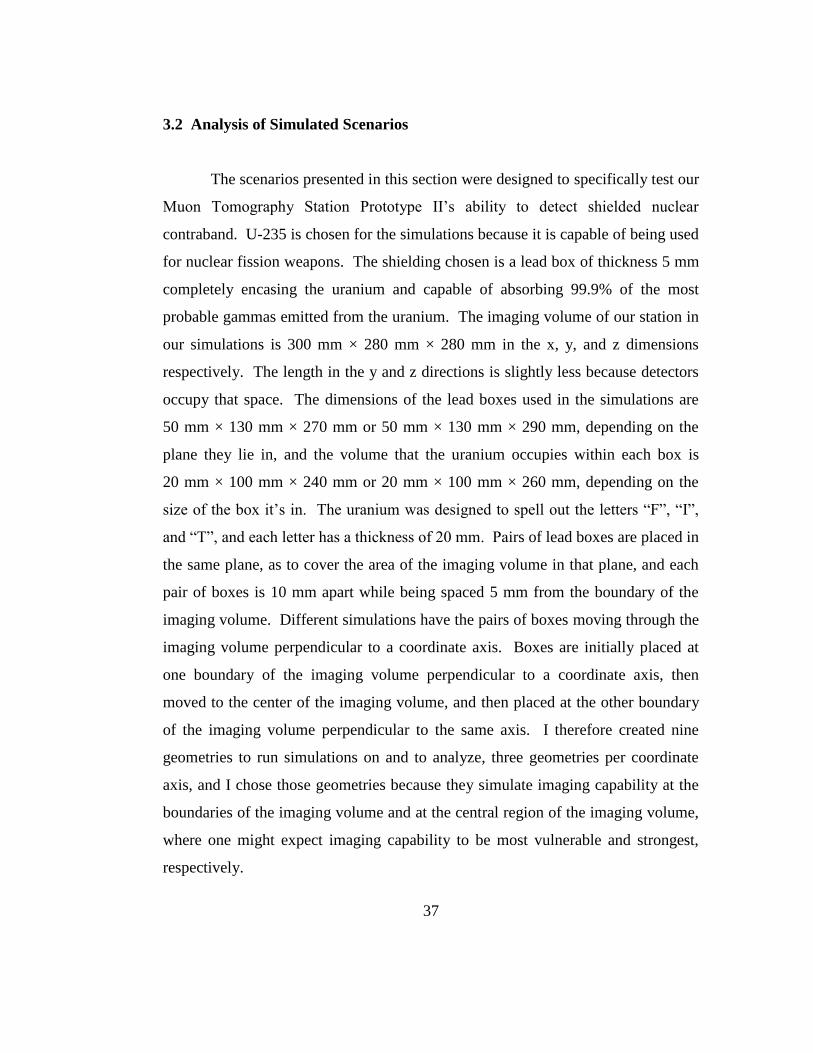
The scenarios presented in this section were designed to specifically test our

Muon Tomography Station Prototype II’s ability to detect shielded nuclear

contraband. U-235 is chosen for the simulations because it is capable of being used

for nuclear fission weapons. The shielding chosen is a lead box of thickness 5 mm

completely encasing the uranium and capable of absorbing 99.9% of the most

probable gammas emitted from the uranium. The imaging volume of our station in

our simulations is 300 mm × 280 mm × 280 mm in the x, y, and z dimensions

respectively. The length in the y and z directions is slightly less because detectors

occupy that space. The dimensions of the lead boxes used in the simulations are

50 mm × 130 mm × 270 mm or 50 mm × 130 mm × 290 mm, depending on the

plane they lie in, and the volume that the uranium occupies within each box is

20 mm × 100 mm × 240 mm or 20 mm × 100 mm × 260 mm, depending on the

size of the box it’s in. The uranium was designed to spell out the letters “F”, “I”,

and “T”, and each letter has a thickness of 20 mm. Pairs of lead boxes are placed in

the same plane, as to cover the area of the imaging volume in that plane, and each

pair of boxes is 10 mm apart while being spaced 5 mm from the boundary of the

imaging volume. Different simulations have the pairs of boxes moving through the

imaging volume perpendicular to a coordinate axis. Boxes are initially placed at

one boundary of the imaging volume perpendicular to a coordinate axis, then

moved to the center of the imaging volume, and then placed at the other boundary

of the imaging volume perpendicular to the same axis. I therefore created nine

geometries to run simulations on and to analyze, three geometries per coordinate

axis, and I chose those geometries because they simulate imaging capability at the

boundaries of the imaging volume and at the central region of the imaging volume,

where one might expect imaging capability to be most vulnerable and strongest,

respectively.

38

GEANT4 (GEometry ANd Tracking) is a C++ toolkit designed to run

particle physics simulations, and the code for the simulations I ran had already been

written by other members of my research group [28]. Using my group’s code to

run the simulations I designed required me to learn how to modify the

configuration file responsible for generating the specific material used in each

simulation, as well as their geometry. Within the configuration file used for each

simulation I also established a 9 m2 CRY (Cosmic RaY) plane centered above the

imaging volume [29], [30]. A CRY plane is a surface from which GEANT4

generates particles, cosmic ray muons in our case. Each cosmic ray muon

generated is called an event, and the number of events run, or cosmic ray muons

generated, can also be set in the configuration file. Therefore, the simulations are

run in event space, and it is important to know how many events correspond to the

passage of time in the real world. One important factor to consider in our imaging

station is how well it can image material in a given time interval. Transforming

from the number of events run in event space to the passage of time in the real

world is easily done given the cosmic muon flux at sea level, which is 1x104 events

per square meter per minute. The following equation can then be used to determine

how many events, or muons generated, correspond to the passage of a specified

amount of time.

2

4

mmin

events 1x10

1

m (area)min (time) 2 = number of events

For my simulations, I chose to produce plots for exposure times of 1 minute,

4 minutes, 10 minutes, 60 minutes, and 600 minutes. The number of events that

corresponds to the above exposure times is calculated below.

2

4

mmin

events 1x10

1

m 9min 1 2 = 90,000 events

39

2

4

mmin

events 1x10

1

m 9min 4 2 = 360,000 events

2

4

mmin

events 1x10

1

m 9min 10 2 = 900,000 events

2

4

mmin

events 1x10

1

m 9min 60 2 = 5,400,000 events

2

4

mmin

events 1x10

1

m 9min 600 2 = 54,000,000 events

Each simulation was run with 54,000,000 events, corresponding to an elapsed time

of 10 hours, and to help minimize the time required to run a simulation, 50

simulations were run in parallel, each with 1,080,000 events, and their results were

concatenated into a single file compiling the results of 54,000,000 events. Running

50 simulations on 50 CPUs in our computing cluster simultaneously went much

faster (about 50 times) than running a single simulation on a single CPU with 50

times the number of events. Furthermore, because of the random nature in which

GEANT4 generates muons to correspond with reality, concatenating the results of

50 simulations with 1,080,000 events each is statistically equivalent to looking at

the results of a single simulation producing 54,000,000 events. The concatenated

file for each simulation contained four dimensional data for each trackable event.

The data consisted of three spatial coordinates and a scattering angle, denoting the

location within the imaging volume that a muon interacted with material and the

angle at which it was scattered. Recall that in order for the event to be trackable,

the muon has to cross a detector stack before and after interacting with material in

the imaging volume. It turned out that for a 9 m2 CRY plane centered above an

imaging volume of approximately a cubic foot, 54,000,000 generated events would

40

translate to about 657,000 trackable events. That is around 657,000 of 54,000,000

generated events ended up passing through the imaging volume, interacting with

material, and passing through two detector stacks. The concatenated files for each

of the nine scenarios simulated all contained very close to 657,000 data elements,

the average being 657,348. This meant that for a concatenated data file, 657,348

elements would correspond to 10 hours of elapsed time in the real world, and

proportionalities could be used given the number of events calculated previously to

calculate how many data elements would correspond to the other times. For

example, if 90,000 of 54,000,000 events correspond to 1 minute of elapsed time,

then 1,096 of 657,348 concatenated data elements would also correspond to 1

minute of elapsed time, etc.

This is important to know because the concatenated data file for each

simulation is called by the ROOT configuration file to perform analysis on the

results of each simulation [31]. ROOT (Rapid Object-Oriented Technology) is a

C++ data analysis framework used to perform analysis by the particle physics

community, and the code to perform the analysis of our group’s simulations had

already been written by other members. However, I modified the code to allow for

a variable number of data to be used from the concatenated data file, making it

possible to view what different time exposures would look like without having to

run more simulations. The desired number of data to be analyzed from the

concatenated data file is entered in the ROOT configuration file, along with a range

of scattering angles to govern each plot generated. In addition to the lead and

uranium included in each scenario, the imaging volume was filled with air, and

scattering angles below 3 degrees were not shown, while scattering angles above 8

degrees were shown as 8 degrees. This range was chosen to slightly improve the

quality of images produced in the analysis. I used ROOT to analyze the output of

my simulations run and to produce images of what our station should be able to

produce for a given scenario. In the images of my analysis that follow, all data in

41

the perpendicular coordinate is collapsed into the plane shown, and degrees shown

refer to the scattering angle of muons passing through material. Here images

produced given an elapsed time of 10 hours are shown; images for elapsed times of

4 minutes, 10 minutes, and 60 minutes for each scenario are included in appendix

E. The configuration files I created for each scenario are included in appendix C,

and the code I modified to run my Root analysis is included in appendix D.

I used HepRApp to visualize the geometry of each scenario I created so that

any errors could be quickly spotted and then corrected before running my

simulations [32]. HepRApp, the original HepRep Data Browsing Application, is a

Java application that was developed to let physicists visualize particles interacting

with matter (HepRep is a generic interface definition for high energy physics event

display representables).

In each simulation, the center of the imaging volume is defined to be at the

origin of a Cartesian x-y-z coordinate system. Recall that detector stacks cover

four sides of the six-sided volume. The x-axis passes through the open ends of the

imaging volume, while the y-axis is perpendicular to two detector stacks, and the z-

axis is perpendicular to two detector stacks. The x and y axes are in the horizontal

plane (parallel to the surface of the Earth), which makes z the vertical axis. Note

that in each simulation there are three detectors in top and bottom detector stacks,

and there are two detectors in both side stacks (fig. 3.2). Also note that the

simulated resolution in each GEM detector is perfect.

Figure 3.2: Detector geometry and coordinate axes used in each simulation [33].

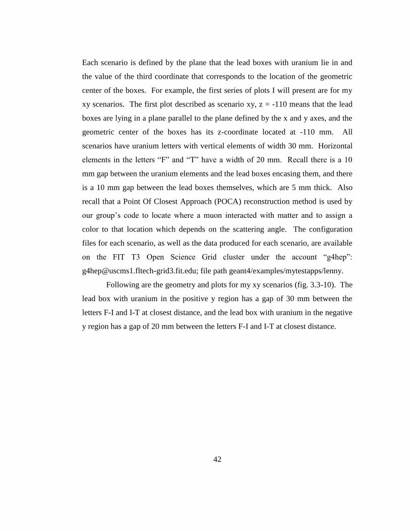
42

Each scenario is defined by the plane that the lead boxes with uranium lie in and

the value of the third coordinate that corresponds to the location of the geometric

center of the boxes. For example, the first series of plots I will present are for my

xy scenarios. The first plot described as scenario xy, z = -110 means that the lead

boxes are lying in a plane parallel to the plane defined by the x and y axes, and the

geometric center of the boxes has its z-coordinate located at -110 mm. All

scenarios have uranium letters with vertical elements of width 30 mm. Horizontal

elements in the letters “F” and “T” have a width of 20 mm. Recall there is a 10

mm gap between the uranium elements and the lead boxes encasing them, and there

is a 10 mm gap between the lead boxes themselves, which are 5 mm thick. Also

recall that a Point Of Closest Approach (POCA) reconstruction method is used by

our group’s code to locate where a muon interacted with matter and to assign a

color to that location which depends on the scattering angle. The configuration

files for each scenario, as well as the data produced for each scenario, are available

on the FIT T3 Open Science Grid cluster under the account “g4hep”:

[email protected]; file path geant4/examples/mytestapps/lenny.

Following are the geometry and plots for my xy scenarios (fig. 3.3-10). The

lead box with uranium in the positive y region has a gap of 30 mm between the

letters F-I and I-T at closest distance, and the lead box with uranium in the negative

y region has a gap of 20 mm between the letters F-I and I-T at closest distance.

43

Figure 3.3: Geometry of shielded scenarios xy: z = -110 mm, z = 0 mm, and z =

110 mm viewed in the xy plane. The positive z axis points out of the screen.


shielded scenario xy, z = -110 mm, using POCA reconstruction with 600 minutes

exposure time viewed in the xy plane. The positive z axis points out of the screen.

44


shielded scenario xy, z = 0 mm, using POCA reconstruction with 600 minutes





45

Images of the objects at both extremes of the volume perpendicular to the z-axis

look very similar, and are much better than those at the boundaries perpendicular to

the x or y axes. Uranium shows up very well at the boundaries here, with much

better resolution than in the previous two scenarios. The resolution in the x

dimension and in the y dimension has been good in the former scenarios, but this is

the first time that those dimensions are viewed together, and the combined result is

great. These boundaries also have detectors flush up against them, which definitely

enhances imaging quality at those locations. Images at the boundaries are actually

better than in the center of the volume (z = 0 mm). In the center of the volume, the

image starts to fade at both extremes of the x-axis, probably because there are no

detectors in yz plane there. In spite of the fading, the edges of the lead boxes can

still be seen in those regions and their thickness measured close the actual value of

5 mm. In fact, the thickness of all edges of the lead boxes can be measured close to

5 mm in both dimensions. The 10 mm gap between the lead boxes can be

discerned, as well as the 10 mm gap between the uranium and the boxes encasing

them. The 30 mm gap between letters F-I and I-T at closest distance can be

measured in the positive y region, and the 20 mm gap between letters F-I and I-T at

closest distance can be measured in the negative y region. The width of the vertical

elements of the uranium letters can be measured close to 30 mm, and the width of

the horizontal elements of the uranium letters can be measured close to the actual

value of 20 mm. The resolution in both the x and y dimensions from this

perspective appears to be close to 5 mm.

46

Figure 3.7: Geometry of shielded scenario xy, z = -110 mm, viewed in the yz

plane. The positive x axis points out of the screen. The geometry of the other xy

scenarios are from this perspective as well, but the boxes are centered at z = 0 mm

and z = 110 mm.


shielded scenario xy, z = -110 mm, using POCA reconstruction with 600 minutes

exposure time viewed in the yz plane. The positive x axis points out of the screen.

47







48

All images of the objects (at both extremes of the volume along the z-axis and at

the center of the volume) look very similar to one another from this perspective.

Shielded uranium is detectable throughout the volume. These images seem hotter

than the previous set of results from the same set of scenarios because high-Z

material is spread throughout 290 mm in the x direction. From the previous

perspective, high-Z material was only spread throughout 50 mm in the z direction.

In the y dimension, the thickness of the lead boxes appears to be closer to 10 mm

than the actual 5 mm, and the gap between the lead boxes and the uranium can be

made out. The length of the uranium letters can be made out close to the actual

value of 100 mm, and the length of each lead box can be made out close to the

actual value of 130 mm. In the z dimension, the thickness of the lead boxes cannot

be made out, and the 10 mm gap between the uranium and the boxes cannot be

discerned here. The height of the uranium letters appears to be closer to 30 mm

than the actual value of 20 mm, and the height of the lead boxes appears to be

closer to 60 mm than the actual value of 50 mm.

Following are the geometry and plots for my yz scenarios (fig. 3.11-18).

The lead box with uranium in the positive z region has a gap of 20 mm between the


z region has a gap of 20 mm between the letters F-I and I-T at closest distance.

49

Figure 3.11: Geometry of shielded scenarios yz: x = -110 mm, x = 0 mm, and x =

110 mm viewed in the yz plane. The positive x axis points out of the screen.


shielded scenario yz, x = -110 mm, using POCA reconstruction with 600 minutes


50


shielded scenario yz, x = 0 mm, using POCA reconstruction with 600 minutes





51

In viewing the yz scenarios from the yz plane, images of the objects at both

extremes of the volume along the x-axis look very similar, and less measurable

scattering occurs at the boundaries than at the center of the volume as one would

expect. Uranium is still detectable at the boundaries. At the boundaries,

measurable scattering is greatest along the top and bottom sides of each end,

probably due to the proximity of these locations to top and bottom detector stacks,

respectively. The lack of detectors at these boundaries is probably why the images

there are not as clear as one might hope. At the center of the volume (x = 0 mm)

where the image is the best, the width of the uranium letter “I” can be made out to

be close to 30 mm in the y dimension. The gap between the lead boxes is not

measurable, and the height of the uranium letters is difficult to make out but could

be put in the neighborhood of 100 mm in the z dimension.

Figure 3.15: Geometry of shielded scenario yz, x = -110 mm, viewed in the xz

plane. The negative y axis points out of the screen. The geometry of the other yz

scenarios is from this perspective as well, but the boxes are centered at x = 0 mm

and x = 110 mm.

52


shielded scenario yz, x = -110 mm, using POCA reconstruction with 600 minutes

exposure time viewed in the xz plane. The negative y axis points out of the screen.




53




In viewing the yz scenarios from the xz plane, the uranium looks very hot. Images

of the objects at both extremes of the volume along the x axis look very similar and

are basically mirror images of each other, as one would expect. High-Z material is

detectable at the boundaries. These images stand out more than the previous set of

results from the same set of scenarios because high-Z material is spread throughout

270 mm in the y direction. From the previous perspective, high-Z material was

only spread throughout 50 mm in the x direction. In the x dimension, the thickness

of the lead boxes appears to be closer to 10 mm than the actual 5 mm, and the gap

between the lead boxes and the uranium can be made out. The thickness of the

uranium letters appears to be close to the actual value of 20 mm, and the width of

the lead boxes appears to be close to the actual value of 50 mm. In the z

dimension, the thickness of the lead boxes cannot be made out, and the 10 mm gap

between the two boxes cannot be discerned. However, the height of both boxes

together, including the gap, can be put close to the actual value of 270 mm. The

54

combined height of the uranium in both boxes can also be put close to the actual

value of 240 mm.

Following are the geometry and plots for my xz scenarios (fig. 3.19-26).

The lead box with uranium in the positive z region has a gap of 30 mm between the


z region has a gap of 20 mm between the letters F-I and I-T at closest distance.

Figure 3.19: Geometry of shielded scenarios xz: y = -110 mm, y = 0 mm, and y =

110 mm viewed in the xz plane. The negative y axis points out of the screen.

55


shielded scenario xz, y = -110 mm, using POCA reconstruction with 600 minutes



shielded scenario xz, y = 0 mm, using POCA reconstruction with 600 minutes


56




In viewing the xz scenarios from the xz plane, images of the objects at both

extremes of the volume along the y-axis look very similar, and are much better than

those at the extremes perpendicular to the x-axis. The shielded uranium shows up

well at the boundaries here. At the boundaries, measurable scattering is much

better than in the previous scenario. These boundaries (perpendicular to the y-axis)

have detectors flush up against them, which definitely enhances imaging quality at

those locations by increasing the number of trackable muons there. The

consistency of the images from this perspective is relatively uniform. The width of

the uranium letters can be made out to be close to 30 mm in the x dimension. The

10 mm gap between the uranium and the lead boxes can almost be made out in the

x dimension. In the z dimension, the 10 mm gap between the lead boxes is not

measurable, and the height of the uranium letters is difficult to make out but could

be put in the neighborhood of the actual 100 mm.

57

Figure 3.23: Geometry of shielded scenario xz, y = -110 mm, viewed in the yz

plane. The positive x axis points out of the screen. The geometry of the other xz

scenarios is from this perspective as well, but the boxes are centered at y = 0 mm

and y = 110 mm.


shielded scenario xz, y = -110 mm, using POCA reconstruction with 600 minutes


58







59

In viewing the xz scenarios from the yz plane, images of the objects at both

extremes of the volume along the y-axis look very similar to one another and are

almost as clear as the image at y = 0 mm. Shielded high-Z material is hot and

detectable at the boundaries. Even hotter spots are observed at the four corners of

the boundaries, probably because detector stacks come very close to each other

there. These images seem hotter than the previous results from the same set of

scenarios because high-Z material is spread throughout 290 mm in the x direction.

From the previous perspective, high-Z material was only spread throughout 50 mm

in the y direction. In the y dimension, the thickness of the lead boxes appears to be

closer to 10 mm than the actual 5 mm, but is difficult to make out right at the

boundaries. The gap between the lead boxes and the uranium can be made out, but

is more difficult to do so at the boundaries. In these instances, the lead box wall

closest to the detector stacks at the boundaries is imaged less precisely than the

other wall parallel to it and farther from the boundary. The thickness of the

uranium letters appears to be close to the actual value of 20 mm, and the width of

the lead boxes appears to be close to the actual value of 50 mm. In the z

dimension, the thickness of the lead boxes cannot be made out, and the 10 mm gap

between the two boxes cannot be discerned. However, the height of both boxes

together, including the gap, can be put close to the actual value of 270 mm. The

combined height of the uranium in both boxes can also be put close to the actual

value of 240 mm.

Finally, I present the results of two scenarios that put shielded and

unshielded uranium FIT elements side-by-side lying in the xz plane centered at

y = 0 (fig. 3.27-30). In each scenario, the uranium in the positive z region has a

gap of 30 mm between letters F-I and I-T at closest distance, and the uranium in the

negative z region has a gap of 20 mm between letters F-I and I-T at closest

distance. In the first scenario, the uranium in the positive z region is unshielded,

while the uranium in the negative z region is shielded, and in the second scenario,

60

the uranium in the negative z region is unshielded, while the uranium in the

positive z region is shielded. I ran scenarios of unshielded and shielded uranium

from only one perspective because I simply wanted to compare the difference

between the two, not test the imaging capability in different regions of the imaging

volume as previously done, and I chose to place the elements in the xz plane

centered at y = 0 mm because previous results show that the images from this

perspective are neither the best nor the worst overall.

Figure 3.27: Geometry of the first scenario with shielded and unshielded uranium

FIT elements. The negative y axis points out of the screen.

61

Figure 3.28: Locations of reconstructed scattering points and angles for the first

scenario with shielded and unshielded uranium FIT elements using POCA

reconstruction with 600 minutes exposure time. The negative y axis points out of

the screen.

Figure 3.29: Geometry of the second scenario with shielded and unshielded

uranium FIT elements. The negative y axis points out of the screen.

62

Figure 3.30: Locations of reconstructed scattering points and angles for the second

scenario with shielded and unshielded uranium FIT elements using POCA

reconstruction with 600 minutes exposure time. The negative y axis points out of

the screen.

The results of the unshielded scenarios are very interesting because they show just

how effective a muon tomography based imaging system is at detecting shielded

nuclear material. In fact, with a muon tomography based system it appears that

attempting to shield nuclear material has the opposite effect. These results show

that shielded uranium actually looks slightly hotter than unshielded uranium! This

phenomenon must be the result of the multiple scattering that occurs first with the

lead at one side of the box, then with the uranium, and then again with the lead on

the other side of the box. It appears all of that scattering must result, on average, in

greater angles of deflection when POCA calculations are made leading to the

reconstruction of hotter images than if there were no shielding. While the shielded

uranium may appear a little hotter than the unshielded uranium, resolution for the

unshielded uranium is better. The increase in multiple scattering that makes the

shielded uranium appear slightly hotter also reduces the resolution of the images

63

there. If, however, we are only interested in quickly identifying regions within the

imaging volume where scattering is commensurate with that of nuclear contraband,

the loss in resolution that accompanies shielding really doesn’t matter. All of the

features of the unshielded uranium can be made out close to their actual values,

even in the z dimension, where the gap between the horizontal elements of the

letter “F” can be made out close to 20 mm, and the height of the letters can be made

out close to 100 mm. In the x dimension, the difference in spacing between the

letters F-I and I-T at closest distance in the positive and negative z regions can be

made out in the unshielded uranium and measured close to the actual values of

30 mm and 20 mm respectively, and the width of the letters can be measured close

to the actual value of 30 mm.

Analysis of the scenarios presented in this section shows that our muon

tomography station prototype II should be very effective at detecting shielded

nuclear material throughout its imaging volume. In fact, a lead shield capable of

shielding 99.9% of the most probable gammas emitted from U-235 makes the

uranium burn a little brighter in our images than unshielded uranium. Of the three

planes cutting through our imaging volume (xy, yz, and xz), images in the yz plane

are less clear than those in the other two. This is probably due to the fact that there

are no detector stacks at the boundaries of the imaging volume parallel to this

plane. Resolution in the z dimension appears to be less than resolution in the x and

y dimensions in the shielded scenarios. In these instances, details in z smaller that

20 mm cannot be made out, while details in x and y between 5 mm and 10 mm can

be. Since the simulations occur in an ideal, abstract space, the most probable angle

of an incident muon (30° degrees from the vertical at sea level) and physical

properties of real detectors in the vertical position should not be factors in

determining resolution in z as they might otherwise be. This leads me to believe

that it may be possible to improve our POCA reconstruction method to eliminate

some of the smearing in z observed in the shielded scenarios. Images in the xy

64

plane were the best overall. The features of shielded uranium in that plane were as

clear as the unshielded uranium in the xz plane. Besides possibly improving our

reconstruction method, improvements could be made to the imaging station itself to

enhance its overall effectiveness. Improving future prototype efficiency will be

important, because in practice exposure time will be limited. All images shown in

this section were produced from 10 hours of simulated exposure time. Images

produced from 4 minutes, 10 minutes, and 60 minutes of simulated exposure time

can be seen in appendix E. In order to fully replace current detection systems, our

system may need to make better images in shorter periods of time. In any case, our

detection system could be used in parallel with current ones as a secondary check

for cargo flagged as needing a more thorough scan. In the final chapter, I make

some suggestions for prototype III improvements.

65

Chapter 4 Conclusion

4.1 Suggestions for Prototype III Improvements

In the next generation prototype, support brackets that may be used to

mount detectors in top and bottom detector stacks could be inverted, but this would

require drilling holes in the framework differently than is currently done. Future

generation prototypes will have larger GEM detectors, and inverted support

brackets may be able to bear a larger load better.

Figure 4.1: Images of current (left) and inverted (right) support brackets for

detectors in top and bottom detector stacks.

The image on the left in figure 4.1 shows how support brackets for detectors in top

and bottom detector stacks are currently oriented when screwed into the main

framework. The hole on the far right is screwed into the framework, along with the

right hole in the pair to the left. The hole farthest to the left (left hole in pair to the

left) is used to fixate the PVC support plate. All holes are in the same plane. The

image to the right in the same figure shows an inverted support bracket, however

changes would have to be made to the holes in the bracket and to the framework for

it to be functional. The hole farthest to the left shouldn’t be there. The hole used to

fixate the support plate would exist in the framework only, and the two holes used

to fixate the inverted support bracket would not be in the same plane as the hole in

the framework used to fixate the support plate.

66

The next generation prototype could explore using a phenolic material or

garolite to support detectors within the new framework, instead of the PVC detector

support that is currently used. A phenolic material or garolite would be more rigid

and less massive than PVC. Garolite is the material that many circuit boards are

made of (usually green) and would require special permission and caution when

machining. It would also need to be thick enough for a fine screw to go through so

it could be secured in place.

After our muon tomography prototype II station had been built, I realized

that solid T-stock could have been used for main vertical elements in each

quadrant. This would have eliminated a total of four welds, kept the framework

more precise, and probably would have made it more sturdy.

Figure 4.2: Image of a quadrant of our MTS prototype II highlighting a welded

joint that could be eliminated.

welded

joint

67

Within the oval in figure 4.2 is what I describe as the main vertical element of the

quadrant. Currently, it is composed of T-stock (bottom) and extruded angle (top)

welded together at the location pointed out by the arrow. Solid T-stock could have

been used all the way through, and the top part of the “T” in the stock that would

have been in the way (where the extruded angle is now) could have been easily cut

away with a band saw. Future generation prototypes could eliminate welds and

make their framework sturdier by employing solid T-stock as described above

where appropriate.

Finally, changes could be made to improve the coverage of the next

generation prototype by adding detector stacks to our current station or by changing

the geometry of current detectors [20]. While it may be possible to modify our

current station to accommodate certain changes in detector geometry, other changes

would require a new framework to support the modified geometry. Figures 4.3 and

4.4 show the current geometry of detectors in our MTS prototype II station and a

coverage plot for that geometry, respectively. Subsequently, suggestions are made

that could improve the coverage and efficiency of future prototypes.

Figure 4.3: Current geometry of detectors in our muon tomography station

prototype II [33].

68

Figure 4.4: Coverage plot for the imaging volume given the current geometry of

detectors in our station [33].

Adding bottom detector stacks to both sides of the volume with no side detectors at

the boundary there helps to compensate for the lack of side detectors at those sites

by allowing some muons passing through the open ends to be tracked. Prototype I

stations could be used to easily mount the extra bottom detector stacks. This type

of geometry has been labeled as “Extended MTS” by our group and is an idea that I

came up with. Figures 4.5 and 4.6 show the geometry and the resulting coverage.

Figure 4.5: Image of an “Extended MTS” detector geometry [33].

x

z

69

Figure 4.6: Coverage plot for the imaging volume given an “Extended MTS”

detector geometry [33].

Orienting top detector stacks so that they are normal to the highest probable angle

of incidence (30° from the vertical) should increase the flux of muons crossing the

plane of the detectors, and having two top detector stacks instead of one in general

should help to increase coverage of the imaging volume. This type of geometry has

been labeled as “Pavilion Geometry” by our group. Figures 4.7 and 4.8 show the

geometry and the resulting coverage.

Figure 4.7: Image of a “Pavilion Geometry” detector geometry [33].

70

Figure 4.8: Coverage plot for the imaging volume given a “Pavilion Geometry”

detector geometry [33].

Adding bottom detector stacks as presented in the Extended MTS geometry clearly

increased the coverage in the top half of the imaging volume, and the Pavilion

Geometry clearly increased coverage in the bottom half of the imaging volume.

Perhaps a combination of the two could be even more effective. Part of the current

research and analysis being performed in our group is focused on determining the

optimal next generation geometry of detector stacks. The results of this analysis

will determine the next generation framework required of our muon tomography

station prototype III.

4.2 Summary

The discovery of the muon can be traced back to the era spanning 1930 to

1950 when Yukawa proposed the first significant theory of the strong nuclear force,

a number of systematic studies of cosmic radiation were underway, and the theory

of quantum electrodynamics was being developed. For many, it was Street and

71

Stevenson’s group that first provided the most convincing evidence for the

existence of the muon through a striking photograph they took. The muon turned

out not to be what Yukawa was looking for in his quest to explore the strong

nuclear force, but it did help to support and validate quantum electrodynamics.

In the 1960’s, Luis Alvarez found one of the first ways to apply muons in

experimental physics by using them to develop an imaging technique called

shadow radiography. The technique exploits the high penetrating nature of muons

and uses detectors to compare the number of incident muons in certain areas

against others. Discrepancies in average muon counts can yield important

information about the material they have passed through, and it was in this way that

Alvarez searched for hidden chambers in the ancient Egyptian pyramid of

Chephren. Muon tomography is a very different imaging technique than shadow

radiography, but also exploits the free supply of cosmic ray muons passing through

us all the time. Muon tomography was developed by Christopher Morris at Los

Alamos National Lab in 2001 and uses detectors to track the path of a muon

through a volume to image material in it. Muons interact with matter via Coulomb

scattering and are scattered more by atoms with large atomic numbers than those

with smaller atomic numbers. Detectors employed in muon tomography can be

used to measure the angle of deflection of muons passing through material in the

imaging volume, and this information can in turn be used to create images of the

material present, as well as its density. Drift tubes and gas electron multiplier

detectors have been used in this imaging technique involving muons.

Our research group is the first to use gas electron multiplier (GEM)

detectors for muon tomography, and each GEM detector has five basic

components: a honeycomb frame, a drift cathode, foils (referred to as GEM foils),

a readout, and a gas mixture which fills the volume of each sealed detector. The

location that a muon crosses a detector is given when a muon ionizes the gas in the

detector resulting in an electron avalanche produced by the GEM foils within the

72

detector. The number of electrons reaching the readout produces a large enough

current to generate a signal revealing where the muon crossed the detector. Stacks

of detectors can be used to generate incoming and outgoing trajectories of muons,

and reconstruction algorithms can take that information and locate where a muon

interacted with material in the imaging volume and how dense the material was.

Our group uses a Point Of Closest Approach (POCA) reconstruction algorithm, and

we are testing how effective a muon tomography based imaging system would be at

detecting shielded nuclear material.

In order to conduct any tests, an imaging station needed to be designed to

mount detectors in a given geometry and to define an imaging volume. I designed

our group’s muon tomography station prototypes I and II. Our MTS prototype I

was designed to accommodate top and bottom detector stacks only, defining an

imaging volume of about a cubic foot. Our MTS prototype II was designed to

accommodate two side detector stacks, in addition to top and bottom detector

stacks, surrounding the cubic foot imaging volume on four of six sides and thereby

increasing our imaging station’s coverage.

I then designed and implemented various scenarios to simulate our

prototype II station’s ability to detect shielded nuclear contraband. Our research

group receives funding from the Department of Homeland Security, and the goal of

our research is to improve the detection of shielded nuclear material (SNM) at our

nation’s ports and borders. Muon Tomography (MT) offers advantages over

current detection systems through its ability to discriminate high-Z material from a

lower-Z background. It is based on the scattering of muons, not on the detection of

high energy photons emitted from nuclear material as is currently done. It may be

possible to smuggle SNM past current systems, and we hope to show that such a

shield would be useless given a MT based system. Since uranium 235 is a primary

material used for nuclear fission weapons, I calculated how thick a lead shield

would have to be to absorb 99.9% of the most probable gamma rays emitted from

73

U-235. It turns out that a box of lead 5 mm thick would do the trick, so I simulated

what uranium encased in 5 mm thick boxes of lead would look like imaged in our

MTS prototype II. The results were impressive. Not only was shielded uranium

detectable everywhere in the imaging volume, shielded uranium was shown to

stand out more than unshielded uranium! Because our images are reconstructed

from scattered muons, a dense shield increases the amount of scattering on average

and causes the SNM to burn slightly brighter than if there were no shielding. The

results of my simulations showed that a muon tomography based detection system

can detect SNM that may slip past current systems. All images shown in the body

of the thesis using POCA reconstruction were produced from 10 hours of simulated

exposure time. Images produced from 4 minutes, 10 minutes, and 60 minutes of

simulated exposure time can be seen in appendix E. In order to fully replace

current detection systems, our system may need to make better images in shorter

periods of time because in practice, exposure time will be limited. The conclusion

is that our detection system could at least be used in parallel with current ones as a

secondary check for cargo flagged as needing a more thorough scan, thereby

improving national security.

Finally, after designing and building both MTS prototypes for our group, I

thought about possible improvements that could be implemented in future

prototypes. They included the use of inverted support brackets that may be able to

bear a larger load associated with larger detectors better, the use of lighter, stronger

material to support detectors in the imaging station, the use of solid T-stock where

applicable to reduce welds and increase the structural integrity of the station, and

the implementation of a modified detector geometry to increase the coverage and

efficiency of the station.

74

References

[1] D. Griffiths, “Introduction to Elementary Particles,” Wiley-VCH Verlag GmbH

& Co. KGaA, second edition, 2008.

[2] P. Galison, “The Discovery of the Muon and the Failed Revolution against

Quantum Electrodynamics,” Centaurus, vol. 50, pp. 105-159, 2008.

[3] Contemporary Physics Education Project (CPEP) web page: http://www.

cpepweb.org/.

[4] C. F. Powell, “Properties of the π- and μ-mesons of cosmic radiation,”

Research (London), pp. 83-98, 1949.

[5] F. Close, M. Marten, and C. Sutton, “The Particle Odyssey: A Journey to the

Heart of Matter,” Oxford University Press, 2002.

[6] C. A. Wohl, “Scientist as Detective: Luis Alvarez and the Pyramid Burial

Chambers, the JFK Assassination, and the End of the Dinosaurs,” American

Journal of Physics, 75 no. 11, pp. 968-977, 2007.

[7] L. J. Schultz, “Cosmic Ray Muon Radiography,” Ph.D. thesis, Dept. Elect.

Comput. Eng., Portland State Univ., Portland, OR, 2003.

[8] G. E. Hogan, et al., “Detection of High-Z Objects Using Multiple Scattering of

Cosmic Ray Muons,” AIP Conf. Proc., vol. 698, pp. 755-758, 2004.

75

[9] L. J. Schultz, et al., “Image Reconstruction and Material Discrimination via

Cosmic Ray Muon Radiography,” Nucl. Instrum. Meth. A, vol. 519, pp. 687-694,

2004.

[10] L. J. Schultz, et al., “Statistical Reconstruction for Cosmic Ray Muon

Tomography,” IEEE Trans. Image Process., vol. 16, no. 8, pp. 1985-1993, Aug.

2007.

[11] J. A. Green, et al., “Optimizing the Tracking Efficiency for Cosmic Ray

Muon Tomography,” Los Alamos National Lab., NM, Tech. Rep. UCRL-TM-

229452, 2007.

[12] IEEE Global History Network web page: http://www.ieeeghn.org/wiki/

index.php/Milestones:CERN_Experimental_Instrumentation,_1968.

[13] F. Sauli, “GEM: A New Concept for Electron Amplification in Gas

Detectors,” Nucl. Instrum. Meth. A, vol. 386, pp. 531-534, 1997.

[14] CERN Gas Detectors Development (GDD) web page: http://gdd.web.cern.ch/

GDD, 2011.

[15] L. Cox, et al., “Detector Requirements for a Cosmic Ray Muon Scattering

Tomography System,” Proc. IEEE Nucl. Sci. Symp., pp. 706-710, 2008.

[16] M. Hohlmann, et al., “GEANT4 Simulation of a Cosmic Ray Muon

Tomography System with Micro-Pattern Gas Detectors for the Detection of High-Z

Materials,” IEEE Trans. Nucl. Sci., vol. 56, no. 3, pp. 1356-1363, 2009.

76

[17] Dr. Marcus Hohlmann, private communications, presentations at weekly

meetings of High Energy Physics Research Group A, Florida Institute of

Technology, 2008.

[18] B. Benson, “Thermal Stretching of GEM Foils and Characterization of Triple-

GEM Detectors for Uses in Astronomy,” Thesis, Florida Institute of Technology,

2011.

[19] F. Murtas, “Development of a Gaseous Detector Based on Gas Electron

Multiplier (GEM) Technology,” http://www.lnf.infn.it/seminars/talks/murtas_28_

11_02.pdf, 2002.

[20] A. Quintero, “Construction and Performance of Gas Electron Multiplier

Detectors for Nuclear Contraband Detection Using Muon Tomography,” Thesis,

Florida Institute of Technology, 2010.

[21] C. Altunbas, et al., “Construction, Test and Commissioning of the Triple-

GEM Tracking Detector for COMPASS,” Nucl. Instrum. Meth. A, vol 490, pp. 177-

203, 2002.

[22] SolidWorks Home Page: http://www.solidworks.com/

[23] K. Gnanvo, et al., “Imaging of High-Z Material for Nuclear Contraband

Detection with a Minimal Prototype of a Muon Tomography Station based on

GEM Detectors,” Nucl. Instrum. Meth. A, vol. 652, pp. 16-20, 2011.

[24] J. B. Locke, Fall 2009 Summary of Research, High Energy Physics Research

Group A, Florida Institute of Technology, 2009.

77

[25] Federation of American Scientists web page: http://www.fas.org/nuke/intro/

nuke/design.htm.

[26] Lawrence Berkeley National Laboratory web page: http://ie.lbl.gov/toi/

radSearch.asp.

[27] National Institute of Standards and Technology web page: http://www.nist.

gov/pml/data/index.cfm.

[28] J. B. Locke, “Software Development for MTS Alignment, GEM Spatial

Resolution, and GEANT4 Simulation,” Undergraduate Research Report, High

Energy Physics Research Group A, Florida Institute of Technology, fall 2011.

[29] D. Wright, et al., “Monte Carlo Simulation of Proton-induced Cosmic-ray

Cascades in the Atmosphere,” Cosmic-ray Physics Team, Lawrence Livermore

National Lab., CA, Tech. Rep. LA-UR-06-8497, 2006.

[30] C. Hagmann, D. Lange, and D. Wright, “Cosmic-ray Shower Generator

(CRY) for Monte Carlo Transport Codes,” Proc. IEEE Nucl. Sci. Symp., vol. 2, pp.

1143-1146, 2007.

[31] R. Brun and F. Rademakers, “ROOT – An Object Oriented Data Analysis

Framework,” Nucl. Instrum. Meth. A, vol. 389, pp. 81-86, 1997.

[32] Stanford Linear Accelerator Center, HepRApp Users Home Page: http://

www.slac.stanford.edu/BFROOT/www/Computing/Graphics/Wired/

78

[33] Nathan Mertins, private communications, presentations at weekly meetings of

High Energy Physics Research Group A, Florida Institute of Technology, spring

2012.

79

Appendix A: Directions to Assemble MTS

Prototype I

1. Screw in a heavy hex nut by hand about two inches from the end of a threaded

rod going into the base plate.

2. Slide two washers in from the same end so they rest against the nut.

3. Apply a light coat of anti-seize lubricant (nickel based) to the end of the

threaded rod going into the base plate.

4. Screw the threaded rod into one of the cylinders welded into the base plate.

5. After the rod is screwed in all the way, tighten the heavy hex nut by hand. Over

tightening the nut using a wrench could damage the system.

6. Repeat steps 1-5 for the remaining rods and cylinders.

7. Lower the first detector so that it rests on the heavy hex nuts.

8. Use the appropriate kind and number of spacers to achieve the desired detector

gap.

9. Repeat steps 7-8 until the bottom detector stack is complete.

10. Lower coupling nuts on each rod by screwing them down by hand until they

are at the desired height for the target plate. This may take a few minutes (four

minutes max per rod) and patience should be exercised. When screwing the

80

coupling nuts down, keep the steel rods as straight as possible. Hastily lowering

the nuts and generating sway in the rods could damage the system.

11. Drop two washers onto the coupling nuts and lower the target plate into place.

Verify that the target plate is parallel to the base plate by using a level.

12. For added support, lower a heavy hex nut on each rod and tighten by hand onto

the target plate.

13. Lower coupling nuts on the three rods supporting the detectors to the desired

height and drop two washers onto each nut. Lower the bottom detector of the top

stack and make sure it is level.

14. Use the appropriate kind and number of spacers to achieve the desired detector

gap and lower the next detector.

15. Repeat until the top detector stack is complete.

16. Place the material to be imaged within the etched square on the target plate and

begin taking data.

81

Appendix B: Directions to Assemble MTS

Prototype II

Contents and Supplies

1. Four main quadrants of station.

2. Two main support brackets for framework, one joining quadrants one and four

and the other joining quadrants two and three.

3. Three PVC plates for detector support in bottom stack.

4. Three PVC plates for detector support in top stack.

5. Two PVC plates for detector support in side stack joining quadrants one and

four.

6. Two PVC plates for detector support in side stack joining quadrants two and

three.

7. Scintillator and PVC support for bottom stack.

8. Scintillator and PVC support for top stack.

9. Scintillator and PVC support for side stack joining quadrants one and four.

10. Scintillator and PVC support for side stack joining quadrants two and three.

11. Four aluminum spacers for all PVC support in bottom stack.

12. Ten extruded angles for PVC detector support joining quadrants one and two.

13. Ten extruded angles for PVC detector support joining quadrants three and four.

14. Two extruded angles for target plate(s) joining quadrants one and two.

15. Two extruded angles for target plate(s) joining quadrants three and four.

16. Phillips screw drivers with large and small heads.

17. 7/16 wrench.

18. C-clamps for target plate(s).

19. 6-32 1/2 inch bolts to attach all extruded angles to framework.

20. 1/4-20 bolts for main support brackets for framework.

82

21. 1/4-20 jam nuts for 1/4-20 bolts.

22. 6-32 1¼ inch bolts for bottom stack PVC support.

23. 6-32 5/8 inch bolts for both side stack PVC supports.

24. 6-32 1 inch bolts for top stack PVC support.

25. 1/4-20 bolts to fixate detectors (readout) to PVC support.

Assembly Instructions

As you proceed, make sure you use the correct bolt to fixate each part as

described above and marked on labels of the bags containing the bolts. Bolts

fixating PVC support plates should not be over-tightened.

1. Arrange aluminum quadrants in the correct order (counterclockwise) starting

with quadrant one.

2. * Link quadrants one and two with aluminum angles placed in the top-most and

bottom-most notches. Leave the holes closest to the T-bars empty, as bolts to

fixate the PVC support will go through them. Repeat the process linking quadrants

three and four. Read the warning on the following page and make sure bolts are

tightened.

3. * Link quadrants one and four together with the appropriately marked bracket.

Repeat process linking quadrants two and three. Make sure all bolts are tightened.

* Be mindful of how the station is aligning during steps two and three as not

to damage a part during assembly by applying an unwanted torque.

83

4. Install the angles for the bottom detector stack. The angles closest to the

imaging volume can be installed six notches down from the volume. Subsequent

angles are put in eight notches below the previous. Tighten all bolts. Note: One

could calculate the position of the bottom-most angles (supporting the scintillator)

and install them first and then fixate the scintillator immediately afterwards.

Angles and detectors could then be installed and fixated working your way up to

the imaging volume. Installing the scintillator and detectors as you go is easier

than trying to install them after all angles are in place (true for bottom stack only /

this is recommended). Use aluminum spacers in bottom stack for all PVC support.

Spacers are placed on side of quadrant two.

5. Install angles for the top detector stack. The angles closest to the imaging

volume can be placed in the lowest notches (those closest to the imaging volume).

Subsequent angles are installed eight notches above the previous ones. Tighten all

bolts.

6. Install angles for the target plate(s). Choose positions for the angles that best

suit the desired experiments to be run.

7. If not already done, fixate the scintillator and detectors in the bottom stack to the

frame. Use aluminum spacers in bottom stack for all PVC support. Spacers are

placed on side of quadrant two.

8. Insert target plate(s) and clamp them to their angles using c-clamps.

9. Fixate the detectors and scintillator in the side stack joining quadrants one and

four to the frame. Make sure the detectors are facing the imaging volume and that

the short side of the readout is upward.

84

10. Fixate the detectors and scintillator in the side stack joining quadrants two and

three to the frame. Make sure the detectors are facing the imaging volume and that

the short side of the readout is downward.

11. Fixate the detectors and scintillator in the top stack to the frame.

85

Appendix C: Configuration Files for Simulated

Scenarios

# Configuration file for all scenarios with uranium and lead boxes in the yz

# plane. Desired elements to appear in a simulation are uncommented. For

# example, elements are uncommented to run scenario yz, x = -110 mm now.

# To run another yz scenario, simply comment out the elements located at x =

# -110 and uncomment the desired elements. In the Platform and Target

# section, lines starting with ### can be uncommented. Lines beginning with #

# are permanent comments, as they describe specific elements being acted on.

#

#### Cry Settings

/control/verbose 0

/run/verbose 0

/event/verbose 0

/tracking/verbose 0

/CRY/input returnMuons 1

/CRY/input returnGammas 0

/CRY/input returnNeutrons 0

/CRY/input returnElectrons 0

/CRY/input returnPions 0

/CRY/input returnProtons 0

/CRY/input date 2012.5

/CRY/input latitude 90.0

/CRY/input altitude 0

/CRY/input subboxLength 3

#/CRY/input returnGammas 2

#/CRY/input

/CRY/update

#### Visualization Settings

/vis/verbose 1

/vis/scene/create

#/vis/open OGLIX

/vis/open HepRepFile

/vis/heprep/useSolids 0

/vis/drawVolume

/vis/viewer/zoom 1.

/vis/scene/add/axes 0 0 0 1000 mm

/vis/viewer/set/upVector 0 0 1

/vis/viewer/set/viewpointThetaPhi 100 -65 deg

86

/vis/scene/add/hits

#/vis/scene/add/logo

#/vis/scene/add/trajectories

/vis/viewer/flush

#/vis/viewer/set/style wireframe

/vis/viewer/set/style surface

/vis/scene/endOfEventAction accumulate 1000

#### Output Settings

/mydet/simulationOutput pocaReconstruction

#/mydet/simulationOutput coverage

/myanalysis/setOutputPocaFileName n0

#### Detector geometry

/mydet/setExpHallSize 4000 mm

/mydet/setExpHallMat G4_AIR

/mydet/setTheLateralDetectors yes

/mydet/setGapSubDetectorLayers 20 mm

/mydet/setNumberOfSubDetectorLayers 3

/mydet/setMTSSize 300 mm

/mydet/setMTSHeight 300 mm

/mydet/setVoxelSize 20 mm

#### Platform and Target MATERIAL SHAPE MOTHER SIZE(XYZ)

THICK POSITION(XYZ)

#/mydet/setShieldParameters Lead box container 250 250 50 2 0 0 36

#/mydet/setShieldParameters Lead box container 250 250 50 2 0 0 -36

#

# Main F Negative Z X=0

###/mydet/setShieldParameters Uranium box container 20 30 100 2 0 -105 -70

#

# Mid F Negative Z X=0


#

# Top F Negative Z X=0


#

# Main I Negative Z X=0

###/mydet/setShieldParameters Uranium box container 20 30 100 2 0 5 -70

#

# Top T Negative Z X=0


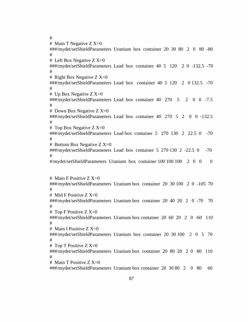
87

#

# Main T Negative Z X=0


#

# Left Box Negative Z X=0

###/mydet/setShieldParameters Lead box container 40 5 120 2 0 -132.5 -70

#

# Right Box Negative Z X=0

###/mydet/setShieldParameters Lead box container 40 5 120 2 0 132.5 -70

#

# Up Box Negative Z X=0

###/mydet/setShieldParameters Lead box container 40 270 5 2 0 0 -7.5

#

# Down Box Negative Z X=0


#

# Top Box Negative Z X=0

###/mydet/setShieldParameters Lead box container 5 270 130 2 22.5 0 -70

#

# Bottom Box Negative Z X=0

###/mydet/setShieldParameters Lead box container 5 270 130 2 -22.5 0 -70

#

#/mydet/setShieldParameters Uranium box container 100 100 100 2 0 0 0

# Main F Positive Z X=0

###/mydet/setShieldParameters Uranium box container 20 30 100 2 0 -105 70

#

# Mid F Positive Z X=0


#

# Top F Positive Z X=0


#

# Main I Positive Z X=0

###/mydet/setShieldParameters Uranium box container 20 30 100 2 0 5 70

#

# Top T Positive Z X=0


#

# Main T Positive Z X=0


88

#

# Left Box Positive Z X=0

###/mydet/setShieldParameters Lead box container 40 5.00 120 2 0 -132.5 70

#

# Right Box Positive Z X=0

###/mydet/setShieldParameters Lead box container 40 5.00 120 2 0 132.5 70

#

# Up Box Positive Z X=0

###/mydet/setShieldParameters Lead box container 40 270 5 2 0 0 132.5

#

# Down Box Positive Z X=0


#

# Top Box Positive Z X=0

###/mydet/setShieldParameters Lead box container 5 270 130 2 22.5 0 70

#

# Bottom Box Positive Z X=0

###/mydet/setShieldParameters Lead box container 5 270 130 2 -22.5 0 70

#


# Main F Negative Z X=-110

/mydet/setShieldParameters Uranium box container 20 30 100 2 -110 -105 -70

#

# Mid F Negative Z X=-110


#

# Top F Negative Z X=-110


#

# Main I Negative Z X=-110

/mydet/setShieldParameters Uranium box container 20 30 100 2 -110 5 -70

#

# Top T Negative Z X=-110


#

# Main T Negative Z X=-110


#

# Left Box Negative Z X=-110

/mydet/setShieldParameters Lead box container 40 5.00 120 2 -110 -132.5 -70

89

#

# Right Box Negative Z X=-110

/mydet/setShieldParameters Lead box container 40 5.00 120 2 -110 132.5 -70

#

# Up Box Negative Z X=-110

/mydet/setShieldParameters Lead box container 40 270 5 2 -110 0 -7.5

#

# Down Box Negative Z X=-110

/mydet/setShieldParameters Lead box container 40 270 5 2 -110 0 -132.5

#

# Top Box Negative Z X=-110

/mydet/setShieldParameters Lead box container 5 270 130 2 -87.5 0 -70

#

# Bottom Box Negative Z X=-110

/mydet/setShieldParameters Lead box container 5 270 130 2 -132.5 0 -70

#


# Main F Positive Z X=-110

/mydet/setShieldParameters Uranium box container 20 30 100 2 -110 -105 70

#

# Mid F Positive Z X=-110


#

# Top F Positive Z X=-110


#

# Main I Positive Z X=-110

/mydet/setShieldParameters Uranium box container 20 30 100 2 -110 5 70

#

# Top T Positive Z X=-110


#

# Main T Positive Z X=-110


#

# Left Box Positive Z X=-110

/mydet/setShieldParameters Lead box container 40 5.00 120 2 -110 -132.5 70

#

# Right Box Positive Z X=-110

/mydet/setShieldParameters Lead box container 40 5.00 120 2 -110 132.5 70

90

#

# Up Box Positive Z X=-110

/mydet/setShieldParameters Lead box container 40 270 5 2 -110 0 132.5

#

# Down Box Positive Z X=-110

/mydet/setShieldParameters Lead box container 40 270 5 2 -110 0 7.5

#

# Top Box Positive Z X=-110

/mydet/setShieldParameters Lead box container 5 270 130 2 -87.5 0 70

#

# Bottom Box Positive Z X=-110

/mydet/setShieldParameters Lead box container 5 270 130 2 -132.5 0 70

#


# Main F Negative Z X=110


#

# Mid F Negative Z X=110


#

# Top F Negative Z X=110


#

# Main I Negative Z X=110


#

# Top T Negative Z X=110


#

# Main T Negative Z X=110


#

# Left Box Negative Z X=110

###/mydet/setShieldParameters Lead box container 40 5.00 120 2 110 -132.5 -70

#

# Right Box Negative Z X=110

###/mydet/setShieldParameters Lead box container 40 5.00 120 2 110 132.5 -70

#

# Up Box Negative Z X=110


91

#

# Down Box Negative Z X=110


#

# Top Box Negative Z X=110


#

# Bottom Box Negative Z X=110


#


# Main F Positive Z X=110


#

# Mid F Positive Z X=110


#

# Top F Positive Z X=110


#

# Main I Positive Z X=110


#

# Top T Positive Z X=110


#

# Main T Positive Z X=110


#

# Left Box Positive Z X=110

###/mydet/setShieldParameters Lead box container 40 5.00 120 2 110 -132.5 70

#

# Right Box Positive Z X=110

###/mydet/setShieldParameters Lead box container 40 5.00 120 2 110 132.5 70

#

# Up Box Positive Z X=110


#

# Down Box Positive Z X=110


92

#

# Top Box Positive Z X=110


#

# Bottom Box Positive Z X=110


#


/mydet/update

#/run/beamOn 14400000

/run/beamOn 30

93

# Configuration file for all scenarios with uranium and lead boxes in the xz


# example, elements are uncommented to run the xz scenario in which

# uranium is unshielded in the positive z region and shielded in the negative z

# region at y = 0 mm. To run another xz scenario, simply comment out the

# elements located at y = 0 and uncomment the desired elements. In the

# Platform and Target section, lines starting with ### can be uncommented.

# Lines beginning with # are permanent comments, as they describe specific

# elements being acted on.

#

#### Cry Settings

/control/verbose 0

/run/verbose 0

/event/verbose 0

/tracking/verbose 0












#/CRY/input

/CRY/update


/vis/verbose 1

/vis/scene/create

#/vis/open OGLIX



/vis/drawVolume

/vis/viewer/zoom 1.




/vis/scene/add/hits


94


/vis/viewer/flush


















THICK POSITION(XYZ)



#

# Main F Negative Z Y=0


#

# Mid F Negative Z Y=0


#

# Top F Negative Z Y=0


#

# Main I Negative Z Y=0

/mydet/setShieldParameters Uranium box container 30 20 100 2 5 0 -70

#

# Top T Negative Z Y=0


#

# Main T Negative Z Y=0

95


#

# Left Box Negative Z Y=0

/mydet/setShieldParameters Lead box container 5.00 40 120 2 -142.5 0 -70

#

# Right Box Negative Z Y=0

/mydet/setShieldParameters Lead box container 5.00 40 120 2 142.5 0 -70

#

# Up Box Negative Z Y=0

/mydet/setShieldParameters Lead box container 290 40 5 2 0 0 -7.5

#

# Down Box Negative Z Y=0


#

# Top Box Negative Z Y=0

/mydet/setShieldParameters Lead box container 290 5 130 2 0 22.5 -70

#

# Bottom Box Negative Z Y=0

/mydet/setShieldParameters Lead box container 290 5 130 2 0 -22.5 -70

#


# Main F Positive Z Y=0


#

# Mid F Positive Z Y=0


#

# Top F Positive Z Y=0


#

# Main I Positive Z Y=0

/mydet/setShieldParameters Uranium box container 30 20 100 2 5 0 70

#

# Top T Positive Z Y=0


#

# Main T Positive Z Y=0


#

# Left Box Positive Z Y=0

96

###/mydet/setShieldParameters Lead box container 5.00 40 120 2 -142.5 0 70

#

# Right Box Positive Z Y=0

###/mydet/setShieldParameters Lead box container 5.00 40 120 2 142.5 0 70

#

# Up Box Positive Z Y=0


#

# Down Box Positive Z Y=0


#

# Top Box Positive Z Y=0

###/mydet/setShieldParameters Lead box container 290 5 130 2 0 22.5 70

#

# Bottom Box Positive Z Y=0

###/mydet/setShieldParameters Lead box container 290 5 130 2 0 -22.5 70

#


# Main F Negative Z Y=-110

###/mydet/setShieldParameters Uranium box container 30 20 100 2 -115 -110 -70

#

# Mid F Negative Z Y=-110


#

# Top F Negative Z Y=-110


#

# Main I Negative Z Y=-110


#

# Top T Negative Z Y=-110


#

# Main T Negative Z Y=-110


#

# Left Box Negative Z Y=-110

###/mydet/setShieldParameters Lead box container 5.00 40 120 2 -142.5 -110 -70

#

# Right Box Negative Z Y=-110

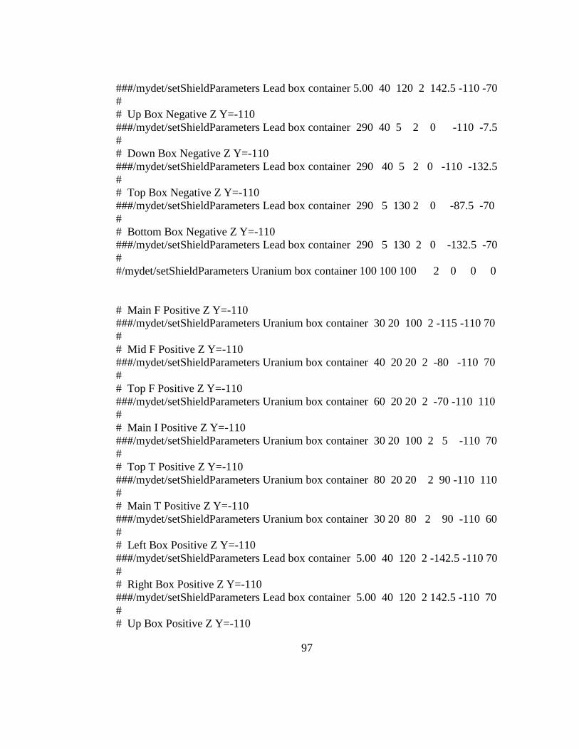
97

###/mydet/setShieldParameters Lead box container 5.00 40 120 2 142.5 -110 -70

#

# Up Box Negative Z Y=-110

###/mydet/setShieldParameters Lead box container 290 40 5 2 0 -110 -7.5

#

# Down Box Negative Z Y=-110


#

# Top Box Negative Z Y=-110


#

# Bottom Box Negative Z Y=-110


#


# Main F Positive Z Y=-110

###/mydet/setShieldParameters Uranium box container 30 20 100 2 -115 -110 70

#

# Mid F Positive Z Y=-110


#

# Top F Positive Z Y=-110


#

# Main I Positive Z Y=-110


#

# Top T Positive Z Y=-110


#

# Main T Positive Z Y=-110


#

# Left Box Positive Z Y=-110

###/mydet/setShieldParameters Lead box container 5.00 40 120 2 -142.5 -110 70

#

# Right Box Positive Z Y=-110

###/mydet/setShieldParameters Lead box container 5.00 40 120 2 142.5 -110 70

#

# Up Box Positive Z Y=-110

98

###/mydet/setShieldParameters Lead box container 290 40 5 2 0 -110 132.5

#

# Down Box Positive Z Y=-110


#

# Top Box Positive Z Y=-110


#

# Bottom Box Positive Z Y=-110


#


# Main F Negative Z Y=110

###/mydet/setShieldParameters Uranium box container 30 20 100 2 -115 110 -70

#

# Mid F Negative Z Y=110


#

# Top F Negative Z Y=110


#

# Main I Negative Z Y=110


#

# Top T Negative Z Y=110


#

# Main T Negative Z Y=110


#

# Left Box Negative Z Y=110

###/mydet/setShieldParameters Lead box container 5.00 40 120 2 -142.5 110 -70

#

# Right Box Negative Z Y=110

###/mydet/setShieldParameters Lead box container 5.00 40 120 2 142.5 110 -70

#

# Up Box Negative Z Y=110


#

# Down Box Negative Z Y=110

99


#

# Top Box Negative Z Y=110


#

# Bottom Box Negative Z Y=110


#


# Main F Positive Z Y=110

###/mydet/setShieldParameters Uranium box container 30 20 100 2 -115 110 70

#

# Mid F Positive Z Y=110


#

# Top F Positive Z Y=110


#

# Main I Positive Z Y=110


#

# Top T Positive Z Y=110


#

# Main T Positive Z Y=110


#

# Left Box Positive Z Y=110


#

# Right Box Positive Z Y=110


#

# Up Box Positive Z Y=110


#

# Down Box Positive Z Y=110


#

# Top Box Positive Z Y=110

100


#

# Bottom Box Positive Z Y=110


#


/mydet/update


/run/beamOn 30

101

# Configuration file for all scenarios with uranium and lead boxes in the xy


# example, elements are uncommented to run scenario xy, z = -110 mm now.

# To run another xy scenario, simply comment out the elements located at z =

# -110 and uncomment the desired elements. In the Platform and Target

# section, lines starting with ### can be uncommented. Lines beginning with #

# are permanent comments, as they describe specific elements being acted on.

#

#### Cry Settings

/control/verbose 0

/run/verbose 0

/event/verbose 0

/tracking/verbose 0












#/CRY/input

/CRY/update


/vis/verbose 1

/vis/scene/create

#/vis/open OGLIX



/vis/drawVolume

/vis/viewer/zoom 1.




/vis/scene/add/hits



/vis/viewer/flush

102


















THICK POSITION(XYZ)



#

# Main F Negative Y Z=0


#

# Mid F Negative Y Z=0


#

# Top F Negative Y Z=0


#

# Main I Negative Y Z=0


#

# Top T Negative Y Z=0


#

# Main T Negative Y Z=0

103


#

# Left Box Negative Y Z=0


#

# Right Box Negative Y Z=0


#

# Up Box Negative Y Z=0


#

# Down Box Negative Y Z=0


#

# Top Box Negative Y Z=0


#

# Bottom Box Negative Y Z=0


#


# Main F Positive Y Z=0


#

# Mid F Positive Y Z=0


#

# Top F Positive Y Z=0


#

# Main I Positive Y Z=0


#

# Top T Positive Y Z=0


#

# Main T Positive Y Z=0


#

# Left Box Positive Y Z=0

104


#

# Right Box Positive Y Z=0


#

# Up Box Positive Y Z=0


#

# Down Box Positive Y Z=0


#

# Top Box Positive Y Z=0


#

# Bottom Box Positive Y Z=0


#


# Main F Negative Y Z=-110


#

# Mid F Negative Y Z=-110


#

# Top F Negative Y Z=-110


#

# Main I Negative Y Z=-110

/mydet/setShieldParameters Uranium box container 30 100 20 2 5 -70 -110

#

# Top T Negative Y Z=-110


#

# Main T Negative Y Z=-110


#

# Left Box Negative Y Z=-110

/mydet/setShieldParameters Lead box container 5.00 120 40 2 -142.5 -70 -110

#

# Right Box Negative Y Z=-110

105

/mydet/setShieldParameters Lead box container 5.00 120 40 2 142.5 -70 -110

#

# Up Box Negative Y Z=-110


#

# Down Box Negative Y Z=-110


#

# Top Box Negative Y Z=-110

/mydet/setShieldParameters Lead box container 290 130 5 2 0 -70 -87.5

#

# Bottom Box Negative Y Z=-110

/mydet/setShieldParameters Lead box container 290 130 5 2 0 -70 -132.5

#


# Main F Positive Y Z=-110


#

# Mid F Positive Y Z=-110


#

# Top F Positive Y Z=-110


#

# Main I Positive Y Z=-110


#

# Top T Positive Y Z=-110


#

# Main T Positive Y Z=-110


#

# Left Box Positive Y Z=-110

/mydet/setShieldParameters Lead box container 5.00 120 40 2 -142.5 70 -110

#

# Right Box Positive Y Z=-110

/mydet/setShieldParameters Lead box container 5.00 120 40 2 142.5 70 -110

#

# Up Box Positive Y Z=-110

106


#

# Down Box Positive Y Z=-110


#

# Top Box Positive Y Z=-110


#

# Bottom Box Positive Y Z=-110


#


# Main F Negative Y Z=110


#

# Mid F Negative Y Z=110


#

# Top F Negative Y Z=110


#

# Main I Negative Y Z=110


#

# Top T Negative Y Z=110


#

# Main T Negative Y Z=110


#

# Left Box Negative Y Z=110


#

# Right Box Negative Y Z=110


#

# Up Box Negative Y Z=110


#

# Down Box Negative Y Z=110

107


#

# Top Box Negative Y Z=110


#

# Bottom Box Negative Y Z=110


#


# Main F Positive Y Z=110


#

# Mid F Positive Y Z=110


#

# Top F Positive Y Z=110


#

# Main I Positive Y Z=110


#

# Top T Positive Y Z=110


#

# Main T Positive Y Z=110


#

# Left Box Positive Y Z=110


#

# Right Box Positive Y Z=110


#

# Up Box Positive Y Z=110


#

# Down Box Positive Y Z=110


#

# Top Box Positive Y Z=110

108


#

# Bottom Box Positive Y Z=110


#


/mydet/update


/run/beamOn 30

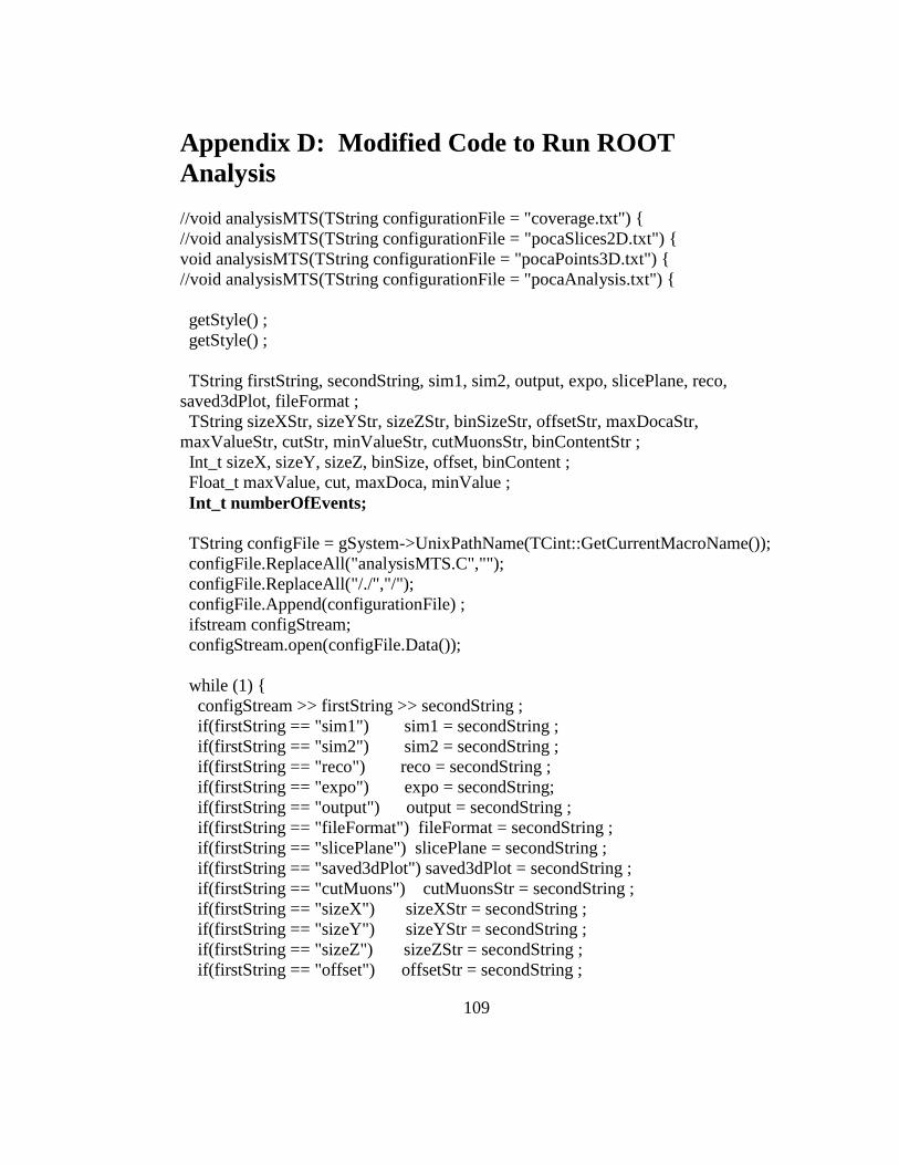
109

Appendix D: Modified Code to Run ROOT

Analysis

//void analysisMTS(TString configurationFile = "coverage.txt") {

//void analysisMTS(TString configurationFile = "pocaSlices2D.txt") {

void analysisMTS(TString configurationFile = "pocaPoints3D.txt") {

//void analysisMTS(TString configurationFile = "pocaAnalysis.txt") {

getStyle() ;

getStyle() ;

TString firstString, secondString, sim1, sim2, output, expo, slicePlane, reco,

saved3dPlot, fileFormat ;

TString sizeXStr, sizeYStr, sizeZStr, binSizeStr, offsetStr, maxDocaStr,

maxValueStr, cutStr, minValueStr, cutMuonsStr, binContentStr ;

Int_t sizeX, sizeY, sizeZ, binSize, offset, binContent ;

Float_t maxValue, cut, maxDoca, minValue ;

Int_t numberOfEvents;

TString configFile = gSystem->UnixPathName(TCint::GetCurrentMacroName());

configFile.ReplaceAll("analysisMTS.C","");

configFile.ReplaceAll("/./","/");

configFile.Append(configurationFile) ;

ifstream configStream;

configStream.open(configFile.Data());

while (1) {

configStream >> firstString >> secondString ;

if(firstString == "sim1") sim1 = secondString ;

if(firstString == "sim2") sim2 = secondString ;

if(firstString == "reco") reco = secondString ;

if(firstString == "expo") expo = secondString;

if(firstString == "output") output = secondString ;

if(firstString == "fileFormat") fileFormat = secondString ;

if(firstString == "slicePlane") slicePlane = secondString ;

if(firstString == "saved3dPlot") saved3dPlot = secondString ;

if(firstString == "cutMuons") cutMuonsStr = secondString ;

if(firstString == "sizeX") sizeXStr = secondString ;

if(firstString == "sizeY") sizeYStr = secondString ;

if(firstString == "sizeZ") sizeZStr = secondString ;

if(firstString == "offset") offsetStr = secondString ;

110

if(firstString == "binSize") binSizeStr = secondString ;

if(firstString == "maxDoca") maxDocaStr = secondString ;

if(firstString == "maxValue") maxValueStr = secondString ;

if(firstString == "cut") cutStr = secondString ;

if(firstString == "minValue") minValueStr = secondString ;

if(firstString == "binContent") binContentStr = secondString ;

if(firstString == "numberOfEvents") numberOfEvents = atoi

(secondString.Data());

if (!configStream.good()) break ;

}

sizeX = atoi(sizeXStr.Data()) ;

sizeY = atoi(sizeYStr.Data()) ;

sizeZ = atoi(sizeZStr.Data()) ;

offset = atoi(offsetStr.Data()) ;

binSize = atoi(binSizeStr.Data()) ;

cutMuons = atoi(cutMuonsStr.Data()) ;

cut = atof(cutStr.Data()) ;

maxDoca = atof(maxDocaStr.Data()) ;

maxValue = atof(maxValueStr.Data()) ;

minValue = atof(minValueStr.Data()) ;

binContent = atoi(binContentStr.Data()) ;

printf("sim1 %s\n",sim1.Data());

printf("sim2 %s\n",sim2.Data());

printf("reco %s\n",reco.Data());

printf("expo %s\n",expo.Data());

printf("output %s\n",output.Data());

printf("fileFormat %s\n",fileFormat.Data());

printf("slicePlane %s\n",slicePlane.Data());

printf("saved3dPlot %s\n",saved3dPlot.Data());

printf("cutMuons %d\n",cutMuons);

printf("sizeX %d\n",sizeX);

printf("sizeY %d\n",sizeY);

printf("sizeZ %d\n",sizeZ);

printf("binContent %d\n",binContent);

printf("offset %d\n",offset);

printf("binSize %d\n",binSize);

printf("cut %f\n",cut);

printf("maxDoca %f\n",maxDoca);

printf("maxValue %f\n",maxValue);

printf("minValue %f\n",minValue);

111

TFile *f = new TFile(Form("%s.root",sim1.Data()),"RECREATE");

Int_t nbinx = sizeX/binSize;

Int_t nbiny = sizeY/binSize;

Int_t nbinz = sizeZ/binSize;

Int_t total1, total2 ;

Float_t norm = 1 ;

Int_t maximum = maxValue ;

if(output == "pocaAnalysis") {

getPocaRecoAnalysis(sim1,output,reco,fileFormat,sizeX,sizeY,sizeZ,binSize) ;

getPocaRecoAnalysis(sim2,output,reco,fileFormat,sizeX,sizeY,sizeZ,binSize) ;

}

if(output == "coverage3d") {

if (output == "coverage3d") maximum = getCoverageMax(sim1,sim2) ;

get3dPlots(sim1,expo,output,reco,fileFormat,maximum,cut,0,sizeX,sizeY,sizeZ,bin

Size,cutMuons,binContent,saved3dPlot) ;

get3dPlots(sim2,expo,output,reco,fileFormat,maximum,cut,0,sizeX,sizeY,sizeZ,bin

Size,cutMuons,binContent,saved3dPlot) ;

}

if(output == "pocaPoints3d") {

total1 = getExpoTime(sim1,expo,output,fileFormat) ;

total2 = getExpoTime(sim2,expo,output,fileFormat) ;

get3dPlots(sim1,expo,output,reco,fileFormat,maximum,cut,total1,sizeX,sizeY,size

Z,binSize,cutMuons,binContent,saved3dPlot,numberOfEvents) ;

get3dPlots(sim2,expo,output,reco,fileFormat,maximum,cut,total1,sizeX,sizeY,size

Z,binSize,cutMuons,binContent,saved3dPlot,numberOfEvents) ;

}


norm = getCoverageMax(sim1,sim2) ;

printf(" max= %d\n",maximum);

get2DSlicedHists(sim1,sim2,slicePlane,expo,output,reco,fileFormat,0,0,norm,size

X,sizeY,sizeZ,binSize,offset,maxValue,cut,minValue,cutMuons) ;

}

112

if(output == "poca2dSlices"){

get2DSlicedHists(sim1,sim2,slicePlane,expo,output,reco,fileFormat,total1,total2,no

rm,sizeX,sizeY,sizeZ,binSize,offset,maxValue,cut,minValue,cutMuons) ;

}

configStream.close() ;

f->Write();

}

void getStyle() {

gROOT->Reset();

gStyle->SetOptStat(0);

gStyle->SetCanvasColor(0) ;

gStyle->SetCanvasBorderMode(0) ;

gStyle->SetLabelFont(62,"xyz");

gStyle->SetLabelSize(0.03,"xyz");

gStyle->SetLabelColor(1,"xyz");

gStyle->SetTitleBorderSize(0) ;

gStyle->SetTitleFillColor(0) ;

gStyle->SetTitleSize(0.075,"xyz");

gStyle->SetTitleOffset(4.5,"xyz");

gStyle->SetPalette(1);

const Int_t NRGBs = 5;

const Int_t NCont = 255;

Double_t stops[NRGBs] = { 0.00, 0.34, 0.61, 0.84, 1.00 };

Double_t red[NRGBs] = { 0.00, 0.00, 0.87, 1.00, 0.51 };

Double_t green[NRGBs] = { 0.00, 0.81, 1.00, 0.20, 0.00 };

Double_t blue[NRGBs] = { 0.51, 1.00, 0.12, 0.00, 0.00 };

TColor::CreateGradientColorTable(NRGBs, stops, red, green, blue, NCont);

gStyle->SetNumberContours(NCont);

}

Int_t getExpoTime(TString sim, TString expo, TString output, TString fileFormat)

{

TString dir = gSystem->UnixPathName(TCint::GetCurrentMacroName());

dir.ReplaceAll("analysisMTS.C","");

dir.ReplaceAll("/./","/");

dir.Append(sim) ;

113

ifstream in;

in.open(Form("%s.txt",dir.Data()));

Float_t x, y, z, meanAngle, lambda, doca;

Int_t nTotal = 0;

while (1) {

if(fileFormat == "angle") in >> x >> y >> z >> meanAngle ;

if(fileFormat == "angleLambda") in >> x >> y >> z >> meanAngle >> lambda

;

if(fileFormat == "angleLambdaDoca") in >> x >> y >> z >> meanAngle >>

lambda >> doca ;

if (!in.good()) break ;

nTotal++ ;

}

if(expo == "4Min") nTotal = (Int_t) (nTotal/2.5) ;

if(expo == "1Min") nTotal = (Int_t) (nTotal/10) ;

printf("%d muons in the MTS for %s exposure time\n",nTotal,expo.Data());

in.close() ;

return nTotal ;

}

Int_t getCoverageMax(TString sim1, TString sim2) {

TString dir1 = gSystem->UnixPathName(TCint::GetCurrentMacroName());

dir1.ReplaceAll("analysisMTS.C","");

dir1.ReplaceAll("/./","/");

dir1.Append(sim1) ;

ifstream in1;

in1.open(Form("%s.txt",dir1.Data()));




dir2.Append(sim2) ;

ifstream in2;


Float_t x, y, z ;

Int_t nlines, coverage, max1, max2, max ;

114

while (1) {

in1 >> x >> y >> z >> coverage ;

if (!in1.good()) break ;

if (coverage > max1) max1 = coverage ;

nlines++ ;

}

printf(" found %d points, max1 value: %d\n",nlines,max1) ;

in1.close() ;

nlines = 0 ;

while (1) {

in2 >> x >> y >> z >> coverage ;

if (!in2.good()) break ;

if (coverage > max2) max2 = coverage ;

nlines++ ;

}

printf(" found %d points, max2 value: %d\n",nlines,max2) ;

in2.close() ;

nlines = 0 ;

if (max1>max2) max = max1 ;

else max = max2 ;

return max ;

}

void getPocaRecoAnalysis(TString sim, TString output, TString reco, TString

fileFormat, Int_t sizeX, Int_t sizeY, Int_t sizeZ, Int_t binSize){




dir.Append(sim) ;

ifstream in;


Int_t nbinx = sizeX/binSize ;

Int_t nbiny = sizeY/binSize ;

Int_t nbinz = sizeZ/binSize ;

Float_t x, y, z, meanAngle, lambda, parameter, doca, docaReco;

Int_t nlines, coverage;

115

// h3d = new TH3F("3dPoca","3dPoca", nbinx,-sizeX/2,sizeX/2,nbiny,-

sizeY/2,sizeY/2,nbinz,-sizeZ/2,sizeZ/2);

h1d = new TH1F("1dPoca","1dPoca", nbinx,-sizeX/2,sizeX/2);

h1dNorm = new TH1F("1dPocaNorm","1dPocaNorm", nbinx,-sizeX/2,sizeX/2);

while (1) {

if(fileFormat == "coverage") in >> x >> y >> z >> coverage ;



;


lambda >> doca ;

if (!in.good()) break;

if((x>=-sizeX/2) && (x<=sizeX/2) && (y>=-sizeY/2) && (y<=sizeY/2) &&

(z>=-sizeZ/2) && (z<=sizeZ/2)) {

if(fileFormat == "coverage") parameter = coverage ;

if(fileFormat == "angle") parameter = meanAngle ;

if((fileFormat == "angleLambda") && (reco == "lambda")) parameter =

lambda ;

if((fileFormat == "angleLambda") && (reco == "meanAngle")) parameter =

meanAngleileFormat angleLambdaDoca

;

if((fileFormat == "angleLambdaDoca") && (reco == "doca")) parameter =

doca ;

if((fileFormat == "angleLambdaDoca") && (reco == "lambda")) parameter =

lambda ;

if((fileFormat == "angleLambdaDoca") && (reco == "meanAngle")) parameter

= meanAngle ;

if((fileFormat == "angleLambdaDoca") && (reco == "docaReco")) parameter

= lambda/doca ;

h1d->Fill(x,parameter) ;

h1dNorm->Fill(x) ;

nlines++ ;

}

}

h1d->Divide(h1dNorm) ;

}

void get3dPlots(TString sim, TString expo, TString output, TString reco, TString

fileFormat, Float_t maxValue, Float_t cut, Int_t total, Int_t sizeX, Int_t sizeY, Int_t

116

sizeZ, Int_t binSize, Int_t nbMuonCut, Int_t binContent, TString saved3dPlot, Int_t

numberOfEvents) {




dir.Append(sim) ;

ifstream in;


dir.ReplaceAll("10Min",expo.Data());

Int_t nbinx = sizeX/binSize ;

Int_t nbiny = sizeY/binSize ;

Int_t nbinz = sizeZ/binSize ;

Float_t x, y, z, meanAngle, lambda, parameter, doca, docaReco;

Int_t nlines, coverage;

TNtuple *ntuple = new TNtuple(Form("ntuple %s",sim.Data()),"data from ascii

file","x:y:z:parameter");

Int_t numberOfEventsCounter = 0;

while (1) {

if(fileFormat == "coverage") in >> x >> y >> z >> coverage ;



;


lambda >> doca ;

if (!in.good() || numberOfEventsCounter >= numberOfEvents) break;

numberOfEventsCounter++;

if((x>=-sizeX/2) && (x<=sizeX/2) && (y>=-sizeY/2) && (y<=sizeY/2) &&

(z>=-sizeZ/2) && (z<=sizeZ/2)) {




lambda ;


meanAngle ;

117


doca ;


lambda ;


= meanAngle ;

if((fileFormat == "angleLambdaDoca") && (reco == "docaReco")) parameter

= lambda/doca ;

if(output != "coverage3d") {

if(parameter > cut) {

if(parameter > maxValue) parameter = maxValue ;

ntuple->Fill(x,y,z,parameter) ;

}

}

Float_t xMean = 0.0 ;

Float_t yMean = 0.0 ;

Float_t zMean = 0.0 ;

Int_t ii = 0 ;

Int_t jj = 0 ;

Int_t kk = 0 ;

Int_t increment = Int_t (binSize/binContent) ;


for(ii=0; ii<binContent; ii++) {

for(jj=0; jj<binContent; jj++) {

for(kk=0; kk<binContent; kk++) {

xMean = x -0.5*binSize + ii*increment ;

yMean = y -0.5*binSize + jj*increment ;

zMean = z -0.5*binSize + kk*increment ;

ntuple->Fill(xMean,yMean,zMean,parameter) ;

}

}

}

}

nlines++ ;

if(nlines == total) break ;

}

}

printf(" found %d points for histograms\n",nlines);

118

if((output == "pocaPoints3d") || (output == "coverage3d")) {

ntuple->Fill(-sizeX/2,-sizeY/2,-sizeZ/2,maxValue) ;

ntuple->Fill(-sizeX/2,-sizeY/2,sizeZ/2,maxValue) ;

ntuple->Fill(-sizeX/2,sizeY/2,-sizeZ/2,maxValue) ;

ntuple->Fill(-sizeX/2,sizeY/2,sizeZ/2,maxValue) ;

ntuple->Fill(sizeX/2,-sizeY/2,-sizeZ/2,maxValue) ;

ntuple->Fill(sizeX/2,-sizeY/2,sizeZ/2,maxValue) ;

ntuple->Fill(sizeX/2,sizeY/2,-sizeZ/2,maxValue) ;

ntuple->Fill(sizeX/2,sizeY/2,sizeZ/2,maxValue) ;

if(reco == "doca") ntuple->SetTitle("3d poca-doca");

if(reco == "lambda") ntuple->SetTitle("3d poca-lambda");

if(reco == "meanAngle") ntuple->SetTitle("3d poca-meanAngle");

if(reco == "coverage3d") ntuple->SetTitle("3d coverage");

if(saved3dPlot == "yes") {

TString pictureName = image3DFileName(sim, output, cut, maxValue,

"3D.png") ;

TCanvas c("3D plots","3D em-plots",80,80,1000,600);

c.cd();

ntuple->Draw("z:y:x:parameter","","colz") ;

ntuple->UseCurrentStyle();

c.SaveAs(pictureName);

}

else {

ntuple->Draw("z:y:x:parameter","","colz") ;

ntuple->UseCurrentStyle();

}

}

in.close();

}

void get2DSlicedHists(TString sim1,TString sim2,TString slicePlane,TString

expo,TString output,TString reco,TString fileFormat,Int_t total1,Int_t total2,Int_t

norm,Int_t sizeX,Int_t sizeY,Int_t sizeZ,Float_t binSize,Int_t offset,Float_t

maxValue,Float_t cut,Float_t minValue,Int_t nbMuonCut) {


119



dir1.Append(sim1) ;




dir2.Append(sim2) ;

ifstream in1, in2;



dir1.ReplaceAll("10Min",expo.Data());

dir2.ReplaceAll("10Min",expo.Data());

Int_t size1 = sizeX ;

Int_t size2 = sizeY ;

Int_t size3 = sizeZ ;

Int_t nbin1 = sizeX/binSize ;

Int_t nbin2 = sizeY/binSize ;

Int_t nbin3 = sizeZ/binSize ;

TString histTitle1 = "h1xy2d" ;

TString histTitle2 = "h2xy2d" ;

if(slicePlane == "XZ") {

nbin1 = sizeX/binSize ;

nbin2 = sizeZ/binSize ;

nbin3 = sizeY/binSize ;

size1 = sizeX ;

size2 = sizeZ ;

size3 = sizeY ;

histTitle1 = "h1xz2d" ;

histTitle2 = "h2xz2d" ;

}

if(slicePlane == "YZ") {

nbin1 = sizeY/binSize ;

nbin2 = sizeZ/binSize ;

120

nbin3 = sizeX/binSize ;

size1 = sizeY ;

size2 = sizeZ ;

size3 = sizeX ;

histTitle1 = "h1yz2d" ;

histTitle2 = "h2yz2d" ;

}

Float_t x, y, z, coverage, meanAngle, lambda, doca, parameter;

Int_t nlines = 0;

TH2F *h2d1[200];

TH2F *h2d1N[200];

TH2F *h2d2[200];

TH2F *h2d2N[200];

TH2F *h2dratio[200];

TH2F *hdoca1[200];

TH2F *hdoca2[200];

for(int k=0; k<200; k++) {

TString title2d1Hist = histTitle1.Append(sim1) ;

TString title2d2Hist = histTitle2.Append(sim2) ;

h2d1[k] = new

TH2F(title2d1Hist.Append(Form("%d",k)),title2d1Hist.Append(Form("%d",k)),

nbin1,-size1/2,size1/2,nbin2,-size2/2,size2/2);

h2d1N[k] = new TH2F(Form("1%d",k),Form("1%d",k), nbin1,-

size1/2,size1/2,nbin2,-size2/2,size2/2);

h2d2[k] = new

TH2F(title2d2Hist.Append(Form("%d",k)),title2d2Hist.Append(Form("%d",k)),

nbin1,-size1/2,size1/2,nbin2,-size2/2,size2/2);

h2d2N[k] = new TH2F(Form("2%d",k),Form("2%d",k), nbin1,-

size1/2,size1/2,nbin2,-size2/2,size2/2);

hdoca1[k] = new

TH2F(title2d1Hist.Append(Form("doca1%d",k)),title2d1Hist.Append(Form("doca

1%d",k)),nbin1,-size1/2,size1/2,nbin2,-size2/2,size2/2);

121

hdoca2[k] = new

TH2F(title2d1Hist.Append(Form("doca2%d",k)),title2d1Hist.Append(Form("doca

2%d",k)),nbin1,-size1/2,size1/2,nbin2,-size2/2,size2/2);

if(output =="coverage2d") h2dratio[k] = new TH2F(Form("ratio

%d",k),Form("ratio %d",k), nbin1,-size1/2,size1/2,nbin2,-size2/2,size2/2);

}

while (1) {

if(fileFormat == "coverage") in1 >> x >> y >> z >> coverage ;

if(fileFormat == "angle") in1 >> x >> y >> z >> meanAngle ;

if(fileFormat == "angleLambda") in1 >> x >> y >> z >> meanAngle >>

lambda ;

if(fileFormat == "angleLambdaDoca") in1 >> x >> y >> z >> meanAngle >>

lambda >> doca ;

if (!in1.good()) break;




lambda ;


meanAngle ;


doca ;


lambda ;


= meanAngle ;

if((fileFormat == "angleLambdaDoca") && (reco == "docaReco")) parameter =

lambda/doca ;

if(slicePlane == "XY") {

if((x>=-sizeX/2)&&(x<=sizeX/2)&&(y>=-

sizeY/2)&&(y<=sizeY/2)&&(z>=(offset-sizeZ/2))&&(z<=(offset+sizeZ/2))) {

Int_t j = (Int_t) ((size3/2 + offset - z)/binSize) + 1 ;

Int_t k = nbin3 - j ;

if(k<0) k=0 ;

h2d1[k]->Fill(x,y,parameter) ;

hdoca1[k]->Fill(x,y,doca) ;

h2d1N[k]->Fill(x,y) ;

if(output =="coverage2d") h2dratio[k]->Fill(x,y,parameter) ;

}

}

122


if((x>=-sizeX/2)&&(x<=sizeX/2)&&(y>=(offset-

sizeY/2))&&(y<=(offset+sizeY/2))&&(z>=-sizeZ/2)&&(z<=sizeZ/2)) {

Int_t j = (Int_t) ((size3/2 + offset - y)/binSize) + 1 ;


if(k<0) k=0 ;

h2d1[k]->Fill(x,z,parameter) ;

hdoca1[k]->Fill(x,z,doca) ;

h2d1N[k]->Fill(x,z) ;

if(output =="coverage2d") h2dratio[k]->Fill(x,z,parameter) ;

}

}


if((x>=(offset-sizeX/2))&&(x<=(offset+sizeX/2))&&(y>=-

sizeY/2)&&(y<=sizeY/2)&&(z>=-sizeZ/2)&&(z<=sizeZ/2)) {

Int_t j = (Int_t) ((size3/2 + offset - x)/binSize) + 1 ;


if(k<0) k=0 ;

h2d1[k]->Fill(y,z,parameter) ;


h2d1N[k]->Fill(y,z) ;

if(output =="coverage2d") h2dratio[k]->Fill(y,z,parameter) ;

}

}

nlines++;

if(nlines == total1) break ;

}

nlines = 0 ;

while (1) {

if(fileFormat == "coverage") in2 >> x >> y >> z >> coverage ;

if(fileFormat == "angle") in2 >> x >> y >> z >> meanAngle ;

if(fileFormat == "angleLambda") in2 >> x >> y >> z >> meanAngle >>

lambda ;

if(fileFormat == "angleLambdaDoca") in2 >> x >> y >> z >> meanAngle >>

lambda >> doca ;

if (!in2.good()) break;



123


lambda ;


meanAngle ;


doca ;


lambda ;


= meanAngle ;

if((fileFormat == "angleLambdaDoca") && (reco == "docaReco")) parameter =

lambda/doca ;


if((x>=-sizeX/2)&&(x<=sizeX/2)&&(y>=-

sizeY/2)&&(y<=sizeY/2)&&(z>=(offset-sizeZ/2))&&(z<=(offset+sizeZ/2))) {

Int_t j = (Int_t) ((size3/2 + offset - z)/binSize) + 1 ;


if(k<0) k=0 ;

h2d2[k]->Fill(x,y,parameter) ;


h2d2N[k]->Fill(x,y) ;

}

}


if((x>=-sizeX/2)&&(x<=sizeX/2)&&(y>=(offset-

sizeY/2))&&(y<=(offset+sizeY/2))&&(z>=-sizeZ/2)&&(z<=sizeZ/2)) {

Int_t j = (Int_t) ((size3/2 + offset - y)/binSize) + 1 ;


if(k<0) k=0 ;

h2d2[k]->Fill(x,z,parameter) ;

hdoca2[k]->Fill(x,z,doca) ;

h2d2N[k]->Fill(x,z) ;

}

}


if((x>=(offset-sizeX/2))&&(x<=(offset+sizeX/2))&&(y>=-

sizeY/2)&&(y<=sizeY/2)&&(z>=-sizeZ/2)&&(z<=sizeZ/2)) {

Int_t j = (Int_t) ((size3/2 + offset - x)/binSize) + 1 ;


if(k<0) k=0 ;

124

h2d2[k]->Fill(y,z,parameter) ;

hdoca2[k]->Fill(y,z,doca) ;

h2d2N[k]->Fill(y,z) ;

}

}

nlines++;

if(nlines == total2) break ;

}

for(int k=0; k<nbin3; k++) {

Int_t voxel = -size3/2 + offset + (k+0.5)*binSize ;

Float_t maxVal = 1.0 ;


maxVal = 1 ;

h2dratio[k]->Divide(h2d2[k]) ;

save2dSlicedHists(h2d1[k],sim1,slicePlane,output,"",norm,voxel,k,maxVal,minVal

ue) ;

save2dSlicedHists(h2d2[k],sim2,slicePlane,output,"",norm,voxel,k,maxVal,minVal

ue) ;

save2dSlicedHists(h2dratio[k],"ratio",slicePlane,output,"",1,voxel,k,2,0) ;

}

else {

maxVal = maxValue ;

if(reco == "docaReco") {

h2d1[k]->Divide(hdoca1[k]) ;

h2d2[k]->Divide(hdoca2[k]) ;

}

else {

h2d1[k]->Divide(h2d1N[k]) ;

h2d2[k]->Divide(h2d2N[k]) ;

}

for(int i=0; i<nbin1; i++) {

for(int j=0; j<nbin2; j++) {

Int_t nbMuons1 = h2d1N[k]->GetBinContent(i,j) ;

Int_t nbMuons2 = h2d2N[k]->GetBinContent(i,j) ;

Float_t param1 = h2d1[k]->GetBinContent(i,j) ;

Float_t param2 = h2d2[k]->GetBinContent(i,j) ;

125

if((nbMuons1 < nbMuonCut) || (param1 < cut)) {

h2d1[k]->SetBinContent(i,j,0) ;

h2d1N[k]->SetBinContent(i,j,0) ;

}

if((nbMuons2 < nbMuonCut) || (param1 < cut)) {

h2d2[k]->SetBinContent(i,j,0) ;

h2d2N[k]->SetBinContent(i,j,0) ;

}

}

}

save2dSlicedHists(h2d1[k],sim1,slicePlane,output,reco,norm,voxel,k,maxVal,min

Value) ;

save2dSlicedHists(h2d2[k],sim2,slicePlane,output,reco,norm,voxel,k,maxVal,min

Value) ;

}

}

in1.close();

in2.close();

}

void save2dSlicedHists(TH2F *h2d, TString input, TString slicePlane, TString

output, TString reco, Float_t norm, Int_t sliceCut, Int_t number, Float_t maxVal,

Float_t minVal) {

TString title =

image2DFileName(input,reco,slicePlane,norm,sliceCut,number,"") ;

TString pictureName =

image2DFileName(input,reco,slicePlane,0.0,sliceCut,number,".png") ;


h2d->Scale(1/norm) ;

h2d->Smooth();

}


h2d->GetXaxis()->SetTitle("X [mm]");

h2d->GetYaxis()->SetTitle("Y [mm]");

}

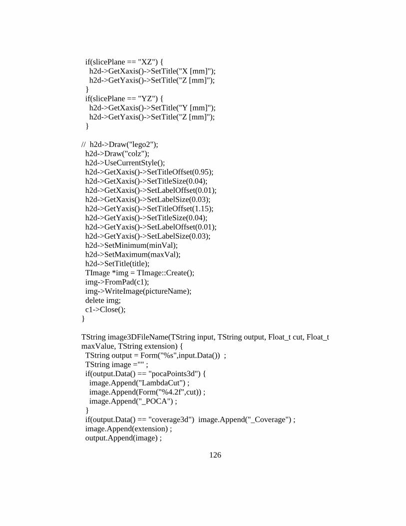
126


h2d->GetXaxis()->SetTitle("X [mm]");

h2d->GetYaxis()->SetTitle("Z [mm]");

}


h2d->GetXaxis()->SetTitle("Y [mm]");

h2d->GetYaxis()->SetTitle("Z [mm]");

}

// h2d->Draw("lego2");

h2d->Draw("colz");

h2d->UseCurrentStyle();

h2d->GetXaxis()->SetTitleOffset(0.95);

h2d->GetXaxis()->SetTitleSize(0.04);

h2d->GetXaxis()->SetLabelOffset(0.01);

h2d->GetXaxis()->SetLabelSize(0.03);

h2d->GetYaxis()->SetTitleOffset(1.15);

h2d->GetYaxis()->SetTitleSize(0.04);

h2d->GetYaxis()->SetLabelOffset(0.01);

h2d->GetYaxis()->SetLabelSize(0.03);

h2d->SetMinimum(minVal);

h2d->SetMaximum(maxVal);

h2d->SetTitle(title);

TImage *img = TImage::Create();

img->FromPad(c1);

img->WriteImage(pictureName);

delete img;

c1->Close();

}

TString image3DFileName(TString input, TString output, Float_t cut, Float_t

maxValue, TString extension) {

TString output = Form("%s",input.Data()) ;

TString image ="" ;

if(output.Data() == "pocaPoints3d") {

image.Append("LambdaCut") ;

image.Append(Form("%4.2f",cut)) ;

image.Append("_POCA") ;

}

if(output.Data() == "coverage3d") image.Append("_Coverage") ;

image.Append(extension) ;

output.Append(image) ;

127

return output ;

}

TString image2DFileName(TString input, TString reco, TString slicePlane, Float_t

norm, Int_t sliceCut, Int_t number, TString extension) {

TString sliceAxis ;

if(slicePlane == "XY") sliceAxis ="Z" ;

if(slicePlane == "XZ") sliceAxis ="Y" ;

if(slicePlane == "YZ") sliceAxis ="X" ;

TString output = Form("%s",input.Data()) ;

TString slicePlane = Form("%sat%s",slicePlane.Data(),sliceAxis.Data()) ;

output.Append(reco) ;

output.Append(slicePlane) ;

output.Append(Form("%d",number)) ;

output.Append("_") ;

TString image ;

image = Form("%d",sliceCut) ;

image.Append("mm") ;

image.ReplaceAll("-","minus") ;

if(norm !=0) {

image.Append("_max") ;

image.Append(Form("%4.0f",norm)) ;

}

image.Append(extension) ;

output.Append(image) ;

return output ;

}

128

Appendix E: Simulated Scenarios Not in Body of

Thesis

The following images are of time exposures of 4 minutes, 10 minutes, and 60

minutes for simulated scenarios mentioned in the body of the thesis. They are

presented here in the order in which they are given in the thesis and begin on the

following page.

Designs for Muon Tomography Station Prototypes Using GEM ... · iv I designed and ran simulations...

Documents

Transcript of Designs for Muon Tomography Station Prototypes Using GEM ... · iv I designed and ran simulations...