1

April 13, 2012 In press Drug Information Journal

Designing Phase 2 Trials Based on Program-Level Considerations:

A Case Study for Neuropathic Pain

Nitin Patel1, James Bolognese1, Christy Chuang-Stein2, David Hewitt3, Arnold Gammaitoni4, Jose Pinheiro5

1Cytel, Inc. 2Pfizer, Inc. 3 Merck and Co., Inc. 4Nuvo Research, Inc. 5Janssen R&D

Abstract

Traditionally, sample size considerations for phase 2 trials are based on the desired properties of the design and response information from the trials. In this paper, we propose to design phase 2 trials based on program-level optimization. We present a framework to evaluate the impact that several phase 2 design features have on the probability of phase 3 success and the expected net present value of the product. These factors include the phase 2 sample size, decision rules to select a dose for phase 3 trials and the sample size for phase 3 trials. Using neuropathic pain as an example, we use simulations to illustrate the framework and show the benefit of including these factors in the overall decision process.

Key Words and Phrases: Maximum utility dose selection method; Net present value; Probability of success; Target efficacy dose selection method.

1. Background Traditionally, product development is divided into distinct phases and planning is carried out for each phase separately. When determining the sample size for a trial, most clinical trialists focus on statistical power or the desired precision in estimation although some researchers have advocated for cost-effective trial designs.1-3 Recently, researchers have paid increasing attention to the concept of assurance (probability of success). They state that the assurance should be at an acceptable level when planning a confirmatory trial.4-7 There is also some published work on examining development strategies beyond a single trial and more quantitative approaches to making go/no go decisions between phases.8-14 These efforts have raised questions of how to optimize study design in the context of a development program and how to choose appropriate criteria for optimization. Concerns over products’ effective patent life have led many product developers to place a premium on speed. A longer remaining patent life at the point of product launch will translate to higher net revenue for the developer. Patel and Ankolekar proposed to incorporate economic factors in deciding sample size and design for clinical trials as well as assessing portfolios of drugs.15 Burman et al used a decision analytic approach to calculate sample size from a perspective of maximizing company profits.9 Mehta and Patel use net revenue and net present value (NPV) as factors when considering sample size re-estimation in a confirmatory trial.16 Similar ideas related to NPV are also part of the assessment criteria.9, 11-12 Despite such efforts, NPV has rarely been formally incorporated into decisions on design strategy. In this paper, we expand the NPV concept in Mehta and Patel16 to designing a phase 2 trial, choosing a dose selection method and planning future phase 3 trials. We investigate how phase 2 design, go/no go

2

decision, dose selection and phase 3 design jointly impact the expected NPV (ENPV). We also examine how these decisions together could affect the probability of success (PoS) of the confirmatory stage. The work reported here is part of a broad industry-academic Adaptive Program subteam of the Adaptive Design Scientific Working Group of the Drug Information Association (formerly under PhRMA) to look at the value of program-level optimization. Our paper is the first report from the Adaptive Program subteam where the program-level considerations are investigated under the conventional product development paradigm, under which both the phase 2 and the phase 3 trials employ fixed designs with no adaptations. Work is ongoing to expand the framework to include both study and program-level adaptations. Even though decision rules within the framework will become more complicated, the basic structure of the framework will remain the same. We illustrate program-level optimization in an effort to obtain an indication for neuropathic pain. According to a survey reported by Torrance et al, the prevalence of pain of predominantly neuropathic origin was about 8%.17 (See additionally, Bouhassira et al.18 ) Neuropathic pain may result from disorders of the peripheral nervous system or the central nervous system (brain and spinal cord). To investigate the strategy for late-stage development of a neuropathic pain medicine, we assume that one phase 2 study is conducted, and the results are used to determine whether phase 3 trials should be launched. If the answer is yes, two identical phase 3 trials will be conducted. We have developed a framework to evaluate the impact of several factors on PoS and the expected NPV. The factors upon which optimization will occur include sample size in phase 2, decision rules to select a dose for phase 3 trials and the sample size for phase 3 trials. We use simulations to illustrate the framework and show how important factors could be incorporated in the overall decision process. In the case study presented in this paper, PoS is defined as the probability that both pivotal phase 3 trials demonstrate a statistically significant drug effect. The expected return is measured by the expected NPV discounted by a factor reflecting the declining monetary value over time. The expected return is affected by effective patent life, trial costs, relationship of efficacy and the tolerability profile of the new product (at the recommended dose), related products already on the market place, and profits of these marketed products. We will illustrate how these factors could be incorporated into the overall assessment.

2. Endpoints to Measure Drug Effect in Neuropathic Pain 2.1 Efficacy The proposed primary measure of efficacy, for the purposes of this exercise, uses the 0-10 numeric rating scale (NRS) based on recent work.19 This scale is popular with clinical researchers, is well validated to detect treatment effect, and easily understood by patients. The NRS is used to measure pain intensity in both phase 2 and phase 3 trials. For neuropathic pain, a positive response to medication, when present, can be achieved within a relatively short period of treatment administration, and 12 weeks is both a reasonable and typical treatment duration for studying the efficacy of a product intended for neuropathic pain in a dose-ranging study, and is recommended by the 2007 EMA Neuropathic Pain guideline.20 In general, pain intensity is averaged over a period (e.g.4 of 7 days) immediately preceding a particular clinic visit to provide a relatively stable assessment of pain at the assessment date.19,21 Because of the need to study the safety of the product with a longer exposure, the treatment duration for the phase 3 trials is typically one year.

3

The minimum clinically important difference in mean change from baseline between the investigational product and placebo is considered to be 1 unit on the NRS.22 This is also the target level of response chosen in our case study. If safety data from phase 2 results suggest that the investigational product is likely to have a better safety profile than competing marketed products , then the target efficacy response could be lowered to 0.8 units. The standard deviation of response for a subject will be assumed to be 2 units for both phase 2 and phase 3 trials. If past experience suggests a higher standard deviation for phase 3 trials due to a more diverse patient population at this stage, one should incorporate this experience into the planning.

2.2 Tolerability

Tolerability is measured by the probability of experiencing nuisance adverse events (AEs) commonly associated with products for neuropathic pain (e.g. weight gain and decrease in sexual function). These AEs will not cause stoppage of development or prevent drug approval, but will lower the benefit/risk profile and negatively impact sales. For the above nuisance AEs, a drug-related incidence rate between 0.2 and 0.3 is assumed to be similar to marketed products. A rate > 0.3 is assumed to be worse than marketed products. A rate < 0.2 is deemed better than marketed products. The placebo rate for this AE will be assumed to be around 0.1. Like any product under development, there is always the possibility that the product might induce some idiosyncratic events. These events, though rare, could prohibit further development if they are identified before the product is marketed. Because it is hard to anticipate such events, we will not include these events in our consideration. Tolerability is based on nuisance AEs only.

3. Assumptions Used in the Simulations

3.1. Dose-Response Models for Efficacy

The maximum number of active doses considered in the simulation is 8. The doses are denoted by {di} in increasing order. The doses, denoted by {Di } on the log scale, are similar to those considered previously.23-

24 We assume that, on the log scale, placebo is equivalent to a dose equal to 2log(d1) – log(d2), i.e., the same increment below D1 as D2 is above D1.25 Two sets of doses were considered in the simulation – the full set of 8 doses and a subset of 4 doses comprised of doses D2, D4, D6 and D8. In general, the range of doses in the phase 2 program should come from information sources such as preclinical and clinical pharmacology dose-biomarker and dose-pharmacokinetic (PK) relationships. PK variability is usually 20-100% between subjects and the biomarker-response relationships could be steep or gently slope from trough to peak in an s-shaped manner. The extremes are a gently sloping biomarker-response relationship with a large between-subject PK variability and a steeply sloping biomarker-response relationship with small between-subject PK variability. In the former case, the dose-range of consideration in phase 2 is typically wide – up to 1000-fold. Since the minimum dose-increase is usually 2-fold, it would take 11 doses to cover a 1000-fold dose range in 2-fold increments (e.g., 1, 2, 4, 8, 16, 30, 60, 125, 250, 500, 1000). However, when a wide dose-range is anticipated, the increment is usually set to be 3-fold. The latter situation would require 7 doses (e.g., 1, 3, 10, 30, 100, 300, 1000). We have added one to this to balance between a 2-fold and 3-fold dose-increment.

4

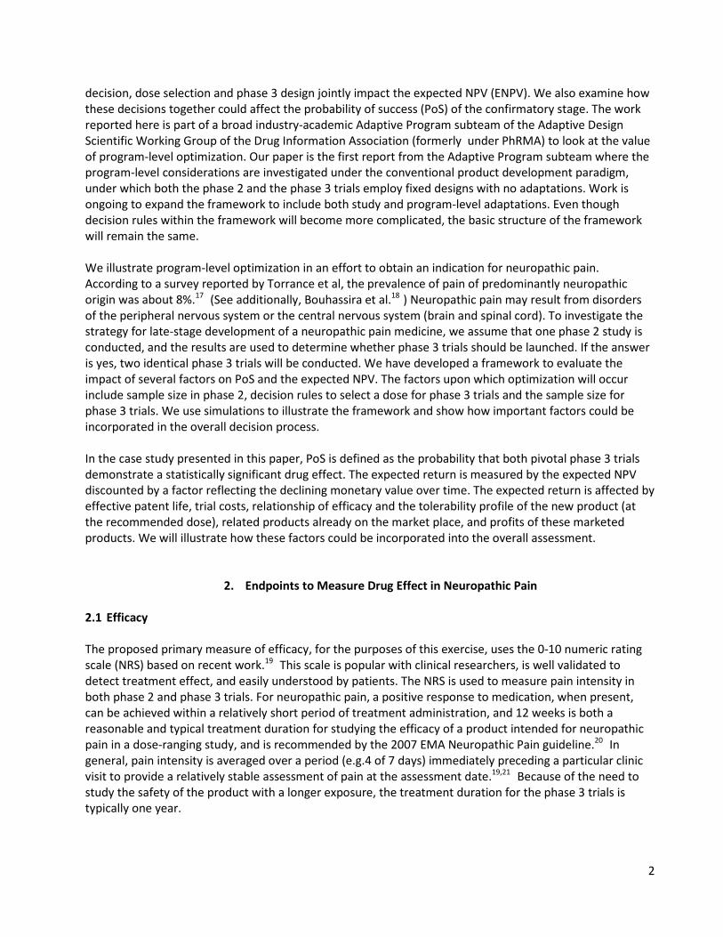
The maximum efficacy in the base case is 1.1. In addition, we will consider maximum efficacy of 0.55 and 1.65. These represent an effect 50% below and 50% above the base case for efficacy. We included in Figure 1 placebo-adjusted dose-response relationships considered in our simulation. Those in Figure 1 with the addition of an “EmaxLow” case were considered by previous researchers.23 Instead of including EmaxLow in our simulation, we considered a series of higher and lower maximum values for each dose-response curve. We also included an exponential dose-response curve which achieves the target level of response at the highest dose. The Explicit curve in Figure 1 is formed by a set of explicitly given data points. All curves in Figure 1 could be approximated by a 4-parameter logistic model (see Section 4.1). All non-null dose-response curves are scaled to have the maximum effect of 1.1. We assume that the dose-response curves for phase 3 trials are the same as those for phase 2. In this paper, we mainly report findings with data produced under the SigmoidEmax relationship. Results from the other efficacy scenarios are available at Cytel’s website http://www.cytel.com/Learn/Publications-DIJPatel-etal-DsgnPh2-Ph3-PoS-NPV-TblsGrphs.aspx.

Figure 1. Dose-response curves considered in the simulation.

3.2 Dose-Response Models for Tolerability Assuming that the rate of clinically meaningful nuisance AEs in the placebo group is 0.1, we consider three AE profiles as described in Table 1. Under the low AE scenario, the rate at the highest dose is 0.175. Under the moderate AE scenario, the rate at the highest dose is 0.35. The corresponding AE rate under the high AE scenario is 0.525. The moderate AE rate scenario is the base case for tolerability.

5

Table 1. Three AE scenarios considered in the simulations. AE Profile Doses

Placebo D1 D2 D3 D4 D5 D6 D7 D8

Low 0.1 0.1 0.1 0.1 0.1 0.1 0.125 0.15 0.175 Moderate 0.1 0.1 0.1 0.1 0.15 0.2 0.25 0.3 0.35

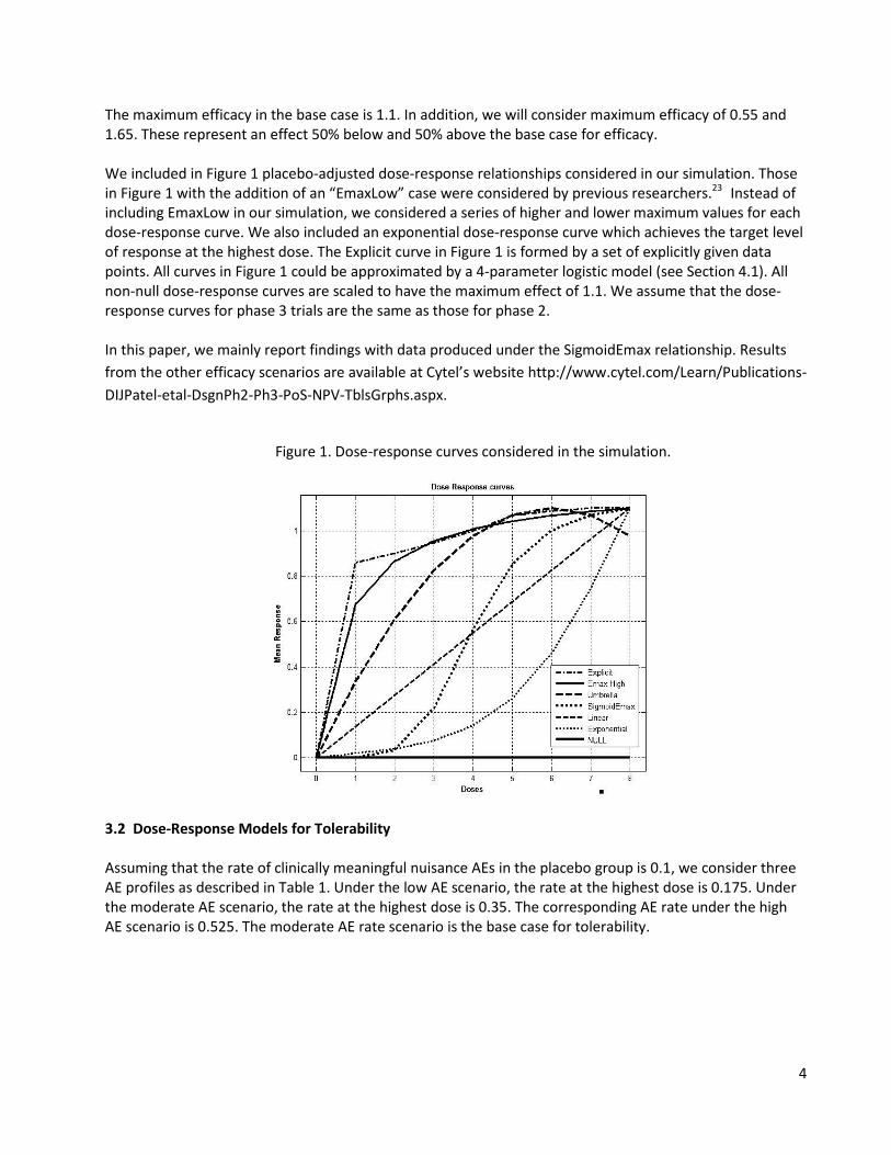
High 0.1 0.15 0.15 0.15 0.225 0.3 0.3 75 0.45 0.525 3.3 Expected 5th Year Net Revenue Let e(Di) denote the true treatment effect (difference in efficacy from placebo) and s(Di) the true nuisance AE rate for dose Di. Table 2 shows the estimated 5th year net revenue in billions of US dollars ($) from marketing a single dose Di that reflects the trade-off between efficacy e(Di) and tolerability s(Di). Table 2 was derived based on consultations with two clinicians experienced in the development and commercialization of neuropathic pain medications. These numbers can also be considered as utility since utility functions have arbitrary origin and scale.26 What will be important is the difference in utility when comparing different doses. Our experts felt that there is utility for a compound with an inferior safety profile if it has a superior efficacy or inferior efficacy and superior safety. This is due to the fact that some patients will tolerate the AE’s and benefit from the better efficacy. For example, when s(Di) = 0.25 and e(Di) = 0.9, the utility is 0.75. On the other hand, when s(Di) = 0.4 and e(Di) = 1.75, the utility is 1. In addition to efficacy and safety, these figures also depend on marketed products and their profits. The values elicited from the experts were smoothed by introducing a grid of points and interpolating between points in each cell of the grid. This results in positive NPV’s for values 0.4< e(Di)< 0.8 and 0.5 <s(Di)< 0.75. The smoothed figures (billions, $USD) are displayed in Figure 2. Table 2. Estimates of 5th year net revenue in dollars (billions) for a marketed dose Di with safety and efficacy profiles given by the column and row profiles.

Efficacy compared to

marketed products

Tolerability compared to marketed products

Stop program: s(Di) > 0.5

Worse: 0.3 ≤ s(Di) ≤ 0.5

Similar: 0.2 ≤ s(Di) < 0.3

Better: s(Di) < 0.2

Stop program: e(Di) < 0.8 0.00 0.00 0.00 0.00

Worse: 0.8< e(Di) < 1.0 0.00 0.25 0.75 1.00

Similar: 1.0 ≤ e(Di) < 1.5 0.00 0.50 1.00 1.50

Better 1.5 ≤ e(Di)

0.25 1.00 1.50 2.00

6

Figure 2. Expected 5th year net revenue (billions, $USD) as a function of the safety and the efficacy profile of the product at the dose marketed.

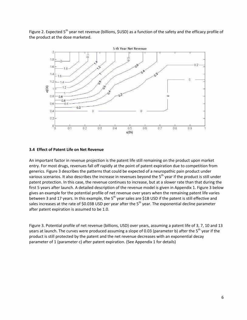
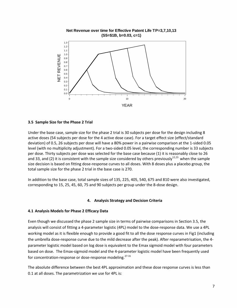
3.4 Effect of Patent Life on Net Revenue An important factor in revenue projection is the patent life still remaining on the product upon market entry. For most drugs, revenues fall off rapidly at the point of patent expiration due to competition from generics. Figure 3 describes the patterns that could be expected of a neuropathic pain product under various scenarios. It also describes the increase in revenues beyond the 5th year if the product is still under patent protection. In this case, the revenue continues to increase, but at a slower rate than that during the first 5 years after launch. A detailed description of the revenue model is given in Appendix 1. Figure 3 below gives an example for the potential profile of net revenue over years when the remaining patent life varies between 3 and 17 years. In this example, the 5th year sales are $1B USD if the patent is still effective and sales increases at the rate of $0.03B USD per year after the 5th year. The exponential decline parameter after patent expiration is assumed to be 1.0. Figure 3. Potential profile of net revenue (billions, USD) over years, assuming a patent life of 3, 7, 10 and 13 years at launch. The curves were produced assuming a slope of 0.03 (parameter b) after the 5th year if the product is still protected by the patent and the net revenue decreases with an exponential decay parameter of 1 (parameter c) after patent expiration. (See Appendix 1 for details)

7

3.5 Sample Size for the Phase 2 Trial Under the base case, sample size for the phase 2 trial is 30 subjects per dose for the design including 8 active doses (54 subjects per dose for the 4 active dose case). For a target effect size (effect/standard deviation) of 0.5, 26 subjects per dose will have a 80% power in a pairwise comparison at the 1-sided 0.05 level (with no multiplicity adjustment). For a two-sided 0.05 level, the corresponding number is 33 subjects per dose. Thirty subjects per dose was selected for the base case because (1) it is reasonably close to 26 and 33, and (2) it is consistent with the sample size considered by others previously12,23 when the sample size decision is based on fitting dose-response curves to all doses. With 8 doses plus a placebo group, the total sample size for the phase 2 trial in the base case is 270. In addition to the base case, total sample sizes of 135, 225, 405, 540, 675 and 810 were also investigated, corresponding to 15, 25, 45, 60, 75 and 90 subjects per group under the 8-dose design.

4. Analysis Strategy and Decision Criteria

4.1 Analysis Models for Phase 2 Efficacy Data

Even though we discussed the phase 2 sample size in terms of pairwise comparisons in Section 3.5, the analysis will consist of fitting a 4-parameter logistic (4PL) model to the dose-response data. We use a 4PL working model as it is flexible enough to provide a good fit to all the dose response curves in Fig1 (including the umbrella dose-response curve due to the mild decrease after the peak). After reparametrisation, the 4-parameter logistic model based on log dose is equivalent to the Emax sigmoid model with four parameters based on dose. The Emax-sigmoid model and the 4-parameter logistic model have been frequently used for concentration-response or dose-response modeling.27-31

The absolute difference between the best 4PL approximation and these dose response curves is less than 0.1 at all doses. The parametrization we use for 4PL is:

NE

T R

EV

EN

UE

0.0

0.1

0.2

0.3

0.4

0.5

0.60.7

0.8

0.9

1.0

1.1

1.2

1.3

YEAR

0 10 20

Net Revenue over time for Effective Patent Life TP=3,7,10,13(S5=$1B, b=0.03, c=1)

8

( | )1 exp

E Y DD

δβθτ

= +

− +

with 0τ > ,

where D is the log dose and Y is the response at that dose. Y is assumed to be normally distributed with variance σ2. If δ > 0, E(Y|D) is monotonically increasing in D with minimum and maximum values of β and β+δ, respectively. Θ is the dose that yields a mean response equal to β + δ/2, the midpoint between the minimum and maximum values. At D= Θ the slope of E(Y|D) is δ/(4τ). For fixed δ, the slope is inversely proportional to τ.

In order to incorporate probability of success calculations into decision-making, we took a Bayesian approach when fitting models to the efficacy data. We assigned “almost flat” priors to the 4 model parameters β, δ, θ , and τ as well as σ2. The priors are independent. They are Normal for β and δ with means equal to 0 and 1.1 respectively with standard deviation = 10. The priors are Uniform (discrete) over a rectangular grid of 30 x 30 points for θ, and τ. The rectangular grid was selected to cover a wide range of values that included the best fit of the dose response curve. σ2 has an Inverse Gamma prior with parameters 0.001 and 1000. We draw samples from the posterior distributions of the five parameters using a Gibbs block sampling algorithm.32 For details see Appendix 2.

4.2 Selection of Dose to Move to Phase 3 Trial For the efficacy endpoint, Gibbs samples from the posterior distribution of e(Di) are used to determine the level of efficacy at Di. For the nuisance AE rate s(Di), we fit an isotonic regression model to the observed AE rates from the simulations. Fitting an isotonic regression model involves pooling estimates of adjacent doses that violate the monotonicity assumption for observed AE rates, so that the estimated AE rates are non-decreasing as a function of the dose.33 We evaluated two methods to select the dose to be studied in the phase 3 trials. The first method chooses the dose estimated to provide efficacy closest to the target efficacy of 1 NRS unit based on the fitted 4PL model. The second method chooses the dose that will have the maximum utility in Table 2 based on efficacy and tolerability estimated from the fitted efficacy and tolerability models. If no dose has an estimated efficacy of 1 unit over the placebo, no phase 3 trials will be conducted under the first method. The second method does not impose any utility threshold to progress to phase 3 other than the minimal requirement that the utility is greater than 0, per the utility function in Table 2. Before either method is applied, we first conduct a linear trend test on the efficacy endpoint. Because doses are equally-spaced on the log scale, the trend test is equivalent to fitting a linear regression model on the log dose. If the trend test is significant at the one-sided 5% level, then we apply the two methods in selecting a dose for phase 3 trials. 4.3 Sample Size Decision for Phase 3 trials When a dose has been identified for the phase 3 trials, two phase 3 trials will be designed with the same sample size. Usually, a phase 3 trial is designed to have a pre-specified power (e.g. 90%) to detect a clinically meaningful difference (e.g. 1 NRS unit) at the two-sided 5% significance level. The standard deviation for the phase 3 trials is assumed to be at 2 units. In our case study, we show how the usual

9

sample size consideration would be overridden by the need to satisfy a requirement of Guideline E1 of the International Conference on Harmonization of Technical Requirements for the Registration of Pharmaceuticals for Human Use (ICH). 4.4 Impact of Compliance with ICH E1 Requirement on Patient Exposure ICH E1 states the extent of pre-marketing product exposure needed to support marketing authorization of drugs intended for long-term treatment of non-life threatening conditions. In general, it is anticipated that the total number of individuals treated with the investigational drug at the dosage levels intended for clinical use should be about 1500. There should be between 300 and 600 patients with at least 6 months drug exposure and at least 100 patients with one year of exposure. In practice, the numbers could be lower or exposure duration reduced in discussions with regulators if there are very good animal data and there is relevant experience with existing drugs having a similar mechanism of action. Similarly, the numbers could be higher and duration longer if there are safety concerns with the drug or the drug is expected to have rapid uptake once it hits the market place. In our case study, we assume that we need 1500 patients treated at the dose of interest, 500 patients treated for at least 6 months and 100 patients treated for at least 1 year. We also assume that dropout rates are such that we would have the necessary number of patients with the required duration if we entered a total of 1500 patients into our Phase 2 (extension phase) and Phase 3 studies at the dose of interest. As the base case, we assume that no other studies except the one phase 2 and two phase 3 trials could contribute to the required safety database. We further assume that patients receiving the investigational product in the phase 2 trial are offered to continue on the investigational product in an extension study at the dose selected for phase 3 trials. These continuing patients will contribute to the required safety database. Thus, if 30 patients per group are enrolled in the 12-week phase 2 study with 8 active doses and if 50% of these 240 patients enter the long-term safety extension study at the dose to be confirmed in phase 3, then at least 120 patients (50% of 30x8) from the phase 2 trial will contribute to the required 1500-patient safety database. The remaining patients will come from the two identical phase III trials. Due to the safety database requirement, phase 3 sample size will be driven by the need to satisfy the safety database requirement in the base case. This safety database requirement results in phase 3 being over-powered for efficacy in every case we have considered. In other words, the sample size for the phase 3 trials has greater than 95% power to detect an effect size of 0.5 at the two-sided 5% significance level. We have also evaluated the case in which a smaller total program sample size is permissible. (See Section 6.5.)

5. Outline of Simulations The simulations can be described as follows Step 1 – Simulate the phase 2 trial under a set of assumptions on doses, sample size per dose, and dose-response relationships for both efficacy and safety. AEs are simulated at each dose using the Binomial distribution while the efficacy data are simulated at each dose using a normal distribution. The efficacy data are modeled using a 4-parameter logistic model while the safety data are analyzed using an isotonic regression model.

10

Step 2 – Based on the results of each simulated phase 2 trial, one dose is chosen to proceed to phase 3 trials using one of the two methods described in Section 4.2. In the case that no dose satisfies the pre-specified criterion under a method, the development program is terminated under that method. Step 3 – In case the development proceeds to phase 3, the sample size for the two (identical) phase 3 studies is determined according to Sections 4.3 and 4.4 (which can vary across scenarios due to the differing sample size contributions of the phase 2 trial participants to the required safety database. Phase 3 data are assumed to follow the same true underlying response distributions as in phase 2. There are three possible outcomes related to the null hypothesis H0 on efficacy, based on phase 3 data:

• H0 is not rejected in either phase 3 trial • H0 is rejected in only one trial • H0 is rejected in both trials

The probability of each of these outcomes is computed analytically using Bayesian conjugate theory. Because of the need to meet the ICH E1 requirement on safety data, the two phase 3 trials are typically over-powered. As such, failure to reject H0 means that the observed efficacy response is very likely to be much lower than the target level, which is 1 unit in this case. When this happens, we assume that resources will not be available to repeat the program to obtain positive data. In this case, the cost of development yields a negative NPV. In the current computations, we did not consider the opportunity cost of not having the resources available for other potential trials. We plan to consider such costs in future work. Step 4 – ENPV is calculated for each simulated run. Many factors affect time and cost estimates (and ultimately, the ENPV calculation). These factors include:

• Total patent life in years • Duration of development time before the phase 2 trial that eats into the patent life • Total number of sites in the phase 2 trial and the average patient accrual rate (per month, per site) • Duration between the completion of phase 2 trial and first subject first visit in the phase 3 trials

(assuming the two phase 3 trials start simultaneously) • Total number of sites for each phase 3 trial and the average patient accrual rate (per month, per

site, per trial) for phase 3 trials (assuming the same figures for both trials) • Duration between the completion of phase 3 trials and product launch • Upfront cost per site and cost per patient • Start-up cost of manufacturing and marketing • Revenue model parameters b and c (See Figure 3) • Discounting rate that reflects the declining monetary value over a year • Minimum number of patients in phase 2 and phase 3 trials needed to fulfill ICH E1 requirement • % of phase 2 subjects expected to complete long-term extension trial

An example of these factors is given in Table 3 below.

Table 3. Time and cost estimates used in ENPV calculations (all costs are in US dollars).

Factors Value Total patent life 17 years

11

Duration of development time prior to phase 2 trial that cuts into the patent life 2 years Patient accrual rate per month per site in the phase 2 trial Total number of sites in phase 2 trial

0.5 50

Time between completion of phase 2 trial and the 1st subject 1st visit in phase 3 trials 6 months Patient accrual rate per month per site in phase 3 trials 1 Total number of sites in each phase 3 trial 80 Time between end of phase 3 trials and product launch 12 months Upfront cost per site Cost per patient Startup cost of manufacturing

1.5K 3.5K 1M

Revenue model parameter b Revenue model parameter c

0.1 0.5

Annual discount rate to be used to calculate ENPV 10% Minimum number of patients per dose in phase 2 and phase 3 trials necessary to satisfy ICH E1 requirement Proportion of phase 2 patients completing 12 month long-term extension trial

1500 50%

Step 5 – Repeat Steps 1-4 500 (or more) times and calculate the following metrics under the set of assumptions and specifications

• Proportion of times when the decision is to move forward to phase 3 development • Proportion of times when phase 3 development is successful • Average total development time in years • ENPV averaged over the simulations • Proportion of simulations in which a safe and efficacious dose as close as possible to best dose) is

selected for phase 3 (If all doses have estimated efficacy < target, in the target method of dose selection then no dose is selected.)

• Proportion of times when ENPV exceeds $100M, $1B, $1.5B, $2B, and $2.5B.

6. Findings from Simulations In this section, we report results from using the specifications in Table 3 with 8 active doses in the phase 2 trial. Except where explicitly noted, SigmoidEmax is assumed to be the true dose-response model. We used 500 simulations for each scenario except for the base case (Tables 4 and 5) where we used 10,000 simulations. 6.1 Impact of Sample Size of the Phase 2 Trial In this sub-section we discuss findings from the base case where the dose-response curve is the SigmoidEmax curve in Fig.1, with the ‘Moderate’ AE profile in Table 1 and the dose selected for phase 3 is the one that is closest to the target efficacy value of 1.0 based on the fitted 4PL model. Table 4 provides results as a function of the sample size in the phase 2 trial. The case of 270 patients (30 per group) is the base case. As the sample size for the phase 2 trial increases, the probability of going into phase 3 increases. A larger phase 2 trial contributes more patients to the safety database, resulting in a smaller phase 3 trial size to meet the ICH E1 requirement. A larger phase 2 trial corresponds to a higher PoS for phase 3. However, it also results in a longer development time and consequently a smaller ENPV. Table

12

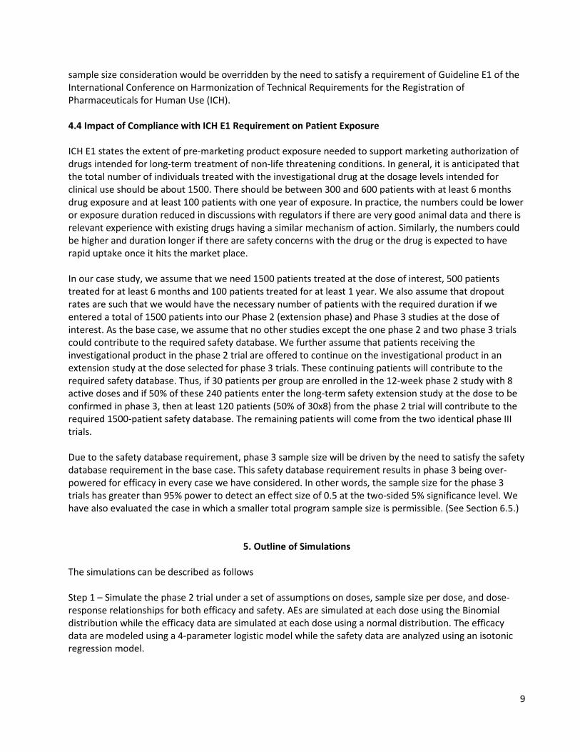
4 shows that the Phase 2 sample size that leads to the highest success probability in phase 3 is 810 whereas the highest ENPV occurs at the sample size of 135 for the target efficacy dose selection method. 6.2 Effect of Dose Selection Method on PoS and Expected NPV We next compare the two methods for selecting the dose for phase 3. One approach selects the dose that is closest to the target efficacy (1.0 on the NRS) based on the fitted 4PL model, and ignores safety. The other method selects the dose that, according to safety and efficacy estimated from the fitted models, will have the highest estimated utility based on Table 2. We compare these two methods with respect to the probability of going into phase 3, phase 3 success probability (PoS), and the ENPV. Table 4. Comparisons between two methods to select the dose for phase 3 development. (10,000 simulations per dose-selection method and sample size )

From Table 4 we see that on all three metrics (Prob. of going to Phase 3, Prob. Phase 3 Success, and ENPV, the method based on maximum utility performs better than selecting the dose based on target efficacy alone. The probability of going to phase 3 is similar across the phase 2 sample sizes for selection based on the target efficacy method while it increases substantially for the utility maximizing method as sample size increases. The reason for similarity for target method is related to the fact that a fixed proportion of the true distribution of the response mean at the target dose lies below the target, and the minimum sample size of 135 is sufficient to estimate this. The improvement in the last column is % of ENPV increase from using the maximum utility method compared to the target efficacy method for the sample size in that particular row of the table. Depending on the phase 2 sample size, the amount of advantage ranges between 66% and 105% for the conditions described in Table 3. This is likely due to the increased probability of starting phase 3; however, it is also a function of the probability of selecting an appropriate dose. Table 4 shows that the optimal sample size (based on ENPV) for the maximum utility method (i.e., 270) is twice that for the target efficacy method. In addition, the ENPV for the maximum utility method at this optimal sample size is twice that of the target efficacy method. We have observed that maximizing utility is superior for all the efficacy and tolerability profiles and sample sizes we have simulated. We therefore focus our discussions on the maximum utility selection method for the remainder of this paper. In this paper we have used ENPV as the financial criterion for optimization as it is the most commonly used method in practice. For smaller companies the objective may be to achieve a milestone of meeting a

Target Dose

Selection

Max Utility Dose

Selection

Target Dose

Selection

Max Utility Dose

Selection

Target Dose

Selection

Max Utility Dose

Selection135 0.81 0.59 0.81 2880 6.7 0.55 0.81 1.22 2.03 66%225 0.95 0.59 0.95 2800 7.0 0.56 0.95 1.16 2.30 98%270 0.97 0.60 0.97 2760 7.1 0.57 0.97 1.15 2.32 101%405 1.00 0.59 1.00 2640 7.5 0.57 1.00 1.10 2.25 104%540 1.00 0.58 1.00 2520 7.9 0.57 1.00 1.04 2.13 105%675 1.00 0.58 1.00 2400 8.3 0.57 1.00 0.98 1.99 104%810 1.00 0.58 1.00 2280 8.6 0.58 1.00 0.92 1.85 100%

ENPV Improve-ment %

Prob. of going to Phase 3

Phase 3 sample

size (both trials)

Total Dev. Time (Yrs)

Prob. Ph 3 Success Expected NPV ($B) Phase 2 Sample

Size

Phase 2 Power

13

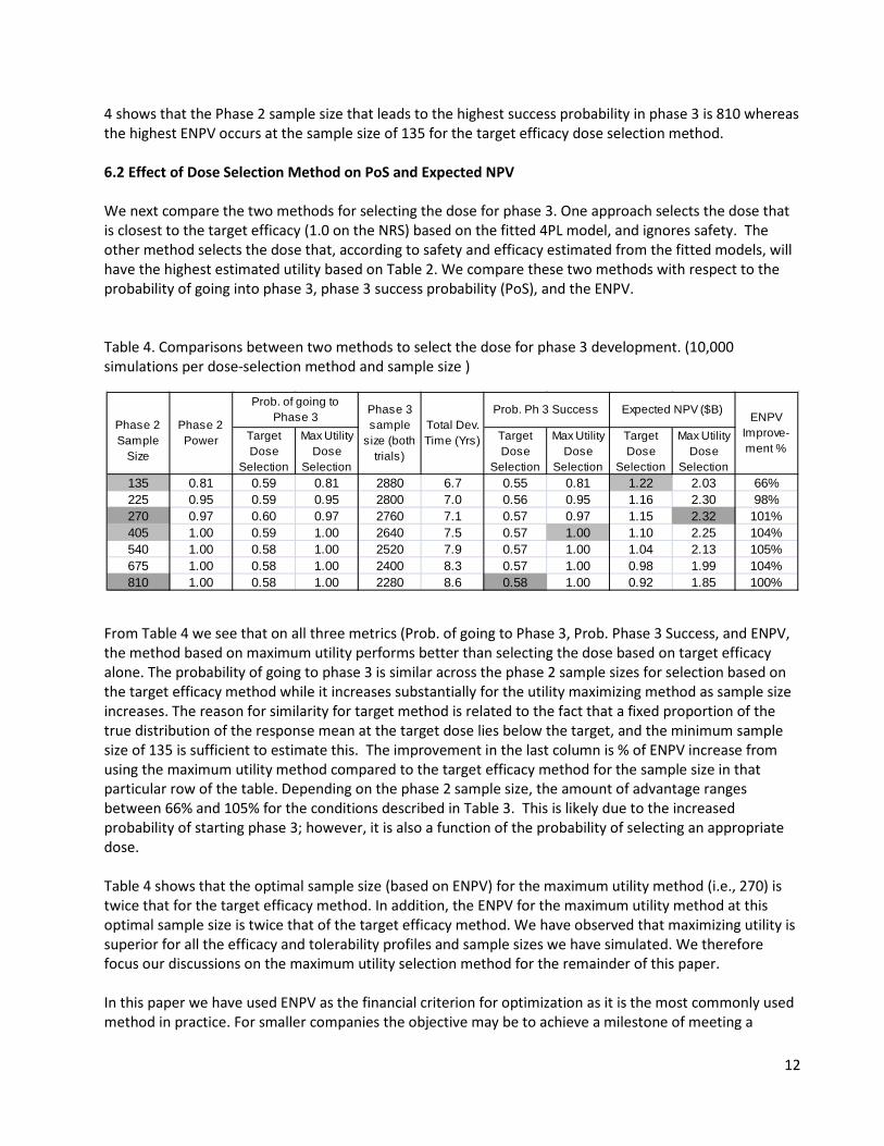
threshold level of NPV. Figure 4 shows the probability of meeting or exceeding various threshold values of NPV for three phase 2 sample sizes for each of the dose selection methods. If the threshold was $2B we see that maximum utility selection method with a sample size of 540 is best. However if the threshold was set at $2.5B it is much better to use a sample size of 135. This is due to the larger sample size lengthening the development time, resulting in reduced chances of reaching high threshold values of ENPV. Note that across all threshold levels and all sample sizes the probabilities are larger for the maximum utility method than for the target efficacy method. Figure 4. Comparing dose selection methods based on probability of exceeding threshold values of NPV (x-axis shows threshold values of NPV($B); y-axis shows probability of exceeding threshold values)

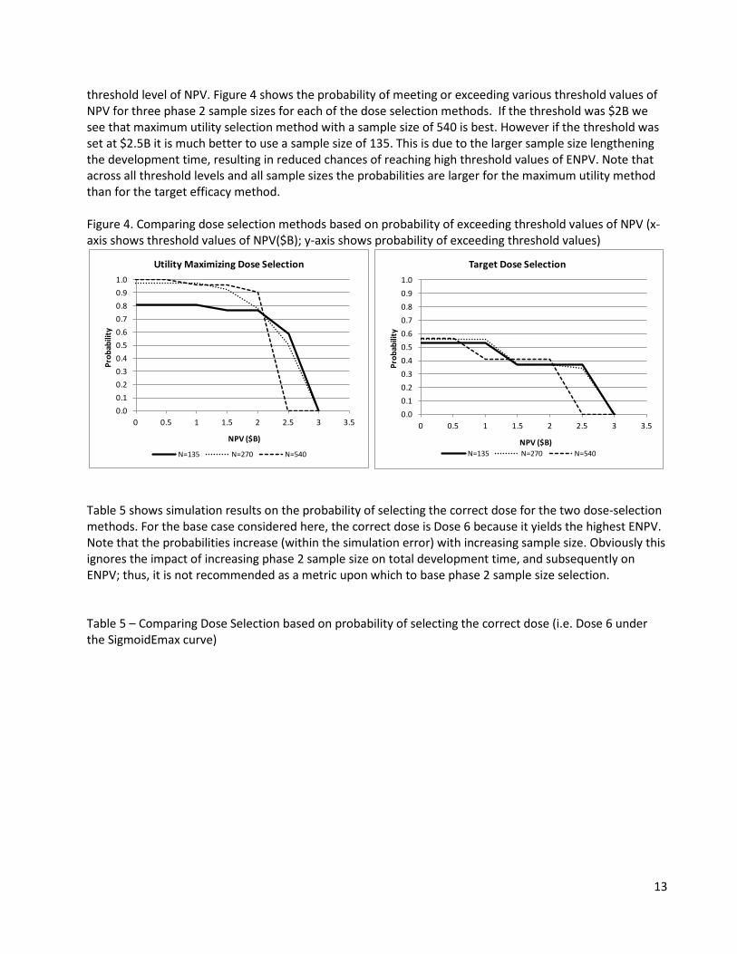
Table 5 shows simulation results on the probability of selecting the correct dose for the two dose-selection methods. For the base case considered here, the correct dose is Dose 6 because it yields the highest ENPV. Note that the probabilities increase (within the simulation error) with increasing sample size. Obviously this ignores the impact of increasing phase 2 sample size on total development time, and subsequently on ENPV; thus, it is not recommended as a metric upon which to base phase 2 sample size selection. Table 5 – Comparing Dose Selection based on probability of selecting the correct dose (i.e. Dose 6 under the SigmoidEmax curve)

0.00.10.20.30.40.50.60.70.80.91.0

0 0.5 1 1.5 2 2.5 3 3.5

Prob

abili

ty

NPV ($B)

Utility Maximizing Dose Selection

N=135 N=270 N=540

0.00.10.20.30.40.50.60.70.80.91.0

0 0.5 1 1.5 2 2.5 3 3.5

Prob

abili

ty

NPV ($B)

Target Dose Selection

N=135 N=270 N=540

14

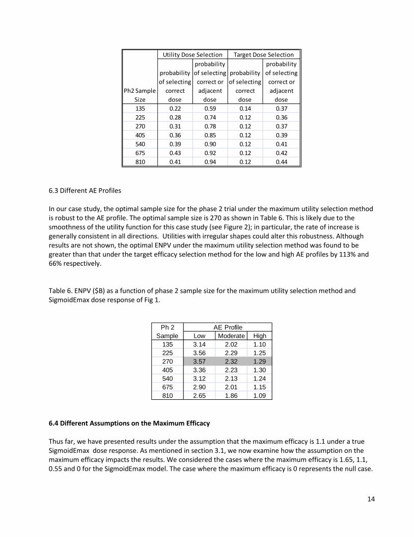
6.3 Different AE Profiles In our case study, the optimal sample size for the phase 2 trial under the maximum utility selection method is robust to the AE profile. The optimal sample size is 270 as shown in Table 6. This is likely due to the smoothness of the utility function for this case study (see Figure 2); in particular, the rate of increase is generally consistent in all directions. Utilities with irregular shapes could alter this robustness. Although results are not shown, the optimal ENPV under the maximum utility selection method was found to be greater than that under the target efficacy selection method for the low and high AE profiles by 113% and 66% respectively. Table 6. ENPV ($B) as a function of phase 2 sample size for the maximum utility selection method and SigmoidEmax dose response of Fig 1.

6.4 Different Assumptions on the Maximum Efficacy Thus far, we have presented results under the assumption that the maximum efficacy is 1.1 under a true SigmoidEmax dose response. As mentioned in section 3.1, we now examine how the assumption on the maximum efficacy impacts the results. We considered the cases where the maximum efficacy is 1.65, 1.1, 0.55 and 0 for the SigmoidEmax model. The case where the maximum efficacy is 0 represents the null case.

probability of selecting

correct dose

probability of selecting

correct or adjacent

dose

probability of selecting

correct dose

probability of selecting

correct or adjacent

dose135 0.22 0.59 0.14 0.37225 0.28 0.74 0.12 0.36270 0.31 0.78 0.12 0.37405 0.36 0.85 0.12 0.39540 0.39 0.90 0.12 0.41675 0.43 0.92 0.12 0.42810 0.41 0.94 0.12 0.44

Utility Dose Selection Target Dose Selection

Ph2 Sample Size

Low Moderate High135 3.14 2.02 1.10225 3.56 2.29 1.25270 3.57 2.32 1.29405 3.36 2.23 1.30540 3.12 2.13 1.24675 2.90 2.01 1.15810 2.65 1.86 1.09

Ph 2 Sample

AE Profile

15

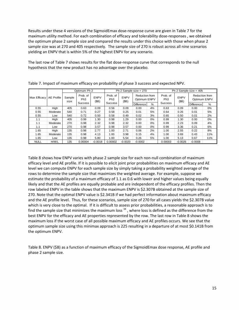
Results under these 4 versions of the SigmoidEmax dose-response curve are given in Table 7 for the maximum utility method. For each combination of efficacy and tolerability dose-responses , we obtained the optimum phase 2 sample size and compared the results under this choice with those when phase 2 sample size was at 270 and 405 respectively. The sample size of 270 is robust across all nine scenarios yielding an ENPV that is within 5% of the highest ENPV for any scenario. The last row of Table 7 shows results for the flat dose-response curve that corresponds to the null hypothesis that the new product has no advantage over the placebo. Table 7. Impact of maximum efficacy on probability of phase 3 success and expected NPV.

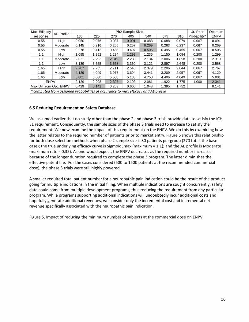
Table 8 shows how ENPV varies with phase 2 sample size for each non-null combination of maximum efficacy level and AE profile. If it is possible to elicit joint prior probabilities on maximum efficacy and AE level we can compute ENPV for each sample size by simply taking a probability weighted average of the rows to determine the sample size that maximizes the weighted average. For example, suppose we estimate the probability of a maximum efficacy of 1.1 as 0.6 with lower and higher values being equally likely and that the AE profiles are equally probable and are independent of the efficacy profiles. Then the row labeled ENPV in the table shows that the maximum ENPV is $2.307B obtained at the sample size of 270. Note that the optimal ENPV value is $2.341B if we had perfect information about maximum efficacy and the AE profile level. Thus, for these scenarios, sample size of 270 for all cases yields the $2.307B value which is very close to the optimal. If it is difficult to assess prior probabilities, a reasonable approach is to find the sample size that minimizes the maximum loss 34 , where loss is defined as the difference from the best ENPV for the efficacy and AE properties represented by the row. The last row in Table 8 shows the maximum loss if the worst case of all possible maximum efficacy and AE profiles occurs. We see that the optimum sample size using this minimax approach is 225 resulting in a departure of at most $0.141B from the optimum ENPV. Table 8. ENPV ($B) as a function of maximum efficacy of the SigmoidEmax dose response, AE profile and phase 2 sample size.

Difference % Difference %0.55 High 405 0.63 0.09 0.56 0.09 0.00 4% 0.63 0.09 0.00 0%0.55 Moderate 540 0.71 0.27 0.58 0.25 0.01 5% 0.64 0.26 0.01 5%0.55 Low 540 0.72 0.50 0.58 0.49 0.02 3% 0.65 0.50 0.01 2%1.1 High 405 0.99 1.30 0.98 1.29 0.00 0% 0.99 1.30 0.00 0%1.1 Moderate 270 0.98 2.32 0.98 2.32 0.00 0% 0.99 2.23 0.09 4%1.1 Low 270 0.98 3.57 0.98 3.57 0.00 0% 0.99 3.36 0.21 6%1.65 High 135 0.98 2.77 1.00 2.71 0.06 2% 1.00 2.55 0.22 8%1.65 Moderate 135 0.98 4.13 1.00 3.98 0.15 4% 1.00 3.69 0.43 11%1.65 Low 135 0.98 5.80 1.00 5.54 0.26 5% 1.00 5.13 0.67 11%

NULL H/M/L 135 0.00004 -0.0018 0.00002 -0.0020 -0.0002 0.00003 -0.0026 -0.0008

Max Efficacy AE Profile

Optimum Ph 2 Ph 2 Sample size = 405

Sample size

Prob. of Ph3

Success

ENPV ($B)

Prob. of Ph3

Success

ENPV ($B)

Reduction from Optimum ENPV

Prob. of Ph3

Success

ENPV ($B)

Reduction from Optimum ENPV

Ph 2 Sample size = 270

16

6.5 Reducing Requirement on Safety Database We assumed earlier that no study other than the phase 2 and phase 3 trials provide data to satisfy the ICH E1 requirement. Consequently, the sample sizes of the phase 3 trials need to increase to satisfy the requirement. We now examine the impact of this requirement on the ENPV. We do this by examining how the latter relates to the required number of patients prior to market entry. Figure 5 shows this relationship for both dose selection methods when phase 2 sample size is 30 patients per group (270 total, the base case); the true underlying efficacy curve is SigmoidEmax (maximum = 1.1); and the AE profile is Moderate (maximum rate = 0.35). As one would expect, the ENPV decreases as the required number increases because of the longer duration required to complete the phase 3 program. The latter diminishes the effective patent life. For the cases considered (500 to 1500 patients at the recommended commercial dose), the phase 3 trials were still highly powered. A smaller required total patient number for a neuropathic pain indication could be the result of the product going for multiple indications in the initial filing. When multiple indications are sought concurrently, safety data could come from multiple development programs, thus reducing the requirement from any particular program. While programs supporting additional indications will undoubtedly incur additional costs and hopefully generate additional revenues, we consider only the incremental cost and incremental net revenue specifically associated with the neuropathic pain indication. Figure 5. Impact of reducing the minimum number of subjects at the commercial dose on ENPV.

135 225 270 405 540 675 8100.55 High 0.050 0.076 0.087 0.091 0.088 0.088 0.079 0.067 0.0910.55 Moderate 0.145 0.216 0.255 0.257 0.269 0.263 0.237 0.067 0.2690.55 Low 0.278 0.412 0.488 0.497 0.505 0.495 0.455 0.067 0.5051.1 High 1.095 1.252 1.294 1.299 1.236 1.150 1.094 0.200 1.2991.1 Moderate 2.021 2.293 2.319 2.233 2.134 2.006 1.858 0.200 2.3191.1 Low 3.139 3.555 3.568 3.360 3.121 2.897 2.648 0.200 3.5681.65 High 2.767 2.755 2.711 2.548 2.379 2.206 2.044 0.067 2.7671.65 Moderate 4.129 4.049 3.977 3.694 3.441 3.209 2.957 0.067 4.1291.65 Low 5.801 5.660 5.538 5.135 4.758 4.406 4.049 0.067 5.801

2.129 2.298 2.307 2.193 2.061 1.922 1.775 1.000 2.341Max Diff from Opt. ENPV 0.429 0.141 0.263 0.666 1.043 1.395 1.752 0.141

Jt. Prior Probability*

Optimum ENPV

ENPV

* computed from assigned probabilities of occurance to max efficacy and AE profile

Max Efficacy response

AE Profile Ph2 Sample Size

17

6.6 Optimizing Phase 2 and Phase 3 Sample Sizes There are situations when an indication is supplemental to existing indications. In this case, there is often a lower minimum requirement on exposure for safety assessment because the product has already been taken by many patients in the market place. In this case, a relevant question is how to plan phase 2 and phase 3 trials to optimize on the metric of choice. Figure 6 below shows how this assessment could be done using ENPV as the basis for optimization. We include in Figure 6 results from both dose selection methods. The curves suggest that a total sample size of approximately 135 (power=0.812) for the phase 2 trial is the best under the target effect method. Under the maximum utility method, ENPV is maximized at a phase 2 sample size of 270 with phase 2 power =0.975. The optimal total sample size for phase 3 (combined over the two trials) is 1000 for the target efficacy method and 700 for the maximum utility method. The corresponding ENPV’s are 1.42 and 2.79 ($B), respectively. The advantage of the maximum utility method over the target efficacy method is a 96% improvement in the ENPV. Figure 6. Optimizing phase 2 and phase 3 trial sizes when there is no minimum requirement on safety database.

0.50.70.91.11.31.51.71.92.12.32.52.72.9

0 500 1000 1500 2000

ENPV

($B)

Min #subjects on selected dose

Effect of Dose Selection Method on ENPV

Target Efficacy Method Utility Maximization Method

0

0.2

0.4

0.6

0.8

1

1.2

1.4

1.6

1.8

2

2.2

2.4

2.6

2.8

3

200 700 1200 1700 2200 2700

ENPV

($B)

Phase 3 Sample Size (both trials)

225

405

540135675810

135

225405

540675810

270

Target Efficacy Method

Utility Maxim. Method

270

18

6.7 Comparison of 4- vs 8-dose Phase 2 Designs Under the SigmoidEmax shape of dose-response curve, optimal sample size for 4 and for 8 doses in the phase 2 design generally leads to a maximum or near maximum utility at Dose 6. As a result, ENPV is generally greater for the 4-dose than for the 8-dose phase 2 design across the 3 different safety profiles for the low efficacy case, but greater for the 8-dose design across the 3 safety profiles for the base case and high efficacy profiles. The differences, however, were relatively small ranging from -$0.2B to +$0.05B.

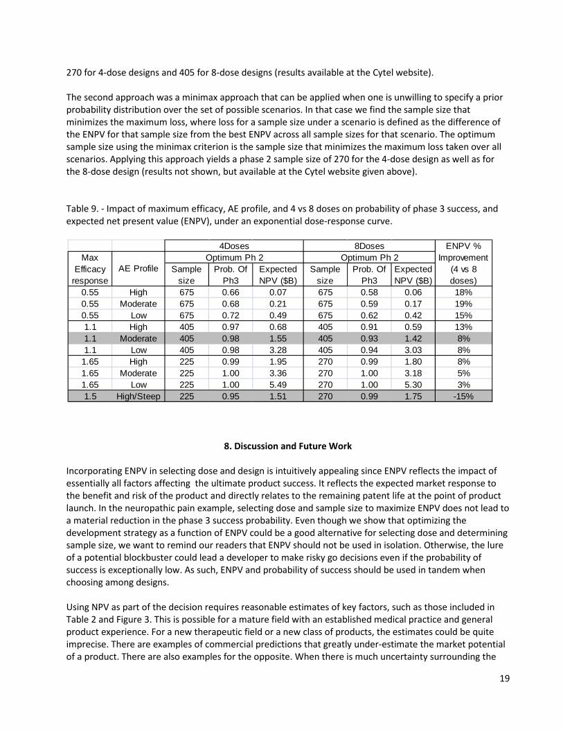
7. Simulation Results for Other Efficacy Dose-Response Curves and the 3 Levels of Tolerability We examined the maximum utility method for dose-selection across other dose-response curves for all combinations of maximum efficacy (i.e., 0.55, 1.1, 1.65) and AE distributions (i.e. low, moderate, high). Similar to the results reported in Section 6.4, the optimal sample size decreased with increasing efficacy level and stayed the same for each tolerability case within each efficacy level (results are available at http://www.cytel.com/Learn/Publications-DIJPatel-etal-DsgnPh2-Ph3-PoS-NPV-TblsGrphs.aspx). Similar to results for the SigmoidEmax curve, the optimal sample size for 4 and for 8 doses in the phase 2 design under other dose-response curves generally lead to the maximum or near maximum utility at or near a dose in the subset of doses 2, 4, 6, and 8. Thus, ENPV is generally greater for the 4-dose design in phase 2 design than for the 8-dose design across different scenarios of max efficacy value and safety profile. This is shown in Table 9 for the exponential dose-response curve (results for other dose-response curves are available at the Cytel website in the paragraph above). The set of dose-response curves studied in this paper can be adequately fit with 4- or 8-dose designs (Section 4.1) because the dose-increment is appropriate to capture the shape. For more extreme cases, which could occur in situations when little knowledge about the potential dose-response curve or appropriate dose-increment to capture the shape exists, the results could be similar to the exceptional case in Section 6.7 where the 8-dose design yielded a greater ENPV than the 4-dose design. The above is illustrated by the case in the last row of Table 9. This case was constructed from the exponential dose-response curve with maximum efficacy 1.1 by shifting the responses one dose to the left, and arbitrarily assigning response 1.5 to Dose 8. We used a tolerability profile as follows: AE rates were 0.1, for placebo and 0.1, 0.1, 0.1, 0.1, 0.12, 0.18, 0.35, and 0.7 for the 8 doses, respectively. This shift in efficacy curves resulted in a reversal of the ENPV advantage between 4 and 8 doses. For the original max efficacy 1.1 / moderate AE rate case (Table 9, row 5), ENVP was 1.55 for the 4-dose phase 2 design and 1.42 for the 8-dose design. However, for the shifted case (bottom of Table 9), ENVP was 1.51 and 1.75 for the 4 and 8 dose designs, respectively. Thus, one needs to be careful in selecting scenarios to study when comparing designs with different numbers of doses. (Results for other dose response curves are not shown here, but can be found at the Cytel website given above). In Section 6.4, we described two approaches to choose sample size for the phase 2 trial when the efficacy dose-response curve had the SigmoidEmax shape. We can readily extend these approaches to situation where there are several shapes for the dose-response curve. In the first approach we elicit a prior probability for each scenario and use these prior probabilities to calculate a weighted average of the ENPV for each sample size. The optimum sample size is the one yielding the highest weighted average ENPV. For example if we believe that the probabilities associated with other shapes are the same as that for the SigmoidEmax shape as given in Table 8 and that all shapes are equally likely, the optimum sample size is

19

270 for 4-dose designs and 405 for 8-dose designs (results available at the Cytel website). The second approach was a minimax approach that can be applied when one is unwilling to specify a prior probability distribution over the set of possible scenarios. In that case we find the sample size that minimizes the maximum loss, where loss for a sample size under a scenario is defined as the difference of the ENPV for that sample size from the best ENPV across all sample sizes for that scenario. The optimum sample size using the minimax criterion is the sample size that minimizes the maximum loss taken over all scenarios. Applying this approach yields a phase 2 sample size of 270 for the 4-dose design as well as for the 8-dose design (results not shown, but available at the Cytel website given above). Table 9. - Impact of maximum efficacy, AE profile, and 4 vs 8 doses on probability of phase 3 success, and expected net present value (ENPV), under an exponential dose-response curve.

8. Discussion and Future Work

Incorporating ENPV in selecting dose and design is intuitively appealing since ENPV reflects the impact of essentially all factors affecting the ultimate product success. It reflects the expected market response to the benefit and risk of the product and directly relates to the remaining patent life at the point of product launch. In the neuropathic pain example, selecting dose and sample size to maximize ENPV does not lead to a material reduction in the phase 3 success probability. Even though we show that optimizing the development strategy as a function of ENPV could be a good alternative for selecting dose and determining sample size, we want to remind our readers that ENPV should not be used in isolation. Otherwise, the lure of a potential blockbuster could lead a developer to make risky go decisions even if the probability of success is exceptionally low. As such, ENPV and probability of success should be used in tandem when choosing among designs. Using NPV as part of the decision requires reasonable estimates of key factors, such as those included in Table 2 and Figure 3. This is possible for a mature field with an established medical practice and general product experience. For a new therapeutic field or a new class of products, the estimates could be quite imprecise. There are examples of commercial predictions that greatly under-estimate the market potential of a product. There are also examples for the opposite. When there is much uncertainty surrounding the

0.55 High 675 0.66 0.07 675 0.58 0.06 18%0.55 Moderate 675 0.68 0.21 675 0.59 0.17 19%0.55 Low 675 0.72 0.49 675 0.62 0.42 15%1.1 High 405 0.97 0.68 405 0.91 0.59 13%1.1 Moderate 405 0.98 1.55 405 0.93 1.42 8%1.1 Low 405 0.98 3.28 405 0.94 3.03 8%

1.65 High 225 0.99 1.95 270 0.99 1.80 8%1.65 Moderate 225 1.00 3.36 270 1.00 3.18 5%1.65 Low 225 1.00 5.49 270 1.00 5.30 3%1.5 High/Steep 225 0.95 1.51 270 0.99 1.75 -15%

4Doses 8Doses ENPV % Improvement

(4 vs 8 doses)

Max Efficacy

responseAE Profile

Optimum Ph 2 Optimum Ph 2Sample

sizeProb. Of

Ph3 Expected NPV ($B)

Sample size

Prob. Of Ph3

Expected NPV ($B)

20

commercial forecast, it is important that a range of utility functions be used to indicate the substantial uncertainty. Although the maximum utility selection method was found to yield higher ENPV’s than the target efficacy selection method for all scenarios reported in the paper, we were cautious in generalizing this finding to a broad conclusion. The scenarios studied in this paper targeted a 1 unit NRS difference from placebo for sizing the phase 2 trial. In practice, a smaller observed statistically significant difference might still trigger a decision to move on to phase 3. The rationale is that, even if the true mean difference from placebo is 1, there is a non-trivial probability of observing a mean difference less than 1. Because of this, we ran simulations for max efficacy response of 1.1 and moderate tolerability, sample sizes from 135 to 810, and decreasing the target efficacy to 0.9, 0.8, … down to 0.2. These all yielded greater ENPV’s for the maximum utility selection method with a minimum advantage of 40 to 60%, depending on sample size, for target 0.8. Thus, the conclusion of higher ENPV associated with the maximum utility selection method appears robust to target value in our case study. The finding of greater ENPV’s for the 4-dose design compared to those for the 8-dose design in most cases studied was surprising. This could have been due to two factors: insufficient number of subjects per dose to make correct dose choice for the 8-dose design and the steepness of the AE dose-response curve assumed in the simulations. On the first point, an adaptive design with 8 doses could increase the number of subjects assigned to the best doses and improve the relative performance of the 8-dose versus the 4-dose design. On the second point, we want to highlight the advantage of the 8-dose design over the 4-dose design for the last case in Table 9, namely a high/steep AE curve. In cases of a steep substantial increase in AE rate, the 8-dose design appears more likely to identify an optimal dose than the coarser 4-dose design. This point was discussed in detail in Section 7. We have deliberately kept the examples and cases in this paper simple. Both phase 2 and phase 3 trials in our reported case study employ fixed designs for a single efficacy endpoint without adaptations. When phase 2 data are promising, we select only one dose and no active comparator for the confirmatory trials. For medications intended for chronic use as is the case with neuropathic pain, it is often desirable to have multiple dosing strengths so that lower doses could be tried first or used to maintain the state stabilized by an initial treatment. This commercially attractive feature, expected to increase the utility of the product, is available for several marketed products for neuropathic pain. We are currently evaluating methods to identify two doses from the phase 2 trial to bring into phase 3 testing.

In addition to assessing methods to carry multiple doses into phase 3 trials, we are also investigating the benefit of adaptations in phase 2 and phase 3 trials. Over the past 10 years, the clinical trial research community has paid increasing attention to adaptive designs. The interest in adaptive designs led to a reflection paper by the Committee for Medicinal Products for Human Use (CHMP) of the European Medicines Agency on Methodological Issues in Confirmatory Clinical Trials Planned with an Adaptive Design and an FDA draft guidance on Adaptive Design Clinical Trials for Drugs and Biologics.35-36 We are currently investigating certain adaptations in phase 2 and phase 3 trials. As could be expected, the more factors there are, the harder it is to assess which factor will have the greatest impact on the metric we wish to optimize. We plan to report on these topics in a follow-up paper.

21

Acknowledgements We would like to thank Carl Fredrik Burman, chair of the Adaptive Programs network of the DIA Adaptive Designs Scientific Working Group and other members of the Working Group who helped shape the approach we describe here, in particular Neal Thomas and Nigel Stallard. Our special thanks went to Keaven Anderson, Zoran Antonijevic, Chris Assaid, Frank Miller, and Narinder Nangia, members of the Neuropathic Pain sub team, for their support and insightful comments. We appreciate the helpful comments from the editorial reviewers; addressing them has improved the manuscript. Finally, we thank Jaydeep Bhattacharya for his excellent programming work in extending the CytelSim software to efficiently execute the simulations.

22

References 1. Hornberger JC, Brown BWM, Halperin J. Designing a cost-effective clinical trials. Statistics in Medicine.

1995;14:2249-2259. 2. Hornberger J, Eghtesady P. The cost-benefit of a randomized trial to a health care organization.

Controlled Clinical Trials. 1998;19:198-211. 3. Chen C, Beckman RA. Optimal cost-effective designs of phase II proof of concept trials and associated

go-no-go decisions. Journal of Biopharmaceutical Statistics. 2009;19:424-436. 4. O’Hagan A, Stevens JW, Campbell MJ. Assurance in clinical trial design. Pharmaceutical Statistics.

2005;4:187-201. 5. Chuang-Stein C. Sample size and the probability of a successful trial. Pharmaceutical Statistics.

2006;5(4):305-309. 6. Chuang-Stein C, Yang R. A Revisit of Sample Size Decision in Confirmatory Trials. Statistics in

Biopharmaceutical Research. 2010;2(2):239-248. 7. Chuang-Stein C, Kirby S, French J, Kowalski K, Marshall S, Smith MK, Bycott P, Beltangady M. A

quantitative approach for making go/no go decisions in drug development. Drug Information Journal. 2011;45:187-202.

8. Julious SA, Swank DJ. Moving statistics beyond the individual clinical trial: applying decision science to

optimize a clinical development plan. Pharmaceutical Statistics. 2005;4:37-46. 9. Burman CF, Grieve AP, Senn S. Decision analysis in drug development. In Dmitrienko A, Chuang-Stein C,

D’Agostino R, eds. Pharmaceutical Statistics Using SAS®: A practical guide. Cary NC: SAS Institute; 2007:385-428.

10. Antonijevic Z. Impact of dose selection strategies on the success of drug development programs. Drug

Information Journal. 2009;4:104-106. 11. Antonijevic Z, Pinheiro J, Fardipour P, Roger JL. Impact of dose selection strategies used in phase II on

the probability of success in phase III. Statistics in Biopharmaceutical Research. 2010;2(4):469-486. 12. Pinheiro J, Sax F, Antonijevic Z, Bornkamp B, Bretz F, Chuang-Stein C, Dragalin V, Fardipour P, Gallo P,

Gillespie W, Hsu CH, Miller F, Padmanabhan SK, Patel N, Perevozskaya I, Roy A, Sanil A, Smith JR. Adaptive and model-based dose-ranging trials: Quantitative evaluation and recommendations (with discussions and rejoinder). Statistics in Biopharmaceutical Research. 2010;2(4):435-454.

13. Kowalski KG, Ewy W, Hutmacher MM, Miller R, Krishnaswami S. Model-based drug development—A

new paradigm for efficient drug development. Biopharmaceutical Report. 2007;15(2):2–22. 14. Kowalski KG, Olson S, Remmers AE, Hutmacher MM. Modeling and simulation to support dose

selection and clinical development of SC-75416, a selective COX-2 inhibitor for the treatment of acute and chronic pain. Clin Pharm Ther. 2008;83:857–866.

23

15. Patel NR, Ankolekar S. A Bayesian approach for incorporating economic factors in sample size and

design for clinical trials and portfolios of drugs. Statistics in Medicine. 2007;26:4976-4988. 16. Mehta CR, Patel NR. Adaptive, group sequential and decision theoretic approaches to sample size

determination. Statistics in Medicine. 2006;25:3250-3269. 17. Torrance N, Smith BH, Bennett MI, Lee AJ. The epidemiology of chronic pain of predominantly

neuropathic origin. Results from a general population survey. J Pain. 2006;7(4):281–9. 18. Bouhassira D, Lantéri-Minet M, Attal N, Laurent B, Touboul C. Prevalence of chronic pain with

neuropathic characteristics in the general population. Pain. 2008;136(3):380–7. 19. Hewitt DJ, Ho TW, Galer B, Backonja M, Markovitz P, Gammaitoni A, Michelson D, Bolognese J, Alon A,

Rosenberg E, Herman G, Wang H. Impact of responder definition on the enriched enrollment randomized withdrawal trial design for establishing proof of concept in neuropathic pain. Pain. 2011;152(3):514-521.

20. EMA Neuropathic Pain guideline. 2007; available at

http://www.ema.europa.eu/docs/en_GB/document_library/Scientific_guideline/2009/09/WC500003478.pdf.

21. Chappell AS, Ossanna MJ, Liu-Seifert H, Iyengar S, Skljarevski V, Li LC, Bennett RM, Harry Collins H.

Duloxetine, a centrally acting analgesic, in the treatment of patients with osteoarthritis knee pain: A 13-week, randomized, placebo-controlled trial. Pain. 2009;146:253-260.

22. Ehrich EW, Davies GM, Watson DJ, Bolognese JA, Seidenberg BC, Bellamy N. Minimal perceptible

clinical improvement with the Western Ontario and McMaster Universities Osteoarthritis Index questionnaire and global assessments in patients with osteoarthritis. J Rheumatol. 2000;27(11):2635-2641.

23. Bornkamp B, Bretz F, Dmitrienko A, Enas G, Gaydos B, Hsu CH, Koenig F, Krams M, Liu Q,

Neuenschwander B, Parke T, Pinheiro J, Roy A, Sax R, Shen F. Innovative approaches for designing and analyzing adaptive dose-ranging trials” (with discussion), Journal of Biopharmaceutical Statistics. 2007;17:965–995.

24. Dragalin V, Hsuan F, Padmanabhan SK. Adaptive designs for dose-finding studies based on sigmoid

Emax model. J Biopharm Stat. 2007;17:1051-1070. 25. Tukey JW, Ciminera JL, Heyse JF. Testing the statistical certainty of a response to increasing doses of a

drug. Biometrics. 1985;41:295-301. 26. Keeney RL, Raiffa H. Decisions with Multiple Objectives: Preferences and Value Tradeoffs. New York,

NY: John Wiley & Sons. 1976. Chapters 4 and 5. 27. Holford N, Sheiner L. Understanding the dose-effect relationship: Clinical application of

pharmacodynamic models. Clin. Pharmacokin. 1981;6:429–453.

24

28. Fedorov VV, Leonov SL. Optimal design of dose response experiments: a model oriented approach. Drug Information Journal. 2001;35:1373–1383.

29. MacDougall J. Analysis of dose-response studies – Emax model. In: Ting N, ed. Dose Finding in Drug

Development. New York, NY: Springer. 2006. Chapter 9. 30. Dragalin V, Bornkamp B, Bretz F, Miller F, Padmanabhan SK, Patel N, Perevozskaya I, Pinheiro J, Smith J.

A simulation study to compare new adaptive dose-ranging designs. Statistics in Biopharmaceutical Research. 2010;2(4):487-512.

31. Miller F, Guilbaud O, Dette H. Optimal designs for estimating the interesting part of a dose-effect

curve. Journal of Biopharmaceutical Statistics. 2007;17:1097-1115. 32. Press SJ. Subjective and Objective Bayesian Statistics: Principles, Models, and Applications, Chapter 6

by Siddhartha Chib. New York, NY: John Wiley & Sons. 2003.

33. Robertson T, Wright FT, Dykstra RL. Order Restricted Statistical Inference. 1988. New York, NY: John Wiley & Sons.

34. Parmigiani G, Inoue LYT. Decision Theory: Principles and Approaches. 2009. Chichester, UK: John Wiley

& Sons. Chapter 7. 35. Committee for Medicinal Products for Human Use. CHMP Reflection Paper on Methodological Issues in

Confirmatory Clinical Trials Planned with an Adaptive Design. Adopted by CHMP on 18 October 2007. Available at www.ema.europa.eu/pdfs/human/ewp/245902enadopted.pdf.

36. FDA draft guidance on Adaptive Design Clinical Trials for Drugs and Biologics. 2010, available at

http://www.fda.gov/downloads/Drugs/GuidanceComplianceRegulatoryInformation/Guidances/UCM201790.pdf.

25

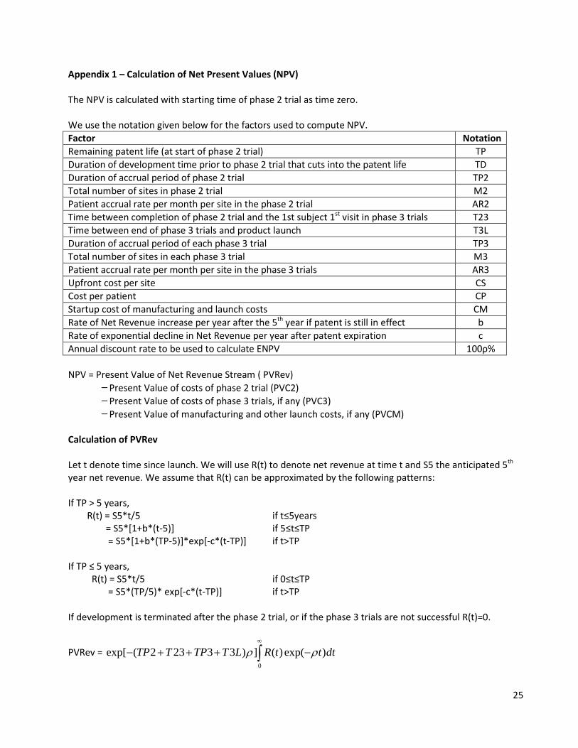
Appendix 1 – Calculation of Net Present Values (NPV) The NPV is calculated with starting time of phase 2 trial as time zero. We use the notation given below for the factors used to compute NPV. Factor Notation Remaining patent life (at start of phase 2 trial) TP Duration of development time prior to phase 2 trial that cuts into the patent life TD Duration of accrual period of phase 2 trial TP2 Total number of sites in phase 2 trial M2 Patient accrual rate per month per site in the phase 2 trial AR2 Time between completion of phase 2 trial and the 1st subject 1st visit in phase 3 trials T23 Time between end of phase 3 trials and product launch T3L Duration of accrual period of each phase 3 trial TP3 Total number of sites in each phase 3 trial M3 Patient accrual rate per month per site in the phase 3 trials AR3 Upfront cost per site CS Cost per patient CP Startup cost of manufacturing and launch costs CM Rate of Net Revenue increase per year after the 5th year if patent is still in effect b Rate of exponential decline in Net Revenue per year after patent expiration c Annual discount rate to be used to calculate ENPV 100ρ% NPV = Present Value of Net Revenue Stream ( PVRev)

Present Value of costs of phase 2 trial (PVC2) Present Value of costs of phase 3 trials, if any (PVC3) Present Value of manufacturing and other launch costs, if any (PVCM)

Calculation of PVRev Let t denote time since launch. We will use R(t) to denote net revenue at time t and S5 the anticipated 5th year net revenue. We assume that R(t) can be approximated by the following patterns: If TP > 5 years, R(t) = S5*t/5 if t≤5years = S5*[1+b*(t-5)] if 5≤t≤TP = S5*[1+b*(TP-5)]*exp[-c*(t-TP)] if t>TP If TP ≤ 5 years, R(t) = S5*t/5 if 0≤t≤TP = S5*(TP/5)* exp[-c*(t-TP)] if t>TP If development is terminated after the phase 2 trial, or if the phase 3 trials are not successful R(t)=0.

PVRev = 0

exp[ ( 2 23 3 3 ) ] ( ) exp( )TP T TP T L R t t dtρ ρ∞

− + + + −∫

26

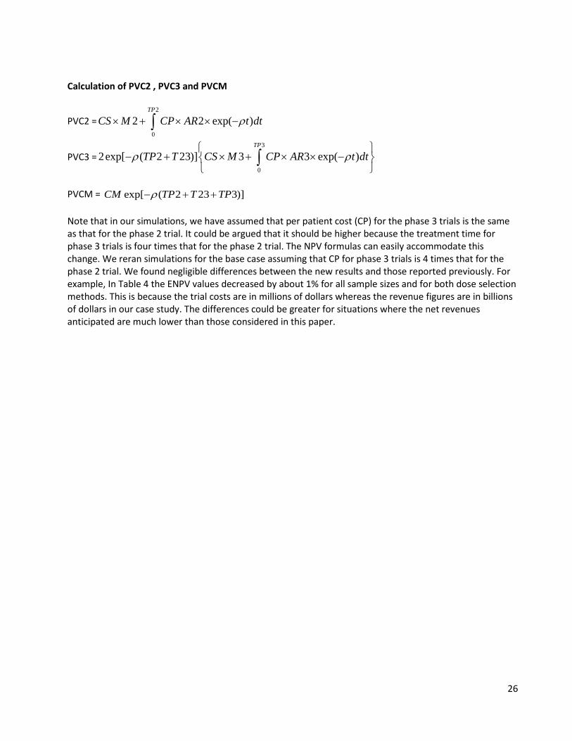
Calculation of PVC2 , PVC3 and PVCM

PVC2 =2

0

2 2 exp( )TP

CS M CP AR t dtρ× + × × −∫

PVC3 =3

0

2exp[ ( 2 23)] 3 3 exp( )TP

TP T CS M CP AR t dtρ ρ

− + × + × × −

∫

PVCM = exp[ ( 2 23 3)]CM TP T TPρ− + + Note that in our simulations, we have assumed that per patient cost (CP) for the phase 3 trials is the same as that for the phase 2 trial. It could be argued that it should be higher because the treatment time for phase 3 trials is four times that for the phase 2 trial. The NPV formulas can easily accommodate this change. We reran simulations for the base case assuming that CP for phase 3 trials is 4 times that for the phase 2 trial. We found negligible differences between the new results and those reported previously. For example, In Table 4 the ENPV values decreased by about 1% for all sample sizes and for both dose selection methods. This is because the trial costs are in millions of dollars whereas the revenue figures are in billions of dollars in our case study. The differences could be greater for situations where the net revenues anticipated are much lower than those considered in this paper.

27

Appendix 2 – Computational Details of MCMC Simulations We assume the following independent priors: β ~ Normal(μβ, σβ

2), δ ~ Normal(μδ, σδ2), θ ~ Discrete Uniform (θL , θL+1 ,⋯ θU),

τ ~ Discrete Uniform (τL , τL+1 ,⋯ τU), the prior for σ2 is ( ) ( )12 2( , ) 1 expInverseGammaα

α ψ σ ψ σ+

∝ −

Let 1 2( , , )T

Dy y y y= be the mean responses observed at doses 1, 2, … D indexed in increasing order

where 1y is the mean response for placebo. Let nj (≥1) be the number of subjects and Dj be the logdose for j = 1, 2, … D. Let W denote the DxD diagonal matrix having 1/nj as the elements on the main diagonal The Gibbs sampling algorithm for sampling from the joint posterior distribution of (β, δ, θ, τ, σ2) is a block sampling algorithm with three blocks consisting of (β, δ), (θ, τ) and σ2. 1. Sample (β, δ|θ, τ, σ2) Let xj = {1+exp(θ – Dj)/τ}−1 and x = (x1, x2,…, xD)T .

Let X denote the Dx2 matrix [1, x] where 1 is the D dimensional column vector consisting of 1’s.

Since jy ~ )/, ( 2jj nxNormal σδβ + independently of ky for k ≠ j, from Bayesian regression theory 32,

we know that

(β, δ|θ, τ, σ2) has a Bivariate Normal distribution

with mean = 1 1 1 1 1

0 0 02 2

1 1( ) ( )T TX W X X W yµσ σ

− − − − −Σ + Σ +

and variance = 1 1 10 2

1( )TX W Xσ

− − −Σ +

2

0 02

00

where and ββ

δδ

µσµ

µσ

Σ = =

Sampling from this Bivariate Normal distribution is the first step in a Gibbs iteration.

2. Sample (θ, τ |β, δ, σ2) The likelihood for θ = θk , τ=τl for θL ≤ θk≤ θU and τL ≤ τl ≤ τU is given by

12

2

1

Pr( | , , , , ) ( | 1 ex p , )D

k jk l

j l j

Dy N y

nθ σθ τ β δ σ β δτ

−

=

− = + +

∏

where (. | , )N ξ η is the univariate Normal distribution with mean ξ and variance η.

28

We compute the likelihood for each support point ( θk , τl) in the discrete prior. Since each point is equally likely in the prior, the joint distribution of (θ, τ) is given by the normalized likelihood obtained by dividing the likelihood at each point by the sum of likelihoods over all points in the grid. We sample the (θ, τ) block by first sampling a value θk from the discrete marginal distribution of θ and then sampling a value τl from the discrete conditional distribution of τ|θk using the inverse cumulative distribution method. 3. Sample (σ2 | θ, τ, β, δ)

Let

21

1 11 expjD n k j

ijj il

DSSQ y

θβ δ

τ

−

= =

− = − − + ∑ ∑

where yij is the response of the ith subject on dose j Since the prior of σ2 is the Inverse Gamma distribution with parameters (α, ψ) it is conjugate to the likelihood of SSQ/σ2 .The posterior distribution of σ2 is thus Inverse Gamma with parameters (α+n/2, ψ +

SSQ/2) with n=1

D

jj

n=∑ .32

We sample σ2 by sampling a random variate from the Gamma distribution with these parameters and then inverting its value.

We have found that using a burn-in sample size of 500 is sufficient to achieve approximate stationarity and we use 1000 Monte Carlo samples after the burn-in for all our simulations.