DESIGNING OF TIME TRUNCATED ACCEPTANCE SAMPLING … · acceptance sampling plan has been one of the...

Electronic Journal of Applied Statistical Analysis EJASA (2013), Electron. J. App. Stat. Anal., Vol. 6, Issue 1, 18 – 31 e-ISSN 2070-5948, DOI 10.1285/i20705948v6n1p18 © 2013 Università del Salento – http://siba-ese.unile.it/index.php/ejasa/index

18

DESIGNING OF TIME TRUNCATED ACCEPTANCE SAMPLING PLANS BY USING TWO-POINT APPROACH

Muhammad Aslam(1)*, Chi-Hyuck Jun(2)

(1)Department of Statistics, National College of Business Administration & Economics, Lahore, Pakistan. (2)Department of Industrial and Management Engineering, Pohang University of Science and Technology,

Republic of Korea

Received 17 August 2011; Accepted 02 April 2012 Available online 26 April 2013

Abstract: We apply the two-point approach to the designing of acceptance sampling plans based on a truncated life test for various life distributions. Two points on the operating characteristic curve are utilized, which are associated with the consumer’s and the producer’s risks. The quality levels are expressed by the ratio of the true mean life to the specified life. The design parameters such as the sample size and the acceptance number will be determined by satisfying two risks at the specified quality levels simultaneously. Tables of design parameters for some selected distributions are prepared according to various levels of the consumer’s risk, test termination time and the quality levels at the producer’s risk. The results are explained with some examples and comparisons are made among the distributions considered.

Keywords: Truncated life test, consumer’s risk; producer’s risk, Gamma distribution, Weibull distribution, generalized Rayleigh distribution.

1. Introduction In order to make a decision on a submitted lot of products about whether to accept or to reject it, a life testing and an acceptance sampling plan are needed. As Pearn and Wu [15] pointed out, acceptance sampling plan has been one of the most practical tools in quality control. It involves quality contracting on product orders between the manufacturers and customers. There are many military standards and international standards such as in [17], [12] and [4] just for the attributes sampling plans. This may demonstrate the practical use of sampling plans. Wherever a sampling plan is used, a more efficient sampling plan is required to be developed and this is the motivation * Email: [email protected]

Aslam, M., Jun, C. (2013). Electron. J. App. Stat. Anal., Vol. 6, Issue 1, 18 – 31.

19

of our study. The efficiency of a sampling plan can be measured by the sample size required and the operating characteristics. In a truncated life testing, it is customary to terminate the experiment as soon as the number of failures is recorded beyond the acceptance number or the time of experiment is reached, whichever comes first when a given number of items (called the sample size) are put on test. To determine an appropriate sample size in this scenario, the usual approach is to fix the acceptance number and to select the sample size that satisfies the specified consumer’s confidence level (or consumer’s risk) when the true mean life equals the specified life (see, for example, [2]). When the lot is accepted, it indicates that the mean life of a product is no shorter than the specified life at a given confidence level. Acceptance sampling plans based on truncated life tests have been proposed by several authors including, for example, [7] for an exponential distribution, [9] for a Weibull distribution, [11] for a Gamma distribution, [10] for normal and lognormal distributions, [19] for a Birnbaum-Saunders distribution, and [2] for a generalized Birnbaum-Saunders distribution. Other authors including [13], [1] and [16] have developed acceptance sampling plans for some other distributions, but, as [2] pointed out, there seems to be some conceptual errors in deriving their results. For the detailed description of various life distributions one may refer to [14]. The approach adopted by the authors mentioned above is basically to use one point on the operating characteristic (OC) curve, which is the consumer’s risk at the given quality level. The manufacturer wants a lot rejection probability less than the producer’s risk at a higher quality level. But, the usual approach may not always satisfy the producer’s risk. Therefore, we need to develop a new method (called two-point approach) based on an acceptance sampling plan satisfying the consumer’s risk at one quality level and the producer’s risk at the other quality level simultaneously. The advantage of two-point approach is that it gives the protection to producer and consumer by minimizing their risk simultaneously. The two-point approach has already been used in designing acceptance sampling plans to control the nonconforming fraction such as in [3] and in constructing variables acceptance sampling plans based on a life test such as in [8]. However, it has not been adopted for designing attributes sampling plans based on a truncated life test. The proposed approach is described in Section 2 and the results for three selected underlying distributions are reported in Section 3. We compared the results from the proposed approach with those from the usual method in Section 4 and concluded in Section 5 with some remarks. 2. Designing by Two-point Approach Suppose that we are using the following single acceptance sampling plan based on a truncated life test: 1) Take a sample of size n from a lot of products and put them on test during a time 0t . 2) Accept the lot if the number of failures during 0t is not larger than c. Truncate the test as

soon as the number of failures observed reaches (c+1) and reject the lot. The plan parameters to be determined in this single sampling plan are the sample size n and the acceptance number c. The criteria to be considered when determining the plan parameters are two things – one is to minimize the sample size and the other is to obtain desirable operating

Designing of Time Truncated Acceptance Sampling Plans by Using Two-point Approach

20

characteristics. The sample size required should be minimized as possible because it is related to the test cost and time. The operating characteristics are expressed by the lot acceptance probability as a function of lot quality. The lot acceptance probability should be lower than the consumer’s risk at an undesirable quality level but it should be higher than (1-producer’s risk) a desirable quality level. Let F be the cumulative distribution function (cdf) associated with the life of a product. Let µ be the mean life and 0µ be the specified life of interest. Assume that the mean life can be obtained from F. Then, the probability that a product fails before time 0t (or unreliability at 0t ), denoted by p , is obtained by:

)( 0tFp = (1) and the lot acceptance probability is given by:

inic

ipp

in

pL −

=

−⎟⎟⎠

⎞⎜⎜⎝

⎛=∑ )1()(

0

(2)

We can express the quality level of a product in terms of the ratio of its mean life to the specified life, i.e., 0/ µµ . The consumer demands that the lot acceptance probability should be smaller than the specified consumer’s risk β at a lower quality level (usually at ratio 1), whereas the producer requires that the lot rejection probability should be smaller than the specified producer’s risk α at a desirably high quality level. Usually, the consumer’s risk is specified by the consumer’s confidence level *P through *1 P−=β . It can be observed that many distributions used for reliability analysis have shape and scale parameters and that each cdf depends on its scale parameter only through the time index. In this case, the failure probability given in (1) is obtained if the ratio of 0/ µµ is specified when the test time is given by 00 µat = with a being a positive constant. For a Weibull distribution with cdf:

))/(exp(1)( γσttF −−= (3) where γ is the known shape parameter and σ is an unknown scale parameter, the failure probability given in (1) is reduced to:

))/(exp(1))/(exp(1 00γγγ µµσ −−−=−−= batp (4)

where:

( )γγγ /)/1(Γ=b (5) When the quality level is expressed by the ratio 0/ µµ , the proposed two-point approach for finding the design parameters determines the sample size and the acceptance number that satisfy the following two inequalities:


21

βµµ ≤= )/|( 10 rpL (6)

αµµ −≥= 1)/|( 20 rpL (7)

where 1r is the mean ratio at the consumer’s risk and 2r is the mean ratio at the producer’s risk. Let 1p be the failure probability corresponding to the consumer’s risk and 2p be the failure probability corresponding to the producer’s risk. 1p is an undesirable quality level that is called as the lot tolerance reliability level (LTRL), whereas 2p is a desirable quality level called the acceptable reliability level (ARL). Then, the two inequalities given in (6) and (7) reduce to:

β≤−⎟⎟⎠

⎞⎜⎜⎝

⎛= −

=∑ inic

ipp

in

pL )1()( 110

1 (8)

α−≥−⎟⎟⎠

⎞⎜⎜⎝

⎛= −

=∑ 1)1()( 220

2ini

c

ipp

in

pL (9)

Note that the existing method usually determines only the sample size with the fixed acceptance number by considering the inequality given in (6) at 11 =r . For the proposed methodology considering the Weibull case, for example, the failure probabilities for both risks are, respectively, given by:

))/(exp(1 11γrabp −−= (10)

))/(exp(1 22

γrabp −−= (11) The mean ratio 2r is the quality level considered as high enough from the producer’s point of view. At a given producer’s risk, a smaller ratio indicates more strict quality requirement from the producer. So, the sample size required will decrease as this ratio increases. 3. Designing Under Some Distributions We will apply the proposed method for determining the design parameters of an acceptance sampling plan to three popularly used life distributions such as the Weibull, Gamma and generalized Rayleigh models. The choice of a distribution should be based on the failure data. Many statistical methods for fitting and estimating a life distribution are available, but these are not the issue of this study. Each of the above three distributions has the shape and the scale parameters and the shape parameter is assumed to be known. It is important to note that the proposed plan is independent of scale parameter of life distribution under transformation

00 µat = . It is only based on the shape parameter of the distribution. Producers usually know the


22

shape parameters of their product. If the shape parameter is unknown, then its estimate should be used from the past experience or the failure data. The failure probability will be derived under each distribution and the design parameters will be determined by the proposed two-point approach. Excel sheets were used to find out the design parameters, which are available from authors upon request. 3.1 The Weibull distribution The Weibull distribution is commonly used in the area of reliability and life data analysis particularly in strength and resistance of materials; see, for example, [8] and [5]. [9] proposed an acceptance sampling plan based on truncated life tests assuming that the life of a product follows the Weibull distribution. The two parameters Weibull distribution with 1=γ reduces to an exponential distribution, which shows that the failure rate is constant over time. When γ =3 or 4, the properties of the Weibull distribution are similar to that of the normal distribution. If the life of parts follows the Weibull distribution, then its mean life can be obtained by:

)/1()/( γγσµ Γ= (12) The failure probabilities for the Weibull case at the consumer’s and the producer’s risks are given by (10) and (11), respectively, which are obtained from (4). Table 1 shows the sample size and the acceptance number chosen for the Weibull distributions with γ =1, 2 and 3. Four consumer’s risks of β =0.25, 0.10, 0.05, 0.01 are considered and

05.0=α is used as the producer’s risk. Two cases of test time are considered, which are a=0.5 and 1.0. The mean ratio at the consumers risk is fixed as 11 =r and various values of the mean ratio at the producer’s risk ( 2r ) are considered. For the case of the exponential distribution, the acceptance number is larger than the acceptance number for γ =2 and 3. For the former case, as the ratio approaches to ten, the acceptance number required approaches to zero. As the shape parameter increases, the required sample size increases when a=0.5, whereas it decreases when a=1.0. Example 1. Suppose that a manufacturer wants to determine the design parameters of an acceptance sampling plan to assure the quality of his product. Assume that the life of a product follows a Weibull distribution with shape parameter of 2 but that the true mean is not known. They would like to accept a lot of products if the true mean is greater than 1,000 hours at the consumer’s risk of 10 percent, whereas the producer’s risk should be less than 5 percent when the true mean is 6,000 hours. For the test time, he wants 500 hours. In this example, the requirements say that 05.0=α , 1.0=β , 62 =r and 5.0=a . So, from Table 1, it is found that

21=n and 1=c . It says that a sample of 21 products should be put on test during 500 hours and the number of failures should be recorded. Accept the lot if there is one or no failures. When the sample size is thought to be too large, the manufacturer should increase the test time instead by taking a smaller sample size.


23

Table 1*. Design parameters for the Weibull distributions when α=0.05. β 0µµ

= 2r Weibull with γ =1 Weibull with γ =2 Weibull with γ =3 a =0.5 a =1.0 a =0.5 a =1.0 a =0.5 a=1.0

0.25 2 37,12 24,13 28,3 11,4 31,1 7,2 3 18,5 13,6 15,1 4,1 ↑ 5,1 4 12,3 7,7 ↑ ↑ 16,0 2,0 5 9,2 ↑ ↑ ↑ ↑ ↑ 6 ↑ ↑ 8,0 2,0 ↑ ↑ 7 ↑ 6,2 ↑ ↑ ↑ ↑ 8 6,1 ↑ ↑ ↑ ↑ ↑ 9 ↑ ↑ ↑ ↑ ↑ ↑ 10 ↑ 4,1 ↑ ↑ ↑ ↑

0.10 2 63,19 37,19 50,5 15,5 61,2 9,2 3 31,8 18,8 29,2 8,2 45,1 7,1 4 22,5 13,5 ↑ ↑ 26,0 4,0 5 15,3 11,4 ↑ 6,1 ↑ ↑ 6 ↑ 9,3 21,1 ↑ ↑ ↑ 7 12,2 ↑ 12,0 3,0 ↑ ↑ 8 ↑ 7,2 ↑ ↑ ↑ ↑ 9 ↑ ↑ ↑ ↑ ↑ ↑ 10 ↑ ↑ ↑ ↑ ↑ ↑

0.05 2 78,23 48,24 64,6 19,6 72,2 10,2 3 37,9 21,9 34,2 10,2 54,1 8,1 4 27,6 16,6 25,1 7,1 34,0 ↑ 5 21,4 14,5 ↑ ↑ ↑ 5,0 6 ↑ 12,4 ↑ ↑ ↑ ↑ 7 18,3 10,3 ↑ ↑ ↑ ↑ 8 14,2 ↑ 16,0 4,0 ↑ ↑ 9 ↑ 8,2 ↑ ↑ ↑ ↑ 10 ↑ ↑ ↑ ↑ ↑ ↑

0.01 2 113,32 68,33 93,8 27,8 115,3 16,3 3 56,13 32,13 53,3 15,3 76,1 10,1 4 40,8 22,8 44,2 12,2 ↑ ↑ 5 33,6 18,6 35,1 9,1 52,0 7,0 6 29,5 16,5 ↑ ↑ ↑ ↑ 7 26,4 14,4 ↑ ↑ ↑ ↑ 8 22,3 12,3 ↑ ↑ ↑ ↑ 9 ↑ ↑ ↑ ↑ ↑ ↑ 10 ↑ ↑ 24,0 6,0 ↑ ↑ *The upward arrow (↑) indicates that the same value of the above cell applies.

3.2 The Gamma distribution The gamma distribution is also widely used in reliability analysis and acceptance sampling plans based on time truncated life tests. The exponential distribution is a special case of the gamma


24

distribution. The applications of the gamma distribution for skewed data can be seen in [6]. For the integer value of the shape parameter, the gamma distribution is called the Erlang distribution. Let )1(≥γ is shape parameter of the gamma distribution and σ is scale parameter of the distribution. The cdf is given as:

!/)/(1)(1

0

/ jtetF j

j

t σγ

σ ∑−

=

−−= (13)

The mean life of the product under the gamma distribution is given by:

γσµ = (14) In the literature, [11] proposed the acceptance sampling plans assuming that the lifetime of the product follows the gamma distribution using the single point approach. The probability of failure of an item before the experiment time under the gamma distribution is given by:

!//

11

0 0

/ 0 jaepj

ja

∑−

=

−

⎟⎟⎠

⎞⎜⎜⎝

⎛−=

γµµγ

µµγ (15)

The probability of failure under the producer’s risk and consumer’s risk (when 11 =r ) given as respectively:

∑−

=

−−=1

01 !/)(1

γγ γj

ja jaep (16)

∑−

=

−−=1

02

/2 !/)/(1 2

γγ γ

j

jra jraep (17)

The plan parameter for the gamma distribution with γ =2 and 3 in Table 2. The plan parameters are determined using the Eq. (16) and Eq. (17) in Eq. (8) and Eq. (9) for other specified same parameter as in Weibull distribution. From the careful observations of the Table 2, we note that as the termination ratio the sample size as well as the acceptance number reduces. We note the same trends in plan parameter when the shape parameter increases from 2 to 3.


25

Table 2*. Design parameters for the Gamma distributions when α=0.05. β 0µµ

= 2r Gamma with γ =2 Gamma with γ =3

a =0.5 a =1.0 a =0.5 a =1.0 0.25 2 27, 5 13, 6 20, 2 8,3

3 14, 2 6, 2 14, 1 4,1 4 10, 1 4, 1 7, 0 ↑ 5 ↑ ↑ ↑ 2,0 6 ↑ ↑ ↑ ↑ 7 5,0 ↑ ↑ ↑ 8 ↑ ↑ ↑ ↑ 9 ↑ 2,0 ↑ ↑ 10 ↑ ↑ ↑ ↑

0.10 2 43,7 19,8 34,3 14,5 3 38,6 14,5 19,1 8,2 4 19,2 8,2 ↑ 6,1 5 14,1 5,1 11,0 ↑ 6 ↑ ↑ ↑ 3,0 7 ↑ ↑ ↑ ↑ 8 ↑ ↑ ↑ ↑ 9 8,0 ↑ ↑ ↑ 10 ↑ ↑ ↑ ↑

0.05 2 52,8 25,10 46,4 18,6 3 32,4 13,4 23,1 9,2 4 22,2 9,2 ↑ 7,1 5 16,1 6,1 ↑ ↑ 6 ↑ ↑ 15,0 ↑ 7 ↑ ↑ ↑ 4,0 8 ↑ ↑ ↑ ↑ 9 ↑ ↑ ↑ ↑ 10 10,0 ↑ ↑ ↑

0.01 2 76,11 35,13 65,5 25,3 3 40,4 18,5 41,2 14,3 4 29,2 13,3 32,1 9,1 5 ↑ 11,2 ↑ ↑ 6 23,1 ↑ 22,0 ↑ 7 ↑ 8,1 ↑ ↑ 8 ↑ ↑ ↑ 6,0 9 ↑ ↑ ↑ ↑ 10 ↑ ↑ ↑ ↑ *The upward arrow (↑) indicates that the same value of the above cell applies.

Example 2. Consider the similar situation as in Example 1. Suppose now that the failure time of the product under inspection follows the gamma distribution with shape parameter of 3. Let consumer’s risk is 25 percent and the experimenter will accept the product if the true mean is


26

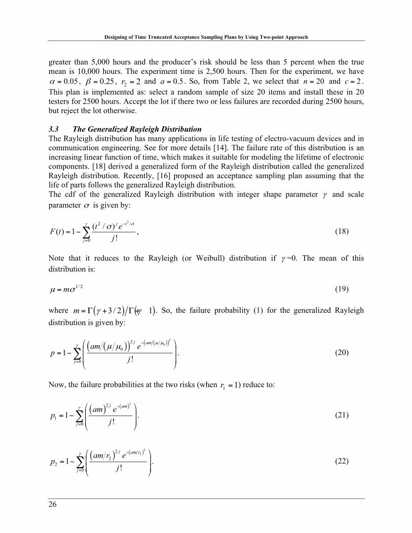
greater than 5,000 hours and the producer’s risk should be less than 5 percent when the true mean is 10,000 hours. The experiment time is 2,500 hours. Then for the experiment, we have

05.0=α , 25.0=β , 22 =r and 5.0=a . So, from Table 2, we select that 20=n and 2=c . This plan is implemented as: select a random sample of size 20 items and install these in 20 testers for 2500 hours. Accept the lot if there two or less failures are recorded during 2500 hours, but reject the lot otherwise. 3.3 The Generalized Rayleigh Distribution The Rayleigh distribution has many applications in life testing of electro-vacuum devices and in communication engineering. See for more details [14]. The failure rate of this distribution is an increasing linear function of time, which makes it suitable for modeling the lifetime of electronic components. [18] derived a generalized form of the Rayleigh distribution called the generalized Rayleigh distribution. Recently, [16] proposed an acceptance sampling plan assuming that the life of parts follows the generalized Rayleigh distribution. The cdf of the generalized Rayleigh distribution with integer shape parameter γ and scale parameter σ is given by:

22 /

0

( / )( ) 1 ,!

j t

j

t eF tj

σγ σ −

=

= −∑ (18)

Note that it reduces to the Rayleigh (or Weibull) distribution if γ =0. The mean of this distribution is:

2/1σµ m= (19) where ( ) ( )3/ 2 1m γ γ=Γ + Γ + . So, the failure probability (1) for the generalized Rayleigh distribution is given by:

( )( ) ( )( )2020

01 .

!

j am

j

am ep

j

µ µγ µ µ −

=

⎛ ⎞⎜ ⎟= −⎜ ⎟⎝ ⎠

∑ (20)

Now, the failure probabilities at the two risks (when 11 =r ) reduce to:

( ) ( )22

10

1 .!

j am

j

am ep

j

γ −

=

⎛ ⎞⎜ ⎟= −⎜ ⎟⎝ ⎠

∑ (21)

( ) ( )2222

20

1 .!

j am r

j

am r ep

j

γ −

=

⎛ ⎞⎜ ⎟= −⎜ ⎟⎝ ⎠

∑ (22)


27

Table 3*. Design parameters for the generalized Rayleigh distribution when α=0.05. β 0µµ

= 2r γ =0 γ =1 γ =2

a =0.5 a =1.0 a =0.5 a =1.0 a=0.5 a=1.0 0.25 2 28,3 11,4 36,1 5,1 42,0 5,1

3 15,1 4,1 19,0 2,0 ↑ 2,0 4 ↑ ↑ ↑ ↑ ↑ ↑ 5 ↑ ↑ ↑ ↑ ↑ ↑ 6 8,0 2,0 ↑ ↑ ↑ ↑ 7 ↑ ↑ ↑ ↑ ↑ ↑ 8 ↑ ↑ ↑ ↑ ↑ ↑ 9 ↑ ↑ ↑ ↑ ↑ ↑ 10 ↑ ↑ ↑ ↑ ↑ ↑

0.10 2 50,5 15,5 52,1 9,2 117,1 6,1 3 29,2 8,2 31,0 6,1 69,0 5,0 4 21,1 6,1 ↑ 4,0 ↑ ↑ 5 ↑ ↑ ↑ ↑ ↑ ↑ 6 ↑ ↑ ↑ ↑ ↑ ↑ 7 12,0 3,0 ↑ ↑ ↑ ↑ 8 ↑ ↑ ↑ ↑ ↑ ↑ 9 ↑ ↑ ↑ ↑ ↑ ↑ 10 ↑ ↑ ↑ ↑ ↑ ↑

0.05 2 64,6 19,6 63,1 10,2 142,1 7.1 3 34,2 10,2 40,0 7,1 90,0 5,0 4 25,1 7,1 ↑ 4,0 ↑ ↑ 5 ↑ ↑ ↑ ↑ ↑ ↑ 6 ↑ ↑ ↑ ↑ ↑ ↑ 7 12,0 ↑ ↑ ↑ ↑ ↑ 8 ↑ 4,0 ↑ ↑ ↑ ↑ 9 ↑ ↑ ↑ ↑ ↑ ↑ 10 ↑ ↑ ↑ ↑ ↑ ↑

0.01 2 93,8 27,8 112,2 16,3 199,1 10,1 3 53,3 15,3 88,1 10,1 138,0 7,0 4 44,2 12,2 60,0 7,0 ↑ ↑ 5 35,1 9,1 ↑ ↑ ↑ ↑ 6 ↑ ↑ ↑ ↑ ↑ ↑ 7 ↑ ↑ ↑ ↑ ↑ ↑ 8 ↑ ↑ ↑ ↑ ↑ ↑ 9 ↑ ↑ ↑ ↑ ↑ ↑ 10 24,0 6,0 ↑ ↑ ↑ ↑ *The upward arrow (↑) indicates that the same value of the above cell applies.

Table 3 shows the sample size required and the acceptance number chosen for the generalized Rayleigh distribution with γ =0, 1 and 2. Other parameter setting is specified same as for the Weibull case.


28

It is seen from this table that the sample size required increases as the shape parameter increases when a=0.5 but that it decreases when a=1.0. Example 3. Now assume that the life of a ball bearing follows a generalized Rayleigh distribution with shape parameter of 1. They would like to accept a lot of ball bearings if the true mean life is greater than the specified life of 10,000 cycles at the consumer’s risk of 10 percent, whereas the producer’s risk should be less than 5 percent when the true mean is 40,000 cycles. The manager is willing to perform the life test during the specified life. In this example, the requirements say that 05.0=α , 10.0=β , 42 =r and 0.1=a . So, from Table 3, it is found that 4=n and 0=c . It says that a sample of 4 bearings should be put on test during 10,000 cycles. Accept the lot if there are no failures. 4. Some Comparisons It may be interesting to see how the sample size varies according to the underlying distribution having the same mean. Table 4 summaries the sample sizes for different mean ratios under various distributions when α=0.05, β=0.1 and a=0.5. Table 5 is a similar table when a=1.0. Table 4. Sample sizes required when α=0.05, β=0.1 and a=0.5.

0µµ = 2r Exponential Weibull with γ =2

Weibull with γ =3

Gamma with γ =2

Gamma with γ =3

Generalized Rayleigh with γ =1

2 4 6 8 10

63 22 15 12 12

50 29 21 12 12

61 26 26 26 26

43 19 14 14 8

34 19 11 11 11

55 31 31 31 31

Table 5. Sample sizes required when α=0.05, β=0.1 and a=1.0.

0µµ = 2r Exponential Weibull with γ =2

Weibull with γ =3

Gamma with γ =2

Gamma with γ =3

Generalized Rayleigh with γ =1

2 4 6 8 10

37 13 9 7 7

15 8 6 3 3

9 4 4 4 4

19 8 5 5 5

14 6 3 3 3

9 4 4 4 4

It is observed that the sample sizes required are generally larger under the generalized Rayleigh distribution than under Weibull or Gamma distributions when the test time is shorter.


29

Table 6. OC values from two approaches for Weibull with γ=2 and a=0.5 β 0µµ = 2r Two-point One-point

( n , c) OC value ( n , c) OC value 0.25 2 28,3 0.9570 8,0 0.6752

3 15,1 0.9594 8,0 0.8398 4 15,1 0.9859 8,0 0.9065 5 15,1 0.9940 8,0 0.9391 6 8,0 0.9573 8,0 0.9573 7 8,0 0.9685 8,0 0.9685 8 8,0 0.9758 8,0 0.9758 9 8,0 0.9808 8,0 0.9808 10 8,0 0.9844 8,0 0.9844

0.10 2 50,5 0.9684 12,0 0.5549 3 29,2 0.9758 12,0 0.7697 4 29,2 0.9948 12,0 0.8631 5 29,2 0.9985 12,0 0.9101 6 21,1 0.9942 12,0 0.9366 7 12,0 0.9531 12,0 0.9531 8 12,0 0.9639 12,0 0.9639 9 12,0 0.9713 12,0 0.9713 10 12,0 0.9767 12,0 0.9767

0.05 2 64,6 0.9669 16,0 0.4559 3 34,2 0.9634 16,0 0.7053 4 25,1 0.9629 16,0 0.8217 5 25,1 0.9837 16,0 0.8819 6 25,1 0.9918 16,0 0.9164 7 25,1 0.9955 16,0 0.9379 8 16,0 0.9521 16,0 0.9521 9 16,0 0.9620 16,0 0.9620 10 16,0 0.9691 16,0 0.9691

0.01 2 93,8 0.9656 24,0 0.3079 3 53,3 0.9725 24,0 0.5924 4 44,2 0.9834 24,0 0.7449 5 35,1 0.9693 24,0 0.8282 6 35,1 0.9844 24,0 0.8773 7 35,1 0.9913 24,0 0.9083 8 35,1 0.9948 24,0 0.9290 9 35,1 0.9967 24,0 0.9435 10 24,0 0.9540 24,0 0.9540

The sample size is smallest under the Gamma distribution with γ =3 among the chosen distributions when the test time is relatively short (a=0.5). However, when the test time is relatively long (a=1) the sample sizes required are quite similar along the distributions.


30

In order to demonstrate the utility of the proposed two-point approach, we compared the results with those from the usual method of determining the design parameters by considering only the consumer’s risk (called one-point method). The Weibull distribution with the shape parameter

2=γ was chosen just for an example, but other life distributions can be considered similarly. The design parameters along with the corresponding OC values were calculated for various mean ratios with the producer’s risk of 5 percent, which were shown in Table 6. It is observed that the two-point approach ensures the quality requirements satisfying the consumer’s and the producer’s risks and that the one-point method cannot provide the sufficient probability of acceptance at some lower mean ratios. The results from both methods become identical when the mean ratio increases. 5. Conclusion The proposed approach can be applied to many other distributions that have not been considered here as long as the unknown scale parameter is represented by its mean or the mean ratio to the specified life. It is concluded that the gamma distribution with shape parameter 3 provides the less sample size as compared to other distributions. Further, even the single-point approach provides the less sample size as compared to the two-point approach but the probability of acceptance may be less than the specified producer’s confidence level. Also, the proposed approach is applicable to design some other sampling plans. A similar approach can be developed for controlling median or some other quality measures instead of mean. Further studies should be needed for economically designing the acceptance sampling plan to determine the sample size and test time simultaneously by considering costs associated with testing each item and with test time. Acknowledgement We would like to thank anonymous referees for their helpful comments in improving our manuscript. References [1]. Baklizi, A., EI Masri, A. E. K. (2004). Acceptance sampling based on truncated life tests in

the Birnbaum- Saunders model. Risk Analysis, 24, 1453-1457. [2]. Balakrishnan, N., Leiva, V., Lopez, J. (2007). Acceptance sampling plans from truncated

life tests based on the generalized Birnbaum-Saunders distribution. Communication in Statistics-Simulation and Computation, 36, 643-656.

[3]. Balamurali, S., Jun, C.-H. (2006). Repetitive group sampling procedure for variables inspection. Journal of Applied Statistics, 33, 327-338.

[4]. BS 6001-0. (1996). Sampling procedures for inspection by attributes-Part 0: Introduction to the BS 6001 attribute sampling system. British Standards Institution.


31

[5]. Chen, J., Chou, W., Wu, H., Zhou, H. (2004). Designing acceptance sampling schemes for life testing with mixed censoring. Naval Research Logistics, 51, 597-612.

[6]. Drenick, R. F. (1960). Mathematical aspects of reliability analysis. Journal of the Society for Industrial and Applied Mathematics, 8, 125-149.

[7]. Epstein, B. (1954). Truncated life tests in the exponential case. The Annals of Mathematical Statistic, 25, 555-564.

[8]. Fertig, F.W., Mann, N.R. (1980). Life-test sampling plans for two-parameter Weibull populations. Technometrics. 22, 165-177.

[9]. Goode, H.P., Kao, J.H.K. (1961). Sampling plans based on the Weibull distribution. In Proceeding of the Seventh National Symposium on Reliability and Quality Control, Philadelphia. 24-40.

[10]. Gupta, S.S. (1962). Life test sampling plans for normal and lognormal distributions. Technometrics, 4, 151-175.

[11]. Gupta, S.S., Groll, P.A. (1961). Gamma distribution in acceptance sampling based on life tests. Journal of the American Statistical Association, 56, 942-970.

[12]. ISO 2859-0. (1995). Sampling procedures for inspection by attributes-Part 0: Introduction to the ISO 2859 attribute sampling system. ISO, Geneva.

[13]. Kantam, R.R. L., Rosaiah, K., Rao, G.S. (2001). Acceptance sampling based on life tests: Log-logistic models. Journal of Applied Statistics, 28, 121-128.

[14]. Marshall, A.W. and Olkin, I. (2007). Life distributions. New York: Springer. [15]. Pearn, W.L., Wu, C.-W. (2006). Critical acceptance values and sample sizes of a variables

sampling plan for very low fraction of defectives. Omega, 34, 90-101. [16]. Tsai, T.-R., Wu, S.-J. (2006). Acceptance sampling based on truncated life tests for

generalized Rayleigh distributions. Journal of Applied Statistics, 33, 595-600. [17]. United States Department of Defense. (1964). MIL-STD 105D. Sampling procedures and

tables for inspection by attributes. Government Printing Office, Washington, D. C. [18]. Voda, V. Gh. (1976). Inferential procedures on a generalized Rayleigh variate, I. Aplikace

Mathematiky, 21, 395-412. [19]. Wu, T-R., Tsai, S-J. (2005). Acceptance sampling plans for Birnbaum-Saunders

distribution under truncated life tests. International Journal of Reliability, Quality and Safety Engineering, 12, 507-519.

This paper is an open access article distributed under the terms and conditions of the Creative Commons Attribuzione - Non commerciale - Non opere derivate 3.0 Italia License.

DESIGNING OF TIME TRUNCATED ACCEPTANCE SAMPLING … · acceptance sampling plan has been one of the...

Documents

Transcript of DESIGNING OF TIME TRUNCATED ACCEPTANCE SAMPLING … · acceptance sampling plan has been one of the...