1

Designing Color Filters that Make Cameras MoreColorimetric

Graham D. Finlayson (g.finlayson@uea.ac.uk) and Yuteng Zhu* (yuteng.zhu@uea.ac.uk)(co-first authors)

Abstract—When we place a colored filter in front of a camerathe effective camera response functions are equal to the givencamera spectral sensitivities multiplied by the filter spectraltransmittance. In this paper, we solve for the filter which returnsthe modified sensitivities as close to being a linear transformationfrom the color matching functions of human visual systemas possible. When this linearity condition - sometimes calledthe Luther condition - is approximately met, the ‘camera+filter’system can be used for accurate color measurement. Then, wereformulate our filter design optimisation for making the sensorresponses as close to the CIEXYZ tristimulus values as possiblegiven the knowledge of real measured surfaces and illuminantsspectra data. This data-driven method in turn is extended toincorporate constraints on the filter (smoothness and boundedtransmission). Also, because how the optimisation is initialised isshown to impact on the performance of the solved-for filters, amulti-initialisation optimisation is developed.

Experiments demonstrate that, by taking pictures through ouroptimised color filters we can make cameras significantly morecolorimetric.

Index Terms—Color filter, camera sensitivity functions, colormeasurement

I. INTRODUCTION

D IGITAL cameras are designed in analogy to the trichro-matic human visual system which has three cone sensors.

If a camera is to capture colors like a human observer,arguably the camera sensors should equal the cone funda-mentals [1]. Practically, however, engineering cameras havingspectral sensitivities similar to the cone fundamentals is onlyrequired if we wished to construct a biologically plausiblemodel of how we see [2]. For most practical applications -e.g. photography and video - it is more important that wecan transform the recorded device RGBs to drive a display sothat the image captured by a camera either looks the same to ahuman observer or records triplets of numbers - e.g. CIE XYZcoordinates - that are referenced to the human visual system[3]. We say that a digital camera is colorimetric if it meets theso-called Luther condition [4], [5], i.e. its spectral sensitivityfunctions are linearly related to the CIE XYZ color matchingfunctions (CMFs).

The Luther condition places a very strong constraint onthe shape of camera spectral sensitivities. A strong constraintis required because the Luther condition effectively assumesthat any and all spectral stimuli are possible. However, manystudies have shown that the actual spectra (measured in the

Graham D. Finlayson and Yuteng Zhu are with the School of Com-puting Sciences, University of East Anglia, NR4 7TJ, Norwich, UK(g.finlayson@uea.ac.uk, corresponding author: yuteng.zhu@uea.ac.uk).

real world) are far from being arbitrary. Indeed, reflectancespectra tend to be quite smooth [6]–[8] and as a consequencecan be fit with low dimensional linear basis [9], [10]. Indeed,spectral basis with dimensions from six to eight, for differentapplications, are often proposed as adequate models of spectralreflectance. Illuminants by contrast are much less describableby small parameter models. Indeed, for artificial lights suchas fluorescent and LED lights, the light spectrum can be veryspiky and the number and position of the spikes can varyconsiderably. And yet, illumninants are also far from beingarbitrary. They are designed to have colors near the Planckianlocus [3], a requirement to score highly on color renderingindices [11].

Possibly, a more practically useful variant of the Luthercondition would be one that is data-driven. That is, wherecamera RGBs can be mapped to XYZs for the spectral datathat are likely to be encountered in the real world. Equally,in principle, we might consider whether a non-linear mappingcould or indeed, should be used.

It is a classical result [12] that if reflectances were exactlymodelled by a 3-dimensional linear model then for a givenlight spectrum there would be a specific 3×3 transform matrixtaking camera RGBs to XYZs. While reflectance spectra arenot adequately described by a 3-dimensional model, RGBscan be approximately mapped to corresponding XYZs usinga 3 × 3 matrix. Indeed, this regression approach is adoptedin almost all cameras with good results (we are mostly happywith the colors a camera records). But, as we shall see laterthe ‘fit’ is not sufficient from a color measurement point ofview.

Of course, rather than using a linear matrix to map RGBs toXYZs, we could use a non-linear transform instead. Possiblenon-linear methods include Polynomial and Root-polynomialregressions and Look-up-tables [13]–[15]. However, the lineartransform method of using a 3 × 3 matrix - even though itis not optimal in terms of fitting error - has two advantagescompared to most non-linear methods. First, the transformscales linearly with exposure. If the scene is made twiceas bright (e.g. by doubling the quantity of incoming light),the same matrix correctly maps the camera measurements toXYZs (because the magnitude of camera RGBs and XYZsboth double). Typically, non-linear methods do not have thisexposure-invariant property (one exception is [16]).

The second advantage is that a linear transform is, well,linear. The human eye measures color stimuli linearly: atthe cone quantal catch level, the response to the sum oftwo spectral stimuli is equal to the sum of the responses

arX

iv:2

003.

1264

5v1

[cs

.CV

] 2

7 M

ar 2

020

2

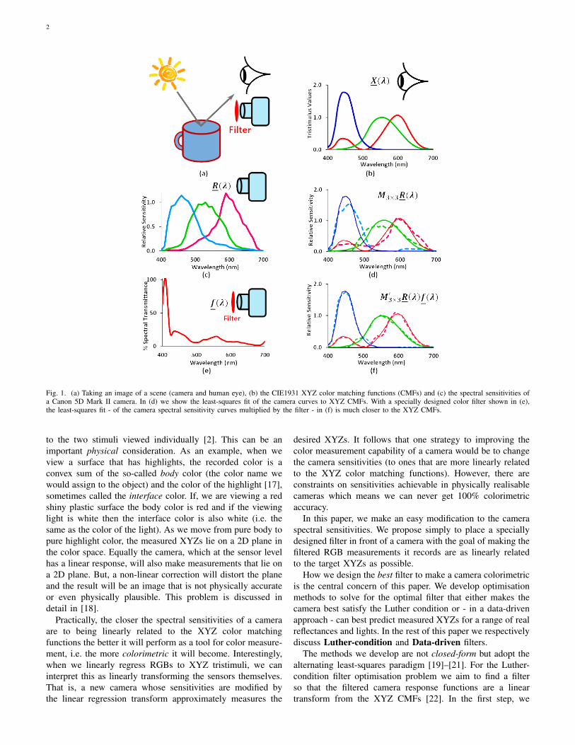
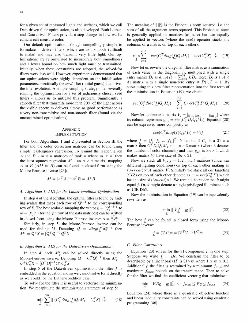
Fig. 1. (a) Taking an image of a scene (camera and human eye), (b) the CIE1931 XYZ color matching functions (CMFs) and (c) the spectral sensitivities ofa Canon 5D Mark II camera. In (d) we show the least-squares fit of the camera curves to XYZ CMFs. With a specially designed color filter shown in (e),the least-squares fit - of the camera spectral sensitivity curves multiplied by the filter - in (f) is much closer to the XYZ CMFs.

to the two stimuli viewed individually [2]. This can be animportant physical consideration. As an example, when weview a surface that has highlights, the recorded color is aconvex sum of the so-called body color (the color name wewould assign to the object) and the color of the highlight [17],sometimes called the interface color. If, we are viewing a redshiny plastic surface the body color is red and if the viewinglight is white then the interface color is also white (i.e. thesame as the color of the light). As we move from pure body topure highlight color, the measured XYZs lie on a 2D plane inthe color space. Equally the camera, which at the sensor levelhas a linear response, will also make measurements that lie ona 2D plane. But, a non-linear correction will distort the planeand the result will be an image that is not physically accurateor even physically plausible. This problem is discussed indetail in [18].

Practically, the closer the spectral sensitivities of a cameraare to being linearly related to the XYZ color matchingfunctions the better it will perform as a tool for color measure-ment, i.e. the more colorimetric it will become. Interestingly,when we linearly regress RGBs to XYZ tristimuli, we caninterpret this as linearly transforming the sensors themselves.That is, a new camera whose sensitivities are modified bythe linear regression transform approximately measures the

desired XYZs. It follows that one strategy to improving thecolor measurement capability of a camera would be to changethe camera sensitivities (to ones that are more linearly relatedto the XYZ color matching functions). However, there areconstraints on sensitivities achievable in physically realisablecameras which means we can never get 100% colorimetricaccuracy.

In this paper, we make an easy modification to the cameraspectral sensitivities. We propose simply to place a speciallydesigned filter in front of a camera with the goal of making thefiltered RGB measurements it records are as linearly relatedto the target XYZs as possible.

How we design the best filter to make a camera colorimetricis the central concern of this paper. We develop optimisationmethods to solve for the optimal filter that either makes thecamera best satisfy the Luther condition or - in a data-drivenapproach - can best predict measured XYZs for a range of realreflectances and lights. In the rest of this paper we respectivelydiscuss Luther-condition and Data-driven filters.

The methods we develop are not closed-form but adopt thealternating least-squares paradigm [19]–[21]. For the Luther-condition filter optimisation problem we aim to find a filterso that the filtered camera response functions are a lineartransform from the XYZ CMFs [22]. In the first step, we

3

find the filter that best maps the spectral sensitivities of thecamera to the XYZ CMFs directly. Then we find the bestlinear combination of the filtered camera sensitivities thatapproximate the XYZ sensitivities. Holding this mapping fixedwe can solve for a new best filter. Then we hold the newfilter fixed to solve for the best linear transform. We iterate inthis way until the procedure converges [23]. Each individualstep in the optimisation can be solved, in closed-form, usingsimple linear least-squares. In the Data-driven approach weanalogously find the filter based on actual measured RGBs andXYZs following the alternating least-squares technique [24].For the Luther- and Data-driven techniques, the constraint thatthe recovered filters must be positive is considered.

Clearly, the filter shown in Fig. 1e is not desireable. In theshort wavelengths there is a sharp change in transmittanceand as a whole the filter is not smooth. For most of thewavelength range the filter transmits little light (<20%).Thus, we extend our optimisation framework to incorporateminimum and maximum bounds on transmittance and alsothat the filters are smooth [25].

Experiments demonstrate that we can find Luther-conditionand Data-driven filters that can dramatically increase the col-orimetric accuracy across a large set of commercial cameras.

The rest of the paper is structured as follows. In Section IIwe review the color matching and color image formation, bothideas underpin our filter design method. The mathematicaloptimisations for the optimal color filter for a given camera arepresented in Section III. The experimental results are reportedin Section IV. The paper concludes in Section V.

II. BACKGROUND

A. Color Matching FunctionsColor matching functions provide a quantitative link be-

tween the physical light stimuli and the colors perceived bythe human vision system. Figure 2 shows a typical setup forthe color matching experiment. The observer views a bipartitefield where one side is lit by a test light while the other side islit by the light mixtures of three primaries (i.e. monochromaticred, green, blue lights). The intensities of three primary lightsare adjusted by the observer to make a visual match, i.e.the two stimuli on each side the bipartite field match if theylook visually indistinguishable to the observer. Sometimes, nomatch is possible. In this case one of the primary lights shouldbe added to the test light field. Mathematically, we can modelthis as if we were subtracting some of the primary light. See[26] for more discussion.

By successively setting the test light to be a unit powermonochromatic light at sample points across the visible spec-trum, we can measure the Color Matching Functions [27].That is we find the RGB mixture that affords a match ona per wavelength basis. Because color matching is linear(the sum of two test spectral lights is matched by the sumof their individual matches) then given the color matchingfunctions we can compute the match for any arbitrary testlight [28]. We simply integrate any test light spectrum withthe Color Matching Functions. It can also be shown that thecolor matching functions are necessarily linearly related to thecone sensitivities [29], [30].

Assuming monochromatic primary lights at 650nm, 530nmand 460nm, the resulting CIE RGB CMFs are shown to theright of Fig. 2. The XYZ CMFs are a linear combination ofthe RGB CMFs, see in Fig. 1b. That XYZ CMFs are used(as opposed to RGB CMFs), in part, because they have, bydesign, no negative sensitivities. Standardised in 1931, the lackof negatives made pencil and paper calculations with matchingcurves easy.

The X, Y and Z scalar values we compute when we integratea test light spectrum with the XYZ CMFs are called XYZtristimuli. In this paper we are interested in using a camera tomeasure XYZ tristimuli.

The color matching experiment is of direct practical impor-tance. Indeed, suppose a display device can output three colorsequal to the R, G and B stimuli used in the color matchingexperiment. It follows that a camera that had sensitivitiesequal to RGB Color Matching Functions would see the correctRGBs to drive the display that would result in a perceptualmatch to the test light. Equally, it would suffice that camera’ssensitivities were linearly related to the CMFs since we couldlinearly transform the camera measurements to the correctRGB to drive the display. Of course, we note that - unlikethe RGB color matching functions - we can only drive theputative display with positive numbers. Consequently, thereare real world colors that cannot be reproduced on displays.

B. Continuous Color Image Formation

The color of a pixel recorded by a digital camera dependson three physical factors: the spectral power distribution ofthe illuminant, the spectral reflectance of the object, and thesensor’s spectral sensitivities. The color formation at a pixel,under the Lambertian surface model, can be modeled as

ρk =

∫ω

E(λ)S(λ)Qk(λ) dλ , k ∈ {R,G,B} (1)

where the subscript k indicates the color channel, λ de-notes wavelength variable defined on the visible spectrum ω(approximately, 400nm to 700nm). The functions E(λ) andS(λ) respectively denote the spectral power distribution of theilluminant and the spectral reflectance. The function Qk(λ) isthe spectral sensitivity of the kth camera color channel.Let us define the color signal C(λ):

C(λ) = E(λ)S(λ). (2)

Substituting Equation (2) into Equation (1):

ρk =

∫ω

C(λ)Qk(λ) dλ , k ∈ {R,G,B}. (3)

C. Discrete Color Image Formation

In the optimisations that will be presented in Section III,it is useful to recast the continuous integrated responsesusing discrete representations where spectra are representedas sampled vectors of measurements. Typically and justifiablyfrom a color accuracy point of view [31], a spectrum can berepresented by 31 measurements made between 400nm and700nm by 10nm sampling interval. Note, the methods we

4

Fig. 2. A typical setup that can be used for the color matching experiment (left). Right shows the CIE 1931 RGB color matching functions obtained fromthe color matching experiments using real R, G, and B primary stimuli.

set forth - since they are designed for the discrete domain- are agnostic about the sampling interval. If the data is givenat a 5nm sampling distance then each spectrum would berepresented as a 61-component vector. Henceforth, we willtalk about spectra being 31-vectors (and this corresponds tothe format of most available measured spectral data).

Equation (3) is now, equivalently, written as:

ρk = C ·Qk, k ∈ {R,G,B}. (4)

Respectively C and Qk

denote the sampled version of the colorsignal spectrum and the kth spectral sensitivity function. Weassume the sampling distance is incorporated in the spectralsensitivity vectors. Here ‘·’ denotes the dot product of twovectors.

One advantage of transcribing image formation into vectornotation is that we can usefully deploy the tools of linearalgebra. Let the matrices C and Q denote 31× n and 31× 3matrices whose columns respectively contain n color signalspectra and the 3 device spectral sensitivities. The n×3 set ofRGB responses can be written as a single concise expression:

P = CTQ, (5)

where T denotes the matrix transpose.Denoting, X as a 31× 3 matrix whose colmuns contain the

discrete XYZ color matiching functions, the XYZ tristimulusresponses can be written as:

X = CT X. (6)

D. The Luther Condition for Camera Spectral Sensitivities

Let us denote individual camera and XYZ responses as ρand x. We can use a camera to exactly measure colors if andonly if there exists a function such that g(ρ) = x for allspectra. It follows that if a pair of spectra integrates to thesame RGB then this pair must also integrate to the same XYZ:

CT1Q = CT

2Q ⇒ CT1 X = CT

2 X (7)

This implies CT1 − C

T2 is simultaneously in the null space

of Q and X. Since any spectrum in the null-space of Q is a

physically plausible spectral difference this implies that thenull-spaces of Q and X are the same and this in turn impliesthe Luther condition

X = QM (8)

where M is a 3× 3 matrix. See [32] for the original proof ofthe Luther condition (which we precis above).

E. The Data-driven Luther Condition

The Luther condition for Spectral Sensitivities presupposesthat any and all physical spectra are plausible. However, weknow that reflectance spectra are smooth [8]. Lights whilemore arbitrary are designed to integrate to fall near or closeto the Planckian locus [3] and to score well on measures suchas the Color Rendering Index [11]. Pragmatically, a camera iscolorimetric if its responses are a linear transformation fromthe XYZ tristimulus values

CT X = CTQM (9)

where M is a 3× 3 matrix.

F. Filter Design

There are many papers in the literature where the spectralsensitivities that a camera should have had are designed [33]–[37]. For example, we can solve for the camera spectral sensi-tivities with respect to which the RGBs mapped with respectto many illuminant spectra can be mapped to correspondingXYZs for a single target illuminant. The procedure wherewe measure colors under a changing light - e.g. in the realworld - but then reference (that is, map) these colors back to afixed illuminant viewing condition is a standard methodologyin color science. Curiously, the best sensors that solve thisproblem are not linearly related to the XYZ CMFs [38].

Perhaps, the closest work to our study is [39]. Here two im-ages are captured. The first with the native spectral sensitivitiesand the second through a colored filter. The emphasis of thatwork was to increase the spectral dimensionality of the capturedevice. Since we make two captures we have 6 measurements

5

per pixel. Effectively we have a 6-dimensional sensor set. Wematch target XYZs by applying a 6 × 3 correction matrix.In [39], the best filter was chosen from a set of commerciallyavailable filters.

There are many other works which propose recoveringspectral information by capturing multiple exposures of thesame scene through multiple filters, e.g. [40]–[44]. A dis-advantage of all these methods is that the capture processis longer and more laborious. Filters need to be changedbetween exposures. The multi-exposure process then need tobe registered. Image registration remains a far from solvedproblem. Moreover, scene elements between exposures maymove (making registration impossible).

The method we propose here is much simpler. We simplyplace a specially designed filter in front of a camera and thentake conventional single exposure images.

III. DESIGNING A FILTER TO MAKE A CAMERA MORECOLORIMETRIC

A. Luther-condition Filters

The Luther condition states that a camera system is col-orimetric if its sensitivities are a linear transform from theXYZ color matching functions. We propose a modified Luthercondition where a camera is said to be colorimetric if thereexists a physically realisable filter which, when placed in frontof the camera, generates effective sensitivities which are alinear transform from the XYZ CMFs.

Physically, the role of a filter, which absorbs light on a perwavelength basis, is multiplicative. If f(λ) is a transmittancefilter and Q(λ) denotes the camera sensitivities then f(λ)Q(λ)is a physically accurate model of the effect of placing a filterin front of the camera sensor.

In Equation (10) we write an optimisation statement for theFilter-based Luther condition:

minf,M‖ diag(f)QM − X ‖2F s.t. f > 0 (10)

Here Q and X are 31 × 3 matrices encoding respectivelythe spectral sensitivities of a digital camera and the CIEstandard XYZ color matching curves. The 31-vector f is thesampled equivalent of the continuous filter function f(λ). Thediag() operation converts a vector into a diagonal matrix (thevector components appear along the diagonal). The meaningof diag(f)Q is the same as f(λ)Q(λ), i.e. the diagonalmatrix allows us to express component-wise multiplication. Mdenotes a 3× 3 matrix. We minimise the square of Frobeniusnorm ‖ ‖2F (we minimise the sum of squares error). Notice theconstraint that the filter value is larger than 0 (physically, wecannot have a filter that has negative transmittance).

We do not have to constrain the maximum transmittancebecause we can only solve for f and M up to an unknownscaling factor. Indeed, suppose the filter f is returned wherethe max transmittance is larger than 1. The fitting error inEquation (10) is unchanged if we divide f by its maximumvalue (resulting in a max transmittance of 100%) so long aswe multiply the corresponding correction matrix M by thesame value.

We minimise Equation (10) using an alternating least-squares (ALS) procedure given in the following algorithm.

Algorithm 1 ALS algorithm for Luther-condition optimisation1: i = 0, Q0 = Q2: repeat3: i = i+ 14: min

fi‖ diag(f i)Qi−1 − X ‖2F

5: minMi‖ diag(f i)Qi−1M i − X ‖2F

6: Qi = diag(f i)Qi−1M i

7: until ‖ Qi −Qi−1 ‖2F < ε8: fLuther =

∏is=1 f

s and M =∏i

s=1Ms

where∏

denotes component-wise matrix multiplication. Steps4 and 5 - where we find the filter and then the linear transform -are solved using simple, closed-form least-squares estimation.For completeness we provide details of how these calculationsare made in the Appendix.

At each iteration, the filter and linear transform - f i andM i - are calculated relative to the previous i − 1 filters andmatrices. It follows in step 8 that the final solution is the multi-plication of all the per-iteration solutions: fLuther =

∏is=1 f

s

(component-wise vector multiplication) and Mj =∏i

s=1Ms

(component-wise matrix multiplication).Notice nowhere in the above procedure do we constrain

the filter transmittance to be larger than 0 (even althoughthis constraint is in the optimisation statement). Empirically,we found that the optimised filter is always positive for allthe cameras we tested (see experimental section). Moreover,Theorem 3.1, presented below, proves that when there existsa filter which makes the camera sensors perfectly colorimetricthat the filter has to be everywhere positive.

The theorem is presented for continuous spectral sensitivityfunctions. As such, we write the XYZ CMFs and camerasensitivities as vector functions: X(λ) and Q(λ). In thisrepresentation, we, effectively, have taken transposes of thematrices Q and X. So, here, we write MT for the 3 × 3matrix. Of course, matrix M in the proof and in the algorithmpresented above signifies the same linear transform.

Theorem 3.1: Assuming there exists an exact solution thatf(λ) > 0 for MTQ(λ)f(λ) = X(λ), the variable λ is definedover the domain where X(λ) > 0 are continuous and fullrank (no one spectral sensitivity can be written as a linearcombination of the other two) and Q(λ) are also continuousthen f(λ) > 0.

Proof: First we remark on the continuity of the cameraand XYZ functions. Both are the result of physical processeswhich are continuous in nature. To our knowledge it isnot possible to make a physical sensor system that captureslight which has discontinuous sensitivities. And, in terms ofphysiological systems, biological sensor response functions arealways continuous.

Next, if f(λ) < 0 across all wavelengths andMTQ(λ)f(λ) = X(λ), then −MTQ(λ) ∗ (−f(λ)) = X(λ).In this case −f(λ) must be all positive and so an all-positive

6

filter can be found. The interesting case to consider is whenthe filter has both negative and positive values.

Clearly the 3 × 3 matrix MT must be full rank otherwisethe mapped camera sensitivities would be rank deficient andtherefore could not model the CMFs. Equally, multiplying bya filter does not change the rank of the sensor set. Because, byassumption Q(λ) are continuous it follows that f(λ) must alsobe a continuous function since otherwise MTQ(λ)f(λ) wouldbe discontinuous (multiplying a continuous and discontinuousfunctions together, save for the case where one of the functionsis everywhere 0, results in a discontinuous function).

As f(λ) is continuous if the function has both negative andpositive values there must be at least one wavelength λv wheref(λv) = 0 and so MTQ(λv)f(λv) = 0. But, this cannot bethe case since the XYZ color matching functions are not allzero at any given wavelength within the defined domain.

QED

B. Data-driven Filters

Simple Case: in the simple Data-driven approach, we lookfor a color filter and the 3 × 3 color correction matrix that,in a least-squares sense, best maps camera measurements fora training color signal data set to the corresponding ground-truth XYZ tristimulus values. Denoting a collection of n colorsignals in the n × 31 color signal matrix C, the Data-drivenoptimisation is written as:

minf,M‖ CT diag(f)QM − CT X ‖2F s.t. f > 0 (11)

Solving Equation (11) depends on the structure of thecolor signal matrix. If we choose C = I31 (the 31 × 31identity matrix) then we can solve this optimisation usingAlgorithm 1 (in this case, Equations (11) and (10) are thesame). This assumption is related to the Maximum Ignoranceassumption [45] where all possible spectra are consideredequally likely.

General Case: Let us develop a more general optimisationstatement. One, where we have cnt color signal matrices- denoted Cj (j ∈ {1, 2, · · · , cnt}) and the correspondingcnt color correction matrices Mj . Each color signal matrixtypically corresponds to a training set of surface reflectancesilluminated by a single spectrum of light Ej , thus the colorsignal matrix is Cj = diag(Ej)S, where S is a 31×n matrixof reflectances, one reflectance spectrum per column. But, thedifferent light assumption is not a necessary assumption. Asan example, we might mix color signals for the MaximumIgnorance assumption with measured data (i.e. two color signalmatrices) where both measurement sets contain multiple lights.

The general Data-driven filter optimisation problem is writ-ten as:

minf,Mj

cnt∑j=1

‖ CTj diag(f)QMj − CT

k X ‖2F s.t. f > 0 (12)

and is solved using Algorithm 2.Finally, k could denote some other privileged standard

reference viewing condition (where the reference viewing

Algorithm 2 ALS algorithm for the Data-driven optimisation

1: i = 0, f0 = fseed, Q0 = diag(f0)Q2: repeat3: i = i+ 14: min

Mij

‖ CTj Q

i−1j M i

j − CTk X ‖2F , j = 1, 2, ..., cnt

5: minfi

∑cntj=1 ‖ CT

j diag(f i)Qi−1j M i

j − CTk X ‖2F , f

i > 0

6: Qij = diag(f i)Qi−1

j M ij

7: until ∀(j) ‖ Qij −Q

i−1j ‖2F < ε

8: fData =∏i

s=0 fs and Mj =

∏is=1M

sj

illuminant is not in the set of training lights). For example,in color measurement we are often interested in the XYZtristimuli for a daylight illuminant D65 which has a prescribedbut not easily physically replicable spectrum.

We are going to solve Equation (12) for the filter f usingan alternating least-squares procedure. Notice that the inputto the optimisation is an initial filter guess denoted by fseed.Let us consider 3 candidate minimisations corresponding to 3common scenarios for color measurement each of which canbe solved using Algorithm 2.1) Multiple Lights: Here we assume that j indexes over cntilluminants and k = j (per illuminant we make the targetXYZs using the same color signals). We find a single filterwhich given per-illuminant optimal least-square 3× 3 correc-tion matrices will best fit camera data to the correspondingmulti-illuminant XYZs.2) Multiple measurement lights, single target light: Againj indexes over cnt illuminants. But, the target is a singleilluminant, for example CIE D65 [3].3) Single Light. This case is, in effect, the simple restrictionof the general case, cnt = 1. We have one measurement lightand one target light. Like the Luther-condition optimisation,we solve for a single correction matrix.

In Algorithm 2, it is straightforward to solve for the jthcolor correction matrix at iteration step i, M i

j , in step 4 usingthe Moore-Penrose inverse. Step 5, where we find the filter,can also be solved directly using simple least-squares, althoughthe basic equations need to be rearranged. Details of theleast-squares computation are given in the Appendix. Here,to ensure that the filter is all positive we can also solve forthe filter by solving the optimisation subject to the positivityconstraints, we solve a quadratic programming problem [46](unlike the Luther-condition case there is no a prior physicalreason why the best filter should be all positive).

Quadratic programming allows linear least-squares problemsubject to linear constraints to be solved rapidly and, crucially,a global optimum is found.

C. Adding Filter Constraints

By default the filter found using Algorithm 2 can be arbi-trarily non-smooth and might also be very non-transmissive.Non-smoothness limits manufacturability (at least with dyebased filters) and a filter that absorbs most of the incominglight would, perforce, have limited practical utility. Both these

7

problems can be solved by placing constraints on the filteroptimisation.

Let us now constrain the target filter f according to:

f = Bc, s.t. fmin ≤ f ≤ fmax (13)

here B denotes a 31 × m basis matrix with each columnrepresenting a basis and the vector c denotes an m-componentcoefficient vector. The scalars fmin and fmax denote lowerand upper thresholds on the desired transmittance of the filter;specifically, fmax is set to 1 by default as fully transmissiveand fmin is a positive value between 0 and 1. Equation (13)forces the optimised filter to be in the span of the columnvectors of B and to meet the min and max transmittanceconstraints. By judicious choice of the basis we can effectivelybound the smoothness of the filter. For example, we couldchoose the first m terms of the discrete cosine transform basisexpansion [47].

With respect to the new filter representation, we rewrite thenew overall filter design optimisation in Equation (12) as

minc,Mj

cnt∑j=1

‖ CTj diag(Bc)QMj−CT

k X ‖2F , fmin ≤ Bc ≤ fmax

(14)The current minimisation can be solved using the same alter-nating least-squares paradigm of Algorithm 2. But, in step 5,we need to substitute the constraint f i > 0 with

fmin ≤ diag(

i−1∏s=0

fs)f i = Bci ≤ fmax (15)

That is, the filter we find at the ith iteration when multipliedby all the filters from the previous iterations is constrained tobe in the basis B.

Looking at Equation (15) we see that

f i = [diag(

i−1∏s=0

fs)]−1Bci (16)

That is, effectively the basis for the ith filter changes at eachiteration. Again we can solve step 5 subject to the constraintsof Equation (16) using Quadratic Programming.

Finally, we note that we could, of course, rewrite Algorithm2 so that at each iteration we solve for a filter defined bya coefficient weight directly (we could solve for an m-termcoefficient vector rather than a 31-component filter). The twoformalisms are equivalent. Here, we chose to solve for theper iteration filter for notational convenience: we can use thegeneral Data-driven algorithm and simply change how wecalculate the per iteration filter optimisation.

D. Initialising the Data-driven Optimisation

Alternating least-squares is guaranteed to converge but itwill not necessarily return the global optimal result. But, it isdeterministic. So, given the state of the correction matrices andfilter at the ith iteration we will ultimately arrive at the samesolution. Equally, if we change the initialisation condition,fseed, in Algorithm 2, we may end up solving for a differentfilter. Empirically, we observed that the filter returned by the

algorithm depends strongly on the initial filter that seeds theoptimisation.

Let us consider 3 different ways to seed the Data-drivenoptimisation:1) Default: fseed = 1. This uniform unit vector denotes a fullytransmissive filter over the spectrum.2) Luther filter: fseed = fLuther. That is we seed the Data-driven optimisation with the optimal Luther-condition filterfound using Algorithm 1.3) By sampling: Here we find a set of sample filters F(which meet our smoothness and transmittance boundednessconstraints) and for each filter sample, f ∈ Fseed, we will runAlgorithm 2.

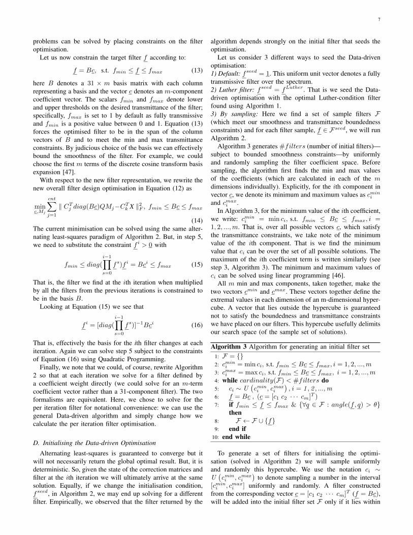
Algorithm 3 generates #filters (number of initial filters)—subject to bounded smoothness constraints—by uniformlyand randomly sampling the filter coefficient space. Beforesampling, the algorithm first finds the min and max valuesof the coefficients (which are calculated in each of the mdimensions individually). Explicitly, for the ith component invector c, we denote its minimum and maximum values as cmin

i

and cmaxi .

In Algorithm 3, for the minimum value of the ith coefficient,we write: cmin

i = min ci, s.t. fmin ≤ Bc ≤ fmax, i =1, 2, ...,m. That is, over all possible vectors c, which satisfythe transmittance constraints, we take note of the minimumvalue of the ith component. That is we find the minimumvalue that ci can be over the set of all possible solutions. Themaximum of the ith coefficient term is written similarly (seestep 3, Algorithm 3). The minimum and maximum values ofci can be solved using linear programming [46].

All m min and max components, taken together, make thetwo vectors cmin and cmax. These vectors together define theextremal values in each dimension of an m-dimensional hyper-cube. A vector that lies outside the hypercube is guaranteednot to satisfy the boundedness and transmittance constraintswe have placed on our filters. This hypercube usefully delimitsour search space (of the sample set of solutions).

Algorithm 3 Algorithm for generating an initial filter set1: F = {}2: cmin

i = min ci, s.t. fmin ≤ Bc ≤ fmax, i = 1, 2, ...,m3: cmax

i = max ci, s.t. fmin ≤ Bc ≤ fmax, i = 1, 2, ...,m4: while cardinality(F) < #filters do5: ci ∼ U

(cmini , cmax

i

), i = 1 , 2 , ...,m

6: f = Bc , (c = [c1 c2 · · · cm]T )7: if fmin ≤ f ≤ fmax & {∀q ∈ F : angle(f, q) > θ}

then8: F ← F ∪ {f}9: end if

10: end while

To generate a set of filters for initialising the optimi-sation (solved in Algorithm 2) we will sample uniformlyand randomly this hypercube. We use the notation ci ∼U(cmini , cmax

i

)to denote sampling a number in the interval

[cmini , cmax

i ] uniformly and randomly. A filter constructedfrom the corresponding vector c = [c1 c2 · · · cm]T (f = Bc),will be added into the initial filter set F only if it lies within

8

the transmittance bounds and it is sufficiently far from thosefilters already in the set, see step 7. In algorithm 3 sufficientlyfar means at least θ degrees from the other set members. Thefunction cardinality() returns the number of members in aset.

IV. RESULTS

A. Experiments for Luther-condition Optimised Filters

Let us return to the example shown in Fig. 1. The optimalLuther-condition filter solved using Algorithm 1 is shown inFig. 1e. We multiply the camera sensors by this filter andthen find the linear least-squares transform mapping the neweffective sensitivities to the XYZ matching functions. Thefitted filtered camera sensitivities (to the XYZ color matchingfunctions) are shown Fig. 1f. In contrast, Fig. 1d, showsthe native camera spectral sensitivities fitted to the XYZs.Visually, the addition of our derived filter makes the cameramuch more colorimetric.

The reader will notice that the filter, Fig. 1e, absorbs morethan 80% of the light except at the shortest wavelengths whereit is maximally transmissive. This need not be a problem forcolor measurement as we can increase exposure time, forexample. Though, it does mean that the camera with andwithout the filter would, for the same recording conditions,capture significantly less light. And, this could result in anincrease in the noise in the final image output by a camerareproduction pipeline. Indeed, if we deploy this filter - andkeep the capture conditions the same - we would need to‘scale up’ the recorded values and this operation also scalesup the noise. Effectively, we capture an image at a higher ISOnumber.

B. Vora-Values

To quantitatively measure the spectral match between thefiltered and linear transformed camera sensors and the XYZcolor matching functions, we calculate the Vora-Value [48].The Vora-Value measures the closeness between the spacesspanned by a set of filter sensitivities set Q and that by thecolor matching functions X. It is defined as

ν(X, Q) =Trace(QQ+XX+)

3(17)

where Trace() returns the sum of the diagonal of a matrixand + is the Moore-Penrose inverse (see Appendix). The Vora-Value is a number between 0 and 1 where 1 indicates the twosensitivity sets span the same space, i.e. the Luther conditionis fully satisfied. While there is not a guide on what differentVora-Values mean, empirically we have found when the Vora-Value is respectively larger than 0.95 and 0.99 then we haveacceptable and very good color measurement performance. Anexplanation of why the Vora-Value is useful for quantifying thecolor measurement potential of a set of color filters togetherwith its derivation can be found in [48].

The Vora-Value performance for a set of 28 camera spectralsensitivities [49] - with and without their optimised filters- are shown in Fig. 3. The Vora-Value for the unfiltered,

Fig. 3. Spectral match to Luther-condition by (a) unfiltered NATive sensitiv-ities and (b) filtered LUTHer-condition optimised sensitivities for a group of28 cameras in terms of Vora-Values. The overall average Vora-Values of thecamera group by both conditions are shown in the green box.

NATive sensitivities are shown in blue and for the LUTHer-condition optimised sensitivities in red. On average, the nativeVora-Value is 0.918 but when the optimised filter is added itincreases to 0.961. This digital cameras data set [49] comprisesof diverse camera types, including professional DSLRs, point-and-shoot, industrial and mobile cameras.

Note, we make a distinction between using a camera forcolor measurement and for making attractive looking images.Here, we are interested in using a camera to measure XYZtristimuli (or measures like CIE Lab values that are derivedfrom tristimuli [3]). From a measurement perspective, we needhigher tolerances and a higher Vora-Value. Clearly, from thepoint of view of making attractive images cameras that haveVora-Values less than 0.95 can work very well. Indeed, manyof the 28 cameras with Vora-Values less than 0.95 can still takeimages that look appealing from a photographic perspective.But, commercial cameras are not suitable vehicles for accuratecolor measurement. Quantitative color measurement results arepresented in the next section.

C. Color Measurement Experiments

Now let us evaluate the derived Luther-condition and Data-driven filters in terms of a perceptually relevant color mea-surement/image reproduction metric. The CIELAB ∆E∗

ab [3]- the Euclidean distance calculated between two tristimuli - isa single number that roughly correlates with the perceived per-ceptual distance between two colors. One ∆E∗

ab correspondsapproximately to a ‘Just Noticeable Difference’ to a humanobserver [27]. When ∆E∗

ab is less than 1 we say that thedifference is imperceptible to the visual system.

1) Single Light Case: Let us use the Canon 5D Mark IIcamera spectral sensitivities as a putative measurement deviceand quantify how well it can measure colors - with and withouta filter. In this experiment the measurement light is eithera CIE D65 (bluish) or a CIE A (yellowish) illuminant. Forreflectances we use the SFU set of 1995 spectra [50] (itselfa composite of many widely used sets). The 1995 XYZs forthese reflectance and lights are the ground-truth with respectto which we measure color measurement error.

Using the Canon camera sensitivities, the reflectance spectraand either the CIE D65 and A lights we numerically calculate

9

two sets of 1995 RGBs. Now, we linearly regress the RGBsfor each light to their corresponding ground-truths (we mapthe native RGBs for CIE D65 and A to respectively the XYZsunder the same lights). We call these color corrected RGBsthe NATive camera predictions (and we adopt this notation inthe results shown in Table I). Rows 1 and 4 of Table I reportthe mean, median, 90, 95 and 99 percentile and the maximumCIELAB ∆E error for CIE D65 and CIE A lights.

Now let us place a filter in front of the camera. Again,we calculate two sets of RGBs (one for each light) for thecamera spectral sensitivities multiplied by the filter foundusing the Luther-condition optimisation (Algorithm 1). Therecorded filtered RGBs are mapped best to correspondingXYZs using linear regression. The LUTHer ∆E∗

ab errorstatistics are shown in rows 2 and 5. It is clear that placinga Luther-condition Filter substantially increases the ability ofthe camera to measure colors accurately. Across all metrics the∆E∗

ab errors reported are about a third of those found when afilter is not used.

We repeat the experiment for a Data-driven color filter(found using Algorithm 2 where the seed filter for the op-timisation is the Luther-condition optimised filter). Again, thetwo sets of filtered RGBs are linearly mapped to correspond-ing XYZs to minimise a least-squares error. Results for thecorrected DATA-driven filtered RGBs for the two lights arereported in rows 3 and 6 of Table I. Clearly, the camera plusfilter can measure colors more accurately compared to the casewhere a filter is not used. Across all metrics the ∆E∗

ab errorsreported are about a quarter of those found when a filter isnot used.

Significantly, the best Data-driven filter also delivers im-proved performance compared with the results reported forthe Luther-condition optimised filter. The errors are furtherreduced by about a quarter. Incorporating knowledge of typicallights and surfaces into the optimisation leads to improvedcolor measurement performance.

2) Multiple Lights Case: We now repeat the experiment fora set of 102 measured lights [50]. The results of this secondexperiment are shown in the last 3 rows of Table I. Here,the reported error statistics are averages. For each illuminant- as described in the single light case above - we calculatethe mean, median, 90 percentile, 95 percentile, 99 percentileand maximum ∆E∗

ab. That is, we calculate 6 error measuresfor 102 lights. We then take the mean of each error statisticover all the lights. The aggregate illuminant set performance isreported in rows 7, 8 and 9 of Table I for respectively unfilteredRGBs and RGBs measured with respect to Luther-conditionand Data-driven optimised filters.

In terms of the reported errors of the raw RGBs comparedto the filtered RGBs for the Luther- and Data-driven filters wesee the same data trend for the multiple lights case as we sawpreviously for single lights. A Luther-condition derived filterreduces the measurement error by 2/3 and for the Data-drivenfilter the measurement error is reduced by 3/4, on average.

3) Multiple Cameras: Now, we calculate the mean ∆E∗ab

error (for the 102 lights and 1995 reflectances) for each of28 cameras [49]. For each camera we calculate the optimalLuther-condition and Data-driven optimal filters (where as

TABLE I∆E∗

ab STATISTICS OF THE COLOR CORRECTED NATIVE CAMERA, THECOLOR CORRECTED CAMERA WITH THE LUTHER-CONDITION OPTIMISEDFILTER, AND THE COLOR CORRECTED CAMERA WITH THE DATA-DRIVENOPTIMISED FILTER FOR CANON 5D MARK II CAMERA UNDER DIFFERENT

LIGHTING CASES

Mean Median 90% 95% 99% Max

CIE D65

NAT 1.65 1.03 3.55 4.94 11.23 19.29

LUTH 0.46 0.25 1.09 1.45 3.49 5.90

DATA 0.38 0.20 0.93 1.25 2.45 4.62

CIE A

NAT 2.30 1.44 4.65 6.17 16.96 26.41

LUTH 0.64 0.40 1.33 1.84 4.75 8.19

DATA 0.44 0.26 1.02 1.41 2.81 4.31

102 illuminants

NAT 1.72 1.02 3.68 5.12 12.94 28.39

LUTH 0.53 0.30 1.15 1.65 4.11 6.83

DATA 0.41 0.21 0.96 1.32 2.78 6.78

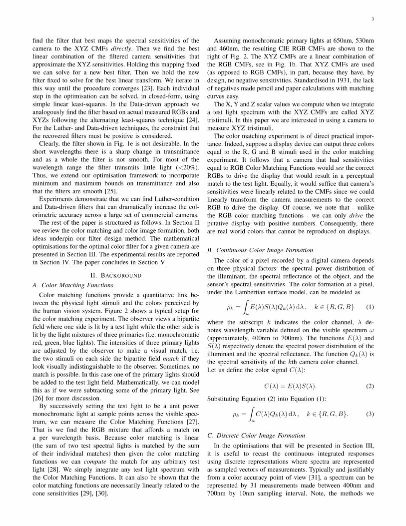
before the Luther-condition filter seeds the Data-driven op-timisation). Per camera, Figure 4 summarises the per cameramean and 95 percentile ∆E∗

ab performance.Grey bars in Figs. 4a and 4b show respectively the mean and

95 percentile error performance of native (un-filtered) colorcorrected RGBs for the 28 cameras. Respectively, the dashedgreen and solid red lines record the performance of the bestLuther-condition and Data-driven filters.

It is evident that the optimised filters support improvedcolor measurement for all 28 cameras and on average theperformance increment is significant. For many cameras theData-driven optimised filter delivers significantly better colormeasurement performance compared with using the Luther-condition optimised filter.

D. Smooth and Bounded Transmittance Filters

Both the Luther-condition and Data-driven filters absorbmuch of the available light (low transmittance values) and arefar from being smooth, e.g. see the derived Luther-conditionfilter in Fig. 1e. Here across much of the visible spectrum thefilter transmits little (below 20%) of the available light. Whena strongly light-absorptive filter is placed in front of a camerathen we need to either increase the exposure time (or widenthe aperture) or apply a higher ISO (which can increase theconspicuity of noise) to obtain an image with the same rangeof brightnesses (as when a filter is not used). Plus the filter inFig. 1e is not smooth it may be difficult to manufacture.

In this subsection we will constrain our optimisation so thatthe calculated filters are smooth and transmit, per wavelength,a minimum amount of incident light (here, 20%). We enforcesmoothness indirectly by assuming that our filters lie withinthe span of either a 6- or 8-dimensional Cosine basis.

Let us visualise the 20% bounded transmittance constraintusing the Canon 5D Mark II camera sensitivities and ourData-driven optimisation. First, we initialise the optimisation(Algorithm 2) using the uniform vector 1 (100% transmittance

10

(a) mean ∆E∗ab color error

(b) 95-percentile ∆E∗ab color error

Fig. 4. Mean (a) and 95-percentile (b) ∆E∗ab errors for 28 cameras. The grey-

bars show the color errors for NATive color correction. The dashed green lineswith black circles show the results by using the LUTHer-condition optimisedfilter. The results of the DATA-driven optimisation are plotted in solid redlines.

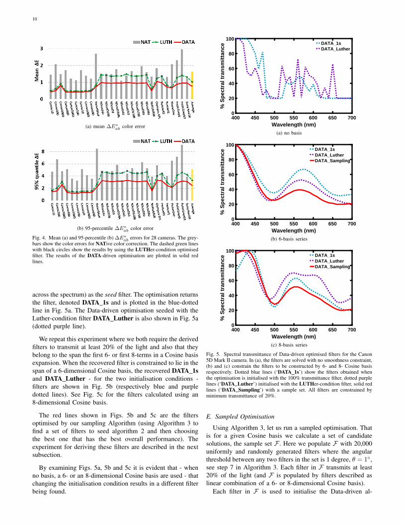
across the spectrum) as the seed filter. The optimisation returnsthe filter, denoted DATA 1s and is plotted in the blue-dottedline in Fig. 5a. The Data-driven optimisation seeded with theLuther-condition filter DATA Luther is also shown in Fig. 5a(dotted purple line).

We repeat this experiment where we both require the derivedfilters to transmit at least 20% of the light and also that theybelong to the span the first 6- or first 8-terms in a Cosine basisexpansion. When the recovered filter is constrained to lie in thespan of a 6-dimensional Cosine basis, the recovered DATA 1sand DATA Luther - for the two initialisation conditions -filters are shown in Fig. 5b (respectively blue and purpledotted lines). See Fig. 5c for the filters calculated using an8-dimensional Cosine basis.

The red lines shown in Figs. 5b and 5c are the filtersoptimised by our sampling Algorithm (using Algorithm 3 tofind a set of filters to seed algorithm 2 and then choosingthe best one that has the best overall performance). Theexperiment for deriving these filters are described in the nextsubsection.

By examining Figs. 5a, 5b and 5c it is evident that - whenno basis, a 6- or an 8-dimensional Cosine basis are used - thatchanging the initialisation condition results in a different filterbeing found.

400 450 500 550 600 650 700Wavelength (nm)

0

20

40

60

80

100

% S

pec

tral

tra

nsm

itta

nce

DATA_1sDATA_Luther

(a) no basis

400 450 500 550 600 650 700Wavelength (nm)

0

20

40

60

80

100

% S

pec

tral

tra

nsm

itta

nce

DATA_1sDATA_LutherDATA_Sampling

(b) 6-basis series

400 450 500 550 600 650 700Wavelength (nm)

0

20

40

60

80

100

% S

pec

tral

tra

nsm

itta

nce

DATA_1sDATA_LutherDATA_Sampling

(c) 8-basis series

Fig. 5. Spectral transmittance of Data-driven optimised filters for the Canon5D Mark II camera. In (a), the filters are solved with no smoothness constraint,(b) and (c) constrain the filters to be constructed by 6- and 8- Cosine basisrespectively. Dotted blue lines (‘DATA 1s’) show the filters obtained whenthe optimisation is initialised with the 100% transmittance filter, dotted purplelines (‘DATA Luther’) initialised with the LUTHer-condition filter, solid redlines (‘DATA Sampling’) with a sample set. All filters are constrained byminimum transmittance of 20%.

E. Sampled Optimisation

Using Algorithm 3, let us run a sampled optimisation. Thatis for a given Cosine basis we calculate a set of candidatesolutions, the sample set F . Here we populate F with 20,000uniformly and randomly generated filters where the angularthreshold between any two filters in the set is 1 degree, θ = 1◦,see step 7 in Algorithm 3. Each filter in F transmits at least20% of the light (and F is populated by filters described aslinear combination of a 6- or 8-dimensional Cosine basis).

Each filter in F is used to initialise the Data-driven al-

11

gorithm. That is we find 20,000 optimised filters. The colormeasurement performance of each filter in this solution set canbe calculated. Then we simply choose the filter that deliversthe best overall measurement performance. In Figs. 5b and 5cwe show the best sample-optimised filters (red lines) whichrespectively lie in the span of a 6- and 8-dimensional Cosinebasis (and transmit at least 20% of the light). Here ’best’ isdefined to be the filter that results in the smallest mean ∆E∗

ab

performance.Table II reports the ∆E∗

ab color error performance 1995reflectances and 102 lights [50] for the Canon 5D Mark II sen-sitivities. The row NAT reports the baseline color correctionresults when a per illuminant based linear correction matrixis applied while no filter is used (note that row 7 in Tables Iand row 1 in Table II are the same).

In Table II we report the correction performances in 3tranches. Rows 2 and 3 correspond to the two filters withoutusing Cosine basis as shown in Fig. 5a. Here we find thebest filters with only the 20% minimum transmittance bound.Rows, 4,5 and 6 report the performance when the 3 filtersshown in Fig. 5b are used, where the filter is additionallyconstrained to be in the span of the 6-dimensional Cosinebasis. Finally, when the filter is constrained to belong to an8-dimensional Cosine basis, the 3 derived filters lead to theerror statistics shown in rows 7 through 9.

Table I reported the color measurement performance of thefilters found using an unconstrained optimisation. Table II re-ports the color measurement results that are found when filtersare constrained to have a bounded transmittance (here at least20% of the light) and be smooth. Let us consider the boundedtransmittance first. Comparing row 9 of Table I to row 3 ofTable II we see that adding a lower transmittance bound returnsa filter that delivers poorer measurement performance (butstill much better compared with the native camera response).Additionally, requiring that our filters smooth on top of theminimum also yields relatively poorer performance comparedto the unconstrained filter optimisation.

However, with either the 6- and 8-dimensional Cosine basisconstraint we can find the best filter by seeding Algorithm 2with many possible filter initialisations (and then choosing thebest filter overall). Here, we find that comparable performanceis possible. Compare rows 6 and 9 of Table II to row 9 of TableI. It is remarkable how well a constrained filter can work: theperformance is ever so slightly worse than the unconstrainedoptimisation. But, the filter is much smoother and more likelyto be able to be manufactured.

F. Sampling vs OptimisationIt is worth reflecting on our sample-based optimisation.

Clearly, that sampling makes such a difference to the per-formance that our optimisation can deliver (for filtered colormeasurement) teaches us that the minimisation at hand hasmany local minima. By sampling we are effectively allowingour minimiser (Algorithm 2) to find many solutions and thenwe have the latitude to choose the (closer to) global minimum.Given we seed our optimisation with 20,000 filters we mightwonder whether we need to actually carry out the Data-drivenoptimisation.

TABLE II∆E∗

ab STATISTICS OF THE COLOR CORRECTED NATIVE CAMERA, THECOLOR CORRECTED CAMERA WITH THE DATA-DRIVEN OPTIMISED FILTERSOLUTIONS OBTAINED WHEN INITIALISED WITH UNIFORM VECTOR OF 1s,

Luther-CONDITION FILTER AND Sampling FILTER SET RESPECTIVELYUNDER DIFFERENT CONSTRAINTS FOR CANON 5D MARK II CAMERA

Mean Median 90% 95% 99% Max

NAT 1.72 1.03 3.68 5.12 12.94 28.39

minimum transmittance of 20%

DATA 1s 0.69 0.42 1.47 2.11 4.69 19.48

DATA Luther 0.58 0.38 1.36 1.80 2.77 5.75

6 cosine basis with 20% minimum transmittance

DATA 1s 0.81 0.49 1.80 2.54 5.21 18.85

DATA Luther 0.94 0.54 2.03 2.84 7.00 21.14

DATA Sampling 0.59 0.35 1.30 1.83 3.77 14.19

8 cosine basis with 20% minimum transmittance

DATA 1s 0.71 0.38 1.60 2.38 5.42 19.25

DATA Luther 0.62 0.38 1.41 2.01 3.47 9.52

DATA Sampling 0.45 0.25 1.02 1.41 3.10 10.63

In answering this question, first we remark that it is wellknown that as the dimension of a space increases it is moresparse. On the Cartesian plane if we have more than 360vectors (anchored at the origin) then the closest angulardistance to at least one vector’s nearest neighbours must beless than 1 degree. In 3-dimensions we can have thousandsof vectors where every vector is more than 1 degree from itsnearest neighbour.

For our 20,000 member sample set F we calculated theaverage angular distance for each element to its nearestneighbour in the set. When F is calculated subject to the6-dimensional Cosine basis constraint, the average nearest-neighbour distance was 2.6 degrees (with a maximum of 7)and for the 8-dimensional case it was 4.6 degrees (with amaximum of 10). Running the optimisation, Algorithm 2, witheach element in F , we effectively refine the initial guess. And,the refinement (difference between the starting and endpointfilter) is on the same order as the average nearest-neighbourdistance.

Significantly, running the optimisation - carrying out therefinement - results in a significant performance incrementcompared to using the only sample filters. That is we cannotuse the sampling strategy alone to find the best optimised filter.The importance of the refinement step will increase as a greaternumber of basis functions are used in the optimisation.

V. CONCLUSION

In this paper, we developed two algorithms that designtransmittance filters which, when placed in front of a camera,make the camera more colorimetric. Our first algorithm isdriven by the camera sensitivities themselves. It is well knownthat a camera that has sensitivities that are a linear transformfrom the XYZ color matching functions - the camera meets theLuther condition - can be used to measure color without error.Our first algorithm finds the filter that best satisfies the Luthercondition. A second algorithm that tackles color correction

12

for a given set of measured lights and surfaces, which we callData-driven filter optimisation, is also developed. Both Luther-and Data-driven Filters provide a step change in how well acamera can measure color.

Our default optimisation - though compellingly simple toformulate - deliver filters which are not smooth (difficultto make) and may also transmit very little light. Our op-timisations are reformulated to incorporate both smoothnessand a lower bound on how much light must be transmitted.Initially, when these constraints are adopted, the solved-forfilters work less well. However, experiments demonstrated thatour optimisations were highly dependent on the initialisationparameters, specifically the seed filter (initial guess) that drivesthe filter evolution. A simple sampling strategy - i.e. severallyrunning the optimisation for a set of judiciously chosen seedfilters - allows us to mitigate this problem. Significantly asmooth filter that transmits more than 20% of the light acrossthe visible spectrum delivers almost as good performance asa very non-transmittive and non-smooth filter (found via theunconstrained optimisations).

APPENDIXIMPLEMENTATION

For both Algorithms 1 and 2 presented in Section III thefilter and the color correction matrices can be found usingsimple least-squares regression. To remind the reader, givenA and B - m × n matrices of rank n where m ≥ n, thenthe least-squares regression M - an n × n matrix, mappingA to B (AM ≈ B) can be found in closed-form using theMoore-Penrose inverse [23]:

M = [ATA]−1ATB = A+B

A. Algorithm 1: ALS for the Luther-condition Optimisation

In step 4 of the algorithm, the optimal filter is found by find-ing scalars that maps each row of Qi−1 to the correspondingrow of X. The best scalar α mapping the vector v = [Qi−1

j ]T tow = [Xj ]

T (for the jth row of the data matrices) can be writtenin closed form using the Moore-Penrose inverse: α = vTw

vT v.

Similarly, in step 5, the Moore-Penrose inverse can beused for finding M . Denoting Q = diag(f i)Qi−1 thenM i = Q+X = [QTQ]−1QT X.

B. Algorithm 2: ALS for the Data-driven Optimisation

In step 4, each M ij can be solved directly using the

Moore-Penrose inverse. Denoting Q = CTj Q

i−1j then M i

j =

Q+CTk X = [QTQ]−1QTCT

k X.In step 5 of the Data-driven optimisation, the filter f is

embedded in the equation and so we cannot solve for it directlyas we could for the Luther-condition case.

To solve for the filter it is useful to vectorise the minimisa-tion. We recapitulate the minimisation statement of step 5:

minf

cnt∑j=1

‖ (CTj diag(f)QjMj − CT

k X) ‖2F (18)

The meaning of ‖ ‖2F is the Frobenius norm squared, i.e. thesum of all the argument terms squared. This Frobenius normis generally applied to matrices (as here) but can equallybe applied to vectors (where the vec() operator stacks thecolumns of a matrix on top of each other):

minf

cnt∑j=1

‖ vec(CTj diag(f)QjMj)− vec(CT

k X) ‖2F (19)

Now let us rewrite the diagonal filter matrix as a summationof each value in the diagonal, fi, multiplied with a singleentry matrix Di as diag(f) =

∑31i=1 fiDi. Here, Di is a 31×

31 matrix with a single non-zero entry at D(i, i) = 1. Bysubstituting this new filter representation into the first term ofthe minimisation in Equation (19), we obtain

vec(CTj diag(f)QjMj) =

31∑i=1

fi vec(CTj DiQjMj) (20)

Now let us denote a matrix Vj = [v1,j v2,j · · · v31,j ] whereits column represents vi,j = vec(CT

j DiQjMj), Equation (20)can be expressed more compactly as

vec(CTj diag(f)QjMj) = Vjf (21)

where f = [f1 f2 ... f31]T . Note that if Cj is a 31 × nmatrix then CT

j DiQjMj is an n× 3 matrix (where 3 denotesthe number of color channels) and thus vi,j is 3n × 1 whichmakes matrix Vj have size of 3n× 31.

Now we stack all Vj , j = 1, 2, .., cnt matrices (under cntdifferent lighting conditions) on top of each other making an(3n∗cnt)×31 matrix, V . Similarly we stack all cnt targetingXYZs on top of each other denoted as w = vec(CT

k X) whichhas the size of (3n∗cnt)×1. We remind the reader that k mightequal j. Or, k might denote a single privileged illuminant suchas CIE D65.

Now the minimisation in Equation (19) can be equivalentlyrewritten as:

minf‖ V f − w ‖2F (22)

The best f can be found in closed form using the Moore-Penrose inverse:

f = (V )+w = [V TV ]−1V Tw. (23)

C. Filter Constraints

Equation (23) solves for the 31-component f in one step.Suppose we write f = Bc. We constrain the filter to bedescribable by a linear basis (B is 31×m where 1 ≤ m ≤ 31).Additionally, the filter is restrained by a minimum fmin andmaximum fmax bounds on the transmittance. Then to solvefor the filter we find the coefficient vector c that minimises:

minc‖ V Bc− w ‖2F s.t. fmin ≤ Bc ≤ fmax (24)

Equation (24) where there is a quadratic objective functionand linear inequality constraints can be solved using quadraticprogramming [46].

13

ACKNOWLEDGMENT

This work was supported by EPSRC under GrantEP/S028730. The authors would also like to thank Dr. JavierVazquez-Corral for his insightful comments.

REFERENCES

[1] R. W. G. Hunt and M. R. Pointer, Measuring colour, 4th ed. JohnWiley & Sons, 2011.

[2] B. A. Wandell, Foundations of vision. Sinauer Associates, 1995.[3] N. Ohta and A. Robertson, Colorimetry: fundamentals and applications.

John Wiley & Sons, 2006.[4] H. E. Ives, “The transformation of color-mixture equations from one

system to another,” Journal of the Franklin Institute, vol. 180, no. 6, pp.673–701, 1915.

[5] R. Luther, “Aus dem gebiet der farbreizmetrik,” Zeitschrift TechnischePhysik, vol. 8, pp. 540–558, 1927.

[6] J. P. S. Parkkinen, J. Hallikainen, and T. Jaaskelainen, “Characteristicspectra of munsell colors,” Journal of the Optical Society of America A,vol. 6, no. 2, pp. 318–322, 1989.

[7] M. J. Vrhel, R. Gershon, and L. S. Iwan, “Measurement and analysisof object reflectance spectra,” Color Research & Application, vol. 19,no. 1, pp. 4–9, 1994.

[8] C.-C. Chiao, T. W. Cronin, and D. Osorio, “Color signals in naturalscenes: characteristics of reflectance spectra and effects of naturalilluminants,” Journal of the Optical Society of America A, vol. 17, no. 2,pp. 218–224, 2000.

[9] L. T. Maloney, “Evaluation of linear models of surface spectral re-flectance with small numbers of parameters,” Journal of the OpticalSociety of America A, vol. 3, no. 10, pp. 1673–1683, 1986.

[10] D. H. Marimont and B. A. Wandell, “Linear models of surface andilluminant spectra,” Journal of the Optical Society of America A, vol. 9,no. 11, pp. 1905–1913, 1992.

[11] P. R. Boyce, Human factors in lighting, 2nd ed. Talor & Francis, 2003.[12] M. S. Drew and B. V. Funt, “Natural metamers,” CVGIP: Image

Understanding, vol. 56, no. 2, pp. 139–151, 1992.[13] G. Hong, M. R. Luo, and P. A. Rhodes, “A study of digital camera

colorimetric characterization based on polynomial modeling,” ColorResearch & Application, vol. 26, no. 1, pp. 76–84, 2001.

[14] G. D. Finlayson, M. Mackiewicz, and A. Hurlbert, “Color correctionusing root-polynomial regression,” IEEE Transactions on Image Pro-cessing, vol. 24, no. 5, pp. 1460–1470, 2015.

[15] P.-C. Hung, “Colorimetric calibration in electronic imaging devicesusing a look-up-table model and interpolations,” Journal of ElectronicImaging, vol. 2, no. 1, pp. 53–62, 1993.

[16] C. F. Andersen and D. Connah, “Weighted constrained hue-plane pre-serving camera characterization,” IEEE Transactions on Image Process-ing, vol. 25, no. 9, pp. 4329–4339, 2016.

[17] G. J. Klinker, S. A. Shafer, and T. Kanade, “A physical approach tocolor image understanding,” International Journal of Computer Vision,vol. 4, no. 1, pp. 7–38, 1990.

[18] M. Mackiewicz, C. F. Andersen, and G. D. Finlayson, “Method for hueplane preserving color correction,” Journal of the Optical Society ofAmerica A, vol. 33, no. 11, pp. 2166–2177, 2016.

[19] T. Zhang and G. H. Golub, “Rank-one approximation to high ordertensors,” SIAM Journal on Matrix Analysis and Applications, vol. 23,no. 2, pp. 534–550, 2001.

[20] G. D. Finlayson, M. M. Darrodi, and M. Mackiewicz, “The alternatingleast squares technique for nonuniform intensity color correction,” ColorResearch & Application, vol. 40, no. 3, pp. 232–242, 2015.

[21] G. D. Finlayson, H. G. Gong, and R. B. Fisher, “Color homography:Theory and applications,” IEEE Transactions on Pattern Analysis andMachine Intelligence, vol. 41, pp. 20–33, 2019.

[22] G. D. Finlayson, Y. Zhu, and H. Gong, “Using a simple colour pre-filterto make cameras more colorimetric,” in Color and Imaging Conference,vol. 2018, no. 1. Society for Imaging Science and Technology, 2018,pp. 182–186.

[23] G. H. Golub and C. F. Van Loan, Matrix computations, 3rd ed. JohnsHopkins University Press, 1996.

[24] G. D. Finlayson and Y. Zhu, “Finding a colour filter to make acamera colorimetric by optimisation,” in International Workshop onComputational Color Imaging. Springer, 2019, pp. 53–62.

[25] Y. Zhu and G. Finlayson, “An improved optimization method for findinga color filter to make a camera more colorimetric,” in Electronic Imaging2020. Society for Imaging Science and Technology, 2020.

[26] J. Guild, “The colorimetric properties of the spectrum,” PhilosophicalTransactions of the Royal Society of London. Series A, ContainingPapers of a Mathematical or Physical Character, vol. 230, no. 681-693, pp. 149–187, 1931.

[27] G. Wyszecki and W. S. Stiles, Color science: Concepts and Methods,Quantitative Data and Formulae, 2nd ed. Wiley New York, 1982.

[28] D. H. Krantz, “Color measurement and color theory: I. representationtheorem for grassmann structures,” Journal of Mathematical Psychology,vol. 12, no. 3, pp. 283–303, 1975.

[29] P. DeMarco, J. Pokorny, and V. C. Smith, “Full-spectrum cone sensitivityfunctions for x-chromosome-linked anomalous trichromats,” Journal ofthe Optical Society of America A, vol. 9, no. 9, pp. 1465–1476, 1992.

[30] A. Stockman and L. T. Sharpe, “The spectral sensitivities of the middle-and long-wavelength-sensitive cones derived from measurements inobservers of known genotype,” Vision research, vol. 40, no. 13, pp.1711–1737, 2000.

[31] B. Smith, C. Spiekermann, and R. Sember, “Numerical methods for col-orimetric calculations: sampling density requirements,” Color Research& Application, vol. 17, no. 6, pp. 394–401, 1992.

[32] B. K. P. Horn, “Exact reproduction of colored images,” Computer Vision,Graphics, and Image Processing, vol. 26, no. 2, pp. 135 – 167, 1984.

[33] P. L. Vora and H. J. Trussell, “Mathematical methods for the design ofcolor scanning filters,” IEEE Transactions on Image Processing, vol. 6,no. 2, pp. 312–320, 1997.

[34] M. J. Vrhel and H. J. Trussell, “Filter considerations in color correction,”IEEE Transactions on Image Processing, vol. 3, no. 2, pp. 147–161,1994.

[35] M. J. Vrhel and H. J. Trussell, “Optimal color filters in the presenceof noise,” IEEE Transactions on Image Processing, vol. 4, no. 6, pp.814–823, 1995.

[36] M. Wolski, C. Bouman, J. P. Allebach, and E. Walowit, “Optimizationof sensor response functions for colorimetry of reflective and emissiveobjects,” IEEE Transactions on Image Processing, vol. 5, no. 3, pp.507–517, 1996.

[37] P. L. Vora and H. J. Trussell, “Mathematical methods for the analysis ofcolor scanning filters,” IEEE Transactions on Image Processing, vol. 6,no. 2, pp. 321–327, 1997.

[38] G. Sharma and H. J. Trussell, “Digital color imaging,” IEEE transactionson Image Processing, vol. 6, no. 7, pp. 901–932, 1997.

[39] J. E. Farrell and B. A. Wandell, “Method and apparatus for identifyingthe color of an image,” Dec. 26, 1995, U.S. Patent 5479524.

[40] J. Y. Hardeberg, Acquisition and reproduction of color images: colori-metric and multispectral approaches. Universal-Publishers, 2001.

[41] D. Connah, S. Westland, and M. Thomson, “Recovering spectral infor-mation using digital camera systems,” Coloration Technology, vol. 117,no. 6, pp. 309–312, 2001.

[42] J. L. Nieves, E. M. Valero, S. M. Nascimento, J. Hernandez-Andres,and J. Romero, “Multispectral synthesis of daylight using a commercialdigital CCD camera,” Applied Optics, vol. 44, no. 27, pp. 5696–5703,2005.

[43] D.-Y. Ng and J. P. Allebach, “A subspace matching color filter designmethodology for a multispectral imaging system,” IEEE Transactionson Image Processing, vol. 15, no. 9, pp. 2631–2643, 2006.

[44] E. M. Valero, J. L. Nieves, S. M. Nascimento, K. Amano, and D. H.Foster, “Recovering spectral data from natural scenes with an RGBdigital camera and colored filters,” Color Research & Application,vol. 32, no. 5, pp. 352–360, 2007.

[45] G. Sharma and R. Bala, Digital color imaging handbook. CRC press,2002.

[46] D. G. Luenberger and Y. Ye, Linear and nonlinear programming, 4th ed.Springer, 2015.

[47] G. Strang, “The discrete cosine transform,” SIAM review, vol. 41, no. 1,pp. 135–147, 1999.

[48] P. L. Vora and H. J. Trussell, “Measure of goodness of a set of color-scanning filters,” Journal of the Optical Society of America A, vol. 10,no. 7, pp. 1499–1508, 1993.

[49] J. Jiang, D. Liu, J. Gu, and S. Susstrunk, “What is the space of spectralsensitivity functions for digital color cameras?” in 2013 IEEE Workshopon Applications of Computer Vision (WACV). IEEE, 2013, pp. 168–179.

[50] K. Barnard, L. Martin, B. Funt, and A. Coath, “A data set for colorresearch,” Color Research & Application, vol. 27, no. 3, pp. 147–151,2002.