Designing and Testing Precise Time-Distribution Systems

Designing and Testing Precise Time-Distribution Systems

Edmund O. Schweitzer, III, David Whitehead, Ken Fodero, and Shankar Achanta Schweitzer Engineering Laboratories, Inc.

Published in Line Current Differential Protection: A Collection of

Technical Papers Representing Modern Solutions, 2014

Previously presented at the 4th Annual Protection, Automation and Control World Conference, June 2013,

and 16th Annual Georgia Tech Fault and Disturbance Analysis Conference, May 2013

Originally presented at the 39th Annual Western Protective Relay Conference, October 2012

1

Designing and Testing Precise Time-Distribution Systems

Edmund O. Schweitzer, III, David Whitehead, Ken Fodero, and Shankar Achanta, Schweitzer Engineering Laboratories, Inc.

Abstract—Modern power systems rely on accurate time for protection, monitoring, and control. The availability of high-accuracy time (less than 1 microsecond) is now required for many applications deployed, or that will be deployed, in modern substation designs, including synchrophasors and IEC 61850 Sampled Value messaging.

The conventional method of high-accuracy time distribution is provided by individual or multiple Global Positioning System (GPS) clocks collocated at each substation at which high-accuracy time service is required. New methods of precise time distribution over wide areas are being implemented via terrestrial private fiber-optic systems such as synchronous optical network (SONET) or Ethernet. Advantages to these systems are:

Fewer clock sources are required.

Time signals distributed over a fiber-optic communications system are immune to external radio interference.

This paper reviews the design choices available in the development of robust precise time-distribution systems, analyzes the various failure scenarios of wide-area network time systems, and develops test methods to measure time-distribution performance. Finally, the paper discusses methods to minimize or eliminate precise time failures in power system applications requiring precise time.

I. INTRODUCTION

The availability of accurate Global Positioning System-based (GPS-based) time has become almost commonplace in substations and control facilities. Advancements in GPS receiver technology have brought the price of these devices down to a point where they are easily justified for wide-scale deployment. Additionally, regulations now require the use of accurate time distribution across power transmission networks to aid in the evaluation of system disturbances.

Typical time-distribution systems used in power system applications consist of a GPS receiver with one or more IRIG-B outputs [1]. The IRIG-B outputs are then directly connected to intelligent electronic devices (IEDs) or are daisy-chained from one IED to another.

Fig. 1 is a typical IRIG-B distribution diagram for a high-accuracy (less than 1 microsecond) time-distribution network in a substation [2].

Fig. 1. Simple time-distribution network.

Ensuring that the GPS clock and IEDs are communicating has typically been easy to determine. The connections are essentially point to point, the GPS receivers provide status indications of time-quality status, and IEDs typically provide GPS time reception status. Traditionally, the time accuracy in these installations is essentially that of the GPS clock. The cables and any downstream devices used to distribute time from one input to many IEDs are the only devices in the network that add latency to the distributed time signals. These distribution delays total in the range of nanoseconds. Table I provides the cable latencies that can be expected and, in most cases, are well within the strictest requirement of 1 microsecond required by synchrophasor or other similar protocols. When the time is only used for time-stamping events, 1 millisecond is sufficient.

TABLE I PROPAGATION DELAY MEASUREMENTS

Cable Type Propagation Delay

Twisted Copper 1.90 ns/ft

Coaxial 1.85 ns/ft

Fiber 1.67 ns/ft

Many IEDs used in power system applications have dedicated inputs specifically designed to accept the high-accuracy, demodulated, IRIG-B time format. These IEDs incorporate electronics that process the time data and apply the data directly to the real-time clock of the device.

In the past, there was no need for additional specialized testing of these time systems. As long as the GPS clock outputs and the IED time inputs were operating within their specified ranges, the overall time systems were within the specified time accuracies.

II. WIDE-AREA TIME-DISTRIBUTION NETWORKS

Traditional time-distribution systems are generally found to be reliable, operating with a mean time between failures (MTBF) of 300 years or greater. This means that in a population of 300 clocks, a failure of one per year can be experienced. Applications include time-stamped sequence of events (SOE) reports and demand metering. However, with the broad deployment of synchrophasors and emerging technologies such as using IEC 61850 Sampled Value messaging, accurate time, and robust time in wide-area networks, distribution systems are now critical. Further, traditional GPS-based time-distribution systems do suffer

2

from a few issues. For example, the satellite receiver is a single point of failure. The GPS system is controlled by the United States government, which can, and has, affected the accuracy of the system; and the GPS system is subject to the influences of the sun (solar flares) and potentially satellite signal spoofing. Other failures include faults in the antenna system cables and hardware-related failures.

Wide-area communications systems can now be used to also distribute time. There are two types of wide-area time-distribution schemes, also known as terrestrial time-distribution systems (TTDSs) beginning to be deployed. One is based on time-division multiplexing (TDM) techniques, and the other is an Ethernet-based scheme. These systems use multiple time sources (e.g., GPS and precision-time references), combine them, and then produce a best-estimate time signal. The advantage to this sort of system is that it addresses the issues of the single satellite clock system. Further, even if all external time sources are lost, these systems have the ability to provide a relative time throughout the time-distribution system (i.e., the time being distributed may not be correlated with absolute time, but all nodes within the system are using the same time).

Fig. 2 is an example diagram of an IEEE 1588 implementation that uses the Ethernet network to distribute time. Through the use of specialized Ethernet switches, time is distributed from redundant master clocks in the network to provide high-accuracy time to remote locations.

Fig. 2. Time-distribution hierarchy using the IEEE 1588 standard [3].

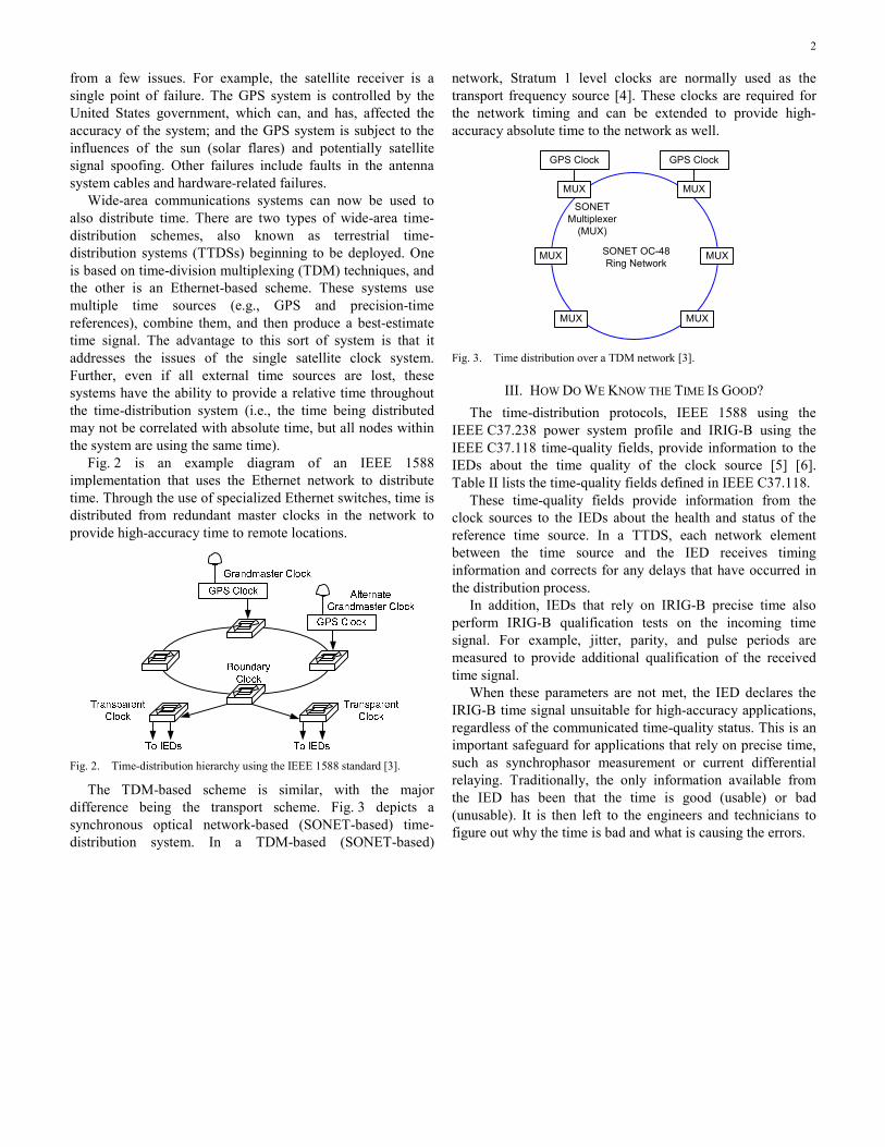
The TDM-based scheme is similar, with the major difference being the transport scheme. Fig. 3 depicts a synchronous optical network-based (SONET-based) time-distribution system. In a TDM-based (SONET-based)

network, Stratum 1 level clocks are normally used as the transport frequency source [4]. These clocks are required for the network timing and can be extended to provide high-accuracy absolute time to the network as well.

GPS Clock GPS Clock

SONET OC-48 Ring Network

SONET Multiplexer

(MUX)

MUX MUX

MUX MUX

MUX MUX

Fig. 3. Time distribution over a TDM network [3].

III. HOW DO WE KNOW THE TIME IS GOOD?

The time-distribution protocols, IEEE 1588 using the IEEE C37.238 power system profile and IRIG-B using the IEEE C37.118 time-quality fields, provide information to the IEDs about the time quality of the clock source [5] [6]. Table II lists the time-quality fields defined in IEEE C37.118.

These time-quality fields provide information from the clock sources to the IEDs about the health and status of the reference time source. In a TTDS, each network element between the time source and the IED receives timing information and corrects for any delays that have occurred in the distribution process.

In addition, IEDs that rely on IRIG-B precise time also perform IRIG-B qualification tests on the incoming time signal. For example, jitter, parity, and pulse periods are measured to provide additional qualification of the received time signal.

When these parameters are not met, the IED declares the IRIG-B time signal unsuitable for high-accuracy applications, regardless of the communicated time-quality status. This is an important safeguard for applications that rely on precise time, such as synchrophasor measurement or current differential relaying. Traditionally, the only information available from the IED has been that the time is good (usable) or bad (unusable). It is then left to the engineers and technicians to figure out why the time is bad and what is causing the errors.

3

TABLE II TIME-ACCURACY LEVELS OF IEEE C37.118

IRIG-B Position

ID

Control Bit

Number Designation Explanation

P 50 1 Year, BCD 1

Last two digits of year in binary code decimal (BCD)

P 51 2 Year, BCD 2

P 52 3 Year, BCD 4

P 53 4 Year, BCD 8

P 54 5 Not used Unassigned

P 55 6 Year, BCD 10

Last two digits of year in BCD

P 56 7 Year, BCD 20

P 57 8 Year, BCD 40

P 58 9 Year, BCD 80

P 59 – P6 Position identifier #6

P 60 10 Leap second

pending Becomes 1 up to 59 seconds

before leap second insert

P 61 11 Leap second 0 = add leap second,

1 = delete leap second

P 62 12 Daylight saving

pending

Becomes 1 up to 59 seconds before daylight-saving time

(DST) change

P 63 13 DST Becomes 1 during DST

P 64 14 Time offset

sign Time offset sign: 0 = +, 1 = –

P 65 15 Time offset:

Binary 1 Offset from coded IRIG-B

time to Coordinated Universal Time (UTC); IRIG-B coded

time plus time offset (including sign) equals UTC time at all times (offset will

change during DST)


Binary 2


Binary 4


Binary 8



0.5 hours 0 = none, 1 = additional

0.5-hour time offset; 4-bit code representing

approximate clock time error;0000 = clock locked, maximum accuracy; 1111 = clock failed,

data unreliable

P 71 20 Time quality




P 75 24 Parity Parity on all preceding

data bits





Newer IEDs are now providing both analog and digital measurement data to aid in the troubleshooting of high-accuracy time inputs. Fig. 4 demonstrates event report information collected by an IED regarding the accuracy of the time signal at the BNC time input. An IRIG-B signal corruption device was used to add jitter to the IRIG-B signal while representing high accuracy in the time-quality bit fields. The scale for the analog data is in microseconds. The IED uses a very stable internal clock that is phase-locked to the received IRIG-B time signal. The time difference between when the IRIG-B signal is received and when the IED phase-locked clock expects the signal is measured. Any time difference measured between these two sources is considered time error. To measure jitter on the incoming clock signal, the IED runs a counter with 25-nanosecond increments, the number of counts between pulses is compared with the previous count, and any difference greater than 500 nanoseconds between measurements is considered excessive. In Fig. 4, the jitter measured by the IED is excessive and results in the TSOK (time signal okay) bit not being asserted, which means the IED is not using this time source. The 1-pulse-per-second (PPS) jitter signal represents the time difference measurement, and the 10-millisecond jitter signal represents the jitter measurement.

Fig. 4. Bad-quality IRIG-B measurements in an IED.

Fig. 5 is a data capture of a good IRIG-B input signal. The TSOK bit in this capture remains asserted, indicating the time input signal is within the jitter parameters and is acceptable for use in applications requiring high accuracy.

Fig. 5. Good-quality IRIG-B measurements in an IED.

4

IV. HOW CAN WE TEST AND VERIFY TIME QUALITY?

At the time we wrote this paper, Ethernet devices providing time distribution using IEEE 1588 with the IEEE C37.238 power system profile were not widely available, and system-level testing capabilities were very limited. As a result, time network testing and analysis will be the research effort of white paper. The TTDS testing and analysis in this paper were performed on a TDM-based time-distribution network. However, the testing methodologies outlined and performed in the following sections are applicable to both TTDS schemes.

A. Test Equipment

The test equipment used was the TimeSpy, which is manufactured by Brandywine Communications and designed to measure the time accuracy of a wide range of inputs against an internal precision GPS-disciplined oscillator. The tester measures the time error at the point of use for systems where time is distributed over large distances.

The test equipment accuracy is rated 25 nanoseconds at 1 sigma against an internal GPS reference clock with a measurement resolution of 0.2 nanoseconds. The test equipment has the ability to measure a PPS time signal input and compare the measured input against the internal reference clock. The data provided are the time offset between the test input and its internal GPS reference clock. The sample interval is also programmable. For the data presented in this paper, a sample interval of 1 second was used.

B. Test Network

The tests were performed on a 27-node, dual-ring SONET system. The test system had three nodes with GPS time sources activated. All test measurements were taken at Node B, which is also the location of the GPS primary signal source for the network. The primary source is determined through initial setup and programming of the system. Fig. 6 displays the topology of the network that was tested, including the locations of the GPS time sources.

Fig. 6. The network topology used for the testing.

The Node B location was selected as the test location for two reasons: it was the location of the master time source in the network, and it had access to a GPS antenna, which is a required input for the test set. Collocating the test set with the Node B unit also allowed the use of an antenna splitter at that location to feed the test network and test equipment. This was important because the antenna was located on the roof of the test facility and the antenna cable length was eliminated as a source of error. Fig. 7 is an illustration of the test set connections.

Fig. 7. Test equipment connections at the Node B location.

V. SYSTEM TESTING

The selected test scenarios reflect real-world conditions that have an effect on the ability of the TTDS to distribute accurate time. The tests selected are summarized as follows:

Establish baseline TTDS. Measure time accuracy across the network. Establish baseline data at a node that is collocated

with a GPS source. Establish baseline data at a node on the ring

farthest from a GPS source. Complete external time-source failure. System forced

to run on internal time references only. Measure and plot the drift (2 to 3 hours). Connect an antenna and plot the recovery.

A. System Baseline Testing and Results

The first test conducted was to determine the system performance under ideal conditions. The data produced were then used as the baseline for comparison against all other test results. For all tests, unless noted otherwise, the test equipment was set up to record 10,000 measurements at a 1-second interval (2.78 hours of data).

The baseline test setup was exactly as shown in Fig. 6, with all three GPS sources active in the test network.

The graph in Fig. 8 shows the 10,000 samples across the X axis and the time offset of the measurement compared with the time standard of the test equipment on the Y axis. In the baseline chart, we can see that the measured time difference averaged about a 40-nanosecond offset with excursions as high as 75 nanoseconds. The time accuracy requirements for most IEDs in power system applications (synchrophasors and so on) is 1 microsecond (±500 nanoseconds), so these data confirm that the system is more than sufficient for these applications.

5

Fig. 8. Baseline system performance graph.

B. GPS Source 10 Nodes Away

This measurement was performed again with the only GPS source in the network located 10 nodes away from the Node B terminal (Node I). The graph in Fig. 9 shows that the time difference from the reference clock averages 60 nanoseconds, with the excursions ranging from 7 to 107 nanoseconds. Although we see a shift in the offset from the reference clock, the system is still well within the stated accuracy of ±500 nanoseconds.

0

20

40

60

80

100

120

1,000 2,000 3,000 4,000 5,000 6,000 7,000 8,000 9,000Samples

10,000

Fig. 9. Remote GPS source system performance graph.

C. Remove All GPS Sources and Measure System Drift

This test was run with all GPS sources removed from the TTDS. The test network was used to record the time drift off of the internal clock of the system over time. Fifteen thousand samples were collected, resulting in just over 4 hours of data. As seen in Fig. 10, the drift is linear and constant. This curve reflects the stability of the TTDS internal oscillator. This test provides an excellent way to determine the quality of the internal clock accuracy of the system. Fig. 10 shows that over the 4-hour period without a GPS input on the system, the time accuracy only drifted 350 microseconds. Although this is out of specification for the absolute ±1-microsecond rating, this time output is still suitable for all applications that only require absolute 1-millisecond accuracy. Note that the system will continue to drift at this rate without a GPS input—after

about 9 hours, the time output will not be usable for systems that require absolute 1-millisecond accuracy. One very important note about this system is that even if the TTDS network time has drifted away from absolute time, all IEDs connected to the TTDS will have the same relative time to better than ±500 nanoseconds. However, the time-quality bits will represent the accuracy referenced to the GPS system, not the time island.

Se

0

150,000

200,000

250,000

300,000

350,000

400,000

100,000

50,000

2,000 4,000 6,000 8,000 10,000 12,000 14,000Samples

Fig. 10. System time drift without a GPS input source.

D. Reapply a GPS Source and Measure System Recovery

The antenna at Node B was disconnected for 24 hours while the system continued to operate using the GPS source from Node I. Next, the Node I GPS antenna cable was removed, causing a loss of valid GPS time to the system. Next, the antenna cable was reconnected at Node B. This ensured that the almanac information in the GPS receiver at Node B was stale. Fig. 11 shows the system recovery, including reacquisition of the GPS system. Node I was not reconnected for this test.

As shown, it takes about a minute for the GPS receiver to reacquire lock and about another minute for the time output to stabilize. It is interesting that the system is performing to within the ±1-microsecond specified output within about 100 seconds.

Fig. 11. System time recovery with GPS reacquisition.

6

The test was rerun. This time, the system was allowed to drift away from absolute GPS by about 1.5 milliseconds, and then a GPS signal was applied at Node I. Fig. 12 shows the almost instantaneous return to ±1-microsecond accuracy. There are currently two schools of thought on time recovery. One is that the system should return as quickly as possible and that IEDs should use the time-quality information to determine when to use the time signal input, and the other is to have a settable slew rate at which the time signal will recover. There are no standards or specifications at this time on system recovery from a loss of GPS. The reason for the quick return to absolute time in the TTDS is that when the GPS was turned off through the management settings, only the output was disabled and the GPS receiver was still operational and tracking satellites.

Fig. 12. System time recovery with GPS enabled.

VI. ADDITIONAL TESTING

The correct handling of leap seconds has always been a challenge for all time-distribution systems. When the time is used for an SOE report or oscillography, the possibility of a 1-second discrepancy between time domains for a short period every few years is mostly an inconvenience. However, for relaying and control systems that rely on high-accuracy time as part of their data sampling and decision process, a 1-second difference can have significant implications for synchrophasor applications, SOE report time stamps, and so on. There is no test equipment to verify that a product is providing time correctly during a leap second event; users rely on the design of the equipment to correctly handle these events.

A leap second was added on June 30, 2012, which allowed the observation of how various time sources handle such an event. There are few test devices available to test leap second events and none that can test multiple products simultaneously during a leap second event. The following test bed was created to record up to seven sources and two Internet sources simultaneously.

Test hardware and software were created to decode and display various fields in the IRIG-B message. A computer was used to display the data as they transitioned through the leap second event. Fig. 13 is a screen capture of the test recording. In this capture, the decoded values of six IRIG-B, one Precision Time Protocol (PTP), and two Internet clocks are simultaneously displayed.

Fig. 13. Screen capture from the leap second test station.

7

TABLE III RECORDED IRIG-B TIME VALUES DURING THE LEAP SECOND EVENT

Official United

States Time

GMT (Standard

Time)

Product A Product B Product C Product D

Standard Local Standard Local

1 16:59:59 11:59:59 23:59:58 16:59:58 23:59:58 16:59:58 15:59:58 23:59:59

2 16:59:60 0:00:00 23:59:59 16:59:59 23:59:59 16:59:59 15:59:59 00:00:00

3 17:00:00 0:00:01 23:59:60 16:59:60 00:00:60 16:59:60 16:00:00 00:00:01

4 17:00:01 0:00:02 00:00:00 17:00:00 00:00:00 17:00:00 16:00:01 00:00:02

5 17:00:02 0:00:03 00:00:01 17:00:01 00:00:01 17:00:01 16:00:02 00:00:03

Table III lists the decoded time values for eight of the nine

systems monitored during the event. The output of the PTP system is not used in Table III

because the time output was in straight binary seconds (SBS) format. The eight time captures in Table III include two pairs of the same products tested with standard and local time formats. As demonstrated in Table III, not all of the products handled the leap second event correctly, and there were some discrepancies with those that did. Leap seconds are a challenge to more than the equipment providing time. This leap second event caused several Internet systems to fail as well. There were several Java and Linux® server applications that crashed because of the unexpected extra second.

When testing leap seconds, remember it is just as important to test the applications running on the IEDs as to test how the time-distribution systems handle the events.

VII. CONCLUSION

Time-distribution systems have been implemented and in service for the past decade. Early implementations of these systems simply provided a time source for event recorders and IEDs. Now, with inexpensive high-accuracy time sources commonly available and the evolution of high-accuracy time available directly from the communications network, advanced protection and control schemes are including time in the measurement process. A TTDS system provides advantages over a traditional GPS-based system that includes redundancy, resulting in higher reliability and a means to keep all TTDS-connected devices time-synchronized to within a microsecond.

With the advent of inexpensive test equipment, network accuracy can be verified at any point within a time-distribution system.

With many applications relying on precise time, modern IEDs must be capable of measuring incoming time signal quality and identifying jitter and noise introduced in the transmission of these time signals that may have an effect on the time accuracy.

When time sources are in disagreement due to mishandling of leap second events or improper daylight-saving time settings, the time is still good in regard to the clock accuracy reported by the clock. Most IEDs are not aware of these events and have no way to validate that these events have occurred. The use of UTC time avoids these conditions and should be considered as the time reference for any wide-area time system.

Typically, we take for granted that the time-distribution system is working properly. We also rely on the clock sources to indicate when the accuracy is degraded from the expected value. As time systems become more widely used and relied upon for protection and control decisions, consideration should be given to how to validate new wide-area time-distribution schemes when installed and when the communications network topology is changed for systems that deliver these time signals.

VIII. REFERENCES [1] IRIG Standard 200-04, IRIG Serial Time Code Formats, Range

Commanders Council Telecommunications and Timing Group, September 2004.

[2] K. Behrendt and K. Fodero, “The Perfect Time: An Examination of Time-Synchronization Techniques,” proceedings of the 60th Annual Georgia Tech Protective Relaying Conference, Atlanta, GA, May 2006.

[3] K. Fodero, C. Huntley, and D. Whitehead, “Secure, Wide-Area Time Synchronization,” proceedings of the 12th Annual Western Power Delivery Automation Conference, Spokane, WA, April 2010.

[4] E. O. Schweitzer, III, D. Whitehead, S. Achanta, and V. Skendzic, “Implementing Robust Time Solutions for Modern Power Systems,” proceedings of the 14th Annual Western Power Delivery Automation Conference, Spokane, WA, March 2012.

[5] IEEE Standard 1588-2008, Standard for a Precision Clock Synchronization Protocol for Networked Measurement and Control Systems, July 2008.

[6] IEEE Standard C37.238-2011, IEEE Standard Profile for Use of IEEE 1588 Precision Time Protocol (PTP) in Power Systems.

8

IX. BIOGRAPHIES Dr. Edmund O. Schweitzer, III is recognized as a pioneer in digital protection and holds the grade of Fellow of the IEEE, a title bestowed on less than one percent of IEEE members. In 2002, he was elected a member of the National Academy of Engineering. He is the recipient of the Graduate Alumni Achievement Award from Washington State University and the Purdue University Outstanding Electrical and Computer Engineer Award. In September 2005, he was awarded an honorary doctorate from Universidad Autónoma de Nuevo León in Monterrey, Mexico, for his contribution to the development of electric power systems worldwide. He has written dozens of technical papers in the areas of digital relay design and reliability and holds more than 30 patents pertaining to electric power system protection, metering, monitoring, and control. Dr. Schweitzer received his Bachelor’s and Master’s degrees in electrical engineering from Purdue University and his Ph.D. from Washington State University. He served on the electrical engineering faculties of Ohio University and Washington State University, and in 1982, he founded Schweitzer Engineering Laboratories, Inc. (SEL) to develop and manufacture digital protective relays and related products and services. Today, SEL is an employee-owned company that serves the electric power industry worldwide and is certified to the international quality standard ISO-9001. SEL equipment is in service at voltages from 5 kV through 500 kV to protect feeders, motors, transformers, capacitor banks, transmission lines, and other power apparatus.

David Whitehead, P.E., is the vice president of research and development at Schweitzer Engineering Laboratories, Inc. (SEL). Prior to joining SEL, he worked for General Dynamics Electric Boat Division as a combat systems engineer. He received his BSEE from Washington State University in 1989 and his MSEE from Rensselaer Polytechnic Institute in 1994 and is pursuing his Ph.D. at the University of Idaho. He is a registered professional engineer in Washington and Maryland and a senior member of the IEEE. Mr. Whitehead holds seven patents with several other patents pending. He has worked at SEL since 1994 as a hardware engineer, research engineer, and a chief engineer/assistant director and has been responsible for the design of advanced hardware, embedded firmware, and PC software.

Ken Fodero is currently a research and development manager for the time and communications product lines at Schweitzer Engineering Laboratories, Inc. (SEL) in Pullman, Washington. Before coming to SEL, he was a product manager at Pulsar Technology for four years in Coral Springs, Florida. Prior to Pulsar Technology, Mr. Fodero worked at RFL Electronics for 15 years, and his last position there was Director of Product Planning.

Shankar Achanta received his MS in electrical engineering from Arizona State University in 2002. He joined Schweitzer Engineering Laboratories, Inc. (SEL) in 2002 as a hardware engineer, developing electronics for communications devices, data acquisition circuits, and switch mode power supplies. Mr. Achanta received a patent for a self-calibrating time-code generator while working at SEL. He presently holds the position of development manager for the precise time and communications group at SEL.

© 2012 by Schweitzer Engineering Laboratories, Inc. All rights reserved.

20120914 • TP6573-01

Designing and Testing Precise Time-Distribution Systems

Documents

Transcript of Designing and Testing Precise Time-Distribution Systems