Designing and Accelerating a Generic FFT Library in Futhark
51
FACULTY OF SCIENCE UNIVERSITY OF COPENHAGEN BSc Thesis in Computer Science Mette Marie Kowalski <bpr314> Designing and Accelerating a Generic FFT Library in Futhark Supervisor: Cosmin Eugen Oancea June 12, 2018
Transcript of Designing and Accelerating a Generic FFT Library in Futhark
F A C U L T Y O F S C I E N C E U N I V E R S I T Y O F C O P E N H A G E N
BSc Thesis in Computer ScienceMette Marie Kowalski <bpr314>
Designing and Acceleratinga Generic FFT Library in Futhark
Supervisor: Cosmin Eugen Oancea
June 12, 2018
Abstract
The Fast Fourier Transform (FFT) is a computationally intensive operation used ina variety of fields, such as medicinal image processing. This thesis presents an imple-mentation of an FFT library in the data-parallel programming language Futhark. Thedesign of the library is generic with respect to different data-sets and radix, as wellas being transparent to the user. This study also explores the extent to which FFTcomputations can be efficiently and generically expressed in a high-level, hardware-independent language. The results show that the radix has a significant effect on theperformance, with a trend of higher radix giving higher performance. Other optimiza-tions, algorithmic and compiler-wise, show a varying increase in performance as well,depending on the hardware. Though the presented implementation is still slower thanthe industry standard cuFFT, it holds potential and might show even better results asthe Futhark compiler is optimized in the future.
Keywords: Fast Fourier Transform, Futhark, Graphics Processing Unit, Data-Parallel,Performance, Fusion
2
Contents
1 Introduction 51.1 Thesis Objectives . . . . . . . . . . . . . . . . . . . . . . . . . . . . . . 51.2 Thesis Structure . . . . . . . . . . . . . . . . . . . . . . . . . . . . . . . 6
2 Background 72.1 Futhark . . . . . . . . . . . . . . . . . . . . . . . . . . . . . . . . . . . 72.2 Parallelism and GPGPUs . . . . . . . . . . . . . . . . . . . . . . . . . 92.3 FFT Related Work . . . . . . . . . . . . . . . . . . . . . . . . . . . . . 9
3 Theory 113.1 Discrete Fourier Transforms . . . . . . . . . . . . . . . . . . . . . . . . 11
3.1.1 Time Complexity . . . . . . . . . . . . . . . . . . . . . . . . . . 123.2 Fast Fourier Transforms . . . . . . . . . . . . . . . . . . . . . . . . . . 12
3.2.1 Cooley-Tukey . . . . . . . . . . . . . . . . . . . . . . . . . . . . 123.2.2 Stockham . . . . . . . . . . . . . . . . . . . . . . . . . . . . . . 163.2.3 Factorization and Hierarchical FFT . . . . . . . . . . . . . . . . 18
4 Modularity 194.1 Modules . . . . . . . . . . . . . . . . . . . . . . . . . . . . . . . . . . . 19
4.1.1 Rationale of the Structure . . . . . . . . . . . . . . . . . . . . . 204.1.2 The FFT Iteration Module . . . . . . . . . . . . . . . . . . . . . 214.1.3 The Main FFT Module . . . . . . . . . . . . . . . . . . . . . . . 234.1.4 The Planner-Executor Module . . . . . . . . . . . . . . . . . . . 25
4.2 Global and Shared Memory FFTs . . . . . . . . . . . . . . . . . . . . . 254.2.1 Implementation of Global Memory FFTs . . . . . . . . . . . . . 264.2.2 Implementation of Hierarchical FFTs . . . . . . . . . . . . . . . 28
5 Evaluation 305.1 AMD . . . . . . . . . . . . . . . . . . . . . . . . . . . . . . . . . . . . . 30
5.1.1 Method . . . . . . . . . . . . . . . . . . . . . . . . . . . . . . . 305.1.2 Expectations . . . . . . . . . . . . . . . . . . . . . . . . . . . . 315.1.3 Results and Discussion . . . . . . . . . . . . . . . . . . . . . . . 31
5.2 NVIDIA . . . . . . . . . . . . . . . . . . . . . . . . . . . . . . . . . . . 325.2.1 Method . . . . . . . . . . . . . . . . . . . . . . . . . . . . . . . 325.2.2 Expectations . . . . . . . . . . . . . . . . . . . . . . . . . . . . 325.2.3 Results and Discussion . . . . . . . . . . . . . . . . . . . . . . . 32
6 Conclusion 34
3
A Code 35A.1 FFT Iteration Module . . . . . . . . . . . . . . . . . . . . . . . . . . . 35A.2 FFT Main Module . . . . . . . . . . . . . . . . . . . . . . . . . . . . . 39A.3 Planner-Executor Module . . . . . . . . . . . . . . . . . . . . . . . . . 40
B Benchmarks 42B.1 AMD . . . . . . . . . . . . . . . . . . . . . . . . . . . . . . . . . . . . . 42B.2 NVIDIA . . . . . . . . . . . . . . . . . . . . . . . . . . . . . . . . . . . 45
4
Chapter 1
Introduction
Computation on graphics hardware and the design of General-Purpose Graphics Pro-cessing Units (GPGPUs) is an area of ongoing research, as performance of graphicshardware is rapidly increasing [1]. High performance and low cost are the main factorsthat have caused interest in this are [2]. The generated need for programmability iswhat calls for high-level, data-parallel programming languages such as Futhark, devel-oped by the APL Group at the Department of Computer Science at the University ofCopenhagen (DIKU) [3].
The Discrete Fourier Transform (DFT) is a mathematical conversion of a sequenceof function samples into a function of frequency. The reverse conversion is called In-verse DFT. Due to the relatively high asymptotic time complexity of O(N2), severalalgorithms with complexity O(NlogN) [4] have been developed in order to increaseefficiency. They are collectively known as Fast Fourier Transforms (FFTs). FFTs areused in a variety of fields, such as medicinal image processing, digital recording andquantum mechanics, therefore there is a need for performance-oriented implementa-tions of FFTs.
Previous research has looked into the benefits of using GPGPUs for performing FFTcomputations, and for organizing generic FFTs libraries, which are easy to use. Forexample, Owens et al., 2007 [1] explains the motivations and techniques used in generalpurpose GPU computation. Both Govindaraju, Lloyd, Dotsenko, Smith & Manferdelli,2008 [2] and Nukada, Ogata, Endo, & Matsuoka, 2008 [5] independently achieve a sig-nificant speed-up to any existing FFT implementation such as cuFFT, using NVIDIACUDA. Matteo Frigo, 1999 [6] designed a specialized compiler that automatically dis-criminates the optimal way to compute the FFT for a specific data-set and hardware.Jørgensen & Hansen, 2018 [7] implement a simple FFT library in Futhark.
1.1 Thesis Objectives
The objective of this thesis is two-fold. The first objective is to investigate to whatextent FFT computations can be efficiently and generically expressed in a high-level,hardware-independent language such as Futhark. Here the study examines both (1)algorithmic improvements, such as the effect of the radix on performance, and (2) gen-eral compiler optimization strategies, such as efficient exploitation of inner parallelismat the level of the CUDA block.
5

The second objective is to study the software engineering concerns that allow severalimplementations of FFTs to be combined into one library in a way that is transparentfor the user. Specific instances are a generic representation of the radix that minimizescode clones, and techniques (based on the inspector-executor model) for analyzing thecurrent data-set and discriminating the optimal implementation for the specific data-set.
1.2 Thesis Structure
Chapter 2 gives an overview of the background for the topics discussed in this the-sis. It gives an introduction to the Futhark programming language, including the mostcommon Second-Order Array Combinators (SOACs). After this follows a short sectionon GPU architecture and the idea of the GPGPU. Finally, the related works brieflymentioned in this introduction will be explained slightly more in-depth.
Chapter 3 explains the mathematical theory behind DFTs and FFTs needed in orderto understand the implementation in Chapter 4. After giving the intuition for theDFT including time complexity, it shows how Cooley-Tukey - one of the most com-mon FFT algorithms - is derived from the DFT formula. First, the pseudocode forthe common recursive version of this algorithm is shown and the process is exemplifiedgraphically with a computation tree. The time complexity for the algorithm followsfrom the tree and is proved by induction. Now a parallel version of Cooley-Tukey isderived in order to give the intuition for and show the similarity with the StockhamFFT algorithm. This points out the difference between different radix by showing thepseudocode for radix-2 and radix-4. The last part of this chapter explains the conceptof factorization as used in hierarchical FFT computation, first by giving the mathe-matical derivation from the DFT to the formula and then by outlining the algorithmstep-wise.
Chapter 4 takes the theory from the previous chapter and translates it into usableFuthark code. After outlining the way that the code is distributed over three differentmodules, the rationale behind this structure is explained. Here, a radix-2 specializedFFT implementation in Futhark is shown and the necessary changes to implement ageneric representation of the radix are explained. Thereafter, the implementation ofeach module is discussed in more detail, always referring back to the theoretic back-ground in Chapter 3. First, the main functionality of the FFT algorithm in themain FFT module is explained, after which the implementation of a single iteration iszoomed in on. Lastly, the planner-executor module combines several implementationsinto a module with user transparency. In the second part of the chapter, the differ-ence between global and shared memory implementations is explained. Here, it is alsoshown how to pre-compute the twiddle factors for a global memory implementation,and the optimal way to implement factorization in Futhark is discussed.
Chapter 5 analyzes and discusses the performance of our implementation, whileChapter 6 provides a conclusion.
6

Chapter 2
Background
For readers unfamiliar with some of the topics discussed in this thesis, this chaptergives a short overview of the Futhark programming language, general purpose GPUprogramming and related work on these topics.
2.1 Futhark
Futhark is a high-level, data-parallel, functional array language developed by theAPL Group at the Department of Computer Science at the University of Copenhagen(DIKU) [3; 8; 9]. It is named after the Runic alphabet, which is why the front pageof this thesis has the letters ”FFT” written in Elder Futhark on it. The main Futharkcompiler generates optimized code to run on the GPU and is currently implementedvia OpenCL, but the language itself is hardware agnostic. Futhark also has a C com-piler that generates C-code to run on the CPU, but this should primarily used fordebugging/experimentation. The intended use for Futhark is to provide accelerationof the computationally heavy parts of an application, which are typically small. Thisis already possible despite the fact that the language is not fully realized yet, since thegenerated code from the compiler is easily integrable with other languages.
For example, an experiment has been reported [10], where a substantial subset ofthe interpreted and hence slow APL language [11] has been automatically translatedto Futhark, accelerated on GPGPUs, and integrated within Python applications usinga Futhark-to-Python code generator. This builds on earlier work on inter-operatingcomputer algebra systems [12; 13].
Futhark has a few built-in functions called Second-Order Array Combinators (SOACs)that compile to parallel code. The difference between First-Order Array Combinators(FOACs) and SOACs is that FOACs always perform the same operation (i.e. concate-nate two arrays), while the exact functionality of SOACs depend on the function theytake as an input. The SOACs account for much of the data-parallelism in the code.The following gives a quick overview of their functionalities.
7

• map takes a function and any non-zero amount of arrays as its input, and appliesthe function to each element of the array, returning the resulting new array. It isa so-called an array transformer. Usually, the operation of applying the functionis executed in parallel for all elements. Using the notation [n]α to denote anarray of length n of elements of type α, and the notation [a1, . . . , an] to denotean array literal, the type and semantics of map are formally defined as:
(α → β) → [n]α → [n]βmap f [a1, . . . , an] = [f a1, . . . , f an]
• reduce is an array aggregator, taking a binary-associative operator, a neutralelement and an array as its input and returning the result of combining the arrayelements via the operator. Its type and semantics are:
(α → α → α) → α → [n]α → αreduce ⊕ e [a1, . . . , an] = e ⊕ a1 . . . ⊕ an
Compositions of map and reduce are aggressively fused into an operator namedredomap, which has an efficient GPU implementation [14]. A redomap nestedinside a map is also efficiently supported [15].
• scan is similar to reduce but instead of aggregating one single result, it returnsone result for each prefix of the input array. Its type and semantics are:
(α → α → α) → α → [n]α → [n]αscan ⊕ e [a1, . . . , an] = [a1, a1 ⊕ a2,. . ., a1 ⊕ . . . ⊕ an]
• scatter x inds vals updates (in place) the elements of array x at the indicesprovided in inds with the values provided in vals. If an index falls outside thebounds of x then the corresponding update is ignored. Using the notation ∗[n]αto denote the type of an array which is ”consumed” / created by an in-placeupdate, scatter’s type is:
∗[n]α → [m]int → [m]α → ∗[n]α
Since scatter puts a high pressure on the memory system, the compiler at-tempts to fuse a scatter with the map operators that produce its input indicesand/or values arrays whenever possible. The FFT implementation presented inthis thesis relies heavily on scatter and on the ability of the compiler to fusecompositions like this.
8
2.2 Parallelism and GPGPUs
While CPU architectures exploit a limited amount of parallelism, GPGPUs are massively-parallel systems, supporting tens-to-hundred of thousands of hardware threads. Theywere originally intended for graphic processing and thus their architecture was opti-mized to efficiently process independent computations on pixels. Nowadays, they areused mainstream to accelerate general-purpose computations, for example option pric-ing [16] in finance domain, and may offer impressive speedups in comparison to CPUsystems.
Futhark already optimizes code with the aforementioned SOACs, but in order to effi-ciently implement FFTs, the used algorithms must include a high amount of paralleloperations and/or loops. As the next chapter will show, some algorithms are betterthan others. By analyzing the way they work, they can sometimes be re-written toincrease parallelism.
One possible drawback in GPGPUs is the high latency of global memory, which isa few orders of magnitude slower than registers. However, GPGPU architectures ad-dress this somewhat by offering another type of memory known as shared memory(scratchpad memory), which has a latency comparable to that of registers. It can beviewed as a user-programmable cache. However, there is a limited supply (v64k) ofshared memory on each GPU multiprocessor. One can choose to either implement theFFT calculation using global or shared memory and both ways will be discussed inChapter 4.
2.3 FFT Related Work
While this chapter has already reviewed various related work, for example on the de-sign of the Futhark language, the remainder of this section discusses work related toFFT implementations aimed at execution on GPGPU.
Matteo Frigo, 1999 [6] explains the design and implementation of the FFT com-piler genfft, which was developed for the open-source C FFT subroutine library FastFourier Transform in the West (FFTW). The compiler has a specialized case for realinput and generates 95% of the performance-critical code for an arbitrary input length.Furthermore, genfft creates a plan transparent to the user, depending on factors suchas input size and underlying hardware. The compiler uses a variety of well-known al-gorithms but has independently ”found” further simplifications and optimizations forthese.
Govindaraju, Lloyd, Dotsenko, Smith & Manferdelli, 2008 [2] present some new FFTalgorithms designed specifically to perform well on the GPU using the NVIDIA CUDAarchitecture. They execute smaller input size FFTs in shared memory and larger onesin global memory or using hierarchical FFT algorithms. Just like in Frigo, 1999 [6],the choice depends on the input size as well as the specific hardware. The implemen-tation is a mixture of known and new FFT algorithms. The speed-up is 2-4 that ofthe cuFFT CUDA implementation.
9
Nukada, Ogata, Endo, & Matsuoka, 2008 [5] implement a 3-D FFT kernel in CUDAthat is faster than any existing FFT implementation on the GPU at the time of pub-lication. The kernel is designed to take full advantage of the GPU architecture, aswell as identifying and facing many of the challenges that arise in general purposeGPU computation, specifically regarding FFTs. The presented 3-D FFT algorithmis optimized for the CUDA architecture by exploiting the way memory works on theGPU. They achieve a factor 3+ speed-up compared to cuFFT.
Owens et al., 2007 [1] explain the motivation and background for developing General-Purpose Graphics Processing Units (GPGPUs) and introduce the techniques used forthis. They also survey the status of the research in the field at the time.
Jørgensen & Hansen, 2018 [7] implement a simple, radix-2 specialized FFT libraryfor real and complex input in Futhark, using Cormen and Stockham algorithms.
10
Chapter 3
Theory
Fast Fourier Transforms (FFTs) are algorithms that implement the Fourier Transform(FT) in an efficient way. They are used in a variety of fields, such as medicinal imageprocessing, digital recording and quantum mechanics; Therefore there is a need forperformance-oriented implementations of FFTs.
The Discrete Fourier Transform (DFT) is the discrete form of the FT, while the inverseoperation of summing the frequency components to get the time domain representa-tion, is called the Inverse Discrete Fourier Transform (IDFT). This section will explainthe mathematical background of the DFT and IFT, perform a short time complexityanalysis, and discuss how one can speed up both of these transforms with some smartalgorithms.
3.1 Discrete Fourier Transforms
First, let us take a look at the formal declaration of the DFT and IDFT:
Xk =N−1∑n=0
xn cos2π
Nkn− i sin
2π
Nkn, k = 0, 1, ..., N − 1 (3.1)
xn =1
N
N−1∑k=0
Xk cos2π
Nkn+ i sin
2π
Nkn, , n = 0, 1, ..., N − 1, (3.2)
([17]). Here, (3.1) represents the DFT while (3.2) represents the IDFT. The notationi =√−1 is used. Note that the only difference between the two formulae is the mul-
tiplication by 1N
in (3.2), as well as the different signs of i.
Commonly, the declarations are referred to in a more compact form, recalling Eu-ler’s formula eiθ = cos θ + i sin θ. This gives following equations:
Xk =N−1∑n=0
xne−i 2π
Nkn, k = 0, 1, ..., N − 1 (3.3)
xn =1
N
N−1∑n=0
Xkei 2πNkn, n = 0, 1, ..., N − 1 (3.4)
11
To reduce even further, one can define WN = e−i2πN and write:
Xk =N−1∑n=0
xnWknN , k = 0, 1, ..., N − 1 (3.5)
xn =1
N
N−1∑k=0
XkW−knN , n = 0, 1, ..., N − 1 (3.6)
In the future, I will mainly refer to (3.5) and (3.6) when mentioning the DFT andIDFT, respectively.
3.1.1 Time Complexity
A short analysis of equation (3.5) shows clearly that the time complexity of the DFTis O(N2). The formula sums N products of complex numbers, i.e. between the fuc-tion/sequence value xk and the factor W−kn
N .
This complexity is suboptimal and several algorithms with complexity O(NlogN) [4]have been proposed to increase efficiency. They are collectively known as Fast FourierTransforms (FFTs).
3.2 Fast Fourier Transforms
There are many variants of FFT algorithms, but most of them are based on Cooley-Tukey and Stockham. These are the two main algorithms that will be discussed here,as they have a similar approach to the problem, but differ in execution.
3.2.1 Cooley-Tukey
The first paper to propose an FFT was published in 1965 by James Cooley and JohnTukey, resulting in the name Cooley-Tukey for the proposed algorithm.
The main idea behind this algorithm is to follow the divide-and-conquer algorithmdesign paradigm and divide the problem into several smaller ones that are easier tosolve, and then to combine these solutions. The term radix is used to describe howmany parts the DFT is split into. The most common form is the radix-2 FFT, inwhich (3.3) is divided into two parts:
Xk =N−1∑n=0
xne−i 2π
Nkn
=
N/2−1∑n=0
x2n · e−i2πN
2kn +
N/2−1∑n=0
x2n+1 · e−i2πN
2k(n+1) (3.7)
Here, the left side of the summation is the sum of the even indexes of the DFT, whilethe right side is the sum of the uneven indexes.
12

However, in order to decrease the running time it would be nice if the two sums weremore similar. To achieve this, the right-hand exponential function can be broken intwo:
Xk =
N/2−1∑n=0
x2n · e−i2πN
2kn + e−i2πNk ·
N/2−1∑n=0
x2n+1 · e−i2πN
2kn (3.8)
=
N/2−1∑n=0
x2n · e−i2πN/2
kn + e−i2πNk ·
N/2−1∑n=0
x2n+1 · e−i2πN/2
kn (3.9)
=
N/2−1∑n=0
x2n ·W knN/2 +W k
N ·N/2−1∑n=0
x2n+1 ·W knN/2 (3.10)
This shows that computing an FFT of length N can be reduced to recursively solv-ing two FFTs of length N/2 - one corresponding to the even and odd indices of theoriginal sequence, respectively. Furthermore, note that in the original equation 3.5:Xk =
∑N−1n=0 xnW
knN , the twiddle factor W kn
N has been calculated N times, since thesum goes up to N. In 3.10, the twiddle factor (here W kn
N/2) is the same in both of thesummations up to N/2, hence it only needs to be calculated N/2 times, half as oftenas originally.
For further optimization, one might take a look at the FFT of k + N/2, expressedXk+N/2. Substituting into 3.10, the result is:
Xk+N/2 =
N/2−1∑n=0
x2n ·W n(k+N/2)N/2 +W
k+N/2N ·
N/2−1∑n=0
x2n+1 ·W n(k+N/2)N/2 (3.11)
This equation is quite similar to 3.10, except that the twiddle factors are different. Ifthe twiddles in 3.11 can somehow be re-written to look more like the ones in 3.10, onemight be able to use fewer operations to calculate the two equations. The calculationsbelow demonstrate how to do that:
Wn(k+N/2)N/2 = e
−i2πnk+N/2N/2
= e−i2πnkN/2 · e
−i2πnN/2N/2
= e−i2πnkN/2 · e
−i2πn2N2N
= W knN/2 · e−i2πn
= W knN/2 · 1
= WknN/2
Wk+N/2N = e
−i2πk+N/2N
= e−i2πkN · e
−i2πN2N
= W kN · e−iπ
= W kN · −1
= −WkN
The result of substituting these re-written twiddle factors back into 3.11 is:
Xk+N/2 =
N/2−1∑n=0
x2n ·W knN/2 −W k
N ·N/2−1∑n=0
x2n+1 ·W knN/2 (3.12)
13
Recalling 3.10:
Xk =
N/2−1∑n=0
x2n ·W knN/2 +W k
N ·N/2−1∑n=0
x2n+1 ·W knN/2,
you can see that the only difference between the two equations is the twiddle factorW kN , which changes sign, while the other twiddle factor W kn
N/2 remains the same. It’s
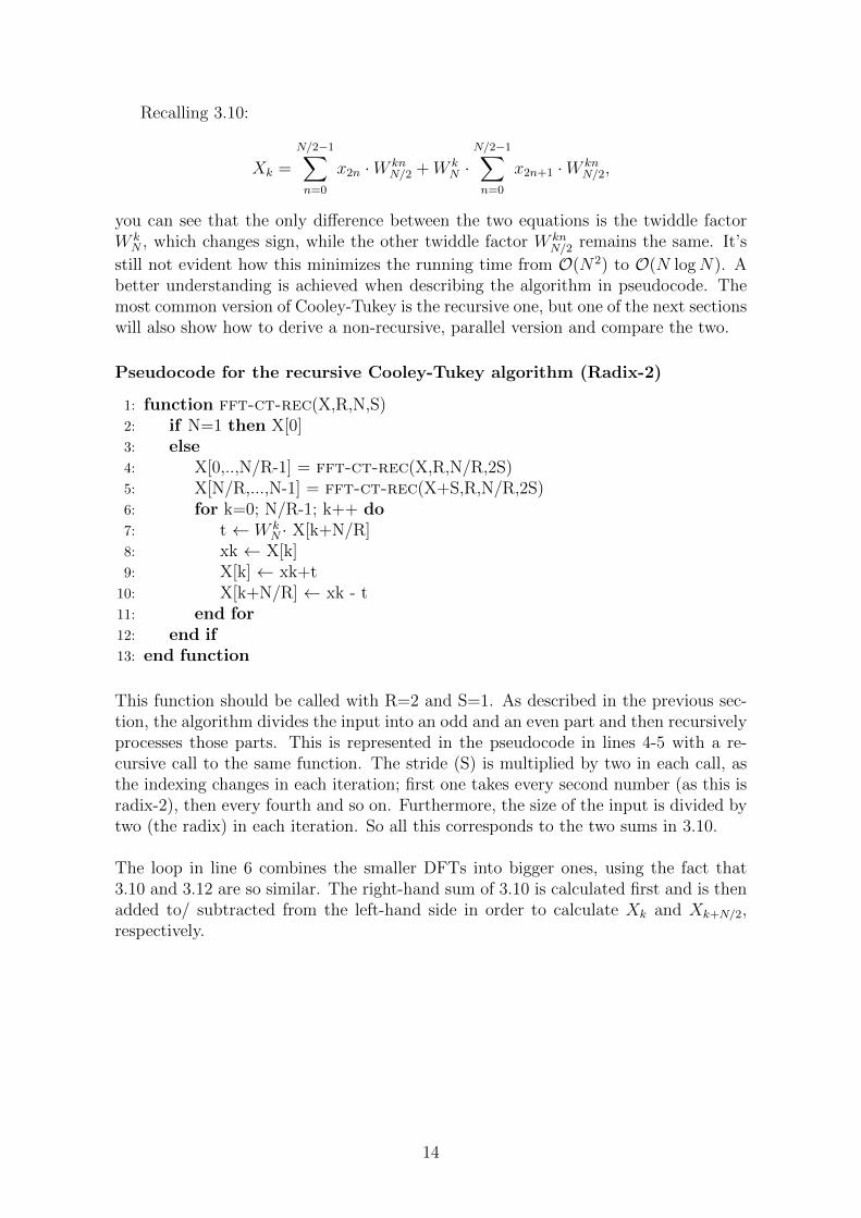
still not evident how this minimizes the running time from O(N2) to O(N logN). Abetter understanding is achieved when describing the algorithm in pseudocode. Themost common version of Cooley-Tukey is the recursive one, but one of the next sectionswill also show how to derive a non-recursive, parallel version and compare the two.
Pseudocode for the recursive Cooley-Tukey algorithm (Radix-2)
1: function fft-ct-rec(X,R,N,S)2: if N=1 then X[0]3: else4: X[0,..,N/R-1] = fft-ct-rec(X,R,N/R,2S)5: X[N/R,...,N-1] = fft-ct-rec(X+S,R,N/R,2S)6: for k=0; N/R-1; k++ do7: t ← W k
N · X[k+N/R]8: xk ← X[k]9: X[k] ← xk+t10: X[k+N/R] ← xk - t11: end for12: end if13: end function
This function should be called with R=2 and S=1. As described in the previous sec-tion, the algorithm divides the input into an odd and an even part and then recursivelyprocesses those parts. This is represented in the pseudocode in lines 4-5 with a re-cursive call to the same function. The stride (S) is multiplied by two in each call, asthe indexing changes in each iteration; first one takes every second number (as this isradix-2), then every fourth and so on. Furthermore, the size of the input is divided bytwo (the radix) in each iteration. So all this corresponds to the two sums in 3.10.
The loop in line 6 combines the smaller DFTs into bigger ones, using the fact that3.10 and 3.12 are so similar. The right-hand sum of 3.10 is calculated first and is thenadded to/ subtracted from the left-hand side in order to calculate Xk and Xk+N/2,respectively.
14
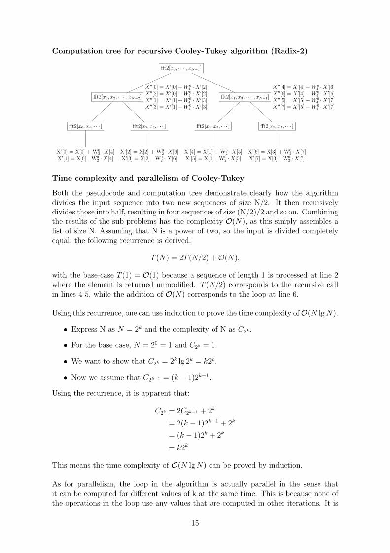
Computation tree for recursive Cooley-Tukey algorithm (Radix-2)
fft2[x0, · · · , xN−1]
fft2[x0, x2, · · · , xN−2]
X ′′[0] = X ′[0] +W 04 ·X ′[2]
X ′′[2] = X ′[0]−W 04 ·X ′[2]
X ′′[1] = X ′[1] +W 04 ·X ′[3]
X ′′[3] = X ′[1]−W 04 ·X ′[3]
fft2[x0, x4, · · · ]
X’[0] = X[0] + W02 ·X[4]
X’[1] = X[0] - W02 ·X[4]
fft2[x2, x6, · · · ]
X’[2] = X[2] + W02 ·X[6]
X’[3] = X[2] - W02 ·X[6]
fft2[x1, x3, · · · , xN−1]
X ′′[4] = X ′[4] +W 04 ·X ′[6]
X ′′[6] = X ′[4]−W 04 ·X ′[6]
X ′′[5] = X ′[5] +W 04 ·X ′[7]
X ′′[7] = X ′[5]−W 04 ·X ′[7]
fft2[x1, x5, · · · ]
X’[4] = X[1] + W02 ·X[5]
X’[5] = X[1] - W02 ·X[5]
fft2[x3, x7, · · · ]
X’[6] = X[3] + W02 ·X[7]
X’[7] = X[3] - W02 ·X[7]
Time complexity and parallelism of Cooley-Tukey
Both the pseudocode and computation tree demonstrate clearly how the algorithmdivides the input sequence into two new sequences of size N/2. It then recursivelydivides those into half, resulting in four sequences of size (N/2)/2 and so on. Combiningthe results of the sub-problems has the complexity O(N), as this simply assembles alist of size N. Assuming that N is a power of two, so the input is divided completelyequal, the following recurrence is derived:
T (N) = 2T (N/2) +O(N),
with the base-case T (1) = O(1) because a sequence of length 1 is processed at line 2where the element is returned unmodified. T (N/2) corresponds to the recursive callin lines 4-5, while the addition of O(N) corresponds to the loop at line 6.
Using this recurrence, one can use induction to prove the time complexity ofO(N lgN).
• Express N as N = 2k and the complexity of N as C2k .
• For the base case, N = 20 = 1 and C20 = 1.
• We want to show that C2k = 2k lg 2k = k2k.
• Now we assume that C2k−1 = (k − 1)2k−1.
Using the recurrence, it is apparent that:
C2k = 2C2k−1 + 2k
= 2(k − 1)2k−1 + 2k
= (k − 1)2k + 2k
= k2k
This means the time complexity of O(N lgN) can be proved by induction.
As for parallelism, the loop in the algorithm is actually parallel in the sense thatit can be computed for different values of k at the same time. This is because none ofthe operations in the loop use any values that are computed in other iterations. It is
15

evident when looking at the computation tree, as each of the leaves can be computedby themselves and combing two nodes is also independent from combining two othernodes at the same level. However, there are certainly dependencies between the differ-ent levels of the tree. The next section will take a look at the parallel Cooley-Tukeyalgorithm that can be derived from the computation tree.
Pseudocode for parallel Cooley-Tukey algorithm (Radix-2)
1: function fft-ct-parallel(X,N,R,bits)2: R = 23: Y = malloc space4: Z = malloc space5: twiddles ← map (x -> twiddle(x)) [1 · · ·n− 1]6: offset ← 07: for i=0; i<bits; i++ do8: for j=0; j<N/R-1; j++ do9: Ns ← 2i
10: t ← twiddles[offset+(j%Ns)]11: idx ← ((j/Ns)*Ns*R) + (j%Ns)12: Y[idx] ← X[idx] + t13: Y[idx + Ns] ← X[idx + N/R] - t14: Z ← X15: X ← Y16: Y ← Z17: offset ← offset + 2i
18: end for19: end for20: end function
The parallel Cooley-Tukey algorithm is quite similar to the recursive one, but insteadof depth-first, it uses a breadth-first search to calculate the nodes of the computationtree. The twiddle factors are precomputed as there is a fixed amount of them. Doublebuffering is used to ensure the parallelism of the inner loop; first, the computed valuesfor the output array are re-written into an entirely new array Y (lines 12-13). Then,the current output array is saved into Z (line 13) and afterwards the new value iswritten into the output array (line 15). Finally, Y is changed to contain the values ofthe output array. This results in a lack of data dependency in the inner loop, whichmay now be executed in parallel.
3.2.2 Stockham
One of the many other FFT algorithms based on Cooley-Tukey is the Stockham auto-sort FFT [18]. Let us take a look at the Stockham algorithm for radix-2 and 4. Sofar this study has only looked at radix-2, but there is an endless amount of differentradix for FFT algorithms. The radix-4 algorithm divides the input into four piecesinstead of two, which means one needs to compute four indexes and four values in eachiteration.
16

Pseudocode for the Stockham radix-2 algorithm
1: function fft-stockham(X,N,R)2: R = 23: Z = malloc space4: Y = malloc space5: for Ns = 1; Ns < N; Ns *= R do6: for j=0; j<N/R ; j++ do
7: t ← W j%NsNs·R · X[j+N/R]
8: Y[(j/Ns)*Ns*R + (j%Ns)] ← X[j] + t9: Y[(j/Ns)*Ns*R + (j%Ns) + Ns] ← X[j] - t10: Z ← X11: X ← Y12: Y ← Z13: end for14: end for15: end function
Pseudocode for the Stockham radix-4 algorithm
1: function fft-stockham(X,N,R)2: R = 43: Z = malloc space4: Y = malloc space5: for Ns = 1; Ns < N; Ns *= R do6: for j=0; j<N/R ; j++ do
7: t1 ← W j%NsNs·R · X[j+N/R]
8: t3 ← W j%NsNs·R · X[j+3N/R]
9: Y[(j/Ns)*Ns*R + (j%Ns)] ← X[j] + X[j+2*N/R] + t1 + t310: Y[(j/Ns)*Ns*R + (j%Ns) + Ns] ← X[j] - X[j+2*n/r] + t1 − t311: Y[(j/Ns)*Ns*R + (j%Ns)+2*Ns ← X[j] + X[j+2*N/R] - t1 − t312: Y[(j/Ns)*Ns*R + (j%Ns)+3*Ns ← X[j] - X[j+2*n/r] - t1 + t313: Z ← X14: X ← Y15: Y ← Z16: end for17: end for18: end function
Similar to the parallel Cooley-Tukey algorithm, the algorithm uses a breadth-firstapproach to calculate all the values, which promotes parallel execution as discussedpreviously. However, it uses a different sorting network than Cooley-Tukey. But sincethe parallel Cooley-Tukey algorithm has already been derived, this one should be easyto understand. Note that the twiddle factors could be calculated beforehand, but asthey commonly are not, that optimization hasn’t been included in the pseudocode.Most of the inner loop is parallel due to the double-buffering; each of the four calcula-tions reads from one array and writes to another, similar to the parallel Cooley-Tukeyalgorithm. Furthermore, each iteration is independent from the others.
17

3.2.3 Factorization and Hierarchical FFT
Factorization of an input sequence has the potential to optimize the calculation of anFFT further. If the length N of an sequence can be factorized so that N = N1 · N2,one can also re-write n = n1N2 + n2 and k = k1 + k2N1 and then substitute into theDFT formula 3.5 (Xk =
∑N−1n=0 xnW
knN ):
Xk1+k2N1 =
N1N2−1∑n1n2=0
xn1N2+n2W(k1+k2N1)(n1N2+n2)N1N2
=
N2−1∑n2=0
N1−1∑n1=0
xn1N2+n2 · e−2πiN1N2
(k1+k2N1)(n1N2+n2)
=
N2−1∑n2=0
N1−1∑n1=0
xn1N2+n2 · e−2πiN1N2
(k1n1N2+k1n2+k2N1n1N2+k2N1n2)
=
N2−1∑n2=0
N1−1∑n1=0
xn1N2+n2 · e−2πiN1
k1n1 · e−2πiN
k1n2 · e−2πik2n1 · e−2πiN2
k2N1n2
=
N2−1∑n2=0
[(N1−1∑n1=0
xn1N2+n2Wk1n1N1
)W k1n2N
]W k2n2N2
, (3.13)
[6]. Note that the factor e−2πik2n1 vanishes, as e−2πix = 1 for all integers x.
Imagine the input sequence as a 2-D matrix of size N1 x N2. The FFT can be computedaccording to 3.13 by following these steps, known as hierarchical FFT computation:
1. Perform N2 FFTs column-wise. This corresponds to the inner sum in 3.13.The column number N2 is fixed from the outside, while the row number N1 isinvariant.i
2. Multiply with the twiddle factors W k1n2N .
3. Perform N1 FFTs row-wise; one FFT per N1, which are the number of rows.This corresponds to the outer sum in 3.13. These are performed on the resultfrom step 2.
4. Transpose the result from step 3.ii
The best way to divide N depends on a variety of factors, such as the length of theinput sequence and the block-size of the system, but this issue will be addressed whendiscussing how to implement factorization.
iAn easy way to compute this is in parallel is to transpose the array, then perform the FFTsrow-wise (on the previous columns), and then transpose back the result.
iiThe original matrix has the dimensions N1 x N2, but the indexing of the result Xk1+k2N1is that
of the transposed matrix, which has the dimensions N2 x N1.
18

Chapter 4
Modularity
The main objective of this thesis is to study a performance-oriented generic FFTimplementation in Futhark, as well as the software engineering concerns that wouldallow several implementations of FFTs to be combined into one library in a way thatis transparent for the user.
The suggested implementation contains a generic representation of the radix thatminimizes code clones from the current Futhark FFT library, and analyzes the currentdata-set to discriminate the optimal implementation for the specific data-set. It alsoallows the user to choose between using a global or shared memory FFT implementa-tion, and uses algorithmic optimization such as pre-computation of the twiddle factors.
This chapter describes the implementation and organization of the FFT library. Theextended source code can be found in the appendix.
4.1 Modules
In order to maintain a high level of flexibility and reduce code complexity, I split theimplementation of the library into three Futhark modules with the following mainfunctionalities:
1. The FFT iteration. A module that implements the calculation of an FFT fora sequence that has the length of the radix (2, 4, 8 etc.).
2. The main functions of the FFT algorithm. A parametric module thatreceives an iteration module and implements the skeleton of the FFT algorithm;a loop with lgN iterations which updates and shuffles the elements in eachiteration.
3. The creation and execution of a plan. A module that creates a plan bytaking the input size N and pre-computes all the information that depends onN only. Then, that plan can be executed as many times as needed. The userreceives no information on how the plan was created, i.e. what radix is used etc.
I will describe the implementation of these on a general level in the following sections,and zoom in on more specific parts of the implementation in relation to global vs.shared memory FFTs afterwards.
19

4.1.1 Rationale of the Structure
This section takes a look at the current radix-2 specialized Futhark implementationof an FFT library, and explains what changes were necessary in order to implement ageneric representation of the radix.
1 let fft_iteration [n] (forward: f32) (ns: i32) (data: [n]complex) (j: i32) :
2 (i32 , complex , i32 , complex) =
3 let angle = (-2f32 * forward * f32.pi * r32 (j % ns)) / r32 (ns * radix)
4 let (v0, v1) = (data[j], data[j+n/radix] complex .*
5 (complex.mk (f32.cos angle) (f32.sin angle )))
6 let (v0, v1) = (v0 complex .+ v1 , v0 complex.- v1)
7 let idxD = ((j/ns)*ns*radix) + (j % ns)
8 in (idxD , v0, idxD+ns, v1)
Listing 4.1: FFT iteration function for radix-2
This function implements the functionality of a single FFT iteration, more preciselyone iteration of the inner for-loop in the Stockham radix-2 algorithm (section 3.2.2).
The twiddle factor is computed in lines 4-5, where the angle or W j%NsNs·R is multiplied
with X[j+N/R]. The return values are calculated by adding the twiddle factor to X[j]and subtracting it from X[j+N/R] in line 6. The indices calculated in lines 7-8 are theexact same ones as in the Stockham algorithm.
The fft_iteration function is called by the fft’ function, which corresponds tofft-stockham as presented in (section 3.2.2).
1 let fft ’ [n] (forward: f32) (input: [n]complex) (bits: i32) : [n]complex =
2 let input = intrinsics.cosmin_flatten (copy (intrinsics.unflatten
3 (n/radix , radix , input )))
4 let output = intrinsics.cosmin_flatten (copy (intrinsics.unflatten
5 (n/radix , radix , input )))
6 let ix = iota(n/radix)
7 let NS = map (radix **) (iota bits)
8 let (res ,_) =
9 loop (input ’: *[n]complex , output ’: *[n]complex) = (input , output)
10 for ns in NS do
11 let (i0s , i1s , v0s , v1s) =
12 unsafe (unzip
13 (map (fft_iteration forward ns input ’) ix))
14 in (scatter output ’ (i0s ++ i1s) (v0s ++ v1s), input ’)
15 in res
Listing 4.2: FFT main function for radix-2
Denoting radix by r, the array NS created at line 7, holds values [r0, r1,. . ., n/r]
(because bits is logr n and iota q, creates the array [0,. . .,q-1] for some q). Theloop between lines 9 and 14, executes sequentially bits iterations, in which the valuesof ns are (consecutively) taken from the elements of array NS. The variables whosevalues are variant to the loop, i.e., input’ and output’, are initialized to input andoutput and are bound in order to the result of the loop body (line 14) for the nextiteration.
Note that the implementation of the loop uses double buffering, since the scatter-updated value of output’ is bound to loop-variant array input’ for the next iteration.Similarly, the map at line 13 implements the innermost loop in the FFT pseudocode,and operates on array ix, which is constant and is initialized at line 6 with [0,. . .,n/r-1]. The result of the map is unzipped, resulting in 2 arrays of indexes and 2 arrays of
20
values (r = radix). Finally, the two index and the two values arrays are concatenatedinto two arrays, based on which, the array combinator scatter distributes the results(line 14).
If one was to implement these functions for radix-4, fft_iteration would returna tuple of four indices and four values. It follows that the return type would be differ-ent from radix-2. This goes on to have an effect on line 11 in fft’, which would alsohave four arrays of indexes and four arrays of values, so that scatter would have tooperate at line 14 on a concatenation of four index and four value arrays, respectively.As all of these differences are type-based, an evident solution is to create abstractedtypes that depend on the radix.
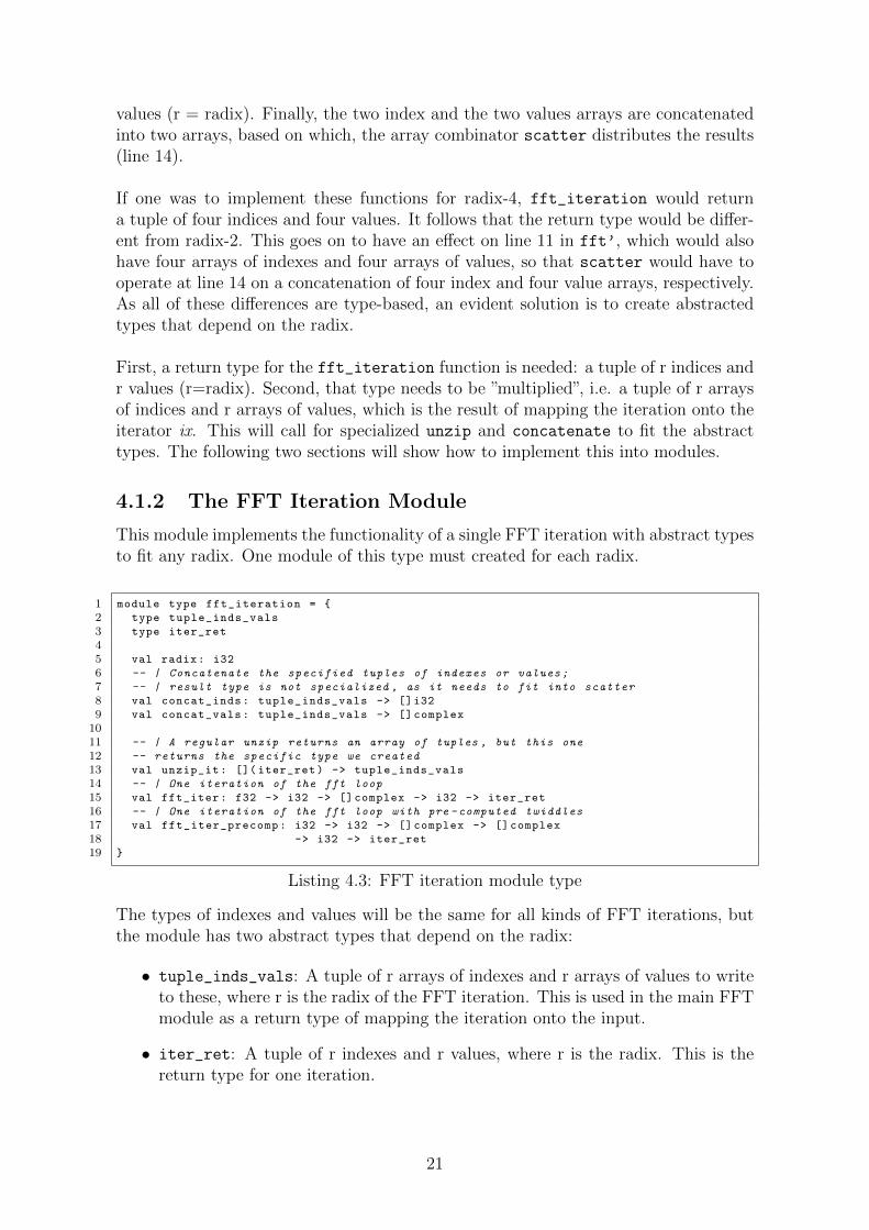
First, a return type for the fft_iteration function is needed: a tuple of r indices andr values (r=radix). Second, that type needs to be ”multiplied”, i.e. a tuple of r arraysof indices and r arrays of values, which is the result of mapping the iteration onto theiterator ix. This will call for specialized unzip and concatenate to fit the abstracttypes. The following two sections will show how to implement this into modules.
4.1.2 The FFT Iteration Module
This module implements the functionality of a single FFT iteration with abstract typesto fit any radix. One module of this type must created for each radix.
1 module type fft_iteration = {
2 type tuple_inds_vals
3 type iter_ret
45 val radix: i32
6 -- | Concatenate the specified tuples of indexes or values;
7 -- | result type is not specialized , as it needs to fit into scatter
8 val concat_inds: tuple_inds_vals -> []i32
9 val concat_vals: tuple_inds_vals -> [] complex
1011 -- | A regular unzip returns an array of tuples , but this one
12 -- returns the specific type we created
13 val unzip_it: []( iter_ret) -> tuple_inds_vals
14 -- | One iteration of the fft loop
15 val fft_iter: f32 -> i32 -> [] complex -> i32 -> iter_ret
16 -- | One iteration of the fft loop with pre -computed twiddles
17 val fft_iter_precomp: i32 -> i32 -> [] complex -> [] complex
18 -> i32 -> iter_ret
19 }
Listing 4.3: FFT iteration module type
The types of indexes and values will be the same for all kinds of FFT iterations, butthe module has two abstract types that depend on the radix:
• tuple_inds_vals: A tuple of r arrays of indexes and r arrays of values to writeto these, where r is the radix of the FFT iteration. This is used in the main FFTmodule as a return type of mapping the iteration onto the input.
• iter_ret: A tuple of r indexes and r values, where r is the radix. This is thereturn type for one iteration.
21

For the main function of the module, there are two variations: one with pre-computedtwiddle factors, and one without. There are some code clones between the two vari-ations, which is something that could be improved in the future. I will discuss pre-computation of the twiddle factors in the section regarding global memory FFTs andonly explain the regular version here.
1 module fft_iteration2: (fft_iteration) = {
2 type ind = i32
3 type vl = complex
4 type inds = []ind
5 type vals = []vl
6 type tuple_inds_vals = (inds , inds , vals , vals)
7 type iter_ret = (ind , ind , vl, vl)
89 let radix = 2i32
10 let concat_inds ((a,b,_,_): tuple_inds_vals) = concat a b
11 let concat_vals ((_,_,c,d): tuple_inds_vals) = concat c d
1213 let unzip_it (x: []( iter_ret )) = unzip x
14 let fft_iter [n] (forward: f32) (ns: i32) (data: [n]complex) (j: i32) : (iter_ret) =
15 let angle = (-2f32 * forward * f32.pi * r32 (j % ns)) / r32 (ns * radix)
16 let (v0, v1) = (data[j], data[j+n/radix] complex .*
17 (complex.mk (f32.cos angle) (f32.sin angle )))
18 let (v0, v1) = (v0 complex .+ v1 , v0 complex.- v1)
19 let idxD = ((j/ns)*ns*radix) + (j % ns)
20 in (idxD , idxD+ns, v0, v1)
Listing 4.4: FFT iteration module for radix-2
This implementation only differs from the radix-2 specialized one (see subsection 4.1.1)in using the abstract return type iter_ret (line 7) instead of a regular tuple of indexesand values.
1 module fft_iteration4: (fft_iteration) = {
2 type ind = i32
3 type vl = complex
4 type inds = []ind
5 type vals = []vl
6 type tuple_inds_vals = (inds , inds , inds , inds ,
7 vals , vals , vals , vals)
8 type iter_ret = (ind , ind , ind , ind , vl, vl, vl, vl)
910 let radix = 4i32
11 let concat_inds ((a,b,c,d,_,_,_,_): tuple_inds_vals) = a ++ b ++ c ++ d
12 let concat_vals ((_,_,_,_,a,b,c,d): tuple_inds_vals) = a ++ b ++ c ++ d
1314 let unzip_it (x: []( iter_ret )) = unzip x
15 let twiddle (a: complex) : complex =
16 complex.mk (complex.im a) (- (complex.re a))
1718 let fft_iter [n] (forward: f32) (ns: i32) (data: [n]complex) (j: i32)
19 : (iter_ret) =
20 let angle = (-2f32 * forward * f32.pi * r32 (j%ns)) / r32 (ns * radix)
21 let tw = complex.mk (f32.cos angle) (f32.sin angle)
22 let a0 = data[j]
23 let a1 = tw complex .* (data[j+n/radix])
24 let a2 = data[j+2*n/radix]
25 let a3 = tw complex .* (data[j+3*n/radix])
2627 let tw = tw complex .* tw
28 let a2 = tw complex .* a2
29 let a3 = tw complex .* a3
3031 let b0 = a0 complex .+ a2
32 let b1 = a0 complex.- a2
33 let b2 = a1 complex .+ a3
34 let b3 = twiddle (a1 complex.- a3)
22

3536 let v0 = b0 complex .+ b2
37 let v2 = b0 complex.- b2
38 let v1 = b1 complex .+ b3
39 let v3 = b1 complex.- b3
4041 let idxD = ((j/ns)*ns*radix) + (j % ns)
42 in (idxD , idxD+ns, idxD +2*ns, idxD +3*ns, v0, v1, v2, v3)
Listing 4.5: FFT iteration module for radix-4
The radix-4 module implementation follows the algorithm described in section 3.2.2.Although it returns a different tuple than the radix-2 module, it fits the iter_ret typespecified in this module (line 8). All other functions and types are also specialized forradix-4. Lines 21-38 are slightly more verbose than the pseudocode in order to makethe computation of radix-4 FFT values more clear.
Trivial functionality of the iteration module is an implementation of the radix (line 2),functions to concatenate the indexes and values with each other (lines 11-12), as wellas an unzip function for the specified types (line 14).
4.1.3 The Main FFT Module
This module implements the main functionality of the FFT for complex and real input.
1 module type fft_module = {
2 val radix: i32
3 -- | Find out whether input size is a power of the radix
4 val powOfR: i32 -> bool
5 -- | FFT of complex numbers
6 val fft [n]: [n](f32 , f32) -> bool -> [n](f32 , f32)
7 -- | FFT of 2-D array of complex numbers for factorization
8 val fact: [][](f32 ,f32) -> i32 -> [](f32 , f32)
9 -- | FFT of real numbers
10 val fft_real [n]: [n]f32 -> bool -> [n]f32
11 }
Listing 4.6: FFT main module type
Modules with this type should be parametric, meaning they take an FFT iterationmodule as input and produce an FFT module. This way, they use the same radix asthe specified iteration module.
1 module fft_module(Iter: fft_iteration ): fft_module = {
2 let radix = Iter.radix
3 ...
4 }
Listing 4.7: Parametric FFT module
The function of interest in this module is fft, which computes the FFTs for complexinput. For real numbers, the input is converted into complex numbers, transformedwith fft and then converted back to real format, as the following code exemplifies:
1 let fft_real [n] (data: [n]f32) (precomp: bool): ([n]f32) =
2 map (\r -> complex.re r)
3 (fft (map (\r -> complex.mk_re r) data) (precomp ))
Listing 4.8: FFT for real input
23

The boolean parameter precomp specifies whether a pre-computation of the twiddlefactors should be performed. If the input is real, that information is sent on to fft,otherwise it is specified there.
1 let generic_fft [n] (forward: bool) (data: [n](f32 ,f32)) (precomp: bool):
2 [n](f32 ,f32) =
3 let n_bits = logR n
4 let forward ’ = if forward then 1f32 else -1f32
5 in if (precomp == false) then take n (fft ’ forward ’ data n_bits)
6 else take n (fft_precomp ’ forward ’ data n_bits)
78 let fft [n] (data: [n](f32 , f32)) (precomp: bool): [n](f32 , f32) =
9 generic_fft true data precomp
Listing 4.9: FFT wrapper function
The fft function is actually a wrapper function that calls a more generic function,which is a wrapper for forward and inverse FFTs. For inverse FFTs, generic_fft iscalled with the parameter forward set to false. The generic function now calls fft’,which is where the actual implementation of the FFT algorithm is hidden. Dependingon whether pre-computation of the twiddle factors is demanded, fft_precomp’ canbe chosen as well, but this will be discussed in the global memory FFT chapter.
1 let fft ’ [n] (forward: f32) (input: [n]complex) (bits: i32) : [n]complex =
2 let input = intrinsics.cosmin_flatten (copy (intrinsics.unflatten
3 (n/radix , radix , input )))
4 let output = intrinsics.cosmin_flatten (copy (intrinsics.unflatten
5 (n/radix , radix , input )))
6 let ix = iota(n/radix)
7 let NS = map (radix **) (iota bits)
8 let (res ,_) =
9 loop (input ’: *[n]complex , output ’: *[n]complex) = (input , output)
10 for ns in NS do
11 let (inds_vals: Iter.tuple_inds_vals) =
12 unsafe (Iter.unzip_it
13 (map (Iter.fft_iter forward ns input ’) ix))
14 in (scatter output ’ (Iter.concat_inds inds_vals)
15 (Iter.concat_vals inds_vals), input ’)
16 in res
Listing 4.10: FFT main function for generic radix
This implementation is quite similar to the radix-2 specialized one (see section 4.1.1),but it is using a version of fft_iter that returns the abstract type iter_ret - a tupleof r indices and r values, r being the radix. This type is ”hidden” in the above codethough, because the above function uses the iteration function in a map over [1..N/R](lines 6 and 13). This returns an array of length (N/radix) of iteration results insteadof a single result of type iter_ret.
As the indices and values need to be separated, essentially the SOAC unzip (line12) is used to change the array of iteration results into a tuple of r arrays of indicesand r arrays of values. This is the second abstract type from the iteration module,tuple_inds_vals.
24
The use of the abstract type calls for a specialized unzip function that returns thistype, which has been implemented in the iteration module. Futhermore, in order toconcatenate the indices and values with each other respectively in a generic way, twospecialized concatenate functions are implemented, which will concatenate either ther index arrays (line 14) or the r value arrays (line 15) with each other. In the function,the map in line 13 and scatter in line 14 are fused together by the compiler in orderto increase parallelization.
A trivial functionality of the fft module is the function powOfR to determine whetherthe input size is a power of the radix, which can be useful in deciding how to split theinput for shared memory FFTs. The module also contains a function fact to computeFFTs of 2-dimensional input for factorization. This will be discussed in detail in anupcoming section on shared memory FFTs.
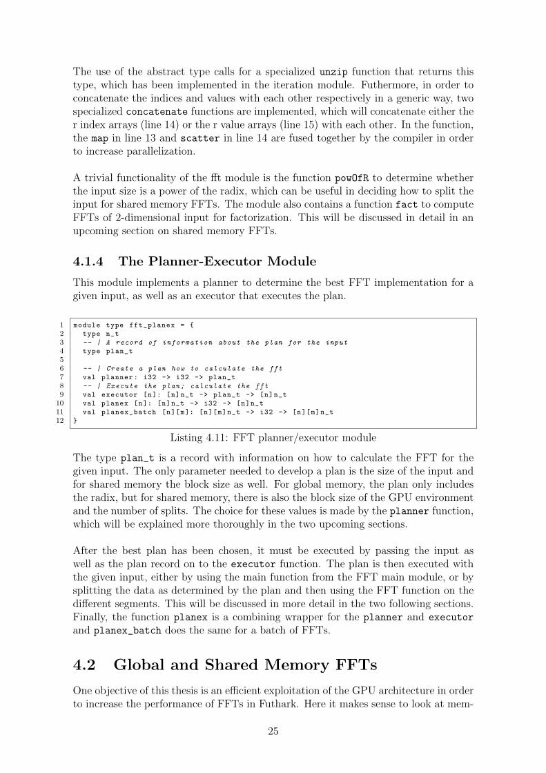
4.1.4 The Planner-Executor Module
This module implements a planner to determine the best FFT implementation for agiven input, as well as an executor that executes the plan.
1 module type fft_planex = {
2 type n_t
3 -- | A record of information about the plan for the input
4 type plan_t
56 -- | Create a plan how to calculate the fft
7 val planner: i32 -> i32 -> plan_t
8 -- | Execute the plan; calculate the fft
9 val executor [n]: [n]n_t -> plan_t -> [n]n_t
10 val planex [n]: [n]n_t -> i32 -> [n]n_t
11 val planex_batch [n][m]: [n][m]n_t -> i32 -> [n][m]n_t
12 }
Listing 4.11: FFT planner/executor module
The type plan_t is a record with information on how to calculate the FFT for thegiven input. The only parameter needed to develop a plan is the size of the input andfor shared memory the block size as well. For global memory, the plan only includesthe radix, but for shared memory, there is also the block size of the GPU environmentand the number of splits. The choice for these values is made by the planner function,which will be explained more thoroughly in the two upcoming sections.
After the best plan has been chosen, it must be executed by passing the input aswell as the plan record on to the executor function. The plan is then executed withthe given input, either by using the main function from the FFT main module, or bysplitting the data as determined by the plan and then using the FFT function on thedifferent segments. This will be discussed in more detail in the two following sections.Finally, the function planex is a combining wrapper for the planner and executor
and planex_batch does the same for a batch of FFTs.
4.2 Global and Shared Memory FFTs
One objective of this thesis is an efficient exploitation of the GPU architecture in orderto increase the performance of FFTs in Futhark. Here it makes sense to look at mem-
25
ory latency. The latency of global memory on the GPU is a few orders of magnitudehigher than register latency, but there is another type of memory known as sharedmemory, which has a latency comparable to that of register latency. It can be viewedas a user-programmable cache. However, there is a limited supply (v64k) of sharedmemory on each GPU multiprocessor.
This means one can choose to either implement the FFT calculation using global orshared memory. The global memory implementation is a naive implementation thatmainly follows the code examples from the previous sections. However, there are afew possible optimizations, such as pre-computation of the twiddle factor that will bediscussed. The other way is called hierarchical FFT and is aimed at implementing thesequential loop of lgN iterations in shared memory with the goal of increasing perfor-mance. An example and explanation of hierarchical FFT implementation follows afterthe global memory section.
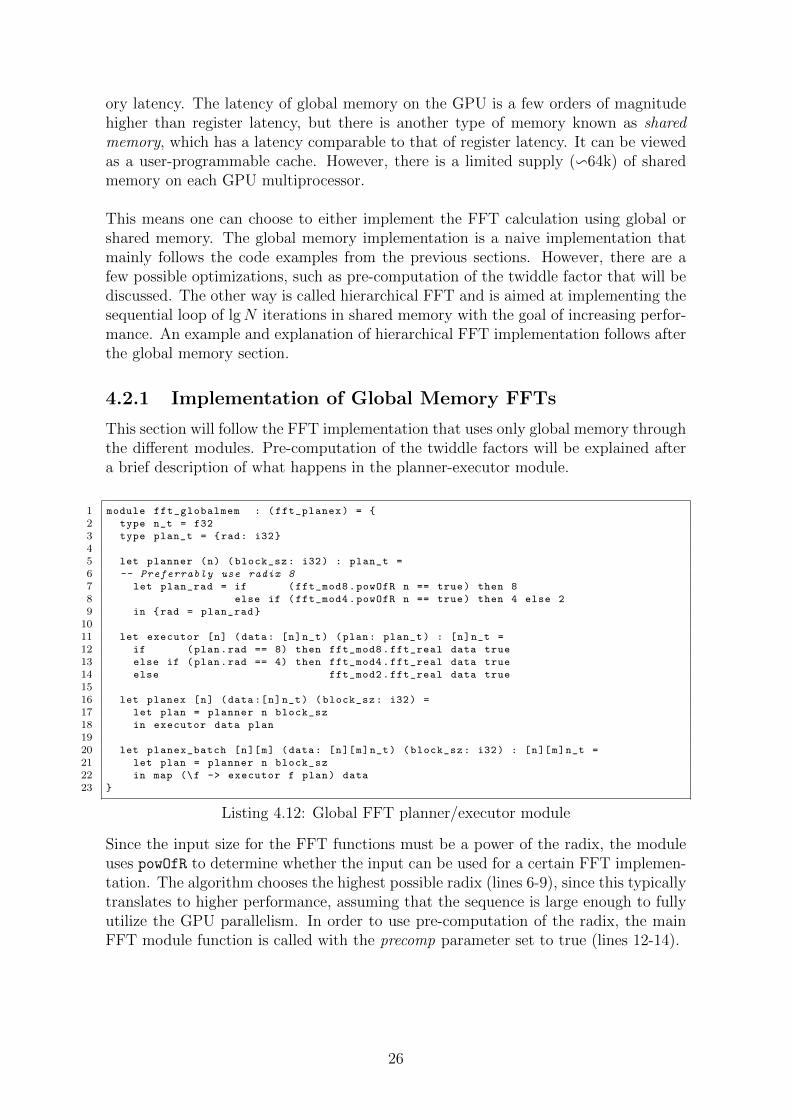
4.2.1 Implementation of Global Memory FFTs
This section will follow the FFT implementation that uses only global memory throughthe different modules. Pre-computation of the twiddle factors will be explained aftera brief description of what happens in the planner-executor module.
1 module fft_globalmem : (fft_planex) = {
2 type n_t = f32
3 type plan_t = {rad: i32}
45 let planner (n) (block_sz: i32) : plan_t =
6 -- Preferrably use radix 8
7 let plan_rad = if (fft_mod8.powOfR n == true) then 8
8 else if (fft_mod4.powOfR n == true) then 4 else 2
9 in {rad = plan_rad}
1011 let executor [n] (data: [n]n_t) (plan: plan_t) : [n]n_t =
12 if (plan.rad == 8) then fft_mod8.fft_real data true
13 else if (plan.rad == 4) then fft_mod4.fft_real data true
14 else fft_mod2.fft_real data true
1516 let planex [n] (data:[n]n_t) (block_sz: i32) =
17 let plan = planner n block_sz
18 in executor data plan
1920 let planex_batch [n][m] (data: [n][m]n_t) (block_sz: i32) : [n][m]n_t =
21 let plan = planner n block_sz
22 in map (\f -> executor f plan) data
23 }
Listing 4.12: Global FFT planner/executor module
Since the input size for the FFT functions must be a power of the radix, the moduleuses powOfR to determine whether the input can be used for a certain FFT implemen-tation. The algorithm chooses the highest possible radix (lines 6-9), since this typicallytranslates to higher performance, assuming that the sequence is large enough to fullyutilize the GPU parallelism. In order to use pre-computation of the radix, the mainFFT module function is called with the precomp parameter set to true (lines 12-14).
26

In a naive FFT implementation, each of the N lgN iterations computes exactly N/rtwiddle factors (r=radix), which leads to some redundant computation. To observethis, recall that in each FFT iteration (see 4.1.2), the angle W k
N for the factor iscomputed using the following formula:
W kN = (2π(j%ns))/(ns · r),
where j indicates which index from [0 · · ·N/r − 1] is being computed and ns is thevalue of the iterator NS = [r0, r1, · · · , rk−1]. For a certain value of ns, the number ofdistinct twiddle factors is in fact ns, due to the modulo operation. For example, forns = 1 there is one twiddle factor and so on upto ns = rk−1. So the total number ofdistinct twiddle factors for all iterations (i.e., elements ns ∈ NS) is:
1 + r + r2 + · · ·+ rk−1 =rk − 1
r − 1=n− 1
r − 1
1 let fft_precomp ’ [n] (forward: f32) (input: [n]complex) (bits: i32) : [] complex =
2 let input = intrinsics.cosmin_flatten
3 (copy (intrinsics.unflatten (n/radix , radix , input )))
4 let output = intrinsics.cosmin_flatten
5 (copy (intrinsics.unflatten (n/radix , radix , input )))
67 -- Precomputation of twiddle factors
8 let wk_ns =
9 map (\ind ->
10 let (n’,ind ’) =
11 loop (s,ind) = (1,ind) while ind >= 0 do
12 (s * radix , ind - s)
13 let k’ = ind ’ + (n’ / radix)
14 let angle = (-2f32 * forward * f32.pi * (r32 k’)) / (r32 n’)
15 in complex.mk (f32.cos angle) (f32.sin angle)
16 ) (iota ((n-1)/( radix -1)))
1718 let ix = iota(n/radix)
19 --let NS = map (radix **) (iota bits)
20 let (res ,_,_) =
21 loop (input ’: *[n]complex , output ’: *[n]complex , offset: i32) =(input , output , 0)
22 for i < bits do
23 let ns = radix ** i
24 let (inds_vals: Iter.tuple_inds_vals) =
25 unsafe (Iter.unzip_it
26 (map
27 (Iter.fft_iter_precomp ns offset wk_ns input ’) ix))
28 in (scatter output ’ (Iter.concat_inds inds_vals)
29 (Iter.concat_vals inds_vals),
30 input ’, offset +(radix**i))
Listing 4.13: Global FFT main function
The pre-computation of the angles happens in the main FFT module inside thefft_precomp’ function. To compute all angles prior to any FFT calculation, a map
over an array of all needed angles is performed (lines 9-16). This works generically forall radix, as the only variables are the size of the input and the radix.
The rest of the function is quite similar to the fft’ function (4.1.3), except thatit has an offset parameter which is used in the iteration module to access the twiddlefactor. This amounts in some code clones that should fixed in future revisions of thecode.
27
1 let fft_iter_precomp [n] (ns: i32) (offset: i32) (wk_ns: [] complex)
2 (data: [n]complex) (j: i32) : (iter_ret) =
3 let k = j % ns
4 let wk_n = unsafe wk_ns[offset+k]
5 let (v0, v1) = (data[j], data[j+n/radix] complex .* wk_n)
6 let (v0, v1) = (v0 complex .+ v1 , v0 complex.- v1)
7 let idxD = ((j/ns)*ns*radix) + (j % ns)
8 in (idxD , idxD+ns, v0, v1)
Listing 4.14: Global FFT iteration radix-2
There is no big difference between the iteration with pre-computed twiddle factors andwithout, except that the twiddle factor does not need to be calculated. Instead, it istaken from wk_ns[offset+k] at line 4, which requires offset as a parameter.
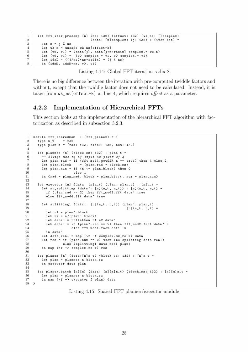
4.2.2 Implementation of Hierarchical FFTs
This section looks at the implementation of the hierarchical FFT algorithm with fac-torization as described in subsection 3.2.3.
1 module fft_sharedmem : (fft_planex) = {
2 type n_t = f32
3 type plan_t = {rad: i32 , block: i32 , num: i32}
45 let planner (n) (block_sz: i32) : plan_t =
6 -- Always use r4 if input is power of 4
7 let plan_rad = if (fft_mod4.powOfR n == true) then 4 else 2
8 let plan_block = (plan_rad * block_sz)
9 let plan_num = if (n <= plan_block) then 0
10 else 1
11 in {rad = plan_rad , block = plan_block , num = plan_num}
1213 let executor [n] (data: [n]n_t) (plan: plan_t) : [n]n_t =
14 let no_splitting (data ’: [n](n_t , n_t)) : [n](n_t , n_t) =
15 if (plan.rad == 2) then fft_mod2.fft data ’ true
16 else fft_mod4.fft data ’ true
1718 let splitting1 (data ’: [n](n_t , n_t)) (plan ’: plan_t) :
19 [n](n_t , n_t) =
20 let n1 = plan ’.block
21 let n2 = n/(plan ’.block)
22 let data ’ = unflatten n1 n2 data ’
23 let data ’ = if (plan ’.rad == 2) then fft_mod2.fact data ’ n
24 else fft_mod4.fact data ’ n
25 in data ’
26 let data_real = map (\r -> complex.mk_re r) data
27 let res = if (plan.num == 0) then (no_splitting data_real)
28 else (splitting1 data_real plan)
29 in map (\r -> complex.re r) res
3031 let planex [n] (data:[n]n_t) (block_sz: i32) : [n]n_t =
32 let plan = planner n block_sz
33 in executor data plan
3435 let planex_batch [n][m] (data: [n][m]n_t) (block_sz: i32) : [n][m]n_t =
36 let plan = planner n block_sz
37 in map (\f -> executor f plan) data
38 }
Listing 4.15: Shared FFT planner/executor module
28
In order to use shared memory, the size of the input Nx on each block should be atmost the product of the radix and the block size: Nx ≤ r ·bs. This is because the inputis divided into r FFTs of size N/r, so they can be run in parallel on different blocks.This suggests that factorization as described in subsection 3.2.3 should be used. Theplanner calculates the maximum block size size and saves it as a part of the plannerobject (line 8). Only radix-2 and radix-4 can be used, and this will be explained inchapter 5, as it has to do with the block size for the machines that the tests wereperfomed on.
Furthermore, the plan includes the information of how often the input should be split.If the input is smaller than the block size, it doesn’t need to split, but otherwise itdoes (lines 9-10). As splitting is only implemented one (i.e. one split into two factors),this is a binary choice. Finally, the plan is executed in the executor.
The executor transforms the input into complex data and checks whether the in-put should be split or not, if not it uses the regular global memory FFT with pre-computation of the twiddle factors (line 15). Otherwise, it splits the data greedilyinto a 2-D matrix of size N1 x N2, where N1 is the highest possible number, i.e. theblock size. N2 is the remaining values of the input (line 21). It then uses the factoriza-tion function discussed below, and in the end transforms the result back to real output.
1 let fact [n1][n2] (data: [n1][n2](f32 ,f32)) (n: i32) : [](f32 , f32) =
2 let data = transpose data
3 let data = map (\d -> fft d false) data
4 -- multiplication with twiddle factors
5 let data = map (\(j2,row) ->
6 map (\(i1,v) ->
7 let angle = (-2f32 * f32.pi * (r32 i1) * (r32 j2)) / (r32 n)
8 let twiddle = complex.mk (f32.cos angle) (f32.sin angle)
9 in v complex .* twiddle
10 ) (zip (iota n1) row)
11 ) (zip (iota n2) data)
12 let data = transpose data
13 let data = map (\d -> fft d false) data
14 in flatten (transpose data)
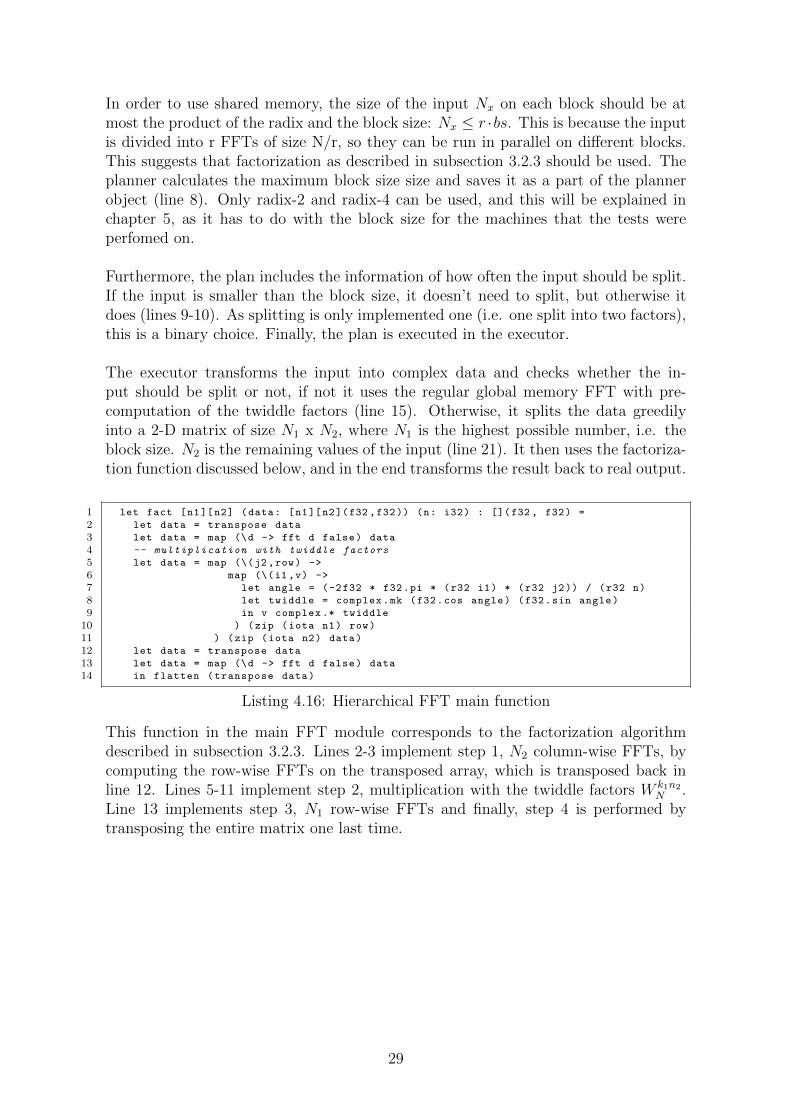
Listing 4.16: Hierarchical FFT main function
This function in the main FFT module corresponds to the factorization algorithmdescribed in subsection 3.2.3. Lines 2-3 implement step 1, N2 column-wise FFTs, bycomputing the row-wise FFTs on the transposed array, which is transposed back inline 12. Lines 5-11 implement step 2, multiplication with the twiddle factors W k1n2
N .Line 13 implements step 3, N1 row-wise FFTs and finally, step 4 is performed bytransposing the entire matrix one last time.
29
Chapter 5
Evaluation
This chapter presents the performance results of the implementation discussed in chap-ter 4. Tests were performed on the DIKU GPU1 machine with an NVIDIA GK110BGPU, as well as an AMD machine with a FirePro AMD GPU. The exact test resultscan be found in the appendix. For each test, a baseline result for performance on theCPU is provided to compare with. As the current implementation does not supportpadding, the applicable data-sets for each radix varied.
5.1 AMD
5.1.1 Method
Benchmarking for global memory was done using the Futhark benchmarking toolfuthark-bench on constant work test files. All test files were compiled using--compiler=futhark-opencl, except when generating data to show the CPU perfor-mance, in which case the futhark-c compiler was used. The size N of the input fileswas 2k where k = [6, 10, 15, 16, 18, 20, 22, 24]. The constant work test files create atesting infrastructure that generates an equal amount of work for each size by creatinga map of size W on top, so that the workload is that the highest k (in our case, it’s24). Recalling that the time complexity / work load of FFT is ON lgN , it should be24 · 224 for an input of size 224. Then for k < 24, W can be found in the following way:
W · k2k = 24 · 224
W = (24 · 224)/(k2k)
W = (24 · 224)/(N lgN)
Hierarchical FFTs were not tested on the AMD GPU, as the results are clear fromthe NVIDIA test in the next section and we didn’t expect an improvement on AMD.Instead, a different kind of shared memory test was executed by compiling the inputwith the flag FUTHARK_INCREMENTAL_FLATTENING=1. This enables shared memory ac-cess and thus only works for low inputs, i.e. where the data-set is smaller than theblock size.
It was not possible to provide a cuFFT baseline, as cuFFT only works on NVIDIAmachines.
30

5.1.2 Expectations
• Higher radix to mostly perform better than lower radix.
• Shared memory to mostly perform better than global memory.
• Pre-computation of twiddle factors to perform better than none.
5.1.3 Results and Discussion
Again, increasing the radix improves the performance in most cases. As on the NVIDIAmachine, radix-4 performs around twice as well as radix-2, while the difference betweenradix-4 and radix-8 is much smaller. Contrary to the NVIDIA GPU test, twiddle fac-tor pre-computation does give a speed-up on the AMD GPU. It is especially significantfor radix-2, and generally most impressive in shared memory.
The shared memory implementation is quite effective, giving just close to a 3x speed-up compared to global memory in the best cases. Unfortunately it is applicable ononly a few datasets. However, radix-8 performs almost the same as radix-4 in sharedmemory. This is because the shared memory version uses r · 2 · 2 (r=radius) words perthread. When r=8, this amount is too high and affects occupancy; there will not beenough memory space for the right amount of blocks on the device. One way to fixthis might be to pre-compute all twiddle factors and not just the angles.
31

5.2 NVIDIA
5.2.1 Method
Testing on the NVIDIA GPU was done in the same way as on the AMD GPU, with afew differences:
For hierarchical FFTs with factorization, benchmarking was done without constantwork, in order to show how the current implementation is only working optimally fora limited input size upto ca. 222. To compare our implementation to the CUDA FFTlibrary cuFFT, a small program was written in CUDA that creates a batch of FFTslike the one used in the Futhark tests.
5.2.2 Expectations
• Higher radix to mostly perform better than lower radix.
• Hierarchical FFT implementation to be optimal up to input size of 222.
• Pre-computation of twiddle factors to perform better than none.
5.2.3 Results and Discussion
The performance of the hierarchical FFT implementation decreases after passing in-put size 222. This was to be expected, as the implementation can only split the inputinto two factors. Recalling that the size of one factor Nx should be Nx ≤ r · bs (seesubsection 4.2.2), where bs = 1024 on NVIDIA, the result will be Nx ≤ 211 for radix-2and Nx ≤ 212 for radix-4. The highest input to be split upto once in this way is thenN = 211 · 211 = 222 for radix-2 and N = 212 · 212 = 224 for radix-4. The input is quiteflat until it reachesNx, since it uses the global memory implementation until that point.
32
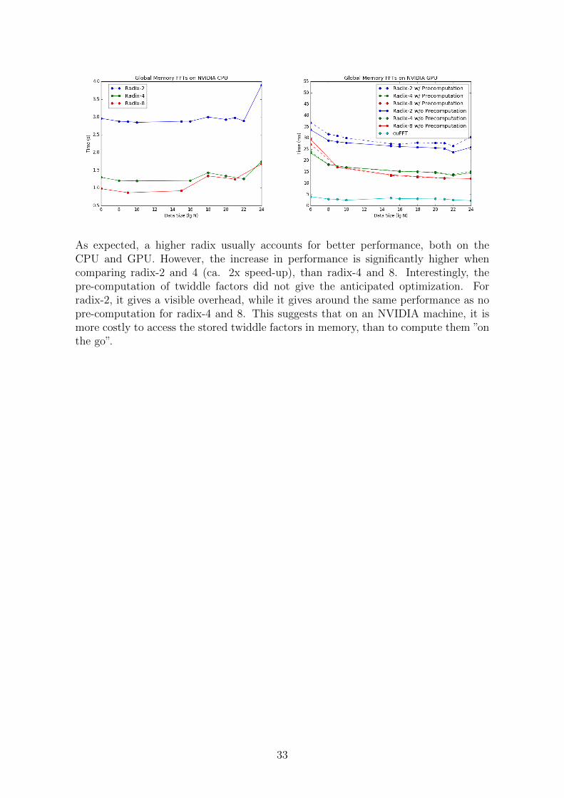
As expected, a higher radix usually accounts for better performance, both on theCPU and GPU. However, the increase in performance is significantly higher whencomparing radix-2 and 4 (ca. 2x speed-up), than radix-4 and 8. Interestingly, thepre-computation of twiddle factors did not give the anticipated optimization. Forradix-2, it gives a visible overhead, while it gives around the same performance as nopre-computation for radix-4 and 8. This suggests that on an NVIDIA machine, it ismore costly to access the stored twiddle factors in memory, than to compute them ”onthe go”.
33
Chapter 6
Conclusion
The thesis presents the implementation of a modular, user-transparent FFT libraryin Futhark, using a generic representation of the radix to minimize code clones. Thelibrary analyzes the input data-set and discriminates the optimal implementation tocalculate its FFT.
The results show that the radix has a significant effect on the performance, with atrend of higher radix giving higher performance. The improvement was more no-ticeable between radix-2 and 4, than between radix-4 and 8. The effect of twiddlefactor pre-computation depends on the specific hardware. For NVIDIA, it lessenedthe performance, indicating that it is more costly to access the stored twiddle factorsin memory, than to compute them ”on the go”. However, pre-computing them didgive a speed-up of up to 2x on AMD GPU. Factorization also seems like a promisingapproach, but as its implementation was restricted, it wasn’t possible to fully test theeffects.
There are still ample improvements to be done to the implementation presented inthis thesis. Most prominently, it will be interesting to see the results for implementingfactorization that splits the input data into more than just two components, since theresults for one splitting are promising. Furthermore, there are still some code clonesin the implementation, particularly in the FFT iteration module. A minimization ofthese is desirable. Lastly, one can experiment with padding of the input in order tobe able to use the optimal radix for a given input, since at this point, a radix-X canonly be used on input that is a power of X.
34
Appendix A
Code
A.1 FFT Iteration Module
import "/ futlib/complex"
module complex = complex f32
type complex = complex.complex
module type fft_iteration = {
type tuple_inds_vals
type iter_ret
val radix: i32
-- | Concatenate the specified tuples of indexes or values;
-- | result type is not specialized , as it needs to fit into scatter
val concat_inds: tuple_inds_vals -> []i32
val concat_vals: tuple_inds_vals -> [] complex
-- | A regular unzip returns an array of tuples , but this one
-- returns the specific type we created
val unzip_it: []( iter_ret) -> tuple_inds_vals
-- | One iteration of the fft loop
val fft_iter: f32 -> i32 -> [] complex -> i32 -> iter_ret
-- | One iteration of the fft loop with pre -computed twiddles
val fft_iter_precomp: i32 -> i32 -> [] complex -> [] complex
-> i32 -> iter_ret
}
-- | Given a radix value , construct a module
-- | implementing specialized fft_iteration for that value
module fft_iteration2: (fft_iteration) = {
type ind = i32
type vl = complex
type inds = []ind
type vals = []vl
type tuple_inds_vals = (inds , inds , vals , vals)
type iter_ret = (ind , ind , vl, vl)
let radix = 2i32
let concat_inds ((a,b,_,_): tuple_inds_vals) = concat a b
let concat_vals ((_,_,c,d): tuple_inds_vals) = concat c d
let unzip_it (x: []( iter_ret )) = unzip x
let fft_iter [n] (forward: f32) (ns: i32) (data: [n]complex) (j: i32) : (iter_ret) =
let angle = (-2f32 * forward * f32.pi * r32 (j % ns)) / r32 (ns * radix)
let (v0, v1) = (data[j], data[j+n/radix] complex .*
(complex.mk (f32.cos angle) (f32.sin angle )))
let (v0, v1) = (v0 complex .+ v1 , v0 complex.- v1)
let idxD = ((j/ns)*ns*radix) + (j % ns)
in (idxD , idxD+ns, v0, v1)
let fft_iter_precomp [n] (ns: i32) (offset: i32) (wk_ns: [] complex)
(data: [n]complex) (j: i32) : (iter_ret) =
35
let k = j % ns
let wk_n = unsafe wk_ns[offset+k]
let (v0, v1) = (data[j], data[j+n/radix] complex .* wk_n)
let (v0, v1) = (v0 complex .+ v1 , v0 complex.- v1)
let idxD = ((j/ns)*ns*radix) + (j % ns)
in (idxD , idxD+ns, v0, v1)
}
module fft_iteration4: (fft_iteration) = {
type ind = i32
type vl = complex
type inds = []ind
type vals = []vl
type tuple_inds_vals = (inds , inds , inds , inds ,
vals , vals , vals , vals)
type iter_ret = (ind , ind , ind , ind , vl, vl, vl, vl)
let radix = 4i32
let concat_inds ((a,b,c,d,_,_,_,_): tuple_inds_vals) = a ++ b ++ c ++ d
let concat_vals ((_,_,_,_,a,b,c,d): tuple_inds_vals) = a ++ b ++ c ++ d
let unzip_it (x: []( iter_ret )) = unzip x
let twiddle (a: complex) : complex =
complex.mk (complex.im a) (- (complex.re a))
let fft_iter [n] (forward: f32) (ns: i32) (data: [n]complex) (j: i32)
: (iter_ret) =
let angle = (-2f32 * forward * f32.pi * r32 (j%ns)) / r32 (ns * radix)
let tw = complex.mk (f32.cos angle) (f32.sin angle)
let a0 = data[j]
let a1 = tw complex .* (data[j+n/radix])
let a2 = data[j+2*n/radix]
let a3 = tw complex .* (data[j+3*n/radix])
let tw = tw complex .* tw
let a2 = tw complex .* a2
let a3 = tw complex .* a3
let b0 = a0 complex .+ a2
let b1 = a0 complex.- a2
let b2 = a1 complex .+ a3
let b3 = twiddle (a1 complex.- a3)
let v0 = b0 complex .+ b2
let v2 = b0 complex.- b2
let v1 = b1 complex .+ b3
let v3 = b1 complex.- b3
let idxD = ((j/ns)*ns*radix) + (j % ns)
in (idxD , idxD+ns, idxD +2*ns, idxD +3*ns, v0, v1, v2, v3)
let fft_iter_precomp [n] (ns: i32) (offset: i32) (wk_ns: [] complex)
(data: [n]complex) (j: i32) : (iter_ret) =
let k = j % ns
let wk_n = unsafe wk_ns[offset+k]
let a0 = data[j]
let a1 = wk_n complex .* (data[j+n/radix])
let a2 = data[j+2*n/radix]
let a3 = wk_n complex .* (data[j+3*n/radix])
let tw = wk_n complex .* wk_n
let a2 = tw complex .* a2
let a3 = tw complex .* a3
let b0 = a0 complex .+ a2
let b1 = a0 complex.- a2
let b2 = a1 complex .+ a3
let b3 = twiddle (a1 complex.- a3)
let v0 = b0 complex .+ b2
let v2 = b0 complex.- b2
let v1 = b1 complex .+ b3
let v3 = b1 complex.- b3
36
let idxD = ((j/ns)*ns*radix) + (j % ns)
in (idxD , idxD+ns, idxD +2*ns, idxD +3*ns, v0, v1, v2, v3)
}
module fft_iteration8: (fft_iteration) = {
type ind = i32
type vl = complex
type inds = []ind
type vals = []vl
type tuple_inds_vals = (inds , inds , inds , inds ,
inds , inds , inds , inds ,
vals , vals , vals , vals ,
vals , vals , vals , vals)
type iter_ret = (ind , ind , ind , ind , ind , ind , ind , ind ,
vl, vl, vl, vl , vl, vl, vl, vl)
let radix = 8i32
let concat_inds ((a,b,c,d,e,f,g,h,_,_,_,_,_,_,_,_):
tuple_inds_vals) = a ++ b ++ c ++ d ++ e ++ f ++ g ++ h
let concat_vals ((_,_,_,_,_,_,_,_,a,b,c,d,e,f,g,h):
tuple_inds_vals) = a ++ b ++ c ++ d ++ e ++ f ++ g ++ h
let unzip_it (x: []( iter_ret )) = unzip x
let sqrt2 = complex.mk (0.707106781188 f32) (0.0 f32)
let twiddle (a: complex) : complex =
complex.mk (complex.im a) (- (complex.re a))
let mul_p1q4(a: complex) : complex =
let x = complex.mk (complex.re a + complex.im a)
(complex.im a - complex.re a)
in x complex .* sqrt2
let mul_p3q4(a: complex) : complex =
let x = complex.mk (complex.im a - complex.re a)
(-(complex.re a) - complex.im a)
in x complex .* sqrt2
let fft_iter [n] (forward: f32) (ns: i32) (data: [n]complex) (j: i32)
: (iter_ret) =
let angle = (-2f32 * forward * f32.pi * r32 (j%ns)) / r32 (ns * radix)
let tw = complex.mk (f32.cos angle) (f32.sin angle)
let a0 = data[j]
let a1 = tw complex .* (data[j+n/radix])
let a2 = data[j+2*n/radix]
let a3 = tw complex .* (data[j+3*n/radix])
let a4 = data[j+4*n/radix]
let a5 = tw complex .* (data[j+5*n/radix])
let a6 = data[j+6*n/radix]
let a7 = tw complex .* (data[j+7*n/radix])
let tw = tw complex .* tw --W^2
let a2 = tw complex .* a2
let a3 = tw complex .* a3
let a6 = tw complex .* a6
let a7 = tw complex .* a7
let tw = tw complex .* tw --W^4
let a4 = tw complex .* a4
let a5 = tw complex .* a5
let a6 = tw complex .* a6
let a7 = tw complex .* a7
let b0 = a0 complex .+ a4
let b4 = a0 complex.- a4
let b1 = a1 complex .+ a5
let b5 = mul_p1q4 (a1 complex.- a5)
let b2 = a2 complex .+ a6
let b6 = twiddle (a2 complex.- a6)
let b3 = a3 complex .+ a7
let b7 = mul_p3q4 (a3 complex.- a7)
let a0 = b0 complex .+ b2
37

let a2 = b0 complex.- b2
let a1 = b1 complex .+ b3
let a3 = twiddle(b1 complex.- b3)
let a4 = b4 complex .+ b6
let a6 = b4 complex.- b6
let a5 = b5 complex .+ b7
let a7 = twiddle(b5 complex.- b7)
let v0 = a0 complex .+ a1
let v4 = a0 complex.- a1
let v1 = a4 complex .+ a5
let v5 = a4 complex.- a5
let v2 = a2 complex .+ a3
let v6 = a2 complex.- a3
let v3 = a6 complex .+ a7
let v7 = a6 complex.- a7
let idxD = ((j/ns)*ns*radix) + (j % ns)
in (idxD , idxD+ns, idxD +2*ns, idxD +3*ns,
idxD +4*ns, idxD +5*ns , idxD +6*ns, idxD +7*ns,
v0, v1, v2, v3, v4, v5, v6, v7)
let fft_iter_precomp [n] (ns: i32) (offset: i32) (wk_ns: [] complex)
(data: [n]complex) (j: i32) : (iter_ret) =
let k = j % ns
let wk_n = unsafe wk_ns[offset+k]
let a0 = data[j]
let a1 = wk_n complex .* (data[j+n/radix])
let a2 = data[j+2*n/radix]
let a3 = wk_n complex .* (data[j+3*n/radix])
let a4 = data[j+4*n/radix]
let a5 = wk_n complex .* (data[j+5*n/radix])
let a6 = data[j+6*n/radix]
let a7 = wk_n complex .* (data[j+7*n/radix])
let tw = wk_n complex .* wk_n --W^2
let a2 = tw complex .* a2
let a3 = tw complex .* a3
let a6 = tw complex .* a6
let a7 = tw complex .* a7
let tw = tw complex .* tw --W^4
let a4 = tw complex .* a4
let a5 = tw complex .* a5
let a6 = tw complex .* a6
let a7 = tw complex .* a7
let b0 = a0 complex .+ a4
let b4 = a0 complex.- a4
let b1 = a1 complex .+ a5
let b5 = mul_p1q4 (a1 complex.- a5)
let b2 = a2 complex .+ a6
let b6 = twiddle (a2 complex.- a6)
let b3 = a3 complex .+ a7
let b7 = mul_p3q4 (a3 complex.- a7)
let a0 = b0 complex .+ b2
let a2 = b0 complex.- b2
let a1 = b1 complex .+ b3
let a3 = twiddle(b1 complex.- b3)
let a4 = b4 complex .+ b6
let a6 = b4 complex.- b6
let a5 = b5 complex .+ b7
let a7 = twiddle(b5 complex.- b7)
let v0 = a0 complex .+ a1
let v4 = a0 complex.- a1
let v1 = a4 complex .+ a5
let v5 = a4 complex.- a5
let v2 = a2 complex .+ a3
let v6 = a2 complex.- a3
let v3 = a6 complex .+ a7
let v7 = a6 complex.- a7
38

let idxD = ((j/ns)*ns*radix) + (j % ns)
in (idxD , idxD+ns, idxD +2*ns, idxD +3*ns,
idxD +4*ns, idxD +5*ns , idxD +6*ns, idxD +7*ns,
v0, v1, v2, v3, v4, v5, v6, v7)
}
A.2 FFT Main Module
import "fft_iteration"
module type fft_module = {
val radix: i32
-- | Find out whether input size is a power of the radix
val powOfR: i32 -> bool
-- | FFT of complex numbers
val fft [n]: [n](f32 , f32) -> bool -> [n](f32 , f32)
-- | FFT of 2-D array of complex numbers for factorization
val fact: [][](f32 ,f32) -> i32 -> [](f32 , f32)
-- | FFT of real numbers
val fft_real [n]: [n]f32 -> bool -> [n]f32
}
module fft_module(Iter: fft_iteration ): fft_module = {
let radix = Iter.radix
let powOfR (n: i32) : bool =
let x = 0i32
let (x, _) = loop (x,n) while ((1 < n) && (x == 0)) do
let x = n % radix
let n = n / radix
in (x, n)
let res = if (x == 0) then true else false
in res
let fft ’ [n] (forward: f32) (input: [n]complex) (bits: i32) : [n]complex =
let input = intrinsics.cosmin_flatten (copy (intrinsics.unflatten
(n/radix , radix , input )))
let output = intrinsics.cosmin_flatten (copy (intrinsics.unflatten
(n/radix , radix , input )))
let ix = iota(n/radix)
let NS = map (radix **) (iota bits)
let (res ,_) =
loop (input ’: *[n]complex , output ’: *[n]complex) = (input , output)
for ns in NS do
let (inds_vals: Iter.tuple_inds_vals) =
unsafe (Iter.unzip_it
(map (Iter.fft_iter forward ns input ’) ix))
in (scatter output ’ (Iter.concat_inds inds_vals)
(Iter.concat_vals inds_vals), input ’)
in res
let fft_precomp ’ [n] (forward: f32) (input: [n]complex) (bits: i32) : [] complex =
let input = intrinsics.cosmin_flatten
(copy (intrinsics.unflatten (n/radix , radix , input )))
let output = intrinsics.cosmin_flatten
(copy (intrinsics.unflatten (n/radix , radix , input )))
-- Precomputation of twiddle factors
let wk_ns =
map (\ind ->
let (n’,ind ’) =
loop (s,ind) = (1,ind) while ind >= 0 do
(s * radix , ind - s)
let k’ = ind ’ + (n’ / radix)
let angle = (-2f32 * forward * f32.pi * (r32 k’)) / (r32 n’)
in complex.mk (f32.cos angle) (f32.sin angle)
) (iota ((n-1)/( radix -1)))
let ix = iota(n/radix)
--let NS = map (radix **) (iota bits)
39

let (res ,_,_) =
loop (input ’: *[n]complex , output ’: *[n]complex , offset: i32) =(input , output , 0)
for i < bits do
let ns = radix ** i
let (inds_vals: Iter.tuple_inds_vals) =
unsafe (Iter.unzip_it
(map
(Iter.fft_iter_precomp ns offset wk_ns input ’) ix))
in (scatter output ’ (Iter.concat_inds inds_vals)
(Iter.concat_vals inds_vals),
input ’, offset +(radix**i))
in res
let logR (n: i32) : i32 =
let r = 0
let (r, _) = loop (r,n) while 1 < n do
let n = n / radix
let r = r + 1
in (r,n)
in r
let generic_fft [n] (forward: bool) (data: [n](f32 ,f32)) (precomp: bool):
[n](f32 ,f32) =
let n_bits = logR n
let forward ’ = if forward then 1f32 else -1f32
in if (precomp == false) then take n (fft ’ forward ’ data n_bits)
else take n (fft_precomp ’ forward ’ data n_bits)
let fft [n] (data: [n](f32 , f32)) (precomp: bool): [n](f32 , f32) =
generic_fft true data precomp
let fact [n1][n2] (data: [n1][n2](f32 ,f32)) (n: i32) : [](f32 , f32) =
let data = transpose data
let data = map (\d -> fft d false) data
-- multiplication with twiddle factors
let data = map (\(j2,row) ->
map (\(i1,v) ->
let angle = (-2f32 * f32.pi * (r32 i1) * (r32 j2)) / (r32 n)
let twiddle = complex.mk (f32.cos angle) (f32.sin angle)
in v complex .* twiddle
) (zip (iota n1) row)
) (zip (iota n2) data)
let data = transpose data
let data = map (\d -> fft d false) data
in flatten (transpose data)
let fft_real [n] (data: [n]f32) (precomp: bool): ([n]f32) =
map (\r -> complex.re r)
(fft (map (\r -> complex.mk_re r) data) (precomp ))
}
A.3 Planner-Executor Module
import "fft_module"
import "fft_iteration"
module iteration2 = fft_iteration2
module fft_mod2 = fft_module(iteration2)
module iteration4 = fft_iteration4
module fft_mod4 = fft_module(iteration4)
module iteration8 = fft_iteration8
module fft_mod8 = fft_module(iteration8)
module type fft_planex = {
type n_t
-- | A record of information about the plan for the input
type plan_t
-- | Create a plan how to calculate the fft
val planner: i32 -> i32 -> plan_t
40

-- | Execute the plan; calculate the fft
val executor [n]: [n]n_t -> plan_t -> [n]n_t
val planex [n]: [n]n_t -> i32 -> [n]n_t
val planex_batch [n][m]: [n][m]n_t -> i32 -> [n][m]n_t
}
module fft_globalmem : (fft_planex) = {
type n_t = f32
type plan_t = {rad: i32}
let planner (n) (block_sz: i32) : plan_t =
-- Preferrably use radix 8
let plan_rad = if (fft_mod8.powOfR n == true) then 8
else if (fft_mod4.powOfR n == true) then 4 else 2
in {rad = plan_rad}
let executor [n] (data: [n]n_t) (plan: plan_t) : [n]n_t =
if (plan.rad == 8) then fft_mod8.fft_real data true
else if (plan.rad == 4) then fft_mod4.fft_real data true
else fft_mod2.fft_real data true
let planex [n] (data:[n]n_t) (block_sz: i32) =
let plan = planner n block_sz
in executor data plan
let planex_batch [n][m] (data: [n][m]n_t) (block_sz: i32) : [n][m]n_t =
let plan = planner n block_sz
in map (\f -> executor f plan) data
}
module fft_sharedmem : (fft_planex) = {
type n_t = f32
type plan_t = {rad: i32 , block: i32 , num: i32}
let planner (n) (block_sz: i32) : plan_t =
-- Always use r4 if input is power of 4
let plan_rad = if (fft_mod4.powOfR n == true) then 4 else 2
let plan_block = (plan_rad * block_sz)
let plan_num = if (n <= plan_block) then 0
else 1
in {rad = plan_rad , block = plan_block , num = plan_num}
let executor [n] (data: [n]n_t) (plan: plan_t) : [n]n_t =
let no_splitting (data ’: [n](n_t , n_t)) : [n](n_t , n_t) =
if (plan.rad == 2) then fft_mod2.fft data ’ true
else fft_mod4.fft data ’ true
let splitting1 (data ’: [n](n_t , n_t)) (plan ’: plan_t) :
[n](n_t , n_t) =
let n1 = plan ’.block
let n2 = n/(plan ’.block)
let data ’ = unflatten n1 n2 data ’
let data ’ = if (plan ’.rad == 2) then fft_mod2.fact data ’ n
else fft_mod4.fact data ’ n
in data ’
let data_real = map (\r -> complex.mk_re r) data
let res = if (plan.num == 0) then (no_splitting data_real)
else (splitting1 data_real plan)
in map (\r -> complex.re r) res
let planex [n] (data:[n]n_t) (block_sz: i32) : [n]n_t =
let plan = planner n block_sz
in executor data plan
let planex_batch [n][m] (data: [n][m]n_t) (block_sz: i32) : [n][m]n_t =
let plan = planner n block_sz
in map (\f -> executor f plan) data
}
41

Appendix B
Benchmarks
B.1 AMD
---------------------
-- FirePro AMD GPU --
---------------------
-----------------------------------------------------------------------
-----------------------------------------------------------------------
-- I. RADIX = 2
1. CPU RUNTIMES:
dataset data/input2pow6.in: 6536544.60us (avg. of 5 runs; RSD: 0.18)
dataset data/input2pow8.in: 6848591.50us (avg. of 10 runs; RSD: 0.01)
dataset data/input2pow9.in: 6046836.20us (avg. of 10 runs; RSD: 0.13)
dataset data/input2pow10.in: 7040947.40us (avg. of 5 runs; RSD: 0.02)
dataset data/input2pow15.in: 6947698.20us (avg. of 5 runs; RSD: 0.06)
dataset data/input2pow16.in: 5244199.40us (avg. of 5 runs; RSD: 0.10)
dataset data/input2pow18.in: 7160000.60us (avg. of 5 runs; RSD: 0.14)
dataset data/input2pow20.in: 6479949.00us (avg. of 5 runs; RSD: 0.10)
dataset data/input2pow21.in: 9106610.80us (avg. of 10 runs; RSD: 0.00)
dataset data/input2pow22.in: 8324531.40us (avg. of 5 runs; RSD: 0.14)
dataset data/input2pow24.in: 11294911.20us (avg. of 5 runs; RSD: 0.02)
2. GPU RUNTIMES: ONLY GLOBAL MEMORY, WITHOUT TWIDDLE PRECOMPUTATION
dataset data/input2pow6.in: 46470.07us (avg. of 30 runs; RSD: 0.05)
dataset data/input2pow8.in: 44250.77us (avg. of 30 runs; RSD: 0.07)
dataset data/input2pow9.in: 43748.83us (avg. of 30 runs; RSD: 0.08)
dataset data/input2pow10.in: 43328.47us (avg. of 30 runs; RSD: 0.08)
dataset data/input2pow15.in: 41551.50us (avg. of 30 runs; RSD: 0.08)
dataset data/input2pow16.in: 41082.73us (avg. of 30 runs; RSD: 0.08)
dataset data/input2pow18.in: 39574.67us (avg. of 30 runs; RSD: 0.08)
dataset data/input2pow20.in: 37232.23us (avg. of 30 runs; RSD: 0.06)
dataset data/input2pow21.in: 33934.27us (avg. of 30 runs; RSD: 0.00)
dataset data/input2pow22.in: 31599.93us (avg. of 30 runs; RSD: 0.01)
dataset data/input2pow24.in: 34159.67us (avg. of 30 runs; RSD: 0.01)
42
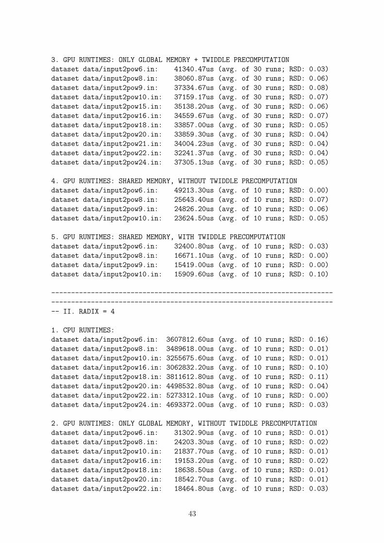
3. GPU RUNTIMES: ONLY GLOBAL MEMORY + TWIDDLE PRECOMPUTATION
dataset data/input2pow6.in: 41340.47us (avg. of 30 runs; RSD: 0.03)
dataset data/input2pow8.in: 38060.87us (avg. of 30 runs; RSD: 0.06)
dataset data/input2pow9.in: 37334.67us (avg. of 30 runs; RSD: 0.08)
dataset data/input2pow10.in: 37159.17us (avg. of 30 runs; RSD: 0.07)
dataset data/input2pow15.in: 35138.20us (avg. of 30 runs; RSD: 0.06)
dataset data/input2pow16.in: 34559.67us (avg. of 30 runs; RSD: 0.07)
dataset data/input2pow18.in: 33857.00us (avg. of 30 runs; RSD: 0.05)
dataset data/input2pow20.in: 33859.30us (avg. of 30 runs; RSD: 0.04)
dataset data/input2pow21.in: 34004.23us (avg. of 30 runs; RSD: 0.04)
dataset data/input2pow22.in: 32241.37us (avg. of 30 runs; RSD: 0.04)
dataset data/input2pow24.in: 37305.13us (avg. of 30 runs; RSD: 0.05)
4. GPU RUNTIMES: SHARED MEMORY, WITHOUT TWIDDLE PRECOMPUTATION
dataset data/input2pow6.in: 49213.30us (avg. of 10 runs; RSD: 0.00)
dataset data/input2pow8.in: 25643.40us (avg. of 10 runs; RSD: 0.07)
dataset data/input2pow9.in: 24826.20us (avg. of 10 runs; RSD: 0.06)
dataset data/input2pow10.in: 23624.50us (avg. of 10 runs; RSD: 0.05)
5. GPU RUNTIMES: SHARED MEMORY, WITH TWIDDLE PRECOMPUTATION
dataset data/input2pow6.in: 32400.80us (avg. of 10 runs; RSD: 0.03)
dataset data/input2pow8.in: 16671.10us (avg. of 10 runs; RSD: 0.00)
dataset data/input2pow9.in: 15419.00us (avg. of 10 runs; RSD: 0.00)
dataset data/input2pow10.in: 15909.60us (avg. of 10 runs; RSD: 0.10)
-----------------------------------------------------------------------
-----------------------------------------------------------------------
-- II. RADIX = 4
1. CPU RUNTIMES:
dataset data/input2pow6.in: 3607812.60us (avg. of 10 runs; RSD: 0.16)
dataset data/input2pow8.in: 3489618.00us (avg. of 10 runs; RSD: 0.01)
dataset data/input2pow10.in: 3255675.60us (avg. of 10 runs; RSD: 0.01)
dataset data/input2pow16.in: 3062832.20us (avg. of 10 runs; RSD: 0.10)
dataset data/input2pow18.in: 3811612.80us (avg. of 10 runs; RSD: 0.11)
dataset data/input2pow20.in: 4498532.80us (avg. of 10 runs; RSD: 0.04)
dataset data/input2pow22.in: 5273312.10us (avg. of 10 runs; RSD: 0.00)
dataset data/input2pow24.in: 4693372.00us (avg. of 10 runs; RSD: 0.03)
2. GPU RUNTIMES: ONLY GLOBAL MEMORY, WITHOUT TWIDDLE PRECOMPUTATION
dataset data/input2pow6.in: 31302.90us (avg. of 10 runs; RSD: 0.01)
dataset data/input2pow8.in: 24203.30us (avg. of 10 runs; RSD: 0.02)
dataset data/input2pow10.in: 21837.70us (avg. of 10 runs; RSD: 0.01)
dataset data/input2pow16.in: 19153.20us (avg. of 10 runs; RSD: 0.02)
dataset data/input2pow18.in: 18638.50us (avg. of 10 runs; RSD: 0.01)
dataset data/input2pow20.in: 18542.70us (avg. of 10 runs; RSD: 0.01)
dataset data/input2pow22.in: 18464.80us (avg. of 10 runs; RSD: 0.03)
43

dataset data/input2pow24.in: 19823.60us (avg. of 10 runs; RSD: 0.01)
3. GPU RUNTIMES: ONLY GLOBAL MEMORY + TWIDDLE PRECOMPUTATION
dataset data/input2pow6.in: 30409.00us (avg. of 10 runs; RSD: 0.01)
dataset data/input2pow8.in: 23688.20us (avg. of 10 runs; RSD: 0.01)
dataset data/input2pow10.in: 21517.40us (avg. of 10 runs; RSD: 0.01)
dataset data/input2pow16.in: 18891.60us (avg. of 10 runs; RSD: 0.01)
dataset data/input2pow18.in: 18747.10us (avg. of 10 runs; RSD: 0.00)
dataset data/input2pow20.in: 19328.20us (avg. of 10 runs; RSD: 0.03)
dataset data/input2pow22.in: 17114.40us (avg. of 10 runs; RSD: 0.01)
dataset data/input2pow24.in: 18720.80us (avg. of 10 runs; RSD: 0.01)
4. GPU RUNTIMES: SHARED MEMORY, WITHOUT TWIDDLE PRECOMPUTATION
dataset data/input2pow6.in: 33342.20us (avg. of 10 runs; RSD: 0.01)
dataset data/input2pow8.in: 11123.40us (avg. of 10 runs; RSD: 0.00)
dataset data/input2pow10.in: 10031.30us (avg. of 10 runs; RSD: 0.00)
5. GPU RUNTIMES: SHARED MEMORY, WITH TWIDDLE PRECOMPUTATION
dataset data/input2pow6.in: 32640.60us (avg. of 10 runs; RSD: 0.01)
dataset data/input2pow8.in: 9065.40us (avg. of 10 runs; RSD: 0.00)
dataset data/input2pow10.in: 7987.50us (avg. of 10 runs; RSD: 0.00)
-----------------------------------------------------------------------
-----------------------------------------------------------------------
-- III. RADIX 8
1. CPU RUNTIMES:
dataset data/input2pow6.in: 3379320.50us (avg. of 10 runs; RSD: 0.04)
dataset data/input2pow9.in: 2484598.40us (avg. of 10 runs; RSD: 0.17)
dataset data/input2pow15.in: 2569843.20us (avg. of 10 runs; RSD: 0.11)
dataset data/input2pow18.in: 4079942.80us (avg. of 10 runs; RSD: 0.10)
dataset data/input2pow21.in: 4763287.50us (avg. of 10 runs; RSD: 0.15)
dataset data/input2pow24.in: 5586481.90us (avg. of 10 runs; RSD: 0.08)
2. GPU RUNTIMES: ONLY GLOBAL MEMORY, WITHOUT TWIDDLE PRECOMPUTATION
dataset data/input2pow6.in: 28967.40us (avg. of 10 runs; RSD: 0.01)
dataset data/input2pow9.in: 19894.80us (avg. of 10 runs; RSD: 0.01)
dataset data/input2pow15.in: 16104.30us (avg. of 10 runs; RSD: 0.01)
dataset data/input2pow18.in: 15284.80us (avg. of 10 runs; RSD: 0.00)
dataset data/input2pow21.in: 15697.70us (avg. of 10 runs; RSD: 0.01)
dataset data/input2pow24.in: 15502.30us (avg. of 10 runs; RSD: 0.01)
3. GPU RUNTIMES: ONLY GLOBAL MEMORY + TWIDDLE PRECOMPUTATION
dataset data/input2pow6.in: 28892.00us (avg. of 10 runs; RSD: 0.01)
dataset data/input2pow9.in: 19811.90us (avg. of 10 runs; RSD: 0.01)
dataset data/input2pow15.in: 15292.20us (avg. of 10 runs; RSD: 0.01)
dataset data/input2pow18.in: 14375.50us (avg. of 10 runs; RSD: 0.00)
dataset data/input2pow21.in: 14597.80us (avg. of 10 runs; RSD: 0.01)
44
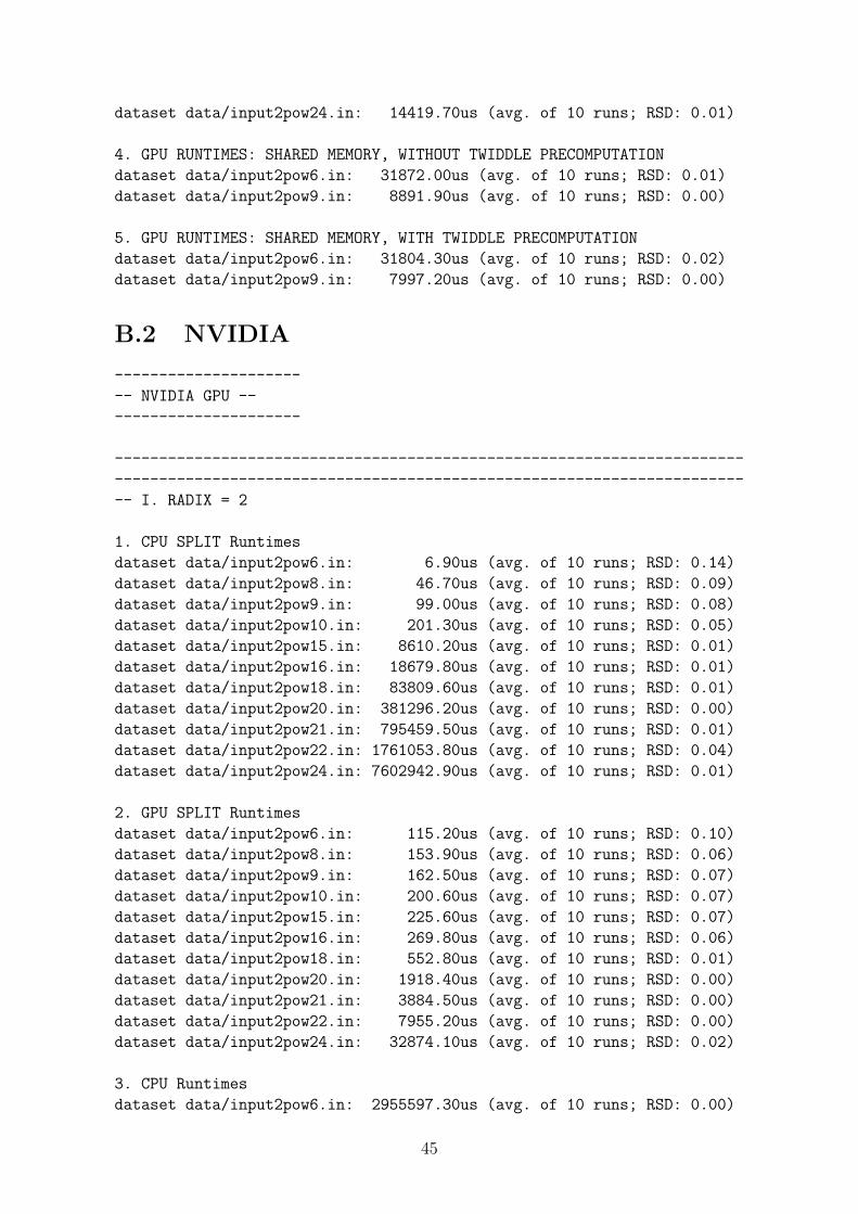
dataset data/input2pow24.in: 14419.70us (avg. of 10 runs; RSD: 0.01)
4. GPU RUNTIMES: SHARED MEMORY, WITHOUT TWIDDLE PRECOMPUTATION
dataset data/input2pow6.in: 31872.00us (avg. of 10 runs; RSD: 0.01)
dataset data/input2pow9.in: 8891.90us (avg. of 10 runs; RSD: 0.00)
5. GPU RUNTIMES: SHARED MEMORY, WITH TWIDDLE PRECOMPUTATION
dataset data/input2pow6.in: 31804.30us (avg. of 10 runs; RSD: 0.02)
dataset data/input2pow9.in: 7997.20us (avg. of 10 runs; RSD: 0.00)
B.2 NVIDIA
---------------------
-- NVIDIA GPU --
---------------------
-----------------------------------------------------------------------
-----------------------------------------------------------------------
-- I. RADIX = 2
1. CPU SPLIT Runtimes
dataset data/input2pow6.in: 6.90us (avg. of 10 runs; RSD: 0.14)
dataset data/input2pow8.in: 46.70us (avg. of 10 runs; RSD: 0.09)
dataset data/input2pow9.in: 99.00us (avg. of 10 runs; RSD: 0.08)
dataset data/input2pow10.in: 201.30us (avg. of 10 runs; RSD: 0.05)
dataset data/input2pow15.in: 8610.20us (avg. of 10 runs; RSD: 0.01)
dataset data/input2pow16.in: 18679.80us (avg. of 10 runs; RSD: 0.01)
dataset data/input2pow18.in: 83809.60us (avg. of 10 runs; RSD: 0.01)
dataset data/input2pow20.in: 381296.20us (avg. of 10 runs; RSD: 0.00)
dataset data/input2pow21.in: 795459.50us (avg. of 10 runs; RSD: 0.01)
dataset data/input2pow22.in: 1761053.80us (avg. of 10 runs; RSD: 0.04)
dataset data/input2pow24.in: 7602942.90us (avg. of 10 runs; RSD: 0.01)
2. GPU SPLIT Runtimes
dataset data/input2pow6.in: 115.20us (avg. of 10 runs; RSD: 0.10)
dataset data/input2pow8.in: 153.90us (avg. of 10 runs; RSD: 0.06)
dataset data/input2pow9.in: 162.50us (avg. of 10 runs; RSD: 0.07)
dataset data/input2pow10.in: 200.60us (avg. of 10 runs; RSD: 0.07)
dataset data/input2pow15.in: 225.60us (avg. of 10 runs; RSD: 0.07)
dataset data/input2pow16.in: 269.80us (avg. of 10 runs; RSD: 0.06)
dataset data/input2pow18.in: 552.80us (avg. of 10 runs; RSD: 0.01)
dataset data/input2pow20.in: 1918.40us (avg. of 10 runs; RSD: 0.00)
dataset data/input2pow21.in: 3884.50us (avg. of 10 runs; RSD: 0.00)
dataset data/input2pow22.in: 7955.20us (avg. of 10 runs; RSD: 0.00)
dataset data/input2pow24.in: 32874.10us (avg. of 10 runs; RSD: 0.02)
3. CPU Runtimes
dataset data/input2pow6.in: 2955597.30us (avg. of 10 runs; RSD: 0.00)
45
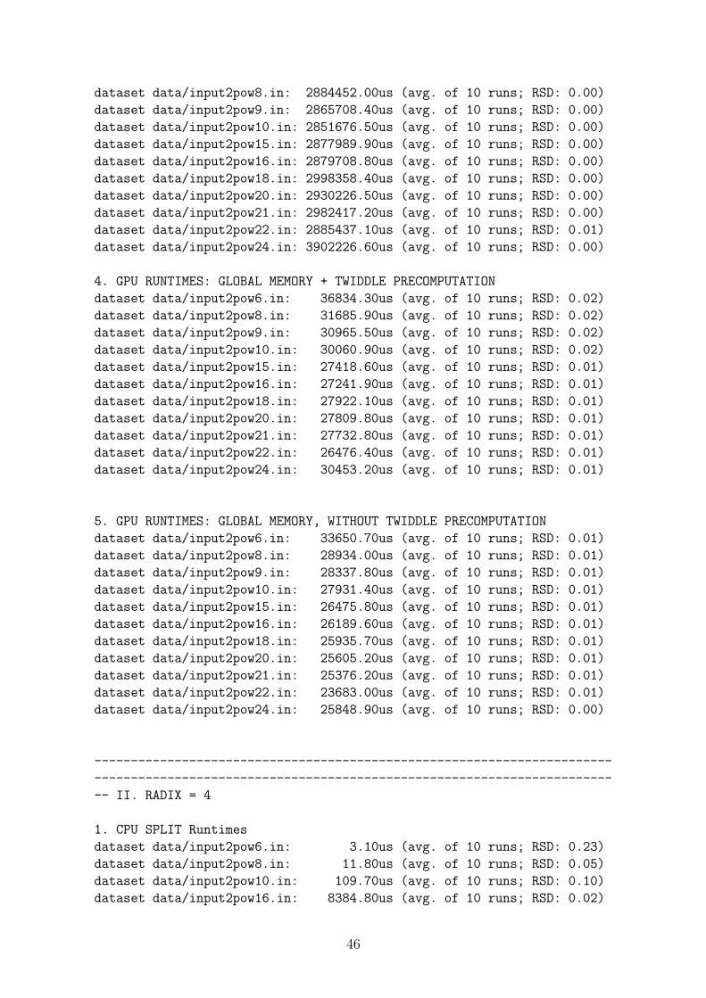
dataset data/input2pow8.in: 2884452.00us (avg. of 10 runs; RSD: 0.00)
dataset data/input2pow9.in: 2865708.40us (avg. of 10 runs; RSD: 0.00)
dataset data/input2pow10.in: 2851676.50us (avg. of 10 runs; RSD: 0.00)
dataset data/input2pow15.in: 2877989.90us (avg. of 10 runs; RSD: 0.00)
dataset data/input2pow16.in: 2879708.80us (avg. of 10 runs; RSD: 0.00)
dataset data/input2pow18.in: 2998358.40us (avg. of 10 runs; RSD: 0.00)
dataset data/input2pow20.in: 2930226.50us (avg. of 10 runs; RSD: 0.00)
dataset data/input2pow21.in: 2982417.20us (avg. of 10 runs; RSD: 0.00)
dataset data/input2pow22.in: 2885437.10us (avg. of 10 runs; RSD: 0.01)
dataset data/input2pow24.in: 3902226.60us (avg. of 10 runs; RSD: 0.00)
4. GPU RUNTIMES: GLOBAL MEMORY + TWIDDLE PRECOMPUTATION
dataset data/input2pow6.in: 36834.30us (avg. of 10 runs; RSD: 0.02)
dataset data/input2pow8.in: 31685.90us (avg. of 10 runs; RSD: 0.02)
dataset data/input2pow9.in: 30965.50us (avg. of 10 runs; RSD: 0.02)
dataset data/input2pow10.in: 30060.90us (avg. of 10 runs; RSD: 0.02)
dataset data/input2pow15.in: 27418.60us (avg. of 10 runs; RSD: 0.01)
dataset data/input2pow16.in: 27241.90us (avg. of 10 runs; RSD: 0.01)
dataset data/input2pow18.in: 27922.10us (avg. of 10 runs; RSD: 0.01)
dataset data/input2pow20.in: 27809.80us (avg. of 10 runs; RSD: 0.01)
dataset data/input2pow21.in: 27732.80us (avg. of 10 runs; RSD: 0.01)
dataset data/input2pow22.in: 26476.40us (avg. of 10 runs; RSD: 0.01)
dataset data/input2pow24.in: 30453.20us (avg. of 10 runs; RSD: 0.01)
5. GPU RUNTIMES: GLOBAL MEMORY, WITHOUT TWIDDLE PRECOMPUTATION
dataset data/input2pow6.in: 33650.70us (avg. of 10 runs; RSD: 0.01)
dataset data/input2pow8.in: 28934.00us (avg. of 10 runs; RSD: 0.01)
dataset data/input2pow9.in: 28337.80us (avg. of 10 runs; RSD: 0.01)
dataset data/input2pow10.in: 27931.40us (avg. of 10 runs; RSD: 0.01)
dataset data/input2pow15.in: 26475.80us (avg. of 10 runs; RSD: 0.01)
dataset data/input2pow16.in: 26189.60us (avg. of 10 runs; RSD: 0.01)
dataset data/input2pow18.in: 25935.70us (avg. of 10 runs; RSD: 0.01)
dataset data/input2pow20.in: 25605.20us (avg. of 10 runs; RSD: 0.01)
dataset data/input2pow21.in: 25376.20us (avg. of 10 runs; RSD: 0.01)
dataset data/input2pow22.in: 23683.00us (avg. of 10 runs; RSD: 0.01)
dataset data/input2pow24.in: 25848.90us (avg. of 10 runs; RSD: 0.00)
-----------------------------------------------------------------------
-----------------------------------------------------------------------
-- II. RADIX = 4
1. CPU SPLIT Runtimes
dataset data/input2pow6.in: 3.10us (avg. of 10 runs; RSD: 0.23)
dataset data/input2pow8.in: 11.80us (avg. of 10 runs; RSD: 0.05)
dataset data/input2pow10.in: 109.70us (avg. of 10 runs; RSD: 0.10)
dataset data/input2pow16.in: 8384.80us (avg. of 10 runs; RSD: 0.02)
46

dataset data/input2pow18.in: 37673.80us (avg. of 10 runs; RSD: 0.02)
dataset data/input2pow20.in: 181204.80us (avg. of 10 runs; RSD: 0.01)
dataset data/input2pow22.in: 791705.00us (avg. of 10 runs; RSD: 0.06)
dataset data/input2pow24.in: 4542222.00us (avg. of 10 runs; RSD: 0.00)
2. GPU SPLIT Runtimes
dataset data/input2pow6.in: 152.50us (avg. of 10 runs; RSD: 0.07)
dataset data/input2pow8.in: 159.90us (avg. of 10 runs; RSD: 0.06)
dataset data/input2pow10.in: 235.00us (avg. of 10 runs; RSD: 0.05)
dataset data/input2pow16.in: 361.60us (avg. of 10 runs; RSD: 0.04)
dataset data/input2pow18.in: 628.10us (avg. of 10 runs; RSD: 0.02)
dataset data/input2pow20.in: 1569.70us (avg. of 10 runs; RSD: 0.01)
dataset data/input2pow22.in: 5627.90us (avg. of 10 runs; RSD: 0.00)
dataset data/input2pow24.in: 22404.70us (avg. of 10 runs; RSD: 0.03)
3. CPU Runtimes
dataset data/input2pow6.in: 1296727.10us (avg. of 10 runs; RSD: 0.00)
dataset data/input2pow8.in: 1213851.40us (avg. of 10 runs; RSD: 0.00)
dataset data/input2pow10.in: 1200030.30us (avg. of 10 runs; RSD: 0.00)
dataset data/input2pow16.in: 1210837.70us (avg. of 10 runs; RSD: 0.00)
dataset data/input2pow18.in: 1433830.80us (avg. of 10 runs; RSD: 0.02)
dataset data/input2pow20.in: 1335269.10us (avg. of 10 runs; RSD: 0.03)
dataset data/input2pow22.in: 1259790.40us (avg. of 10 runs; RSD: 0.05)
dataset data/input2pow24.in: 1751502.20us (avg. of 10 runs; RSD: 0.00)
4. GPU RUNTIMES: GLOBAL MEMORY + TWIDDLE PRECOMPUTATION
dataset data/input2pow6.in: 23920.40us (avg. of 10 runs; RSD: 0.01)
dataset data/input2pow8.in: 18345.80us (avg. of 10 runs; RSD: 0.01)
dataset data/input2pow10.in: 16953.20us (avg. of 10 runs; RSD: 0.01)
dataset data/input2pow16.in: 15182.80us (avg. of 10 runs; RSD: 0.00)
dataset data/input2pow18.in: 15089.70us (avg. of 10 runs; RSD: 0.00)
dataset data/input2pow20.in: 14851.10us (avg. of 10 runs; RSD: 0.01)
dataset data/input2pow22.in: 13831.20us (avg. of 10 runs; RSD: 0.00)
dataset data/input2pow24.in: 15272.70us (avg. of 10 runs; RSD: 0.00)
5. GPU RUNTIMES: GLOBAL MEMORY, WITHOUT TWIDDLE PRECOMPUTATION
dataset data/input2pow6.in: 23383.00us (avg. of 10 runs; RSD: 0.02)
dataset data/input2pow8.in: 18219.20us (avg. of 10 runs; RSD: 0.02)
dataset data/input2pow10.in: 17082.10us (avg. of 10 runs; RSD: 0.01)
dataset data/input2pow16.in: 15300.30us (avg. of 10 runs; RSD: 0.00)
dataset data/input2pow18.in: 15036.40us (avg. of 10 runs; RSD: 0.01)
dataset data/input2pow20.in: 14649.30us (avg. of 10 runs; RSD: 0.01)
dataset data/input2pow22.in: 13483.60us (avg. of 10 runs; RSD: 0.01)
dataset data/input2pow24.in: 14579.40us (avg. of 10 runs; RSD: 0.00)
47

-----------------------------------------------------------------------
-----------------------------------------------------------------------
-- III. RADIX 8
1. CPU SPLIT Runtimes
dataset data/input2pow6.in: 2.20us (avg. of 10 runs; RSD: 0.18)
dataset data/input2pow9.in: 13.70us (avg. of 10 runs; RSD: 0.03)
dataset data/input2pow15.in: 2879.10us (avg. of 10 runs; RSD: 0.03)
dataset data/input2pow18.in: 27023.80us (avg. of 10 runs; RSD: 0.02)
dataset data/input2pow21.in: 257328.70us (avg. of 10 runs; RSD: 0.01)
dataset data/input2pow24.in: 3679618.00us (avg. of 10 runs; RSD: 0.01)
2. GPU SPLIT Runtimes
dataset data/input2pow6.in: 132.40us (avg. of 10 runs; RSD: 0.06)
dataset data/input2pow9.in: 165.10us (avg. of 10 runs; RSD: 0.05)
dataset data/input2pow15.in: 253.40us (avg. of 10 runs; RSD: 0.03)
dataset data/input2pow18.in: 556.90us (avg. of 10 runs; RSD: 0.01)
dataset data/input2pow21.in: 2781.40us (avg. of 10 runs; RSD: 0.01)
dataset data/input2pow24.in: 21521.70us (avg. of 10 runs; RSD: 0.03)
3. CPU Runtimes
dataset data/input2pow6.in: 978961.10us (avg. of 10 runs; RSD: 0.00)
dataset data/input2pow9.in: 871656.50us (avg. of 10 runs; RSD: 0.00)
dataset data/input2pow15.in: 919394.80us (avg. of 10 runs; RSD: 0.00)
dataset data/input2pow18.in: 1338541.40us (avg. of 10 runs; RSD: 0.03)
dataset data/input2pow21.in: 1250893.10us (avg. of 10 runs; RSD: 0.11)
dataset data/input2pow24.in: 1683305.40us (avg. of 10 runs; RSD: 0.00)
4. GPU RUNTIMES: GLOBAL MEMORY + TWIDDLE PRECOMPUTATION
dataset data/input2pow6.in: 27282.40us (avg. of 10 runs; RSD: 0.02)
dataset data/input2pow9.in: 17112.50us (avg. of 10 runs; RSD: 0.02)
dataset data/input2pow15.in: 13330.10us (avg. of 10 runs; RSD: 0.02)
dataset data/input2pow18.in: 12757.30us (avg. of 10 runs; RSD: 0.00)
dataset data/input2pow21.in: 12135.10us (avg. of 10 runs; RSD: 0.00)
dataset data/input2pow24.in: 12084.10us (avg. of 10 runs; RSD: 0.00)
5. GPU RUNTIMES: GLOBAL MEMORY, WITHOUT TWIDDLE PRECOMPUTATION
dataset data/input2pow6.in: 29448.10us (avg. of 10 runs; RSD: 0.03)
dataset data/input2pow9.in: 17185.30us (avg. of 10 runs; RSD: 0.02)
dataset data/input2pow15.in: 13672.60us (avg. of 10 runs; RSD: 0.00)
dataset data/input2pow18.in: 12932.60us (avg. of 10 runs; RSD: 0.00)
dataset data/input2pow21.in: 12266.80us (avg. of 10 runs; RSD: 0.00)
dataset data/input2pow24.in: 12009.90us (avg. of 10 runs; RSD: 0.00)
48

49

Bibliography
[1] John D Owens, David Luebke, Naga Govindaraju, Mark Harris, Jens Kruger,Aaron E Lefohn, and Timothy J Purcell. A survey of general-purpose computationon graphics hardware. In Computer graphics forum, volume 26, pages 80–113,2007.
[2] Naga K. Govindaraju, Brandon Lloyd, Yuri Dotsenko, Burton Smith, and JohnManferdelli. High performance discrete fourier transforms on graphics processors.In Proceedings of the 2008 ACM/IEEE Conference on Supercomputing, SC ’08,pages 2:1–2:12, Piscataway, NJ, USA, 2008. IEEE Press.
[3] Troels Henriksen, Niels G. W. Serup, Martin Elsman, Fritz Henglein, and Cos-min E. Oancea. Futhark: Purely functional gpu-programming with nested paral-lelism and in-place array updates. SIGPLAN Not., 52(6):556–571, June 2017.
[4] James W. Cooley and John W. Tukey. An Algorithm for the Machine Calculationof Complex Fourier Series. Math. Comput., 19:297–301, 1965.
[5] Akira Nukada, Yasuhiko Ogata, Toshio Endo, and Satoshi Matsuoka. Bandwidthintensive 3-d fft kernel for gpus using cuda. In Proceedings of the 2008 ACM/IEEEConference on Supercomputing, SC ’08, pages 5:1–5:11, Piscataway, NJ, USA,2008. IEEE Press.
[6] Matteo Frigo. A fast fourier transform compiler. In Proceedings of the ACM SIG-PLAN 1999 Conference on Programming Language Design and Implementation,PLDI ’99, pages 169–180, New York, NY, USA, 1999. ACM.
[7] David P.H. Jørgensen and Kasper A. Hansen. Bachelor thesis: Fast fourier trans-formation in furthark, January 2018.
[8] Troels Henriksen and Cosmin E. Oancea. Bounds Checking: An Instance ofHybrid Analysis. In Procs. of ACM SIGPLAN Int. Workshop on Libraries, Lan-guages, and Compilers for Array Programming, ARRAY’14, pages 88:88–88:94,New York, NY, USA, 2014. ACM.
[9] Troels Henriksen, Martin Elsman, and Cosmin E. Oancea. Size Slicing: A HybridApproach to Size Inference in Futhark. In Procs. of the 3rd ACM SIGPLANWorkshop on Functional High-performance Computing, FHPC’14, pages 31–42,New York, NY, USA, 2014. ACM.
[10] Troels Henriksen, Martin Dybdal, Henrik Urms, Anna Sofie Kiehn, Daniel Gavin,Hjalte Abelskov, Martin Elsman, and Cosmin Oancea. APL on GPUs: A TAILfrom the Past, Scribbled in Futhark. In Procs. of the 5th Int. Workshop on
50

Functional High-Performance Computing, FHPC’16, pages 38–43, New York, NY,USA, 2016. ACM.
[11] Bernard Legrand. Mastering Dyalog APL. Dyalog Limited, November 2009.
[12] Cosmin E. Oancea and Stephen M. Watt. Domains and expressions: An interfacebetween two approaches to computer algebra. In Proceedings of the 2005 Inter-national Symposium on Symbolic and Algebraic Computation, ISSAC ’05, pages261–268, New York, NY, USA, 2005. ACM.
[13] Y. Chicha, M. Lloyd, C. Oancea, and S. M. Watt. Parametric Polymorphismfor Computer Algebra Software Components. In Proc. 6th International Sympo-sium on Symbolic and Numeric Algorithms for Scientific Comput., pages 119–130.Mirton Publishing House, 2004.
[14] Troels Henriksen, Ken Friis Larsen, and Cosmin E. Oancea. Design and GPGPUPerformance of Futhark’s Redomap Construct. In Procs. of the 3rd ACM SIG-PLAN Int. Workshop on Libraries, Languages, and Compilers for Array Pro-gramming, ARRAY’16, pages 17–24, New York, NY, USA, 2016. ACM.
[15] Rasmus Wriedt Larsen and Troels Henriksen. Strategies for regular segmentedreductions on gpu. In Proceedings of the 6th ACM SIGPLAN International Work-shop on Functional High-Performance Computing, FHPC 2017, pages 42–52, NewYork, NY, USA, 2017. ACM.
[16] Cosmin E. Oancea, Christian Andreetta, Jost Berthold, Alain Frisch, and FritzHenglein. Financial Software on GPUs: Between Haskell and Fortran. In Pro-ceedings of the 1st ACM SIGPLAN Workshop on Functional High-performanceComputing, FHPC ’12, pages 61–72, New York, NY, USA, 2012. ACM.
[17] D. Sundararajan. The Discrete Fourier Transform: Theory, Algorithms and Ap-plications. World Scientific, 2001.
[18] W. T. Cochran, J. W. Cooley, D. L. Favin, H. D. Helms, R. A. Kaenel, W. W.Lang, G. C. Maling, D. E. Nelson, C. M. Rader, and P. D. Welch. What is thefast fourier transform? Proceedings of the IEEE, 55(10):1664–1674, Oct 1967.
51