DESIGNING AN ONLINE CONTROLLER FOR

TEMPERATURE MEASUREMENT

By

SY ARIF AH AZIZA KAMALIA BINTI SYED F ARUK

FINAL PROJECT REPORT

Submitted to the Electrical & Electronics Engineering Programme in Partial Fulfillment of the Requirements

for the Degree

Bachelor of Engineering (Hons) (Electrical & Electronics Engineering)

Universiti Teknologi Petronas

Bandar Seri Iskandar

31750 Tronoh

Perak Darul Ridzuan

© Copyright 2009

by

Syarifah Aziza Kamalia Binti Syed Faruk, 2009

ii

Approved:

CERTIFICATION OF APPROVAL

DESIGNING AN ONLINE CONTROLLER FOR

TEMPERATURE MEASUREMENT

by

Syarifah Aziza Kamalia Binti Syed Faruk

A project dissertation submitted to the

Electrical & Electronics Engineering Programme Universiti Teknologi PETRONAS

in partial fulfilment of the requirement for the Bachelor of Engineering (Hons)

(Electrical & Electronics Engineering)

~;:::;;:::::::::===- SDr Taj Mohammad Baloch enlor Lecturer

Electrical & Electronic E .

- -1---1-L_----""F,.. ~u::_:__·· ·I-'~,_:_·'1-~Go-P3Universitl Tekno/ogi PE;~·~~~'s"g ~ ) 1750 Tronoh

aj Mohammad. Baloch Perak Daru/ Rldzuan, MALAYSIA

Project Supervisor

UNIVERSITI TEKNOLOGI PETRONAS

TRONOH. PERAK

December 2009

iii

CERTIFICATION OF ORIGINALITY

This is to certify that I am responsible for the work submitted in this project, that the

original work is my own except as specified in the references and acknowledgements,

and that the original work contained herein have not been undertaken or done by

unspecified sources or persons.

~-· Syarifah Aziza Kamalia Binti Syed Faruk

iv

ABSTRACT

This document reports the progress of the project so far in detail. Here the task

done is clearly laid out. Problems encountered were identified and listed. The

solutions for each problem were developed as fmalizing the design continues.

Considering the problems that might arise while completing the project, preventions

of such problems are planed. All the future work was scheduled specifically to

fabricate the final design chosen. In recent years, the application of controller for

measurement based techniques to a wide range of industrial processes has become

increasingly common. One reason for this development is the level of development of

theory of measurement and its implementation into application tools for feasible use.

Controller for measurement is the success of automatic process control, real­

monitoring, and a long term performance tracking in improving plant performances

depends crucially on measurement. In the oil and gas industry, due to high

dissemination levels of many production fields and the complex nature of processes,

the need for increased efficiencies and highly effective processing of a large amount

of information is particularly evident. Therefore, controller for measurement has been

introduced as a plan to contract with indecisive, inexact or qualitative decision

making problem. Controllers that unite intelligent and conservative techniques are

frequently used in the intelligent control of complex dynamic systems. As a result, the

controller can be used to advance on hand conventional control systems in

conjunction with an extra level of intelligence to existing control technique to make it

more efficient.

v

ACKNOWLEDGEMENTS

Alhamdulillah, in the name of Allah, Most Gracious and Most Merciful, thank

God for His blessings and guidance, at last the author has successfully finished the

first part of Final Year Project I. Above all, we would like to express our gratitude to

my supervisor, Dr Taj Mohammad Baloch for the supervision and guidance

throughout this project. I appreciate their effort in providing advice, great support and

assistance that enable this project to achieve its objectives and be completed

successfully within the time frame given.

I would like to acknowledge other Electrical Electronic Engineering lecturers

in sharing their expertise in various plant design aspects. With this opportunity, I am

able to deepen our knowledge, both in theory and practical in the basic of a design an

online controller for temperature measurement.

I would like to my deepest appreciation to my course mates especially Mr

Azri Hafiz in exchanging ideas and provide guidance in unfamiliar design

characteristics and usage of plant design software.

Lastly but not the least, we would like to show our heartfelt gratitude our

family and friends and those who has directly or indirectly involved in this project,

for their tremendous support and motivation during undertaking this project.

vi

TABLE OF CONTENTS

LIST OF TABLES ....................................................................................................... ix

LIST OF FIGURES ...................................................................................................... x

LIST OF ABBREVIATIONS ...................................................................................... xi

CHAPTER I ................................................................................................................. !

1.1 Introduction ...................................................................................... I

1.2 Problem Statement ........................................................................... 2

1.3 Process Control Algorithm ............................................................... 2

CHAPTER2 ................................................................................................................. 3

2.1 Literature Review ............................................................................. 3

2.2 The Workhorses ............................................................................... 5

2.2.1 Thermocouple .......................................................................... 5

222 Resistive Temperature Devices ............................................... 7

2.2.3 Thermistors .............................................................................. 8

2.2.4 Infrared sensors ........................................................................ 9

CHAPTER 3 ............................................................................................................... 11

3 .I Procedure ........................................................................................ 11

3.2 Tool Required ................................................................................. 12

CHAPTER 4 ............................................................................................................... 13

4.1 Circuit Operation ............................................................................ l3

4.1.1 Transmitter circuit operation ................................................. 14

4.1.2 Receiver circuit operation ..................................................... 15

4.2 Modification on Circuit Operation ................................................. 13

4.2.1 Transmitter circuit operation ................................................. 14

4.2.2 Receiver circuit operation ..................................................... 14

4.3 Experiment of Accuracy Comparison ............................................ 13

CHAPTER 5 ............................................................................................................... 20

5 .I Introduction .................................................................................... 20

5.2 Recommendation And Future Work Plan ...................................... 20

5.3 Conclusion ...................................................................................... 21

REFERENCES ............................................................................................................ 22

vii

APPENDICES ............................................................................................................ 23

Appendix A Parts in Circuit.. ............................................................... 24

Appendix B Precision Voltage to Frequency Converters .................... 26

Appendix C Precision Centrigade Temperature Sensors ..................... 33

Appendix D Quad 2 Input Schmitt Nand Gate .................................... 39

viii

LIST OF TABLES

Table 1: Medium of measurement is boiled water ........................................ .l8

Table 2: Medium of measurement is lukewarm water .................................... 19

Table 3: Medium of measurement is ice .................................................... 34

Table 4: Ordering Information ................................................................ 26

Table 5: Electrical Characteristics for LM331 ........................................................... 28

Table 6: Electrical Characteristics for LM35 ............................................................. 34

Table 7: Absolute Maximum Rating for NAND Gate ............................................... 38

ix

LIST OF FIGURES

Figure I: Simple Circuit on Temperature Controller ................................................... 3

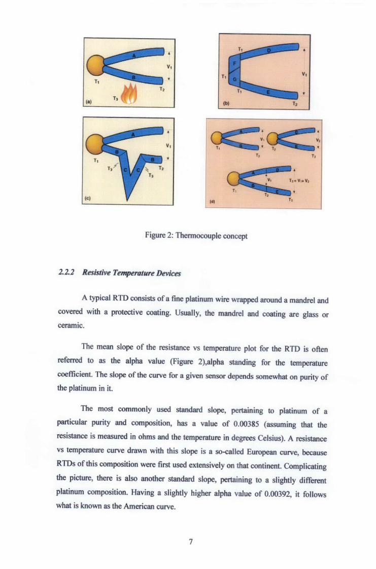
Figure 2: Thermocouple concept ............................ ! ................................................... 7

Figure 3: Resistance temperature relationship of a thermistor .................................... 8

Figure 4: Resistance temperature relationship of a thermistor .................................... 8

Figure 5: Thermistor Sensor .................................... : ................................................... 9

Figure 6: Methodology Flowchart ............................................................................ 12 '

Figure 7: Transmitter Circuit ..................................................................................... 13

Figure 8: Receiver Circuit ........................................ ; ................................................. 14

Figure 9: Circuit Operation when LM35 touched ice and hot water ........................ 15

Figure 10: Transmitter (433MHz) ............................................................ 16

Figure 11: RF transmitter module CS90 1 ................................................... 16

Figure 12: RF receiver module CS902 ................ 1

•••••••••••••••••••••••••••••••••••••• 17

Figure 13: Transmitter and Receiver Circuit .............................................. 17

Figure 14: Comparison between the prototype and' alcohol thermometer as reference temperature ............................................... , ..................................... .19

X

LIST OF ABBREVIATIONS

RID Resistive Temperature Device

T Temperature

IC Integrated Circuit

Q Transistor

xi

CHAPTER!

INTRODUCTION

1.1 Introduction

Human progress from a primitive state to our present complex, technological

world has been marked by learning new and improved methods to control the

environment. The term control means methods to force parameters in the environment

to have specific values. This can be as simple as making the temperature in a room

stay some certain value or as complex as manufacturing an integrated circuit or

guiding a spacecraft to other planets in the galaxy.

When the value of a variable is needed, it can be obtained from at least two real­

time methods. First, it can be measured "directly" by a sensor; as an example, a

temperature can be measured by a thermocouple, although the actual value sensed is

the voltage generated for a bimetallic connection with nodes at two temperature; the

references and proeess temperatures.

This sensor is called direct sensor because the physical principle underlying the

measurement is independent of the process application and the relationship between

the sensor signal and process variable is level, pressure, temperature, and flows of

many fluids. Also, the compositions and physical properties of some process streams

can be determined in real-time with on-stream analyzers.

In the second method, the variable cannot be measured, at least at reasonable

cost, in real-time, but it can be inferred using other measurement and a process­

specific correlation.

Not all variables can be measured in real time. These variables have to be

determined through analysis of sample material. When the sample and analysis can be

performed quickly the value can be used in feedback control. These are many

industrial examples of controllers that use results and are executed every few hours.

I

While not providing control performances as good as would be possible with on­

stream analysis, this approach usually gives much better performances that not using

lab value.

1.2 Problem Statement

Many problems encountered in designing the controller which include this process:

• To develop the actual circuit both for transmitter and receiver.

• To encounter with the complexity of receiver circuit.

• To design circuit for the mathematical model and simulation model.

1.3 Process Control Algorithm

The process control algorithm undertakes the following procedure:

I. Measurement of a certain output based on the sensors input to the controller

2. Controller decision on the required state.

3. Output signal to the plant from the controller, manipulating the process.

4. Plant process operation based on the controller's decision.

2

CHAPTER2

LITERATURE REVIEW

2.1 Literature Review

The control system for modem industrial plants typically includes thousands

of individual control loops. During control system design, preliminary controller

settin~ are specified based on process knowledge, control objectives and prior

experience. After a controller is installed, the prelimiuary setting often to be

satisfactory but for critical control loops, the preliminary settings may have to be

adjusted in order to achieve satisfactory control. This is called online controller.

Online controller tuning involves plant testing, often on a trial and error basis,

the tuning can be quite tedious and time consuming. Consequently, good initial

controller settings are very desirable to reduce the required time and etfurt. Ideally,

the preliminary settings from the control system design can be used as the initial field

settings. If the preliminary settings are not satisfactory, alternative settings can be

obtained from simple experiment tests. If necessary, the settings can be fine tuned by

a modest amount of trial and error.

Fh-)·~v fd-;.te-nr 1

. .-T--"---"----,

Figure I: Simple Circuit on Temperature Controller

3

Temperature can be measured via a diverse array of sensors. All of them infer

temperature by sensing some change in a physical characteristic. Six types with

which the engineer is likely to come into contact are: thermocouples, resistive

temperature devices (RTDs and thermistors), infrared radiators, bimetallic devices,

liquid expansion devices, and change-of-state devices.

Thermocouples consist essentially of two strips or wires made of different

metals and joined at one end. As discussed later, changes in the temperature at that

juncture induce a change in electromotive force (emf) between the other ends. As

temperature goes up, this output (emf) of the thermocouple rises, though not

necessarily linearly.

Resistive temperature devices capitalize on the fact that the electrical

resistance of a material changes as its temperature changes. Two key types are the

metallic devices (commonly referred to as RTDs), and thermistors. As their name

indicates, RTDs rely on resistance change in a metal, with the resistance rising more

or less linearly with temperature. Thermistors are based on resistance change in a

ceramic semiconductor; the resistance drops nonlinearly with temperature rise.

Infrared sensors are no contacting devices. They infer temperature by

measuring the thermal radiation emitted by a material.

Bimetallic devices take advantage of the difference in rate of thermal

expansion between different metals. Strips of two metals are bonded together. When

heated, one side will expand more than the other, and the resulting bending is

translated into a temperature reading by mechanical linkage to a pointer. These

devices are portable and they do not require a power supply, but they are usually not

as accurate as thermocouples or RIDs and they do not readily lend themselves to

temperature recording.

Fluid-expansion devices, typified by the household thermometer, generally

come in two main classifications: the mercury type and the organic-liquid type.

Versions employing gas instead of liquid are also available. Mercury is considered an

environmental hazard, so there are regulations governing the shipment of devices that

contain it. Fluid-expansion sensors do not require electric power, do not pose

explosion hazards, and are stable even after repeated cycling. On the other hand, they

4

do not generate data that are easily recorded or transmitted, and they cannot make

spot or point measurements.

Change-of-state temperature sensors consist of labels, pellets, crayons,

lacquers or liquid crystals whose appearance changes once a certain temperature is

reached. They are used, for instance, with steam traps - when a trap exceeds a certain

temperature, a white dot on a sensor label attached to the trap will turn black.

Response time typically takes minutes, so these devices often do not respond to

transient temperature changes. And accuracy is lower than with other types of

sensors. Furthermore, the change in state is irreversible, except in the case of liquid­

crystal displays. Even so, change-of-state sensors can be handy when one needs

confirmation that the temperature of a piece of equipment or a material has not

exceeded a certain level, for instance for technical or legal reasons during product

shipment.

2.2 The Workhorses

In the chemical process industries, the most commonly used temperature

sensors are thermocouples, resistive devices and infrared devices. There is

widespread misunderstanding as to how these devices work and how they should be

used.

2.2.1 Thermocouple

Consider first the thermocouple, probably the most-often-used and least­

understood of the three. Essentially, a thermocouple consists of two alloys joined

together at one end and open at the other. The ( emt) at the output end (the open end;

VI in Figure 2a) is a function of the temperature T1 at the closed end. As the

temperature rises, the emf goes up.

Often the thermocouple is located inside a metal or ceramic shield that

protects it from a variety of enviromnents. Metal-sheathed thermocouples are also

available with many types of outer coatings, such as polytetrafluoroethylene, for

trouble-free use in corrosive solutions.

5

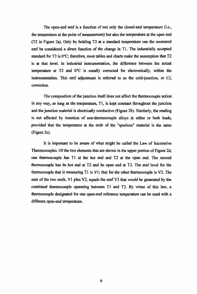
The open-end emf is a function of not only the closed-end temperature (i.e.,

the temperature at the point of measurement) but also the temperature at the open end

(T2 in Figure 2a). Only by holding T2 at a standard temperature can the measured

emf be considered a direct function of the change in Tl. The industrially accepted

standard for T2 is 0°C; therefore, most tables and charts make the assumption that T2

is at that level. In industrial instrumentation, the difference between the actual

temperature at T2 and 0°C is usually corrected for electronically, within the

instrumentation. This emf adjustment is referred to as the cold-junction, or CJ,

correction.

The composition of the junction itself does not affect the thermocouple action

in any way, so long as the temperature, Tl, is kept constant throughout the junction

and the junction material is electrically conductive (Figure 2b). Similarly, the reading

is not affected by insertion of non-thermocouple alloys in either or both leads,

provided that the temperature at the ends of the "spurious" material is the same

(Figure 2c ).

It is important to be aware of what might be called the Law of Successive

Thermocouples. Of the two elements that are shown in the upper portion of Figure 2d,

one thermocouple has Tl at the hot end and T2 at the open end. The second

thermocouple has its hot end at T2 and its open end at T3. The emf level for the

thermocouple that is measuring Tl is VI; that for the other thermocouple is V2. The

sum of the two emfs, VI plus V2, equals the emfV3 that would be generated by the

combined thermocouple operating between Tl and T3. By virtue of this law, a

thermocouple designated for one open-end reference temperature can be used with a

different open-end temperature.

6

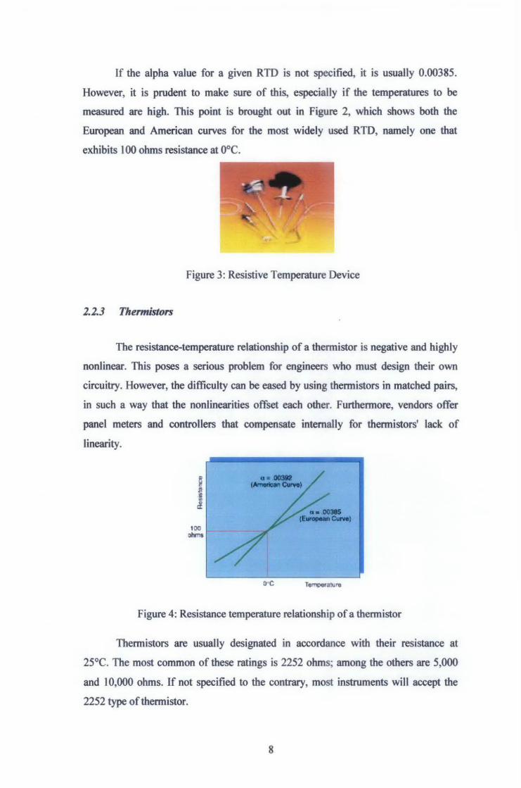
If the alpha value for a given RID is not specified, it is usually 0.00385.

However, it is prudent to make sure of this, especially if the temperatures to be

measured are high. This point is brought out in Figure 2, which shows both the

European and American curves for the most widely used RTD, namely one that

exhibits 100 ohms resistance at 0°C.

Figure 3: Resistive Temperature Device

1.1.3 Thermistors

The resistance-temperature relationship of a thermistor is negative and highly

nonlinear. This poses a serious problem for engineers who must design their own

circuitry. However, the difficulty can be eased by using thermistors in matched pairs,

in such a way that the nonJinearities offset each other. Furthermore, vendors offer

panel meters and controllers that compensate intemaUy for thennistors' lack of

linearity.

10Q ohms

OC Te~l\>re

Figure 4: Resistance temperature relationship of a thermistor

Thermistors are usually designated in accordance with their resistance at

25°C. The most common of these ratings is 2252 ohms; among the others are 5,000

and J 0,000 ohms. If not specified to the contrary, most instruments will accept the

2252 type of thermistor.

8

Figure 5: Thermistor Sensor

1.1.4 Infrared sensors

These measure the amount of radiation emitted by a surface. Electromagnetic

energy radiates from all matter regardless of its temperature. In many process

situations, the energy is in the infrared region. As the temperature goes up, the

amount of infrared radiation and its average frequency go up.

Different materials radiate at different levels of efficiency. This efficiency is

quantified as emissivity, a decimal number or percentage ranging between 0 and 1 or

00/o and 1 00%. Most organic materials, including skin, are very efficient, frequently

exhibiting emissivities of 0.95. Most polished metals, on the other hand, tend to be

inefficient radiators at room temperature, with emissivity or efficiency often 200/o or

less.

To function properly, an infrared measurement device must take into account

the emissivity of the surface being measured. This can often be looked up in a

reference table. However, bear in mind that tables cannot account for localized

conditions such as oxidation and surface roughness. A sometimes practical way to

measure temperature with infrared when the emissivity level is not known is to

"force" the emissivity to a known level, by covering the surface with masking tape

(emissivity of95%) or a highly emissive paint.

Some of the sensor input may well consist of energy that is not emitted by the

equipment or material whose surface is being targeted, but instead is being reflected

by that surface from other equipment or material. Emissivity pertains to energy

radiating from a surface whereas reflection pertains to energy reflected from another

source. Emissivity of an opaque material is an inverse indicator of its reflectivity D

substances that are good emitters do not reflect much incident energy, and thus do not

9

pose much of a problem to the sensor in determining surface temperatures.

Conversely, when one measures a target surface with only, say, 20% emissivity,

much of the energy reaching the sensor might be due to reflection from, e.g., a nearby

furnace at some other temperature. In short, be wary of hot, spurious reflected targets.

An infrared device is like a camera, and thus covers a certain field of view. It

might, for instance, be able to "see" a 1-deg visual cone or a I 00-deg cone. When

measuring a surface, be sure that the surface completely fills the field of view. If the

target surface does not at first fill the field of view, move closer, or use an instrument

with a narrower field of view. Or, simply take the background temperature into

account (i.e., to adjust for it) when reading the instrument.

10

CHAPTER3

METHODOLOGY AND PROJECT WORK

3.1 Procedure Identification

This project is a two semester project. The first half of the project is to

understand the controller and the second half is to design circuit. The complete

project planning is as figure below. The first thing to do is to fmd the specification of

the controller. This required student to study from many source to find the correct

specification. Next is to design the circuit and capture the schematic. Lastly is circuit

validation before proceed to layout design.

Second half of the project starts with design of actual circuit and also the

simulation in the Pspice.

11

Figure 6: Methodology Flowchart

3.2 Tool Required

This project is simulation based only. The software that will be used for

design circuit and layout is Pspice design software and MultiSim Software ..

12

-

CHAPTER4

RESULTS AND DISCUSSION

4.1 Circuit Operation

This circuit is intended for precision centigrade temperature measurement,

with a transmitter section converting to frequency the sensor's output voltage, which

is proportional to the measured temperature. The output frequency bursts are

conveyed into the mains supply cables.

The receiver section counts the signal coming from mains supply and shows

the counting on three 7-segment LED displays. The least significant digit displays

tenths of degree and then a 00.0 to 99.9 oc range is obtained. Transmitter-receiver

distance can reach hundred meters, provided both units are connected to the mains

supply within the control of the same light-meter.

OUT IN IC3

C1r l!6 1!7

t~ 8 5 7

IC2 3

CB

-

Q2 '1'1..1

- -

- -

Figure 7: Transmitter Circuit

13

D4

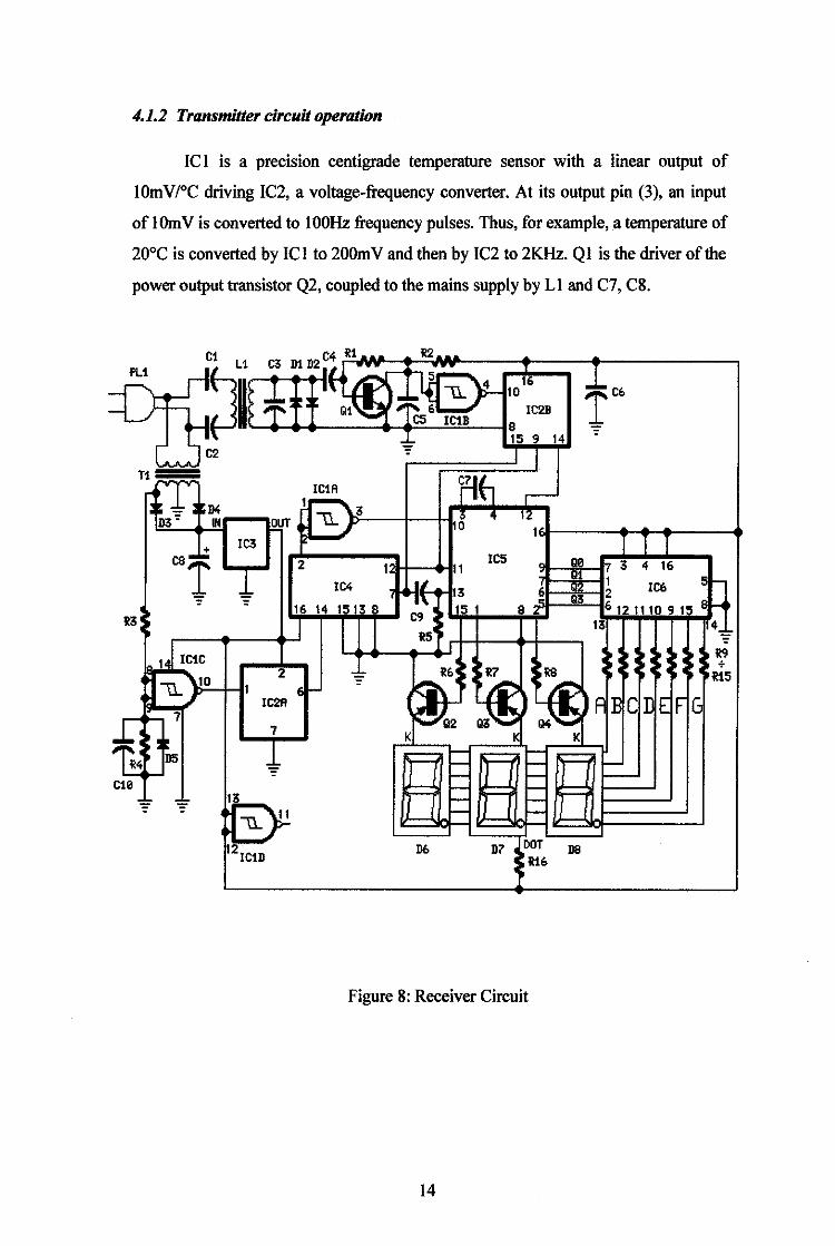
4.1.2 Transmitter circuit operation

IC 1 is a precision centigrade temperature sensor with a linear output of

1Om V /°C driving IC2, a voltage-frequency converter. At its output pin (3), an input

of IOmV is converted to lOOHz frequency pulses. Thus, for example, a temperature of

20°C is converted by IC 1 to 200m V and then by IC2 to 2KHz. Q I is the driver of the

power output transistor Q2, coupled to the mains supply by L1 and C7, C8.

~• ~" a •~01 1 ~ tC6

---4 5 16 ... I' \l.. 4 10 DQ;l: I " "' !<g'"'-li,. <W C5 IC1B 8

[ ..!:- 15 9 14 C2 ~ I I

n=== fiE-! ~ll

IC1A ,-FD4 1r;'"\.3

·~ 4 12 1)3" IN OUT \l..f 1

C8f IC3 T

ICS ll0 2 1 1 3 4 16

t .I/ 1 1 sr-IC4 3 6 2 IC6 .. , Q3

16 14 1513 8 15 1 8 6 12 111 1 r-< 13

I C9

13 \· R5

Jtctc i9 : : +

\l.. '"10 2 "'= i6 i7 R8 115

1 IC2A E - ~~ ~~ )~ f AE CI IE F It: - .... 7

7 ;:::: l~.

K Ki K

t t -'

-R4 D5 - - r-

cte .... - - r--- .,_, - .,_, ¥ "'€" 11--. h - -

1\l.. 11 - -

C1 C4 it R2

2IC1D

D6 D7 DOT D8 116

Figure 8: Receiver Circuit

14

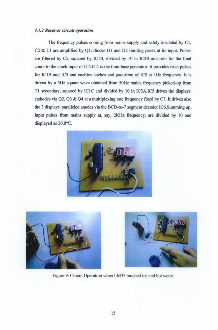
4.1.2 Receiver circuit operation

The frequency pulses coming from mains supply and safely insulated by Cl,

C2 & Ll are amplified by Ql ; diodes 01 and 02 limiting peaks at its input. Pulses

are filtered by C5, squared by ICIB, divided by 10 in IC2B and sent for the fmal

count to the clock input of IC5.IC4 is the time-base generator: it provides reset pulses

for IClB and IC5 and enables latches and gate-time of IC5 at 1Hz frequency. It is

driven by a 5Hz square wave obtained from 50Hz mains frequency picked-up from

Tl secondary, squared by ICIC and divided by 10 in IC2A.IC5 drives the displays'

cathodes via Q2, Q3 & Q4 at a multiplexing rate frequency fixed by C7. It drives also

the 3 displays' paralleled anodes via the BCD-to-7 segment decoder IC6.Summing up,

input pulses from mains supply at, say, 2KHz frequency, are divided by 10 and

displayed as 20.0°C.

Figure 9: Circuit Operation when LM35 touched ice and hot water

15

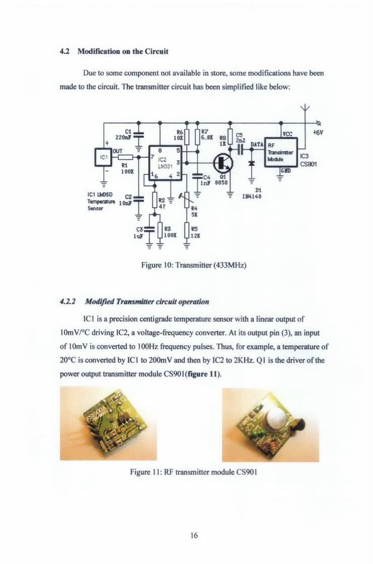
4.2 Modification on tbe Circuit

Due to some component not available in store, some modifications have been

made to the circuit The transmitter circuit has been simplified like below:

DiU RF Transimtter ~

D1 Ill4148

Figure I 0: Transmitter ( 433MHz)

4.2.2 Modifred Transmitter circuit operation

IC1 is a precision centigrade temperature sensor with a linear output of

10mV/°C driving IC2, a voltage-frequency converter. At its output pin (3), an input

of 1Om V is converted to 1OOHz frequency pulses. Thus, for example, a temperature of

20°C is converted by IC 1 to 200m V and then by I C2 to 2KHz. Q 1 is the driver of the

power output transmitter module CS90 I (fagure 11 ).

Figure 11: RF transmitter module CS901

16

4.2.2 Modified Receiver circuit operation

Instead of putting the main supply to produce the frequency, we bad the

frequency pulses coming out from RF receiver module CS902 (fagure 12)

Figure 12: RF receiver module CS902

Figure 13: Transmitter and Receiver Circuit

17

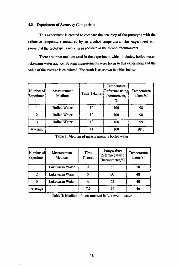
4.3 Experiment of Accuracy Comparison

This experiment is created to compare the accuracy of the prototype with the

reference temperature measured by an alcohol temperature. This experiment will

prove that the prototype is working as accurate as the alcohol thermometer.

There are three medium used in the experiment which includes, boiled water,

lukewarm water and ice. Several measurements were taken in this experiment and the

value of the average is calculated. The result is as shown in tables below:

Temperature Number of Measurement

Time Taken,s Reference using Temperature

!Experimen Medium thermometer, taken,°C oc

1 Boiled Water 10 100 98

2 Boiled Water 12 100 98

3 Boiled Water 12 100 99

Average 11 100 98.5

Table 1: Medium of measurement is boiled water

Number of Measurement Time Temperature

Temperature Experimen Medium Taken,s

Reference using taken,°C

Thermometer, °C

1 Lukewarm Water 8 55 50

2 Lukewarm Water 9 60 48

3 Lukewarm Water 6 62 40

Average 7.6 59 46

Table 2: Medium of measurement is Lukewarm water

18

Number of Measurement Time Temperature

Temperature Reference using

[Experimen Medium Taken,s thermometer, oc taken,°C

1 Ice ll 8.4 11.4

2 Ice 12 11.8 11.3

3 Ice 12 9.8 11.3

Average 11.7 10.0 11.35

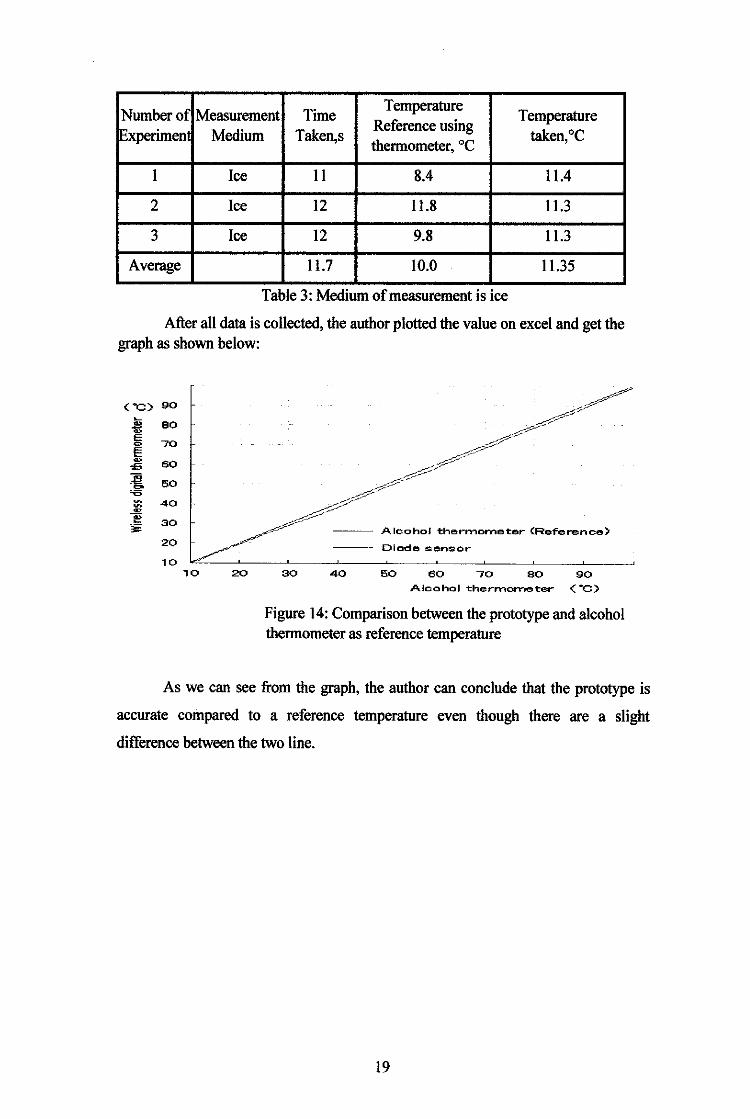
Table 3: Medium of measurement is ice

After all data is collected, the author plotted the value on excel and get the graph as shown below:

("C) 90 ~

~ 80 E 0 70 E ~ 60 £;

.-!:! 60 ~

'6 ~ 40 ~

-"' e 30 .,.. 20

10 10 20 30

-- Alcohol thert'rlorneter (Ref'erence)

-- Diode sensor

40 60 60 70 80 A leo hoi the rrrtorne ter

90 ("C)

Figure 14: Comparison between the prototype and alcohol thermometer as reference temperature

As we can see from the graph, the author can conclude that the prototype is

accurate compared to a reference temperature even though there are a slight

difference between the two line.

19

CHAPTERS

RECOMMENDATION AND CONCLUSION

5.1 Introduction

For this final part of the report, the author had included the suggested

recommendation and future work plan with respect to the project and also necessary

expansion and continuation for the upcoming work. Lastly the report will finished off

with the conclusion, summarizing all relevance information within this project.

5.2 Recommendation and Future Work Plan

So far to the author's observation, there are few recommendation can be made

to ensure a better outcome towards this project. So far it was a great success to finally

do the actual circuit even though both circuits is complex and while there will

definitely be future plan to fmish this projects, below are some recommendation(s)

that can be made:

• To replace the bread board with permanent board.

• To create a workpiece box to put the circuit inside so that it will appear

presentable for the exhibition.

As for the future work plan, the author will be looking to continue the progress

which will commence within the next left months. Future work plans for this project

includes:

1. To experiment the circuit by using a set of a parameters with

temperature variable.

2. To collect the data in the experiment.

20

5.3 Conclusion

These days, many accidents happened in the plant and in high risk area on

platform, factory and etc. Online controller help persona for example engineers and

technicians to record the measurement without having to go to the high risk and

dangerous places. This project have two part to accomplish which is part I is the

simulation of the Temperature Measurement controller circuit. Meanwhile, part 2 is

the development of the circuit of both Transmitter and Receiver circuit. By referring

to project flow, this project progress is smooth as plan. Out of that, other task that can

be done is to improve understanding on design knowledge and other technique of

design.

21

APPENDICES

23

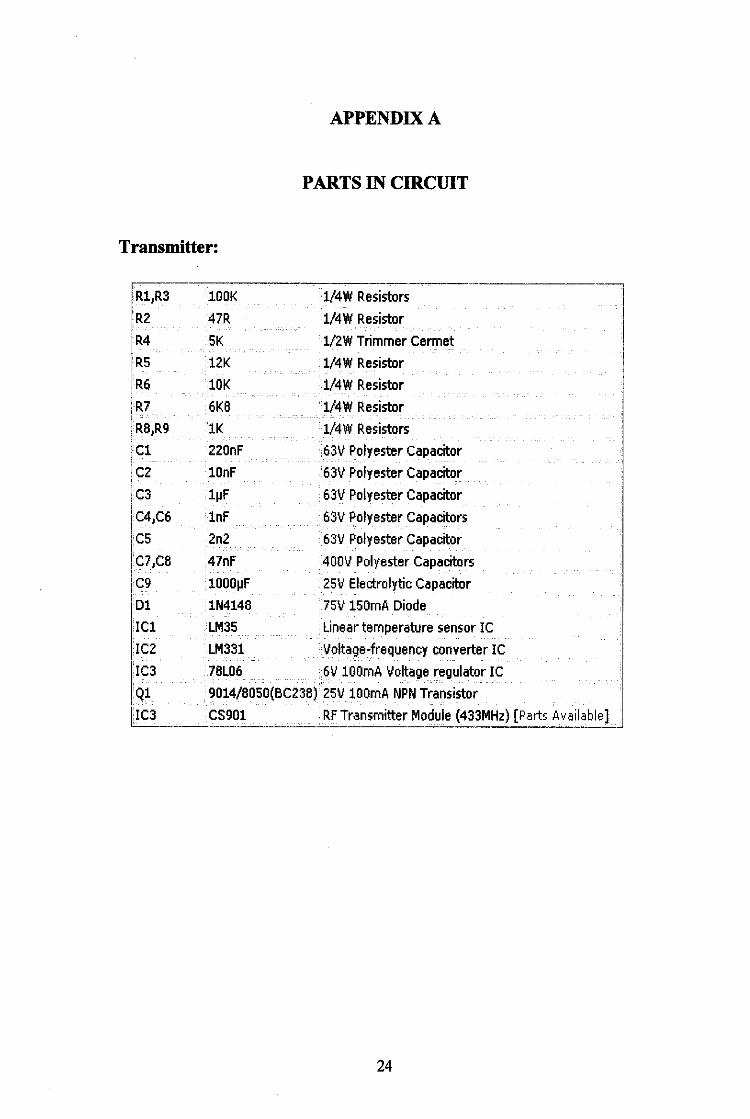
APPENDIX A

PARTS IN CIRCIDT

Transmitter:

R1,R3 lOOK 1/4 W Resistors R2 47R 1/4 W Resistor R4 5K 1/2W Trimmer Cermet R5 12K 1/4 W Resistor R6 lOK 1/4 W Resistor R7 6K8 1/4 W Resistor R8,R9 lK 1/4 W Resistors C1 220nF 63V Polyester Capacitor

C2 lOnF 63V Polyester Capacitor

C3 l~F 63V Polyester Capacitor

C4,C6 lnF 63V Polyester Capacitors

C5 2n2 63V Polyester Capacitor

C7,C8 47nF 400V Polyester Capacitors C9 1000~F 25V Electrolytic Capacitor Dl 1N4148 75V 150mA Diode ICl LM35 . Linear temperature sensor IC

IC2 LM331 Voltage-frequency converter IC

IC3 78L06 6V lOOmA Voltage regulator IC Ql 9014/8050(BC238) 25V lOOmA NPN Transistor

IC3 CS901 RF Transmitter Module (433MHz) [Parts Available]

24

Receiver:

IRl,R2,R4,R5,R6Il2K 1114 W Resistor IR3 I47K lt/4W Resistor IR7·Rl3,Rl4 lzzoR lt/4W Resistors

lcl,C2,C6, lzzonF I63V Polyester Capacitors

lc3 ltnf I63V Polyester Capacitors

lc4 ltoopF I63V Polyester Capacitor

ics I100~F I63V Polyester Capacitors

ID1,D2, I1N4002 I100V lA Diodes

ID3 I1N4148 I75V 150mA Diodes

ID6·DS Iilli !common-cathode 7-segment LED mini-displays

II CO lcsgoz IRF receiver Module [Parts Available]

IICl lcD4093 IQuad 2 input Schmitt NAND Gate IC

IIC2 lcD4sta !Dual BCD Up-Counter IC

IIC3 l7su2 I12V lOOmA Voltage regulator IC

IIC4 lcD4017 !Decade Counter with 10 decoded outputs IC

lies lcD4553 !Three-digit BCD Counter IC

IIC6 lcD4511 IBCD·to·7·Segment Latch/Decoder/Driver IC lqz-Q4 issso(BC327) I45V 800mA PNP Transistors

In jfower transformer

lf200V Primary,12+12V Secondary 3VA Mains transformer

25

APPENDIXB

PRECISION VOLTAGE-TO-FREQUENCY

CONVERTERS

General Description

The LM231/LM33l family of voltage-to-frequency converters is ideally

suited for use in simple low-cost circuits for analog-to-digital conversion, precision

frequency-to-voltage conversion, long-term integration, linear frequency modulation

or demodulation, and many other functions. The output when used as a voltage-to­

frequency converter is a pulse train at a frequency precisely proportional to the

applied input voltage. Thus, it provides all the inherent advantages of the voltage-to­

frequency conversion techniques, and is easy to apply in all standard voltage-to­

frequency converter applications.

Further, the LM231AILM33IA attain a new high level of accuracy versus

temperature which could only be attained with expensive voltage-to-frequency

modules. Additionally the LM231/331 are ideally suited for use in digital systems at

low power supply voltages and can provide low-cost analog-to-digital conversion in

microprocessor controlled systems. And, the frequency from a battery powered

voltage-to-frequency converter can be easily channeled through a simple photo

isolator to provide isolation against high common mode levels.

The LM23l!LM331 utilize a new temperature-compensated band-gap

reference circuit, to provide excellent accuracy over the full operating temperature

range, at power supplies as low as 4.0V. The precision timer circuit has low bias

currents without degrading the quick response necessary for 100 kHz voltage-to­

frequency conversion. And the output are capable of driving 3 TTL loads, or a high

voltage output up to 40V, yet is short-circuit-proof against vee.

26

Features

• Guaranteed linearity 0.01% max

• Improved performance in existing voltage-to-frequency conversion

applications

• Split or single supply operation

• Operates on single 5V supply

• Pulse output compatible with all logic forms

• Excellent temperature stability: ±50 ppm/°C max

• Low power consumption: 15 mW typical at 5V

• Wide dynamic range, 100 dB min at 10 kHz full scale frequency

• Wide range of full scale frequency: 1 Hz to 100kHz

• Lowcost

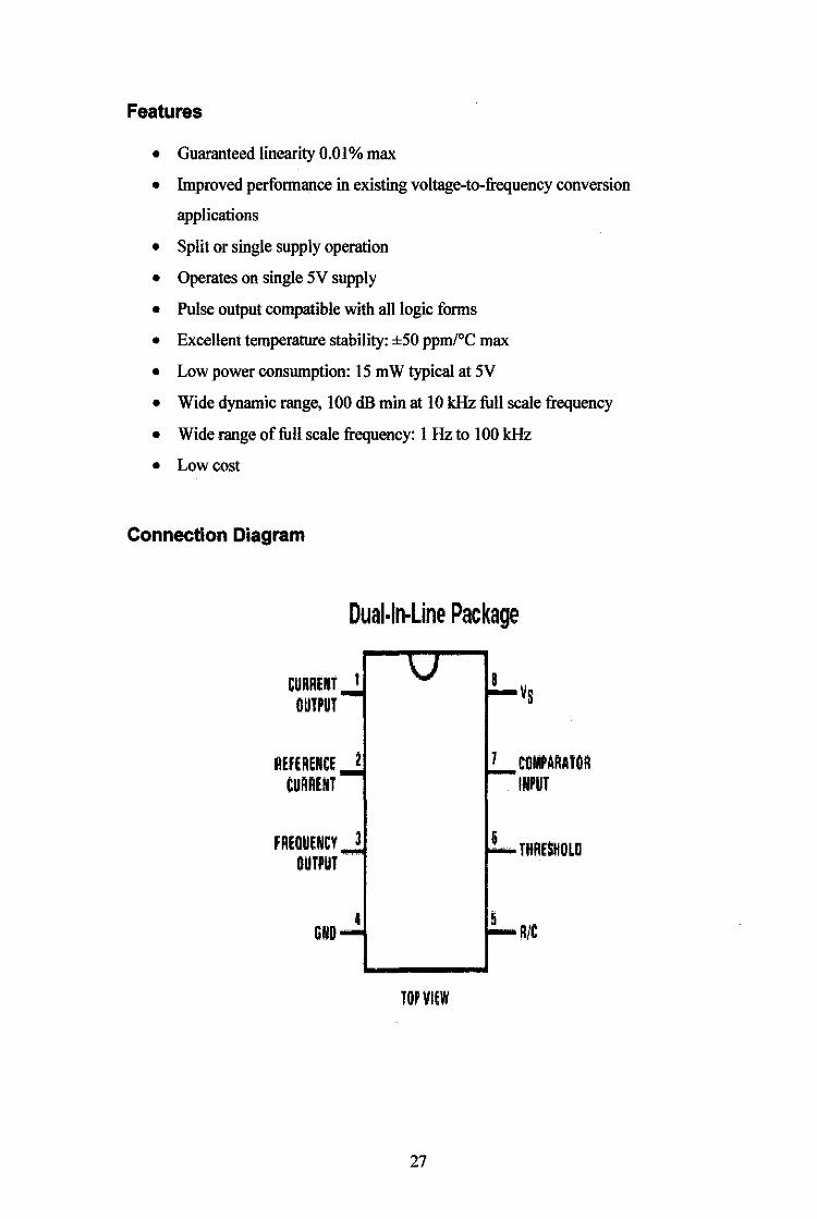
Connection Diagram

Dual-In-Line Package

CURREMT I 8 OUTPUT

REFERENCE CURRENT

FREQUENCY OUTPUT

TOPVI£W

27

COMPARATOR INPUT

RIC

Ordering Information

Device Temperature Range Package

LM231N -25'C 5 TA 5 +S5'C NOSE (DIP)

LM231AN -25'C 5 TA 5 +S5'C NOSE (DIP)

LM331N O'C 5 TA $ +70'C NOSE (DIP)

LM331AN O'C $ T A$ +70'C NOSE (DIP)

Table 1: Ordering Infonnation

Operation Rating

Operating Ambient Temperature

LM231, LM231A -25'C to +85'C

LM331, LM331A o·c to +70'C

Supply Voltage, Vs +4V to +40V

28

Electrical Characteristics All specifications apply in the circun of Figure 4, wnh 4.0V s Vs s 40V, T.=25'C, unless olflerwise specnied.

Parameter Conditions Min Typ Max Units

VFC Non-Linearity (Note 4) 4.5V s Vs s 20V ±0.003 ±0.01 %Full- Scale

T MIN :n, s TMAX ±0.006 ±0.02 %Full- Scale

VFC Non-Linearity in Circuit of Rgure 3 V5 = 15V, I= 10Hz to 11kHz ±0.024 ±0.14 %Full- Scale

Conversion Accuracy Scale Factor (Gain)

LM231. LM231A V1N= -10V, As= 14kl! 0.95 1.00 1.05 kHzf\1

LM331. LM331A 0.90 1.00 1.10 kHzN

Temperature Stability of Gain

LM231/LM331 TM1Ns T,s Tr.w<• 4.5V s Vs!, 20V ±30 ±150 ppmfC

LM231 A/LM331 A ±20 ±50 ppmfC

4.5V s V5 stOV 0.01 0.1 %.N Change of Gain with V5 10VsV5 s40V 0.006 0.06 %f\l

Rated Full-Scale Frequency V1N = -10V 10.0 kHz

Gain Stability vs. Time (1 ooo Hours) TM1N:5:TA$TMAx ±0.02 %Full- Scale

Over Range (Beyond Full-Scale) V1N =-ltV 10 %

Frequency

INPUT COMPARATOR Offset Voltage ±3 ±10 mV

LM231!LM331 Tr-.uNS.TA5Tw.x ±4 ±14 mV

LM231 MM331 A T"1"sT.sTMAX ±3 ±10 mV

Bias Current -80 -300 nA

Offset Current ±8 ±100 nA

Common-Mode Range TMIN$ TA:5 TMAx -o.2 Vcc-2.0 v TIMER

Timer Threshold Voltage, Pin 5 0.63 0.667 0.70 xVs Input Bias Current, Pin 5 Vs = 15V

All Devices OV $ Vp1N 5 $ 9.9V ±10 ±100 nA

LM231/LM331 VPIN 5 = 10V 200 1000 nA

LM231AILM331A VPJN s= 10V 200 500 nA

V SAT PIN 5 (Reset) I= 5 rnA 0.22 0.5 v CURRENT SOURCE (Pin 1)

Output Current

LM231, LM231A A6 =14kll,Vp1N1 =0 126 135 144 ~A

LM331, LM331A 116 136 156 ~A

Change wiTh Voltage ov $ VPIN 1 $ 10V 02 1.0 ~A

Current Source OFF Leakage

29

Electrical Characteristics (Continued) All specn~ations apply in the circuit of Figure 4, wlh 4.0V s V5 $ 40V, T.=25'C, unless otherwise specified.

Parameter I CondHions I Min I Typ I Max I Units CURRENT SOURCE (Pin 1)

LM231, LM231A, LM331, LM331A 0.02 10.0 nA

All Devices T.=TMAX 2.0 50.0 nA

Operating Range of Current (Typical) (10 to 500) ~A

REFERENCE VOLTAGE (Pin 2) LM231, LM231A 1.76 1.89 2.02 Voc LM331, LM331A 1.70 1.89 2.08 Voc

Stability vs. Temperature ±60 ppmf'C

Stability vs. Time, 1000 Hours ±0.1 0' lo

LOGIC OUTPUT (Pin 3) 1=5mA 0.15 0.50 v

VSAT I= 3.2 mA (2 TIL Loads). 0.10 0.40 v

TMINs; TA $; TMAX

OFF Leakage ±0.05 1.0 ~A

SUPPLY CURRENT v, = 5V 2.0 3.0 4.0 mA

LM231, LM231A V5 = 40V 2.5 4.0 6.0 mA

LM331, LM331A Vs=5V 1.5 3.0 6.0 mA

Vs = 40V 2.0 4.0 8.0 mA

Table 2: Electrical Characteristics for LM331

30

Typical Circuit Characteristic

+O.fM ~. +OJIJ ~

fl +0.02 ffi +0.01 > ... "' • ~ ~lUll " ::::; -0.02 ::; z .. a.oJ ....

•

Nonlinearity Error as Precision V -to-F Converter (Figure 4)

I I _j_ I

~EC LIMI.'\ ,,

_...··

' ' "}"'"' '"" SPEC LIMIT

I I I

2 4 ' 8 10 12

FREQUENCY, kHz

Nonlinearity Error vs. Power Supply Voltage

0.025

0,020

~ 0.015 ~

::5 ! 1.010 z a z

uos

O.OOCI

S~CLJ.MIT

~ ,;'

.L'

5 10 15 20 !5 30 35 40

POWER SUPPLY VOL TAG£, VS

VREF vs. Temperature

>

1.930

1.928

1.92i 1.924 1.922

~ 1.1128 :::10 1.918

1.916

1.914

1.112

t,BID -15

...... ..... -...

-25 ... _.15 +1ZS +150

TEMPERATURE. °C

31

+D.Dl

;.t +0.02 ,.· ~ +0.01 1:; > ; 0

" ~ ! -0.01 z 0 z -0.112

-0.03

Nonlinearity Error

D.DOOI O.INJt 0.01 0.1 10 100

"' ,: u ,. w ~ w

"' ~ ... "' 1!: "' ..

FREOUENC'i, kHz

Frequency vs. Temperature

10.06 ,,..,.,..,...,.--,-,--,...,

10.04

+2.0

+1.5

+1.0

+0.5

• -0.5

-1.0

-1.5

-2.0

-55 -25 ... +15 +125

TEMPERATURE, "C

Output Frequency vs, VsuPPLY

5 101fi21253Dl540

VSUPPLY,V

Schematic Diagram

+ •• ;' !l/1 ft.

<l~ ..

* 5•

[;p L5~ '1. fig lJ. ~- ft. •• .,

- 5]

hlb~ u

~~ ., ;;S

'~ •; ~ ;;

f"\~ k"'- •• ., ~ ..

~ j'' ., ~~

k• ~ ~v~>: ~ y-w. I. I "!':."" •

•• ~1, :?.; ' ~ = " I• ~

"*" ".".r .. •.r-•r~· ril.lLLI ·1 .. ~A . -

* • ~ ~lo ~ ~ •l,;s. ••

li(.? §l. lF -~

'•} ~ ~ ~~It .... I'>" • +--«:!! rf ~." l.§ ~

-'I• II ,. ,1·,~ •• ~ §r § I•

~k· !-1.

- ~·-. lJ~~.H • ~~

~K• ~~ 1- ,5,.__ J-_J '..• ·lr=l - I•

;: •

32

APPENDIXC

PRECISION CENTIGRADE TEMPERATURE SENSORS

General Description

The LM35 series are precision integrated-circuit temperature sensors, whose output

voltage is linearly proportional to the Celsius (Centigrade) temperature. The LM35

thus has an advantage over linear temperature sensors calibrated in

o Kelvin, as the user is not required to subtract a large constant voltage from its output

to obtain convenient Centigrade scaling. The LM35 does not require any external

calibration or trimming to provide typical accuracies of ±V4°C at room temperature

and ±3/4°C over a full -55 to +l50°C temperature range. Low cost is assured by

trimming and calibration at the wafer level. The LM35's low output impedance,

linear output, and precise inherent calibration make interfacing to readout or control

circuitry especially easy. It can be used with single power supplies, or with plus and

minus supplies. As it draws only 60 J.lA from its supply, it has very low self-heating,

less than O.l°C in still air. The LM35 is rated to operate over a -55° to +l50°C

temperature range, while the LM35C is rated for a -40° to +ll0°C range (-10° with

improved accuracy). The LM35 series is available packaged in hermetic T0-46

transistor packages, while the

LM35C, LM35CA, and LM35D are also available in the plastic T0-92 transistor

package. The LM35D is also available in an 8-lead surface mount small outline

package and a plastic T0-220 package.

Features

• Calibrated directly in o Celsius (Centigrade)

• Linear+ 10.0 mV/°C scale factor

• 0.5°C accuracy guaranteeable (at +25°C}

• Rated for full -55° to + l50°C range

• Suitable for remote applications

33

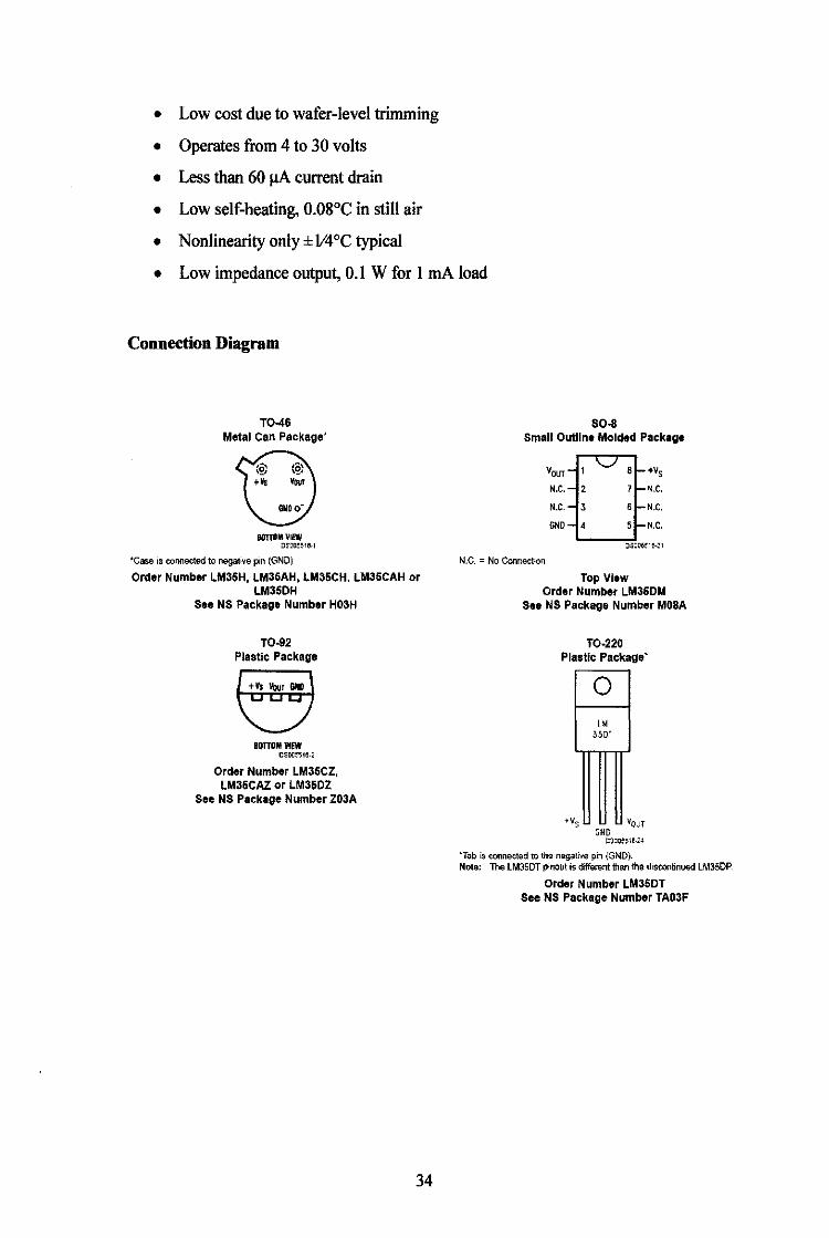
• Low cost due to wafer-level trimming

• Operates from 4 to 30 volts

• Less than 60 !1A current drain

• Low self-heating, 0.08°C in still air

• Nonlinearity only± V4 °C typical

• Low impedance output, 0.1 W for I rnA load

Connection Diagram

T0-46 Metal Can Package'

BOTTOM VIEW D<Dre!-16-1

•case is connected to negative p1n (GND)

Order Number LM35H, LM35AH, LM35CH, LM35CAH or LM35DH

See NS Package Number H03H

T0-92 Plastic Package

Order Number LM35CZ, LM36CAZ or LM36DZ

See NS Package Number Z03A

34

so .a small Outline Molded Package

N.C. = No Connection

YourO' +Vs N.C. 2 7 N.C.

N.C. 3 6 N.C.

GNO 4 5 N.C.

:~:o.:o6~·~,

Top VIew Order Number LM3SDM

See NS Package Number M08A

T0-220 Plastic Package·

0 LM

35DT

H's Vour GHD

DS:Joe:-tC-24

~Tab is connected to the negati·"e pin {GND). Note: The lM35DT pinout is different than the discontinued lM35DP.

Order Number LM35DT See NS Package Number TA03F

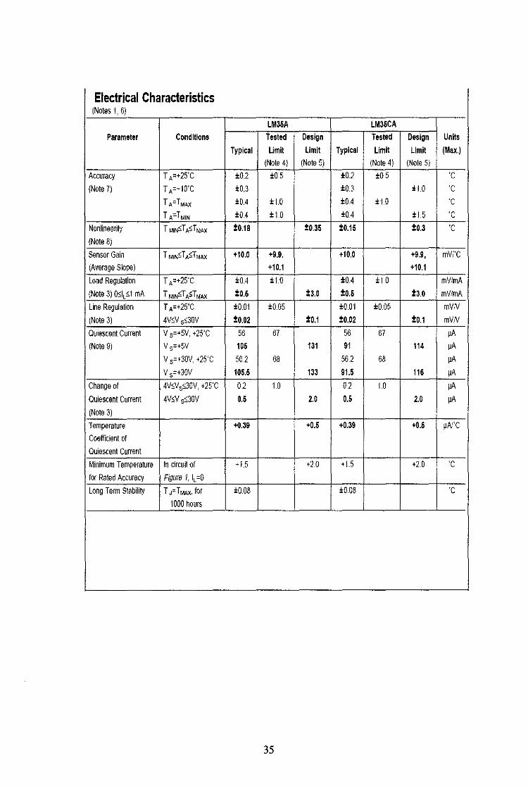
Electrical Characteristics (Notes I, 6)

LM3SA LM3SCA

Parameter Conditions Tested Design Tested Design Units

Typical Limit Limit Typical Limit Limit (Max.)

(Note 4) (Note 5) (Note 4) (Note 5)

Accuracy T •=+25'C ±0.2 ±0.5 ±0.2 ±0.5 'C

{Note 7) T .=-IO'C ±0.3 ±0.3 ±1.0 'C

T .=TMAX ±0.4 ±1.0 ±0.4 HO 'C

T .=T MIN ±0.4 HO ±0.4 ±15 'C

Nonlinearity T MIN:::;T As;T MAX to.ta t0.35 t0.15 to.3 'C

{Note 8)

Sensor Gain T MIN::;TA::;T MAX +10.0 +9.9. +10.0 +9.9, mVI'C

{Average Slope) +10.1 +10.1

Load Regulation T •=+25'C ±0.4 HO ±0.4 HO mVimA

{Note 3) Osl, ,;·t mA T MIN:::;T A$T MAX to.5 t3.0 to.5 t3.0 mVimA

Line Regulation T •=+25'C ±0.01 ±0.05 ±0.01 ±0.05 mVN

{Note 3) 4\15\1 5S30V t0.02 to.1 t0.02 to.1 mVN

Quiescent Current V 5=+5V, +25'C 56 67 56 67 ~A

{Note 9) V 5=+5V 105 131 91 114 ~A

\1 5=+30\1. +25'C 562 68 56.2 68 ~A

\1 5=+30\1 105.5 133 91.5 115 ~A

Change of 4VSV5s30\l, +25'C 0.2 1.0 0.2 1.0 ~A

Quiescent Current 4Vs.V s$30\f 0.5 2.0 0.5 2.0 ~A

{Note 3)

Temperature +0.39 +0.5 +0.39 +0.5 ~AJ'C

Coefficient of

Quiescent Current

Minimum Temperature In circuit of + 1.5 +20 +15 +2.0 ·c for Rated Accuracy Figure I, 1, =0

Long T enm Stability T J= T MAX· for ±0.08 ±0.08 'C

1000 hours

35

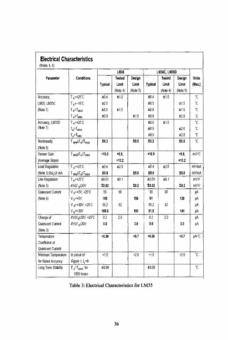
Electrical Characteristics (Notes I. 6)

LM35 LM35C, LM35D Parameter Conditions Tested Design Tested Design Units

Typical Limit Limit Typical Limit Limit (Max.)

(Note 41 (Note 5) (Note 4) (Note 5)

Accuracy, T •=+25'C :1:0.4 :1:1.0 :1:0.4 :1:1.0 'C

LM35, LM35C T .=-IO'C :1:0.5 :1:0.5 :1:15 ·c (Note 7J TA=TMAX :1:0.8 :1:1.5 :1:0.8 :1:15 'C

TA=TMIN :1:0.8 :1:1.5 :1:0.8 :1:2.0 'C

Accuracy, LM35D T •=+25'C :1:0.6 :1:1.5 'C (Note 7) TA=TMAX :1:0.9 :1:20 ·c

TA= TMIN :1:0.[1 :1:2.0 'C

Nonlineanty T MINsT.sT.,AX ±0.3 :!:0.5 :!:0.2 :!:0.5 ·c (Note 8)

Sensor Gain T MIN,TASTMAX +10.0 +9.8, +10.0 +9.8, mVi'C

(Average Slope) +10.2 +10.2

Load Regulation T .=+25'C :1:0.4 :1:2.0 :1:0.4 :1:2.0 mVtmA

(Note 3) OsiL s1 mA T MINsT.sTMAX to.5 :!:6.0 ±0.6 :!:5.0 mVtmA

Line Regulation T •=+25'C :1:001 :1:0.1 :1:0.01 :1:0. I mVN

(Note 3) 4V<J/ 5s30V :!:0.02 :!:0.2 :!:0.02 :!:0.2 mVN

Quiescent Current V 5=+5V, +25'C 56 80 56 80 ~A

(Note 9) V 5=+5V 105 158 91 138 ~A

V 5=+30V, +25'C 56.2 82 56.2 82 ~A

V 5=+30V 105.5 161 91.5 141 ~A

Change of 4VsV5s30V. +25'C 0.2 2.0 0.2 2.0 ~A

Quiescent Current 4V>V 5>30V 0.5 3.0 0.5 3.0 ~A

(Note 3)

Temperature +0.39 +0.7 +0.39 +0.7 ~Ai'C

Coefficient of

Quiescent Current

Minimum Temperature In circuit of +1.5 +2.0 +1.5 +2.0 ·c for Rated Accuracy Figure I. IL =0

Long Term Stability T J= T1.1AX• for :1:008 :1:0.08 ·c ·1000 hours

Table 3: Electrical Characteristics for LM35

36

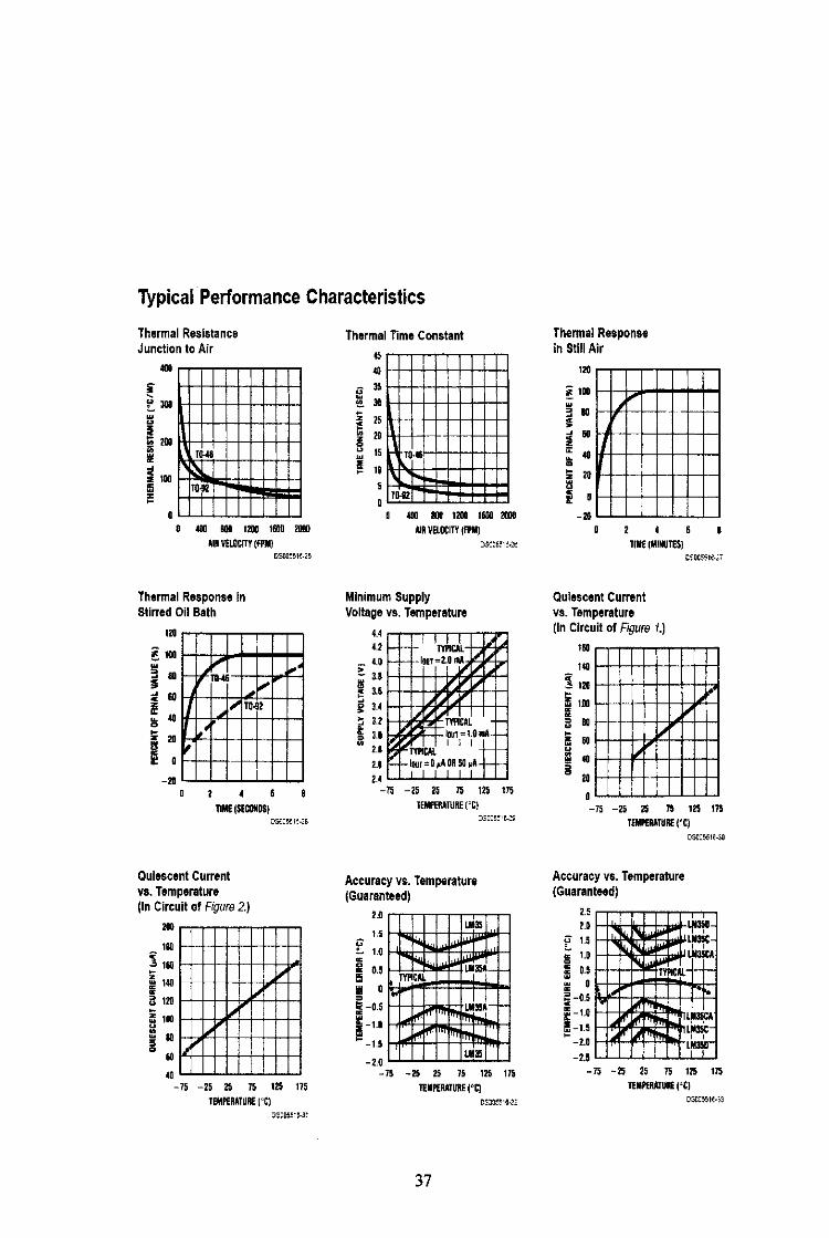
Typical Performance Characteristics

Thermal Resistance Junction to Air

010

TIH&

~ 10-92

0 J 0 4111 800 1200 1600 2000

AIR VELOCITY (FPM)

Thermal Response In Stirred Oil Bath

uo ! 1(10 w 3 80 !I ~ 80 c !!

<0 ~ 0 ~

~· I-' ·" T0-92

~·

z ,. !I ~· ·f-f-E

II! 0 _,.

' 2 • 6 nME (SEI:GOOS)

Quiescent Current vs. Temperature (In Circuit of Figure 2.)

200

181

l181

ffi 140 i 0: 120

11= co

.

"" ~

-75 -25 25 75 125 175 TEMPERATURf i"Ci

Thermal Time Constant

15 <0

ll: 35

e 30

I I I

~ z 15 ~ 10 ~ 15 w TO·U ~ 11

5

0 Tll.JZ

' ... llJO 1208 1608 2000 Al1l VElOCITY (IPM)

Minimum Supply Voltage vs. Temperature

4.4 4.1

-. 4.0 > ii3.1 ~ 3.6

~ u ~ a.z ~ 3.0

2.8

1.8 2.4

f- .I 1TY~C~ -lour=Z.O .....

"" .NL;'TY1'1CAL

~tt)l,mrr=1:t ~ ll I 111'1CAL j-loor

1=o,-•

10R ~ ~·

-75 -25 25 15 125 175 TEMPBIATURE {°C)

Accuracy vs. Temperature (Guaranteed)

r E

2.0

1.5

1.0

a 0.5

Ill 0 ~ -0.5

1-10 -1.5

-2.0

LM35

""'" Ll3~-

~,.J_

LM35

-75 -25 25 75 125 17S TEMPERATURE ('C)

O~:J!);~I~Z

37

ThennaiResponss in Still Air

110 rT--r-r-rT"r'r-1

i 1110 H-t:;;ol--1-+++-l 3 IKIH~HH-!1 i 60

l!; " lf1H-+-+-+-+-t-+ ~ 20 HHHHH-t-t-l

~ o HH-+-+-+-t-t-1 -111 L..l.-L.~.l-l-J.-.L._J

0 • 6 nME !MINUTES)

Quiescent Current vs. Temperature (In Circuit of Figure l.)

160

1<4

'j;11G ~

m , .. E

B BO

i5 " I 40 10

0

I ! .

I

~

"" I

8

...

-75 -25 25 15 125 175 TEMPERATURE (•CJ

DSC:5iile->O

Accuracy vs. Temperature (Guaranteed)

2.S 1.1

~1.5 !! 1.1 ffi 0.5 ~ 0

i=~:: !-1.5 ,_ -Z.O

-2.5

~~ TYIICAl

~

~

LMIID ' ' ~~

UI3$CA

LM3$CA LM!ic

i ' LM~o-

-75 -25 25 15 125 115 TEMPERATURE ('C)

DSC~~51e-;o

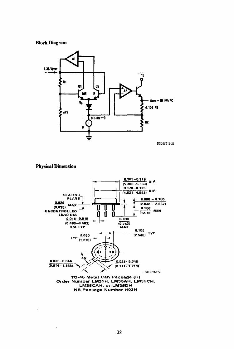
Block Diagram

1.38Vmr -- t----i---1--,

R1 01 02

Vour=10 mYJ•c

0.125 R2 nR1

RZ

--

Physical Dimension

0.100 ~-+-------(2.540) TYP

T0-46 Metal Can Package (H) Order Number LM35H, LM35AH, LM35CH,

LM35CAH, or LM35DH NS Package Number H03H

38

DSJOE515-2~·

APPENDIXD

QUAD 2 INPUT SCHMITT NAND GATE

Features

• High speed

• Tpd = II ns (typ.) At vee= 5 v lowpower dissipation

• Icc= IDa (max.) At ta = 25 De output drive capability

• I 0 lsttlloads high noise immunity

• Vh (typ.) = 0.9 vat vee= 5 v symmetrical output impedance

• DiohQ= iol = 4 rna (min.) Balancedpropagation delays

• Tplh = tphl wide operating voltage range

• Vee (opr) = 2 v to 6 v pin and function compatible with 54/741sl32

Description

The M54/74HCI32 is a high speed CMOSQUAD2-INPUT SCHMITT NAND GATE

fabricated in silicon gate C2MOS technology. It has the same high speed performance

ofLSTTL combined with true CMOS low power consumption. Pin configuration and

function are identical to those of the M54/74HCOO. The hysterisis characteristics

(around 20 % VCC) of all inputs allow slowly changing input signals to be

transformed into sharply defined jitter-free output signals. All inputs are equipped

with protection circuits against static discharge and transient excess voltage.

39

PIN CONNECTIONS (top view)

NC• No ln1ernal connectbn

... ta

,., ... ... ......

IY

He ... ftC

••

ABSOLUTE MAXIMUM RATINGS

svmbol Parameter Vee Suoolv Vottaae v, DC Input Voltage

r--Yo DC Output Voltage ·----·-----loK DC lnout Diode Current

loK DC Output Diode Current

lc DC Output Source Sink current Per Output Pin

Icc Of IGND DC Vee or Ground Current Po Power Dlssloatlon

~· Storage Tem~erature

T, Lead Temoerature 110 secl

. .. "" .. NC

IB

··-Value

-0.5 to +7

-0.5 to Vee + 0.5

-···--·0.5 to Vee ~---±20 ±20

·~·------

±25 +50 --··

BOO /"I

-65 to +150 -300

Unit v v

_ _y__ mA mA mA mA mw 'C 'C

Absolute Max1mum R3tingsare thoS&values be~nd whlchdarm;;~e -othedEJYICe mcl.fo<:cii. Fur:ctlonal opg-aJon und:lr 1hese condttonlsnotlmplied (~i 500 n'./o,': .a. 65 <t derate to 300 nl.PJ by 10m'.JI.•fc: 65 OC :o 85 •c

Table 4: Absolute Maximum Rating for NAND Gate

40