Designing successful product demonstration campaigns in australia

Designing a High Speed
Network for Australia
Beyond Zero Emissions
Kerrin Beovich, James DeCelle, Shaun Marshall, & Wilfredo
Ramos
2/29/2012

i
Abstract
Australia’s rail network does not provide enough for its passengers. It lacks a high speed
network and is disconnected: providing travel radial with respect to Melbourne and Sydney, but no
crossing lines. The team utilized the experience of international rails to examine Australia’s
transportation needs, based upon coverage, convenience, and cost. Drawing upon rail networks from
other countries, the team proposed a new rail network for Australia that was accessible to 80% of the
population. The final proposal was based upon coverage, convenience and cost, and offers travelers
within Australia with a more connected rail network and access to high speed lines.

ii
Acknowledgements
We would like to extend our thanks to the following individuals and organizations for their
assistance in the completion of our project:
Beyond Zero Emissions and volunteers for sponsoring our project, providing us with a great
work environment, always greeting us with a warm welcome, and providing helpful feedback on
our project.
Patrick Hearps, our project liaison, for aiding us with his extensive idea, knowledge, and
resources.
Matthew Wright, executive director of BZE, for his constant support and warm personality.
Courtenay Wheeler for taking the time to meet with us and help us with the GIS software.
Adrian Whitehead for his friendly greetings and hospitality.
Professor Stanley Selkow, our project advisor, for providing guidance and critical feedback
throughout our entire project.
Mrs. Deb Selkow for taking the time to meet with the group and provide helpful edits.
Holly Ault, our Project Center Director, for all her work in preparing us to travel to Melbourne
and providing us with the opportunity to take part in our project.
Andrea Bunting for providing helpful information on the city of Melbourne itself and her
contributions to the onsite events.

iii
Authorship Page
Kerrin Beovich – Contributed to the Introduction and Background Chapters. She wrote Most of the
“Global Warming” and “Transportation” sections of the Background chapter. She wrote “The Gap”
sections and parts of the “Rail Network Coverage” and “Convenience” sections as well. She wrote the
“Research Methods”, “Why the Analysis of US Rail” and “Analyzing the Collected Data” sections. She
also researched the information regarding France and the US and wrote their corresponding sections in
the Findings chapter, as well as the “International Rail Networks Information”, “Cost per Kilometer of
Rail”, “Possible Upgrades/Proposals”, “Limitations of Research”, and “Information Acquisition” sections
of the Findings chapter. She wrote/compiled Appendix A and formatted most figures and tables
throughout the report. She also contributed to the general editing and revising of the report, the
gathering and formatting of the Appendices, and she managed the format and structure of our paper.
James DeCelle – Wrote most of the executive summary and the introduction chapters. He contributed
to the research of the “Transportation” and “Building a Successful Rail Network” sections of the
Background chapter and wrote the “Global Warming” section, “Buses” section, “Trains” section, all of
the “Australian Rail” sections, much of the “Rail Network Coverage” and “Convenience” sections, and
the “What Is Missing” section. He also wrote all sections, excluding the Why the Analysis of US Rail
section, in the Research Methods. He researched the information regarding Great Britain, Italy, and
Japan, and wrote their sections in the Findings Chapter as well. He wrote the conclusions and
recommendations chapter and contributed to the general editing and revising of our report.
Shaun Marshall – Contributed to the Background and Findings chapters, researching all information on
Germany and Switzerland. He also wrote the “Cost”, “Frequency” and “Travel Times” sections and parts
of the “Accessibility” section in the Background chapter. He also contributed to the Findings chapter
and wrote the “Station Location and Population” section. He also wrote Appendices B-G. He
contributed to much of the general editing and revising of our report.
Wilfredo Ramos – Contributed to Background and Findings chapters. He gathered research on Spain
and Australia, and wrote their corresponding sections in the Findings chapter. He generated all
population density, elevation, and rail network maps using both Photoshop and GIS software. His main
focus was the revising of our paper.

iv
Executive Summary Introduction and Background
Global Warming is a complex yet serious societal issue resulting in rising sea levels; sea-surface
temperatures; and humidity, and the disappearance of glaciers (IPCC, 2007). Global Warming occurs as
excessive amounts of greenhouse gases, for example carbon emissions1, are released into the
atmosphere (Carbon Dioxide Information Analysis Center (CDIAC)). Once released, carbon emissions are
absorbed by sinks, such as plants and oceans, which process the carbon dioxide until oxygen is released;
however, the sinks are not able to support the current rate at which carbon dioxide is being emitted
(EPA). Steps must be taken in order to decrease the amount of carbon dioxide released into the
atmosphere (Agency, 2006).
In the year 2000, transportation was the third leading contributor to greenhouse gases world-
wide. Road transportation was the second leading contributor among all sub-sectors2, where public
transportation was one of the least carbon emissive among all sub-sectors (World Resources Institute,
2008). By 2007, the transport sector had become the second leading contributor of carbon emissions
(Internation Transport Forum, 2010). Studies show that trains emit up to 75% less carbon emissions per
passenger kilometer3 than automobiles; therefore, creating a shift from road to rail transportation has
the potential to reduce world-wide carbon emissions from road transportation by as great as 75%
(Ludewig & Aliadiere, Rail Transport and Environment: Facts and Figures, 2008).
In order to create the shift from road to rail, rail transportation needs to become more
appealing to passengers (UNEP). A common method doing so is to create a high speed network that
enables passengers to reach their destinations at speeds of 250km/h or faster, which countries such as
France, Italy, Japan, and Spain have already begun to utilize (See Appendix H). London and the United
States are currently in the early stages of constructing new high speed rail networks through planned
proposals, the High Speed 2 and America 2050, respectively (ibid). In addition to constructing a high
speed network, providing the desired road to rail shift can be achieved by creating a rail network that
covers (rail network coverage)4 enough of its targeted population and is adequately accessible5. Studies
in England have concluded that one of the main reasons automobile users do not use public
transportation, such as trains, is that the trains are not accessible to passengers (Kamba, O.K. Rahmat, &
Ismail, 2007). The same study also concluded that the lack of public transit use is due to convenience6
1 Carbon, an element, is not a greenhouse gas; however, carbon dioxide, which is a greenhouse gas, is commonly
shortened to carbon for ease of reference (Torchbox). 2 Each sector of carbon emission sources is broken into multiple sub-sectors, such as air travel, rail transport, road
transport, etc. Of all these sub-sectors, road transportation is the second leading contributor 3 Passenger-kilometer refers to the one kilometer traveled by a passenger (someone who is traveling by the
method of transportation reference [car, train, etc.]) 4 The rail network’s accessibility to its passengers and its ability to provide the options of high speed (250+ km/h),
fast (200-250 km/h), or basic (<200 km/h) trains within the city of the station or an adjacent city 5 The rail network’s ability to provide its passengers with access points and destinations that fulfill their needs
6 The rail network’s ability to provide services frequently throughout a daily operational period that is able to fulfill
passengers’ needs

v
(ibid). In order to entice people into consistently using the trains, rail networks are being operated on
frequent intervals, such as offering train services 2-4 times per hour (See Appendix H.1.3).
While rail network coverage and convenience are factors that can help or hinder a shift from
road to rail, there exists a limitation: cost7. Providing coverage to 100% of a region’s population and
operating trains that run every 5 minutes would certainly enable a massive (if not complete) shift from
road to rail; however, it is unrealistic due to the cost. Depending on the distance covered and the type
of terrain involved, high Speed rail lines within a rail network can cost upwards of $100 billion AUD; the
cost of the high speed line between Melbourne and Brisbane (a distance of 1600 km) is estimated
between $61-108 billion AUD (Rood, 2011). Furthermore, the price of extending and/or upgrading a rail
network is dependent on the type of work done on the rail lines within the network. Upgrading an
existing rail line is cheaper than building a completely new one, and rail line costs vary depending on the
terrain (tunneling, bridging, etc.) (See Appendix H). Funding is a limited resource and plays an influential
role in all major decisions; thus, understanding the cost of its various components of it enables the
construction of a rail network that will appeal to its target population both effectually and economically.
Australia is in the process of extending/upgrading its rail network. The country’s rail network
lacks any high speed rail lines and is very disconnected (See Appendix C). Australia’s flawed rail network
hinders its ability to shift its passengers from road to rail, even though, in recent years, there has been a
growing desire for public rail use. Studies have been conducted throughout Australia; areas such as
Melbourne are showing an increased desire to use public transportation; and additionally, there has
been an increase in rail usage (Low, 2008). Unfortunately, the current rail network does not have the
capacity to support this growing desire; however, the government recognizes this and is researching
high speed lines and upgrades to the current rail network (ibid).
High speed lines have been, and are being researched, to connect the major cities8 of Australia
(Rood, 2011). The major cities are not only home to over 50% of the population of Australia, but are
popular tourist attractions (both domestically and internationally), thus, justifiable of a high speed rail
(Tourism Research Australia, 2011). A rail network that can compete with automobiles, and airplanes, in
terms of travel times and frequency9 between the major and popular cities can give the public an
alternative option to driving their automobiles. Upgrades to the current rail network, such as new
crossing routes and a new line connecting Melbourne and Mildura, are also being researched (AECOM,
2010). The lack of connectivity10 and the need for more rail lines are recognized and a new proposal is in
the making (ibid).
Beyond Zero Emissions (BZE), a non-profit organization, has begun researching the current state
of Australia’s rail network and creating its own rail network proposal, both upgrading current rail lines
and creating new rail lines (such as a high speed line) (Wright & Hearps, 2010). The organization
7 Cost of building the rail lines which includes the planning and land costs, infrastructure building costs, and super
structure costs 8 Perth, Adelaide, Melbourne, Sydney, and Brisbane (the 5 most populated cities in Australia)
9 The interval at which a train departs from a train station
10 The average number of connections a station provides (See Appendix C for further detail)

vi
collected data on Australia; however designing a rail network should consider the rail networks of other
countries, especially ones that are considered to be successful, or ones that are currently going through
upgrades and installations similar to those necessary for Australia’s rail network. If the other countries
with successful rail networks can be analyzed to determine why they are successful, the knowledge
gained from the analysis and studies can help with the construction of our rail network proposal. Also,
understanding why other countries’ rail networks fail, or do not perform as well as others, can be of use.
Research Methods
We acquired information on international rail networks regarding coverage11, convenience, and cost.
After analyzing the data found on other countries, we constructed a rail network proposal for Australia.
In order to achieve this goal, the completion of three objectives was necessary:
Gathering information on the entire12 rail networks of France, Germany, Great Britain, Italy,
Japan, Spain, Switzerland, and US
Analyzing these countries’ rail networks using the criteria of rail network coverage, convenience,
and cost
Proposing a feasible rail network that covers 80% of Australia’s population
The selection of countries for this study was carefully considered. European countries were
chosen because they contain some of the most prominent, widely utilized rail networks in the world.
Europe possesses a high amount of high speed track, and many countries either have plans or are
already in the process of expanding their current network. For example, Great Britain has a High Speed
2 proposal that has been approved by the government (Department for Transport, 2012). Similarly, the
United States is creating a high speed rail proposal (America 2050), which the country currently lacks
(High Speed Rail in America). The proposals in Great Britain and the US proved useful because they are
similar to the types of upgrades and installations that Australia desires. Japan’s rail network was chosen
for study because it is the pinnacle of high speed rail. Many countries around the world base their high
speed train technology off of Japan’s (Mong, 2010). The country is also home to the most high speed
track, as of 2008 (Milmo, 2009). Once the desired countries for this study were selected, we began
collecting our data.
An Excel spreadsheet was constructed as a template in order to organize the information on
each country’s rail network. The spreadsheets were organized into the three main categories: coverage,
convenience, and cost. Each category was comprised of specific information.
Coverage information contained station location with respect to the population of each country
and the type of rails13 along each rail line within the rail networks. When gathering and organizing the
11
Italicized words can be found in the glossary (See Appendix A) 12
Including all high speed, fast speed and basic rails throughout the country

vii
station population and population data, each city/town with a train station was found and placed into
the excel spreadsheet. The sum of the people residing in a city/town with a train station was divided by
the total population of the given country. This statistic was called “Station Population Ratio (SPR).”
Adjacent cities/towns were not included in this SPR because we did not have access to such
sophisticated software or sufficient data, to allow for it. We countered this lack of data by
superimposing maps of each country’s rail networks over maps of the population densities. These maps
allowed us to study the location of train stations in relation to the population of each country. In
addition to SPR, the group determined the type of train that each train station utilizes. These data was
mainly used to determine where the high speed trains stop. These data allowed the group to compare
the accessibility and coverage of the various rail networks.
Convenience information contained data regarding the service frequency offered along the
different rail lines and the travel times between popular destinations. The service frequencies and the
travel times evaluated the ability of the rail networks to be convenient for its passengers, which was a
major influence on whether people use public transportation (Kamba, O.K. Rahmat, & Ismail, 2007).
The cost spreadsheets were comprised of different situational costs and total length of various
rail line/network projects all over the world. A normalized14 cost per kilometer of track was sought for
each country. This information was important in estimating the cost of the rail lines within our
Australian rail network proposal. The cost of other projects around the world, along with the cost of
prior Australian projects, was used by a member of BZE to construct an estimate of cost per kilometer of
track for different terrains (Urban, Tunneling, Mountainous, Elevated Track, Undulating, and Flat
Farmland) (See Appendix H).
Important Findings
Our data showed that:
Coverage
o Majority of tracks (for international rails) lie in highly populated areas (See Appendix H)
o International rails have a higher connectivity than Australia (See Appendix C)
Australian average number of direct connections: 1.5
International networks range from 2.3-2.6
o A high speed line should not have many stops
Convenience
o The more successful rails run more frequently (See Appendix H)
Cost
o Cost ultimately comes down to what terrain the rail must cross/cut through (See
Appendix G)
13
Refers to the maximum speed a train is able to run along a give rail line. These are classified into three main categories: High Speed (250+ km/h), Fast Speed (200+ km/h), and Basic Speed (<200 km/h) 14
The cost of building a rail with no obstacles or terrain difficulties

viii
The SPR for the international rails ranges from 19% (US) to 66% (Great Britain). Some countries
had a low SPR because the train stations were located just outside of major cities (See Appendix H). A
majority was found in larger populated cities/town, but for every country, we found stations (high, fast
and basic) in very small cities/towns. These small cities/towns were usually major tourist attractions
(i.e. Ueno, Japan and Limone, Italy).
As for frequency, each rail differed depending on the time of day and the day of the week. Rail
networks run trains at higher frequencies during rush hour15. Japan had one of the best train schedules
due to its use of all three types of trains on the same track during the same hour; many of the rails in
Japan run the high speed train 4 times an hour throughout the day, with 1 or 2 more trains operating
during rush hour. In most other countries, it was normal to see the high speed train run on a track once
or twice an hour (See Appendix H.1.3).
The cost16 also varied country to country, but more notably was the cost for building a new rail,
upgrading a current rail, and tunneling. Denmark began building a metro line which consisted of all
underground routes and was estimated at $247.5 million/km. Upgrades in France, England, Switzerland
and Spain cost about $24 million/km, $44 million/km, $83 million/km, and $1.6 million/km, respectively.
To build new high speed rails in France, Spain and Italy, the normalized cost for both France and Spain is
approximately $11.5 million.km, while in Italy the normalized cost is about $28.8 million/km (See
Appendix H.1.2).
While the information collected on each country proved useful, the rising question was whether
the countries studied were comparable to Australia (See Appendix H). Countries such as France,
Germany, Great Britain, Spain, and Switzerland are comparable to Australia because these countries are
densely populated in and around their major cities, just as Australia. The major difference between
these countries and Australia is that Australia is at least 12 times larger (ibid). The US is similar to
Australia because a large amount of people are concentrated along the east and west coast and there is
a large amount of land in the middle of the country with lower populated areas. The similarities with
Italy and Japan, however, need to be more closely looked at. Italy is more densely populated than
Australia, but like Australia, it is very populated in and around the 5 or so major cities (Rome, Milan,
Venice, Naples, etc.) and a big drop off in population density the further away one is from the major
cities. Japan needs a much closer look; the entire country is densely populated, with no real
unpopulated areas. What makes Japan comparable is its similarity to the southeastern and eastern
coast of Australia. Much of Australia’s population is located along this strip (between Melbourne and
Brisbane) and is comparable to Japan. The rail networks of Japan can play an important role in the high
speed proposal located along the Melbourne-Brisbane corridor. Although the similarities can be
inconspicuous, the countries chosen all have their similarities to Australia that allowed for helpful
information while constructing our proposal of Australia’s rail network (See Appendix H).
15
06:00-10:00; 15:00-18:00 16
Necessary adjustments were made to normalize the different costs, inflation and currency exchange rates were used for normalization (Coinnews Media Group LLC) (OANDA, 2012)
ix
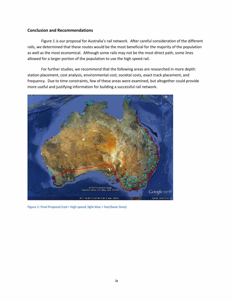
Conclusion and Recommendations
Figure 1 is our proposal for Australia’s rail network. After careful consideration of the different
rails, we determined that these routes would be the most beneficial for the majority of the population
as well as the most economical. Although some rails may not be the most direct path, some lines
allowed for a larger portion of the population to use the high speed rail.
For further studies, we recommend that the following areas are researched in more depth:
station placement, cost analysis, environmental cost, societal costs, exact track placement, and
frequency. Due to time constraints, few of these areas were examined, but altogether could provide
more useful and justifying information for building a successful rail network.
Figure 1: Final Proposal (red = high speed, light blue = fast/basic lines)

x
Table of Contents
Abstract .......................................................................................................................................................... i
Acknowledgements ....................................................................................................................................... ii
Authorship Page ........................................................................................................................................... iii
Executive Summary ...................................................................................................................................... iv
Table of Contents ......................................................................................................................................... x
List of Figures .............................................................................................................................................. xiv
List of Tables ............................................................................................................................................... xv
I. Introduction ....................................................................................................................................... 1
II. Background ........................................................................................................................................ 2
1. Global Warming ................................................................................................................................ 2
1.1. What Are Carbon Emissions ...................................................................................................... 2
1.2. What will happen if the level of carbon emissions is not reduced? ......................................... 2
2. Transportation .................................................................................................................................. 2
2.1. Automobiles .............................................................................................................................. 3
2.1.1. Gas-Consuming Automobiles ............................................................................................ 3
2.1.2. Hybrid and Electric Automobiles....................................................................................... 3
2.2. Carbon Free Methods of Transportation .................................................................................. 4
2.3. Public Transportation ................................................................................................................ 4
2.3.1. Buses ................................................................................................................................. 4
2.3.2. Trains ................................................................................................................................. 5
3. Australian Rail ................................................................................................................................... 5
3.1. Current State ............................................................................................................................. 5
3.2. Desired Improvements.............................................................................................................. 6
4. Building a Successful Rail Network ................................................................................................... 7
4.1. Cost ........................................................................................................................................... 7
4.1.1. Measure against Benefits.................................................................................................. 7
4.1.2. External Costs .................................................................................................................... 7
4.2. Rail Network Coverage .............................................................................................................. 8
4.2.1. Accessibility ....................................................................................................................... 8
4.2.2. Type of Rail ........................................................................................................................ 8

xi
4.3. Convenience .............................................................................................................................. 8
4.3.1. Frequency .......................................................................................................................... 9
4.3.2. Travel Times ...................................................................................................................... 9
5. The Gap ............................................................................................................................................. 9
5.1. What Is Known .......................................................................................................................... 9
5.2. What Is Missing ......................................................................................................................... 9
III. Research Methods ....................................................................................................................... 11
1. Examination of International Rail Networks ....................................................................................... 11
1.1. Why the Analysis of European Rail Networks .............................................................................. 11
1.2. Why the Analysis of US Rail.......................................................................................................... 12
1.3. Why the Analysis of Japanese Rail ............................................................................................... 12
1.4. Gathering the Information ........................................................................................................... 12
1.4.1. Coverage ............................................................................................................................... 12
1.4.2. Infrastructure of Rails ........................................................................................................... 13
1.4.3. Convenience of Rails ............................................................................................................. 13
1.4.4. Cost of Rails ........................................................................................................................... 13
1.4.5. Future Expansion of Rails ...................................................................................................... 13
2. Analyzing the Collected Data .............................................................................................................. 14
2.1. The Data ....................................................................................................................................... 14
2.2. The Data Analysis ......................................................................................................................... 14
3. The Proposal ....................................................................................................................................... 14
3.1. 80% Coverage ............................................................................................................................... 14
3.2 Different Rail Lines ........................................................................................................................ 15
4. Summary ............................................................................................................................................. 15
IV. Findings/Results ......................................................................................................................... 16
1. International Rail Networks Information ............................................................................................ 16
1.1. Station Location and Population ............................................................................................. 16
1.1.1. Overview ......................................................................................................................... 16
1.1.2. France .............................................................................................................................. 17
1.1.3. Germany .......................................................................................................................... 18
1.1.4. Great Britain .................................................................................................................... 18
1.1.5. Italy .................................................................................................................................. 18

xii
1.1.6. Japan ............................................................................................................................... 19
1.1.7. Spain ................................................................................................................................ 19
1.1.8. Switzerland ...................................................................................................................... 19
1.1.9. US .................................................................................................................................... 19
1.2. Frequency and Time ................................................................................................................ 20
1.2.1. France .............................................................................................................................. 20
1.2.2. Germany .......................................................................................................................... 20
1.2.3. Great Britain .................................................................................................................... 20
1.2.4. Italy .................................................................................................................................. 21
1.2.5. Japan ............................................................................................................................... 21
1.2.6. Spain ................................................................................................................................ 21
1.2.7. Switzerland ...................................................................................................................... 22
1.2.8. US .................................................................................................................................... 22
1.3. Cost per Kilometer of Rail ....................................................................................................... 22
1.3.1. France .............................................................................................................................. 22
1.3.2. Germany .......................................................................................................................... 22
1.3.3. Spain ................................................................................................................................ 23
1.3.4. Switzerland ...................................................................................................................... 23
2. Australia vs. international rails ....................................................................................................... 23
2.1. France ...................................................................................................................................... 23
2.2. Germany .................................................................................................................................. 24
2.3. Great Britain ............................................................................................................................ 24
2.4. Italy .......................................................................................................................................... 24
2.5. Japan ....................................................................................................................................... 24
2.6. Spain ........................................................................................................................................ 24
2.7. Switzerland .............................................................................................................................. 25
2.8. US ............................................................................................................................................ 25
3. Possible Upgrades/proposals .......................................................................................................... 25
4. Limitations of Research ................................................................................................................... 26
4.1. Information Acquisition .......................................................................................................... 26
4.2. Biases ...................................................................................................................................... 27
V. Conclusions and Recommendations ............................................................................................ 28

xiii
Bibliography ................................................................................................................................................ 32
Appendix A: Glossary .................................................................................................................................. 38
Appendix B: Cost-Benefit Analysis .............................................................................................................. 39
Appendix C: Connectivity ............................................................................................................................ 41
Appendix D: Population Distribution Weighting......................................................................................... 45
Appendix E: Locomotive Dynamics ............................................................................................................. 49
Appendix F: Travel Time Assessment.......................................................................................................... 53
Appendix G: Optimization of Parameters ................................................................................................... 54
Appendix H: Findings .................................................................................................................................. 59

xiv
List of Figures
Figure 1: Final Proposal (red = high speed, light blue = fast/basic lines) ..................................................... ix
Figure 2 Current Rail Map of Australia (Nye, 2011) ...................................................................................... 6
Figure 3 Australia’s Population (Google Earth) ............................................................................................. 6
Figure 4 High Speed Rail Proposal (Google Earth) ...................................................................................... 26
Figure 5 Australian Rail Network Proposal ................................................................................................. 28
Figure 6 Adelaide to Melbourne Corridor ................................................................................................... 29
Figure 7 Melbourne – Sydney Corridor ....................................................................................................... 29
Figure 8 Rail Network Connectivity ............................................................................................................. 30
Figure 9 Initial Rail Network Connectivity ................................................................................................... 42
Figure 10 Population Distribution by Connectivity ..................................................................................... 43
Figure 11 Cumulative Population by Cumulative Cities .............................................................................. 45
Figure 12 Population Distribution by Percentiles - Australia ...................................................................... 46
Figure 13 Population Distribution by Percentiles – Great Britain ............................................................... 47
Figure 14 Approximate Acceleration of Locomotive .................................................................................. 50
Figure 15 Approximate Deceleration of Locomotive .................................................................................. 51
Figure 16 Depiction of All Possibile Alternative High Speed Rail Lines ....................................................... 55
Figure 17 Elevation Profile (left) and Population Density (right) for France with Rail Map ....................... 59
Figure 18 Elevation Profile (left) and Population Density (right) for Germany with Rail Map ................... 70
Figure 19 Elevation Profile (left) and Population Density (right) for Great Britain with Rail Map ............. 76
Figure 20 Elevation Profile (left) and Population Density (right) for Italy with Rail Map ......................... 117
Figure 21 Elevation Profile (left) and Population Density (right) for Japan with Rail Map ....................... 119
Figure 22 Elevation Profile (left) and Population Density (right) for Spain with Rail Map ....................... 123
Figure 23 Elevation Profile (left) and Population Density (right) for Switzerland with Rail Map ............. 130
Figure 24 Elevation Profile (left) and Population Density (right) for the US with Rail Map ..................... 139
Figure 25 Average Unit Cost for international rails .................................................................................. 151
Figure 26 Travel Times for France TGV ..................................................................................................... 151
Figure 27 Elevation Profile (left) and Population Density (right) for Australia with Rail Map .................. 172
Figure 28 High Speed Rail Options from Adelaide to Melbourne ............................................................. 173
Figure 29 High Speed Rail Option from Perth to Adelaide ....................................................................... 173
Figure 30 High Speed Rail Option from Brisbane to Cairns ...................................................................... 174
Figure 31 High Speed Rail Options from Melbourne to Sydney ............................................................... 174
Figure 32 High Speed Rail Options from Sydney to Brisbane ................................................................... 175

xv
List of Tables
Table 1 Coverage Summary Table for International Rails ........................................................................... 17
Table 2 Comparison of Optimized High Speed Lines .................................................................................. 56
Table 3 Population of Cities/Towns in France with Stations ...................................................................... 59
Table 4 Summary of Coverage for France ................................................................................................... 70
Table 5 Population of Cities/Towns in Germany with Stations .................................................................. 70
Table 6 Summary of Coverage for Germany ............................................................................................... 76
Table 7 Population of Cities/Towns in Great Britain with Stations ............................................................ 77
Table 8 Summary of Coverage for Great Britain ....................................................................................... 117
Table 9 Population of Cities/Towns in Italy with Stations ........................................................................ 117
Table 10 Summary of Coverage for Italy ................................................................................................... 119
Table 11 Population of Cities/Towns in Japan with Stations .................................................................... 119
Table 12 Summary of Coverage for Japan ................................................................................................ 123
Table 13 Population of Cities/Towns in Spain with Stations .................................................................... 123
Table 14 Summary of Coverage for Spain ................................................................................................. 130
Table 15 Population of Cities/Towns in Switzerland with Stations .......................................................... 130
Table 16 Summary of Coverage for Switzerland ....................................................................................... 138
Table 17 Population of Cities/Towns in the US with Amtrak Stations ...................................................... 139
Table 18 Summary of Coverage for the US ............................................................................................... 147
Table 19 Cost of Building Rails/km from International Rails .................................................................... 147
Table 20 Travel Times and Frequencies for German Rails ........................................................................ 151
Table 21 Travel Time and Frequency of Rail in Great Britain ................................................................... 154
Table 22 Travel Times and Frequencies for Italian Rail ............................................................................ 156
Table 23 Travel Times and Frequency of Japanese Rail ............................................................................ 158
Table 24 Travel Times and Frequency of Spanish Rails ............................................................................ 163
Table 25 Travel Times and Frequency of Swiss Rails ................................................................................ 166
Table 26 Frequency of Amtrak Trains ....................................................................................................... 167

1
I. Introduction
Global warming is an enduring societal issue that is devastating the world, partially due to
human activity. According to research done by NASA’s Goddard Institute for Space Studies,
transportation was the number one contributor for the reported 30.4 billion tonnes, of carbon
emissions throughout the world in 2011, and will continue to be the leading cause unless something is
done to change people’s method of transportation (Rogers & Evan, 2011). However, the lack of a viable,
alternative compels people to drive automobiles, which emit up to four times more carbon per
passenger-kilometer17 than public transportation (Quarmby, 1967). Although some countries are
beginning to take action by giving their citizens incentives to buy eco-friendly automobiles, most
countries are concentrating on upgrading their public transit in an attempt to increase the ridership of
trains and buses (Burwell, 2010).
Australia has taken the initiative to reduce carbon emissions from its transport sector by
improving its current rail network, which is lacking in many areas. The Australian rails lack speed,
convenience, and accessibility. The rails in Australia are either basic speed (<200km/h) or fast speed
(200-250km/h), but they are missing the high speed rail technology which allows trains to travel at
speeds of up to 350km/h. The network is very difficult to utilize since it is very disconnected, making
short distance trips take longer than intended, and is inaccessible to many people throughout Australia.
People would use the rail network if it was easily accessible and provided more frequent and faster
services than it currently does to popular travel destinations (Wright & Hearps, 2010).
Currently, Australia is looking to connect its major cities18 using a high speed rail network, which
in turn will connect the majority of Australian citizens. This project proposed a rail network with
stations providing access to 80% of the population. It was important to investigate economic and
technical factors that contributed to the creation of a successful high speed rail network, including
acceptable coverage, convenience, and an understanding of cost restraints. Research was done on
notable rail networks throughout the world in order to create a basis for the Australian proposal. The
knowledge of how other countries built their rail networks and their plans for extending them provided
helpful insight to better understand the development of Australia’s high speed network.
Beyond Zero Emissions (BZE), a non-profit organization, is directing utility research and creating
a high speed rail proposal. We assisted BZE by creating a rail network proposal that connects the major
cities across Australia with high speed lines, and fast/basic speed lines branching out to achieve a
coverage of 80% of Australia’s population. Data justified this proposal with numeric and qualitative
characteristics in regards to coverage, convenience, and construction costs of rail networks from other
countries. These data included population distribution vs. station placement, rail types and
corresponding speeds and the cost of building these different tracks.
17
Passenger-kilometer refers to the one kilometer traveled by a passenger (someone who is traveling by the method of transportation reference [car, train, etc.]) 18
5 major cities (population >500,000) Perth, Adelaide, Melbourne, Sydney and Brisbane

2
II. Background 1. Global Warming
Global warming has become a popular topic for discussion and entertainment. Movies such as
The Day After Tomorrow portray the effects of global warming as apocalyptical, with numerous extreme
natural disasters such as massive tsunamis and tornadoes. Although the full extent that global warming
will have is unknown, it is a very real issue that, if ignored, will do irreparable damage. In order to
attempt stopping the process of global warming, the source of its existence must first be understood.
1.1. What Are Carbon Emissions
Greenhouse gases are molecules released into the atmosphere by multiple sources which absorb
infrared radiation19 and reflect some of the captured infrared radiation (in the form of heat) back
towards the earth (Carbon Dioxide Information Analysis Center (CDIAC)). A component of engine
exhaust is carbon dioxide, a greenhouse gas. Once released, these emissions are normally absorbed by
sinks, such as plants and oceans, which process the carbon until oxygen is released (EPA).
Unfortunately, carbon is being heavily emitted into the atmosphere at a rate that the sinks cannot
adequately support (ibid). The infrared radiation that is absorbed by the greenhouse gases is
responsible for keeping the atmosphere at a sustainable and balanced temperature. These gases act as
a blanket around the Earth; however more radiation is being retained as more carbon is emitted into the
atmosphere, leading to an increase in temperatures, hence ‘global warming’ (West).
1.2. What will happen if the level of carbon emissions is not reduced?
Research has shown that as carbon emissions increase, the atmospheric temperature of the world
will increase (IPCC, 2007). Slight changes in global temperatures can cause glaciers to melt, which
inevitably leads to a rising sea level (ibid). These changes affect society in many ways; for example, the
flooding of low lying coastal areas, contamination of freshwater reservoirs and disruption of agriculture
and life around the world (ibid). The initial signs of coastal flooding, limited supply of fresh water,
extreme weather, and disruption of eco systems have begun to emerge, but these issues have the ability
to exacerbate (ibid). Steps must be taken to reduce carbon emissions before it is too late; a major step
that is being put into effect is to decrease the amount of carbon released by the transportation sector.
2. Transportation
Transportation is responsible for 24% of the world’s carbon emissions (Fischlowitz-Roberts). This
percentage takes into account only the amount of carbon emissions released by transportation, and
does not include the amount of carbon emissions released during the construction and implementation
of the different methods of transportation (i.e. carbon emissions released by factories that produce
automobiles)(ibid). In order to lower carbon emissions in the transportation sector, an assessment must
be made of the different forms of transport in order to find which mode is the most beneficial to the
19
Electromagnetic waves that are given off by warm objects (i.e. the sun) and heat objects that come in contact with them (Michaud, 1999)

3
environment, economy and society. The major modes of transportations that will be discussed in this
chapter are automobiles, carbon-free methods (biking and walking) and public transportation (buses
and trains).
2.1. Automobiles
In a study of England’s transportation, participants were asked what factors encouraged them to
use cars as their mode of travel. 44% of participants believed that using an automobile decreased their
travel time, while another 39% could not get to their desired destination via public transportation
(Kamba, O.K. Rahmat, & Ismail, 2007). This study demonstrates that automobiles are the preferred
choice because of their convenience (ibid). There are many different types of automobiles, but those
we focused on are gas-consuming, hybrid, and electric.
2.1.1. Gas-Consuming Automobiles
With today’s technology, automobiles are becoming more advanced and more fuel efficient (All
facts and figures). Today’s average automobile emits twenty-eight times less carbon per kilometer than
those of 20 years ago (ibid). Despite the large decrease, automobiles still release roughly 196 g/pkm
(grams of carbon per person kilometer) (Chefurka, 2007). A study conducted in Germany determined
that one person traveling via automobile emits approximately 100 kg of CO2 on a 545km trip making gas-
consuming automobiles one of the highest carbon emitting modes of transportation (Ludewig &
Aliadiere, Rail Transport and Environment: Facts and Figures, 2008).
2.1.2. Hybrid and Electric Automobiles
In recent years, manufacturers have developed hybrid and electric automobiles. Hybrid
automobiles run on gas energy and electric energy generated by the gas, while electric automobiles run
strictly on electric energy. Driving a hybrid emits roughly 148 g/pkm, while driving an electric
automobile emits about 135 g/pkm (Chefurka, 2007). If these automobiles are better for the
environment and they still provide the same comfort and convenience of a gas consuming automobile,
then why do few people drive them?
There are multiple concerns with these automobiles, especially electric. To begin, an electric
automobile can only travel a certain distance on one charge and there are very few places to recharge
their batteries. The average distance electric automobiles can travel is approximately 65km. Meaning a
person driving an electric automobile can either travel 32.5 km before they would need to turn back to
recharge, or hope that there is a place to recharge within the next 32.5 km (AFP, 2010). Another
problem that researchers are currently working on is how to quickly recharge the automobile batteries.
It is recommended to recharge automobile batteries overnight to be fully charged in the morning, but
this impedes people’s freedom of traveling at their leisure. Finally, electric cars are expensive to
purchase and maintain. One may believe these automobiles are affordable because they eliminate the
cost of gas, but one of the cheaper electric cars, The Leaf, costs $32,780 (Jaffe, 2010). It is believed that
batteries will last an average of three to five years and to replace a battery could cost well over $15,000
(Gunther, 2011). “Very roughly… electric-car batteries cost up to $1,000 per kilowatt. The Leaf has a 24

4
kwh [kilowatt hour] battery, the Volt a 16kwh battery, so their upfront costs are thousands of dollars
higher than comparable gas-powered cars” (ibid). Some battery manufacturers claim that battery prices
will drop after a decade of production, but Menahem Anderman, principal of Total Battery Consulting
Inc., does not believe this, arguing "The cost reductions aren't attainable even in the next 10 years… We
still don't know how much it will cost to make sure the batteries meet reliability, safety and durability
standards. And now we are trying to reduce costs, which automatically affect those first three things
(Ramsey, 2010)." Although electric automobiles sound good in theory, they are not ready to be
marketed in full force, eliminating them from the search for a reliable and energy efficient mode of
transportation.
2.2. Carbon Free Methods of Transportation
Although these methods are often overlooked, biking and walking can be practical forms of
transportation. After the cost of purchasing a bike, the upkeep is relatively inexpensive (replacing parts,
flat tires, etc..); such costs are non-existent for walking (Kansas State University's Physical Activity and
Public Health Laboratory, 2009). Biking or walking also allows people to be on their own schedule, while
incorporating physical activity into their daily routine (ibid). For small trips, biking and walking are both
feasible methods of transportation, but there are many variables that make these two methods less
practical. What happens when the weather isn’t good? What if you need to carry multiple or heavy
items? What about long trips? During a Kansas State study, many of the participants said they would
consider walking or riding a bike if the trip took 20 minutes or less. In 20 minutes, at an average walking
speed (~5km/h) and average biking speed (~24km/h), one can get about 2.4km and 8km, respectively
(ibid). Other concerns included the lack of storage space for the bikes and a place to freshen up before
class or work (ibid). Though these carbon free methods of transportation are ideal, their inability to
provide long distance travel in a timely manner hinders their utilization. The next option is public
transportation.
2.3. Public Transportation
There are multiple modes of public transportation, but our focus was on buses and trains
(Kamba, O.K. Rahmat, & Ismail, 2007). Looking back at the study carried out in England, automobile
users were also asked what would get them to switch to public transportation. The top two responses
were the modes’ ability to run on time and a greater accessibility for users (ibid). Although buses and
trains cannot run as frequently as automobiles can (people can simply drive their own automobile
whenever they please, but trains/buses do not operate every minute), they can still operate often
enough to warrant an increased usage (ibid). The real question is which of the two, train or bus, is
worthwhile to make more accessible to the public?
2.3.1. Buses
Buses offer commuters a method of transportation that emits significantly less carbon than
automobiles, per passenger-kilometer. A report by Andreas Schafer and David Victor shows that buses

5
only produce 1.1 MJ/p km (Megajoules per person-kilometer20), compared to the 2.2 MJ/p km produced
by automobiles (Schafer & Victor, 1998). Another table in the Schafer report shows that the bus travels
at a much slower average speed during its route, taking into consideration the numerous stops a bus
makes (ibid). While a bus is half as energy intensive as an automobile, it cannot compete with the
automobile’s average speed during travel. An ideal form of transportation should not only be less
carbon emissive, but should also run at an average speed competitive to that of an automobile, to allow
for better travel times (Kamba, O.K. Rahmat, & Ismail, 2007).
2.3.2. Trains
Although, we have discussed and researched many different methods of transportation, the well
rounded21 and preferable option is rail. Research has shown that when single occupancy drivers switch
a 30km daily round trip commute to public rail transportation, their CO2 emissions will decrease by
approximately 2,200kg per year, equating to a 10% reduction in a two automobile household’s overall
carbon footprint (Public Transportation Helps Protect Our Environment, 2011). In another study, a
person traveling by train on a 545km trip only emits 25kg of carbon22, compared to the 100kg emitted
by an automobile along the same trip, making public transportation one of the most effective ways to
reduce harmful carbon emissions per individual (Ludewig & Aliadiere, Rail Transport and Environment:
Facts and Figures, 2008). Furthermore, Schafer’s study shows that electric rails produce a miniscule 0.4
MJ/p km, compared to the 2.2 and 1.1 produced by automobile and bus respectively (Schafer & Victor,
1998). In many cases trains travel faster than automobiles, up to speeds of 320km/h (ibid). Non-high
speed trains are able to provide average travel speeds that are more competitive than buses (trains
travel 50% faster than buses) (ibid). Trains are one of the least carbon emissive (pkm) forms of
transportation and can travel at speeds similar to (and in the case of high speed trains, faster than)
automobiles; hence they become the optimum alternative to automobiles.
3. Australian Rail
Australia recognizes the advantages of providing a good rail network to draw people away from
automobiles and begin reducing the country’s carbon footprint (Low, 2008). The public’s desire to shift
from road to rail transportation is apparent. A survey conducted in Melbourne showed that 27% of the
people were choosing to use their cars less, and rail use increased at a rate of 8% per year between 2005
and 2008 (ibid). Unfortunately, the growth of demand cannot be met without the construction of a new
infrastructure because the current network is insufficient (ibid).
3.1. Current State
20
Carbon emissions depend on the energy intensity of a given mode, MJ/pk m provides an amount of energy based upon the kilometer traveled by one passenger. 21
Able to comply with environmental, economic, and societal standards 22
Calculated from average number of passengers based on past ridership that is updated yearly (IFEU, 2010)

6
Figure 2 shows that the Australian rail network lacks a high speed rail line and is very disconnected,
running latitudinally but not longitudinally. Travel between Sydney and Melbourne takes up to 12 hours
and costs roughly $90 traveling via Country Link (RailCorp, 2005). This is far too slow considering it only
costs between $60 and $175 (depending on the airline, time of day, and how far in advance you book
the flight) for a 1.33 hour flight (I Want That
Flight, 2011).
The project group actually experienced
how bad the Australian rail network is first
hand. While visiting Brisbane, two of the
project members traveled from the CBD of
Brisbane to Surfers’ Paradise (two popular
destinations within Queensland). Traveling via
train and then traveling by bus from the train
station to the beach took roughly 2 hours
(excluding the time spent waiting for the
transportation); compared to the hour cab ride
it took to return from the beach to the CBD.
Furthermore, Australia’s current rail network
is comprised of several different track
gauges23, which creates problems switching
between the different rail lines (Heidt, et
al., 2010).
3.2. Desired Improvements
While it would be ideal to provide a rail
network for 100% of the population of Australia,
it is not feasible (BZE, 2011). Figure 3 shows
90% of Australia’s population24; however, 82% is
located within or surrounding its 5 major cities:
Perth, Adelaide, Melbourne, Brisbane, and
Sydney, with a few cities/towns of 5,000-30,000
people, and the last 10% (~2500 cities/towns of
5,000 people or fewer) scattered throughout the
rest of the country (ibid). A high speed network
connecting the 5 major cities is desirable (Rood,
2011). The country has been investigating the
costs and routes of a high speed line linking
Melbourne and Brisbane, with stops at Canberra
23
Width of the rail 24
the last 10% is registered as “rural balance”, “no usual address”, or “Off-shore areas & migratory”
Figure 2 Current Rail Map of Australia (Nye, 2011)
Figure 3 Australia’s Population (Google Earth)

7
and Sydney (ibid). Such a proposal could reduce travel time between Melbourne and Sydney, by train to
as little as 3 hours (traveling at speeds of up to 350 km/h), all for as little as $100 to the passenger (ibid).
Furthermore, with an increased public desire to use the rail, there comes a need to build a brand new
infrastructure, or at least upgrade the current network, in order to allow for the capacity to provide for
the growing demand (Low, 2008). Speeds of trains on the current lines need to be increased to provide
for quicker travel times between destinations, and the extra capacity provided by a new/upgraded rail
network will allow for faster rail services to avoid being caught behind slower trains that stop more
frequently (ibid).
4. Building a Successful Rail Network
Multiple factors play a role in the planning of a successful rail network. The three main elements
that are within the scope of this project are cost of construction25, network coverage26 and consumer
convenience27. These factors were chosen to serve as further research to both the survey questions
asked in regards to public transportation in England (Kamba, O.K. Rahmat, & Ismail, 2007), as well as the
weighted-factor analysis on the rails in the US (Todorovich & Hagler, 2011). While it may certainly be
argued that other points should receive as much if not more attention, the timeframe of this study and
access to various sources and types of information were limited.
4.1. Cost
The cost of building a rail network must be viewed from many standpoints to fully understand how
to apply it to any setting. These include a normalized cost per length, cost of different rail speeds, and
cost of applying landscaping techniques to accommodate the rail.
4.1.1. Measure against Benefits
One way to look at the effect of costs is how they compare to benefits over a set period of time.
This requires the consideration of more than just the monetary input/output, but also the time, labor
and resources put in, as well as the social gain yielded (See Appendix B). More specifically, every input
can be categorized as either initial investment, time-dependent fixed costs and time-dependent usage
costs (the latter two generally involving maintenance and operation) (ibid). Furthermore, while the
initial investment lacks the dependency of time, it still acts as a function of the plan, where the rail
length, terrain type, necessary rolling stock and stations play a role (ibid).
4.1.2. External Costs
25
Cost of building the rail lines which includes the planning and land costs, infrastructure building costs, and super structure costs 26
The rail network’s accessibility to its commuters and its ability to provide the options of high speed (250+ km/h), fast (200-250 km/h), or basic (<200 km/h) trains within the city of the station or an adjacent city 27
The rail network’s ability to provide services frequently throughout a daily operational period that is able to fulfill commuters’ needs

8
External costs are crucial in deciding where to run certain rail lines within the network (See
Appendix B). The world is not completely flat; terrain varies as you go from place to place; therefore,
the price of building over different terrains varies as well (See Appendix G). While trying to connect
point A with point B, there may be decisions such as whether to tunnel through a mountain or run the
rail around it. For example, a metro line that is in the process of being built in Copenhagen, Denmark,
costs almost $250 million/km because the whole rail network will be underground (Railway Finance,
2012), while a high speed line built in France costs about $11 million/km (Arduin & Ni, 2005). Which
route is best depends in part on the cost of each method; however, without data on the cost of building
on different terrains, an informed decision cannot be made.
4.2. Rail Network Coverage
In order for the Australian population to use the rail network, we use the criterion that it covers
80% of the population, as previously mentioned. The type of rail (high, fast, and basic speed) each line
utilizes is crucial in providing its passengers with a time efficient means of transportation.
4.2.1. Accessibility
Travel to a large (in terms of development, population, etc.) city is beneficial for multiple reasons:
work, sight-seeing, visiting family/friends, etc. Hence, larger cities should have more in/outbound
connections than smaller cities. The relationship between city size and connectivity can easily go hand-
in-hand towards defining how accessible a rail network is to the majority of a population (See Appendix
C). Additionally, the more tracks a rail network has, the more likely it is to provide access to its
passengers. Although more rail track can mean more access to passengers, it is not necessarily
important when considering the location of a network’s population. For example, Australia could have
track that covered the entire continent; however, it doesn’t need that much track considering the
majority of its population is located on less than 50% of its land (See Appendix H). More than just
accessibility needs to be accounted for when considering rail network coverage.
4.2.2. Type of Rail
The type of rail (high, fast or basic speed) utilized within the rail network is important to determine
because the different types of track and trains have different limitations (Infrastructure, 2012). While all
high speed tracks may be enticing, high speed trains make wider turns than slower trains and cannot
travel along steep gradients, due to the high speeds in which they travel (ibid). Also, when a train
travels at 250+ km/h and weighs as much as it does, it requires a longer time to accelerate to full
velocity; and likewise, it needs more time to brake when coming to a stop (See Appendix E). If the train
is to stop too frequently, it may undergo times at which it does not reach its maximum speed and thus,
be rendered inefficient (ibid).
4.3. Convenience

9
Motivation of passengers to use public transportation plays a big role in the switch from road to rail
(Kansas State University's Physical Activity and Public Health Laboratory, 2009). While most of what
may fall under “motivation” deals with the outcome of private ownership of the network (consumer
cost, advertising, etc.), there are some important components that are affected during the development
stage of a rail proposal. These include the frequency of train stops, as well as the travel time between
the connected cities.
4.3.1. Frequency
A train that runs once per day is of little use, and unappealing to the public (Kamba, O.K. Rahmat,
& Ismail, 2007). The more frequently a train visits a station, the more convenient and appealing it is for
its passengers (ibid). Of course, the frequency of a rail network has its limitations. Trains cannot run at
1 minute intervals, as the cost for all of the trains necessary throughout the network would far outweigh
the social benefit to having flexibility and is unlikely to be economically sustainable (See Appendix B).
4.3.2. Travel Times
Why would a passenger bother taking a train to work, if they can travel faster by car? Whichever
commute takes less time will surely be a major factor of choice, whether it means more time to have a
good breakfast, finish up some last minute work, or get a few more minutes of sleep (Beesley, 1965). So
everything time-related about taking the train must compare to the fewer nuances of taking the
automobile (see Appendix F). It is not enough that the train has an overall higher speed than the
automobile for the route, but that the train does not have too many stops, otherwise the total time of
the trip will build up and become greater than that of the trip by automobile (ibid).
5. The Gap
Coverage, convenience and cost were considered and applied to our rail network proposal. Beyond
Zero Emissions (BZE) also used this information to develop their proposal which works with upgrading
the current rail network. As seen earlier, the current rail network is very disconnected and to fix this,
new lines are being designed to connect more cities. In order to determine which rail lines are desirable
and useful, information to make such informed decisions is required.
5.1. What Is Known
BZE has collected a considerable amount of data on Australia and its population. There are maps
depicting the location of all cities and towns with the populations of each, and much more related info
on them. Information on Australia’s population, its travel habits, employment, etc. can prove helpful in
developing rail lines within a rail network.
5.2. What Is Missing
Information on international rail networks was needed to make informed decisions and provide
models of successes and failures of rail networks. The information needed to be collected and compiled
into an organized data base: enter, stage right, the project team. We assisted BZE with the collection

10
and organization of international data and provided our own rail network proposal that, instead of using
the figures and rail line ratings that BZE has used in its rail network proposal, decided to focus
generating a rail network that provides coverage for 80% of the population of Australia.

11
III. Research Methods
This chapter will discuss the methods that were utilized during the project. The primary goal of
this project was to design a rail network proposal that reaches 80% of the population by collecting
statistics on other countries’ rail network. The proposal will include connecting the 5 major cities
(Adelaide, Brisbane, Melbourne, Perth and Sydney) via high speed rails and using fast and basic rails to
connect the rest of the population. This was accomplished by:
Gathering information on the entire28 rail network of France, Germany, Great Britain, Italy,
Japan, Spain, Switzerland, and US
Analyzing these countries’ rail network using the criteria of rail network coverage, convenience,
and cost
Proposing a feasible rail network that covers 80% of Australia’s population
The following sections cover how each objective was completed including the specific methods that
were used.
1. Examination of International Rail Networks
The acquisition of background information and statistics was necessary to create a foundation of rail
knowledge. The examination of other countries allowed for a greater understanding of what helps
make a rail network successful. Recently, many rail networks have either been upgraded or are in the
process of being upgraded, making the information even more relevant and useful (Milmo, 2009).
Using online databases and archives, specific factors for each rail were researched, such as the
coverage, convenience, and cost, so we could use them to create our own rail network proposal for
Australia.
1.1. Why the Analysis of European Rail Networks
European rails were chosen for two reasons. First, railway travel is widely utilized due to the
many areas of high population density throughout Europe (See Appendix H). This allows for
observations of heavily used rail lines throughout specified nations in Europe. Second, Europe is the
home to the most prominent rail networks in the world, such as the Swiss Federal Railways, which has
been operating since 1901, currently runs 87% of its trains on time and serviced over 347 million
passengers in 2004 (SBB, 2004). Europe currently contains over 5,000 km of total high speed track and
many countries, such as Spain, France, and Germany, plan on doubling or tripling their amount by 2025
(Milmo, 2009). Furthermore, studies have shown that, since upgrading their rail networks, there has
been a greater use of public railway (ibid). The latter of the reasons was particularly important in
choosing which rail networks to analyze.
28
Including all high speed, fast speed and basic rails throughout the country

12
1.2. Why the Analysis of US Rail
Unlike European rails, the US rails (Amtrak specifically) are lacking in many areas, including
coverage and speed. The rails run mainly along the coast and do not extend into the middle of the
country (See Appendix H). The current top speed for Amtrak trains is only 145 km/h (National Railroad
Oassenger Corporation, 2012). The US has a high speed rail proposal in the works known as America
2050. We chose to research the US because their rail proposal addresses upgrades that are similar to
the ones Australia seeks. For instance, the US is taking a country with no high speed rails and adding a
whole new high speed rail network (High Speed Rail in America). The US proposal was also able to
provide information on the costs of upgrading, building new rail lines, and why certain lines were chosen
over others (ibid).
1.3. Why the Analysis of Japanese Rail
Japanese rails were chosen primarily for their superior high speed rail network. Other countries,
such as China, have based their high speed train technology off of Japan’s Shinkansen (bullet train)
(Mong, 2010). As of 2008, Japan was the leader in total high speed lines, with 2,452 km (Milmo, 2009).
Although Japan is more densely populated and smaller than Australia, the success of Japan’s high speed
rail network has become the pinnacle of quality rails (Mong, 2010).
1.4. Gathering the Information
As previously discussed, the type of information collected was coverage, convenience, and cost.
Future plans of expansion were also researched in order to gather more up to date information on
designing a rail network. By knowing the location of the train stations with respect to the population
and understanding why stations were placed where they were (major cities, popular travel destinations,
etc.), we were able to choose which cities/towns a station should be placed in.
1.4.1. Coverage
For rail network coverage, maps of up-to-date population densities were acquired to show how
the countries related to Australia. It was important to see how other countries’ population densities
compare to Australia to justify the use of international rail data as the basis for the proposed rail
network in Australia. The allocated data requires a specific use because of the disproportions of
population densities throughout the countries (See Appendix D). For example, take into account the
differences in localized population density; the feasibility of a rail network to cover 90% of Japan’s
population greatly differs from the feasibility of covering 80% of Australia’s population. This is because
Australia’s population is more widely distributed than that of Japan as seen in the population density
maps of Japan and Australia (See Appendix H).
Maps of the rail networks and location of rail stations were used in conjunction with the maps of
population densities in each country. A list of cities containing a train station was generated from these
station-route maps and available rail network specific information. The location of the rail stations in
relation to each country population determined how each country deals with the accessibility of their

13
rail network. We calculated the accessibility of each country's rail network; the sum of the populations
of each city/town containing a rail station was divided by the total population of that country, in order
to provide a percent population that resides in a city/town with a train station. For future reference, this
equation will be referred to as the Station Population Ratio (SPR) (See Appendix H).
1.4.2. Infrastructure of Rails
Speeds at which each rail runs provided another factor. We acquired maps that provided the
location of all existing and proposed “high speed” and “fast speed” rails in Europe, Japan and the US.
Additional research was done on the individual train companies to show stations at which high speed
trains stop.
1.4.3. Convenience of Rails
When addressing convenience, travel times between popular destinations (major city to major
city) were acquired from each rail companies’ website. This method also proved useful for finding the
availability and frequency of services. The frequency that each train stops at each train station was
gathered straight from the rail proprietor’s website, generally by simply looking at a timetable or
pretending to buy a ticket and looking at all the available times throughout the day. In some
circumstances, the trains did not depart at set intervals, in which case an average was calculated. The
hours of operation each station operates at were found in the same manner.
1.4.4. Cost of Rails
While coverage and convenience are important, cost plays a big role in all decision-making
processes. To give an idea of how much the rail line may cost and to help determine the most feasible
location of rail lines, the cost of building them was researched. We acquired the average price of rail
construction per unit length in each country in order to calculate how the price may vary from country
to country. There was limited information on cost available to us, but we gathered as much information
as possible and normalized29 it all in order to find the best average estimate for each country. This
information was then used to provide an estimate for building a rail network in Australia. We also
acquired different prices on the types of tracks because out rail network proposal contains a variety of
track type. Also, we used the cost information in our proposal, in order to determine whether it is more
economically viable to build a high speed line through or around mountainous terrain.
1.4.5. Future Expansion of Rails
Additionally, we researched any future expansion plans for each country. Many government
sites or government reports contained their plans of rail network upgrades or expansions which had
gone through feasibility studies and moved onto the design and construction stages. These future plans,
along with the aforementioned international rail data, were considered when generating our rail
network proposal for Australia.
29
Currency and inflation were taken into account when looking at cost, via currency converters and inflation calculators found online (Coinnews Media Group LLC) (OANDA, 2012)

14
2. Analyzing the Collected Data
Once the international data were collected, it was organized into several Excel spreadsheets.
These spreadsheets provided BZE with valuable information for its own use on projects, and allowed us
to analyze international rail networks and compose a rail network suitable for Australia.
2.1. The Data
The researched data was categorized into several spreadsheets, based on rail network coverage,
convenience, and cost. Disclaimers were included and noted when appropriate; for example, if the
population data was from a different year. Each spreadsheet included a summary tab which highlighted
the main statistics of each country, while each individual country had its own tab, with a detailed
breakdown accompanied by the sources used.
2.2. The Data Analysis
We gathered data on international rail networks to provide individual analysis of each country.
During analysis we looked at the rail networks of each country and learn where they locate the stations
and where high speed lines were used over fast/basic speed lines. We learned that it is not about the
length of track a country has, but rather the speed and frequency the track offers. Understanding the
rail networks of other countries and transferring that knowledge onto Australia’s rail network allowed us
to make better decisions with regards to rail line and train station placement. Furthermore, we learned
if it was effective to extend to a city/town that was a tourist attraction, but had a small population. The
international data could only be used as guidelines and references, given the varying statistics of
coverage, convenience and cost. Using the analysis of combining and comparing information of
international rail networks, we formed a foundation of information to which the current Australian rail
network could be compared. The data provided to us by BZE on Australia and its rail network also
required analysis to provide us with insight on the current state of the rail network and where necessary
improvements and/or installations could be added in the proposed rail network.
3. The Proposal
After all the data from the international rail networks had been collected and analyzed, the
information was used to create a proposal for our rail network in Australia. The target was to reach 80%
of the population with this proposal.
3.1. 80% Coverage
The main objective30 of our rail network proposal was to achieve 80% coverage. This was
concluded to mean that 80% of the population of Australia either resides in or is located within 10km of
a city/town that contains a train station. Google Earth was used to view the most up to date census for
the location of the most populous cities/towns that house 80% of Australia’s population. The main
objective to cover 80% of the population was to connect the 5 major cities with a high speed line
30
See beginning of Methods for list of objectives

15
(Adelaide, Brisbane, Melbourne, Perth and Sydney). For many situations there were multiple different
options, but using the knowledge attained from the international rail networks we were able to make
decisions regarding our proposal. We also looked at the elevation profiles for different lines in order to
determine if a line would need a tunnel or bridge. For our proposed rails we tried to minimize the use of
tunnels and bridges to minimize the building cost (Appendix G).
3.2 Different Rail Lines
Cost influenced the chosen path of rail lines within our proposal to make it economically
feasible. By avoiding high slope gradients, we minimized tunneling and kept costs low. We didn’t have
all the necessary resources to form precise cost estimates; therefore, we could not rely heavily on cost
for our proposal. The cost estimates provided to use by BZE was used to help determine whether it is
more reasonable to have a rail line run through a mountain (tunnel cost) or around it (no tunnel cost,
but more track) (See Appendix G). Furthermore, all the information gathered and analyzed on
international rail networks was used to make informed decisions throughout the creation of our
proposed rail network. This was where future plans and estimates were very useful for us by giving us
an idea of what a current rail network would cost with the new technologies that are being used.
4. Summary
Using comparative and data analysis, we were able to create a rail network proposal that covers
80% of Australia’s population. Upon completion, we provided a database of international rail networks
and a rail network proposal for Australia. BZE will be able to use this international information and the
rail network proposal to make informed decisions regarding its own proposal.

16
IV. Findings/Results
1. International Rail Networks Information
Three different spreadsheets of the research were created: population of cities with stations,
costs and frequency (See Appendix H.1). The sheets contain the raw data for each country, with which
calculations, inferences and analogies to Australia’s current state were made.
1.1. Station Location and Population
For our project, it was crucial to observe where stations were located relative to the population
density and distribution. From a visual standpoint, it allowed us to see if each country followed suit with
our definition of coverage and placed stations in highly populated areas. To further assess the utility of
these graphics, we may suggest a relationship between the maps and our definition’s characteristic
quality of the population being in the city with a station, or in a city within 10km of a city/town with a
station.
1.1.1. Overview
Table 1 displays the different information collected relating to the population of cities/towns
with stations. As seen in the table, Japan covers the most people with their stations, but Great Britain
has the greatest percentage of its population with a station in the city/town. For most countries, high
speed stations are located in cities, on average, greater than 300,000 people.

17
Table 1 Coverage Summary Table for International Rails
France Germany
Great
Britain Italy Japan Spain Switzerland US*
Total
Population of
Cities/Towns
with Stations
13,849,626 23,123,632
38,642,153 17,613,946 63,701,995 20,345,890 2,948,644
61,305,595
Total
Population
64,876,618 81,702,309
59,000,000 60,600,000 127,450,460 46,081,574 7,825,243
307,006,550
Total
Population of
Cities/Towns
with High Speed
Station
3,781,062 22,532,807
7,287,845 11,333,944 41,190,338 8,221,381 2,948,644
46,049,442
% Population
Located within
Cities/Towns
with Stations 21.35% 28.30% 65.50% 29.07% 49.98% 44.15% 37.68% 19.97%
% Population
Residing in
City/Town with
High Speed Stop 0.58% 27.58% 12.35% 18.70% 32.32% 17.84% 37.68% 0.21%
Average Size of
City/Town with
High Speed Stop
378,106 229,927
45,143
404,784
441,707
483,611 15,853
639,576
Total Rail (km)
33,778 33,706
20,000
24,227
13,000
15,288 5,063 21,200
*US numbers are based of America2050 Proposal (Todorovich & Hagler, 2011)
1.1.2. France
France’s rail network is made up of all three types of tracks, but is known for their high speed
rails known as the TGV. There are currently only ten cities with high speed stations in France; with an
average population of just under 200,000 people31. The high speed rail stations are in densely
31
Paris was considered an outlier and not considered when determining the average size of the cities

18
populated areas so although there are limited stations, many smaller cities have access to them (See
Appendix H.1.1). The populations of the other cities with fast and basic stations range from a few
hundred to hundreds of thousands. The average population of the other 238 cities with stations is
41,230. Altogether, about 21% of the French population resides in a city/town with a train station.
Most of the more densely settled areas are in close to a city/town with a station. As for the rest of the
population, many people live in rural areas with less densely settled communities.
1.1.3. Germany
86% (98 stations) of the rail stations in Germany accommodate high speed rail. The population
of each city containing a station ranges from 4,929 to 3,460,725, with an average of 229,927. There are
three populations of under 10,000 (slightly over 0.01%), where there are high speed rail stops, but these
stations are points of interest that are used for tourism, such as Binz, Germany, which contains an island
resort in the northeastern part of the country (See Appendix H.1.1).
1.1.4. Great Britain
At first glance, Great Britain appears to reach a high percentage of its population with its rail
network; however, almost every rail line is either traditional or fast speed. There is only one high speed
rail line (109 km in length), consisting of 5 train stations: 3 of which are located within London (See
Appendix H.1.1). Great Britain’s high speed rail network reaches 12.35% of its population.
Unfortunately, London accounts for 12.15% of this population; therefore, excluding London, Great
Britain’s high speed network only reaches .02% of its population. Fortunately, Great Britain’s
government has recently approved a new high speed rail proposal known as High Speed 2. This new
high speed network will connect the major cities of Great Britain (Birmingham, Manchester, Liverpool,
Leeds, and Glasgow) with London (Department for Transport, 2012). The lines connecting these cities
are in the process of being researched and proposed to the government for approval. At the current
moment, only the line between London and the West Midlands has been approved by the government
(ibid). Assuming the High Speed 2 plan is completed, it will provide Great Britain with a high speed
network that reaches 17.5% of the population (5.5% excluding London). Great Britain’s rail network
provides stations to roughly 500 towns that contain less than 20,000 people, and of those 500 towns,
400 contain less than 10,000 people. This is an alarming statistic that is vastly different from every other
country observed, and may well be the reason why Great Britain is not considered to have a successful
rail network.
1.1.5. Italy
Approximately 30% of its population resides in a city/town with a train station, with that
number rising even higher when one considers the cities/towns within 10km (See Appendix H.1.1).
Most stations are located within cities/towns of at least 20,000 people; however, there were roughly 10
towns of 20,000 people or less that contained a train station. Much of this reasoning was due to
popular tourist attractions, such as Sibari, which is located on the coast in Calabria, or Limon (population
1572), which is located on Lake Garda, a popular destination (Rout).

19
Observation of Italy’s rail map (See Appendix H.1.1) shows how Italy offers numerous paths and
connections within its network. Italy focuses on concentrating its rail network within its high density
areas, with virtually all of its rail network located within regions of at least 25-249 persons per km2 (ibid).
The network also offers travel in both longitudinal and latitudinal directions.
1.1.6. Japan
Japan provides a highly accessible rail network, and offers a plethora of options to its
passengers. Japan is able to provide train stations in the cities/towns in which roughly 50% of its
population resides and that percentage is even higher when considering the cities/towns within 10km
(Appendix H.1.1). While most train stations are located in cities/towns of at least 10,000 or 20,000
people, some stations are located in towns with as few as 1,306 people. Low populated cities/towns
that contain a station are usually site of high interest, such as ski resorts, summer vacation areas, etc.
Ueno (Population of 1,306) is the smallest populated town with a high speed rail station, but it is the
home of much of Tokyo’s cultural sites and the Ueno Park, which is a prominent national park in Japan.
The rail network also contains a good number of line changes, allowing for both longitudinal and
latitudinal travel. Observing the Population Density and Rail Network Map, not only do the rail lines
connect the major cities, but there are several points of intersection allowing for travel in various
directions. Japan also provides a variety of different types of trains along their rail network. Although
much of their rail is high speed, they still manage to provide travel for the intermediate sized towns
between the major cities.
1.1.7. Spain
Spain contains all three types of rails, but is best known for its advanced high speed rail
network, AVE Alta Velocidad Española. Its high speed rail leads in distance in Europe and is the 2nd
longest in the world with 2665 km of track. The Spanish population that resides within city with a train
stations is roughly 44%, of which 17% reside within one of the 17 cities with a high speed station. Spain
defines coverage as living within 50km of a station; therefore, 40% of the population is covered by the
high speed network (Ministerio De Fomento, 2004). In 2004 the Spanish government approved PEIT,
Plan Estratégico de Infrastruces y Transporte (Strategic plan for infrastructures and transport), an
expansive infrastructure proposal which will then cover 90% of the Spanish population with a high speed
station and have 10,000km total of high speed track (ibid).
1.1.8. Switzerland
All 185 of the rail stations in Switzerland accommodate high speed rail. The population of each
city containing a station ranges from 30 to 372,857, with an average of 15,931. There are few
populations of under 1,000 (See Appendix H.1.1), but they are generally points of interest that are used
for tourism, such as Wasserauen, Switzerland, which contains a lake on a mountain for summer and
winter travel respectively.
1.1.9. US

20
Only 19.14% of Americans live in a city with an Amtrak station. Amtrak only runs through 23
states and has limited stops because Amtrak is usually used for further travel (National Railroad
Passenger Corporation, 2012). For short trips, many states have their own train networks that were not
looked at for this study (See Appendix H.1.1).
1.2. Frequency and Time
Using online timetables, we were able to determine the frequency and travel times for the
international rails. Not all information on routes could be found due to lack of resources.
1.2.1. France
From the timetables that were found, the TGV runs once or twice an hour to most destinations.
During rush hour32, the TGV runs at least twice an hour. Using the TGV, one can make the 427km trip
from Paris to Lyons in just under two hours. The longest trip the TGV makes within France is from Paris
to Marseille (749 km) in 3 hours flat (Arduin & Ni, 2005). The other noticeable fact about the frequency
in France is that many fast and basic trains run every 45 minutes, but they do not always stop at all the
stations. In many cases, a branch with 10 stations will stop at 6-8 of them during one passage and only
run one train every couple of hours that stop at all the stations (See Appendix H.1.3).
1.2.2. Germany
Travel in the high speed rail network in Germany is divided into three main sectors by train, the
Intercity (IC), the InterCity Express (ICE), and the EuroCity. Functionality-wise, there is little difference
between the IC and ICE; both have very similar travel times on long stretches, to the point where the
organization’s informational website does not give discrepancies. These times include Berlin to
Frankfurt in about 4 hours, Frankfurt to Munich in a little over 3 hours, and Berlin to Hamburg in about
1.5 hours. The main difference between the two trains is that the IC is often less available to make
these long hauls, generally following a path that stops often to service passengers. The ICE was built for
these journeys and makes more of these trips available. The EuroCity is an extensive high speed
network that connects Germany with other European countries. The frequency of all three services is
generally between 1-2 hours (See Appendix H.1.3).
1.2.3. Great Britain
Great Britain offers two different types of services along their rail network (excluding the high
speed line). Many of their rail companies run basic speed trains that either stop at every station or
alternate which stations they stop at, such as the First Great Western rail company, which operates the
rail lines that contain about 25% of all of Great Britain’s train stations (Railsaver, 2010). Great Britain
provides frequent services between its major cities, offering fast speed trains that typically run on a
semi-hourly or hourly schedule, with some trains running non-stop to their destinations (See Appendix
H.1.3).
32

21
1.2.4. Italy
Italy offers two main rail services: the Frecciarossa and the Frecciargento. The Frecciarossa is
Italy’s fastest train service, providing connections between: Milan and Rome, Milan and Naples, Bologna
and Florence, and Rome and Naples. These trains reach speeds of up to 360km/h during their journey.
Many of the lines offer non-stop train services once an hour, with other services making 1 or 2 stops
running every hour or half hour as well. The Frecciargento offers connection between: Rome and
Venice, Rome and Verona, Rome and Bari, and Rome and Reggio Calabria. These trains reach speeds of
250km/h. The Frecciargento offers 1 or 2 “Fast” (non-stop or limited stop) trains per line every day, and
the rest of the trains that run hourly (on average) make more stops. Italy also offers high speed trains
via Eurostar Italia. These trains run along lines that connect Rome to: Ancona, Genoa, Lamezia Terme,
Reggio Calabria, Perugia, Ravenna, Rimmini, and Taranto (See Appendix H.1.3). While these trains run at
speeds of over 300km/h, currently all Eurostar trains are being replaced by Frecciarossa trains (Gruppo
Ferrovie, 2008).
1.2.5. Japan
Japan manages different types/speeds of trains for its passengers, allowing for travel that is
available throughout the day at reasonable times, and provides services for a variety of passengers. For
example, along the Tokaido Shinkansen line (Tokyo-Osaka) 3 different trains are run routinely
throughout the day, all offering different services and making different stops. The Nozomi train, which
reaches speeds of up to 270km/h, departs 4 times every hour (even more during rush hour) but only
stops at Tokyo, Shinagawa, Shin-Yokohama, Nagoya, Kyoto, and Osaka, taking roughly 2.5 hours. The
Hikari train also runs along the line, traveling slightly slower than the Nozomi and departing 2 times
every hour, making 6 more stops along its route (Odawara, Atami, Mishima, Shizuoka, Hamamatsu, and
Maibara) in roughly 3 hours. The Kodama is the final train that runs along the line, departing 2 times per
hour and stopping at every station along the line, taking roughly 4 hours to travel from Tokyo to Osaka,
or vice versa. This ability to incorporate different types of train on the same line allows Japan to provide
services that run often, throughout the day and allow travel for a passenger who either desires to go
straight from Tokyo to Osaka as fast as possible, or needs to stop at one of the less populated cities
(whether going home or visiting a friend, etc.)(See Appendix H.1.3).
1.2.6. Spain
RENFE, Red Nacional de los Ferrocarriles Españoles (National Spanish Rail Network) has the
responsibility of operating Spain’s high speed rail, AVE Alta Velocidad. RENFE has a punctuality
commitment for all of its lines; with the most exceptional being the Sevilla-Madrid Line which is sure to
arrive within 5 minutes of scheduled arrival (Renfe-Operadora, 2010). AVE offers frequent services to
and from major destinations particularly the Madrid-Barcelona, Madrid-Sevilla, and Barcelona- Sevilla
lines running an average of 20 trains out of each station on a daily basis (See Appendix H.1.3).
The Sevilla-Madrid line departs with an average, daily interval of 45 minutes. This train line
reaches speeds up to 300km/h and can make the 471km journey in 2 hours and 20 minutes (Ferropedia,

22
2011). The Madrid-Barcelona line departs, on average, every 37 minutes (See Appendix H.1.3) traveling
the 621km between the two cities in 2 hours and 38 minutes in a one way train or 3 hours and 23
minutes if stopping at all the stations in between the two cities (Ferropedia, 2012). Due to AVE’s ability
to provide frequent services, AVE accounts for 65% of all passenger train travels (Madrid, 2009) (See
Appendix H.1.3).
1.2.7. Switzerland
The rail network in Switzerland is governed by two main authorities, the Zürich Verkehrsverbund
based in Zürich, and the Tarifverbund Nordwestschweiz based in Basel. Both organizations work
together to create a very flexible system for anyone’s travel. Open 24 hours a day, trains are available
every 30-60 minutes depending on the length of travel. Long distances are travelled quickly, with trains
making their way from either Basel or Zürich to Bern in a little over 1 hour, Zürich to Lausanne in over 2
hours, and Basel to Geneva in less than 3 hours. Libero is a third authority which offers a 15 minute
frequency of travel. This fast speed service covers the cantons of Bern and Solothurn between 10PM
and 2AM, to help local passengers get where they need to be at night (See Appendix H.1.3).
1.2.8. US
The Amtrak schedule varies from corridor to corridor. For highly travelled corridors (i.e.
Northeast Regional), trains run almost once an hour during the week, but in other places (i.e. Chicago –
Indianapolis) trains only run a few times a week. For this reason, most Amtrak trains are not used daily,
but rather for trips (See Appendix H.1.3).
1.3. Cost per Kilometer of Rail
For the information that was collected, each number was normalized in a different manner. The
currencies, years (inflation), regulations (wages) were different, giving us very different numbers for
each country. These were all taken into consideration while we complied and compared the numbers
we had for each country (See Appendix H.1.2). Unfortunately, with limited resources and construction
prices confidential, in many cases, limited figures were found; therefore, only multiple, reliable figures
were found for France, Germany, Spain and Switzerland.
1.3.1. France
France was one country with multiple different costs throughout the years. The oldest numbers
that were obtained were from 1994. The cost of building a high speed rail in France in 1994 was $3.4
million/km ($5 million/km in 2010 due to inflation). In 2005, the cost was $10 million/km ($11.2
million/km in 2010). The final numbers that were found were from 2010 where it was said to cost $35
million/km for rail upgrades (See Appendix H.1.2).
1.3.2. Germany
A report released by the HM Treasury averaged the cost of high speed rail projects in Germany
and gave an overall price of €57 million/km. As this average only incorporated 4 unspecified projects,
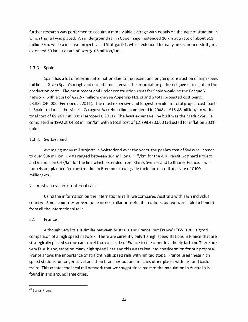
23
further research was performed to acquire a more viable average with details on the type of situation in
which the rail was placed. An underground rail in Copenhagen extended 16 km at a rate of about $15
million/km, while a massive project called Stuttgart21, which extended to many areas around Stuttgart,
extended 60 km at a rate of over $105 million/km.
1.3.3. Spain
Spain has a lot of relevant information due to the recent and ongoing construction of high speed
rail lines. Given Spain’s rough and mountainous terrain the information gathered gave us insight on the
production costs. The most recent and under construction costs for Spain would be the Basque Y
network, with a cost of €22.57 million/km(See Appendix H.1.2) and a total projected cost being
€3,882,040,000 (Ferropedia, 2011). The most expensive and longest corridor in total project cost, built
in Spain to date is the Madrid-Zaragoza-Barcelona line, completed in 2008 at €15.88 million/km with a
total cost of €9,861,480,000 (Ferropedia, 2011). The least expensive line built was the Madrid-Sevilla
completed in 1992 at €4.88 million/km with a total cost of €2,298,480,000 (adjusted for inflation 2001)
(ibid).
1.3.4. Switzerland
Averaging many rail projects in Switzerland over the years, the per km cost of Swiss rail comes
to over $36 million. Costs ranged between 164 million CHF33/km for the Alp Transit Gotthard Project
and 6.5 million CHF/km for the line which extended from Rhine, Switzerland to Rhone, France. Twin
tunnels are planned for construction in Bremmer to upgrade their current rail at a rate of €109
million/km.
2. Australia vs. international rails
Using the information on the international rails, we compared Australia with each individual
country. Some countries proved to be more similar or useful than others, but we were able to benefit
from all the international rails.
2.1. France
Although very little is similar between Australia and France, but France’s TGV is still a good
comparison of a high speed network. There are currently only 10 high speed stations in France that are
strategically placed so one can travel from one side of France to the other in a timely fashion. There are
very few, if any, stops on many high speed lines and this was taken into consideration for our proposal.
France shows the importance of straight high speed rails with limited stops. France used these high
speed stations for longer travel and then branches out and reaches other places with fast and basic
trains. This creates the ideal rail network that we sought since most of the population in Australia is
found in and around large cities.
33
Swiss Franc

24
2.2. Germany
There is a geographic analogy between Germany and Australia. All along the west coast of
Germany lie major cities (Dusseldorf, Frankfort, Kӧln, etc.), while Berlin (which contains the most
population by almost twice as much as the second highest) is located on the east side. There is a large
area of low populated cities, likely due to the Hartz Mountains which are located along the longitudal
center; similar to Australia’s low populated cities within the center of the country, where there is more
desert.
2.3. Great Britain
Great Britain is not very similar to Australia, but its lack of a high speed rail network and its
current high speed 2 proposal makes it a good case study to explore. Great Britain plans on connecting
its major cities with high speed rail lines, which is exactly what Australia desires and is researching.
Upon completion of the proposal, the rail lines and maps can provide useful information for the
Australian high speed proposal Furthermore, Great Britain provides the numerous stations (many of
which contain fewer than 20,000 people) demonstrating how having more stops, does not necessarily
make a rail network successful (See Appendix H).
2.4. Italy
Italy is much more densely populated than Australia; however, similarities can be seen between
the two countries. Italy is very densely populated in and around its major cities (Rome, Venice, Milan,
Naples, etc.), similar to Australia (See Appendix H.1.2). For this reason, the high speed rails in Italy can
be an excellent study for the creation of Australia’s high speed rail line.
2.5. Japan
At first glance, Japan appears to offers little similarity in terms of population density versus train
stations to Australia; however, a closer look proves otherwise. Japan is far more densely populated than
Australia, but what truly brings both countries on a similar playing field is the location of the populated
areas. Australia is a much bigger country than Japan, but much of its population is located along the
outer edges of the country, depicted in the population maps located in Appendix H. When comparing
this corridor of populations and disregarding the rest of the country that is unpopulated, Australia
becomes comparable to Japan. Once the mindset that Japan can be used to resemble the outer coast of
Australia, the methods the country uses to connect its populations with a mix of high speed and fast
speed trains can be analyzed and help form the basis of knowledge for the Australian rail network
proposal.
2.6. Spain
Spain, though a small country, has many similarities to Australia when looking at the
southeastern corridor of cities in Australia. When comparing Spain (504,030 km2) to Australia
(7,617,930 km2) as a whole, Spain only has 6.5% of the total area of Australia. However, when comparing

25
Spain to the populated states of Victoria (504,030 km2) and New South Wales (39,273 km
2), Spain is 60%
of the combined areas, making it more comparable. Additionally, looking at Spain’s longest high speed
line, Madrid-Zaragoza-Barcelona (621 km), compares with the direct distance of Melbourne to Sydney
(700 km) and Brisbane to Sydney (731). Conversely, looking at shorter distances such as, Madrid-
Valladolid (179 km) and Madrid-Toledo (20.8 km) becomes comparable with other shorter distances in
Australia such as, Canberra to Sydney (240 km) or Melbourne to Geelong (80 km). Similarities exist
between the Spain’s population distributions and Australia’s when focusing on southeastern coast.
Spain is populated throughout its coastal regions, where Australia also has similar dense populations.
After the completion of Spain’s first high speed rail line, Madrid-Sevilla (471km), a modal shift for
transportation occurred. Before the high speed rail line, travel between Madrid and Sevilla could be
broken down into airplane (33%), conventional train (14%), bus (15%), and automobile (60%)
transportation. After the completion of the Madrid-Sevilla AVE corridor, transportation percentages
drastically changed to airplane (4%), high speed train (52%), conventional train (2%), bus (8%) and
automobile (34%). Considering the modal shift of transportation after the implementation of high
speed rail (AVE) in Spain, Australia can expect to see a similar increase. Based off of this analysis we
could expect high speed rail to become the optimum choice of transportation for short and long
distance travels in Australia.
2.7. Switzerland
A visual comparison of the population density between Switzerland and Australia shows
locational similarities. Australia’s eastern coast holds many highly populated areas, from Cairns to
Melbourne, with well-populated Perth on the western coast, separated by near barren land.
Switzerland has a very densely populated northern side, from Neuchatel to St. Gallen, with Luҫano in the
south, separated by the Alps. There are still many cities that reside throughout the Alps, whereas
Australia’s outback contains very few cities. In both cases, these cities help connect the two areas of
heavy population, with some Swiss cities’ residency as low as 12,467 (Brig) having 4 direct-route
inbound/outbound connections.
2.8. US
The US is in a very similar situation as Australia. There are no high speed rails in the country, but
people are trying to fix this through the America2050 plan. The US and Australia both have a large
amount of land with people settled in only a few areas. It is said that the US has 11 “megaregions” in
which 70% of the total population resides and Australia has 5 major cities with about 55% of the
population (Todorovich & Hagler, 2011). Finally a helpful discovery that was made while making the US
proposal was that the most successful corridors are those that run from about 160-1000km while
connecting major employment centers with large population hubs (ibid).
3. Possible Upgrades/proposals
We created many different rail lines, but not all were used in our final proposal. After creating
different lines based on the information we had gathered from the international rails and Australia, we

26
began to look at the best possible rail network. For some connections there were not many options. As
seen in Figure 4, we designed 4 different routes between Melbourne and Adelaide, 3 between
Melbourne and Sydney and 2 between Sydney and Brisbane. Tables in Appendix H are charts containing
the total length of each track, the total population that is reached by each rail and the number of
stations/stops that would be needed. Using this information and the cost estimation (See Appendix H),
we were able to design the most desirable high speed rail for Australia.
Figure 4 High Speed Rail Proposal (Google Earth)
Once the high speed rail was finalized, we began to connect other cities to reach 80% of the
population. Following Japan’s lead, we create a rail network with a high connectivity (See Appendix C).
4. Limitations of Research
As with any project there are limitations and restrictions that need to be considered. Also, with
a time sensitive project some questions were not fully explored.
4.1. Information Acquisition
Most of the information we acquired or used in our project was obtained from the internet or
information BZE had given us. The information from the web was mainly from government websites,

27
but in some cases other websites were used. There is always a possibility that the information was not
sufficiently accurate. Also, some information was taken from work BZE had done, so there were no
other studies to support or reject its findings.
When it came to analyzing the information we had gathered, there were many factors that
could have been overlooked. For example, when we compared cost we had to take into consideration
inflation and currency conversions, but we also did not know if the cost of the materials had changed
from year to year and country to country.
4.2. Biases
In many studies, there lies a bias that must be overcome. The major bias that we had to overcome
in this study was being pro-rails. In our study we promoted the use of rails over all other methods of
transportation, but we could not overlook data claiming that rail use contains negative effects or that
other methods of transportation were better. Another bias was our focus on reaching 80% of the
population. If we were not working to reach 80% of the population, our results could have been
different depending on what our main focus was.

28
V. Conclusions and Recommendations
The information gathered on the international rail networks enabled us to construct a rail
network proposal for Australia. The proposal incorporated many of the aspects that other countries’ rail
networks contained: station location, high speed rail versus fast/basic rail, and how each rail line
operated trains of various speeds. Upon completion of the rail network, we were able to comprise a list
of recommendations to help provide a successful rail network for Australia.
A successful Australian rail network would look like the one in Figure 4. The common theme
found in every country with a
high speed rail network was
that all major cities should be
linked with a high speed rail,
minimizing stops between
major cities. Limiting the
amount of stops along a high
speed line is important
because the main purpose of
a high speed train is to get its
passengers from point A to
point B as quickly as possible;
more stops will increase the
travel time. The more popular
travel destinations in other
countries were also given a
high speed station, such as
Ueno, Japan (home of much of Tokyo’s cultural museums). This concept justified the allocation of a high
speed line running up to Cairns, a popular point of access to the Great Barrier Reef; thus, the main 6
cities for the high speed line of our proposal were Perth, Adelaide, Melbourne, Sydney, Brisbane, and
Cairns. Several lines could then be drawn, connecting city to city, creating the high speed line.
Figure 5 Australian Rail Network Proposal

29
There were not many options for high speed lines
from Perth to Adelaide, Sydney to Brisbane, and Brisbane
to Cairns; however, from Adelaide to Melbourne and from
Melbourne to Sydney, several options arose. We looked at
different routes between two major cities, looking for a
path that reached not only a large amount of the
population, but had limited stops, was relatively direct, and
avoided elevation peaks, due to mountains or lakes (more
costly than building over a flat surface). Once multiple
routes were mapped out, all of the aforementioned factors
were considered while applying an estimated cost analysis.
Weighing the different options, we decided on the chosen
routes seen in Figure 4. The path between Perth and
Adelaide was adjusted to avoid a reserve on the southern
coast. Although, there was an option with one fewer stop
for the route between Adelaide and Melbourne (Figure 5),
route 4, with 6 stops, was chosen over the other 3 options because, although it cost an estimated $16
million more than any of the other 3 options (See Appendix G), it reached the highest amount of
population, provided access to tourist attractions such as the various beaches in Victoria and the Great
Ocean Road, and had the least grade of slope34.
The route between Melbourne and
Sydney (Figure 6) was more complex; we made
three different possible routes and then had
two combination routes. The most direct route
that reached the highest amount of the
population and had the best elevation was
routes 1L and 1R which was chosen to connect
Melbourne and Sydney35. The final corridor
with different options was from Sydney to
Brisbane. Of the two options (which can be
observed in Appendix H.2.2) route 1 was the
best because, it was a shorter more direct,
reached a greater amount of the population,
and had the least grade of slope.
After implementation of the high speed
34
The grade of slope was calculated in GoogleEarth along every rail line to determine the
35 1
L and 1
R run through national reserves and will need to modified slightly
2L
1R
3 1L
2R
1
2
3
4
Figure 6 Adelaide to Melbourne Corridor
Figure 7 Melbourne – Sydney Corridor

30
line, the fast/basic speed lines were added to link up the towns surrounding the major cities36, and
provide the final 25% of Australia’s population with rail access. The rail maps of the other countries
provided insight on the paths of these other rail lines. Not only was it important to run rail lines radially
out of the major cities, but it was also important to provide rail lines perpendicular to these radial lines,
to form a grid within the rail network. These “crossing” lines were important to allow for the rail
network to provide better connectivity and allow for more options while traveling, especially for the
larger cities (50,000+ people).
The approximate cost of the high speed line was analyzed for several alternative paths.
Appendix G depicts 4 optimized pathways in terms of maximum coverage, minimum cost, minimum
stations and maximum distance. There was no one path that was best in all 4 qualities. These individual
paths were not chosen because a numerical optimization was not concluded to be the most effective
path; rather, an average was used in order to more effectively agree with the qualitative factors, such as
the reaching of tourist attractions.
The denser populated countries, such as Japan and Italy, proved useful in the creation of the
section of the rail network located between Melbourne and Brisbane, while the other less densely
populated countries helped for the creation of other corridors of the Australian rail network. Many
populated cities and towns are located between the Melbourne-Brisbane Corridor. With cities and
towns so centrally located, the rail network turned into a grid, as opposed to having a radial pattern.
Due to the numerous towns located within a small area, the grid patterns observed in the rail networks
of Italy and Japan (the more densely populated countries) acted as useful analogies. When a rail
network branches out from one city to reach 20+ towns, crossing lines between some of the further out
towns should be added to the network to allow for travel between the towns further away from the city.
The calculated connectivity of the other countries showed the importance of offering more connections
along the rail line. These, as well as that of the proposed network can be seen below in Figure 7.
36
~55% of the population
Figure 8 Rail Network Connectivity
31
Originally, the network had an average number of direct connections of approximately 1.5, meaning (on
average) every other station in Australia had one or two direct connections. Similarly, with Switzerland’s
current network, the 2.6 signifies the same situation but with two to three direct connections. With our
proposal, the new value is about 2.1, thus the average station has at least 2 direct connections. The
higher the connectivity of a rail network, the more destinations it can provide for its passengers, and the
more likely the rail network’s target population is to use the rail network (Kamba, O.K. Rahmat, & Ismail,
2007).
The rail network that we created requires further study and evaluation. Better software, in
addition to more time spent analyzing local topography, can be used to determine the actual paths for
the various rail lines. Additionally, the current rail lines throughout Australia can be compared with our
rail network to determine if there is any overlap or if there is a path already along or close to one of our
rail lines. This is especially important because it is cheaper to upgrade a rail line instead of building a
new one altogether, and, if there is already a rail line that cuts through a mountain, it could potentially
save more money to upgrade that rail line, instead of tunneling a new line (AECOM, 2011).
While the foundation of the rail network is important to its success (location of stations, type of
track, etc.), it is also important to consider the types of services provided along the rail lines. Studies
should be conducted to determine how often travel between the cities is required/desired. This
information is essential in determining how often to run trains along the rail lines. Regardless of how
often the trains run, we would recommend that the rail lines between the major cities run both high
speed and fast speed trains. Based on the methods of other countries, it may be extremely beneficial to
run a non-stop high speed train once per hour along the Melbourne-Sydney line, with another high
speed train and a fast speed train running semi-hourly, making stops at select stations and at all the
train stations along the line, respectively. This technique is utilized by Japan along its rail lines, and it is a
very efficient method of accommodating passengers who want to travel longer distances more quickly,
and those who desire to travel shorter distances. This method can be utilized along the fast/basic lines
as well, having a fast speed train run and stop at select stations, and a basic speed train running behind
it, stopping at all stations. The “select stops” that the fast speed train stops at can be determined by
further study of the travel patterns of Australians; identifying the most popular destinations along a
given line, and having those locations be the “select stops.” It is also important, if this method is used,
that the train that stops more frequently does not interfere with the high speed trains running behind
them or the high speed train will have to slow down and will lose its effectiveness.
With our proposal and our recommendations, Australia can have a well-developed rail network
that is accessible and successful, providing useful travel for both short and long distances. With a better
rail network, Australia can expect to see a shift from road to rail. This shift will lower the amount of
carbon emissions released by the transportation sector and in turn lower Australia’s carbon footprint,
reducing the effects of global warming.

32
Bibliography
AECOM. (2010). Mildura Rail Feasibility Study: Final Report. Melbourne.
AECOM. (2011). High Speed Rail Study: Phase 1. Sydney.
AFP. (2010, October 26). PHYSORG.com. Retrieved 2012, from German electric car sets new distance
record: http://www.physorg.com/news/2010-10-german-electric-car-distance.html
Agency, U. E. (2006). Greenhouse Gas Emissions from the U.S. Transportation Sector, 1990-2003. Fairfax:
IFC Consulting.
All facts and figures. (n.d.). Retrieved 2012, from European Commission Mobility & Transportation:
http://ec.europa.eu/transport/strategies/facts-and-figures/all-themes/index_en.htm
Arduin, J.-P., & Ni, J. (2005). French TGV Network Development. Japan Railway & Transportation Review,
22-28.
Association of Train Operating Companies. (n.d.). Retrieved 2012, from National Rail Enquiries:
nationalrail.co.uk
Beesley, M. (1965). The Value of Time Spent in Travelling: Some New Evidence. Economica, 32(126),
174-185.
Brinkhoff, T. (2012). Retrieved 2012, from City Population: http://www.citypopulation.de/
Burwell, D. (2010, April 15). Transportation—The Leading Cause of Global Warming. Retrieved 2011,
from Carnegie Endowment: For International Peace:
http://carnegieendowment.org/2010/04/15/transportation-leading-cause-of-global-
warming/afa
BZE. (2011). Where do Australians live? Melbourne, Victoria, Australia.
Carbon Dioxide Information Analysis Center (CDIAC). (n.d.). Frequently Asked Global Change Questions.
Retrieved 2012, from Carbon Dioxide Information Analysis Center:
http://cdiac.ornl.gov/pns/faq.html
Chefurka, P. (2007). How Much CO2 Do Electric Cars Produce? Retrieved 2012, from
http://www.paulchefurka.ca/Electric%20Cars%20and%20CO2.html
Climate Avenue. (2011, October 22). Retrieved 2012, from A New Era Of High Speed Rail Development:
www.climateavenue.com/high.speed.rail.index.htm
Coinnews Media Group LLC. (n.d.). US Inflation Calculator. Retrieved 2012, from
http://www.usinflationcalculator.com/

33
Department for Transport. (2012). Line of route. Retrieved 2012, from High speed rail:
http://www.dft.gov.uk/topics/high-speed-rail/line-of-route/
EPA. (n.d.). Retrieved from http://www.epa.gov/climatechange/emissions/co2.html
Ferropedia. (2011). Costos de construcction de infraestructura . Retrieved 2012, from Ferropedia:
http://www.ferropedia.es/wiki/Costos_de_construcci%C3%B3n_de_infraestructura#cite_note-
Tintin-0
Ferropedia. (2011). LAV Madrid - Sevilla. Retrieved 2012, from Ferropedia:
http://ferropedia.es/wiki/LAV_Madrid_-_Sevilla#Velocidades_autorizadas.
Ferropedia. (2012). LAV Madrid - Zaragoza - Barcelona. Retrieved 2012, from Ferropedia:
http://ferropedia.es/wiki/LAV_Madrid_-_Zaragoza_-_Barcelona
First ScotRail. (n.d.). Performance and Reliability. Retrieved 2012, from About ScotRail:
http://www.scotrail.co.uk/performance
Fischlowitz-Roberts, B. (n.d.). Earth Policy Institute. Retrieved 2012, from Carbon Emissions Climbing:
http://www.earth-policy.org/indicators/C52/carbon_emissions_2002
Gruppo Ferrovie. (2008). Frecciarossa: the new railway system that shortens distances. Retrieved 2012,
from Trenitalia:
http://www.trenitalia.com/cms/v/index.jsp?vgnextoid=38663bf7c819a110VgnVCM1000003f16f
90aRCRD
Gruppo Ferrovie. (2008). Our Trains. Retrieved 02 08, 2012, from TrenItalia:
http://www.trenitalia.com/cms/v/index.jsp?vgnextoid=38663bf7c819a110VgnVCM1000003f16f
90aRCRD
Gunther, M. (2011, April 20). How Much Does an Electric Car Really Cost? Retrieved 2012, from
GreenBiz.com: http://www.greenbiz.com/blog/2011/04/20/how-much-does-electric-car-really-
cost?page=0%2C1
Heidt, T. v., Gillett, P., Hale, C., Laird, P., Wardrop, A., Weatherby, R., et al. (2010). High-speed Rail:
Strategic information for the Australian context. Brisbane: CRC for Rail Innovation.
HS1. (n.d.). Retrieved 2012, from High Speed 1: http://highspeed1.co.uk/
Hunt, G. (1996). Results of Electric Vehicle Safety Issues Survey. Us Department of Energy.
I Want That Flight. (2011). Flights. Retrieved 02 06, 2012, from I Want That Flight:
http://iwantthatflight.com.au/General-
Links.aspx?ts=RESULTS_SUBMITTED&ti=12799644&rndx=85006858.16374217
IFEU. (2010). EcoPassenger: Environmental Methodology and Data. Heidelberg: International Union of
Railways (UIC).

34
Infrastructure. (2012, 1 24). Retrieved 2012, from Railway Technical Web Pages: http://www.railway-
technical.com/track.shtml
Internation Transport Forum. (2010). Transport and Innovation: Unleashing the Potential. Leipzig:
International Transport Forum.
International Rail Australasia . (n.d.). Trenitalia - Travel Italy by Rail. Retrieved 2012, from International
Rail: http://www.internationalrail.com.au/italy-by-rail.aspx
IPCC. (2007). Climate Change 2007: Synthesis Report. Retrieved 2012, from IPCC:
http://www.ipcc.ch/publications_and_data/ar4/syr/en/mains3-3-3.html
Jaffe, E. (2010, November 16). Five Reasons Electric Cars Will Have Trouble Catching On. Retrieved 2012,
from The Infrastructurist: http://www.infrastructurist.com/2010/11/16/five-reasons-electric-
cars-wont-catch-on/
Japan Area and Population. (n.d.). Retrieved 2012, from Worldwide-Tax: http://www.worldwide-
tax.com/japan/jappopulation.asp
Japan-Guide.com. (2012). Retrieved from Japan-guide.com: http://www.japan-guide.com/e/e2018.html
Kamba, A., O.K. Rahmat, A., & Ismail, A. (2007). Why Do People Use Their Cars: A Case Study in Malaysia.
Journal of Social Sciences(3), 117-122.
Kansas State University's Physical Activity and Public Health Laboratory. (2009, May 14). Survey research
looks at attitudes, obstacles to walking and biking to work. Women's Health Weekly, 335.
Levinson, D., Mathieu, J. M., Gillen, D., & Kanafani, A. (1997). The full cost of high-speed rail: an
engineering approach. The Annals of Regional science, 31: 189-215.
Live, J. (2010). The works already exceed more than one billion initial budget. elcomercio.
Low, N. (2008, 07 22). Melburnians want a better rail system. Let's make it happen. The Age, p. 2.
Ludewig, J., & Aliadiere, L. (2008, June). Rail Transport and Environment: Facts and Figures. Retrieved
2012, from UIC - International Union of Railways:
http://www.uic.org/homepage/railways&environment_facts&figures.pdf
Mackett, R. (2003). Why do people use their cars for short trips? Transportation, 329-349.
Madrid, E. . (2009, 07 25). El 41,3% de los ingresos de Renfe proceden ya del AVE. Retrieved 2012, from
Cinco Dias: http://www.cincodias.com/articulo/empresas/413-ingresos-renfe-proceden-
ave/20090725cdscdiemp_3/
Michaud, P. (1999, February 8). Infrared Radiation - Warmth From the Cold of Space. Retrieved 2012,
from Gemini: http://www.gemini.edu/public/infrared.html

35
Milmo, D. (2009, 08 05). Which country has the most high speed train lines? Retrieved 01 30, 2012, from
Guardian: http://www.guardian.co.uk/news/datablog/2009/aug/05/rail-transport-transport#_
Ministerio De Fomento. (2004). PLAN ESTRATÉGICODE DE INFRAESTRUCTURAS Y TRANSPORTE.
Minesterio de fomento.
Mong, A. (2010, 12 06). Japan to China: You've highjacked our high-speed rails. Retrieved 01 30, 2012,
from MSNBC: http://behindthewall.msnbc.msn.com/_news/2010/12/06/5597596-japan-to-
china-youve-hijacked-our-high-speed-rails
(n.d.). High Speed Rail in America.
(n.d.). Retrieved 2012, from Map of France: http://www.map-france.com/
(n.d.). Retrieved 2012, from Rail Saver:
http://www.firstgreatwestern.railsaver.co.uk/firstgreatwestern.htm
National Railroad Oassenger Corporation. (2012). Amtrak National Facts. Retrieved 2012, from Amtrak:
http://www.amtrak.com/servlet/ContentServer?c=Page&pagename=am%2FLayout&cid=12460
41980246
National Railroad Passenger Corporation. (2012). Retrieved 2012, from Amtrak: www.amtrak.com
Net Resources International. (2011). Retrieved 2012, from http://www.railway-technology.com/:
http://www.railway-technology.com/
Nye, B. (2011). The true value of rail. Barton: Deloitte.
OANDA. (2012). Historic Exchange Rates. Retrieved 2012, from OANDA:
http://www.oanda.com/currency/historical-rates/
Passengers - Timetables. (n.d.). Retrieved 2012, from Renfe:
http://www.renfe.com/EN/viajeros/horarios.html
Public Transportation Helps Protect Our Environment. (2011). American Public Transportation
Association.
Purcell, B. (2010). Getting Around Germany. Retrieved 2012, from Brian's Guide to Getting Around
Germany: http://www.gettingaroundgermany.info/index.shtml
Quarmby, D. (1967). Choice of travel mode for the journey to work: some findings. Journal of Transport
Economics and Policy, 273-314.
Rail Europe, Inc. (2012). Home. Retrieved 2012, from Rail Europe: http://www.raileurope.ca/index.html
RailCorp. (2005, May). Timetables. Retrieved 02 06, 2012, from NSW Transport: Country Link:
http://www.countrylink.info/book_your_trip/using_online_booking

36
Railsaver. (2010). First Great Western. Retrieved 2012, from Railsaver:
http://www.firstgreatwestern.railsaver.co.uk/firstgreatwestern.htm
Railway Finance. (2012, 1 24). Retrieved 2012, from Railway Techical Web Pages: http://www.railway-
technical.com/finance.shtml
Ramsey, M. (2010, October 17). High Battery Cost Curbs Electric Cars. Retrieved 2012, from The Wall
Street Journal:
http://online.wsj.com/article/SB10001424052748703735804575536242934528502.html
Renfe-Operadora. (2010). Punctuality Commitment. Retrieved 2012, from RENFE:
http://www.renfe.com/EN/viajeros/larga_distancia/servicios/serviciosCompromiso.html
Rogers, S., & Evan, L. (2011, January 31). World carbon dioxide emissions data by country: China speeds
ahead of the rest. Retrieved 2012, from The Guardian:
http://www.guardian.co.uk/news/datablog/2011/jan/31/world-carbon-dioxide-emissions-
country-data-co2
Rood, D. (2011, 08 04). $100 ticket to ride the high-speed rail to Sydney. Retrieved 02 06, 2012, from The
Age: http://www.theage.com.au/travel/travel-news/100-ticket-to-ride-the-highspeed-rail-to-
sydney-20110803-1ibp8.html
Rout, S. (n.d.). Limone sul Garda, Italy. Retrieved 02 08, 2012, from limone italy:
http://www.limoneitaly.com/
SBB. (2004). Key Figures. Retrieved 02 13, 2012, from SBB: http://www.sbb.ch/en/corporation/the-
company/key-figures.html
SBB CFF FFS. (n.d.). Online Timetables. Retrieved 2012, from SBB CFF FFS:
http://fahrplan.sbb.ch/bin/query.exe/en
Schafer, A., & Victor, D. G. (1998). Global passenger travel: implications for carbon dioxide emissions.
Retrieved from
http://www.uns.ethz.ch/edu/teach/bachelor/energmob/Schafer_Victor_1999.pdf
Smith, A. (2009). Money train: the cost of high speed rail. CNN.
Todorovich, P., & Hagler, Y. (2011). High Speed Rail in America. Lincoln Institute of Land Policy.
Torchbox. (n.d.). What are carbon emissions? Retrieved 2012, from The carbon account:
http://thecarbonaccount.com/carbonexplained/
Tourism Research Australia. (2011, 09). Travel by Australians. Retrieved 2012, from Department of
Resources, Energy, and Tourism:
http://www.ret.gov.au/tourism/Documents/tra/National%20Visitor%20Survey/travel-by-
australians-sept-quart-2011.pdf

37
Trading Economics. (2012). Rail Lines (Total Route-KM) in France. Retrieved 2012, from Trading
Economics: http://www.tradingeconomics.com/france/rail-lines-total-route-km-wb-data.html
World Resources Institute. (2008, 03 14). World Greenhouse Gas Emissions: 2000. Retrieved 2012, from
World Resources Institute: http://www.wri.org/chart/world-greenhouse-gas-emissions-2000
Wright, M., & Hearps, P. (2010). Australian Sustainable Energy: Zero Carbon Australia Stationary Energy
Plan. Melbourn: University of Melbourne Energy Research Institute.
ZVV. (2012). Online Timetable. Retrieved 2012, from ZVV:
http://online.fahrplan.zvv.ch/bin/query.exe/en

38
Appendix A: Glossary
Accessibility The rail network’s ability to provide its
passengers with access points and
destinations that fulfill their needs.
Carbon emissions Refers to carbon dioxide emissions. Carbon
dioxide released into the atmosphere due to
the use of energy, and absorbs and emits
radiation (EPA).
Connections The different directions one can go from a
given station.
Connectivity The average number of direct connections a
station provides (See Appendix C for further
detail).
Convenience The rail network’s ability to provide services
frequently throughout a daily operational
period that is able to fulfill passengers’ needs.
Cost Cost of building the rail lines which includes
the planning and land costs, infrastructure
building costs, and super structure costs.
Coverage The rail network’s accessibility to its
passengers and its ability to provide the
options of high speed (250+ km/h), fast (200-
250 km/h), or basic (<200 km/h) trains within
the city of the station or an adjacent city.
Frequency The interval at which a train departs from a
train station.
Track gauges The distance between the rails (inside rail to
inside rail).

39
Appendix B: Cost-Benefit Analysis
In a recent study on high-speed rail investment, a relation between costs and profitability was
found to be represented by the following:
∫ ( )
( ) ∫
∫ ( ) ( )
Where:
B(H) is the annual social benefits of the project. This may be economic or consumer
convenience (availability, etc.).
Q is the number of annual passenger-trips.
r is the social discount rate, which may be representative of changing living cost values or
depreciation due to age.
g is the annual growth of benefits and cost which depend on the level of real wages and Q.
I is the investment cost (construction, etc.).
Cf is the annual fixed maintenance and operations costs.
Cq(Q) is the annual maintenance & operating costs depending on Q (usage costs).
T is the total time of the high-speed rail project. For a permanent installment, we allow .
The equation has cleverly adopted the use of integrals and exponential functions instead of a
summation of yearly functions to allow for the incorporation of any instantaneous changes throughout
the functions.
The idea behind this equation should be straightforward; revenue should outweigh costs. It should
be noted that the investment costs seems to be a constant, but from an urban planning standpoint, it is
a complicated function in terms of track length, used land area and the type of track being used. It can
be written as shown below:
( ) ( )
Where
l is the rail length.
Cl is the cost-per-length of rail.
T(l,type) is the cost of landscaping the local terrain, as a function of the rail length and type of
terrain (mountain, etc.)
M(l) is other miscellaneous expenses as a function of track length, including train costs, station
establishment costs, etc.
The M(l) function was used to shorthand the many other possible time-independent expenses that
exist in establishing a high-speed rail. It should be noted that the terrain landscaping cost function is not

40
necessarily a linear function of length. For a quick reassuring example, it is easy to dig a hole, but it is
not easy to keep a larger hole from collapsing; this addition of length requires more work.

41
Appendix C: Connectivity
Background
The singular point in proving disconnectivity in the rail network, purely from a graph
theory standpoint, is that not every station connects to every other station. From a more
practical side, this is perfectly fine, as having every station do so would result in an
unnecessarily large number of lines required to be constructed. The following equation shows
the number of connections N resulting from a connected graph of n components.
∑
A rail network with 50 stations would have over 1200 lines! It would become the most
ideal state of a rail for accessibility, but it would be financially impossible. Therefore, any
feasible network proposition will require some stops for travelers. At this point, the question is
raised as to how disconnected can it be to still be successful?
Method
To begin, the connectivity of the Australian, German, Swiss and Japanese (the latter
three as a control [of “successful” networks]) rail networks are assessed. This is done by
categorizing the number of connections in/outbound direct connections of a station with the
number of stations that have such number. A single connection refers to a “dead-end” of a
track, two being a station that may serve as a stop along a singular path, and so forth. The
previously mentioned idealization is that each of the n stations have n-1 connections (connect
to all but itself). There is nothing wrong with having many stations with a lower number of
connections: this is because, in general, most cities will have a low population. As the
population increases, so should the number of connections to/from the city.
A Gaussian distribution equation can be found for the data set. The peak represents the
average number of connections of all the cities. Figure 9 shows the result for each case.

42
Figure 9 Initial Rail Network Connectivity
Limitations
There were two pitfalls throughout the development of this method.
The magnitudes of these curves cannot be the same unless the numbers of
stations are the same for all countries.
To fix this, percentages were used in either case. The dependent variable is therefore
“The percent of cities with said connections”, bringing the total integral of each case to 100.
This method assumes a somewhat even distribution of population distribution.
This is true; graph theory fails to acknowledge the effects of one or more components
having a very large distance from the larger portion of components. Such effects include issues
of cost, or overall efficiency or even worth of creating these connections. This can very readily
be observed in Australia, where most of the stations lie along the east coast, with Perth and
Darwin (west and north coast) having one to two connections. The outlying cities do have
somewhat comparable populations, but the fact remains that some of the stations lie in very
sparse cities.
To remedy the latter issue, a second sample of Australia was taken, this time excluding
Western Australia and Northern Territory, the lesser populated areas. Figure 10 shows the
percent total population by city-station connection, a relation which depicts evenness of
population density by number of connections. Switzerland has a relatively “nice” distribution,

43
with less total population on each end (least and most connections), with growing and decaying
population from the average of ~4.8 connections. As can be seen by Figure 10, the secondary
Australian sample was just as lacking in average connections.
Figure 10 Population Distribution by Connectivity
The width, as shown in Figure 10, is the best fit for the quantity √ , where is the standard
deviation of the Gaussian curve. Given that Switzerland can be agreed to have a much more
even population distribution than Australia, we can therefore attribute its larger width to such.
The smaller Australian sample has a larger width than the original and therefore has a more
even population distribution.
This secondary analysis is restricted by means of statistical theory. There was no data of cities
with seven or more connections in Australia, but the fit curves use the data and that side of the
Gaussian anyway. This “ghost” data is generated by nothing more than the idea that the
Gaussian curve is movable, as though one can figuratively translate the coordinate back and
forth across the connections axis, with each position its own relative population distribution
correlation. The idea is based off of the original relation seen in Figure 9, where the
coordinate has more meaning.
Conclusion
The stations in Australia (both overall and within the more populated region), Germany,
Switzerland and Japan (chosen due to their renowned success) were inventoried according to

44
number of in/outbound direct connections. It was shown that, on average, Australian stations
have one less connection than the other countries. Improvements made to this rail in regards
to accessibility should ideally move this average towards the right, implying that, on average,
Australians will have less of a hassle in getting from some points A to B, without making too
many intermediate stops.
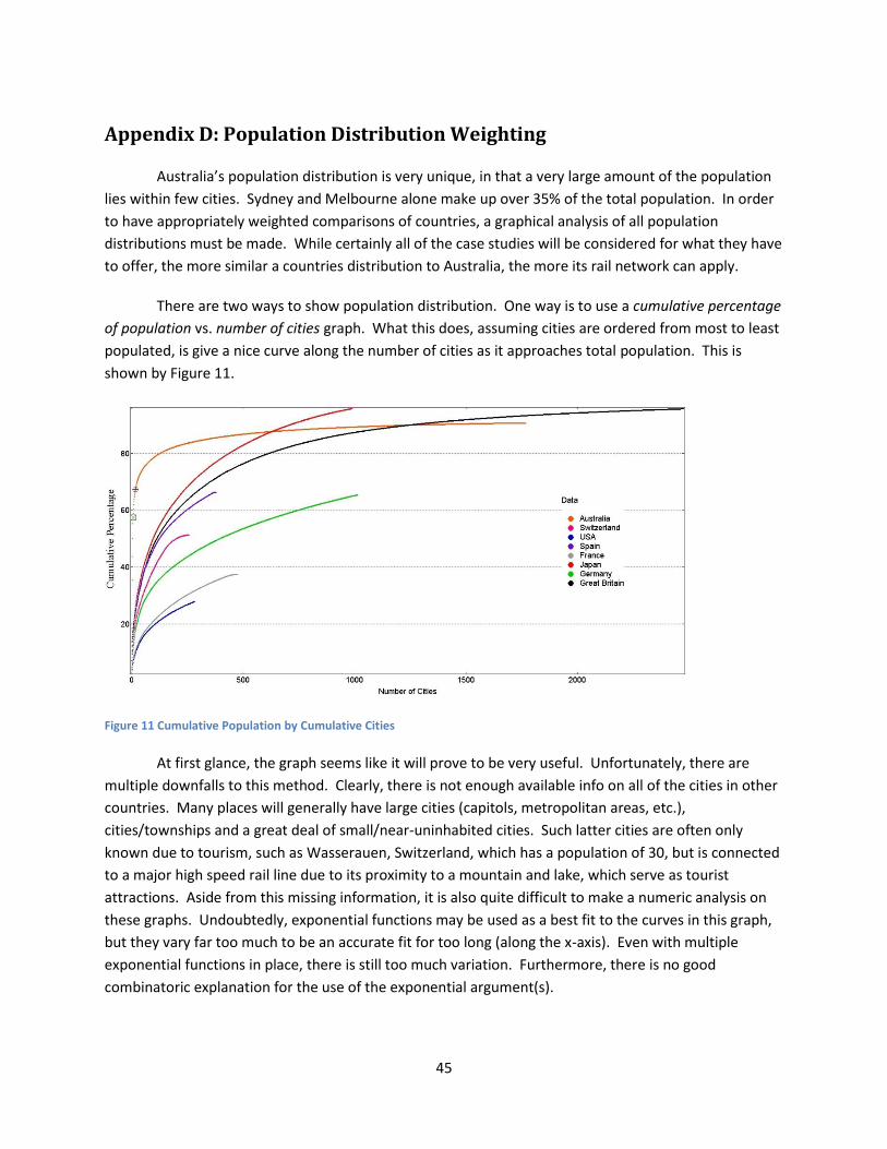
45
Appendix D: Population Distribution Weighting
Australia’s population distribution is very unique, in that a very large amount of the population
lies within few cities. Sydney and Melbourne alone make up over 35% of the total population. In order
to have appropriately weighted comparisons of countries, a graphical analysis of all population
distributions must be made. While certainly all of the case studies will be considered for what they have
to offer, the more similar a countries distribution to Australia, the more its rail network can apply.
There are two ways to show population distribution. One way is to use a cumulative percentage
of population vs. number of cities graph. What this does, assuming cities are ordered from most to least
populated, is give a nice curve along the number of cities as it approaches total population. This is
shown by Figure 11.
Figure 11 Cumulative Population by Cumulative Cities
At first glance, the graph seems like it will prove to be very useful. Unfortunately, there are
multiple downfalls to this method. Clearly, there is not enough available info on all of the cities in other
countries. Many places will generally have large cities (capitols, metropolitan areas, etc.),
cities/townships and a great deal of small/near-uninhabited cities. Such latter cities are often only
known due to tourism, such as Wasserauen, Switzerland, which has a population of 30, but is connected
to a major high speed rail line due to its proximity to a mountain and lake, which serve as tourist
attractions. Aside from this missing information, it is also quite difficult to make a numeric analysis on
these graphs. Undoubtedly, exponential functions may be used as a best fit to the curves in this graph,
but they vary far too much to be an accurate fit for too long (along the x-axis). Even with multiple
exponential functions in place, there is still too much variation. Furthermore, there is no good
combinatoric explanation for the use of the exponential argument(s).

46
The other way to display population distributions is to assign each city to belong to a particular
category of population. These categories must be carefully chosen to allow for an optimum
representation of the distribution; a logarithmic scale can be deceiving, and anything else non-linear
(such as an arbitrary list [10,000, 20,000, 50,000, etc.]) can misrepresent the population. Thus, the ideal
representation is to use percentiles for the categories.
The total population is divided into 1000 equal partitions. Each city is categorized into a
particular percentile, given by the ratio of the city’s population to the total. The populations of multiple
cities within a particular percentile are summed and a bar graph is created. Figures 12 and 13 show the
results for Australia and Great Britain.
Figure 12 Population Distribution by Percentiles - Australia

47
Figure 13 Population Distribution by Percentiles – Great Britain
Obviously, there is very little in common between Australia’s and Great Britain’s population
distribution. These two were chosen as the weighted average of all cities and their percentage of
population was closest, Australia at the 7.6757th percentile of its population and Great Britain at the
1.3151th percentile. All other cases’ weighted average remain underneath the first percentile. It is with
this numeric conclusion that one can justify by ratios of populations that Great Britain proves most
useful for comparison.
However, these percentiles do no justice for the corresponding populations. The 7.6757th
percentile of Australia is 1,523,883, meaning the average Australian lives in a city of said population.
The closest case study to this population is Japan, whose weighted average percentile of 0.94501th
corresponded to a population of 1,204,420. Interestingly enough, Japan was second to Great Britain in
average percentile, but vice versa in population (GB at 775,909). This allows for a more robust
conclusion that Great Britain and Japan are equally (if not somewhat more so Japan) suitable for
population-based comparisons. Table 1 below shows the weighting results for all of the cases.

48
Table 1 Comparison of International Population Distributions
Country Average Percentile Population Weighted Average Population
Australia 7.6757th 19853342 1,523,883
Great Britain 1.3151th 59000000 775,909
Japan 0.94501th 127450460 1,204,420
Spain 0.92018th 46081574 424,033
Switzerland 0.57042th 7825243 44,637
Italy 0.45691th 60600000 276,887
Germany 0.44580th 81702309 364,229
France 0.26662th 64876618 172,974

49
Appendix E: Locomotive Dynamics
The location of stations along the pathway of a rail network requires knowledge of what type of
train is being used. High speed trains would be inefficient if they cannot reach their maximum speed,
which will occur of the length of track between the stations is too short to allow the train to accelerate
enough.
The dynamics of train acceleration and deceleration can be derived from Newton’s Laws, given a
few experimental constants. Considering an accelerating train, the sum of all of the forces acting upon it
governs its inertia as a whole:
In this equation, m signifies the total mass of the train (hull, engine, crew, patrons, everything),
is the acceleration, is the gravitational force acting upon the train (which affects the acceleration
positively on downward slopes, and vice versa), is the aerodynamic drag force of the train, is the
friction force between the train and track, and is the tractive force of the engine pulling on the cars.
These parameters can be expanded given a couple of assumptions: the train is powered with an electric
current, and the velocity is high enough to use the high Reynold’s number interpretation of drag force
(this means the momentum transfer effect of the internal system [inside the train] is negligible
compared to the momentum of the external system [the train itself]).
( )
( ) ( )
( ) ( )
From here we make the following exemplary numeric assumptions (followed by sources of
assumptions):
(power of train) is 9 106 W (http://irsme.nic.in/files/FACT_RLY_ELC.pdf)
(efficiency coefficient) is 90% (http://www.easts.info/on-line/journal_06/278.pdf)
(mass) is 2.358 106 kg (http://www.irfca.org/docs/stats/stats-goods-train-load.html)
is 9.8067
(air density at 20 and 1 atm) is 1.2041
(unitless Drag coefficient of train) is 1.8 (http://www.engineeringtoolbox.com/drag-
coefficient-d_627.html)
(reference frontal area) is 11.5 m2
(http://www.scientificbulletin.upb.ro/rev_docs/arhiva/rez86368.pdf)
(unitless coefficient of friction) is 2.312 10-3 (http://www.inrets.fr/ur/lte/publi-
autresactions/fichesresultats/ficheartemis/non_road4/Artemis_del7b_rail.pdf)
(angle of slope) can be assumed to be zero (flat land). This only removes the basic term.

50
Assuming the initial state of the train to be at rest, this creates the following first order non-
linear initial value problem for velocity:
( )
(
), v(0) = 0
From this IVP, we can infer the trivial solution of ( ) ; as the train will start at remain at
rest, which nothing provoking the need for friction and drag forces. From here, we may apply Euler’s
method of linear approximation, which can be incorporated into a computer coded for-loop of iteration
i.
( ) ( ) ( )
( )(
( ) ( ) )
We can approximate the velocity of this model train recursively, point-by-point. Figure 14
shows the result of the previously mentioned code.
Figure 14 Approximate Acceleration of Locomotive

51
This exemplary motion of a high speed rail was calculated every 0.1 seconds for 45 minutes
(shown on x-axis). To avoid the error of dividing by zero, the initial velocity was adjusted to 0.1 m/s
(shown on y-axis converted to km/h).
This velocity curve not only gives a fine example of locomotive inertia based off of simple
Newtonian principles, but also depicts a valuable piece of information. Around 31 minutes is where the
train achieves the predefined “high speed” of 250 km/h. For a train with similar characteristics to this
example, it would be vital that the travel time is at least 31 minutes in order for the use of the train to
be worthwhile. Otherwise, it would be more cost effective to implement a basic or fast speed rail
system.
The deceleration of a locomotive undergoes identical forces with the exception of the tractive force. It is not assumed that the self-propulsion force simply goes to zero, as this would imply that the train simply allows itself to slow to a halt. This is by far not the case as emergencies would not be capable of being evaded (such as applying more brake in order to avoid a collision). Thus, we assume that a constant brake force is applied. The extrema magnitudes of this force would be zero (representing the previous situation) and that which is the limit of comfort to passengers, which we shall assume to have a value of 0.09 times the weight of the train (“Tractive Effort, Acceleration and braking”. The Mathematical Association 2004.). This changes our differential equation in the following way.
( ) ( )
( ) ( )
If we assume all previous experimental quantities, we acquire a new initial value problem, this time with
the boundary of v(0) =
(assuming the 300 km/h top speed of a high speed train [for longer timespan
of experiment] [given in m/s for the equation]). Figure 15 below is the result of the same approximation method.
Figure 15 Approximate Deceleration of Locomotive

52
The graph shows the limits of possibility for the train, signifying the lack of any brakes (red line) and the brakes with specified force (blue line). Certainly, with a stronger brake force, the lower limit decreases further, which on the scale of minutes approaches zero. With a more massive train and a smaller area of incidence, the upper limit increases variably. From a calculus standpoint, we know that the distance covered is equal to the integral of the velocity function over time, or:
∫ ( )
As the distance between the two stations certainly remain the same, the time will vary depending on how effective the velocity function is, which will essentially be a piecewise function. If is the total time of the trip, is the time to achieve top speed from zero (let us assume 250 km/h), and is the
time required for a safe, adequate deceleration to zero, then the velocity function throughout the trip will be as follows:
( ) {
( ) ( )
( ) ( )
The velocity function becomes more effective when and approach zero, allowing for the train
to travel at its top speed for as long as possible during the journey.

53
Appendix F: Travel Time Assessment
A study was made on local and non-stop (i.e. high speed) rail times for passengers between Los
Angeles and San Francisco. Its purpose is to relate factors which cause passengers to take the local
service rather than the non-stop service. This was achieved when the following equation was satisfied:
(
( )) (
( ))
Where
are the travel times for each service
is the schedule delay weighting coefficient (unitless constant denoting a circumstantial delay)
is the average time between the services
( ) is the difference between the literal clock time of the previous train of a service +
, and
the consumer’s target clock time S.
An oversimplification of this would be to use just travel times, which of course is
impossible as it would defeat the purpose of having a high-speed rail. Instead, the circumstance relies
upon how much of a delay the trains are accumulating.
Bearing this in mind, we immediately notice an issue with the equation: that there is ambiguity
between and ( ) of either side of the equation. Certainly they must differ as they relate to the delay
and train times of a single service.
While this relation may seem somewhat bare in terms of everything that adds to train time, it is
vague enough to allow for interpretation, as can be seen by the coefficient. Such interpretation may
even permit for the introduction of other modes of travel. For the purpose of the relation to our study,
we may rewrite parts of this equation, and arrive at the following.
( ) ( )
What is being observed with the satisfying of this equation is that the travel time by car, along with any
delay as a function of the car’s departure time S, ( ) (construction, traffic, etc.) is greater than the
travel time by high-speed rail, along with any delays as a function of the coordination between multiple
trains (train coordination, ticket purchase of the individual [assuming prepaid options are unavailable],
etc.), which relies on the departure time S, ( ).

54
Appendix G: Optimization of Parameters
The cost of construction for rail will vary depending on the type of terrain along the rail path.
The total cost per kilometer of Australian rail has been found for urban, tunneling, mountainous,
elevated, undulating and flat farmland implementation. For a general case for a path that may pass
through one or more of these area types, the cost (in millions of AUD $) equation would be as follows:
,
In this equation:
x1 denotes the length of track in the urban setting, where there is a clear sky-view of residential and commercial blocks, and the existence of a population for the area.
x2 is the length of tunneling track, utilized for rail segments that approach mountainous areas that vary in elevation with respect to distance too quickly to apply a gradient to the track, most especially for high speed rail.
x3 is the length of track upon mountainous terrain, which vary in elevation with respect to distance too quickly to apply slight (approximately zero) changes in track gradient, as seen in flat terrain.
x4 is the length of elevated track, used over distances containing large water bodies, and in some cases parks, and other sociopolitical boundaries that must be crossed over carefully.
x5 is the length of undulating track, defined as track that has an overall curve to it. As this does not apply directly to high speed (as high speed track should be as straightforward as possible when planning to be built), it is assumed this value will be low.
x6 is the length of track upon flat farmland, which has very small changes in elevation with relation to distance, and does not cross any body of water or park/urban boundaries.
Thus, for a non-zero route length, :
, and at least one of the components does not equal zero.
With no other boundary conditions, the trivial solution is to incorporate solely the flat farmland
setting in order to minimize cost. Unfortunately, this amount of ease implies that there is only flat
farmland everywhere between and around endpoints A and B of the path. This is simply untrue, as
there are indeed mountains within Australia, as well as heavily populated cities, rivers and areas which
are simply a hassle to build directly through. To apply the condition of reality to this problem, we
introduce the area function:
( ) ( )
Where X is the global longitude, Y is the latitude, E is the elevation of the location, T is the type
of geographical feature of the location (water, somewhat level land, mountain, etc.), and P is the
population of the area. What this relation implies is that for every global position, there is a determining
function of population, elevation and land-type that will govern the required area-type of track for that
location. This function is applied continuously throughout the path between the two points (generally
cities), and with thorough calculations, the magnitudes of can be found. From here a total cost is

55
acquired by using these magnitudes in the original cost equation; though this is simply one possible
path. A second path may be created by “tweaking” this path, perhaps simply applying a distortion in a
single direction, much like pulling back on a string of a guitar. Clearly this increases the magnitude of l,
which in turn will change , but this can be beneficial for reducing the total cost.
For example, let’s assume the path from City A to City B is 100 km, with mountain area between
30 and 60 km along the path. For simplicity, all other path will be flat farmland. This gives us a total
cost of $2906.68 million. However, if there exists a path around the mountain, such that it adds 50 km
to the path but causes the whole path to be farmland, the total cost becomes $1919.38 million for the
rail. This example is an extreme oversimplification of the topology in Australia; to the point where
coding is required to arrive at the same basic solution.
This brings us to the limitation of this method. The defined boundary function ( ) currently
does not exist in archival form for Australia, in a way that does not involve extensive budget options
surpassing that of the ability of the group, or programs which require a great deal of time-consuming
training.
Alternatives for routes were found during the creation of the high speed network to give a
discrete set of comparisons as seen in Figure 16. Four alternatives were made to connect Melbourne
and Adelaide, three between Sydney and Melbourne, and two between Brisbane and Sydney. The
alternatives were labeled in numerical order descending in global latitude.
Figure 16 Depiction of All Possibile Alternative High Speed Rail Lines

56
Table 2 below shows the analysis for coverage (the sum of the populations of cities expecting to
have a station in them throughout the line, as well adjacent cities to simulate proximity to the station),
the expected cost (roughly calculated by categorizing segments of the line to acquire the total ), the
number of expected stations throughout the line, and the total length of the line.
Table 2 Comparison of Optimized High Speed Lines
Path A: Highest
Coverage
Distance
(km) 69.73% Stations: 43
Route Distance Cumulative Pop Cost (millions)
Cost/km
(millions)
Brisbane - Cairns
1,528
699,817 29236.26959 19.13368429
Sydney - Brisbane 2
789
2,983,789 29070.79193 36.70554537
Melbourne - Sydney 1
836
4,205,020 31343.00664 37.44684186
Melbourne - Adelaide 4
795
3,571,610 20838.01724 26.21134244
Adelaide - Perth
2,425
2,383,281 53519.6924 22.06997625
Total
6,373
13,843,517 164007.7778
25.734784
Path B: Lowest Cost Coverage: 68.77% Stations: 45
Route
Distance
(km) Cumulative Pop Cost (millions)
Cost/km
(millions)
Brisbane - Cairns
1,528
699,817 29236.26959 19.13368429
Sydney - Brisbane 2
789
2,983,789 29070.79193 36.70554537

57
Melbourne - Sydney 3
791
4,042,691 29837.14147 37.62565129
Melbourne - Adelaide 1
820
3,543,018 15081.08407 18.36916452
Adelaide - Perth
2,425
2,383,281 53519.6924 22.06997625
Total
6,353
13,652,596 156744.9795
24.672592
Path C: Least Stops Coverage: 69.07% Stations: 39
Route
Distance
(km) Cumulative Pop Cost (millions)
Cost/km
(millions)
Brisbane - Cairns
1,528
699,817 29236.26959 19.13368429
Sydney - Brisbane 2
789
2,983,789 29070.79193 36.70554537
Melbourne - Sydney 2
721
4,102,667 40160.17853 55.62351597
Melbourne - Adelaide 1
820
3,543,018 15081.08407 18.36916452
Adelaide - Perth
2,425
2,383,281 53519.6924 22.06997625
Total
6,283
13,712,572 167068.0165
26.590485
Path D: Most Distance Coverage: 69.39% Stations: 43
Route
Distance
(km) Cumulative Pop Cost (millions)
Cost/km
(millions)
Brisbane - Cairns
1,528
699,817 29236.26959 19.13368429

58
Sydney - Brisbane 1
861
2,945,168 54718.10552 63.33114065
Melbourne - Sydney 1
836
4,205,020 31343.00664 37.44684186
Melbourne - Adelaide 1
820
3,543,018 15081.08407 18.36916452
Adelaide - Perth
2,425
2,383,281 53519.6924 22.06997625
Total
6,470
13,776,304 183898.1582
28.423208

59
Appendix H: Findings
H.1. International Rails
H.1.1. Populations and Station Locations
Figure 17 Elevation Profile (left) and Population Density (right) for France with Rail Map
Table 3 Population of Cities/Towns in France with Stations
City Population 1/1/09 Track Type
Mont Saint Michel*
42 Non-Electrified
Chantes*
106 Non-Electrified
Merrey*
134 Normal Speed
Blesme*
178 Normal Speed
Fos*
253 Normal Speed
Lapeyrouse*
295 Non-Electrified
Lison*
475 Normal Speed
Peyraud*
504 Normal Speed
Hombourg Budange*
508 Normal Speed
Monterolier*
517 Normal Speed
Saint Exupery* Normal Speed

60
537
Courtalain*
595 Normal Speed
Chemilly*
630 Non-Electrified
Abancourt*
653 Normal Speed
Amagne-Lucquy*
689 Normal Speed
Motteville*
730 Normal Speed
Aspres-sur-Buëch *
752 Non-Electrified
Saint Maixent*
754 Normal Speed
Folligny*
941 Non-Electrified
Apach*
943 Normal Speed
Siorac-en-Périgord*
994 Non-Electrified
Estivareilles*
1,008 Non-Electrified
Serqueux*
1,061 Normal Speed
Puyoo*
1,150 Normal Speed
Mouchard*
1,188 Normal Speed
Béning-lès-Saint-Avold*
1,226 Normal Speed
Bréauté *
1,236 Normal Speed
Lérouville *
1,473 Normal Speed
Rothau*
1,582 Non-Electrified
Briouze*
1,600 Non-Electrified
Longueville*
1,625 Non-Electrified
Saint Florent*
1,635 Non-Electrified
Aillevillers-et-Lyaumont *
1,653 Non-Electrified
Arches*
1,726 Normal Speed

61
Crépy *
1,832 Normal Speed
Gièvres*
2,189 Normal Speed
Serquigny*
2,204 Normal Speed
Lauterbourg*
2,216 Non-Electrified
Saint Amour*
2,247 Normal Speed
Volgelsheim*
2,322 Non-Electrified
Saint-André-le-Gaz*
2,327 Normal Speed
Saint Germain*
2,351 Normal Speed
Nexon*
2,412 Non-Electrified
Conflans-en-Jarnisy*
2,446 Normal Speed
Lusignan*
2,637 Normal Speed
Chalindrey*
2,706 Normal Speed
Montréjeau *
2,722 Normal Speed
Gilly-sur-Isère*
2,798 Non-Electrified
Connerré*
2,872 Normal Speed
Aunay-sur-Odon*
2,944 Non-Electrified
Culoz*
2,957 Normal Speed
Carnoules*
3,162 Normal Speed
Veynes*
3,168 Non-Electrified
Modane*
3,472 Fast Speed
Contrexéville*
3,526 Non-Electrified
Saint-Germain-des-Fossés*
3,672 Normal Speed
Montmélian*
3,933 Normal Speed
Pontorson* Non-Electrified

62
4,094
Bouzonville*
4,178 Normal Speed
Villars Les Dombes*
4,317 Non-Electrified
Moret-sur-Loing*
4,472 Normal Speed
Morcenx*
4,586 Normal Speed
Volvic*
4,606 Non-Electrified
Mézidon-Canon*
4,683 Normal Speed
Dol-de-Bretagne*
4,807 Normal Speed
La Voulte-sur-Rhône*
4,993 Normal Speed
Santes*
5,036 Non-Electrified
Saint Rambert d'Albon*
5,198 Normal Speed
Flers-en-Escrebieux*
5,342 Non-Electrified
Chagny*
5,391 Normal Speed
Montchanin*
5,505 Non-Electrified
Montbard*
5,554 Fast Speed
Vendenheim*
5,646 Normal Speed
Longuyon*
5,711 Normal Speed
Salbris*
5,766 Normal Speed
Gannat*
5,881 Non-Electrified
Mirecourt*
5,956 Non-Electrified
Malesherbes*
6,015 Normal Speed
Bellegarde*
6,202 Normal Speed
Carentan*
6,340 Normal Speed
Givet*
6,777 Non-Electrified

63
Savenay*
7,039 Normal Speed
Elne*
7,452 Normal Speed
Saint Sulpice-Lauriere*
7,612 Normal Speed
Guingamp*
7,661 Fast Speed
Saint Marcellin*
7,794 Non-Electrified
Moirans*
7,804 Normal Speed
Coutras*
7,815 Normal Speed
Avranches*
8,226 Non-Electrified
Lure*
8,263 Non-Electrified
Rivesaltes*
8,625 Normal Speed
Livron-sur-Drôme*
8,945 Normal Speed
Paray-le-Monial *
9,138 Non-Electrified
Hagondange*
9,212 Normal Speed
Molsheim*
9,331 Non-Electrified
Dourdan*
9,435 Normal Speed
Hirson*
9,473 Normal Speed
Redon*
9,493 Fast Speed
Saint Gaudens*
11,152 Normal Speed
Lamballe*
11,261 Normal Speed
Gisors*
11,677 Normal Speed
Arachon*
11,679 Fast Speed
Auray*
12,435 Normal Speed
Ambérieu-en-Bugey*
12,696 Normal Speed
Granville* Non-Electrified

64
13,100
Tarascon*
13,177 Normal Speed
Bayeux*
13,478 Normal Speed
Argentan*
14,642 Non-Electrified
Tergnier*
14,722 Normal Speed
Les Herbiers*
14,893 Non-Electrified
Landerneau*
14,902 Normal Speed
Lourdes*
15,254 Fast Speed
Saint Pierre-des-Corps*
15,370 Normal Speed
Gien*
15,447 Normal Speed
Morlaix*
15,605 Normal Speed
Montargis*
15,755 Normal Speed
Vesoul*
15,920 Non-Electrified
Toul*
16,230 Normal Speed
La Baule*
16,719 Fast Speed
Montereau-Fault-Yonne*
16,802 Normal Speed
Firminy*
17,569 Normal Speed
Selestat*
19,303 Normal Speed
Givors*
19,345 Normal Speed
Montceau-les-Mines*
19,548 Non-Electrified
Moulins*
19,837 Normal Speed
Lunéville*
19,937 Normal Speed
Cahors*
19,948 Normal Speed
Dax
21,003 Fast Speed

65
Forbach
21,595 High Speed
Lisieux
21,826 Normal Speed
Sainte Foy lès Lyon
22,015 Non-Electrified
Beaune
22,516 Fast Speed
Le Creusot
22,840 High Speed
Chaumont
23,411 Non-Electrified
Libourne
23,830 Fast Speed
Agde
24,031 Normal Speed
Épernay
24,317 Normal Speed
Dole
24,906 Fast Speed
Vichy
25,090 Normal Speed
Biarritz
25,397 Normal Speed
Miramas
25,440 Normal Speed
Laon
26,094 Non-Electrified
Saint Dizier
26,112 Normal Speed
Saintes
26,335 Non-Electrified
Aix-les-Bains
26,819 Fast Speed
Vierzon
27,020 Normal Speed
Alençon
27,325 Non-Electrified
Saumur
28,070 Normal Speed
Soissons
28,471 Non-Electrified
Orange
28,990 Fast Speed
Périgueux
29,273 Non-Electrified
Périgueux Non-Electrified
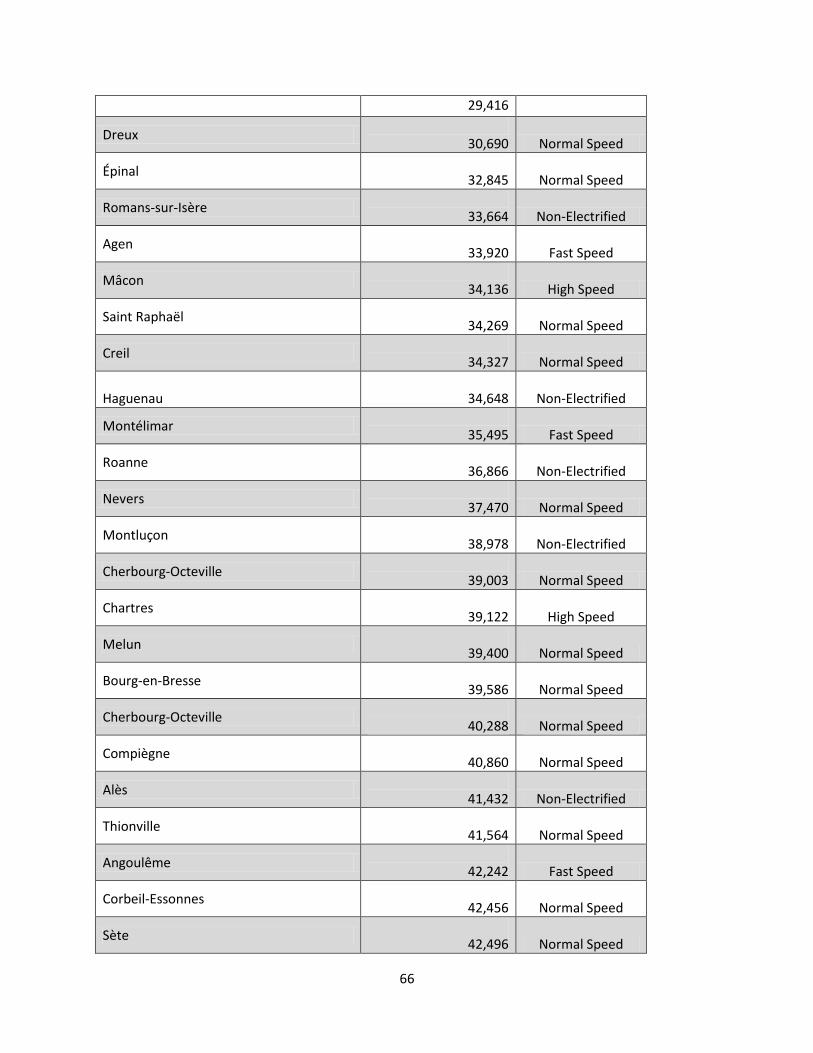
66
29,416
Dreux
30,690 Normal Speed
Épinal
32,845 Normal Speed
Romans-sur-Isère
33,664 Non-Electrified
Agen
33,920 Fast Speed
Mâcon
34,136 High Speed
Saint Raphaël
34,269 Normal Speed
Creil
34,327 Normal Speed
Haguenau
34,648 Non-Electrified
Montélimar
35,495 Fast Speed
Roanne
36,866 Non-Electrified
Nevers
37,470 Normal Speed
Montluçon
38,978 Non-Electrified
Cherbourg-Octeville
39,003 Normal Speed
Chartres
39,122 High Speed
Melun
39,400 Normal Speed
Bourg-en-Bresse
39,586 Normal Speed
Cherbourg-Octeville
40,288 Normal Speed
Compiègne
40,860 Normal Speed
Alès
41,432 Non-Electrified
Thionville
41,564 Normal Speed
Angoulême
42,242 Fast Speed
Corbeil-Essonnes
42,456 Normal Speed
Sète
42,496 Normal Speed

67
Mantes-la-Jolie
43,128 Normal Speed
Boulogne-sur-Mer
43,310 Normal Speed
Tarbes
43,686 Fast Speed
Bayonne
44,900 Fast Speed
Chalon-sur-Saône
45,504 Fast Speed
Saint-Brieuc
46,013 Fast Speed
Blois
46,013 Normal Speed
Châlons-en-Champagne(Châlons-sur-Marne)
46,236 Normal Speed
Saint Malo
47,045 Normal Speed
Carcassonne
47,854 Normal Speed
Brive-la-Gaillarde
49,231 Normal Speed
Charleville-Mézières
49,975 Normal Speed
Belfort
50,199 Normal Speed
Laval
51,182 Fast Speed
Évreux
51,193 Normal Speed
Narbonne
51,227 Fast Speed
La Roche-sur-Yon
52,234 Normal Speed
Vannes
52,683 Fast Speed
Arles
52,979 Fast Speed
Beauvais
54,461 Normal Speed
Saint Quentin
55,971 Normal Speed
Montauban
56,126 Fast Speed
Chambéry
56,476 Fast Speed
Niort Fast Speed

68
56,878
Lorient
57,812 Fast Speed
Troyes
61,188 Non-Electrified
Quimper
63,387 Fast Speed
Valence
64,364 Normal Speed
Saint Nazaire
66,348 Normal Speed
Bourges
66,786 Normal Speed
Colmar
67,214 Normal Speed
Béziers
70,957 Fast Speed
Cannes
73,372 Normal Speed
Calais
74,336 High Speed
La Rochelle
74,707 Normal Speed
Pau
82,763 Fast Speed
Poitiers
88,795 Fast Speed
Avignon
89,592 Fast Speed
Tourcoing
92,389 Normal Speed
Nancy
106,318 Fast Speed
Caen
109,312 Normal Speed
Rouen
110,688 Fast Speed
Mulhouse
111,156 Normal Speed
Orléans
113,224 Normal Speed
Besançon
117,392 Normal Speed
Perpignan
117,905 Normal Speed
Metz
121,841 Normal Speed

69
Amiens
133,998 Normal Speed
Tours
135,218 High Speed
Clermont-Ferrand
138,588 Normal Speed
Limoges
139,216 Normal Speed
Nîmes
140,747 Fast Speed
Brest
141,315 Fast Speed
Aix-en-Provence
141,895 Non-Electrified
Le Mans
142,281 High Speed
Angers
147,305 Fast Speed
Dijon
152,110 Fast Speed
Grenoble
155,632 Fast Speed
Toulon
165,514 Normal Speed
Saint Étienne
171,961 Fast Speed
Le Havre
177,259 Normal Speed
Reims
180,842 Non-Electrified
Rennes
206,604 Fast Speed
Lille
226,827 High Speed
Bordeaux
236,725 Fast Speed
Montpellier
255,080 Fast Speed
Annecy
255,771 Fast Speed
Strasbourg
271,708 Fast Speed
Nantes
282,047 Fast Speed
Nice
340,735 Normal Speed
Toullouse Fast Speed

70
440,204
Lyon
479,803 Fast Speed
Marseille
850,602 High Speed
Paris
2,234,105 High Speed
Table 4 Summary of Coverage for France
Population With Station in City 13,593,855
Total Population of France* 64,876,618
% Population in city of station 20.95%
Total Rail (km) (Trading Economics, 2012) 33,778
* Population from 2007 (Map of France)
(Brinkhoff, 2012)
Figure 18 Elevation Profile (left) and Population Density (right) for Germany with Rail Map
Table 5 Population of Cities/Towns in Germany with Stations
Station-Cities Pop. 12-31-2010 Rail Speed(s)
Cochem 4,929 High

71
Station-Cities Pop. 12-31-2010 Rail Speed(s)
Binz 5,407 High
Berchtesgaden 7,597 High
Barth 8,733 Non-Ev
Sassnitz 10,366 High
Pasewalk 11,319 High/Non-Ev
Buchloe 12,104 Non-Ev
Ludwigslust 12,319 High/Non-Ev
Plattling 12,746 High/Non-Ev
Treuchtlingen 12,778 High
Bebra 13,789 High
Füssen 14,213 Non-Ev
Angermünde 14,360 High
Sylt 15,169 Non-Ev
Bad Bentheim 15,567 High
Wittenberge 18,571 High/Non-Ev
Heide 20,886 Non-Ev
Neustrelitz 21,207 High/Non-Ev
Meiningen 21,590 Non-Ev
Husum 22,084 Non-Ev
Schleswig 24,058 High
Lindau (Bodensee) 24,772 High/Non-Ev
Norden 25,116 High/Non-Ev

72
Station-Cities Pop. 12-31-2010 Rail Speed(s)
Garmisch-Partenkirchen 26,068 High
Zittau 28,212 Non-Ev
Emmerich 29,571 High
Riesa 34,013 High
Uelzen 34,250 High/Non-Ev
Naumburg (Saale) 34,294 High/Non-Ev
Leer (Ostfriesland) 34,301 High
Kehl 34,789 High
Siegburg 39,746 High
Ansbach 40,253 High
Bautzen (Budyšin) 40,573 Non-Ev
Freiberg 41,342 High/Non-Ev
Stendal 42,435 High/Non-Ev
Rottenburg (am Neckar) 42,501 Non-Ev
Halberstadt 42,605 Non-Ev
Singen (Hohentwiel) 45,826 High
Hof 46,286 High/Non-Ev
Cuxhaven 50,492 Non-Ev
Passau 50,594 High/Non-Ev
Emden 51,616 High
Görlitz 55,596 Non-Ev
Stralsund 57,670 High

73
Station-Cities Pop. 12-31-2010 Rail Speed(s)
Offenburg 59,215 High
Rosenheim 61,299 High/Non-Ev
Kempten (Allgäu) 62,060 Non-Ev
Landshut 63,258 High/Non-Ev
Fulda 64,349 High/Non-Ev
Neubrandenburg 65,282 High/Non-Ev
Celle 70,242 High/Non-Ev
Bayreuth 72,683 Non-Ev
Lüneburg 72,983 High/Non-Ev
Rheine 76,530 High
Neumünster 76,830 High/Non-Ev
Gießen 77,366 High/Non-Ev
Marburg 80,656 High
Wilhelmshaven 81,324 Non-Ev
Dessau (-Roßlau) 86,906 High/Non-Ev
Flensburg 88,759 High/Non-Ev
Zwickau 93,750 High/Non-Ev
Schwerin 95,220 High/Non-Ev
Cottbus (Chóśebuz) 102,091 High/Non-Ev
Jena 105,129 High/Non-Ev
Trier 105,260 High
Koblenz 106,417 High

74
Station-Cities Pop. 12-31-2010 Rail Speed(s)
Bremerhaven 113,366 High/Non-Ev
Fürth 114,628 High/Non-Ev
Göttingen 121,060 High/Non-Ev
Wolfsburg 121,451 High
Ulm 122,801 High/Non-Ev
Ingolstadt 125,088 High/Non-Ev
Würzburg 133,799 High
Regensburg 135,520 High/Non-Ev
Darmstadt 144,402 High/Non-Ev
Heidelberg 147,312 High
Potsdam 156,906 High
Oldenburg (Oldenburg) 162,173 High/Non-Ev
Osnabrück 164,119 High/Non-Ev
Saarbrücken 175,741 High
Hagen 188,529 High/Non-Ev
Kassel 195,530 High/Non-Ev
Mainz 199,237 High/Non-Ev
Rostock 202,735 High/Non-Ev
Erfurt 204,994 High
Lübeck 210,232 High/Non-Ev
Magdeburg 231,525 High/Non-Ev
Halle (Saale) 232,963 High/Non-Ev

75
Station-Cities Pop. 12-31-2010 Rail Speed(s)
Kiel 239,526 High/Non-Ev
Chemnitz 243,248 High/Non-Ev
Braunschweig
[Brunswick] 248,867 High/Non-Ev
Mönchengladbach 257,993 High
Aachen [Aix-la-Chapelle] 258,664 High
Augsburg 264,708 High/Non-Ev
Münster 279,803 High/Non-Ev
Karlsruhe 294,761 High
Mannheim 313,174 High
Wuppertal 349,721 High
Duisburg 489,559 High
Nürnberg [Nuremberg] 505,664 High/Non-Ev
Hannover [Hanover] 522,686 High
Leipzig 522,883 High
Dresden 523,058 High
Bremen 547,340 High
Essen 574,635 High
Dortmund 580,444 High/Non-Ev
Düsseldorf [Dusseldorf] 588,735 High
Stuttgart 606,588 High/Non-Ev
Frankfurt (am Main) 679,664 High

76
Station-Cities Pop. 12-31-2010 Rail Speed(s)
Köln [Cologne] 1,007,119 High/Non-Ev
München [Munich] 1,353,186 High
Hamburg 1,786,448 High/Non-Ev
Berlin 3,460,725 High
Table 6 Summary of Coverage for Germany
Total Population of Cities/Towns with Stations 23,123,632
Total Population 81,702,309
% Population Located within Cities/Towns with Stations 28.30%
Total Rail (km) 33,706
(Brinkhoff, 2012)
Figure 19 Elevation Profile (left) and Population Density (right) for Great Britain with Rail Map

77
Table 7 Population of Cities/Towns in Great Britain with Stations
Cities/Towns with Stations Population Rail Type
Kyle of Lochalsh 660 ScotRail
Chapelton 760 First Great Western
Mallaig 760 ScotRail
Bridgend 790 Arriva Trains Wales/First Great Western
Carstairs 820 ScotRail
Dunlop 920 ScotRail
Langbank 930 ScotRail
Springfield 940 ScotRail
Newtonmore 1,060 ScotRail/East Coast
Hillside 1,140 Merseyrail
North Queensferry 1,150 ScotRail
Garelochhead 1,170 ScotRail
Brora 1,180 ScotRail
Dunkeld and Birnam 1,220 ScotRail/East Coast
Beauly 1,250 ScotRail
Croy 1,280 ScotRail
Kingussie 1,340 ScotRail/East Coast
Golspie 1,380 ScotRail
Balloch 1,430 ScotRail
Fairlie 1,530 ScotRail
Wylam 1,549 ScotRail/Northern

78
Cities/Towns with Stations Population Rail Type
Busby 1,550 ScotRail
Ladybank 1,560 ScotRail/Cross Country
Feniton 1,567 South West Trains
East Dean 1,578 South West Trains
Manea 1,579 East Midlands/Cnational Express East Anglia
Barnetby le Wold 1,593 Northern/East Midlands Trains
Great Bentley 1,613 National Express East Anglia
Howwood 1,620 ScotRail
Acton 1,635 First Great Western
Flimby 1,636 Northern
Meldreth 1,641 First Capital Connect
Hampton in Arden 1,655 London Midland
Ashwell 1,660 First Capital Connect
Blackridge 1,680 ScotRail
Ambergate / Crich 1,682 East Midlands Trains
Mistley 1,684 National Express East Anglia
Roche 1,685 First Great Western
Brompton (nr Northallerton) 1,690 Southern/London Overground
Aberdour 1,700 ScotRail
Llandeilo 1,731 Arriva Trains Wales
Seascale 1,747 Northern
Johnston 1,778 Arriva Trains Wales

79
Cities/Towns with Stations Population Rail Type
Starcross 1,780 First Great Western/CrossCountry
Brading 1,794 South West Trains
Barlaston 1,805 East Midlands Trains
Criccieth 1,826 Arriva Trains Wales
Kirkby Stephen 1,832 Northern
Thornton Dale 1,845 Northern
Swineshead 1,849 East Midlands
Narberth 1,869 Arriva Trains Wales
Kirknewton 1,880 ScotRail
Radley 1,906 First Great Western
Gartcosh 1,950 ScotRail
Wainfleet All Saints 1,965 East Midlands
Insch 1,970 ScotRail
Robertsbridge 1,987 Southeastern
Goxhill 1,994 Northern
Sleights 1,995 Northern
Hutton Cranswick 2,015 Northern
Goostrey 2,029 Northern
Sanquhar 2,030 ScotRail
Penrhyndeudraeth 2,031 Arriva Trains Wales
Watlington (King's Lynn and West
Norfolk)
2,031
First Capital Connect/National Express East Anglia

80
Cities/Towns with Stations Population Rail Type
Betws 2,034 Arriva Trains Wales
Invergowrie 2,040 ScotRail
Tisbury 2,041 South West Trains
Seamer(Scarborough) 2,048 Northern/First Transpennine Express
Westham 2,061 Southern
Wye 2,066 Southeastern
King's Sutton 2,069 First Great Western/Chiltern Railways
Kintbury 2,086 First Great Western
Lowdham 2,089 East Midlands Trains
Kirkconnel 2,090 ScotRail
Caldercruix 2,140 ScotRail
Machynlleth 2,147 Arriva Trains Wales
Cardross 2,170 ScotRail
Nafferton 2,184 Northern
Muir of Ord 2,190 ScotRail
Widdrington Station 2,197 Northern
Cromford / Matlock Bath 2,202 East Midlands Trains
Wickham Market 2,204 National Express East Anglia
Newport (Uttlesford) 2,208 National Express Anglia
Acle 2,230 National Express East Anglia
Wool 2,234 South West Trains
Llandovery 2,235 Arriva Trains Wales

81
Cities/Towns with Stations Population Rail Type
Bugle / Stenalees 2,243 First Great Western
Hightown 2,247 Merseyrail
Barmouth 2,251 Arriva Trains Wales
Elsenham 2,252 National Express Anglia
Watton-at-Stone 2,272 First Capital Connect
Sway 2,294 South West Trains
Arnside 2,301 Northern/First Transpennine Express
Carfin 2,310 ScotRail
Harlington 2,322 First Great Western
Renton 2,350 ScotRail
Lingwood 2,374 National Express East Anglia
Aspatria 2,376 Northern
Penmaenmawr 2,403 Arriva Trains Wales/Virgin Trains
Long Hanborough 2,404 First Great Western
Marden 2,412 Southeastern
Valley 2,413 Arriva Trains Wales/Virgin Trains
Greenfield 2,419 Northern
Markinch 2,420 ScotRail/Cross Country
Markinch 2,420 ScotRail/Cross Country
Laurencekirk 2,440 ScotRail
Longniddry 2,450 ScotRail
Shipton-under-Wychwood 2,480 First Great Western

82
Cities/Towns with Stations Population Rail Type
Gilfach Goch 2,504 Arriva Trains Wales
St Columb Road 2,510 First Great Western
Rolleston 2,545 East Midlands Trains
Wemyss Bay 2,550 ScotRail
Barrow upon Humber 2,554 Nothern
Wareham 2,568 South West Trains
Collingham(Nottinghamshire) 2,580 East Midlands Trains/East Coast
Lostwithiel 2,602 First Great Western
Bosham 2,604 Southern
Willington (South Derbyshire) 2,604 CrossCountry
Healing 2,606 Northern/East Midlands Trains
Llandybie 2,635 Arriva Trains Wales
Aviemore 2,660 ScotRail/East Coast
Pitlochry 2,690 ScotRail/East Coast
Kidwelly 2,691 Arriva Trains Wales/First Great Western
Cleland 2,700 ScotRail
Parbold 2,702 Northern
Pevensey Bay 2,708 Southern
Bargeddie 2,710 ScotRail
Saxmundham 2,712 National Express East Anglia
Teynham 2,725 Southeastern
Gilberdyke 2,727 Northern

83
Cities/Towns with Stations Population Rail Type
Inverkip 2,760 ScotRail
Theale 2,771 First Great Western
Henley-in-Arden 2,797 London Midland
Corbridge 2,800 ScotRail/Northern
Kilmaurs 2,810 ScotRail
Seer Green 2,843 Chiltern Railways
Appleby 2,862 Northern
Brockenhurst 2,865 South West Trains/CrossCountry
Thurston 2,898 National Express East Anglia
Kinghorn 2,930 ScotRail
Lochwinnoch 2,940 ScotRail
Saundersfoot 2,946 Arriva Trains Wales
Gunnislake 2,959 First Great Western
New Cumnock 2,970 ScotRail
Bruton 2,982 First Great Western
Charlbury 2,984 First Great Western
Llanhilleth 3,002 Arriva Trains Wales
Bottesford 3,008 East Midlands Trains
Cholsey 3,034 First Great Western
Gretna 3,040 ScotRail
Llanfairpwllgwyngyll 3,040 Arriva Trains Wales/Virgin Trains
Castle Cary 3,056 First Great Western

84
Cities/Towns with Stations Population Rail Type
Ruabon 3,057 Arriva Trains Wales
Old Kilpatrick 3,060 ScotRail
Perranporth 3,066 First Great Western
Tywyn 3,085 Arriva Trains Wales
Disley 3,090 Northern
Ashurst / Netley Marsh 3,116 South West Trains
Wroxham / Hoveton 3,128 National Express East Anglia
Elmswell 3,168 National Express East Anglia
Pegswood 3,174 Northern
Fishguard 3,193 Arriva Trains Wales
Moreton-in-Marsh 3,198 First Great Western
West Calder 3,220 ScotRail
Gobowen 3,230 Arriva Trains Wales
Whalley 3,230 Northern
Crowle 3,268 First Transpennine Express/Northern
Prestbury 3,269 Northern
Hunmanby 3,279 Northern
Arundel 3,297 Southern
Overton(Basingstoke and Deane) 3,318 South West Trains/CrossCountry/First Great Western
Metheringham 3,384 East Midlands
Heckington 3,391 East Midlands
Tain 3,420 ScotRail

85
Cities/Towns with Stations Population Rail Type
Askam in Furness 3,423 Northern
Poppleton 3,428 Northern
Market Rasen 3,491 East Midlands
Marsden 3,499 Northern
Topsham 3,545 First Great Western
Alvechurch 3,568 London Midland
Water Orton 3,573 CrossCountry
Settle 3,621 Northern
Clapham (Bedford) 3,643 Northern
Llanfairfechan 3,653 Arriva Trains Wales/Virgin Trains
Llanbradach 3,658 Arriva Trains Wales
Saxilby 3,660 Northern/East Midlands Trains
Wadhurst 3,686 Southeastern
Auchinleck 3,720 ScotRail
Mytholmroyd 3,730 Northern
Burton Joyce 3,731 East Midlands Trains
Pangbourne / Whitchurch 3,739 Arriva Trains Wales
Whitwell (Bolsover) 3,762 East Midlands Trains
Higham(Gravesham) 3,791 Southeastern
Howden 3,810 First Hull Trains/Northern/First Transpennine Express
Haltwhistle 3,811 ScotRail/Northern
Pwllheli 3,861 Arriva Trains Wales

86
Cities/Towns with Stations Population Rail Type
Chirk 3,883 Arriva Trains Wales
Pulborough 3,906 Southern
Invergordon 3,920 ScotRail
Merthyr Vale 3,925 Arriva Trains Wales
Goring / Streatley 3,934 First Great Western
Blaenau Ffestiniog 3,961 Arriva Trains Wales
Brampton(Carlisle) 3,965 ScotRail/Northern
Hebden Bridge 4,086 Northern
Waterbeach 4,205 First Capital Connect/National Express East Anglia
Cwmbach 4,283 Arriva Trains Wales
Cuffley 4,306 First Capital Connect
Sandwich 4,398 Southeastern
Great Ayton 4,451 Northern
Huntly 4,480 ScotRail
Keith 4,540 ScotRail
Needham Market 4,574 National Express East Anglia
Duffield 4,585 Northern/East Midlands Trains
Kelvedon 4,593 National Express East Anglia
Hope / Caergwrle 4,622 Arriva Trains Wales
Creswell 4,645 East Midlands Trains
Datchet 4,646 South West Trains
Whaley Bridge 4,650 Northern

87
Cities/Towns with Stations Population Rail Type
Radyr 4,658 Arriva Trains Wales
Maybole 4,690 ScotRail
West Kilbride 4,710 ScotRail
Haddenham(Aylesbury Vale) 4,720 Chiltern Railways
Sturry 4,737 Southeastern
Arlesey 4,741 First Capital Connect
Preesall 4,782 Arriva Trains Wales
Bishopton 4,810 ScotRail
Grange-over-Sands 4,835 Northern/First Transpennine Express
Fauldhouse 4,920 ScotRail
Tenby 4,934 Arriva Trains Wales
Hungerford 4,938 First Great Western
Ruskington 4,950 East Midlands
Dingwall 4,970 ScotRail
Abercanaid / Troedyrhiw 5,005 Arriva Trains Wales
Malton 5,023 First Transpennine/East Midlands
Llandrindod Wells 5,024 Arriva Trains Wales
Brampton(Huntingdonshire) 5,030 National Express East Anglia
Barrow upon Soar 5,083 East Midlands Trains
Alresford(Winchester) 5,102 National Express East Anglia
Staplehurst 5,103 Southeastern
Bridge of Allan 5,120 ScotRail

88
Cities/Towns with Stations Population Rail Type
Wem 5,142 Arriva Trains Wales
Appley Bridge 5,155 Northern
Inverkeithing 5,180 ScotRail
Battle 5,190 Southeastern
Shepley / Shelley 5,242 Northern
Barnt Green 5,249 London Midland
Cardenden 5,270 ScotRail
Holytown 5,270 ScotRail
Looe 5,280 First Great Western
Crofton 5,299 Southeastern
Stansted Mountfitchet 5,311 National Express Anglia/CrossCountry/Stanstead Express
Alness 5,340 ScotRail
Carnforth 5,350 Northern/First Transpennine Express
Wigton 5,360 Northern
Dyce 5,430 ScotRail
Neilston 5,440 ScotRail
Halesworth 5,454 National Express East Anglia
Billingshurst 5,465 Southern
Welshpool 5,539 Arriva Trains Wales
Manningtree 5,628 National Express East Anglia
Dalry 5,700 ScotRail
Hagley 5,723 London Midland/Chiltern Railways

89
Cities/Towns with Stations Population Rail Type
Dodworth 5,742 Northern
Uddingston 5,810 ScotRail
Brundall 5,832 National Express East Anglia
Okehampton 5,846 First Great Western
Brigg 5,860 Northern
Saltburn-by-the-Sea 5,912 Northern
Shifnal 5,925 London Midland/Arriva Trains Wales
Burntisland 5,940 ScotRail
Liphook 6,031 South West Trains
Milford / Witley 6,084 South West Trains
Millom 6,103 Northern
Netley 6,150 South West Trains/Southern/First Great Western
Narborough 6,183 CrossCountry
Stepps 6,200 ScotRail
Heighington / Washingborough 6,274 Northern
Great Shelford 6,352 National Express Anglia
Norton Canes 6,394 London Midland
Liss 6,441 South West Trains
Filey 6,468 Northern
North Berwick 6,530 ScotRail
Pickering 6,616 Northern
Littleport 6,727 First Capital Connect/National Express East Anglia

90
Cities/Towns with Stations Population Rail Type
Downham Market 6,730 First Capital Connect/National Express East Anglia
Portlethen 6,740 ScotRail
Bursledon 6,744 South West Trains/Southern/First Great Western
Stewarton 6,750 ScotRail
Hook (Hart) 6,869 South West Trains
Girvan 6,890 ScotRail
Wick 6,960 ScotRail
Rhymney 7,011 Arriva Trains Wales
Twyford 7,035 First Great Western
Great Missenden / Prestwood 7,070 Chiltern Railways
Crediton 7,092 First Great Western
Sileby 7,103 East Midlands Trains
Pershore 7,104 First Great Western
Edenbridge 7,123 Southern
Sheringham 7,143 National Express East Anglia
Penryn 7,166 First Great Western
Yatton 7,196 First Great Western
Pembroke 7,214 Arriva Trains Wales
Wivenhoe 7,221 National Express East Anglia
North Ferriby / Swanland 7,254 Northern
Stonehouse 7,318 First Great Western
Iver / Iver Heath 7,329 First Great Western

91
Cities/Towns with Stations Population Rail Type
Wendover 7,385 Chiltern Railways
Diss 7,444 National Express East Anglia
Thurso 7,470 ScotRail
Crewkerne 7,520 South West Trains
Burnham-on-Crouch 7,636 National Express East Anglia
Dinas Powys 7,653 Arriva Trains Wales
Euxton 7,692 Northern
Albrighton (Bridgnorth) 7,713 London Midland/Arriva Trains Wales
Alnwick 7,767 Northern/East Coast/CrossCountry
Adlington 7,791 Northern
Paddock Wood 7,841 Southeastern
Hayle 7,844 First Great Western/CrossCountry
Prestonpans 7,910 ScotRail
Totnes 7,929 First Great Western/CrossCountry
Windermere 7,941 First Transpennine Express
Dunbar 7,960 ScotRail/East Coast/CrossCountry
Radlett 8,034 First Capital Connect
Dalton-in-Furness 8,057 Northern/First Transpennine Express
Cefn-Mawr 8,098 Arriva Trains Wales
Oban 8,120 ScotRail
Princes Risborough 8,121 Chiltern Railways
Monifieth 8,220 ScotRail

92
Cities/Towns with Stations Population Rail Type
Brandon (Forest Heath) 8,256 National Express East Anglia
Lanark 8,400 ScotRail
Lakenheath 8,403 National Express East Anglia
Annan 8,450 ScotRail
Liskeard 8,478 First Great Western/CrossCountry
Ledbury 8,491 First Great Western/London Midland
Lenzie 8,500 ScotRail
Burscough Bridge 8,536 Northern
Shotts 8,560 ScotRail
Brough
8,573 Northern/First Transpennine Express/East Coast/ First Hull
Trains
Bingham 8,685 East Midlands Trains
Cromer 8,836 National Express East Anglia
Frodsham 8,908 London Midland
Marske-by-the-Sea 8,921 Northern
Dunblane 8,940 ScotRail/East Coast
Lydney 8,960 Arriva Trains Wales/CrossCountry
Cupar 8,980 ScotRail
Nairn 8,990 ScotRail
Stevenston 9,020 ScotRail
Bradford-on-Avon 9,072 First Great Western/South West Trains
Thirsk 9,099 First Transpennine/Grand Central

93
Cities/Towns with Stations Population Rail Type
St Blazey / Par 9,256 First Great Western/CrossCountry
Durrington / Bulford 9,312 Southern
Barton-upon-Humber 9,334 Northern
Sherborne 9,350 South West Trains
Royston (South Yorkshire) 9,375 First Capital Connect
Forres 9,540 ScotRail
Ludlow 9,548 Arriva Trains Wales
Attleborough 9,603 National Express East Anglia
Oakham 9,620 East Midlands Trains
Maryport 9,639 Northern
Fort William 9,680 ScotRail
Mossley 9,713 Northern
Baldock 9,866 First Capital Connect
St Ives (Cornwall) 9,866 First Great Western
Shepperton 9,886 South West Trains
Tewkesbury 9,978 First Great Western/CrossCountry
Abercarn / Newbridge 10,007 Arriva Trains Wales
Brierfield 10,047 Northern
Shildon 10,075 Northern
Dalgety Bay 10,090 ScotRail
Newtown 10,358 Arriva Trains Wales
Kirkham 10,372 Northern/First Transpennine Express

94
Cities/Towns with Stations Population Rail Type
Stranraer 10,380 ScotRail
Market Drayton 10,407 First Great Western
Prudhoe 10,437 ScotRail/Northern
Leominster 10,440 Arriva Trains Wales
Dawlish 10,443 First Great Western
Ardrossan 10,620 ScotRail
Hexham 10,682 ScotRail/Northern
Stonehaven 10,760 ScotRail/East Coast/CrossCountry
Carnoustie 10,780 ScotRail
Chepstow 10,821 Arriva Trains Wales/CrossCountry
Llantrisant / Pontyclun 10,880 Arriva Trains Wales
Sandy 10,887 First Capital Connect
Woodbridge 10,956 National Express East Anglia
Inverurie 11,030 ScotRail
Montrose 11,050 ScotRail/East Coast/CrossCountry
Atherstone 11,058 London Midland
Ulverston 11,210 Northern/First Transpennine Express
Orrell 11,212 Northern/Merseyrail
Honiton 11,213 South West Trains
Holyhead 11,237 Arriva Trains Wales/Virgin Trains
Great Driffield 11,245 Northern
Caldicot 11,248 Arriva Trains Wales/CrossCountry

95
Cities/Towns with Stations Population Rail Type
Matlock 11,265 East Midlands Trains
Southwick 11,281 Southern
Codsall 11,296 London Midland/Arriva Trains Wales
Largs 11,420 ScotRail
Wymondham 11,420 National Express East Anglia
Todmorden 11,555 Northern
Cowdenbeath 11,640 ScotRail
Chorleywood 11,657 Chiltern Railways
Haslemere 11,663 South West Trains
Gourock 11,680 ScotRail
Rickmansworth 11,781 Chiltern Railways
North Walsham 11,845 National Express East Anglia
Saltcoats 11,920 ScotRail
Flint 11,936 Arriva Trains Wales/Virgin Trains
Uttoxeter 12,023 East Midlands Trains
Ivybridge 12,056 First Great Western
Newhaven 12,276 Southern
Beaconsfield 12,292 Chiltern Railways
Pyle 12,466 Arriva Trains Wales
Longton 12,515 East Midlands Trains
Oxted 12,576 Southern
Ammanford 12,615 Arriva Trains Wales

96
Cities/Towns with Stations Population Rail Type
Flitwick 12,700 First Capital Connect
Bodmin 12,778 First Great Western/CrossCountry
Rosyth 12,790 ScorRail
Milford Haven 12,830 Arriva Trains Wales
Berwick-upon-Tweed 12,870 East Coast/CrossCountry
Beccles 12,917 National Express East Anglia
Milngavie 13,070 ScotRail
Petersfield 13,092 South West Trains
Alexandria 13,210 ScotRail
Westbury 13,257 First Great Western/South West Trains
Dursley 13,355 First Great Western
Linlithgow 13,360 ScotRail
Llantwit Major 13,366 Arriva Trains Wales
Haverfordwest 13,367 Arriva Trains Wales
Nantwich 13,447 Arriva Trains Wales
Morpeth 13,555 Northern/East Coast/CrossCountry
Whitby 13,594 Northern
Hockley 13,616 National Express East Anglia
Carluke 13,620 ScotRail
Bargoed 13,721 Arriva Trains Wales
Helensburgh 13,770 ScotRail
Littleborough 13,807 Northern

97
Cities/Towns with Stations Population Rail Type
Ely
13,954 CrossCountry/East Midlands Trains/First Capital
Connect/National Express East Anglia
Saltash 14,124 First Great Western
Alsager 14,178 East Midlands/London Midland
Lymington 14,227 South West Trains
Melksham 14,372 First Great Western
Penrith 14,471 Northern
Troon 14,500 ScotRail
Hadley 14,506 First Capital Connect
Stone (Stafford) 14,555 London Midland
Swinton 14,643 Northern
Blaydon 14,648 ScotRail/Northern
Carmarthen 14,648 Arriva Trains Wales/First Great Western
Addlestone 14,652 South West Trains
Hythe 14,766 National Express East Anglia
Teignmouth 14,799 First Great Western/CrossCountry
Prestwick 14,810 ScotRail
St Neots 14,937 First Capital Connect
Neston 15,018 Arriva Trains Wales
Stowmarket 15,059 National Express East Anglia
Wombwell 15,180 Northern
Sleaford 15,219 East Midlands

98
Cities/Towns with Stations Population Rail Type
Bangor 15,280 Arriva Trains Wales/Virgin Trains
Uckfield 15,374 Southern
Biggleswade 15,383 First Capital Connect
Garforth 15,394 Northern/First Transpennine Express
Larkhall 15,420 ScotRail
Northallerton 15,517 East Coast/First Transpennine Express/Grand Central
Keynsham 15,533 South West Trains/First Great Western
Johnstone 15,680 ScotRail
Selby
15,807 First Hull Trains/Northern/First Transpennine Express/East
Coast
Aberystwyth 15,935 Arriva Trains Wales
Lewes 15,988 Southern
Alton 16,051 South West Trains
Dorking 16,071 First Great Western
Giffnock 16,090 ScotRail
Dorchester 16,171 First Great Western/South West Trains
Cobham / Oxshott 16,360 South West Trains
Rochford 16,374 National Express East Anglia
Kilwinning 16,380 ScotRail
Tiverton 16,772 First Great Western/CrossCountry
Skegness 16,806 East Midlands
Barrhead 16,990 ScotRail

99
Cities/Towns with Stations Population Rail Type
Bishopstoke 17,282 Southern
Romsey 17,386 South West Trains/First Great Western
Warminster 17,486 First Great Western/South West Trains
Shoreham 17,537 Southern/First Great Western
Sandbach 17,630 Northern
Nailsea 17,649 First Great Western
March 18,040 East Midlands/Cnational Express East Anglia
Emsworth / Southbourne 18,139 Southern
Buckley 18,268 Arriva Trains Wales
Bathgate 18,270 ScotRail
Eaglescliffe 18,335 Northern/First Transpennine Express
Mirfield 18,390 Northern
Maesteg 18,395 Arriva Trains Wales
Marple 18,475 Northern
Prestatyn 18,496 Arriva Trains Wales/Virgin Trains
Ebbw Vale 18,558 Arriva Trains Wales
Goole 18,741 Northern
Horsforth 18,928 Northern
Clarkston 18,980 ScotRail
Gainsborough 19,110 Northern/East Midlands Trains
Poulton-le-Fylde 19,480 Northern/First Transpennine Express
Stamford 19,525 East Midlands Trains

100
Cities/Towns with Stations Population Rail Type
Newquay 19,562 First Great Western
Portslade 19,564 Southern
Chalfont St Peter / Gerrards Cross 19,622 Chiltern Railways
Sandown / Shanklin 19,716 South West Trains
Dumbarton 19,860 ScotRail
Blantyre 19,870 ScotRail
Alloa 20,040 ScotRail
Mountain Ash / Abercynon 20,053 Arriva Trains Wales
Bellshill 20,090 ScotRail
Colne 20,118 Northern
Market Harborough 20,127 East Midlands Trains
Harwich 20,130 National Express East Anglia
Sudbury 20,188 Chiltern Railways
Risca 20,219 Arriva Trains Wales
Penzance 20,255 First Great Western/CrossCountry
Huntingdon 20,600 First Capital Connect
Buxton 20,836 Northern
Truro 20,920 First Great Western/CrossCountry
Elgin 21,040 ScotRail
Polmont 21,070 ScotRail
Seaham 21,153 Northern
Hedge End 21,174 South West Trains

101
Cities/Towns with Stations Population Rail Type
East Retford 21,314 East Coast/First Hull Trains
Amersham 21,470 Chiltern Railways
Burnham-on-Sea / Highbridge 21,476 First Great Western
Godalming 21,514 South West Trains
Workington 21,514 Northern
Falmouth 21,635 First Great Western
Thetford 21,760 East Midlands/National Express East Anglia
Seaford 21,851 Southern
Belper 21,938 Northern/East Midlands Trains
Potters Bar 22,008 First Capital Connect
Spalding 22,081 East Midlands
Arbroath 22,110 ScotRail/East Coast/CrossCountry
Evesham 22,179 First Great Western
Stratford-upon-Avon 22,187 London Midland/Chiltern Railways
Alfreton 22,302 Northern/East Midlands Trains
Clifton 22,312 Northern
Wellington 22,319 Arriva Trains Wales/London Midland
Musselburgh 22,380 ScotRail
Droitwich 22,585 London Midland
Thornaby 22,620 Northern/First Transpennine Express
Witham 22,631 National Express East Anglia
St Austell 22,658 First Great Western/CrossCountry

102
Cities/Towns with Stations Population Rail Type
Chapeltown 22,665 Northern
Holmfirth / Honley 22,690 Northern
Rugeley 22,724 London Midland
Rugeley 22,724 London Midland
Bromley Cross / Bradshaw 22,747 Northern
Ryde 22,806 South West Trains
Bishopbriggs 22,940 ScotRail
Thatcham 22,989 First Great Western
Penarth 23,245 Arriva Trains Wales
Warwick 23,350 London Midland/Chiltern Railways
Northfleet 23,457 Southeastern
Newton Mearns 23,610 ScotRail
Frome 24,171 First Great Western
Formby 24,478 Merseyrail
Shotton / Hawarden 24,751 Arriva Trains Wales/Virgin Trains
Bishop Auckland 24,764 Northern
Newton Abbot 24,855 First Great Western/CrossCountry
Whitehaven 24,978 Northern
Didcot 25,231 First Great Western
Congleton 25,400 CrossCountry/Northern
Hoylake / West Kirby 25,524 Merseyrail
Melton Mowbray 25,554 East Midlands Trains

103
Cities/Towns with Stations Population Rail Type
Cambuslang 25,630 ScotRail
Newton Aycliffe 25,655 Northern
Staveley 25,763 First Transpennine Express
East Grinstead 26,222 Southern
New Milton / Barton-on-Sea 26,681 South West Trains
Kirkby in Ashfield 27,067 East Midlands Trains
Bearsden 27,220 ScotRail
Chichester 27,477 Southern/First Great Western
Egham 27,666 South West Trains
Totton 27,986 South West Trains
Kendal 28,030 First Transpennine Express
Bredbury and Romiley 28,167 Northern
Lichfield 28,435 London Midland/Virgin Trains
Harpenden 28,452 First Capital Connect
Cramlington 28,653 Northern
Kidsgrove 28,724 Northern/London Midland/East Midlands Trains
Maghull / Lydiate 28,848 Merseyrail
Nelson 28,998 Northern
Clydebank 29,020 ScotRail
Wishaw 29,040 ScotRail
Beverley 29,110 Northern
Haywards Heath 29,110 Southern/First Capital Connect

104
Cities/Towns with Stations Population Rail Type
Hucknall 29,188 East Midlands Trains
Deal 29,248 Southeastern
Burgess Hill 29,388 Southern/First Capital Connect
Winsford 29,440 London Midland
Pontypridd 29,781 Arriva Trains Wales
Whitstable 30,195 Southeastern
Sompting / Lancing 30,360 Southern
Merthyr Tydfil 30,483 Arriva Trains Wales
Windsor / Eton 30,568 First Great Western
Rayleigh 30,629 National Express East Anglia
Wickford 30,751 National Express East Anglia
Barnstaple 30,765 First Great Western
Caerphilly 31,060 Arriva Trains Wales
Caerphilly 31,060 Arriva Trains Wales
Bicester 31,113 Chiltern Railways
Borehamwood 31,172 First Capital Connect
Motherwell 31,180 ScotRail
Oakengates / Donnington 31,246 Arriva Trains Wales/London Midland
Hyde 31,253 Northern
Darwen 31,570 Northern
Dumfries 31,610 ScotRail
Rutherglen 31,700 ScotRail

105
Cities/Towns with Stations Population Rail Type
Aberdare 31,705 Arriva Trains Wales
Cleethorpes 31,853 Northern/First Transpennine Express/East Midlands Trains
Stroud 32,052 First Great Western
Hatfield 32,281 First Capital Connect
Strood 32,663 Southeastern
Newbury 32,675 First Great Western
Fleet (Hart) 32,726 South West Trains
Eston and South Bank 32,788 Northern
Irvine 32,920 ScotRail
Letchworth 32,932 First Capital Connect
Exmouth 32,972 First Great Western
Wigston 33,116 CrossCountry
Chippenham 33,189 First Great Western
Hitchin 33,352 First Capital Connect
Bridlington 33,589 Northern
Stirling 33,710 ScotRail/East Coast
Bentley 33,968 Northern
Dover 34,087 Southeastern
Wilmslow / Alderley Edge 34,087 Northern/Virgin Trains/CrossCountry/Arriva Trains Wales
Felling 34,196 Northern
Radcliffe 34,239 East Midlands Trains
Trowbridge 34,401 First Great Western/South West Trains

106
Cities/Towns with Stations Population Rail Type
Falkirk 34,570 ScotRail/East Coast
Grantham
34,592 East Midlands Trains/East Coast/First Hull Trains/Grand
Central
Herne Bay 34,747 Southeastern
Boston 35,124 East Midlands
Bishop's Stortford 35,325 Stanstead Express/National Express East Anglia
Pontypool 35,447 Arriva Trains Wales
Newark-on-Trent
35,454 East Midlands Trains/East Coast/First Hull Trains/Grand
Central
Airdrie 35,500 ScotRail
Great Malvern 35,588 First Great Western/London Midland
Billingham 35,592 Norhtern/Grand Central
Port Talbot 35,633 Arriva Trains Wales
Tonbridge 35,833 Southern/Southeastern
Farnham 36,298 South West Trains
Redcar 36,443 Northern
Bridgwater 36,563 First Great Western/CrossCountry
Leyland 37,103 Northern
Andover 37,955 South West Trains
Ramsgate 37,967 Southeastern
Scarborough 38,364 Northern/First Transpennine Express
Banstead / Tadworth 38,664 Southern
Hazel Grove and Bramhall 38,724 Northern/East Midlands Trains

107
Cities/Towns with Stations Population Rail Type
Glenrothes 38,750 ScotRail
Worksop 39,072 Northern/East Midlands Trains
Bexhill 39,451 Southern
Wokingham 39,544 First Great Western/South West Trains
Camborne / Redruth 39,937 First Great Western/CrossCountry
Sittingbourne 39,974 Southeastern
Kirkby 40,006 Northern
Christchurch 40,208 South West Trains
Telford Dawley 40,437 Arriva Trains Wales/London Midland
King's Lynn 40,921 First Capital Connect/National Express East Anglia
Lytham St Anne's 41,327 Northern
Winchester 41,420 South West Trains/CrossCountry
Yeovil 41,871 First Great Western/South West Trains
Coatbridge 42,000 ScotRail
Braintree 42,393 National Express East Anglia
Wrexham 42,576 Arriva Trains Wales/Virgin Trains
Leatherhead 42,885 Southern/South West Trains
Durham
42,939 Northern/East Coast/CrossCountry/First Transpennine
Express
Leigh 43,006 Southern
Greenock 43,130 ScotRail
Hinckley 43,246 CrossCountry

108
Cities/Towns with Stations Population Rail Type
Salisbury 43,355 First Great Western/South West Trains
Welwyn Garden City 43,512 First Capital Connect
Canterbury 43,552 Southeastern
Burton Upon Trent 43,784 CrossCountry
Banbury 43,867 First Great Western/CrossCountry/Chiltern Railways
Inverness 44,220 ScotRail/East Coast
Kilmarnock 44,390 ScotRail
Perth 44,820 ScotRail/East Coast
Folkestone 45,273 Southeastern/Eurostar
Neath 45,898 Arriva Trains Wales/First Great Western
Lancaster 45,952 Northern/First Transpennine Express/Virgin Trains
Ayr 46,070 ScotRail
Llanelli 46,357 Arriva Trains Wales/First Great Western
Dunfermline 46,430 ScotRail
Long Eaton 46,490 Northern/East Midlands Trains/CrossCountry
Wellingborough 46,959 East Midlands Trains
Barrow-in-Furness 47,194 Northern/First Transpennine Express
Cwmbran 47,254 Arriva Trains Wales
Paignton 47,398 First Great Western/CrossCountry
Horsham 47,804 Southern
Weymouth 48,279 First Great Western/South West Trains
Carlton 48,493 East Midlands Trains

109
Cities/Towns with Stations Population Rail Type
Kirkcaldy 48,630 ScotRail/East Coast/CrossCountry
Hamilton 48,900 ScotRail
Batley 49,448 Northern
Morecambe 49,569 Northern/First Transpennine Express
Esher / Molesey 50,344 South West Trains
Reigate / Redhill 50,436 Southern/First Great Western/First Capital Connect
Cumbernauld 50,480 ScotRail
Staines 50,538 South West Trains
Barry 50,661 Arriva Trains Wales
Macclesfield 50,688 CrossCountry/Virgin Trains/Northern
Kettering 51,063 East Midlands Trains
Clacton-on-Sea 51,284 National Express East Anglia
Walton and Weybridge 52,890 South West Trains
Eastleigh 52,894 South West Trains
Gravesend 53,045 Southeastern
Greasby / Moreton 53,905 South West Trains
Morley 54,051 Northern
Dewsbury 54,341 Northern/First Transpennine Express
Livingston 54,740 ScotRail
Loughborough 55,258 East Midlands Trains
Kidderminster 55,348 London Midland/Chiltern Railways
Stourbridge 55,480 London Midland/Chiltern Railways

110
Cities/Towns with Stations Population Rail Type
Littlehampton 55,716 Southern
Fareham / Portchester 56,160 South West Trains/Southern/First Great Western
Hereford 56,373 Arriva Trains Wales/London Midland/First Great Western
Dartford 56,818 Southeastern
Farnborough 57,147 South West Trains
Great Yarmouth 58,032 National Express East Anglia
Aldershot 58,170 South West Trains
Taunton 58,241 First Great Western/CrossCountry
Margate 58,465 Southeastern
Wallasey 58,710 Merseyrail
Maidenhead 58,848 First Great Western
Ashford 58,936 Southeastern/Eurostar
Bootle 59,123 Northern
Royal Tunbridge Wells 60,095 Southeastern
Wolverton / Stony Stratford
60,359 National Express East Anglia/London
Overground/Southeastern
Royal Leamington Spa 61,595 London Midland/Chiltern Railways/CrossCountry
Bognor Regis 62,141 Southern
Kingswood 62,679 Southern
Torquay 62,968 First Great Western/CrossCountry
Stafford
63,681 CrossCountry/Virgin Trains/Arriva Trains Wales/London
Midland
Epsom and Ewell 64,493 Southern

111
Cities/Towns with Stations Population Rail Type
Cannock 65,022 London Midland
Beeston and Stapleford 66,683 Northern/East Midlands Trains/CrossCountry
Shrewsbury 67,126 Arriva Trains Wales/London Midland
Crewe
67,683 Virgin Trains/East Midlands Trains/Northern/Arriva Trains
Wales/London Midland
Doncaster
67,977 CrossCoutry/East Midlands Trains/First Transpennine
Express/Grand Central
Lowestoft 68,340 National Express East Anglia
Aylesbury 69,021 Chiltern Railways
Guildford
69,400 First Great Western/CrossCountry/South West
Trains/Southern
Nuneaton 70,721 CrossCountry/Virgin Trains
Bracknell 70,795 South West Trains
Barnsley 71,599 Northern
Carlisle
71,773 ScotRail/Northern/East Coast/First Transpennine
Express/Virgin Trains
Hove 72,335 Southern/First Great Western
Scunthorpe 72,660 First Transpennine Express/Northern
East Kilbride 73,200 ScotRail
Chatham 73,468 Southeastern
Paisley 74,100 ScotRail
Redditch 74,803 London Midland
Wakefield
76,886 Grand Central/East Coast/Northern/CrossCountry/East
Midlands Trains

112
Cities/Towns with Stations Population Rail Type
High Wycombe 77,178 Chiltern Railways
Weston-Super-Mare 78,044 First Great Western/CrossCountry
Gateshead 78,403 Northern
Stockton-on-Tees 80,060 Norhtern/Grand Central
Chester 80,121 Arriva Trains Wales/Virgin Trains/Merseyrail
Stevenage 81,482 First Capital Connect/First Hull Trains/East Coast
St Albans 82,429 First Capital Connect
Bedford 82,488 East Midlands Trains/First Capital Connect/London Midland
Halifax 83,570 Northern/Grand Central
Harrogate / Knaresborough 85,128 East Coast/Northern
Hastings 85,828 Southereastn/Southern
Lincoln 85,963 Northern/East Coast/ East Midlands Trains
Hartlepool 86,075 Norhtern/Grand Central
Darlington
86,082 Northern/East Coast/CrossCountry/First Transpennine
Express
Grimsby 87,574 Northern/First Transpennine Express/East Midlands Trains
Harlow / Sawbridgeworth 88,296 Stanstead Express/National Express East Anglia
Bath 90,144 South West Trains/First Great Western
Basingstoke 90,171 South West Trains/First Great Western/CrossCountry
Southport 91,404 Northern/Merseyrail
Worcester 94,029 First Great Western/London Midland
Rochdale 95,796 Northern

113
Cities/Towns with Stations Population Rail Type
Worthing 96,964 Southern/First Great Western
Gillingham 98,403 South West Trains
Cheltenham 98,875 First Great Western/CrossCountry/Arriva Trains Wales
Chelmsford 99,962 National Express East Anglia
Crawley 100,547 Southern
Woking / Byfleet 101,127 South West Trains
Colchester 104,390 National Express East Anglia
Blackburn 105,085 Northern
Eastbourne 106,562 Southern
Exeter 106,772 First Great Western/CrossCountry/South West Trains
Newport 116,143 Arriva Trains Wales/CrossCountry/First Great Western
Rotherham 117,262 Northern
Cambridge ( / Milton)
117,717 National Express East Anglia/First Capital
Connect/CrossCountry
Gloucester 123,205 First Great Western/CrossCountry/Arriva Trains Wales
Slough 126,276 First Great Western
Brighton 134,293 Southern/First Great Western/First Capital Connect
Stockport
136,082 Northern/Virgin Trains/CrossCountry/Arriva Trains
Wales/East Midlands Trains
Peterborough
136,292 East Midlands/CrossCountri/First Capital Connect/First Hull
Trains/ Grand Central
York
137,505 Grand Central/East Coast/East Midlands Trains/First
Transpennine Express/Northern/CrossCountry

114
Cities/Towns with Stations Population Rail Type
Ipswich 138,718 National Express East Anglia
Bolton 139,403 First Transpennine Express/Northern
Dundee 142,070 ScotRail/East Coast/CrossCountry
Blackpool 142,283 Northern/First Transpennine Express
Middlesbrough 142,691 Northern/First Transpennine Express
Oxford 143,016 First Great Western/CrossCountry/Chiltern Railways
Poole 144,800 South West Trains
Huddersfield 146,234 Northern/First Transpennine Express
Kingston upon Thames 146,873 South West Trains
Swindon 155,432 First Great Western
Kensington and Chelsea 158,439 Southern/London Overground
Barking and Dagenham 163,944 London Overground/CrossCountry
Bournemouth 167,527 South West Trains/CrossCountry
Swansea 169,880 Arriva Trains Wales/First Great Western
Walsall 170,994 London Midland
Richmond upon Thames 172,335 South West Trains/London Overground
Norwich 174,047 East Midlands/National Express East Anglia
Sunderland 177,739 Norhtern/Grand Central
Sutton 177,796 Southern/First Capital Connect
Aberdeen 183,030 ScotRail/East Coast/CrossCountry
Preston
184,836 First Great Western/First Transpennine Express/Virgin
Trains/ScotRail (Sleeper)

115
Cities/Towns with Stations Population Rail Type
Luton 185,543 First Capital Connect/East Midlands Trains
Portsmouth 187,056 Southern/First Great Western/South West Trains
Merton 187,908 First Capital Connect
Newcastle upon Tyne 189,863 Northern/East Coast/CrossCountry
Dudley 194,919 London Midlands
Hackney 202,824 London Overground/Southeastern
Harrow 206,643 Chiltern Railways
Bexley 211,802 Southeastern
Greenwich 219,263 Southeastern
Derby 229,407 Northern/East Midlands Trains/CrossCountry
Reading 232,662 First Great Western/CrossCountry/South West Trains
Southampton
234,224 South West Trains/First Great
Western/CrossCountry/Southern
Redbridge 240,796 South West Trains/First Great Western
Plymouth 243,795 First Great Western/CrossCountry
Lewisham 248,922 Southeastern
Nottingham 249,584 Northern/East Midlands Trains/CrossCountry
Wolverhampton
251,462 London Midland/CrossCountry/Virgin Trains/Arriva Trains
Wales
Stoke-on-Trent
259,252 London Midland/Virgin Trains/East Midlands
Trains/Northern
Enfield 273,203 National Express East Anglia/First Capital Connect
Bromley 280,305 Southeastern

116
Cities/Towns with Stations Population Rail Type
Cardiff 292,150 CrossCountry/First Great Western/Arriva Trains Wales
Bradford 293,717 Grand Central/East Coast/Northern
Ealing 300,948 First Great Western/Heathrow Express
Kingston upon Hull
301,416 Northern/First Transpennine Express/East Coast/ First Hull
Trains
Coventry 303,475 CrossCountry/London Midland/Virgin Trains
Croydon 316,283 Southern/First Capital Connect
Leicester 330,574 East Midlands Trains/CrossCountry
Manchester
394,269 Northern/First Transpennine Express/East Midlands
Trains/Virgin Trains/CrossCountry/Arriva Trains Wales
Bristol 420,556 First Great Western/South West Trains/CrossCountry
Sheffield
439,866 First Transpennine Express/Northern/East Midlands
Express/CrossCountry
Leeds
443,247 Northern/East Coast/First Transpennine
Express/CrossCountry
Edinburgh
454,280 ScotRail/East Coast/CrossCountry/Virgin Trains/First
TransPennine Express
Liverpool
469,017 Merseyrail/Virgin Trains/East Midlands Trains/First
Transpennine Express/Northern
Glasgow
581,320 ScotRail/East Coast/CrossCountry/Virgin Trains/First
TransPennine Express
Birmingham
970,892 London Midland/Virgin Trains/CrossCountry/Chiltern
Railways/Arriva Trains Wales
London 7,172,091 Everything
* London, Birmingham, Manchester, Liverpool, South Yorkshire, Leeds, Glasgow are proposed High
Speed 2 stations

117
Table 8 Summary of Coverage for Great Britain
Total Population Residing in City/Town with Train Station 38,642,153
Total Population of GB 59,000,000
% Population 65.50%
Total Rail (km) 20,000
Total Population Residing in City/Town with High Speed Train Station 7,287,845
% Population Residing in City/Town with High Speed Station 12.35%
% Population Residing in City/Town with High Speed Station 0.20%
Average Size of City/Town with Train Station 45,143
Average Size of City/Town with Train Station 45,195
(Brinkhoff, 2012)
Figure 20 Elevation Profile (left) and Population Density (right) for Italy with Rail Map
Table 9 Population of Cities/Towns in Italy with Stations
Cities/Towns with High Speed Stations Population 2011
Gioia Tauro***** 18,663
Lamezia Terme (Nicastro) 71,286

118
Lecce 95,520
Ancona 102,997
Bolzano (Bozen) 104,029
Rimini 143,321
Foggia 152,747
Ravenna 158,739
Livorno 161,131
Perugia 168,169
Reggio di Calabria 186,547
Taranto 191,810
Trieste 205,535
Padova [Padua] 214,198
Messina 242,503
Verona 263,964
Venezia [Venice] 270,884
Catania 293,458
Bari 320,475
Firenze [Florence] 371,282
Bologna 380,181
Genova [Genoa] 607,906
Palermo 655,875
Torino [Turin] 907,563
Napoli [Naples] 959,574

119
Milano [Milan] 1,324,110
Roma [Rome] 2,761,477
Table 10 Summary of Coverage for Italy
Total Population of Cities/Towns with Stations 17,613,946
Total Population of Italy*** 60,600,000
% Population Located within Cities/Towns with Stations 29.07%
% Population Residing in City/Town with High Speed Stop 18.70%
Average Size of City/Town with High Speed Stop 404,784
Total Rail (km) 24,227
(Brinkhoff, 2012)
Figure 21 Elevation Profile (left) and Population Density (right) for Japan with Rail Map
Table 11 Population of Cities/Towns in Japan with Stations
Cities w/ Stations (High Speed Only) Population
Ueno (上野村)*** 1,306
Yuzawa (湯沢町)**** 8,396

120
Cities w/ Stations (High Speed Only) Population
Esashi (江差町) 9,004
Iwate** 18,264
Karuizawa (軽井沢町)***** 19,018
Minakami (みなかみ町) [Jomo-Kogen] 21,345
Minamata (水俣市) 26,978
Ninohe (二戸市) 29,702
Aioi (相生市) 31,158
Atami (熱海市) 39,611
Maibara (米原市) 40,060
Chikugo [Chikugo-Funagoya] 48,512
Izumi (出水市) 55,621
Annaka (安中市) 61,077
Minamiuonuma (南魚沼市) 61,624
San'yō-Onoda (山陽小野田市) [Asa] 64,550
Towada (十和田市) 66,110
Tosu (鳥栖市) 69,074
Tamana 69,541
Kurihara (栗原市) [Kurikoma-Kogen] 74,932
Tsubame (燕市) 81,876
Honjō (本庄市) [Honjo-Waseda] 81,889
Kitakami (北上市) 93,138
Mihara (三原市) 100,509
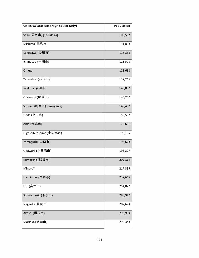
121
Cities w/ Stations (High Speed Only) Population
Saku (佐久市) [Sakudaira] 100,552
Mishima (三島市) 111,838
Kakegawa (掛川市) 116,363
Ichinoseki (一関市) 118,578
Ōmuta 123,638
Yatsushiro (八代市) 132,266
Iwakuni (岩国市) 143,857
Onomichi (尾道市) 145,202
Shūnan (周南市) [Tokuyama] 149,487
Ueda (上田市) 159,597
Anjō (安城市) 178,691
Higashihiroshima (東広島市) 190,135
Yamaguchi (山口市) 196,628
Odawara (小田原市) 198,327
Kumagaya (熊谷市) 203,180
Minato* 217,335
Hachinohe (八戸市) 237,615
Fuji (富士市) 254,027
Shimonoseki (下関市) 280,947
Nagaoka (長岡市) 282,674
Akashi (明石市) 290,959
Morioka (盛岡市) 298,348

122
Cities w/ Stations (High Speed Only) Population
Aomori (青森市) 299,520
Kurume (久留米市) 302,402
Takasaki (高崎市) 371,302
Toyohashi (豊橋市) 376,665
Nagano (長野市) 381,511
Gifu (岐阜市) 413,136
Fukuyama (福山市) 461,357
Kurashiki (倉敷市) 475,513
Himeji (姫路市) 536,270
Kagoshima (鹿児島市) 605,846
Okayama (岡山市) 709,584
Shizuoka (静岡市) 716,197
Kumamoto (熊本市) 734,474
Hamamatsu (浜松市) 800,866
Niigata (新潟市) 811,901
Kitakyūshū (北九州市) [Kokura] 976,846
Sendai (仙台市) 1,045,986
Hiroshima (広島市) 1,173,843
Saitama (さいたま市) 1,222,434
Kawasaki [Furukawa] 1,425,512
Fukuoka (福岡市) [Hakata] 1,463,743
Kyōto (京都市) 1,474,015

123
Cities w/ Stations (High Speed Only) Population
Kōbe (神戸市) 1,544,200
Nagoya (名古屋市) 2,263,894
Ōsaka (大阪市) 2,665,314
Yokohama (横浜市) 3,688,773
Tōkyō 8,945,695
Table 12 Summary of Coverage for Japan
Total Population residing in Cities/Towns with Stations 63,701,995
Total Population of Japan 127,450,460
% Population residing in Cities/Towns with Stations 49.98%
% Population Residing in City/Town with High Speed Stop 32.32%
Average Size of City/Town with High Speed Stop 441,707
Total Rail (km) (Climate Avenue, 2011) 13,000
(Brinkhoff, 2012)
Figure 22 Elevation Profile (left) and Population Density (right) for Spain with Rail Map
Table 13 Population of Cities/Towns in Spain with Stations

124
City Population Type of Track
Castillejo de Mesleón 158 Fast Speed
Canfranc 454 Non-Electrified
L'Alqueria d'Asnar 455 Non-Electrified
Fuentes de Oñoro 1,436 Non-Electrified
Ribes de Freser 2,001 Fast Speed
Pobla de Segur 3,237 Non-Electrified
Castejon 4,235 Fast Speed
Valencia de Alcántara 6,178 Non-Electrified
Puigcerdà 9,022 Fast Speed
Astorga 12,078 Non-Electrified
Zafra 16,424 Non-Electrified
Tui 17,262 Fast Speed
Manzanares 19,126 Non-Electrified
Monforte de Lemos 19,486 Fast Speed
Calatayud 20,837 High Speed
Riba-roja de Túria 21,094 Non-Electrified
Amposta 21,445 Fast Speed
Medina del Campo 21,607 High Speed
Cullera 23,304 Fast Speed
Olesa de Montserrat 23,924 Non-Electrified
Santa Perpètua de Mogoda 25,331 High Speed
Martorell 27,457 Fast Speed

125
Sant Vicenç dels Horts 28,137 Fast Speed
Sitges 28,617 Fast Speed
Mahon 29,125 Non-Electrified
Xàtiva 29,469 Non-Electrified
Redondela 30,006 Non-Electrified
Alcázar de San Juan 31,652 Fast Speed
Cambrils 33,008 Fast Speed
Aranda de Duero 33,229 Non-Electrified
Tortosa 34,432 Fast Speed
Águilas 34,990 Non-Electrified
Teruel 35,288
Vilagarcía (de Arousa) 37,903 Non-Electrified
Vilafranca (del Penedès) 38,785 Fast Speed
Miranda de Ebro 38,930 Fast Speed
Igualada 39,191
Soria 39,987 Non-Electrified
Vic 40,900 Fast Speed
Tres Cantos 41,065 Fast Speed
Plasencia 41,392 Non-Electrified
Alcantarilla 41,568 Non-Electrified
Antequera 41,854 Non-Electrified
Basauri 42,166 Fast Speed
Dénia 44,726 Non-Electrified

126
Figueres 44,765 Fast Speed
Colmenar Viejo 45,468 Fast Speed
Pinto 45,643 Fast Speed
Boadilla del Monte 46,151 Fast Speed
Santurtzi (Santurce-Antiguo) 47,076 Fast Speed
Eivissa (Ibiza) 49,388 Non-Electrified
Utrera 51,630 Fast Speed
Puertollano 52,200 High Speed
Mollet (del Vallès) 52,409 High Speed
Huesca 52,443 Non-Electrified
Segovia 55,220 High Speed
Aranjuez 55,755 Fast Speed
Cuenca 56,703
Mérida 57,797 Non-Electrified
Cerdanyola (del Vallès) 58,247 Fast Speed
Ávila 59,270 Fast Speed
Collado Villalba 60,998 Fast Speed
Irun (Irún) 61,006 Fast Speed
Alcoy (Alcoi) 61,093
Linares 61,110 Fast Speed
Castelldefels 63,139 Fast Speed
El Prat (de Llobregat) 63,499 Fast Speed
Zamora 65,525 Non-Electrified

127
Sagunto (Sagunt) 65,595 Fast Speed
Vilanova i la Geltrú 66,905 Fast Speed
Ponferrada 68,508 Fast Speed
Ferrol (El Ferrol) 72,963 Non-Electrified
Fuengirola 74,054 Fast Speed
Ciudad Real 74,798 High Speed
Manresa 76,589 Fast Speed
Gandía 78,704
San Sebastián de los Reyes 79,825 Fast Speed
Palencia 81,552 Fast Speed
Toledo 83,108 High Speed
Guadalajara 84,453
Talavera de la Reina 88,674 Non-Electrified
Las Rozas de Madrid 89,151 Fast Speed
Lorca 92,869 Non-Electrified
Cáceres 95,026 Non-Electrified
Santiago de Compostela 95,207 Non-Electrified
Girona (Gerona) 96,722 Fast Speed
San Fernando 96,894 Fast Speed
Lugo 98,007 Non-Electrified
Reus 106,709 Fast Speed
Ourense (Orense) 108,002 Non-Electrified
Jaén 116,781 Fast Speed
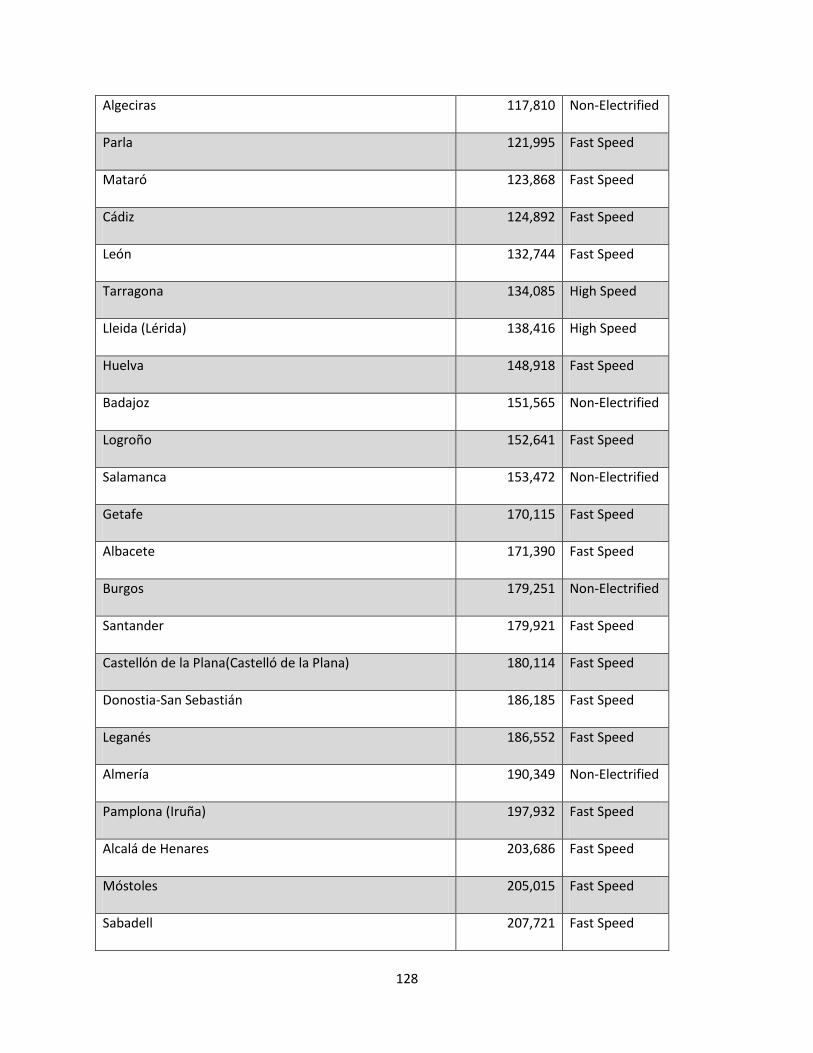
128
Algeciras 117,810 Non-Electrified
Parla 121,995 Fast Speed
Mataró 123,868 Fast Speed
Cádiz 124,892 Fast Speed
León 132,744 Fast Speed
Tarragona 134,085 High Speed
Lleida (Lérida) 138,416 High Speed
Huelva 148,918 Fast Speed
Badajoz 151,565 Non-Electrified
Logroño 152,641 Fast Speed
Salamanca 153,472 Non-Electrified
Getafe 170,115 Fast Speed
Albacete 171,390 Fast Speed
Burgos 179,251 Non-Electrified
Santander 179,921 Fast Speed
Castellón de la Plana(Castelló de la Plana) 180,114 Fast Speed
Donostia-San Sebastián 186,185 Fast Speed
Leganés 186,552 Fast Speed
Almería 190,349 Non-Electrified
Pamplona (Iruña) 197,932 Fast Speed
Alcalá de Henares 203,686 Fast Speed
Móstoles 205,015 Fast Speed
Sabadell 207,721 Fast Speed

129
Jerez de la Frontera 210,861 Fast Speed
Terrassa (Tarrasa) 213,697 Fast Speed
Cartagena 214,918 Non-Electrified
Oviedo 225,391 Fast Speed
Elche (Elx) 230,354 Non-Electrified
Vitoria-Gasteiz 239,562 Fast Speed
Granada 240,099 Non-Electrified
A Coruña (La Coruña) 246,028 Non-Electrified
Gijón 277,559 Fast Speed
Vigo 297,241 Fast Speed
Valladolid 313,437 High Speed
Córdoba 328,659 High Speed
Alicante (Alacant) 334,329 Fast Speed
Bilbao 352,700 Fast Speed
Palma de Mallorca 405,318 Non-Electrified
Murcia 442,203 Non-Electrified
Málaga 568,030 High Speed
Zaragoza 674,725 High Speed
Sevilla 703,021 Fast Speed
Valencia (València) 798,033 High Speed
Barcelona 1,615,448 High Speed
Madrid 3,265,038 High Speed

130
Table 14 Summary of Coverage for Spain
Total Population of Cities/Towns with Stations 20,345,890
Total Population 46,081,574
% Population Located within Cities/Towns with Stations 44.15%
Total Rail (km) 15,288
(Brinkhoff, 2012)
Figure 23 Elevation Profile (left) and Population Density (right) for Switzerland with Rail Map
Table 15 Population of Cities/Towns in Switzerland with Stations
Station-Cities Pop 12-31-2010
Rail
speed(s)
Wasserauen 30 High
Ziegelbrücke 70 High
Montbovon 265 High
Tiefencastel 269 High
Göschenen 410 High
Wassen 434 High
Filisur 461 High

131
Buttes 601 High
Les Verrières 667 High
Sembrancher 862 High
St. Gingolph 888 High
L'Isle 975 High
Linthal 1,088 High
Les Brenets 1,089 High/Non-Ev
Bercher 1,109 High
Zemez 1,140 High
Tamins 1,184 High
Glovelier 1,204 High
Waldenburg 1,221 High
Kandersteg 1,231 High
Les Ponts-de-Martel 1,265 High
Champéry 1,276 High
Andermatt 1,304 High
Rodersdorf 1,315 High
Palézieux 1,326 High
Boltigen 1,376 High
Ormont-Dessus 1,457 High
Bière 1,480 High
Airolo 1,558 High
Le Noirmont 1,661 High

132
Trogen 1,687 High
Fahrwangen 1,862 High
Flüelen 1,950 High
Pontresina 1,994 High
Disentis 2,111 High
St. Sulpice 2,123 High
Arosa 2,251 High
Broc 2,296 High
Ilanz 2,315 High
Scuol 2,376 High
Lenk im Simmertal 2,399 High
Muhlenberg 2,654 High
Niederweningen 2,729 High
Thusis 2,791 High
Zweisimmen 2,922 High
Samedan 2,968 High
Brienz 2,981 High
Gais 3,065 High
Orsières 3,077 High
Gstaad 3,200 High
Stein am Rhein 3,209 High
Ins 3,229 High
Vallorbe 3,312 High

133
Nesslau 3,348 High
Cossonay 3,368 High
Leuk 3,381 High
Tavannes 3,478 High
Poschiavo 3,506 High
Fleurier 3,518 High
Schöftland 3,715 High
Leysin 3,839 High
Klosters 3,892 High
Engelberg 3,903 High
Heiden 3,990 High
St. Moritz 4,202 High
Eglisau 4,213 High
Le Chenit 4,325 High
St. Croix 4,509 High
Meiringen 4,583 High
Romont 4,588 High
Kerzers 4,598 High
Huttwil 4,704 High
Konolfingen 4,763 High
St. Imiier 4,771 High
Sumiswald 5,027 High
Echallens 5,189 High

134
Oensingen 5,245 High
Flamat 5,322 High
Sargans 5,330 High
Interlaken 5,429 High
Estavayer 5,554 High
Alpnach 5,568 High
St. Margrethen 5,568 High
Appenzell 5,712 High
Zermatt 5,720 High
Châtel-Saint-Denis 5,727 High
Balsthial 5811 High
Uznach 5,840 High
Glarus 5,877 High
Murton 6,125 High
Sissach 6,275 High
Bex 6,500 High
Porrentruy 6,679 High
Schwarzenburg 6,716 High
Frutigen 6,718 High
Herzogenbuchsee 6,766 High
Visp 7,014 High
Moutier 7,466 High
Bagnes 7,726 High

135
Chiasso 7,737 High
Stans 7,961 High
Egg 7,997 High
Aigle 8,100 High
Wattwil 8,130 High
Lenzburg 8,341 High
Ingenbohl 8,411 High
Payerne 8,728 High
Altdorf 8,861 High
Sursee 8,941 High
Langnau 9,017 High
Rotkreuz 9,085 High
Romanshorn 9,606 High
Suhr 9,743 High
Sarnen 9,971 High
Le Locle 10,049 High
Weinfelden 10,383 High
Brugg 10,386 High
Arth (-Goldau) 10,699 High
Zofingen 10,803 High
Val-de-Travers 10,812 High
Altstätten 10,819 High
Davos 11,166 High

136
Buchs 11,242 High
Villars-sur-Glâne 11,397 High
Delémont 11,639 High
Lyss 11,821 High
Brig-Glis 12,467 High
Spiez 12,475 High
Muri bei Bern 12,625 High
Küsnacht 13,501 High
Liestal 13,600 High
Einsiedeln 14,385 High
Schwyz 14,423 High
Wohlen 14,443 High
Morges 14,744 High
Langenthal 14,938 High
Locarno 15,153 High
Herisau 15,236 High
Burgdorf 15,374 High
Steffisburg 15,431 High
Sierre 15,527 High
Illnau-Effretikon 15,602 High
Grenchen 15,928 High
Solothurn 16,066 High
Martigny 16,143 High

137
Monthey 16,408 High
Olten 16,987 High
Thalwil 17,213 High
Bellinzona 17,373 High
Bülach 17,511 High
Gossau 17,763 High
Baden 17,929 High
Wil 18,000 High
Vevey 18,394 High
Reinach 18,656 High
Nyon 18,728 High
Bulle 18,947 High
Aarau 19,497 High
Kreuzlingen 19,544 High
Wädenswil 20,433 High
Wetzikon 22,118 High
Frauenfeld 23,298 High
Dietikon 23,624 High
Landquart 24,093 High
Montreux 24,579 High
Rapperswil-Jona 26,212 High
Zug 26,327 High
Yverdon-les-Bains 27,511 High

138
Sion 30,363 High
Uster 32,265 High
Neuchâtel 33,054 High
Chur 33,756 High
Fribourg 34,897 High
Schaffhausen 34,943 High/Non-Ev
La Chaux-de-Fonds 37,504 High
Thun 42,623 High
Biel (Bienne) 51,203 High
Lugano 54,667 High
St. Gallen 72,959 High
Luzern 77,491 High
Winterthur 101,308 High
Bern 124,381 High
Lausanne 127,821 High
Basel 163,216 High
Genève [Geneva] 187,470 High/Basic
Zürich [Zurich] 372,857 High
Table 16 Summary of Coverage for Switzerland
Total Population of Cities/Towns with Stations 2,948,644
Total Population 7,825,243
% Population Located within Cities/Towns with Stations 37.68%

139
Total Rail (km) 5,063
(Brinkhoff, 2012)
Figure 24 Elevation Profile (left) and Population Density (right) for the US with Rail Map
Table 17 Population of Cities/Towns in the US with Amtrak Stations
Station City Population of City (Mid 2009) Type of Rail
Thurmond 7 Basic
Prince 116 Basic
Wishram 339 Basic
Bingen 678 Basic
Yemassee 867 Basic
Alderson 1,064 Basic
Pittsfield 1,334 Basic
Colfax 1,878 Basic
Montgomery 1,912 Basic
New Iberia 2,086 Basic
Martinsburg 2,137 Basic
White Sulphur Springs 2,263 Basic
Hinton 2,533 Basic
Dover 2,682 Basic
Denmark 2,934 Basic
Kingstree 3,176 Basic
Rutland 3,250 Basic
Surf (Lompoc) 3,338 Basic
Denair 3,880 High Speed
Clifton Forge 3,927 Basic
Hazlehurst 4,327 Basic
Walnut Ridge 4,720 Basic
McGrego 4,910 Basic
Mineola 5,219 Basic

140
Hamlet 5,764 Basic
Pauls Valley 6,067 Basic
Schriever 6,114 Basic
Purcell 6,224 Basic
Guadalupe 6,594 Basic
Camden 7,103 Basic
St. Albans 7,243 Basic
Bay St. Louis 7,538 Basic
Rensselaer 7,851 Basic
Malvern 8,854 Basic
Toccoa 9,065 Basic
Louisville 9,453 High Speed
Summit 10,169 Basic
Brookhaven 10,207 Basic
Palatka 10,677 Basic
Fort Madison 10,884 Basic
Arkadelphia 11,175 Basic
Niles 11,272 Basic
Picayune 12,008 Basic
Elizabethtown 12,103 Basic
Kelso 12,150 Basic
Kewanee 12,241 Basic
Rantoul 12,247 Basic
Effingham 12,557 Basic
New Carrollton 12,656 Basic
Williamsburg 12,729 Basic
Southern Pines 12,862 Basic
Claremont 12,963 Basic
Clemson 13,002 Basic
Solana Beach 13,059 High Speed
Grover Beach 13,200 Basic
Auburn 13,352 Basic
Centralia 13,465 Basic
McComb 13,644 Basic
Carpinteria 13,764 Basic
Aberdeen 14,099 Basic
Lincoln 14,523 Basic
Yazoo City 14,798 Basic
Crawfordsville 15,090 Basic
La Grange 15,186 Basic
Greensburg 15,255 Basic

141
Depew 15,261 Basic
Red Wing 15,681 Basic
Centralia 15,700 Basic
Greenwood 15,808 Basic
Dyer 15,927 Basic
Truckee 16,260 Basic
Corcoran 16,446 High Speed
Mattoon 17,120 Basic
Tukwila 17,392 Basic
Amsterdam 17,465 Basic
Saco 18,204 Basic
Laurel 18,831 Basic
Warrensburg 19,203 Basic
Plattsburgh 19,380 High Speed
Macomb 19,748 Basic
Hammond 20,037 Basic
Carbondale 20,196 Basic
Texarkana 20,221 Basic
Cumberland 20,449 Basic
Sedalia 21,151 Basic
Johnstown 21,497 Basic
Alliance 22,586 Basic
Fredricksburg 23,193 Basic
Anniston 23,589 Basic
Pascagona 23,677 Basic
Marshall 24,089 Basic
Barstow 24,528 Basic
Wasco 24,724 High Speed
Ardmore 24,850 Basic
New London 26,184 Basic
Winona 26,502 Basic
Kirkwood 26,808 Basic
Kankakee 26,840 Basic
Suisun 27,003 Basic
Slidell 27,475 Basic
Salisbury 27,808 Basic
Winter Park 28,449 Basic
Saratoga Springs 29,126 Basic
Alton 29,264 Basic
Poughkeepsie 29,564 Basic
Cleburne 29,931 Basic

142
Port Huron 30,568 Basic
Galesburg 31,006 Basic
Oregon City 31,826 Basic
Mount Vernon 32,139 Basic
Florence 32,180 Basic
Chatsworth 32,188 Basic
Petersburg 32,986 Basic
Jackson 33,315 Basic
Rome 33,443 Basic
Holland 34,053 Basic
San Juan Capistrano 35,142 Basic
Gainesville 35,750 Basic
Manassas 36,514 Basic
Del Rio 36,676 Basic
Moorpark 36,695 Basic
Woburn 38,987 Basic
Meridian 39,695 Basic
Quincy 40,062 Basic
Spartanburg 40,387 Basic
Edmonds 40,773 Basic
Jefferson City 41,297 Basic
Lacey 42,046 Basic
Paso Robles 42,751 Basic
Kannapolis 43,404 Basic
San Luis Obispo 44,075 Basic
Danville 44,400 Basic
East Lansing 45,563 Basic
Biloxi 45,768 Basic
Glenview 46,207 Basic
Altoona 46,287 Basic
Harrisburg 47,418 Basic
Palm Springs 48,181 Basic
Albany 48,582 Basic
Wilson 48,721 Basic
Huntington 49,129 Basic
Hanford 50,053 High Speed
La Crosse 50,980 Basic
Sanford 50,998 Basic
Niagara Falls 51,295 Basic
Burlington 51,577 Basic
New Brunswich 51,579 Basic

143
Normal 52,799 Basic
Elkhart 53,060 Basic
San Marcos 53,205 Basic
Hattiesburg 53,533 Basic
Rocklin 53,572 Basic
Elyria 54,969 Basic
Goleta 55,302 Basic
Lancaster 55,439 Basic
Madera 56,692 Basic
Utica 58,040 Basic
Meriden 59,186 Basic
Taylor 59,308 Basic
Rocky Mount 59,576 Basic
Temple 60,118 Basic
Lodi 61,450 High Speed
Schenectady 61,469 Basic
Haverhill 61,588 Basic
San Clemente 61,610 Basic
Greenville 61,782 Basic
Rockville 62,105 Basic
Kissimmee 62,632 Basic
Davis 62,947 Basic
Portland 63,008 Basic
Delray Beach 64,691 High Speed
Lafayette 65,704 Basic
Pontiac 66,247 Basic
St. Cloud 67,136 Basic
Deerfield Beach 69,144 High Speed
Gulfport 70,732 Basic
Lake Charles 71,475 Basic
Kalamazoo 72,825 Basic
Gastonia 72,934 Basic
Lynchburg 73,933 Basic
New Rochelle 74,323 Basic
Merced 76,273 High Speed
Hammond 76,545 Basic
Longview 78,038 Basic
Bellingham 80,055 Basic
Champaign 80,286 Basic
Trenton 83,242 Basic
Dearborn 84,575 Basic

144
Santa Barbara 86,353 Basic
Lees Summit 86,556 Basic
Sparks 89,346 Basic
Wilmington 89,621 Basic
Tuscaloosa 93,215 Basic
Lakeland 93,738 Basic
North Charleston 97,601 Basic
Everett 99,384 Basic
West Palm Beach 99,504 High Speed
Antioch 101,182 Basic
Berkeley 102,822 Basic
Burbank 103,121 High Speed
High Point 103,396 Basic
Erie 103,571 Basic
South Bend 104,215 Basic
Gainsville 104,875 Basic
Norman 109,063 Basic
Beaumont 110,099 Basic
Ventura 110,873 Basic
Victorville 110,873 Basic
Flint 111,475 Basic
Santa Clara 111,997 Basic
Ann Arbor 112,852 Basic
Lafayette 114,915 Basic
Roseville 115,687 Basic
Springfield 118,033 Basic
Stamford 121,026 Basic
Fayetteville 123,287 Basic
New Haven 123,330 Basic
Hartford 124,060 Basic
Columbia (SC) 129,333 Basic
Fullerton 132,620 High Speed
Cary 136,600 Basic
Bridgeport 137,298 Basic
Syracuse 138,560 Basic
Hollywood 142,622 High Speed
Salinas 144,276 Basic
Hayward 144,289 Basic
Joliet 147,633 Basic
Pomona 152,367 High Speed
Eugene 153,231 Basic

145
Salem 155,719 Basic
Fort Lauderdale 163,160 High Speed
Vancouver 165,809 High Speed
Van Nuys 166,616 Basic
Santa Clarita 169,174 High Speed
Ontario 171,602 High Speed
Providence 171,909 Basic
Tallahassee 172,574 Basic
Oceanside 172,901 Basic
Jackson 175,021 Basic
Worcester 182,421 Basic
Oxnard 187,535 Basic
Little Rock 191,930 Basic
Mobile 193,171 Basic
Grand Rapids 193,710 Basic
Glendale 196,847 High Speed
San Bernardino 198,410 High Speed
Tacoma 199,637 Basic
Yonkers 201,162 Basic
Modesto 202,747 High Speed
Richmond 204,451 Basic
Fremont 205,514 Basic
Rochester 207,294 Basic
Irvine 209,716 High Speed
Reno 219,636 Basic
Durham 229,174 Basic
Birmingham 230,131 High Speed
Orlando 235,860 High Speed
Greensboro 255,061 Basic
Buffalo 270,240 High Speed
Newark 278,154 Basic
Stockton 287,578 High Speed
Riverside 297,859 High Speed
Pittsburgh 311,647 Basic
Toledo 316,238 High Speed
Bakersfield 324,463 High Speed
Cincinnati 333,013 High Speed
Santa Ana 340,340 High Speed
Tampa 343,890 High Speed
New Orleans 354,850 Basic
St. Louis 356,587 High Speed

146
Wichita 382,368 High Speed
Minneapolis 385,542 High Speed
Tulsa 389,625 High Speed
Raleigh 405,791 High Speed
Oakland 409,184 Basic
Colorado Springs 416,427 High Speed
Cleveland 431,363 High Speed
Miami 433,136 High Speed
Sacramento 466,687 High Speed
Fresno 479,921 High Speed
Kansas City 482,299 High Speed
Atlanta 540,921 High Speed
Albuquerque 545,852 High Speed
Oklahoma City 560,332 High Speed
Portland 566,141 High Speed
Las Vegas 567,641 High Speed
Denver 600,158 High Speed
Washington 601,723 High Speed
Milwaukee 604,133 High Speed
Seattle 617,334 High Speed
Baltimore 637,418 High Speed
Boston 645,169 High Speed
Charlotte 709,441 High Speed
Fort Worth 727,575 Basic
Columbus 769,360 High Speed
Austin 786,382 High Speed
Indianapolis 807,584 High Speed
Jacksonville 813,518 High Speed
San Francisco 815,358 High Speed
Detroit 910,920 High Speed
San Jose 964,695 High Speed
Dallas 1,299,543 High Speed
San Diego 1,306,301 High Speed
San Antonio 1,373,668 High Speed
Philadelphia 1,547,297 High Speed
Houston 2,257,926 High Speed
Chicago 2,851,268 High Speed
Los Angeles 3,831,868 High Speed
New York City 8,391,881 High Speed
Disclaimers

147
Amtrak stations only Bold cities are proposed high speed stations
Table 18 Summary of Coverage for the US
Population With Station in City 58,773,423
Total Population 307,006,550
% Population in city of station 19.14%
Total Rail (km)* 21,200
*only current length of Amtrak, does not take into account of proposed tracks (National Railroad
Passenger Corporation, 2012)
(Brinkhoff, 2012)
H.1.2. Cost
Table 19 Cost of Building Rails/km from International Rails
Country Rail Type
Cost/km
(in
millions) Currency Year Source Comments
Belgium
High
Speed 15 US $ 2005 (Arduin & Ni, 2005)
California
High
Speed 14 US $ 1994
(Levinson, Mathieu, Gillen, &
Kanafani, 1997)
Proposal/estimates (details found
on the 'California Estimates' Tab)
China
Main
Line 9.1 US $ 2011
(Net Resources International,
2011)
Tyichang-Wanzhou line (377 km),
Surface with 278km in tunnel or
bridges
China
High
Speed 10 US $ 2010
(Net Resources International,
2011) Haikou-Sanya Line (308 km)
Denmark
Metro
Line 247.5 US $
2011-
2018
(Net Resources International,
2011)
Copenhagen (16 km), all
underground

148
Country Rail Type
Cost/km
(in
millions) Currency Year Source Comments
England Upgrades 69 pounds 2011
(Net Resources International,
2011)
Crossrail, London; New twin bore
tunnels
France
High
Speed 10 US $ 2005 (Arduin & Ni, 2005)
France
High
Speed 3.4 US $ 1994
(Levinson, Mathieu, Gillen, &
Kanafani, 1997)
TGV average (details found on
'French TGV' tab)
France Upgrades 35 Euros 2010
(Net Resources International,
2011) RFF, new double-track line
Germany
High
Speed 15 US $ 2005 (Arduin & Ni, 2005)
Germany
High
Speed 57 Euros 2010
Infrastructure Cost Review:
Technical Report
Germany
High
Speed 44.4 US $ 2008
(Net Resources International,
2011)
Germany
High
Speed 89 US $ 2010
(Net Resources International,
2011) Nuremburg-Munich
Germany
High
Speed 60 US $ 2010
(Net Resources International,
2011) Stuttgart 21
Germany
High
Speed 171 US $ 2010 (Smith, 2009) Nürnberg-Ingolstadt-München
Italy
High
Speed 25 US $ 2005 (Arduin & Ni, 2005)
Korea
High
Speed 35 US $ 2005 (Arduin & Ni, 2005)
Korea
Airport
Line 98.1 US $ 2010
(Net Resources International,
2011) Seoul-Gimpo Line (20.4 km)

149
Country Rail Type
Cost/km
(in
millions) Currency Year Source Comments
Netherlands
High
Speed 53 US $ 2005 (Arduin & Ni, 2005)
Spain
High
Speed 10 US $ 2005 (Arduin & Ni, 2005)
Spain
High
Speed 9.57 Euros 2010
(Net Resources International,
2011) Madrid-Albacete line (304 kms)
Spain Upgrades 2.125 Euros 2011
(Net Resources International,
2011) Route Doubling and electrification
Spain
High
Speed 60.5 Euro 2010 (Live, 2010) Pajares de Vienteres; 3006 M€ por
49.7 km
Spain
High
Speed 35.7 Euro 2008 (Live, 2010)
Ourense-Pontevedra/Vigo-Cerdedo
AV
Spain
High
Speed 21.72 Euro 2006 (Live, 2010) Madrid-Segovia-Valladolid
Spain
High
Speed 22.57 Euro
(Live, 2010) Basque; under construction
Spain
High
Speed 19.24 Euro
(Live, 2010) Cordoba-Malaga
Spain
High
Speed 15.88 Euro
(Live, 2010)
Madrid-Zaragoza-Barcelona French
Border
Spain
High
Speed 15.07 Euro 2010 (Live, 2010)
Madrid-Levante; 6600M€ for
438km
Spain
High
Speed 4.88 Euro 2001 (Live, 2010) Madrid Sevilla
Switzerland
High
Speed 33.1 CHF 2010 (Net Resources International, 2011)

150
Country Rail Type
Cost/km
(in
millions) Currency Year Source Comments
Switzerland Upgrades 109 Euros
2011-
2016
(Net Resources International,
2011) Bremmer; New twin born tunnels
Switzerland
High
Speed 32.288 CHF 2010 (SBB CFF FFS) Mattstetten–Rothrist New Line
Switzerland
High
Speed 94.5 CHF 2010 (SBB CFF FFS) Zimmerberg Base Tunnel
Switzerland
High
Speed 73 CHF 2010 (SBB CFF FFS) Adler Tunnel
Switzerland
High
Speed 35.5 CHF 2010 (SBB CFF FFS) Vauderens Tunnel
Switzerland
High
Speed 47 CHF 2010 (SBB CFF FFS) NRLA
Switzerland
High
Speed 165 CHF 2010
(Net Resources International,
2011) AlpTransit Gotthard
Switzerland
High
Speed 145 CHF 2010
(Net Resources International,
2011) Ceneri Tunnel
Switzerland
High
Speed 6.5 CHF 2010
(Net Resources International,
2011)
Rhine, Switzerland to Rhone,
France
Taiwan
High
Speed 37 US $ 2005 (Arduin & Ni, 2005)
UK
High
Speed 74 US $ 2005 (Arduin & Ni, 2005)

151
Figure 25 Average Unit Cost for international rails
H.1.3. Frequency and Travel Times
Figure 26 Travel Times for France TGV
(Arduin & Ni, 2005)
Table 20 Travel Times and Frequencies for German Rails
High-Speed

152
InterCity Express
Hours of Operation: 24 hours
Frequency: 1-2 hours
Berlin-Frankfurt
4.1
hours
Berlin-Hamburg
1.6
hours
Berlin-Munich
5.8
hours
Frankfurt-Munich
3.2
hours
Nuremburg-Vienna
4.9
hours
InterCity
Hours of Operation: 24 hours
Frequency: 1-2 hours
Berlin-Munich
5.8
hours
Frankfurt-Munich
3.2
hours
Berlin-Frankfurt
4.1
hours
Frankfurt-Cologne
1.2
hours
Frankfurt-Stuttgart
1.3
hours

153
EuroCity
Hours of Operation: 24 hours
Frequency: 1-2 hours
Fast-Speed
InterCityNight
Hours of Operation : Overnight (6PM to noon)
Frequency: Once (per destination)
EuroNight
Hours of Operation : Overnight (6PM to noon)
Frequency: Once (per destination)
CityNightLine
Hours of Operation : Overnight (6PM to noon)
Frequency: Once (per destination)
Nachtzug
Hours of Operation : Overnight (6PM to noon)
Frequency: Once (per destination)
RegionalExpress
Hours of Operation: 24 hours
Frequency: 30-120 min

154
StadtBahn
Hours of Operation: 24 hours
Frequency: 10-20 min
S-Bahn
Hours of Operation: 24 hours
Frequency: 20-30 min
U-Bahn
Hours of Operation: 24 hours
Frequency: 5-15 min
(Purcell, 2010)
(Rail Europe, Inc., 2012)
Table 21 Travel Time and Frequency of Rail in Great Britain
Operate from 6:00 til 0:00
Fast Speed
Travel Time Sources
London Blackfriars to Glasgow
5.5 hrs* (run every 30
mins)
(Association of Train Operating
Companies)
London Euston to Glasgow 5 hrs* (run every hour)
(Association of Train Operating
Companies)
London Euston to Liverpool
2 hrs* (run twice every
half hour)
(Association of Train Operating
Companies)
* Some trains do not run
direct; these trains take
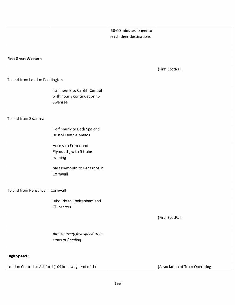
155
30-60 minutes longer to
reach their destinations
First Great Western
(First ScotRail)
To and from London Paddington
Half hourly to Cardiff Central
with hourly continuation to
Swansea
To and from Swansea
Half hourly to Bath Spa and
Bristol Temple Meads
Hourly to Exeter and
Plymouth, with 5 trains
running
past Plymouth to Penzance in
Cornwall
To and from Penzance in Cornwall
Bihourly to Cheltenham and
Gluocester
(First ScotRail)
Almost every fast speed train
stops at Reading
High Speed 1
London Central to Ashford (109 km away; end of the
(Association of Train Operating

156
line) Companies)
37 minute train ride
(HS1)
Trains leave once per hour
(Rail Saver)
Table 22 Travel Times and Frequencies for Italian Rail
Operate from roughly
5:30 til 0:00
Trains
Travel Times Additional Comments Sources
High Speed
Frecciarossa
"High Speed Line" - Reach
speeds of up to 360 km/h (Gruppo Ferrovie, 2008)
Milan-Rome-Milan
68 daily
connections
3 hrs-no stop (roughly
every hour)
(International Rail
Australasia )
3.5 hrs-stop at Bologna
and Florence (roughly
every hour)
2.75 hrs-stop in Milan
Rogoredo (4 throughout
the day)
Milan-Naples-Milan
37 daily
connections
4.5 hrs-stop at Milan
Rogoredo ( 4 throughout
the day)
4.5 hrs-stop at Rome (7
throughout the day)
5 hrs-stop at Bologna,

157
Florence, and Rome
(Once every hour)
Turin-Rome-Turin
14 daily
connections
4.5 hrs-stop in Milan,
Bologna, and Florence
(roughly every hour)
4.33 hrs-stop at Milan (4
throughout the day)
Bologna-Florence-
Bologna
46 daily
connections
Rome-Naples-Rome
40 daily
connections 1.17 hrs
Eurostar Italia
"High Speed Line" that
connects the European
countries (Gruppo Ferrovie, 2008)
Connect Rome to
Ancona, Genoa,
~3 hrs (run roughly every
2 hrs) from Ancona to
Roma
(International Rail
Australasia )
Lamezia Terme, Reggio
Calabria,
Perugia, Ravenna, Rimini, and Taranto
~6-6.5 hrs (run roughly
every hour) from Taranto
to Roma
Fast Speed
Frecciargento
"Fast Speed Line" Reach
speeds of up to 250 km/h (Gruppo Ferrovie, 2008)
Rome-Venice-Rome
26 daily
connections 3.5 hrs (2 every day)
3.75 hrs (every half hour)
Rome-Verona-Rome
6 daily
connections 3 hrs

158
Rome-Bari-Rome
8 daily
connections 4 hrs (once a day)
6 hrs (the non-fast trains)
Rome-ReggioCalabria-
Rome
2 daily
connections 4 hrs
Basic Speed
Frecciabiance
Stop at all stations along
the lines
Reach speeds of up to 200
km/h (Gruppo Ferrovie, 2008)
Connect Milan to: Venice, Udine e
Trieste,
Run regularly throughout
the day (hourly)
(International Rail
Australasia )
Genoa e Rome, down to Bari, Lecce
Table 23 Travel Times and Frequency of Japanese Rail
High Speed Trains (Bullet Trains)
Tokaido
Shinkansen
Trains reach speeds of up to 270 km/h
Connects Japan's 3 largest metropolitan areas
Departures every few minutes
Nozomi
2.5 hours from Tokyo to Shin-Osaka
Departs 4 times per hour (more often during peak hours)
Most continue along Sanyo Shinkansen to Hiroshima or Hakata
Most cars are reserved seating; however, there 2-3 non-reserved cars per train

159
Hikari
3 hrs from Tokyo to Shin-Osaka
Departs 2 times per hour
Slightly more non-reserved seating, but still most reserved seating cars
Kodama
4 hrs from Tokyo to Shin-Osaka
Departs 2 times per hour
Some trains during rush hour are fully non-reserved
Sanyo Shinkansen
Trains reach speeds of up to 300 km/h
Nozomi
2.5 hrs from Shin-Osaka to Hakata
Departs 3 times per hour (2 to/from Hakata, 1 to/from Hiroshima)
More service provided during peak hours
8-car Hikari
Railstar
Slightly slower than the Nozomi
16-car Hikari
Runs each hour
Stops at every station between Shin-Osaka and Okayama

160
Kodama
5 hrs from Shin-Osaka to Hakata
Stops at every station
Mizuho
Faster than Nizomi
Provides through service to Kyushu Shinkansen to/from Kangoshima
4 round trips per day in am and pm
Sakura
Similar to Mizuho but stops at more stations
Tohoku
Shinkansen
Hayabusa
Fastest train category on line
Serves Tokyo, Omiya, Sendai, Morioka, and Shin-Aomori Stations only
2 round trips per day
# of services to be increased in the future
Runs up to 300 km/h
Planned to be increased to 320 km/h in 2013
No non-reserved seating
Hayate
Second fastest train on line

161
Runs same route as Hayabusa, but with more stops
No non-reserved seating
Yamabiko
Third fastest category
Runs to Morioka, though some stop at Sendai
Some trains are 2 story, called MAX Yamabiko
Nasuno
Slowest train category
Serves all stations between Tokyo and Koriyama
Komachi
Only train category of the Akita Shinkansen
Couled with a Hayate train between Tokyo and Morioka
Run on their own between Morioka and Akita
No reserved seating
Tsubasa
Only train category of the Yanmagata Shinkansen
Almost all trains are coupled with a MAX Yamabiko between Tokyo and
Fukushima
Run on their own between Fukushima and Shinjo
Some trains stop at Yanmagata Station
Joetsu Shinkansen

162
Toki
Faster of the 2 train categories
Runs between Tokyo and Niigata stations
Some use 2 story trains, called MAX Toki
Tanigawa
Slower of the 2 train categories
Serves all stations between Tokyo and Echigo-Yuzawa stations
During the winter, some trains continue to Gala Yuzawa Station
Base of the Gala Yuzawa ski resort
Nagano Shinkansen
Scheduled to be extended to Kanzawa by 2015
Asama
Operates between Tokyo and Nagano stations
Different stopping patterns
Kyushu Shinkansen
Planned Nagaski branch line
Mizuho
Fastest train category
Stops at Hakata, Kumamoto, and Kagoshima-Chuo only
Through service to Sanyo Shinkansen to and from Shin-Osaka
4 round trips per day in am and pm

163
Sakura
Second fastest train category
Serves more stations than Mizuho
1 or 2 departures per hour
Some trains providing through service to/from Shin-Osaka
Tsubane
Slowest train category
Stops at all stations
Most trains run between Hakata and Kumamoto only
(Japan-Guide.com, 2012)
Table 24 Travel Times and Frequency of Spanish Rails
High Speed
AVE
Madrid to Barcelona
Average duration
169 min based off of 25 trains
2hr49min
Hours of Operation
5:50
22:50

164
Frequency of Deperature
36.4 min
average deperature of each train
AVE
Madrid to Sevilla
Average duration
151min
2hr31min
Frequency of Departure based on 19 trains
45.25min
Average
AVE
Madrid to Valladolid
Average Duration
56min
Frequency of Deperature 2 trains
7hr50min
AVE
Madrid to Huesca

165
Duration
133
Frequency of Deperature 1 train
19:05
AVE
Madrid to Malaga
Average Duration
155.23min
Frequency of Deperature 10 Trains
84min
AVE
Barcelona to Sevilla
Average Duration
150.5min
Average Frequency of Deprature 17
53.23mi
AVE
Barcelona to Malaga
Average Duration

166
350
Average Frequency of Deperatures 2 trains
350min
(Passengers - Timetables)
Table 25 Travel Times and Frequency of Swiss Rails
High-Speed
Zürich Verkehrsverbund
Hours of Operation: 24 hours
Frequency: 30-60 min
Zurich-Bern
1.1
hours
Zurich-Lausanne
2.2
hours
Zurich-Geneva
2.8
hours
Zurich-
Winterthur
0.4
hours
Zurich-Luzern
0.9
hours
Tarifverbund Nordwestschweiz
Hours of Operation: 24 hours
Frequency: 30-60 min
Basel-Zurich
1.2
hours
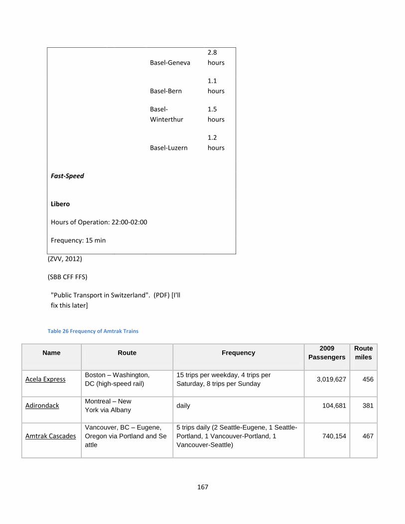
167
Basel-Geneva
2.8
hours
Basel-Bern
1.1
hours
Basel-
Winterthur
1.5
hours
Basel-Luzern
1.2
hours
Fast-Speed
Libero
Hours of Operation: 22:00-02:00
Frequency: 15 min
(ZVV, 2012)
(SBB CFF FFS)
"Public Transport in Switzerland". (PDF) [I'll
fix this later]
Table 26 Frequency of Amtrak Trains
Name Route Frequency 2009
Passengers
Route
miles
Acela Express Boston – Washington,
DC (high-speed rail)
15 trips per weekday, 4 trips per
Saturday, 8 trips per Sunday 3,019,627 456
Adirondack Montreal – New
York via Albany daily 104,681 381
Amtrak Cascades Vancouver, BC – Eugene,
Oregon via Portland and Se
attle
5 trips daily (2 Seattle-Eugene, 1 Seattle-
Portland, 1 Vancouver-Portland, 1
Vancouver-Seattle)
740,154 467

168
Name Route Frequency 2009
Passengers
Route
miles
Auto Train Lorton, Virginia – Sanford,
Florida daily 232,955 855
Blue Water Chicago – Port Huron,
Michigan daily 132,851 319
California Zephyr Chicago – Emeryville,
California(Oakland/San
Francisco)
daily 345,558 2,438
Capitol Corridor Auburn, California –
Sacramento– San
Jose via Oakland
16 trips per weekday (8 Oakland-
Sacramento, 7 San Jose-Sacramento, 1
Oakland-Auburn), 11 trips per
Saturday/Sunday (6 San Jose-
Sacramento, 4 Oakland-Sacramento, 1
San Jose-Auburn)
1,599,625 172
Capitol Limited Chicago – Washington,
DC viaCleveland and Pittsbu
rgh
daily 215,371 764
Cardinal Chicago – New
York viaIndianapolis, Cincin
nati, andWashington, DC
3 trips per week 108,614 1,147
Carl Sandburg Chicago – Quincy, Illinois daily 202,558 258
Carolinian New York – Charlotte, North
Carolina daily 277,740 704
City of New
Orleans Chicago – New Orleans daily 196,659 926
Coast Starlight Seattle – Los
Angeles viaSacramento and
Oakland
daily 432,565 1,377
Crescent New York – New
Orleans viaAtlanta daily 286,576 1,377
Downeaster Portland, Maine – Boston 5 trips daily 460,474 116

169
Name Route Frequency 2009
Passengers
Route
miles
Empire Builder Chicago – Portland,
Oregon/Seattle viaMinneapo
lis–St. Paul, Minnesota
daily 515,444
2,206
miles
(Chica
go–
Seattl
e)
2,257
miles
(Chica
go–
Portla
nd)
Empire Service New York – Niagara Falls,
New York via Albany
9 trips per weekday, (7 Albany-New York,
2 Toronto-New York), 4 trips per Saturday
(2 Albany-New York, 2 Toronto-New
York), 5 trips per Sunday (3 Albany-New
York, 2 Toronto-New York)
925,746 460
Ethan Allen
Express
New York – Rutland,
Vermontvia Albany daily 46,748 241
Heartland Flyer Oklahoma City, Oklahoma –
Fort Worth, Texas daily 73,564 206
Hiawatha Service Chicago – Milwaukee,
Wisconsin 7 trips daily 738,231 86
Hoosier State Chicago – Indianapolis 4 trips per week 31,384 196
Illini Chicago – Carbondale,
Illinois daily 259,630 310
Illinois Zephyr Chicago – Quincy, Illinois daily 202,558 258
Keystone Service New York – Harrisburg,
Pennsylvania via Philadelphi
a
13 trips per weekday (9 Harrisburg-New
York, 4 Harrisburg-Philadelphia), 7 trips
per Saturday/Sunday (6 Harrisburg-New
York, 1 Harrisburg-Philadelphia)
1,215,785 195
Lake Shore
Limited
New York –
Chicago via Albanywith
connection from Boston
daily 334,456
959
(Chica
go –
New

170
Name Route Frequency 2009
Passengers
Route
miles
York)
1018
(Chica
go –
Bosto
n)
Lincoln Service Chicago – St. Louis,
Missouri 4 trips daily 506,235 284
Maple Leaf New York –
Toronto, Ontario viaAlbany daily
354,492
(2008) 544
Missouri River
Runner St. Louis – Kansas City daily 150,870 283
Northeast
Regional
Boston,
Massachusetts/Springfield,
Massachusetts – New
York –Philadelphia –
Baltimore –Washington,
DC – Newport News,
Virginia
20 per weekday (13 Boston-Washington,
3 Boston-Richmond, 2 Boston-Newport
News, 1 Boston-Lynchburg, 1 Springfield-
Washington), 17 per Saturday/Sunday (9
Boston-Washington, 3 Boston-Richmond,
2 Boston-Newport News, 2 Springfield-
Washington, 1 Boston-Lynchburg)
6,920,610 664
Pacific Surfliner San Luis Obispo,
California –San Diego,
California via Los Angeles
12 per weekday, (7 Los Angeles-San
Diego, 3 Goleta-San Diego, 1 San Luis
Obispo-San Diego, 1 San Luis Obispo-
Los Angeles), 13 per weekday, (8 Los
Angeles-San Diego, 3 Goleta-San Diego,
1 San Luis Obispo-Los Angeles, 1 San
Luis Obispo-San Diego)
2,592,996 350
Palmetto New York – Savannah,
Georgia daily 171,316 829
Pennsylvanian New York – Pittsburgh,
Pennsylvania via Philadelphi
a
daily 199,484 444

171
Name Route Frequency 2009
Passengers
Route
miles
Pere Marquette Chicago – Grand Rapids,
Michigan daily 103,246 176
Piedmont Raleigh, North Carolina –
Charlotte, North Carolina 2 trips daily 68,427 173
Saluki Chicago – Carbondale,
Illinois daily 259,630 310
San Joaquins Oakland/Sacramento –
Bakersfield, California
6 trips daily (4 Oakland-Bakersfield, 2
Sacramento-Bakersfield) 929,172
318
(Baker
sfield–
Oakla
nd)
280
(Baker
sfield–
Sacra
mento
)
Shuttle Springfield,
Massachusetts –New
Haven, Connecticut
4 per weekday, 5 per Saturday/Sunday 325,518 63
Silver Meteor New York – Miami, Florida Daily 330,734 1,389
Silver Star New York – Miami, Florida Daily 371,235 1,522
Southwest Chief
Chicago – Los
Angeles viaKansas City,
Missouri andAlbuquerque,
New Mexico
Daily 318,025 2,256
Sunset Limited Orlando, Florida – Los
Angelesvia New
Orleans and Houston
3 trips per week. New Orleans-Orlando
segment suspended since Hurricane
Katrina.
78,775 1,995

172
Name Route Frequency 2009
Passengers
Route
miles
Texas Eagle Chicago – San Antonio,
Texasvia St. Louis and Fort
Worth, Texas
Daily 260,467
1,306
(Chica
go –
San
Antoni
o)
2,728
(Chica
go –
Los
Angel
es)
Vermonter St. Albans, Vermont –
Washington, DC Daily 74,016 611
Wolverine Chicago –
Pontiac via Detroit 3 trips daily 444,127 304
(National Railroad Passenger Corporation, 2012)
H.2. Australia
H.2.1. Population and Current Station Location
Figure 27 Elevation Profile (left) and Population Density (right) for Australia with Rail Map
H.2.2. Proposal Options

173
Figure 28 High Speed Rail Options from Adelaide to Melbourne
Figure 29 High Speed Rail Option from Perth to Adelaide

174
Figure 30 High Speed Rail Option from Brisbane to Cairns
Figure 31 High Speed Rail Options from Melbourne to Sydney

175
Figure 32 High Speed Rail Options from Sydney to Brisbane