
Lubricants; special lubricants for injection moulding and tool manufacturing

USER’S GUIDE Design Tool for Planning Permanganate Injection Systems
ESTCP Project ER-0626
AUGUST 2010
Robert C. Borden North Carolina State University Thomas Simpkin CH2M HILL, Inc. M. Tony Lieberman Solutions-IES, Inc. Approved for public release; distribution unlimited.

i
This report was prepared for the Environmental Security Technology Certification Program (ESTCP) by North Carolina State University (NCSU) and representatives from ESTCP. In no event shall either the United States Government or NCSU have any responsibility or liability for any consequences of any use, misuse, inability to use, or reliance upon the information contained herein, nor does either warrant or otherwise represent in any way the accuracy, adequacy, efficacy, or applicability of the contents hereof. To discuss applications of this technology please contact: Dr. Robert C. Borden of North Carolina State University can be reached by phone at 919-515-1625 or by email at [email protected]

ii
ACKNOWLEDGEMENTS We gratefully acknowledge the financial and technical support provided by the Environmental Technology Certification Program including the guidance provided by Dr. Andrea Leeson, Erica Becvar (the Contracting Officer’s Representative), and Dr. Marvin Unger (ESTCP reviewer). We would also like to thank the members of the Technical Advisory Committee and the ER-0623 project team whose work greatly improved the quality and usefulness of the design tool.
iii
ACRNOYM LIST CCl4 carbon tetrachloride CS-10 Chemical Spill 10 CSTR continuously stirred tank reactors CT contact time EDB ethylene dibromide ESTCP Environmental Security Technology Certification Program ft Bgs feet below ground surface gpm gallons per minute ISCO in situ chemical oxidation KMnO4 potassium permanganate MCL maximum contaminant levels ME mean error MinOx minimum oxidant concentration MMR Massachusetts Military Reservation MnO4 permanganate NaMnO4 sodium permanganate NOD natural oxidant demand O&M operation and maintenance ODE ordinary differential equations OF overlap factor PCE perchloroethene RMSE root mean square error ROI radius of influence SFv volume scaling factor SSES simple scoring error statistic TCE trichloroethene UOD Ultimate Oxidant Demand USCU unified soil classification system
iv
EXECUTIVE SUMMARY In Situ Chemical Oxidation (ISCO) with permanganate (MnO4) has been applied at hundreds of sites to treat aquifers contaminated with chlorinated ethenes and other contaminants. In this process, a MnO4 solution is injected into the subsurface using temporary points or permanent wells. Once injected, the MnO4 is transported through the aquifer by ambient or induced groundwater flow. Major capital costs associated with the process include: (a) purchase of the chemical reagent (e.g. permanganate); (b) installation of injection points or wells; and (c) labor and equipment to implement the injection. For ISCO to be effective, the permanganate must contact the contaminant. This can be difficult in many aquifers because natural heterogeneities can result in flow bypassing around lower permeability zones. A variety of methods can be used to provide more effective reagent distribution including injecting more reagent, injecting more water to distribute the reagent and using more closely spaced injection points. However, all of these approaches increase costs. In this project, we have developed a design tool to assist users in developing more effective and less costly permanganate injection systems. An ISCO reaction module for the RT3D numerical model was first developed. The reaction between MnO4 and a single contaminant is simulated as an instantaneous reaction. MnO4 consumption by the natural oxidant demand (NOD) is modeled assuming NOD is composed of two fractions: NODI which reacts instantaneously with permanganate; and NODS which reacts with permanganate by a 2nd order relationship. The newly developed model was then evaluated by comparing model simulation results with field monitoring date from an ISCO pilot test conducted at the Massachusetts Military Reservation. Kinetic parameters used to calibrate the model were estimated from prior laboratory tests. The ISCO model was then applied to a hypothetical heterogeneous aquifer to evaluate the effect of different design variables and aquifer parameters on treatment efficiency. Model simulation results indicate that ISCO performance is most sensitive to: (1) mass of permanganate injected; and (2) volume of water injected. Reducing the injection wells spacing and performing multiple injections had less benefit when the volume and concentration of MnO4 solution was held constant. Model sensitivity analyses indicated that ISCO performance was sensitive to the kinetics of MnO4 consumption by NOD and it is probably not feasible to develop a simple set of design curves relating distribution efficiency to amount of reagent and water injected. An Excel spreadsheet based design tool (CDISCO) was developed to assist users in the design of ISCO systems with MnO4. Comparisons with analytical and numerical models demonstrated that CDISCO provides reasonably good estimates of the average MnO4 transport distance in heterogeneous aquifers. However, CDISCO will under estimate the maximum MnO4 transport distance in higher permeability layers. The primary model inputs for CDISCO are the aquifer characteristics, injection conditions, unit costs, and a Radius of Influence (ROI) overlap factor (OF). Comparison with the 3D simulations also showed that values of OF between 1.0 and 1.5 will generally result in good remediation system performance.
v
Table of Contents
1.0 INTRODUCTION -------------------------------------------------------------------- 1 1.1 Background ----------------------------------------------------------------------------- 1 1.2 Project Objectives ---------------------------------------------------------------------- 1 1.3 Stakeholder / End-User Issues -------------------------------------------------------- 2
2.0 TECHNOLOGY DESCRIPTION – ISCO WITH PERMANGANATE -- 3 2.1 Introduction ----------------------------------------------------------------------------- 3 2.2 Procedures for Injecting Permanganate --------------------------------------------- 4
2.2.1 Arrangement of Injection Points ------------------------------------------------------- 4 2.2.2 Injection Point Construction ------------------------------------------------------------ 5 2.2.3 Amount of Water and Chemical Reagent to Inject ---------------------------------- 5 2.2.4 Reinjection Frequency ------------------------------------------------------------------- 5 2.2.5 Additional Labor and Equipment Required ------------------------------------------- 6
3.0 PERMANGANATE CONSUMPTION BY AQUIFER MATERIAL ------ 7 3.1 Introduction ----------------------------------------------------------------------------- 7 3.2 Fate and Transport of Permanganate in the Subsurface --------------------------- 7
3.2.1 Natural Oxidant Demand (NOD) ------------------------------------------------------- 7 3.2.2 Modeling Approaches ------------------------------------------------------------------- 9
3.3 Kinetic Model Evaluation ------------------------------------------------------------- 9 3.3.1 Model 1 – Zero Order Loss of MnO4 ------------------------------------------------ 11 3.3.2 Model 2 – First Order Loss of MnO4 ------------------------------------------------ 12 3.3.3 Model 3 – First Order Loss of NOD ------------------------------------------------- 13 3.3.4 Model 4 – Second Order Loss of MnO4 and NOD -------------------------------- 15 3.3.5 Model 5 – Second Order Loss of MnO4 with Fast and Slow NOD -------------- 16 3.3.6 Model 6 – Second Order Loss of MnO4 with Instantaneous and Slow NOD -- 18 3.3.7 Kinetic Model Evaluation Summary ------------------------------------------------- 19
3.4 MMR Parameter Estimates --------------------------------------------------------- 20 3.5 Summary and Conclusions – MnO4 Consumption by Aquifer Material ------ 22
4.0 MODEL TESTING -- MMR ISCO PILOT TEST --------------------------- 24 4.1 Introduction --------------------------------------------------------------------------- 24 4.2 Massachusetts Military Reservation (MMR) ------------------------------------- 24 4.3 Pilot Test ------------------------------------------------------------------------------ 26 4.4 Modeling of MMR Pilot Test ------------------------------------------------------- 32
4.4.1 Reaction Kinetics ----------------------------------------------------------------------- 32 4.4.2 Numerical Implementation ------------------------------------------------------------ 33 4.4.3 Model Setup ----------------------------------------------------------------------------- 33
4.5 Model Calibration -------------------------------------------------------------------- 39 4.5.1 Simple Scoring Error Statistics (SSES) --------------------------------------------- 39 4.5.2 Model Calibration Results ------------------------------------------------------------ 40
4.6 Summary and Conclusions – MMR Model Evaluation ------------------------- 42 5.0 EFFECT OF INJECTION SYSTEM DESIGN ON PERFORMANCE - 43
5.1 Introduction --------------------------------------------------------------------------- 43 5.2 Model Setup and Base Case Conditions ------------------------------------------ 43
5.2.1 Scaling Factors ------------------------------------------------------------------------- 46 5.2.2 Typical Simulation Results ----------------------------------------------------------- 47
vi
5.2.3 Treatment Efficiency Criteria --------------------------------------------------------- 50 5.3 Effect of Fluid Volume, Permanganate Mass and Time on Treatment Efficiency ---------------------------------------------------------------- 50 5.4 Effect of Injection Design Parameters on Performance ------------------------- 53 5.5 Effect of Site Characteristics on Performance ------------------------------------ 55
5.5.1 Effect of Aquifer Heterogeneity on EM ---------------------------------------------- 59 5.6 Summary and Conclusions – Effect of Injection System Design Variables and Site Characteristics on Remediation System Performance ---------------- 61
6.0 SPREADSHEET BASED MODELING OF PERMANGANATE DISTRIBUTION -------------------------------------------------------------------- 63
6.1 Introduction --------------------------------------------------------------------------- 63 6.2 Simulating Oxidant Distribution Using a Series of CSTRs -------------------- 63
6.2.1 Model Development ------------------------------------------------------------------- 63 6.2.2 Model Validation ----------------------------------------------------------------------- 65
6.3 Comparison of CDISCO with 3D Heterogeneous Simulations ---------------- 68 6.4 CDISCO Model Structure ----------------------------------------------------------- 71 6.5 Effect of Overlap Factor on Contact Efficiency --------------------------------- 73 6.6 Summary ------------------------------------------------------------------------------ 74
7.0 REFERENCES ---------------------------------------------------------------------- 75 8.0 POINTS OF CONTACT ---------------------------------------------------------- 80

vii
LIST OF TABLES Table 3.1: Reported Values of NOD for Different Sites Table 3.2: Batch Experimental Conditions of Each Treatment Table 3.3: Statistical Results of Model 1 Evaluation Table 3.4: Statistical Results of Model 2 Evaluation Table 3.5: Statistical Results of Model 3 Evaluation Table 3.6: Statistical Results of Model 4 Evaluation Table 3.7: Statistical Results of Model 5 Evaluation Table 3.8: Statistical Results of Model 6 Evaluation Table 3.9: Best Fit Coefficients for Model 4, 5, and 6 Table 3.10: MMR Soil Sample Comparison Table 3.11a: Best Fit Parameter Estimates for MMR Soils – Total NOD (mmol/g) Table 3.11b: Best Fit Parameter Estimates for MMR Soils – Slow Reaction Rate (K2S) (L/mmol-d) Table 3.11c: Best Fit Parameter Estimates for MMR Soils – Fracation Instantaneous Table 3.12: Parameter Set for MMR Table 4.1: Well Construction Information Table 4.2: TCE Monitoring Results Table 4.3: Permanganate Monitoring Results Table 4.4: Injection Flow Rates and Concentrations Used in Model Simulations Table 4.5: List of Common Parameters Used in Calibration Model Table 4.6: Details of 4 Simulation Scenarios Table 4.7: Simulated and Observed Contaminant (TCE) and MnO4 Error Statistics Table 4.8: Error Statistics Comparing Simulated and Observed Permanganate Measurements with Increased Total NOD Table 5.1: Base Case Simulation Conditions Table 5.2: Target Characteristics for Low, Moderate and High Levels of Heterogeneity. Table 5.3: Statistical Characteristics of Ln Transformed Hydraulic Conductivity Distributions used in Model Simulations Table 5.4: Input Parameters used in Sensitivity Analyses Simulations Table 6.1: Base Model Parameters for Comparison of CDISCO, Analytical and RT3D Simulations Table 6.2: Comparison of CDISCO, Analytical and RT3D Non-Reactive Simulations
viii
LIST OF FIGURES Figure 3.1: Comparison of Observed Values of ΔMnO4 with Model 1 Simulation Results (all
data for Soil C) Figure 3.2: Comparison of Observed Values of ΔMnO4 with Model 2 Simulation Results (all
data for Soil C) Figure 3.3: Comparison of Observed Values of ΔMnO4 with Model 3 Simulation Results (all
data for Soil C) Figure 3.4: Comparison of Observed Values of ΔMnO4 with Model 4 Simulation Results (all
data for Soil C) Figure 3.5: Comparison of Observed Values of ΔMnO4 with Model 5 Simulation Results (all
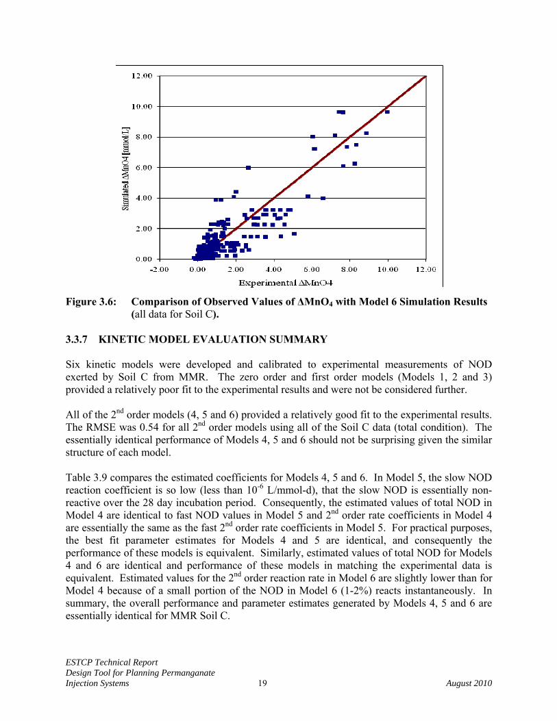
data for Soil C) Figure 3.6: Comparison of Observed Values of ΔMnO4 with Model 6 Simulation Results (all
data for Soil C) Figure 4.1: Location of MMR on Cape Cod, Massachusetts Figure 4.2: Plume Distribution of MMR (grey area represent MMR, red line represent plume
boundary, AFCEE 2007b) Figure 4.3: CS-10 Plume (grey area represent MMR, red line represent plume boundary,
AFCEE 2007b) Figure 4.4: Cross Section of Pilot Test Area (CH2M Hill 2007) Figure 4.5: Plan-View of MMR Pilot Test Simulation Grid Figure 4.6: Profile-View of MMR Pilot Test Simulation Grid Figure 4.7: Cross-Section View of Permeability Distribution Figure 4.8: Plan-View of 15th Layer of Model Showing and Injection and Monitoring Wells Figure 4.9: Front View of 50th Row of Model Showing Injection and Monitoring Wells Figure 4.10: Profile-View of Contaminant and Permanganate Distribution at 6, 18, 30 and 90
Days of Simulation with Scenario 4 (deep red indicate high concentration) Figure 5.1: Hypothetical Injection Grid Showing Model Domain Subarea Figure 5.2: Model Domain for Base Case Condition. Figure 5.3: Horizontal Hydraulic Conductivity, MnO4, NODI, NODS and Contaminant
Distributions in Top Layer of Aquifer at 120 days after Injection for Moderately Heterogeneous Aquifer when Wells 1-5 are Injected with SFV = SFM = 0.25
Figure 5.4: Horizontal Hydraulic Conductivity, MnO4, NODI, NODS and Contaminant Distributions in Last Row of Aquifer at 120 days after Injection for Moderately Heterogeneous Aquifer when Wells 1-5 are Injected with SFV = SFM = 0.25
Figure 5.5: Variation in Aquifer Volume Contact Efficiency and Contaminant Mass Treatment Efficiency (EM) with Time where Fluid Injection Volume is held Constant (SFV=0.25) and MnO4 Mass Varies (SFM varies from 0.1 to 1.0)
Figure 5.6: Variation in Aquifer Volume Contact Efficiency (EV) and Fraction Unreacted MnO4 (U) at 180 days after Injection with Mass and Volume Scaling Factors
Figure 5.7: Effect of Well Spacing on EV and U at 180 days for SFV = SFM in a Medium Heterogeneity Aquifer
Figure 5.8: Effect of Reinjection on EV and U at 180 days for SFV = SFM in a Medium Heterogeneity Aquifer. Well spacing = 3 m.
Figure 5.9: Effect of NOD Kinetic Parameters on EV and U at 180 days for SFV=SFM: (a) Slow NOD Reaction Rate (K2S); (b) Total NOD; and (c) Fraction NODI.
ix
Figure 5.10: Effect of Initial Contaminant Concentration (a) and Contaminant Retardation factor (b) on EV, EM and U at 180 days for SFV=SFM.
Figure 5.11: Effect of Low, Medium and High Aquifer Heterogeneity on EV, EM and U at 180 days (SFV = SFM)
Figure 6.1: Comparison of CDISCO, RT3D and 1D Analytical Solutions of Non-Reactive Solute Transport Away from a Single Injection Well at 1 day after Injection
Figure 6.2: Comparison of CDISCO and RT3D Simulations of MnO4, NODI, NODS and Contaminant Concentration at 10 days after Injection for αL =0.1 m.
Figure 6.3: Non-Reactive Solute Concentrations versus Radial Distance from Injection Well Generated in 3D Heterogeneous RT3D Simulation.
Figure 6.4: Comparison of CDISCO Simulation (αL = 1.5 m) and Spatially Averaged Concentrations from 3D RT3D Simulation
Figure 6.5: Comparison of Model Results at 10 days after Injection for 1-D Homogeneous CDISCO Simulation and 3-D spatially Heterogeneous RT3D Simulation for: (a) MnO4; (b) NODI; (c) NODS and Contaminant
Figure 6.6: Typical Output from Permanganate Transport Model Figure 6.7: Typical Output from Injection Scenario Cost Comparison Figure 6.8: Effect of Overlap Factor (OF) on Aquifer Volume Contact Efficiency (EV) and
Contaminant Mass Treatment Efficiency (EM).
ESTCP Technical Report Design Tool for Planning Permanganate Injection Systems 1 August 2010
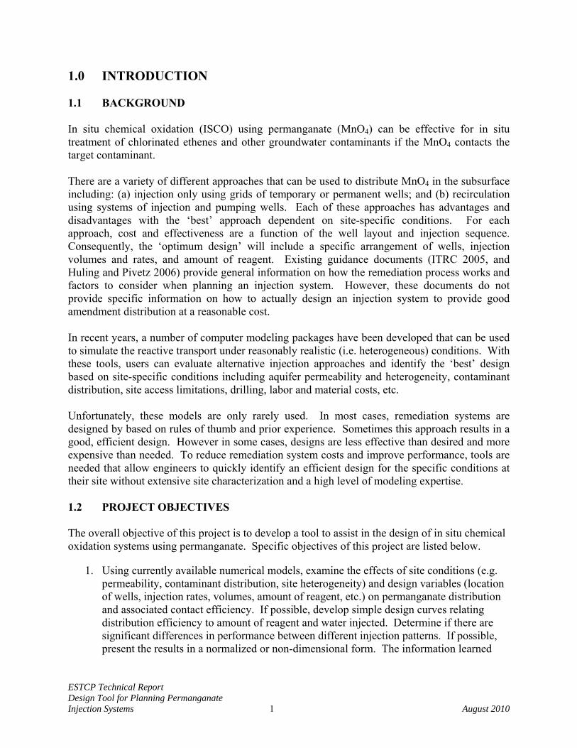
1.0 INTRODUCTION 1.1 BACKGROUND In situ chemical oxidation (ISCO) using permanganate (MnO4) can be effective for in situ treatment of chlorinated ethenes and other groundwater contaminants if the MnO4 contacts the target contaminant. There are a variety of different approaches that can be used to distribute MnO4 in the subsurface including: (a) injection only using grids of temporary or permanent wells; and (b) recirculation using systems of injection and pumping wells. Each of these approaches has advantages and disadvantages with the ‘best’ approach dependent on site-specific conditions. For each approach, cost and effectiveness are a function of the well layout and injection sequence. Consequently, the ‘optimum design’ will include a specific arrangement of wells, injection volumes and rates, and amount of reagent. Existing guidance documents (ITRC 2005, and Huling and Pivetz 2006) provide general information on how the remediation process works and factors to consider when planning an injection system. However, these documents do not provide specific information on how to actually design an injection system to provide good amendment distribution at a reasonable cost. In recent years, a number of computer modeling packages have been developed that can be used to simulate the reactive transport under reasonably realistic (i.e. heterogeneous) conditions. With these tools, users can evaluate alternative injection approaches and identify the ‘best’ design based on site-specific conditions including aquifer permeability and heterogeneity, contaminant distribution, site access limitations, drilling, labor and material costs, etc. Unfortunately, these models are only rarely used. In most cases, remediation systems are designed by based on rules of thumb and prior experience. Sometimes this approach results in a good, efficient design. However in some cases, designs are less effective than desired and more expensive than needed. To reduce remediation system costs and improve performance, tools are needed that allow engineers to quickly identify an efficient design for the specific conditions at their site without extensive site characterization and a high level of modeling expertise. 1.2 PROJECT OBJECTIVES The overall objective of this project is to develop a tool to assist in the design of in situ chemical oxidation systems using permanganate. Specific objectives of this project are listed below.
1. Using currently available numerical models, examine the effects of site conditions (e.g. permeability, contaminant distribution, site heterogeneity) and design variables (location of wells, injection rates, volumes, amount of reagent, etc.) on permanganate distribution and associated contact efficiency. If possible, develop simple design curves relating distribution efficiency to amount of reagent and water injected. Determine if there are significant differences in performance between different injection patterns. If possible, present the results in a normalized or non-dimensional form. The information learned

ESTCP Technical Report Design Tool for Planning Permanganate Injection Systems 2 August 2010
from the modeling will provide guidance to design tool users in selection of important design parameters (e.g., pore volumes of injection fluid, amount of reagent, etc.).
2. Develop a simple, spreadsheet-based tool to assist in the design of MnO4 injection systems. This design tool will allow designers to evaluate the effect of different variables (well spacing, amount of reagent and water, injection rate, etc.) on remediation system cost and expected performance. Experienced users who have already compiled the input data for their site (e.g. permeability, NOD, contaminant concentrations) should be able to quickly develop and evaluate several alternative designs.
1.3 STAKEHOLDER / END-USER ISSUES The primary objective of this project was to develop a design tool that is easy to learn, simple to use, and widely applied. The design tool is structured to allow new users to download the required materials, and complete a preliminary injection system design in a few hours without extensive groundwater modeling experience. However, users are expected to be familiar with basic fundamentals of groundwater flow, solute transport, and ISCO using MnO4. The design tool and guidance document are available for download from one or more websites.
ESTCP Technical Report Design Tool for Planning Permanganate Injection Systems 3 August 2010
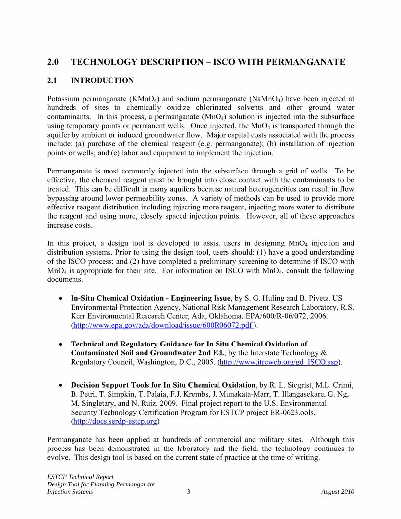
2.0 TECHNOLOGY DESCRIPTION – ISCO WITH PERMANGANATE 2.1 INTRODUCTION Potassium permanganate (KMnO4) and sodium permanganate (NaMnO4) have been injected at hundreds of sites to chemically oxidize chlorinated solvents and other ground water contaminants. In this process, a permanganate (MnO4) solution is injected into the subsurface using temporary points or permanent wells. Once injected, the MnO4 is transported through the aquifer by ambient or induced groundwater flow. Major capital costs associated with the process include: (a) purchase of the chemical reagent (e.g. permanganate); (b) installation of injection points or wells; and (c) labor and equipment to implement the injection. Permanganate is most commonly injected into the subsurface through a grid of wells. To be effective, the chemical reagent must be brought into close contact with the contaminants to be treated. This can be difficult in many aquifers because natural heterogeneities can result in flow bypassing around lower permeability zones. A variety of methods can be used to provide more effective reagent distribution including injecting more reagent, injecting more water to distribute the reagent and using more, closely spaced injection points. However, all of these approaches increase costs. In this project, a design tool is developed to assist users in designing MnO4 injection and distribution systems. Prior to using the design tool, users should: (1) have a good understanding of the ISCO process; and (2) have completed a preliminary screening to determine if ISCO with MnO4 is appropriate for their site. For information on ISCO with MnO4, consult the following documents.
• In-Situ Chemical Oxidation - Engineering Issue, by S. G. Huling and B. Pivetz. US Environmental Protection Agency, National Risk Management Research Laboratory, R.S. Kerr Environmental Research Center, Ada, Oklahoma. EPA/600/R-06/072, 2006. (http://www.epa.gov/ada/download/issue/600R06072.pdf ).
• Technical and Regulatory Guidance for In Situ Chemical Oxidation of
Contaminated Soil and Groundwater 2nd Ed., by the Interstate Technology & Regulatory Council, Washington, D.C., 2005. (http://www.itrcweb.org/gd_ISCO.asp).
• Decision Support Tools for In Situ Chemical Oxidation, by R. L. Siegrist, M.L. Crimi, B. Petri, T. Simpkin, T. Palaia, F.J. Krembs, J. Munakata-Marr, T. Illangasekare, G. Ng, M. Singletary, and N. Ruiz. 2009. Final project report to the U.S. Environmental Security Technology Certification Program for ESTCP project ER-0623.ools. (http://docs.serdp-estcp.org)
Permanganate has been applied at hundreds of commercial and military sites. Although this process has been demonstrated in the laboratory and the field, the technology continues to evolve. This design tool is based on the current state of practice at the time of writing.

ESTCP Technical Report Design Tool for Planning Permanganate Injection Systems 4 August 2010
2.2 PROCEDURES FOR INJECTING PERMANGANATE ISCO projects using permanganate typically, but not always, involve the following steps: (1) installation of injection wells and associated equipment; (2) preparation of a dilute reagent solution from solid KMnO4 or a concentrated NaMnO4 solution; and (3) injection of the reagent solution. The reagent can be injected through the end of a direct push rod, through temporary 1-inch direct-push wells, or through permanent 2-inch or 4-inch conventionally-drilled wells. The selection of the most appropriate method for installing injection points depends on site-specific conditions including drilling costs, flow rate per well, and volume of fluid that must be injected. Permanganate can be distributed 5, 10, or 25 ft away from the injection point. However, achieving effective distribution often requires injecting large volumes of water. Depending on the injection well layout and formation permeability, water injection can require an hour to several days per well. As a consequence, several wells may be injected at one time using a simple injection system manifold. The primary design variables that must be considered when planning a MnO4 injection project are:
(1) spatial arrangement of the injection points; (2) type and physical construction of the injection points or wells; (3) amount of MnO4 and water to inject; (4) reinjection frequency; and (5) additional labor and equipment required for mixing and injection.
Each of these variables has an important influence on both the cost and effectiveness of the injection project. 2.2.1 ARRANGEMENT OF INJECTION POINTS There are two general approaches used to distribute chemical reagents through the subsurface: (a) recirculation systems; and (b) injection only systems. Recirculation systems can be effective in distributing reagents significant distances through the subsurface in certain situations, allowing the use of fewer injection points. These systems are particularly useful where drilling costs are high or site access limitations restrict injection point installation. Recirculation systems can also be designed to minimize the physical displacement of contaminants by injection water. However, capital and operating costs of recirculation systems are often higher due to the more complex equipment and piping requirements and higher operation and maintenance (O&M) costs. In many cases, the design of recirculation systems is more complicated and may require the use of a site specific groundwater model. Injection only systems are most useful when drilling and site access conditions allow installation of rows or grids of injection points. Under these conditions, capital and O&M costs are often lower for injection only systems. The design of injection only systems can also be simplified by generating a ‘standard’ design for a small group of injection points which is then replicated throughout the site. The design tool described in this document has been developed to assist

ESTCP Technical Report Design Tool for Planning Permanganate Injection Systems 5 August 2010
users in the design of injection only systems for distributing chemical reagents using grids of injection points or wells. Once the target treatment zone has been defined, the user must then select an injection point spacing. Selecting the best well spacing can be complicated. Increasing the separation between injection wells reduces the number of wells, reducing drilling costs. However, a larger well spacing can also increase the time required for injection, increasing labor costs. It may also be more difficult to uniformly distribute the reagent throughout the treatment zone using fewer, widely spaced injection points. In many cases, an intermediate well spacing results in the lowest total cost with reasonably good reagent distribution throughout the target treatment zone. The design tool provides output illustrating the effect of well spacing on distribution efficiency and comparative costs allowing the designer to select a well spacing that best meets project objectives. 2.2.2 INJECTION POINT CONSTRUCTION MnO4 solutions can be injected through the end of a direct push rod, through temporary 1-inch direct-push wells, or through permanent 2-inch or 4-inch conventionally-drilled wells. The selection of the most appropriate method for installing injection points depends on site-specific conditions including drilling costs, flow rate per well, and volume of fluid that must be injected. When the contamination extends over a significant vertical extent, it may be desirable to install several shorter screened wells to target specific intervals. This allows a known quantity of reagent to be injected in each interval. However, this also increases injection system cost and complexity. 2.2.3 AMOUNT OF WATER AND CHEMICAL REAGENT TO INJECT MnO4 is transported in the subsurface by flowing groundwater. Consequently, sufficient water must be injected to transport the MnO4 throughout the target treatment zone. The amount of MnO4 required is determined by the target treatment volume and the oxidant demand of the aquifer material. MnO4 distribution in the aquifer can be enhanced by injecting more chemical reagent and/or more water. However, injecting additional reagent increases material costs and the potential for off-site migration of unreacted MnO4. Injecting additional water increases labor costs. The CDISCO design tool presented in Section 6 can be used to estimate the amount of reagent and water to inject. 2.2.4 REINJECTION FREQUENCY Following injection, MnO4 is consumed through reactions with the contaminant and Natural Oxidant Demand (NOD) associated with the aquifer material. To improve performance, additional MnO4 may be injected. Section 5.4 presents information on the relative benefits of multiple injections on contaminant treatment.

ESTCP Technical Report Design Tool for Planning Permanganate Injection Systems 6 August 2010
2.2.5 ADDITIONAL LABOR AND EQUIPMENT REQUIRED The major capital costs for MnO4 injection are associated with injection point installation, reagent purchase and labor during the injection. However, there are a number of other factors that can influence the final project cost including mobilization, setup of injection equipment (e.g. pumps, meters, etc.), injection water supply, and site cleanup. These costs are not closely related to the specific injection design. However, they can have a significant impact on the final project cost. In the design tool, costs for engineering and permitting, mobilization, equipment setup, water supply and cleanup/demobilization are entered as fixed costs.
ESTCP Technical Report Design Tool for Planning Permanganate Injection Systems 7 August 2010
3.0 PERMANGANATE CONSUMPTION BY AQUIFER MATERIAL 3.1 INTRODUCTION When MnO4 is injected into the subsurface, a portion of the material reacts with the target contaminant and a portion reacts with the aquifer material. The amount of permanganate that reacts with non-target chemicals is often referred to as the natural oxidant demand (NOD). When estimating the required amount of reagent to inject, designers must account for both permanganate consumed by the target chemicals and the NOD. If the NOD is not considered, the permanganate will be depleted more rapidly than expected and treatment efficiency may be less than desired. 3.2 FATE AND TRANSPORT OF PERMANGANATE IN THE SUBSURFACE Permanganate has been used for wastewater and drinking water treatment for many years (Steel and McGhee 1979; Eilbeck and Mattock 1987). In contrast, permanganate has been used for groundwater remediation for less than 20 years. However, recent work has shown permanganate to be an effective oxidant for treatment of chlorinated solvents (perchloroethene [PCE] and trichloroethene [TCE]) and aromatic hydrocarbons (naphthalene, phenanthrene, pyrene and phenols) (Vella et al. 1990; Leung et al. 1992; Vella and Veronda 1992; Gates et al. 1995, 2001; Yan and Schwartz 1996; 1999; Schnarr et al. 1998; West et al. 1998; Siegrist et al. 1998a, b, 2000, 2001; Lowe et al. 1999). Representative reactions illustrating the oxidation of PCE (C2Cl4) and TCE (C2HCl3) by permanganate are shown below. C2Cl4 + 11/3 MnO4
- 11/3 MnO2(s) + 2CO2 + 22/3 H+ + 4Cl- (PCE) C2HCl3 + 2MnO4
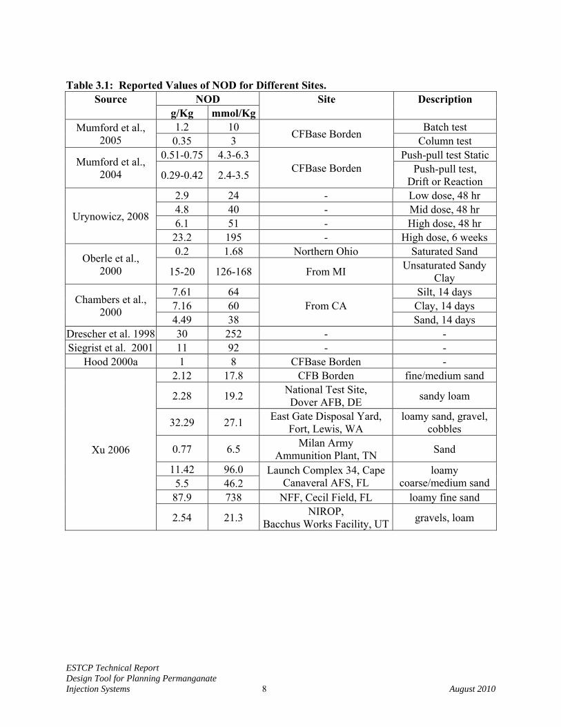
- 2MnO2(s) + 2CO2 + H+ + 3Cl- (TCE) Based on this stochiometry, 1.81 g of permanganate is needed to degrade 1 g of TCE, releasing 1.32 g of manganese dioxide, 0.67 g of carbon dioxide and 0.81 g of Cl- (Siegrist et al. 2001). 3.2.1 NATURAL OXIDANT DEMAND (NOD) In many cases, the NOD controls the amount of reagent which must be injected for effective treatment (Marvin et al. 2002). NOD is exerted when permanganate reacts with a variety of naturally occurring materials including ferrous iron, sulfides and natural organic carbon. NOD is commonly measured by reacting aquifer material with a permanganate solution and measuring change in permanganate concentration over time. NOD is typically reported as mass of permanganate consumed per unit mass of aquifer solids (Siegrist et al. 2000; Marvin et al. 2002). Efforts are underway to standardize the NOD test procedure (ASTM 2007). However, this standard protocol has only been used by a few investigators and published values of NOD have been measured under a range of experimental conditions. Table 3.1 shows the measured values of NOD value for several different sites and experimental conditions. Reported NOD values range from 0.3 to 88 g MnO4 / Kg indicating NOD can vary dramatically between sites.
ESTCP Technical Report Design Tool for Planning Permanganate Injection Systems 8 August 2010
Table 3.1: Reported Values of NOD for Different Sites.
Source NOD Site Description g/Kg mmol/Kg
Mumford et al., 2005
1.2 10 CFBase Borden Batch test 0.35 3 Column test
Mumford et al., 2004
0.51-0.75 4.3-6.3 CFBase Borden
Push-pull test Static
0.29-0.42 2.4-3.5 Push-pull test, Drift or Reaction
Urynowicz, 2008
2.9 24 - Low dose, 48 hr 4.8 40 - Mid dose, 48 hr 6.1 51 - High dose, 48 hr 23.2 195 - High dose, 6 weeks
Oberle et al., 2000
0.2 1.68 Northern Ohio Saturated Sand
15-20 126-168 From MI Unsaturated Sandy Clay
Chambers et al., 2000
7.61 64 From CA
Silt, 14 days 7.16 60 Clay, 14 days 4.49 38 Sand, 14 days
Drescher et al. 1998 30 252 - - Siegrist et al. 2001 11 92 - -
Hood 2000a 1 8 CFBase Borden -
Xu 2006
2.12 17.8 CFB Borden fine/medium sand
2.28 19.2 National Test Site, Dover AFB, DE sandy loam
32.29 27.1 East Gate Disposal Yard, Fort, Lewis, WA
loamy sand, gravel, cobbles
0.77 6.5 Milan Army Ammunition Plant, TN Sand
11.42 96.0 Launch Complex 34, Cape Canaveral AFS, FL
loamy coarse/medium sand 5.5 46.2
87.9 738 NFF, Cecil Field, FL loamy fine sand
2.54 21.3 NIROP, Bacchus Works Facility, UT gravels, loam
ESTCP Technical Report Design Tool for Planning Permanganate Injection Systems 9 August 2010
3.2.2 MODELING APPROACHES A number of different modeling approaches have been applied to describe the kinetics of MnO4 consumption by NOD (Hood and Thomson, 2000; Reitsma and Dai, 2001; Mumford, 2002; Xu, 2006; Jones, 2007; Hønning et al., 2007; Urynowicz et al., 2008). Potentially the simplest approach would be to assume that the reaction is instantaneous and NOD must be completely consumed before the MnO4 can be transported away from the injection point. However, this approach would likely over-estimate MnO4 consumption since a portion of the NOD may react slowly. The most common modeling approach has been to simulate the reaction between M and NOD (N) as a 2nd order reaction (Zhang and Schwartz 2000, Xu 2006),
dM/dt = - kN M N where kN is the 2nd order rate of reaction between MnO4 and NOD. Zhang and Schwartz 2000 used a kN value of 450 M-1 s-1 which is much faster than the rate of contaminant oxidation and results in essentially complete depletion of the NOD before MnO4 will migrate through the aquifer. However in batch experiments conducted by Hønning et al. (2007), the long-term consumption of MnO4 by NOD could not be described by a single 1st order decay rate. During the first few hours of the reaction, MnO4 decreased at rates of 0.05 – 0.5 h-1 and then declined more slowly. Recent work has shown that NOD is composed of several components or fractions with varying reactivity (Mumford et al., 2005; Xu, 2006; Urynowicz et al., 2008). Ideally, NOD would be represented with a continuum of reaction rates where the less reactive fraction becomes progressively more important as the more reactive NOD fraction is depleted. However, modeling studies by Xu (2006) and Urynowicz et al. (2008) suggest that MnO4 consumption by NOD can be reasonably well described assuming the NOD is composed of one fast and one slow fraction. In batch experiments conducted by Xu (2006), a fraction of the NOD was depleted in a few hours followed by much slower degradation, where the slow NOD reaction rate varied from 0.014 to 0.72 L/mmol-day with a median value of 0.077 L/mmol-day. In batch experiments conducted by Urynowicz et al. (2008), the fast NOD appeared to be consumed with about 48 hours, followed by slower depletion of MnO4 at rates of 0.024 to 0.13 d-1, depending MnO4 dose. 3.3 KINETIC MODEL EVALUATION At present, there is no general consensus on the best approach for simulating MnO4 consumption by NOD. However, there does seem to be some agreement that: (1) NOD is often composed of different components or fractions; (2) some components react fairly quickly (minutes to hours); (3) some components react more slowly (days to months); and (4) the effective NOD is a function of permanganate concentration with higher concentrations resulting in higher effective NOD. In this project, groundwater flow, transport and reaction models (MODFLOW and RT3D) are used to evaluate the effect of injection conditions on treatment efficiency in a three dimensional (3D) heterogeneous aquifer. The models must adequately represent the kinetics of MnO4 consumption by NOD, but must be relatively simple to implement and not result in an excessive
ESTCP Technical Report Design Tool for Planning Permanganate Injection Systems 10 August 2010
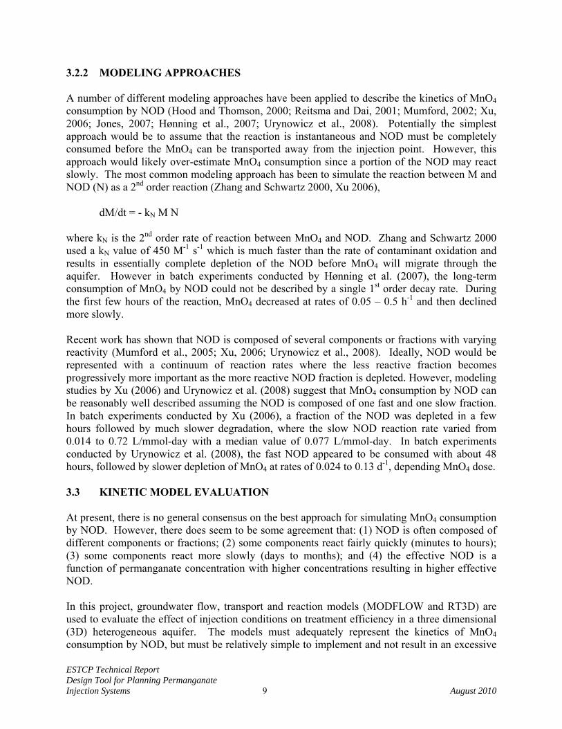
computational burden. Given that there is no one modeling approach that is generally accepted, six different approaches were evaluated for describing NOD kinetics. Each of the modeling approaches was calibrated to match the results of all batch NOD incubations with a sample of aquifer material (Soil C) from the Massachusetts Military Reservation (MMR). Experimental data was provided by Dr. Michelle Crimi of Clarkson University. The model performance was then evaluated based on a visual comparison of measured and simulated NOD, and statistical measures describing the goodness of fit. The batch incubations were conducted in glass jars with varying amounts of aquifer material and KMnO4 (500, 1000 and 5000 mg/L), aquifer material (16, 32 and 48 g) and water (10, 20 and 30 g) (see Table 3.2 for the different treatments). In addition, three different mixing conditions were evaluated: (1) complete mixing; (2) mixing once per day; and (3) static (mix only before sample collection). MnO4 concentration was typically measured approximately 16 times over the 28 day incubation period resulting in a total of 834 MnO4 measurements. Table 3.2: Batch Experimental Conditions of Each Treatment.
Treatment Initial KMnO4 Conc. (mg/L) Mass Solids (g) Mass Water (g)
1 5000 16 30 2 1000 16 30 3 500 16 30 4 5000 32 20 5 1000 32 20 6 500 32 20 7 5000 48 10 8 1000 48 10 9 500 48 10
The kinetic models evaluated in this work are summarized below. Each model was coded into MS Excel as a Visual BASIC subroutine using a 4th order Runge-Kutta solution of the ordinary differential equations (ODE’s). An initial set of model coefficients was assumed, and used to predict the variation in MnO4 concentrations vs. time for all incubations of Soil C. The goodness of fit was then evaluated as the root mean square error (RMSE) between simulated and measured MnO4 concentration in all incubations of Soil C. Best fit parameter values were found using the Solver function in Excel to search for the parameter set that resulted in the smallest RMSE. Best fit parameter values were obtained for the three soils for each mixing condition (complete mix, mix once per day, and static) and a fourth condition where all the data for the soil was pooled together, ignoring mixing condition. For each of the models, the ME (Mean Error) and the RSME are presented as indicators of goodness of fit. The best model should have a value of ME and RMSE close to zero. Graphs are also presented showing the measured change in MnO4 concentration from the start of the incubation (ΔMnO4) vs. simulated ΔMnO4 with the pooled data for Soil C. Ideally, the experimental measurements should cluster around the 45º line indicating a 1:1 match between measured and simulated values. Clustering of data away from the 45º line indicates that there is some trend in the experimental results that is not captured by the kinetic model.
ESTCP Technical Report Design Tool for Planning Permanganate Injection Systems 11 August 2010
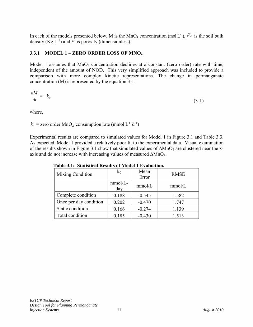
In each of the models presented below, M is the MnO4 concentration (mol L-1), Bρ is the soil bulk density (Kg L-1) and n is porosity (dimensionless). 3.3.1 MODEL 1 – ZERO ORDER LOSS OF MNO4 Model 1 assumes that MnO4 concentration declines at a constant (zero order) rate with time, independent of the amount of NOD. This very simplified approach was included to provide a comparison with more complex kinetic representations. The change in permanganate concentration (M) is represented by the equation 3-1.
0dM kdt
= − (3-1)
where,
-1 -14 = zero order MnO consumption rate (mmol L d )0k
Experimental results are compared to simulated values for Model 1 in Figure 3.1 and Table 3.3. As expected, Model 1 provided a relatively poor fit to the experimental data. Visual examination of the results shown in Figure 3.1 show that simulated values of ΔMnO4 are clustered near the x-axis and do not increase with increasing values of measured ΔMnO4. Table 3.1: Statistical Results of Model 1 Evaluation.
Mixing Condition k0 Mean Error RMSE
mmol/L-day mmol/L mmol/L
Complete condition 0.188 -0.545 1.582 Once per day condition 0.202 -0.470 1.747 Static condition 0.166 -0.274 1.139 Total condition 0.185 -0.430 1.513
ESTCP Technical Report Design Tool for Planning Permanganate Injection Systems 12 August 2010
Figure 3.1: Comparison of Observed Values of ΔMnO4 with Model 1 Simulation Results
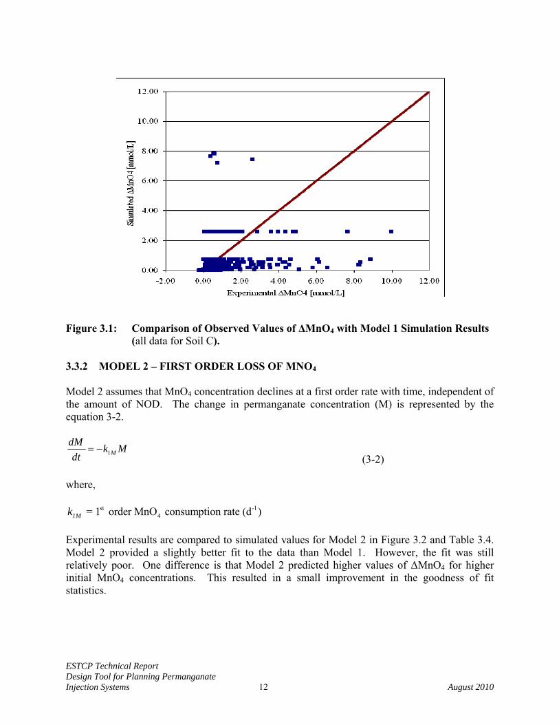
(all data for Soil C). 3.3.2 MODEL 2 – FIRST ORDER LOSS OF MNO4 Model 2 assumes that MnO4 concentration declines at a first order rate with time, independent of the amount of NOD. The change in permanganate concentration (M) is represented by the equation 3-2.
1MdM k Mdt
= − (3-2)
where,
st -14 = 1 order MnO consumption rate (d )1Mk
Experimental results are compared to simulated values for Model 2 in Figure 3.2 and Table 3.4. Model 2 provided a slightly better fit to the data than Model 1. However, the fit was still relatively poor. One difference is that Model 2 predicted higher values of ΔMnO4 for higher initial MnO4 concentrations. This resulted in a small improvement in the goodness of fit statistics.
ESTCP Technical Report Design Tool for Planning Permanganate Injection Systems 13 August 2010
Table 3.4: Statistical Results of Model 2 Evaluation.
Mixing Condition k1M Mean Error RMSE 1/day mmol/L mmol/L Complete condition 0.014 -0.587 1.472 Once per day condition 0.017 -0.458 1.530 Static condition 0.013 -0.291 0.955 Total condition 0.015 -0.446 1.349
Figure 3.2: Comparison of Observed Values of ΔMnO4 with Model 2 Simulation Results
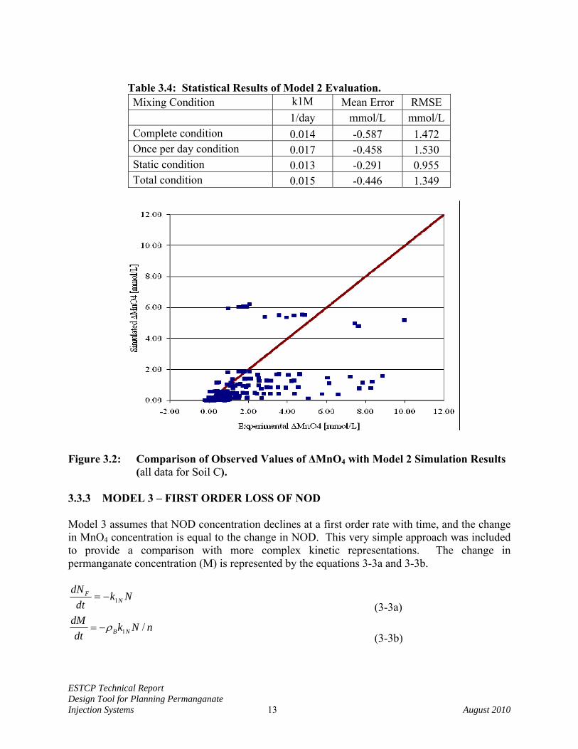
(all data for Soil C). 3.3.3 MODEL 3 – FIRST ORDER LOSS OF NOD Model 3 assumes that NOD concentration declines at a first order rate with time, and the change in MnO4 concentration is equal to the change in NOD. This very simple approach was included to provide a comparison with more complex kinetic representations. The change in permanganate concentration (M) is represented by the equations 3-3a and 3-3b.
1F
NdN k Ndt
= − (3-3a)
1 /B NdM k N ndt
ρ= − (3-3b)
ESTCP Technical Report Design Tool for Planning Permanganate Injection Systems 14 August 2010
where,
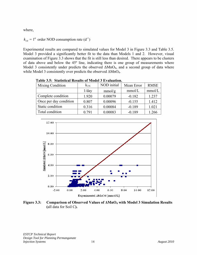
st -1= 1 order NOD consumption rate (d )1Nk Experimental results are compared to simulated values for Model 3 in Figure 3.3 and Table 3.5. Model 3 provided a significantly better fit to the data than Models 1 and 2. However, visual examination of Figure 3.3 shows that the fit is still less than desired. There appears to be clusters of data above and below the 45º line, indicating there is one group of measurements where Model 3 consistently under predicts the observed ΔMnO4, and a second group of data where while Model 3 consistently over predicts the observed ΔMnO4. Table 3.5: Statistical Results of Model 3 Evaluation.
Mixing Condition k1N NOD initial Mean Error RMSE 1/day mmol/g mmol/L mmol/LComplete condition 1.920 0.00079 -0.182 1.237 Once per day condition 0.807 0.00096 -0.155 1.412 Static condition 0.316 0.00084 -0.189 1.021 Total condition 0.791 0.00083 -0.189 1.266
Figure 3.3: Comparison of Observed Values of ΔMnO4 with Model 3 Simulation Results
(all data for Soil C).
ESTCP Technical Report Design Tool for Planning Permanganate Injection Systems 15 August 2010
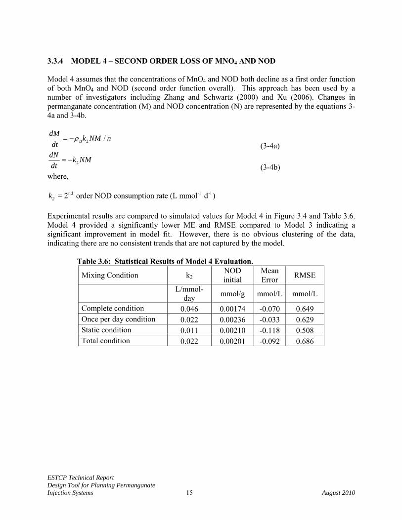
3.3.4 MODEL 4 – SECOND ORDER LOSS OF MNO4 AND NOD Model 4 assumes that the concentrations of MnO4 and NOD both decline as a first order function of both MnO4 and NOD (second order function overall). This approach has been used by a number of investigators including Zhang and Schwartz (2000) and Xu (2006). Changes in permanganate concentration (M) and NOD concentration (N) are represented by the equations 3-4a and 3-4b.
2 /BdM k NM ndt
ρ= − (3-4a)
2dN k NMdt
= − (3-4b)
where,
nd -1 -1 = 2 order NOD consumption rate (L mmol d )2k Experimental results are compared to simulated values for Model 4 in Figure 3.4 and Table 3.6. Model 4 provided a significantly lower ME and RMSE compared to Model 3 indicating a significant improvement in model fit. However, there is no obvious clustering of the data, indicating there are no consistent trends that are not captured by the model. Table 3.6: Statistical Results of Model 4 Evaluation.
Mixing Condition k2 NOD initial
Mean Error RMSE
L/mmol-day mmol/g mmol/L mmol/L
Complete condition 0.046 0.00174 -0.070 0.649 Once per day condition 0.022 0.00236 -0.033 0.629 Static condition 0.011 0.00210 -0.118 0.508 Total condition 0.022 0.00201 -0.092 0.686
ESTCP Technical Report Design Tool for Planning Permanganate Injection Systems 16 August 2010
Figure 3.4: Comparison of Observed Values of ΔMnO4 with Model 4 Simulation Results
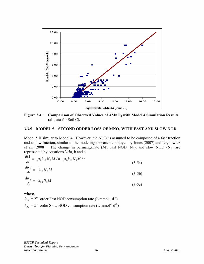
(all data for Soil C). 3.3.5 MODEL 5 – SECOND ORDER LOSS OF MNO4 WITH FAST AND SLOW NOD Model 5 is similar to Model 4. However, the NOD is assumed to be composed of a fast fraction and a slow fraction, similar to the modeling approach employed by Jones (2007) and Urynowicz et al. (2008). The change in permanganate (M), fast NOD (NF), and slow NOD (NS) are represented by equations 3-5a, b and c.
2 2/ /B F F B S SdM k N M n k N M ndt
ρ ρ= − − (3-5a)
2F
F FdN k N Mdt
= − (3-5b)
2S
S SdN k N Mdt
= − (3-5c)
where,
nd -1 -1
nd -1 -1
= 2 order Fast NOD consumption rate (L mmol d )
= 2 order Slow NOD consumption rate (L mmol d )2F
2S
k
k
ESTCP Technical Report Design Tool for Planning Permanganate Injection Systems 17 August 2010
Experimental results are compared to simulated values for Model 5 in Figure 3.5 and Table 3.7. RMSE values for Model 5 were very similar to Model 4 indicating that separation of the NOD into a fast and slow fraction did not significantly improve the model fit for the MMR soils. However, ME values were much lower. In addition, Model 5 run times were significantly longer than for Model 4. This was because the high reaction rates for fast NOD required a shorter computational time step. Table 3.7: Statistical Results of Model 5 Evaluation.
Mixing Condition k2F k2S Fraction Fast
NOD initial Mean Error RMSE
L/mmol-d L/mmol-d mmol/g mmol/L mmol/LComplete condition 0.0458 0.000001 0.15 0.0117 0.017 0.650 Once per day condition 0.0223 0.000001 0.14 0.0170 0.014 0.629 Static condition 0.0107 0.000005 0.16 0.0128 -0.015 0.508 Total condition 0.0220 0.000001 0.15 0.0132 -0.001 0.686
Figure 3.5: Comparison of Observed Values of ΔMnO4 with Model 5 Simulation Results
(all data for Soil C).
ESTCP Technical Report Design Tool for Planning Permanganate Injection Systems 18 August 2010
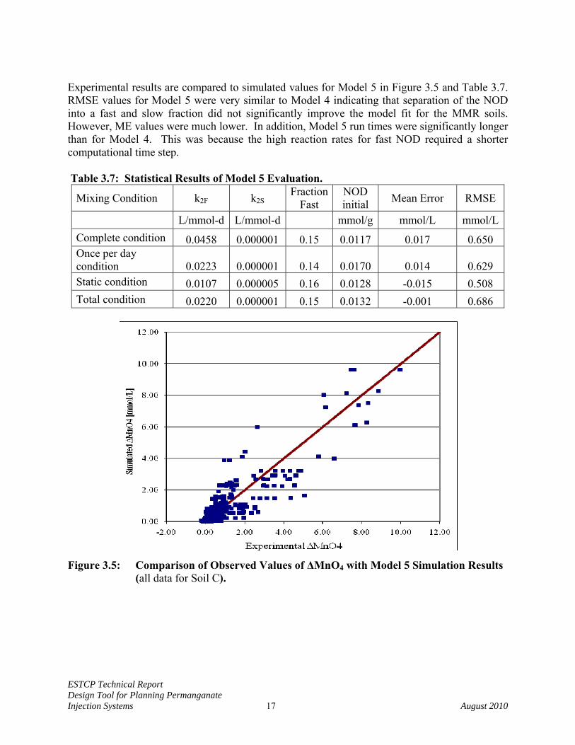
3.3.6 MODEL 6 – SECOND ORDER LOSS OF MNO4 WITH INSTANTANEOUS AND
SLOW NOD Model 6 is similar to Model 5. However, the reaction between MnO4 and fast NOD is assumed to occur so quickly, that it is essentially instantaneous. The instantaneous change in permanganate (M) and instantaneous NOD (NI) are calculated by an if then statement, When concentration of * /
* / 0 otherwise 0 * /I B
B I I I I B
M N nM M N n and N M and N N M n
ρρ ρ
>= − = = = −
Once the instantaneous reaction is complete, the change in permanganate (M) and slow NOD (NS) are calculated by solving equations 3-6a and 3-6b.
2 /B S SdM k N M ndt
ρ= − (3-6a)
2S
S SdN k N Mdt
= − (3-6b)
nd -1 -1 = 2 order Slow NOD consumption rate (L mmol d )2Sk Experimental results are compared to simulated values for Model 6 in Figure 3.6 and Table 3.8. Error statistics for Model 6 were very similar to Models 4 and 5 indicating that representing the reaction between ‘fast’ NOD and MnO4 as an instantaneous reaction did not significantly hurt model performance. However, Model 6 run times were significantly shorter than Model 5. This would be a major advantage when simulating complex 3D aquifers. Table 3.8: Statistical Results of Model 6 Evaluation
Mixing Condition k2S Fraction Instantaneous
NOD initial
Mean Error RMSE
L/mmol-day mmol/g mmol/L mmol/LComplete condition 0.0457 0.001 0.0017 -0.069 0.649 Once per day condition 0.0221 0.001 0.0024 -0.031 0.630 Static condition 0.0106 0.001 0.0021 -0.117 0.508 Total condition 0.0217 0.002 0.0020 -0.088 0.685
ESTCP Technical Report Design Tool for Planning Permanganate Injection Systems 19 August 2010
Figure 3.6: Comparison of Observed Values of ΔMnO4 with Model 6 Simulation Results
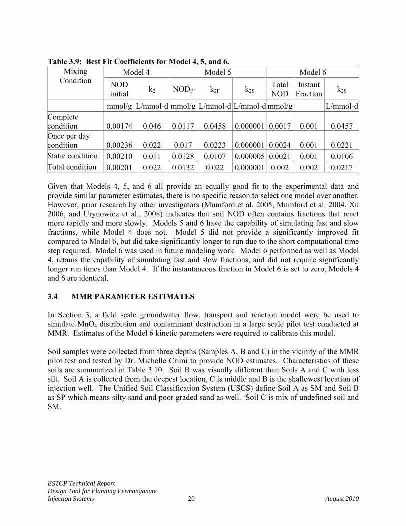
(all data for Soil C). 3.3.7 KINETIC MODEL EVALUATION SUMMARY Six kinetic models were developed and calibrated to experimental measurements of NOD exerted by Soil C from MMR. The zero order and first order models (Models 1, 2 and 3) provided a relatively poor fit to the experimental results and were not be considered further. All of the 2nd order models (4, 5 and 6) provided a relatively good fit to the experimental results. The RMSE was 0.54 for all 2nd order models using all of the Soil C data (total condition). The essentially identical performance of Models 4, 5 and 6 should not be surprising given the similar structure of each model. Table 3.9 compares the estimated coefficients for Models 4, 5 and 6. In Model 5, the slow NOD reaction coefficient is so low (less than 10-6 L/mmol-d), that the slow NOD is essentially non-reactive over the 28 day incubation period. Consequently, the estimated values of total NOD in Model 4 are identical to fast NOD values in Model 5 and 2nd order rate coefficients in Model 4 are essentially the same as the fast 2nd order rate coefficients in Model 5. For practical purposes, the best fit parameter estimates for Models 4 and 5 are identical, and consequently the performance of these models is equivalent. Similarly, estimated values of total NOD for Models 4 and 6 are identical and performance of these models in matching the experimental data is equivalent. Estimated values for the 2nd order reaction rate in Model 6 are slightly lower than for Model 4 because of a small portion of the NOD in Model 6 (1-2%) reacts instantaneously. In summary, the overall performance and parameter estimates generated by Models 4, 5 and 6 are essentially identical for MMR Soil C.
ESTCP Technical Report Design Tool for Planning Permanganate Injection Systems 20 August 2010
Table 3.9: Best Fit Coefficients for Model 4, 5, and 6.
Mixing Condition
Model 4 Model 5 Model 6 NOD initial k2 NODF k2F k2S Total
NOD Instant
Fraction k2S
mmol/g L/mmol-d mmol/g L/mmol-d L/mmol-d mmol/g L/mmol-dComplete condition 0.00174 0.046 0.0117 0.0458 0.000001 0.0017 0.001 0.0457 Once per day condition 0.00236 0.022 0.017 0.0223 0.000001 0.0024 0.001 0.0221 Static condition 0.00210 0.011 0.0128 0.0107 0.000005 0.0021 0.001 0.0106 Total condition 0.00201 0.022 0.0132 0.022 0.000001 0.002 0.002 0.0217 Given that Models 4, 5, and 6 all provide an equally good fit to the experimental data and provide similar parameter estimates, there is no specific reason to select one model over another. However, prior research by other investigators (Mumford et al. 2005, Mumford et al. 2004, Xu 2006, and Urynowicz et al., 2008) indicates that soil NOD often contains fractions that react more rapidly and more slowly. Models 5 and 6 have the capability of simulating fast and slow fractions, while Model 4 does not. Model 5 did not provide a significantly improved fit compared to Model 6, but did take significantly longer to run due to the short computational time step required. Model 6 was used in future modeling work. Model 6 performed as well as Model 4, retains the capability of simulating fast and slow fractions, and did not require significantly longer run times than Model 4. If the instantaneous fraction in Model 6 is set to zero, Models 4 and 6 are identical. 3.4 MMR PARAMETER ESTIMATES In Section 3, a field scale groundwater flow, transport and reaction model were be used to simulate MnO4 distribution and contaminant destruction in a large scale pilot test conducted at MMR. Estimates of the Model 6 kinetic parameters were required to calibrate this model. Soil samples were collected from three depths (Samples A, B and C) in the vicinity of the MMR pilot test and tested by Dr. Michelle Crimi to provide NOD estimates. Characteristics of these soils are summarized in Table 3.10. Soil B was visually different than Soils A and C with less silt. Soil A is collected from the deepest location, C is middle and B is the shallowest location of injection well. The Unified Soil Classification System (USCS) define Soil A as SM and Soil B as SP which means silty sand and poor graded sand as well. Soil C is mix of undefined soil and SM.
ESTCP Technical Report Design Tool for Planning Permanganate Injection Systems 21 August 2010
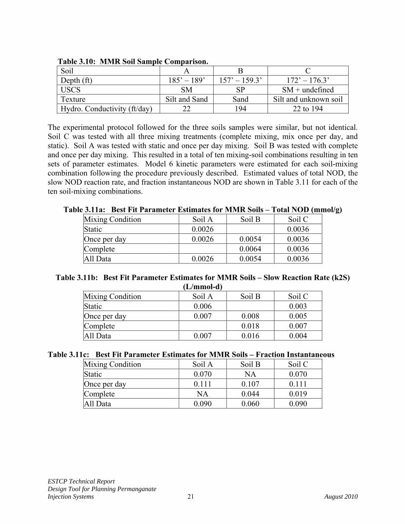
Table 3.10: MMR Soil Sample Comparison.
Soil A B C Depth (ft) 185’ – 189’ 157’ – 159.3’ 172’ – 176.3’ USCS SM SP SM + undefined Texture Silt and Sand Sand Silt and unknown soil Hydro. Conductivity (ft/day) 22 194 22 to 194
The experimental protocol followed for the three soils samples were similar, but not identical. Soil C was tested with all three mixing treatments (complete mixing, mix once per day, and static). Soil A was tested with static and once per day mixing. Soil B was tested with complete and once per day mixing. This resulted in a total of ten mixing-soil combinations resulting in ten sets of parameter estimates. Model 6 kinetic parameters were estimated for each soil-mixing combination following the procedure previously described. Estimated values of total NOD, the slow NOD reaction rate, and fraction instantaneous NOD are shown in Table 3.11 for each of the ten soil-mixing combinations.
Table 3.11a: Best Fit Parameter Estimates for MMR Soils – Total NOD (mmol/g) Mixing Condition Soil A Soil B Soil C Static 0.0026 0.0036 Once per day 0.0026 0.0054 0.0036 Complete 0.0064 0.0036 All Data 0.0026 0.0054 0.0036
Table 3.11b: Best Fit Parameter Estimates for MMR Soils – Slow Reaction Rate (k2S)
(L/mmol-d) Mixing Condition Soil A Soil B Soil C Static 0.006 0.003 Once per day 0.007 0.008 0.005 Complete 0.018 0.007 All Data 0.007 0.016 0.004
Table 3.11c: Best Fit Parameter Estimates for MMR Soils – Fraction Instantaneous
Mixing Condition Soil A Soil B Soil C Static 0.070 NA 0.070 Once per day 0.111 0.107 0.111 Complete NA 0.044 0.019 All Data 0.090 0.060 0.090
ESTCP Technical Report Design Tool for Planning Permanganate Injection Systems 22 August 2010
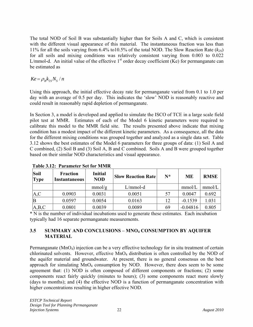
The total NOD of Soil B was substantially higher than for Soils A and C, which is consistent with the different visual appearance of this material. The instantaneous fraction was less than 11% for all the soils varying from 6.4% to10.5% of the total NOD. The Slow Reaction Rate (k2S) for all soils and mixing conditions was relatively consistent varying from 0.003 to 0.022 L/mmol-d. An initial value of the effective 1st order decay coefficient (Ke) for permanganate can be estimated as
2 /B S SKe k N nρ= Using this approach, the initial effective decay rate for permanganate varied from 0.1 to 1.0 per day with an average of 0.5 per day. This indicates the ‘slow’ NOD is reasonably reactive and could result in reasonably rapid depletion of permanganate. In Section 3, a model is developed and applied to simulate the ISCO of TCE in a large scale field pilot test at MMR. Estimates of each of the Model 6 kinetic parameters were required to calibrate this model to the MMR field site. The results presented above indicate that mixing condition has a modest impact of the different kinetic parameters. As a consequence, all the data for the different mixing conditions was grouped together and analyzed as a single data set. Table 3.12 shows the best estimates of the Model 6 parameters for three groups of data: (1) Soil A and C combined, (2) Soil B and (3) Soil A, B and C combined. Soils A and B were grouped together based on their similar NOD characteristics and visual appearance. Table 3.12: Parameter Set for MMR
Soil Type
Fraction Instantaneous
Initial NOD Slow Reaction Rate N* ME RMSE
mmol/g L/mmol-d mmol/L mmol/LA,C 0.0903 0.0031 0.0051 57 0.0047 0.692 B 0.0597 0.0054 0.0163 12 -0.1539 1.031 A,B,C 0.0801 0.0039 0.0089 69 -0.04816 0.805
* N is the number of individual incubations used to generate these estimates. Each incubation typically had 16 separate permanganate measurements. 3.5 SUMMARY AND CONCLUSIONS – MNO4 CONSUMPTION BY AQUIFER
MATERIAL Permanganate (MnO4) injection can be a very effective technology for in situ treatment of certain chlorinated solvents. However, effective MnO4 distribution is often controlled by the NOD of the aquifer material and groundwater. At present, there is no general consensus on the best approach for simulating MnO4 consumption by NOD. However, there does seem to be some agreement that: (1) NOD is often composed of different components or fractions; (2) some components react fairly quickly (minutes to hours); (3) some components react more slowly (days to months); and (4) the effective NOD is a function of permanganate concentration with higher concentrations resulting in higher effective NOD.

ESTCP Technical Report Design Tool for Planning Permanganate Injection Systems 23 August 2010
Six different kinetic relationships were examined to identify the relationship that best fits the loss of permanganate in experimental incubations using soil C from MMR. The three models that included a second order relationship between permanganate concentration (M) and NOD concentration all provided an equally good fit to the experimental data. Model 6 was selected for future use based on its’ ability to fit the experimental data, ease of numerical solution, and flexibility in simulating NOD composed of rapidly and slowly reactive materials. Model 6 includes a fraction of NOD which instantaneously reacts with MnO4 and a slow NOD component which reacts with MnO4 by a second order relationship.
ESTCP Technical Report Design Tool for Planning Permanganate Injection Systems 24 August 2010
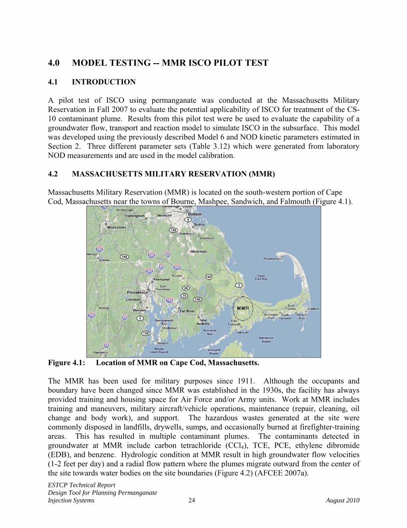
4.0 MODEL TESTING -- MMR ISCO PILOT TEST 4.1 INTRODUCTION A pilot test of ISCO using permanganate was conducted at the Massachusetts Military Reservation in Fall 2007 to evaluate the potential applicability of ISCO for treatment of the CS-10 contaminant plume. Results from this pilot test were be used to evaluate the capability of a groundwater flow, transport and reaction model to simulate ISCO in the subsurface. This model was developed using the previously described Model 6 and NOD kinetic parameters estimated in Section 2. Three different parameter sets (Table 3.12) which were generated from laboratory NOD measurements and are used in the model calibration. 4.2 MASSACHUSETTS MILITARY RESERVATION (MMR) Massachusetts Military Reservation (MMR) is located on the south-western portion of Cape Cod, Massachusetts near the towns of Bourne, Mashpee, Sandwich, and Falmouth (Figure 4.1).
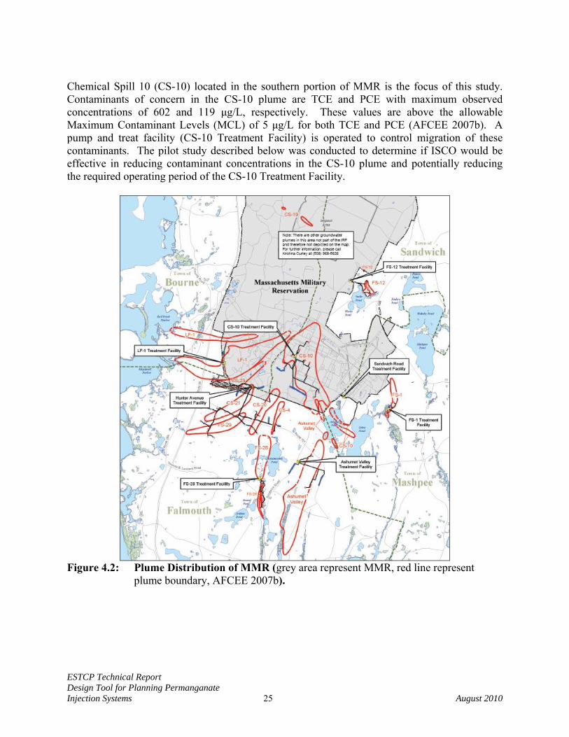
Figure 4.1: Location of MMR on Cape Cod, Massachusetts. The MMR has been used for military purposes since 1911. Although the occupants and boundary have been changed since MMR was established in the 1930s, the facility has always provided training and housing space for Air Force and/or Army units. Work at MMR includes training and maneuvers, military aircraft/vehicle operations, maintenance (repair, cleaning, oil change and body work), and support. The hazardous wastes generated at the site were commonly disposed in landfills, drywells, sumps, and occasionally burned at firefighter-training areas. This has resulted in multiple contaminant plumes. The contaminants detected in groundwater at MMR include carbon tetrachloride (CCl4), TCE, PCE, ethylene dibromide (EDB), and benzene. Hydrologic condition at MMR result in high groundwater flow velocities (1-2 feet per day) and a radial flow pattern where the plumes migrate outward from the center of the site towards water bodies on the site boundaries (Figure 4.2) (AFCEE 2007a).
ESTCP Technical Report Design Tool for Planning Permanganate Injection Systems 25 August 2010
Chemical Spill 10 (CS-10) located in the southern portion of MMR is the focus of this study. Contaminants of concern in the CS-10 plume are TCE and PCE with maximum observed concentrations of 602 and 119 μg/L, respectively. These values are above the allowable Maximum Contaminant Levels (MCL) of 5 μg/L for both TCE and PCE (AFCEE 2007b). A pump and treat facility (CS-10 Treatment Facility) is operated to control migration of these contaminants. The pilot study described below was conducted to determine if ISCO would be effective in reducing contaminant concentrations in the CS-10 plume and potentially reducing the required operating period of the CS-10 Treatment Facility.
Figure 4.2: Plume Distribution of MMR (grey area represent MMR, red line represent
plume boundary, AFCEE 2007b).

ESTCP Technical Report Design Tool for Planning Permanganate Injection Systems 26 August 2010
4.3 PILOT TEST The ISCO pilot test was conducted near monitor well 03MW1024 because of the relatively high TCE concentrations in this area and the opportunity to reduce future remediation costs. The geology of this site is similar to other portions of the CS-10 plume and other areas at MMR, potentially allowing results from this site to be extrapolated to other locations. The test area is also easily accessible for power supplies, equipment, personnel and is a secure location (CH2M Hill 2007).
Figure 4.3: CS-10 Plume (grey area represents MMR, red line represent plume boundary,
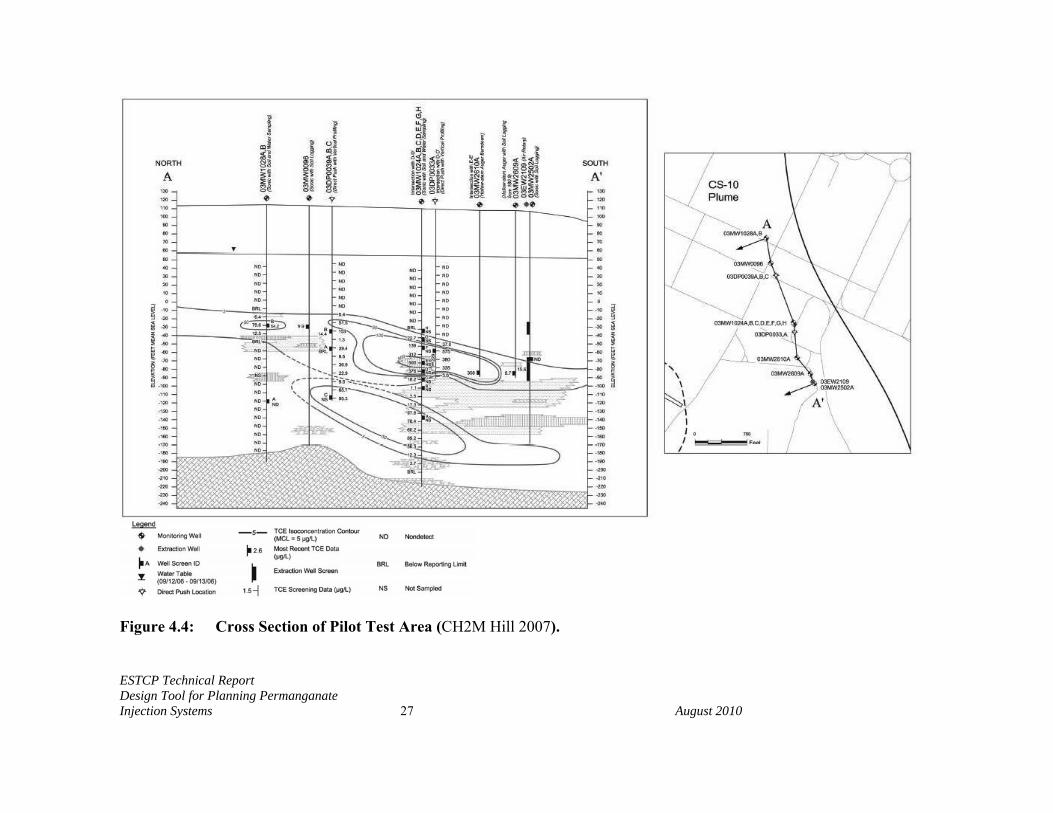
AFCEE 2007b). TCE contamination at the pilot test site is distributed in two major zones (Figure 4.4), a shallow zone extending from 150 to 205 feet below ground surface (ft bgs) with concentration ranging from TCE varying from 18 to 590 μg/L, and a deep zone extending from 230 to 295 ft bgs with TCE varying from 12 to 98 μg/L. Most of the aquifer material in pilot test area is sand. However, a fine sand /silty sand unit is located between 175 and 201 ft bgs, at approximately the same depth as the zone of maximum contaminant concentration (CH2M Hill 2007).
ESTCP Technical Report Design Tool for Planning Permanganate Injection Systems 27 August 2010
Figure 4.4: Cross Section of Pilot Test Area (CH2M Hill 2007).
ESTCP Technical Report Design Tool for Planning Permanganate Injection Systems 28 August 2010
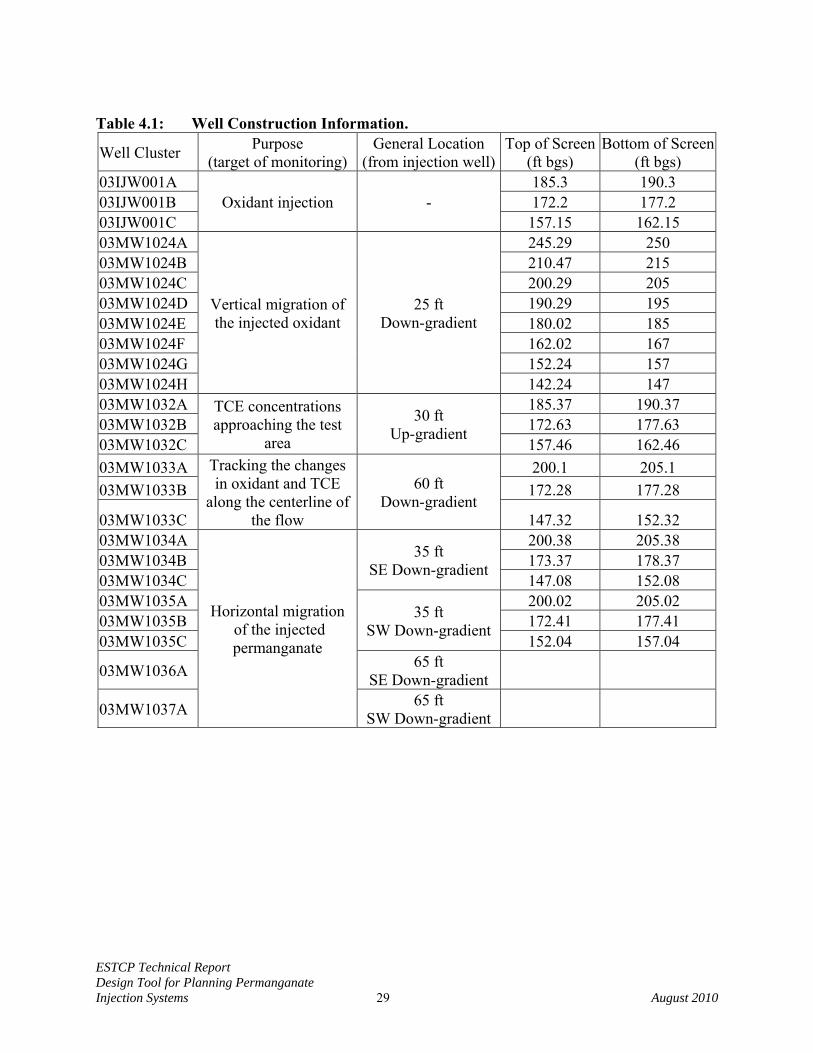
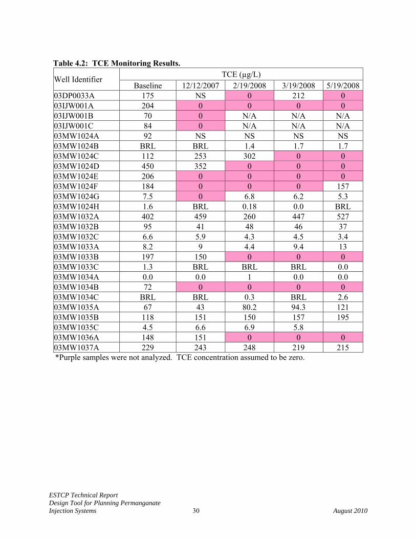
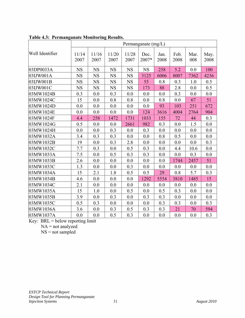
The pilot test area contained a single injection well and seven monitoring wells. The injection well (03IJW001) had three separate screened intervals allowing injection at different depths. The monitoring wells were installed up-gradient, cross-gradient, and down-gradient of the injection location with 22 well screens allowing monitoring at different depths. Table 4.1 provides details on the screened interval of each injection and monitoring well. The pilot test design consisted of injecting approximately 5,000 mg/L NaMnO4 for 10 hours per day for four days. This solution was to be injected into three injection wells simultaneously at 10 gallons per minute (gpm) for a total flow of 30 gpm. The plan was to inject a total volume of 72,000 gallons of water containing 1363 Kg NaMnO4. The actual injection flow rates and concentrations varied somewhat from this plan due to problems in maintaining a constant dilution rate and difficulty in maintaining high injection rates in the lower permeability zones. TCE and permanganate concentrations in the injection and selected monitor wells were measured five times between November 2007 and May 2008. Monitoring results are presented in Tables 4.2 and 4.3. Permanganate concentrations were determined by measuring manganese concentration in the water with a Hach Test Kit. TCE was not monitored when the groundwater had a purple color indicating the presence of dissolved permanganate. For model calibration purposes, the TCE concentration was assumed to be zero whenever dissolved permanganate was present as indicated by a purple color.
ESTCP Technical Report Design Tool for Planning Permanganate Injection Systems 29 August 2010
Table 4.1: Well Construction Information.
Well Cluster Purpose (target of monitoring)
General Location (from injection well)
Top of Screen (ft bgs)
Bottom of Screen(ft bgs)
03IJW001A Oxidant injection -
185.3 190.3 03IJW001B 172.2 177.2 03IJW001C 157.15 162.15 03MW1024A
Vertical migration of the injected oxidant
25 ft Down-gradient
245.29 250 03MW1024B 210.47 215 03MW1024C 200.29 205 03MW1024D 190.29 195 03MW1024E 180.02 185 03MW1024F 162.02 167 03MW1024G 152.24 157 03MW1024H 142.24 147 03MW1032A TCE concentrations
approaching the test area
30 ft Up-gradient
185.37 190.37 03MW1032B 172.63 177.63 03MW1032C 157.46 162.46 03MW1033A Tracking the changes
in oxidant and TCE along the centerline of
the flow
60 ft Down-gradient
200.1 205.1 03MW1033B 172.28 177.28
03MW1033C 147.32 152.32 03MW1034A
Horizontal migration of the injected permanganate
35 ft SE Down-gradient
200.38 205.38 03MW1034B 173.37 178.37 03MW1034C 147.08 152.08 03MW1035A
35 ft SW Down-gradient
200.02 205.02 03MW1035B 172.41 177.41 03MW1035C 152.04 157.04
03MW1036A 65 ft SE Down-gradient
03MW1037A 65 ft SW Down-gradient
ESTCP Technical Report Design Tool for Planning Permanganate Injection Systems 30 August 2010
Table 4.2: TCE Monitoring Results.
Well Identifier TCE (µg/L) Baseline 12/12/2007 2/19/2008 3/19/2008 5/19/2008
03DP0033A 175 NS 0 212 0 03IJW001A 204 0 0 0 0 03IJW001B 70 0 N/A N/A N/A 03IJW001C 84 0 N/A N/A N/A 03MW1024A 92 NS NS NS NS 03MW1024B BRL BRL 1.4 1.7 1.7 03MW1024C 112 253 302 0 0 03MW1024D 450 352 0 0 0 03MW1024E 206 0 0 0 0 03MW1024F 184 0 0 0 157 03MW1024G 7.5 0 6.8 6.2 5.3 03MW1024H 1.6 BRL 0.18 0.0 BRL 03MW1032A 402 459 260 447 527 03MW1032B 95 41 48 46 37 03MW1032C 6.6 5.9 4.3 4.5 3.4 03MW1033A 8.2 9 4.4 9.4 13 03MW1033B 197 150 0 0 0 03MW1033C 1.3 BRL BRL BRL 0.0 03MW1034A 0.0 0.0 1 0.0 0.0 03MW1034B 72 0 0 0 0 03MW1034C BRL BRL 0.3 BRL 2.6 03MW1035A 67 43 80.2 94.3 121 03MW1035B 118 151 150 157 195 03MW1035C 4.5 6.6 6.9 5.8 03MW1036A 148 151 0 0 0 03MW1037A 229 243 248 219 215 *Purple samples were not analyzed. TCE concentration assumed to be zero.
ESTCP Technical Report Design Tool for Planning Permanganate Injection Systems 31 August 2010
Table 4.3: Permanganate Monitoring Results.
Well Identifier
Permanganate (mg/L)
11/14 2007
11/162007
11/202007
11/282007
Dec.2007*
Jan. 2008
Feb. 2008
Mar.008
May.2008
03DP0033A NS NS NS NS NS 258 5.2 0.0 100 03IJW001A NS NS NS NS 3125 6006 8007 7362 4236 03IJW001B NS NS NS NS 55 0.8 0.3 1.0 0.5 03IJW001C NS NS NS NS 173 88 2.8 0.0 0.5 03MW1024B 0.3 0.0 0.3 0.0 0.0 0.0 0.3 0.0 0.0 03MW1024C 15 0.0 0.8 0.8 0.0 0.8 0.0 67 51 03MW1024D 0.0 0.0 0.0 0.0 0.0 93 103 251 672 03MW1024E 0.0 0.0 0.0 0.0 124 3616 4004 2764 904 03MW1024F 4.4 258 1472 1731 1033 155 72 44 0.3 03MW1024G 0.5 0.0 0.0 2661 982 0.3 0.0 1.5 0.0 03MW1024H 0.0 0.0 0.3 0.0 0.3 0.0 0.0 0.0 0.0 03MW1032A 3.4 0.3 0.3 0.0 0.0 0.8 0.5 0.0 0.0 03MW1032B 19 0.0 0.3 2.8 0.0 0.0 0.0 0.0 0.3 03MW1032C 7.7 0.3 0.0 0.5 0.3 0.0 4.4 10.6 0.0 03MW1033A 7.5 0.0 0.5 0.3 0.3 0.0 0.0 0.3 0.0 03MW1033B 2.6 0.0 0.0 0.0 0.0 0.0 1744 2457 51 03MW1033C 1.3 0.0 0.0 0.3 0.0 0.0 0.0 0.0 0.0 03MW1034A 15 2.1 1.8 0.5 0.5 29 0.8 5.7 0.3 03MW1034B 4.6 0.0 0.0 0.0 1292 5554 3810 1485 15 03MW1034C 2.1 0.0 0.0 0.0 0.0 0.0 0.0 0.0 0.0 03MW1035A 15 1.0 0.0 0.5 0.0 0.5 0.3 0.0 0.0 03MW1035B 3.9 0.0 0.3 0.0 0.3 0.3 0.0 0.0 0.0 03MW1035C 0.5 0.3 0.0 0.0 0.0 0.3 0.3 0.0 0.3 03MW1036A 3.6 0.0 0.3 0.5 0.3 0.3 21 70 594 03MW1037A 0.0 0.0 0.5 0.3 0.0 0.0 0.0 0.0 0.3 Key: BRL = below reporting limit
NA = not analyzed NS = not sampled
ESTCP Technical Report Design Tool for Planning Permanganate Injection Systems 32 August 2010
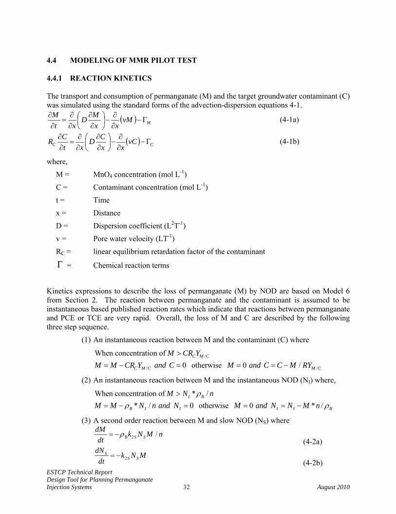
4.4 MODELING OF MMR PILOT TEST 4.4.1 REACTION KINETICS The transport and consumption of permanganate (M) and the target groundwater contaminant (C) was simulated using the standard forms of the advection-dispersion equations 4-1.
( ) MvMxx
MDxt
MΓ−
∂∂
−⎟⎠⎞
⎜⎝⎛
∂∂
∂∂
=∂∂ (4-1a)
( ) CC vCxx
CDxt
CR Γ−∂∂
−⎟⎠⎞
⎜⎝⎛
∂∂
∂∂
=∂∂ (4-1b)
where,
M = MnO4 concentration (mol L-1)
C = Contaminant concentration (mol L-1)
t = Time
x = Distance
D = Dispersion coefficient (L2T-1)
v = Pore water velocity (LT-1)
RC = linear equilibrium retardation factor of the contaminant
Γ = Chemical reaction terms
Kinetics expressions to describe the loss of permanganate (M) by NOD are based on Model 6 from Section 2. The reaction between permanganate and the contaminant is assumed to be instantaneous based published reaction rates which indicate that reactions between permanganate and PCE or TCE are very rapid. Overall, the loss of M and C are described by the following three step sequence.
(1) An instantaneous reaction between M and the contaminant (C) where
/
/ /
When concentration of 0 otherwise 0 /
C M C
C M C M C
M CR YM M CR Y and C M and C C M RY
>= − = = = −
(2) An instantaneous reaction between M and the instantaneous NOD (NI) where,
When concentration of * /* / 0 otherwise 0 * /
I B
B I I I I B
M N nM M N n and N M and N N M n
ρρ ρ
>= − = = = −
(3) A second order reaction between M and slow NOD (NS) where
2 /B S SdM k N M ndt
ρ= − (4-2a)
2S
S SdN k N Mdt
= − (4-2b)
ESTCP Technical Report Design Tool for Planning Permanganate Injection Systems 33 August 2010
and,
NI = Instantaneous NOD (mol Kg-1)
NS = Slow NOD (mol Kg-1)
ρB = bulk density (Kg L-1)
YM/C = molar ratio of M to C consumed (mol/mol)
k2S = 2nd order Slow NOD consumption rate (L mol-1 d-1)
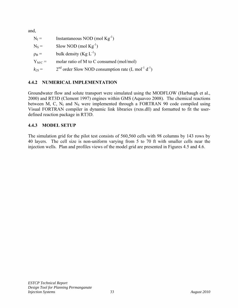
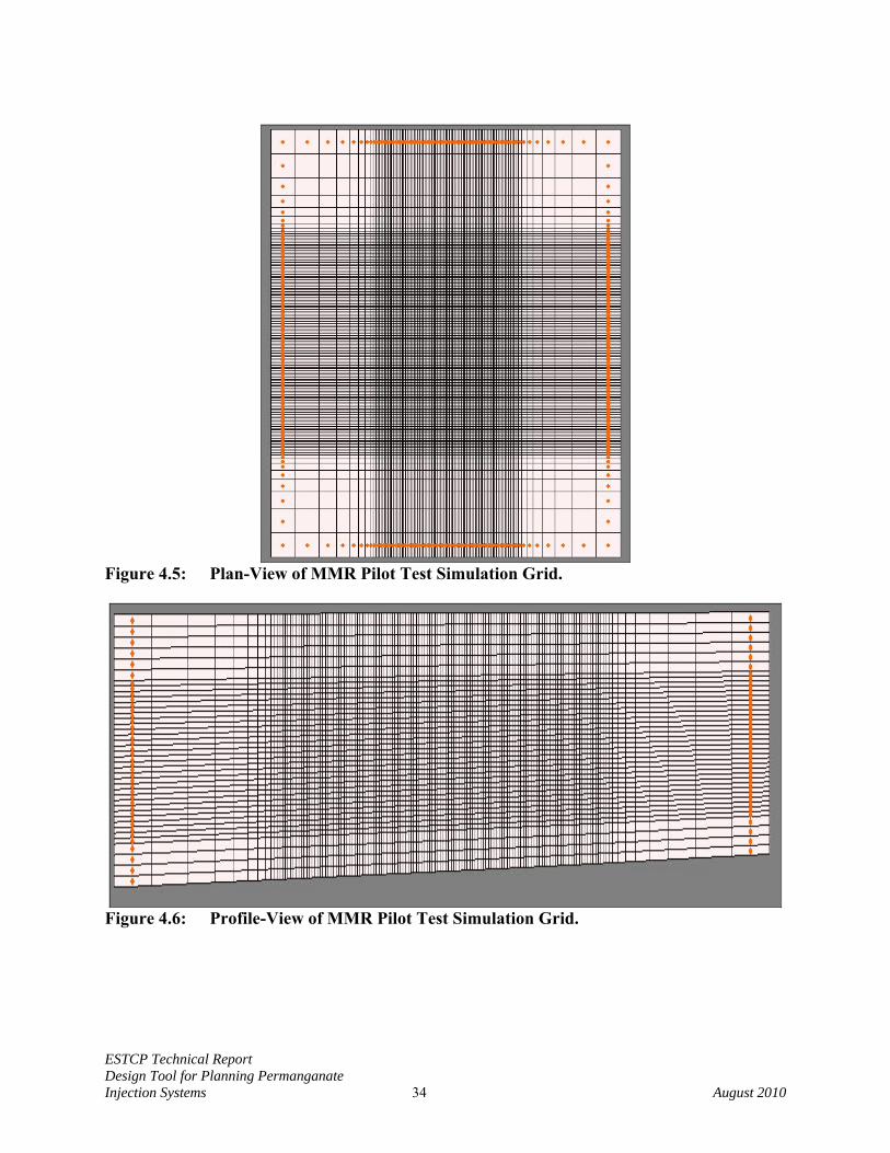
4.4.2 NUMERICAL IMPLEMENTATION Groundwater flow and solute transport were simulated using the MODFLOW (Harbaugh et al., 2000) and RT3D (Clement 1997) engines within GMS (Aquaveo 2008). The chemical reactions between M, C, NI and NS were implemented through a FORTRAN 90 code compiled using Visual FORTRAN compiler in dynamic link libraries (rxns.dll) and formatted to fit the user-defined reaction package in RT3D. 4.4.3 MODEL SETUP The simulation grid for the pilot test consists of 560,560 cells with 98 columns by 143 rows by 40 layers. The cell size is non-uniform varying from 5 to 70 ft with smaller cells near the injection wells. Plan and profiles views of the model grid are presented in Figures 4.5 and 4.6.
ESTCP Technical Report Design Tool for Planning Permanganate Injection Systems 34 August 2010
Figure 4.5: Plan-View of MMR Pilot Test Simulation Grid.
Figure 4.6: Profile-View of MMR Pilot Test Simulation Grid.
ESTCP Technical Report Design Tool for Planning Permanganate Injection Systems 35 August 2010
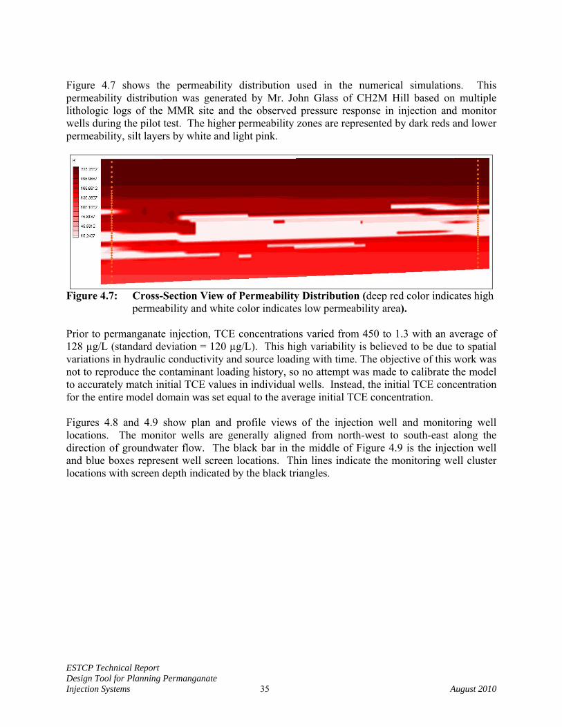
Figure 4.7 shows the permeability distribution used in the numerical simulations. This permeability distribution was generated by Mr. John Glass of CH2M Hill based on multiple lithologic logs of the MMR site and the observed pressure response in injection and monitor wells during the pilot test. The higher permeability zones are represented by dark reds and lower permeability, silt layers by white and light pink.
Figure 4.7: Cross-Section View of Permeability Distribution (deep red color indicates high
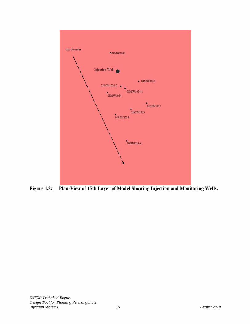
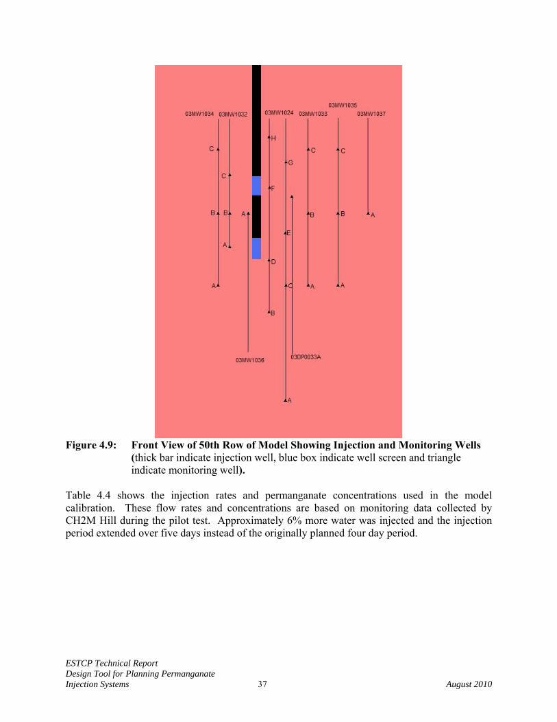
permeability and white color indicates low permeability area). Prior to permanganate injection, TCE concentrations varied from 450 to 1.3 with an average of 128 µg/L (standard deviation = 120 µg/L). This high variability is believed to be due to spatial variations in hydraulic conductivity and source loading with time. The objective of this work was not to reproduce the contaminant loading history, so no attempt was made to calibrate the model to accurately match initial TCE values in individual wells. Instead, the initial TCE concentration for the entire model domain was set equal to the average initial TCE concentration. Figures 4.8 and 4.9 show plan and profile views of the injection well and monitoring well locations. The monitor wells are generally aligned from north-west to south-east along the direction of groundwater flow. The black bar in the middle of Figure 4.9 is the injection well and blue boxes represent well screen locations. Thin lines indicate the monitoring well cluster locations with screen depth indicated by the black triangles.
ESTCP Technical Report Design Tool for Planning Permanganate Injection Systems 36 August 2010
Figure 4.8: Plan-View of 15th Layer of Model Showing Injection and Monitoring Wells.
ESTCP Technical Report Design Tool for Planning Permanganate Injection Systems 37 August 2010
Figure 4.9: Front View of 50th Row of Model Showing Injection and Monitoring Wells
(thick bar indicate injection well, blue box indicate well screen and triangle indicate monitoring well).
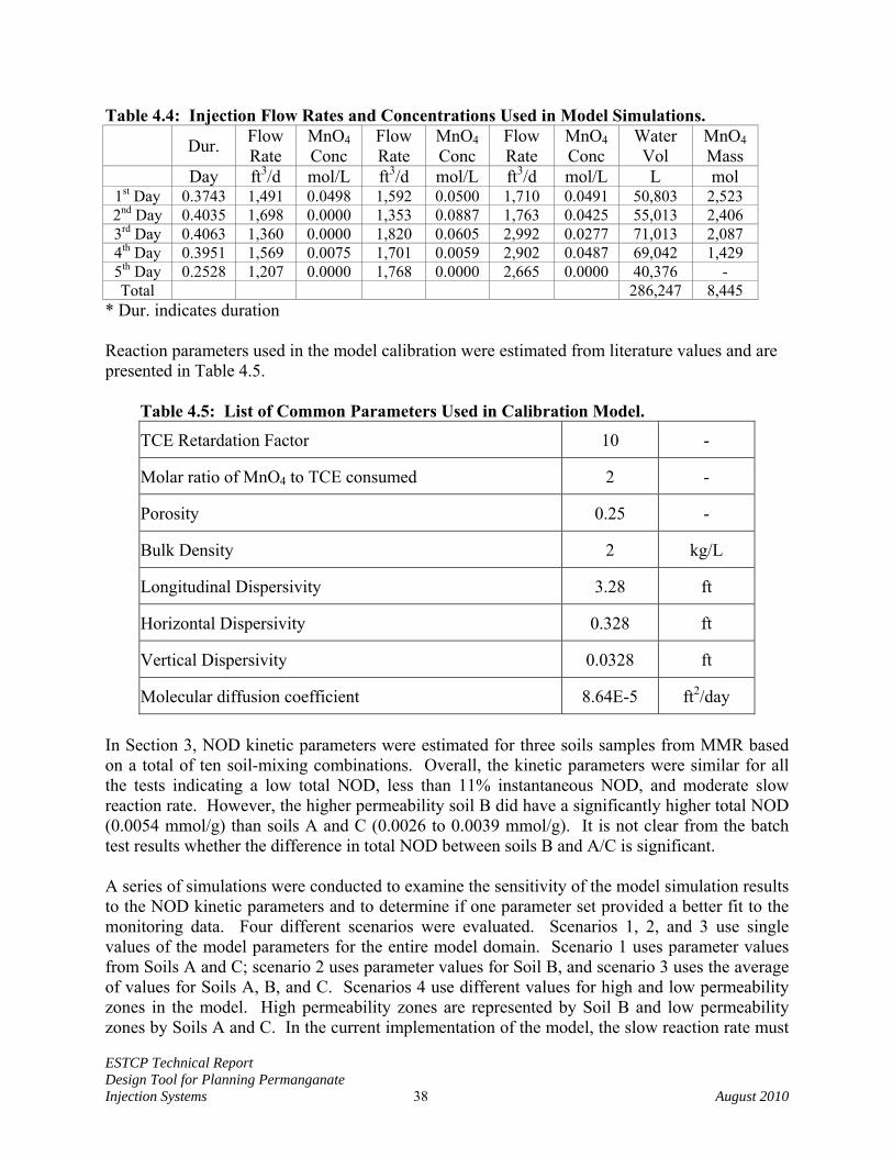
Table 4.4 shows the injection rates and permanganate concentrations used in the model calibration. These flow rates and concentrations are based on monitoring data collected by CH2M Hill during the pilot test. Approximately 6% more water was injected and the injection period extended over five days instead of the originally planned four day period.
ESTCP Technical Report Design Tool for Planning Permanganate Injection Systems 38 August 2010
Table 4.4: Injection Flow Rates and Concentrations Used in Model Simulations.
Dur. Flow Rate
MnO4 Conc
Flow Rate
MnO4 Conc
Flow Rate
MnO4 Conc
Water Vol
MnO4 Mass
Day ft3/d mol/L ft3/d mol/L ft3/d mol/L L mol 1st Day 0.3743 1,491 0.0498 1,592 0.0500 1,710 0.0491 50,803 2,523 2nd Day 0.4035 1,698 0.0000 1,353 0.0887 1,763 0.0425 55,013 2,406 3rd Day 0.4063 1,360 0.0000 1,820 0.0605 2,992 0.0277 71,013 2,087 4th Day 0.3951 1,569 0.0075 1,701 0.0059 2,902 0.0487 69,042 1,429 5th Day 0.2528 1,207 0.0000 1,768 0.0000 2,665 0.0000 40,376 - Total 286,247 8,445
* Dur. indicates duration Reaction parameters used in the model calibration were estimated from literature values and are presented in Table 4.5. Table 4.5: List of Common Parameters Used in Calibration Model.
TCE Retardation Factor 10 -
Molar ratio of MnO4 to TCE consumed 2 -
Porosity 0.25 -
Bulk Density 2 kg/L
Longitudinal Dispersivity 3.28 ft
Horizontal Dispersivity 0.328 ft
Vertical Dispersivity 0.0328 ft
Molecular diffusion coefficient 8.64E-5 ft2/day In Section 3, NOD kinetic parameters were estimated for three soils samples from MMR based on a total of ten soil-mixing combinations. Overall, the kinetic parameters were similar for all the tests indicating a low total NOD, less than 11% instantaneous NOD, and moderate slow reaction rate. However, the higher permeability soil B did have a significantly higher total NOD (0.0054 mmol/g) than soils A and C (0.0026 to 0.0039 mmol/g). It is not clear from the batch test results whether the difference in total NOD between soils B and A/C is significant. A series of simulations were conducted to examine the sensitivity of the model simulation results to the NOD kinetic parameters and to determine if one parameter set provided a better fit to the monitoring data. Four different scenarios were evaluated. Scenarios 1, 2, and 3 use single values of the model parameters for the entire model domain. Scenario 1 uses parameter values from Soils A and C; scenario 2 uses parameter values for Soil B, and scenario 3 uses the average of values for Soils A, B, and C. Scenarios 4 use different values for high and low permeability zones in the model. High permeability zones are represented by Soil B and low permeability zones by Soils A and C. In the current implementation of the model, the slow reaction rate must

ESTCP Technical Report Design Tool for Planning Permanganate Injection Systems 39 August 2010
be spatially uniform. Scenario 4 uses the averaged slow reaction rate for Soils A, B, and C. Table 4.6 presents the values of each parameter used in the simulations. Table 4.6: Details of 4 Simulation Scenarios
Scenario Soil Type
Fraction Instantaneous
Instantaneous NOD
Slow NOD
Slow Reaction Rate
mmol/g mmol/g L/mmol-d 1 A,C 0.09 0.0003 0.0028 0.0051 2 B 0.06 0.0003 0.0051 0.0163 3 A,B,C 0.08 0.0003 0.0035 0.0089
4 B 0.06 0.0003 0.0051
0.0107 A,C 0.09 0.0003 0.0028
4.5 MODEL CALIBRATION The pilot test was simulating using four different sets of NOD kinetic parameter (see Table 4.6). The goodness of fit was evaluated by comparing the simulated and observed permanganate and TCE distributions at various time points. Two different error statistics were used: (1) root mean squared error; and (2) a qualitative statistic indicating the presence or absence of a compound at each monitoring point. 4.5.1 SIMPLE SCORING ERROR STATISTICS (SSES) Permanganate reacts very rapidly with TCE. As a consequence, if permanganate reaches a zone, TCE is rapidly reduced to zero. Under these conditions, the presence or absence of permanganate in a monitoring well is often a more important indicator of treatment, than the absolute concentration of permanganate or TCE concentration observed in that well. To provide a more appropriate representation of this condition, the simple scoring error statistic (SSES) was developed. Using the SSES procedure, a monitor well is considered ‘contacted’ if the concentration of a solute (MnO4 or TCE) is greater than 0.1% of the maximum concentration observed at the site. Each monitor well is then evaluated to determine if the model accurately matched the field observations. For example, if both the field and monitoring data indicate that MnO4 is present in one well during a single sampling event, that is counted as ‘matched’. Conversely, if the model indicates TCE is present (at over 0.1% of max. conc.) and the field data indicate TCE is below detection that observation is a ‘not matched’. The fractions of matched observations are then reported for both TCE and MnO4.
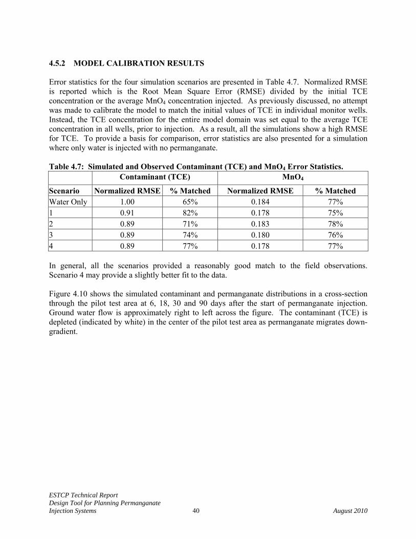
ESTCP Technical Report Design Tool for Planning Permanganate Injection Systems 40 August 2010
4.5.2 MODEL CALIBRATION RESULTS Error statistics for the four simulation scenarios are presented in Table 4.7. Normalized RMSE is reported which is the Root Mean Square Error (RMSE) divided by the initial TCE concentration or the average MnO4 concentration injected. As previously discussed, no attempt was made to calibrate the model to match the initial values of TCE in individual monitor wells. Instead, the TCE concentration for the entire model domain was set equal to the average TCE concentration in all wells, prior to injection. As a result, all the simulations show a high RMSE for TCE. To provide a basis for comparison, error statistics are also presented for a simulation where only water is injected with no permanganate. Table 4.7: Simulated and Observed Contaminant (TCE) and MnO4 Error Statistics. Contaminant (TCE) MnO4
Scenario Normalized RMSE % Matched Normalized RMSE % Matched Water Only 1.00 65% 0.184 77% 1 0.91 82% 0.178 75% 2 0.89 71% 0.183 78% 3 0.89 74% 0.180 76% 4 0.89 77% 0.178 77% In general, all the scenarios provided a reasonably good match to the field observations. Scenario 4 may provide a slightly better fit to the data. Figure 4.10 shows the simulated contaminant and permanganate distributions in a cross-section through the pilot test area at 6, 18, 30 and 90 days after the start of permanganate injection. Ground water flow is approximately right to left across the figure. The contaminant (TCE) is depleted (indicated by white) in the center of the pilot test area as permanganate migrates down-gradient.
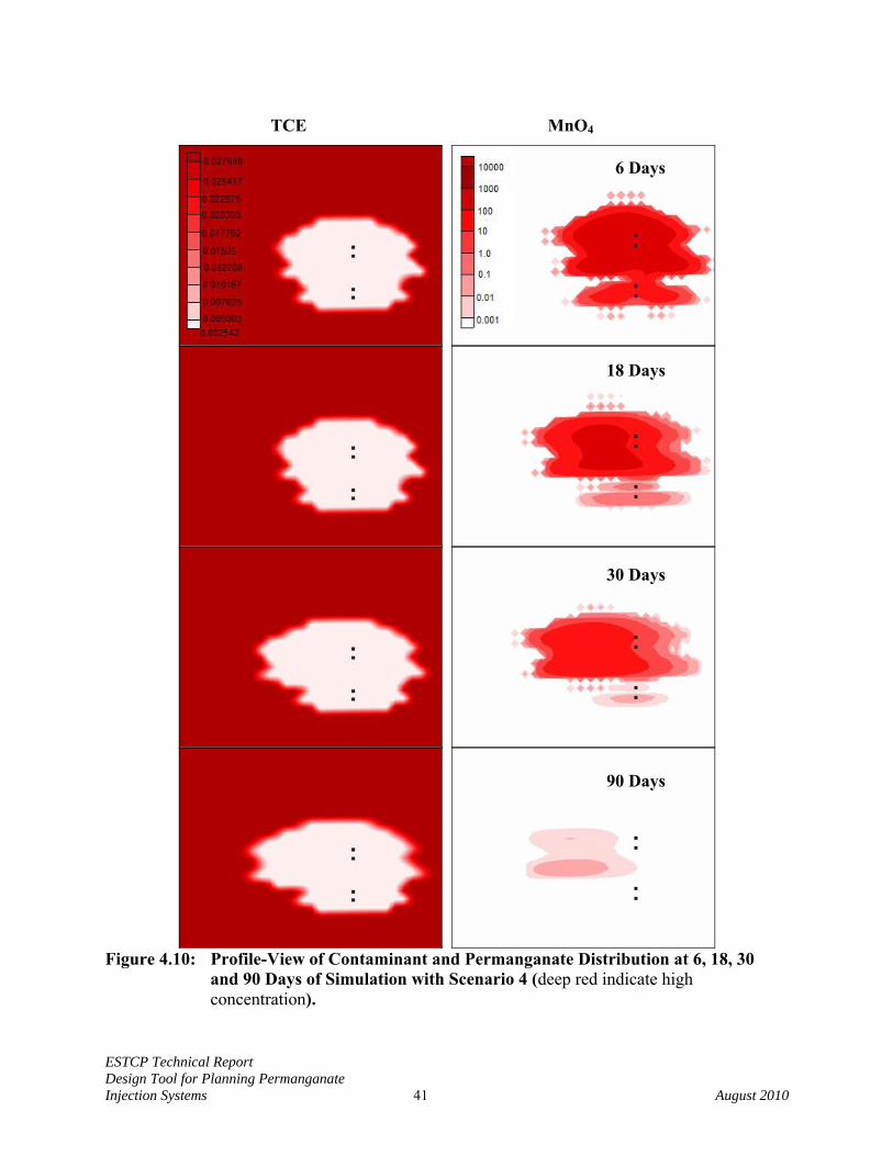
ESTCP Technical Report Design Tool for Planning Permanganate Injection Systems 41 August 2010
Figure 4.10: Profile-View of Contaminant and Permanganate Distribution at 6, 18, 30
and 90 Days of Simulation with Scenario 4 (deep red indicate high concentration).
30 Days
90 Days
18 Days
6 Days
TCE MnO4
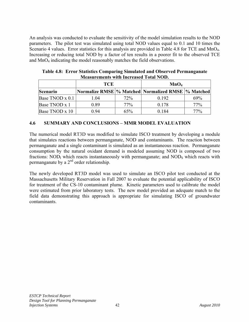
ESTCP Technical Report Design Tool for Planning Permanganate Injection Systems 42 August 2010
An analysis was conducted to evaluate the sensitivity of the model simulation results to the NOD parameters. The pilot test was simulated using total NOD values equal to 0.1 and 10 times the Scenario 4 values. Error statistics for this analysis are provided in Table 4.8 for TCE and MnO4. Increasing or reducing total NOD by a factor of ten results in a poorer fit to the observed TCE and MnO4 indicating the model reasonably matches the field observations.
Table 4.8: Error Statistics Comparing Simulated and Observed Permanganate Measurements with Increased Total NOD.
TCE MnO4 Scenario Normalize RMSE % Matched Normalized RMSE % MatchedBase TNOD x 0.1 1.04 72% 0.192 69% Base TNOD x 1 0.89 77% 0.178 77% Base TNOD x 10 0.94 65% 0.184 77%
4.6 SUMMARY AND CONCLUSIONS – MMR MODEL EVALUATION The numerical model RT3D was modified to simulate ISCO treatment by developing a module that simulates reactions between permanganate, NOD and contaminants. The reaction between permanganate and a single contaminant is simulated as an instantaneous reaction. Permanganate consumption by the natural oxidant demand is modeled assuming NOD is composed of two fractions: NODI which reacts instantaneously with permanganate; and NODS which reacts with permanganate by a 2nd order relationship. The newly developed RT3D model was used to simulate an ISCO pilot test conducted at the Massachusetts Military Reservation in Fall 2007 to evaluate the potential applicability of ISCO for treatment of the CS-10 contaminant plume. Kinetic parameters used to calibrate the model were estimated from prior laboratory tests. The new model provided an adequate match to the field data demonstrating this approach is appropriate for simulating ISCO of groundwater contaminants.
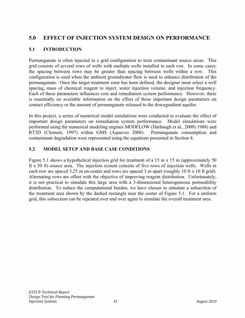
ESTCP Technical Report Design Tool for Planning Permanganate Injection Systems 43 August 2010
5.0 EFFECT OF INJECTION SYSTEM DESIGN ON PERFORMANCE 5.1 INTRODUCTION Permanganate is often injected in a grid configuration to treat contaminant source areas. This grid consists of several rows of wells with multiple wells installed in each row. In some cases, the spacing between rows may be greater than spacing between wells within a row. This configuration is used when the ambient groundwater flow is used to enhance distribution of the permanganate. Once the target treatment zone has been defined, the designer must select a well spacing, mass of chemical reagent to inject, water injection volume, and injection frequency. Each of these parameters influences cost and remediation system performance. However, there is essentially no available information on the effect of these important design parameters on contact efficiency or the amount of permanganate released to the downgradient aquifer. In this project, a series of numerical model simulations were conducted to evaluate the effect of important design parameters on remediation system performance. Model simulations were performed using the numerical modeling engines MODFLOW (Harbaugh et al., 2000) 1988) and RT3D (Clement, 1997) within GMS (Aquaveo 2008). Permanganate consumption and contaminant degradation were represented using the equations presented in Section 4. 5.2 MODEL SETUP AND BASE CASE CONDITIONS Figure 5.1 shows a hypothetical injection grid for treatment of a 15 m x 15 m (approximately 50 ft x 50 ft) source area. The injection system consists of five rows of injection wells. Wells in each row are spaced 3.25 m on-center and rows are spaced 3 m apart (roughly 10 ft x 10 ft grid). Alternating rows are offset with the objective of improving reagent distribution. Unfortunately, it is not practical to simulate this large area with a 3-dimensional heterogeneous permeability distribution. To reduce the computational burden, we have chosen to simulate a subsection of the treatment area shown by the dashed rectangle near the center of Figure 5.1. For a uniform grid, this subsection can be repeated over and over again to simulate the overall treatment area.
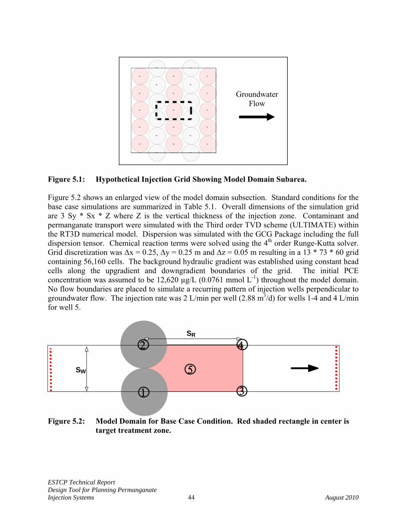
ESTCP Technical Report Design Tool for Planning Permanganate Injection Systems 44 August 2010
Figure 5.1: Hypothetical Injection Grid Showing Model Domain Subarea. Figure 5.2 shows an enlarged view of the model domain subsection. Standard conditions for the base case simulations are summarized in Table 5.1. Overall dimensions of the simulation grid are 3 Sy * Sx * Z where Z is the vertical thickness of the injection zone. Contaminant and permanganate transport were simulated with the Third order TVD scheme (ULTIMATE) within the RT3D numerical model. Dispersion was simulated with the GCG Package including the full dispersion tensor. Chemical reaction terms were solved using the 4th order Runge-Kutta solver. Grid discretization was Δx = 0.25, Δy = 0.25 m and Δz = 0.05 m resulting in a 13 * 73 * 60 grid containing 56,160 cells. The background hydraulic gradient was established using constant head cells along the upgradient and downgradient boundaries of the grid. The initial PCE concentration was assumed to be 12,620 µg/L (0.0761 mmol L-1) throughout the model domain. No flow boundaries are placed to simulate a recurring pattern of injection wells perpendicular to groundwater flow. The injection rate was 2 L/min per well (2.88 m3/d) for wells 1-4 and 4 L/min for well 5.
SR
SW
1
5
2
3
4
Figure 5.2: Model Domain for Base Case Condition. Red shaded rectangle in center is
target treatment zone.
Groundwater Flow
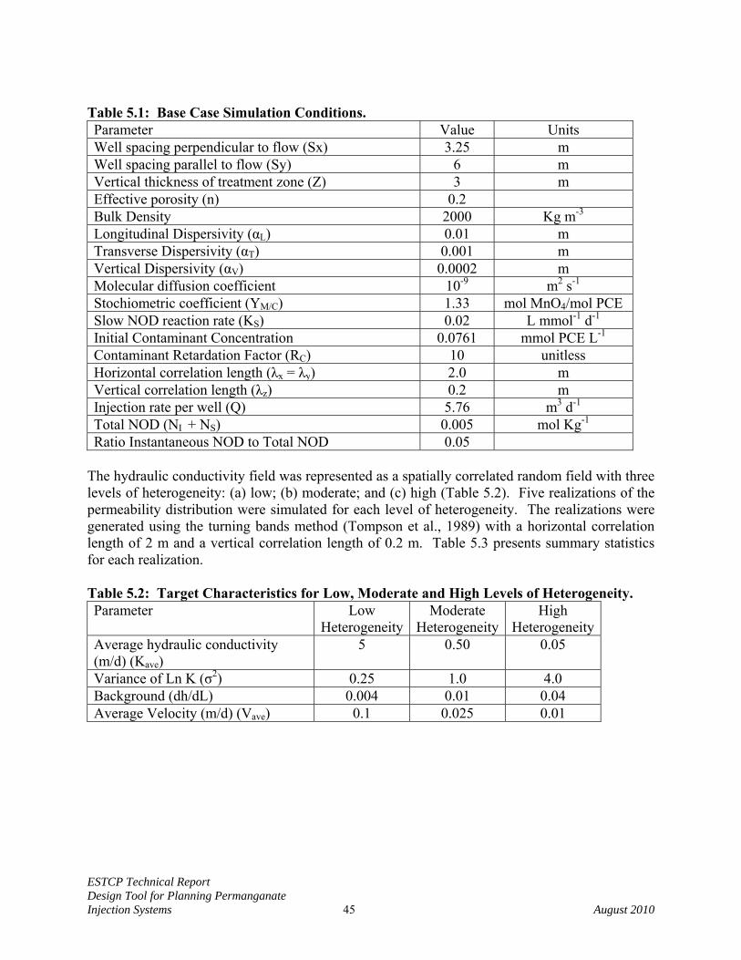
ESTCP Technical Report Design Tool for Planning Permanganate Injection Systems 45 August 2010
Table 5.1: Base Case Simulation Conditions. Parameter Value Units Well spacing perpendicular to flow (Sx) 3.25 m Well spacing parallel to flow (Sy) 6 m Vertical thickness of treatment zone (Z) 3 m Effective porosity (n) 0.2 Bulk Density 2000 Kg m-3 Longitudinal Dispersivity (αL) 0.01 m Transverse Dispersivity (αT) 0.001 m Vertical Dispersivity (αV) 0.0002 m Molecular diffusion coefficient 10-9 m2 s-1 Stochiometric coefficient (YM/C) 1.33 mol MnO4/mol PCE Slow NOD reaction rate (KS) 0.02 L mmol-1 d-1 Initial Contaminant Concentration 0.0761 mmol PCE L-1 Contaminant Retardation Factor (RC) 10 unitless Horizontal correlation length (λx = λy) 2.0 m Vertical correlation length (λz) 0.2 m Injection rate per well (Q) 5.76 m3 d-1 Total NOD (NI + NS) 0.005 mol Kg-1 Ratio Instantaneous NOD to Total NOD 0.05
The hydraulic conductivity field was represented as a spatially correlated random field with three levels of heterogeneity: (a) low; (b) moderate; and (c) high (Table 5.2). Five realizations of the permeability distribution were simulated for each level of heterogeneity. The realizations were generated using the turning bands method (Tompson et al., 1989) with a horizontal correlation length of 2 m and a vertical correlation length of 0.2 m. Table 5.3 presents summary statistics for each realization. Table 5.2: Target Characteristics for Low, Moderate and High Levels of Heterogeneity. Parameter Low
HeterogeneityModerate
HeterogeneityHigh
Heterogeneity Average hydraulic conductivity (m/d) (Kave)
5 0.50 0.05
Variance of Ln K (σ2) 0.25 1.0 4.0 Background (dh/dL) 0.004 0.01 0.04 Average Velocity (m/d) (Vave) 0.1 0.025 0.01
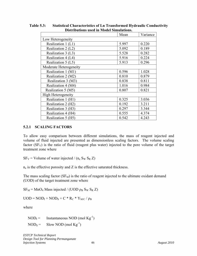
ESTCP Technical Report Design Tool for Planning Permanganate Injection Systems 46 August 2010
Table 5.3: Statistical Characteristics of Ln Transformed Hydraulic Conductivity Distributions used in Model Simulations.
Mean Variance Low Heterogeneity Realization 1 (L1) 5.997 0.220 Realization 2 (L2) 5.092 0.189 Realization 3 (L3) 5.528 0.282 Realization 4 (L4) 5.916 0.224 Realization 5 (L5) 5.913 0.296 Moderate Heterogeneity Realization 1 (M1) 0.596 1.028 Realization 2 (M2) 0.810 0.879 Realization 3 (M3) 0.838 0.811 Realization 4 (M4) 1.016 0.984 Realization 5 (M5) 0.807 0.821 High Heterogeneity Realization 1 (H1) 0.325 3.036 Realization 2 (H2) 0.192 3.211 Realization 3 (H3) 0.297 3.344 Realization 4 (H4) 0.555 4.374 Realization 5 (H5) 0.542 4.243
5.2.1 SCALING FACTORS To allow easy comparison between different simulations, the mass of reagent injected and volume of fluid injected are presented as dimensionless scaling factors. The volume scaling factor (SFV) is the ratio of fluid (reagent plus water) injected to the pore volume of the target treatment zone where SFV = Volume of water injected / (ne SW SR Z) ne is the effective porosity and Z is the effective saturated thickness. The mass scaling factor (SFM) is the ratio of reagent injected to the ultimate oxidant demand (UOD) of the target treatment zone where SFM = MnO4 Mass injected / (UOD ρB SW SR Z) UOD = NODI + NODS + C * RC * YM/C / ρB where
NODI = Instantaneous NOD (mol Kg-1)
NODS = Slow NOD (mol Kg-1)
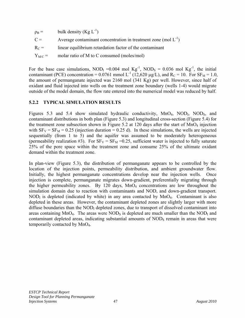
ESTCP Technical Report Design Tool for Planning Permanganate Injection Systems 47 August 2010
ρB = bulk density (Kg L-1)
C = Average contaminant concentration in treatment zone (mol L-1)
RC = linear equilibrium retardation factor of the contaminant
YM/C = molar ratio of M to C consumed (moles/mol)
For the base case simulations, NODI =0.004 mol Kg-1, NODS = 0.036 mol Kg-1, the initial contaminant (PCE) concentration = 0.0761 mmol L-1 (12,620 µg/L), and RC = 10. For SFM = 1.0, the amount of permanganate injected was 2160 mol (341 Kg) per well. However, since half of oxidant and fluid injected into wells on the treatment zone boundary (wells 1-4) would migrate outside of the model domain, the flow rate entered into the numerical model was reduced by half. 5.2.2 TYPICAL SIMULATION RESULTS Figures 5.3 and 5.4 show simulated hydraulic conductivity, MnO4, NODI, NODS, and contaminant distributions in both plan (Figure 5.3) and longitudinal cross-section (Figure 5.4) for the treatment zone subsection shown in Figure 5.2 at 120 days after the start of MnO4 injection with SFV = SFM = 0.25 (injection duration = 0.25 d). In these simulations, the wells are injected sequentially (from 1 to 5) and the aquifer was assumed to be moderately heterogeneous (permeability realization #3). For SFV = SFM =0.25, sufficient water is injected to fully saturate 25% of the pore space within the treatment zone and consume 25% of the ultimate oxidant demand within the treatment zone. In plan-view (Figure 5.3), the distribution of permanganate appears to be controlled by the location of the injection points, permeability distribution, and ambient groundwater flow. Initially, the highest permanganate concentrations develop near the injection wells. Once injection is complete, permanganate migrates down-gradient, preferentially migrating through the higher permeability zones. By 120 days, MnO4 concentrations are low throughout the simulation domain due to reaction with contaminants and NOD, and down-gradient transport. NODI is depleted (indicated by white) in any area contacted by MnO4. Contaminant is also depleted in these areas. However, the contaminant depleted zones are slightly larger with more diffuse boundaries than the NODI depleted zones, due to transport of dissolved contaminant into areas containing MnO4. The areas were NODS is depleted are much smaller than the NODI and contaminant depleted areas, indicating substantial amounts of NODS remain in areas that were temporarily contacted by MnO4.
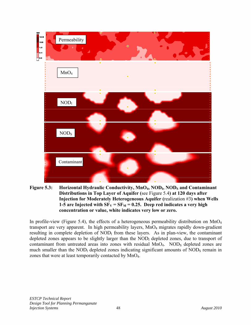
ESTCP Technical Report Design Tool for Planning Permanganate Injection Systems 48 August 2010
Figure 5.3: Horizontal Hydraulic Conductivity, MnO4, NODI, NODS and Contaminant
Distributions in Top Layer of Aquifer (see Figure 5.4) at 120 days after Injection for Moderately Heterogeneous Aquifer (realization #3) when Wells 1-5 are Injected with SFV = SFM = 0.25. Deep red indicates a very high concentration or value, white indicates very low or zero.
In profile-view (Figure 5.4), the effects of a heterogeneous permeability distribution on MnO4 transport are very apparent. In high permeability layers, MnO4 migrates rapidly down-gradient resulting in complete depletion of NODI from these layers. As in plan-view, the contaminant depleted zones appears to be slightly larger than the NODI depleted zones, due to transport of contaminant from untreated areas into zones with residual MnO4. NODS depleted zones are much smaller than the NODI depleted zones indicating significant amounts of NODS remain in zones that were at least temporarily contacted by MnO4.
Permeability
MnO4
NODS
Contaminant
NODI
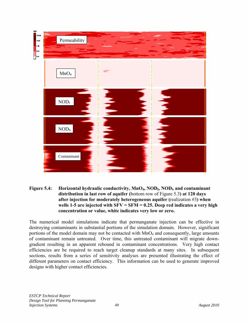
ESTCP Technical Report Design Tool for Planning Permanganate Injection Systems 49 August 2010
Figure 5.4: Horizontal hydraulic conductivity, MnO4, NODI, NODS and contaminant
distribution in last row of aquifer (bottom row of Figure 5.3) at 120 days after injection for moderately heterogeneous aquifer (realization #3) when wells 1-5 are injected with SFV = SFM = 0.25. Deep red indicates a very high concentration or value, white indicates very low or zero.
The numerical model simulations indicate that permanganate injection can be effective in destroying contaminants in substantial portions of the simulation domain. However, significant portions of the model domain may not be contacted with MnO4 and consequently, large amounts of contaminant remain untreated. Over time, this untreated contaminant will migrate down-gradient resulting in an apparent rebound in contaminant concentrations. Very high contact efficiencies are be required to reach target cleanup standards at many sites. In subsequent sections, results from a series of sensitivity analyses are presented illustrating the effect of different parameters on contact efficiency. This information can be used to generate improved designs with higher contact efficiencies.
Permeability
MnO4
NODS
Contaminant
NODI
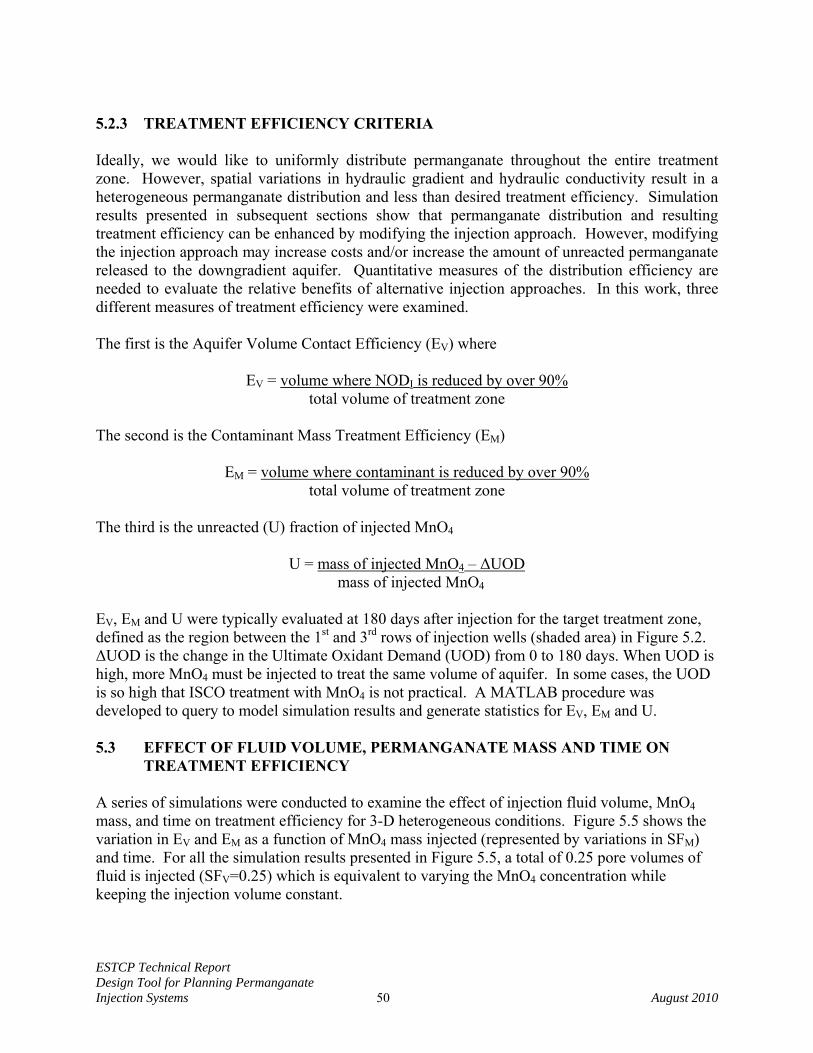
ESTCP Technical Report Design Tool for Planning Permanganate Injection Systems 50 August 2010
5.2.3 TREATMENT EFFICIENCY CRITERIA Ideally, we would like to uniformly distribute permanganate throughout the entire treatment zone. However, spatial variations in hydraulic gradient and hydraulic conductivity result in a heterogeneous permanganate distribution and less than desired treatment efficiency. Simulation results presented in subsequent sections show that permanganate distribution and resulting treatment efficiency can be enhanced by modifying the injection approach. However, modifying the injection approach may increase costs and/or increase the amount of unreacted permanganate released to the downgradient aquifer. Quantitative measures of the distribution efficiency are needed to evaluate the relative benefits of alternative injection approaches. In this work, three different measures of treatment efficiency were examined. The first is the Aquifer Volume Contact Efficiency (EV) where
EV = volume where NODI is reduced by over 90%
total volume of treatment zone The second is the Contaminant Mass Treatment Efficiency (EM)
EM = volume where contaminant is reduced by over 90%
total volume of treatment zone The third is the unreacted (U) fraction of injected MnO4
U = mass of injected MnO4 – ΔUOD
mass of injected MnO4 EV, EM and U were typically evaluated at 180 days after injection for the target treatment zone, defined as the region between the 1st and 3rd rows of injection wells (shaded area) in Figure 5.2. ΔUOD is the change in the Ultimate Oxidant Demand (UOD) from 0 to 180 days. When UOD is high, more MnO4 must be injected to treat the same volume of aquifer. In some cases, the UOD is so high that ISCO treatment with MnO4 is not practical. A MATLAB procedure was developed to query to model simulation results and generate statistics for EV, EM and U. 5.3 EFFECT OF FLUID VOLUME, PERMANGANATE MASS AND TIME ON
TREATMENT EFFICIENCY A series of simulations were conducted to examine the effect of injection fluid volume, MnO4 mass, and time on treatment efficiency for 3-D heterogeneous conditions. Figure 5.5 shows the variation in EV and EM as a function of MnO4 mass injected (represented by variations in SFM) and time. For all the simulation results presented in Figure 5.5, a total of 0.25 pore volumes of fluid is injected (SFV=0.25) which is equivalent to varying the MnO4 concentration while keeping the injection volume constant.
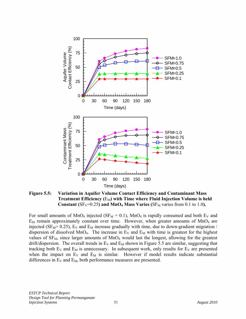
ESTCP Technical Report Design Tool for Planning Permanganate Injection Systems 51 August 2010
0 30 60 90 120 150 180Time (days)
0
25
50
75
100
Aqu
ifer V
olum
e C
onta
ct E
ffici
ency
(%)
SFM=1.0SFM=0.75SFM=0.5SFM=0.25SFM=0.1
0 30 60 90 120 150 180Time (days)
0
25
50
75
100
Con
tam
inan
t Mas
s Tr
eatm
ent E
ffici
ency
(%)
SFM=1.0SFM=0.75SFM=0.5SFM=0.25SFM=0.1
Figure 5.5: Variation in Aquifer Volume Contact Efficiency and Contaminant Mass
Treatment Efficiency (EM) with Time where Fluid Injection Volume is held Constant (SFV=0.25) and MnO4 Mass Varies (SFM varies from 0.1 to 1.0).
For small amounts of MnO4 injected (SFM = 0.1), MnO4 is rapidly consumed and both EV and EM remain approximately constant over time. However, when greater amounts of MnO4 are injected (SFM> 0.25), EV and EM increase gradually with time, due to down-gradient migration / dispersion of dissolved MnO4. The increase in EV and EM with time is greatest for the highest values of SFM, since larger amounts of MnO4 would last the longest, allowing for the greatest drift/dispersion. The overall trends in EV and EM shown in Figure 5.5 are similar, suggesting that tracking both EV and EM is unnecessary. In subsequent work, only results for EV are presented when the impact on EV and EM is similar. However if model results indicate substantial differences in EV and EM, both performance measures are presented.
ESTCP Technical Report Design Tool for Planning Permanganate Injection Systems 52 August 2010
Figure 5.6 shows the effect of varying MnO4 mass (varying SFM) and varying fluid volume (varying SFV) on EV and U at 180 days. For relatively small amounts of MnO4 injected (constant SFM = 0.1 to 0.25), increasing fluid volume injected (increasing SFV) results in a substantial improvement in EV. However, it also results in a substantial increase in the amount of MnO4 flushed out of the target treatment zone (indicated by increasing fraction unreacted MnO4). For larger amounts of MnO4 injected (SFM = 0.5 to 0.75), injecting large amounts of water provides less benefit in terms of improved contact efficiency (EV), but also less negative impacts associated with migration of MnO4 out of the target treatment zone.
0 0.25 0.5 0.75 1Volume Scaling Factor (SFV)
0
25
50
75
100
Aqu
ifer V
olum
e C
onta
ct E
ffici
ency
(%)
SFM=1.00SFM=0.75SFM=0.50SFM=0.25SFM=0.10
0 0.25 0.5 0.75 1Mass Scaling Factor (SFM)
0
25
50
75
100
Aqu
ifer V
olum
e C
onta
ct E
ffici
ency
(%)
SFV=1.00SFV=0.75SFV=0.50SFV=0.25SFV=0.10
0 0.25 0.5 0.75 1Volume Scaling Factor (SFV)
0
10
20
30
40
50
Unr
eact
ed M
nO4
(%)
SFM=0.10SFM=0.25SFM=0.50SFM=0.75SFM=1.00
0 0.25 0.5 0.75 1Mass Scaling Factor (SFM)
0
10
20
30
40
50
Unr
eact
ed M
nO4
(%)
SFV=0.10SFV=0.25SFV=0.50SFV=0.75SFV=1.00
Figure 5.6: Variation in Aquifer Volume Contact Efficiency (EV) and Fraction
Unreacted MnO4 (U) at 180 days after Injection with Mass and Volume Scaling Factors.
ESTCP Technical Report Design Tool for Planning Permanganate Injection Systems 53 August 2010
For relatively small injection volumes (SFV = 0.1 to 0.25), increasing MnO4 mass injected (increasing SFM) results in a substantial increase in EV and U. This trend is due to down-gradient drift/dispersion of MnO4 when larger amounts of reagent are injected. The highest volume contact (EV) occurs when both SFV and SFM are increased, but also results in the release of MnO4 outside of the target treatment zone (U). Injecting larger amounts of water (increasing SFV) result in more rapid distribution of the MnO4 before it is consumed by reaction with NODS. Injecting more MnO4 (increasing SFM) allows the MnO4 to last longer, contacting a greater portion of the aquifer. Overall, treatment efficiency appears to be best when SFM = SFV. This approach was used in subsequent analyses examining the effect of different parameters on EV. 5.4 EFFECT OF INJECTION DESIGN PARAMETERS ON PERFORMANCE The simulation results presented above demonstrate that increasing injection fluid volume and mass of MnO4 increases contact and treatment efficiency. Injection well spacing and reinjection frequency can also be adjusted to improve efficiency. Figure 5.7 shows the effects of varying the injection well spacing on EV and U at 180 days when the well spacing in a row is 3.25 m or 6.25 m, and the spacing between rows of injection wells is 3, 6, 9, or 12 m. In these simulations, the amount of solution injected per well is varied so that the total volume of fluid and mass of MnO4 injected per volume of treatment zone (SFV and SFM) remained constant for different well and row spacings. For both 3.25 and 6.25 m well spacing, increasing the row spacing had a modest impact on volume contact efficiency (EV) and fraction unreacted MnO4 (U) when SFV=SFM was less than 0.25. However for larger values of SFV=SFM (>0.5), increasing the row spacing had a substantial negative impact, reducing volume contact efficiency and increasing the amount of unreacted MnO4 released downgradient.
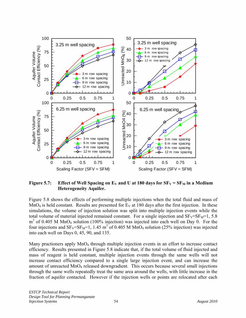
ESTCP Technical Report Design Tool for Planning Permanganate Injection Systems 54 August 2010
0 0.25 0.5 0.75 10
25
50
75
100A
quife
r Vol
ume
Con
tact
Effi
cien
cy (%
)
3 m row spacing6 m row spacing9 m row spacing12 m row spacing
3.25 m well spacing
0 0.25 0.5 0.75 1Scaling Factor (SFV = SFM)
0
25
50
75
100
Aqui
fer V
olum
eC
onta
ct E
ffici
ency
(%)
3 m row spacing6 m row spacing9 m row spacing12 m row spacing
6.25 m well spacing
0 0.25 0.5 0.75 10
10
20
30
40
50
Unr
eact
ed M
nO4
(%) 3 m row spacing
6 m row spacing9 m row spacing12 m row spacing
3.25 m well spacing
0 0.25 0.5 0.75 1Scaling Factor (SFV = SFM)
0
10
20
30
40
50
Unr
eact
ed M
nO4
(%)
3 m row spacing6 m row spacing9 m row spacing12 m row spacing
6.25 m well spacing
Figure 5.7: Effect of Well Spacing on EV and U at 180 days for SFV = SFM in a Medium
Heterogeneity Aquifer. Figure 5.8 shows the effects of performing multiple injections when the total fluid and mass of MnO4 is held constant. Results are presented for EV at 180 days after the first injection. In these simulations, the volume of injection solution was split into multiple injection events while the total volume of material injected remained constant. For a single injection and SFV=SFM=1, 5.8 m3 of 0.405 M MnO4 solution (100% injection) was injected into each well on Day 0. For the four injections and SFV=SFM=1, 1.45 m3 of 0.405 M MnO4 solution (25% injection) was injected into each well on Days 0, 45, 90, and 135. Many practioners apply MnO4 through multiple injection events in an effort to increase contact efficiency. Results presented in Figure 5.8 indicate that, if the total volume of fluid injected and mass of reagent is held constant, multiple injection events through the same wells will not increase contact efficiency compared to a single large injection event, and can increase the amount of unreacted MnO4 released downgradient. This occurs because several small injections through the same wells repeatedly treat the same area around the wells, with little increase in the fraction of aquifer contacted. However if the injection wells or points are relocated after each
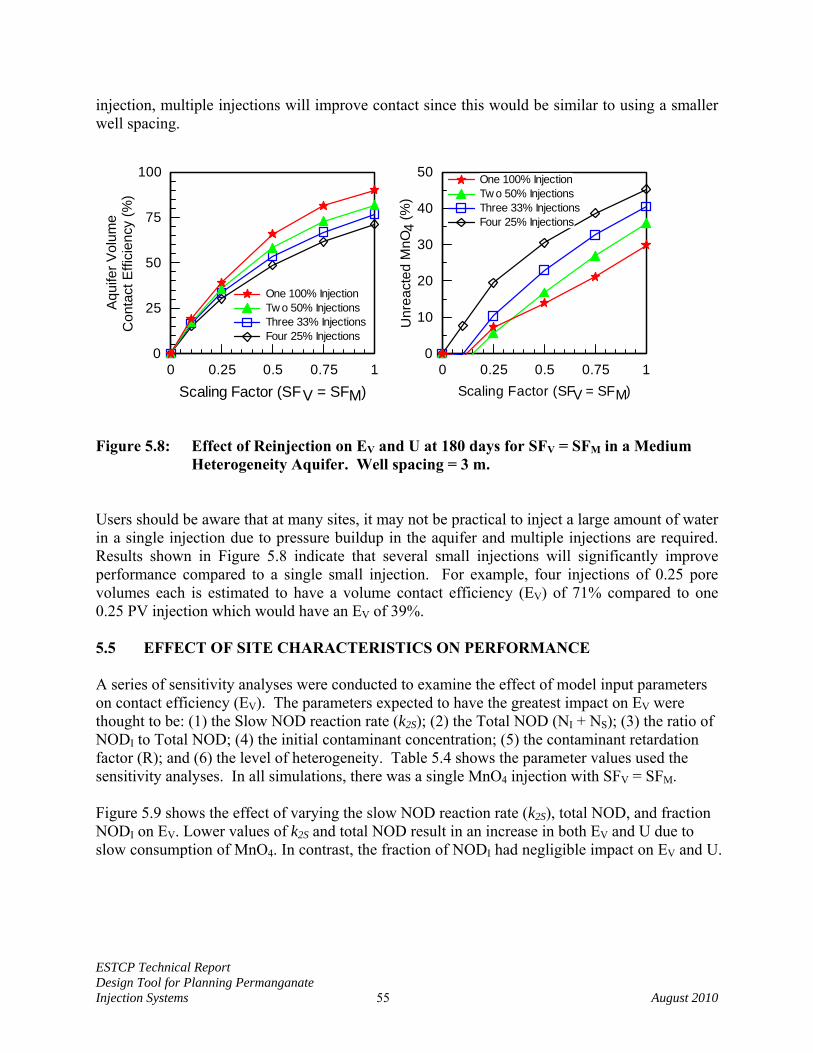
ESTCP Technical Report Design Tool for Planning Permanganate Injection Systems 55 August 2010
injection, multiple injections will improve contact since this would be similar to using a smaller well spacing.
0 0.25 0.5 0.75 1Scaling Factor (SFV = SFM)
0
10
20
30
40
50
Unr
eact
ed M
nO4
(%)
One 100% InjectionTw o 50% InjectionsThree 33% InjectionsFour 25% Injections
0 0.25 0.5 0.75 1Scaling Factor (SFV = SFM)
0
25
50
75
100
Aqui
fer V
olum
eC
onta
ct E
ffici
ency
(%)
One 100% InjectionTw o 50% InjectionsThree 33% InjectionsFour 25% Injections
Figure 5.8: Effect of Reinjection on EV and U at 180 days for SFV = SFM in a Medium Heterogeneity Aquifer. Well spacing = 3 m.
Users should be aware that at many sites, it may not be practical to inject a large amount of water in a single injection due to pressure buildup in the aquifer and multiple injections are required. Results shown in Figure 5.8 indicate that several small injections will significantly improve performance compared to a single small injection. For example, four injections of 0.25 pore volumes each is estimated to have a volume contact efficiency (EV) of 71% compared to one 0.25 PV injection which would have an EV of 39%. 5.5 EFFECT OF SITE CHARACTERISTICS ON PERFORMANCE A series of sensitivity analyses were conducted to examine the effect of model input parameters on contact efficiency (EV). The parameters expected to have the greatest impact on EV were thought to be: (1) the Slow NOD reaction rate (k2S); (2) the Total NOD (NI + NS); (3) the ratio of NODI to Total NOD; (4) the initial contaminant concentration; (5) the contaminant retardation factor (R); and (6) the level of heterogeneity. Table 5.4 shows the parameter values used the sensitivity analyses. In all simulations, there was a single MnO4 injection with SFV = SFM. Figure 5.9 shows the effect of varying the slow NOD reaction rate (k2S), total NOD, and fraction NODI on EV. Lower values of k2S and total NOD result in an increase in both EV and U due to slow consumption of MnO4. In contrast, the fraction of NODI had negligible impact on EV and U.
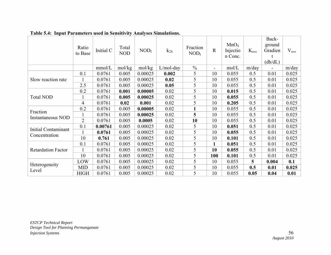
ESTCP Technical Report Design Tool for Planning Permanganate Injection Systems 56 August 2010
Table 5.4: Input Parameters used in Sensitivity Analyses Simulations.
Ratio to Base Initial C Total
NOD NODI k2S Fraction NODI
R MnO4
Injection Conc.
Kave
Back-groundGradien
t (dh/dL)
Vave
mmol/L mol/kg mol/kg L/mol-day % - mol/L m/day - m/day
Slow reaction rate 0.1 0.0761 0.005 0.00025 0.002 5 10 0.055 0.5 0.01 0.025 1 0.0761 0.005 0.00025 0.02 5 10 0.055 0.5 0.01 0.025
2.5 0.0761 0.005 0.00025 0.05 5 10 0.055 0.5 0.01 0.025
Total NOD 0.2 0.0761 0.001 0.00005 0.02 5 10 0.015 0.5 0.01 0.025 1 0.0761 0.005 0.00025 0.02 5 10 0.055 0.5 0.01 0.025 4 0.0761 0.02 0.001 0.02 5 10 0.205 0.5 0.01 0.025
Fraction Instantaneous NOD
0.2 0.0761 0.005 0.00005 0.02 1 10 0.055 0.5 0.01 0.025 1 0.0761 0.005 0.00025 0.02 5 10 0.055 0.5 0.01 0.025 2 0.0761 0.005 0.0005 0.02 10 10 0.055 0.5 0.01 0.025
Initial Contaminant Concentration
0.1 0.00761 0.005 0.00025 0.02 5 10 0.051 0.5 0.01 0.025 1 0.0761 0.005 0.00025 0.02 5 10 0.055 0.5 0.01 0.025 10 0.761 0.005 0.00025 0.02 5 10 0.101 0.5 0.01 0.025
Retardation Factor 0.1 0.0761 0.005 0.00025 0.02 5 1 0.051 0.5 0.01 0.025 1 0.0761 0.005 0.00025 0.02 5 10 0.055 0.5 0.01 0.025 10 0.0761 0.005 0.00025 0.02 5 100 0.101 0.5 0.01 0.025
Heterogeneity Level
LOW 0.0761 0.005 0.00025 0.02 5 10 0.055 5 0.004 0.1 MID 0.0761 0.005 0.00025 0.02 5 10 0.055 0.5 0.01 0.025
HIGH 0.0761 0.005 0.00025 0.02 5 10 0.055 0.05 0.04 0.01
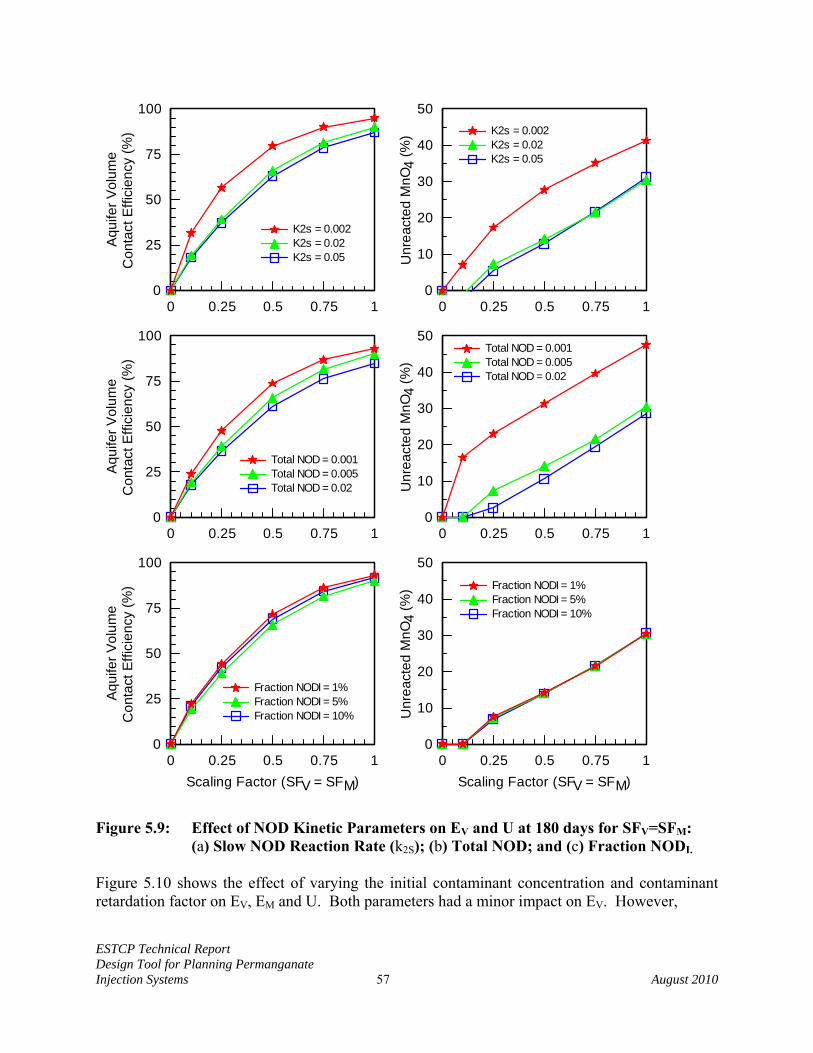
ESTCP Technical Report Design Tool for Planning Permanganate Injection Systems 57 August 2010
0 0.25 0.5 0.75 10
25
50
75
100A
quife
r Vol
ume
Con
tact
Effi
cien
cy (%
)
K2s = 0.002K2s = 0.02K2s = 0.05
0 0.25 0.5 0.75 10
25
50
75
100
Aqui
fer V
olum
e C
onta
ct E
ffici
ency
(%)
Total NOD = 0.001Total NOD = 0.005Total NOD = 0.02
0 0.25 0.5 0.75 1Scaling Factor (SFV = SFM)
0
25
50
75
100
Aqui
fer V
olum
e C
onta
ct E
ffici
ency
(%)
Fraction NODI = 1%Fraction NODI = 5%Fraction NODI = 10%
0 0.25 0.5 0.75 10
10
20
30
40
50
Unr
eact
ed M
nO4
(%) K2s = 0.002
K2s = 0.02K2s = 0.05
0 0.25 0.5 0.75 10
10
20
30
40
50
Unr
eact
ed M
nO4
(%)
Total NOD = 0.001Total NOD = 0.005Total NOD = 0.02
0 0.25 0.5 0.75 1Scaling Factor (SFV = SFM)
0
10
20
30
40
50
Unr
eact
ed M
nO4
(%) Fraction NODI = 1%
Fraction NODI = 5%Fraction NODI = 10%
Figure 5.9: Effect of NOD Kinetic Parameters on EV and U at 180 days for SFV=SFM:
(a) Slow NOD Reaction Rate (k2S); (b) Total NOD; and (c) Fraction NODI. Figure 5.10 shows the effect of varying the initial contaminant concentration and contaminant retardation factor on EV, EM and U. Both parameters had a minor impact on EV. However,
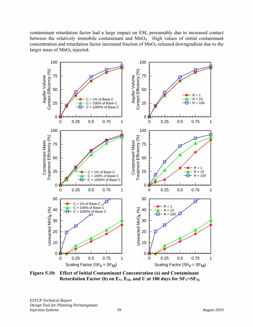
ESTCP Technical Report Design Tool for Planning Permanganate Injection Systems 58 August 2010
contaminant retardation factor had a large impact on EM, presumably due to increased contact between the relatively immobile contaminant and MnO4. High values of initial contaminant concentration and retardation factor increased fraction of MnO4 released downgradient due to the larger mass of MnO4 injected.
0 0.25 0.5 0.75 10
25
50
75
100
Aqu
ifer V
olum
e C
onta
ct E
ffici
ency
(%)
C = 1% of Base CC = 100% of Base CC = 1000% of Base C
0 0.25 0.5 0.75 10
25
50
75
100
Aqu
ifer V
olum
e C
onta
ct E
ffici
ency
(%)
R = 1R = 10R = 100
0 0.25 0.5 0.75 1Scaling Factor (SFV = SFM)
0
10
20
30
40
50
Unr
eact
ed M
nO4
(%)
C = 1% of Base CC = 100% of Base CC = 1000% of Base C
0 0.25 0.5 0.75 1Scaling Factor (SFV = SFM)
0
10
20
30
40
50
Unr
eact
ed M
nO4
(%) R = 1
R = 10R = 100
0 0.25 0.5 0.75 10
25
50
75
100
Con
tam
inan
t Mas
sTr
eatm
ent E
ffici
ency
(%)
C = 1% of Base CC = 100% of Base CC = 1000% of Base C
0 0.25 0.5 0.75 10
25
50
75
100C
onta
min
ant M
ass
Trea
tmen
t Effi
cien
cy (%
)
R = 1R = 10R = 100
Figure 5.10: Effect of Initial Contaminant Concentration (a) and Contaminant
Retardation Factor (b) on EV, EM, and U at 180 days for SFV=SFM.

ESTCP Technical Report Design Tool for Planning Permanganate Injection Systems 59 August 2010
5.5.1 EFFECT OF AQUIFER HETEROGENEITY ON EM Figure 5.11 shows the effect of varying the level of aquifer heterogeneity on EV, EM and U. The error bars represent the standard deviation of these values obtained for the five different realizations simulated for each level of heterogeneity (see Table 5.2 and 5.3). For a given volume of MnO4 solution injected, aquifer volume contact efficiency (EV) is highest and U is lowest for the low heterogeneity permeability distribution. EV decreases and U increases as the level of heterogeneity increases. This is due to flow bypassing around lower permeability zones, causing these zones to remain uncontacted. Aquifer heterogeneity appears to have a complex interaction with contaminant mass removal. EM is highest for the moderate and high heterogeneity simulations. For volume and mass scaling factors (SFV and SFM) less than 0.75, the medium and high heterogeneity distributions result in a somewhat higher treatment efficiency than the low heterogeneity distribution. However, for SFV=SFM=1, EM is lower for the high heterogeneity simulations than the moderate and low heterogeneity simulations. The presence of higher permeability channels in the moderate and high heterogeneity simulations may allow more rapid transport of MnO4 away from the injection well when only a small amount of fluid is injected. Once MnO4 is distributed throughout the treatment zone, contaminants can diffuse out of lower permeability layers and come in contact with MnO4, somewhat increasing EM. However for large values of SFV and SFM, permanganate cannot penetrate the lower permeability zones, reducing the maximum level of treatment that can be achieved.
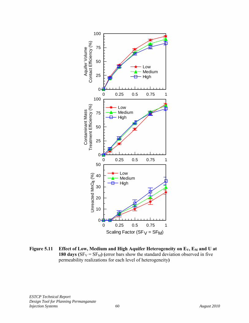
ESTCP Technical Report Design Tool for Planning Permanganate Injection Systems 60 August 2010
0 0.25 0.5 0.75 10
25
50
75
100
Aqu
ifer V
olum
eC
onta
ct E
ffici
ency
(%)
LowMediumHigh
0 0.25 0.5 0.75 10
25
50
75
100
Con
tam
inan
t Mas
s Tr
eatm
ent E
ffici
ency
(%)
LowMediumHigh
0 0.25 0.5 0.75 1Scaling Factor (SFV = SFM)
0
10
20
30
40
50
Unr
eact
ed M
nO4
(%) Low
MediumHigh
Figure 5.11 Effect of Low, Medium and High Aquifer Heterogeneity on EV, EM and U at 180 days (SFV = SFM) (error bars show the standard deviation observed in five permeability realizations for each level of heterogeneity)
ESTCP Technical Report Design Tool for Planning Permanganate Injection Systems 61 August 2010
5.6 SUMMARY AND CONCLUSIONS – EFFECT OF INJECTION SYSTEM DESIGN VARIABLES AND SITE CHARACTERISTICS ON REMEDIATION SYSTEM PERFORMANCE
The ISCO numerical model developed in Section 3 was applied to a hypothetical heterogeneous aquifer to evaluate the effect of different design variables and aquifer parameters on treatment efficiency. Model simulation results indicate that the two parameters with the greatest impact on aquifer contact efficiency and pollutant treatment efficiency are: (1) the mass of permanganate injected; and (2) the volume of water injected. To allow easy comparison between different simulations, the mass of permanganate injected and volume of fluid injected were represented as dimensionless scaling factors. The volume scaling factor (SFV) is the ratio of fluid volume injected to the pore volume of the target treatment zone. The mass scaling factor (SFM) is the ratio of reagent injected to the ultimate oxidant demand (UOD) of the target treatment zone. When small amounts of permanganate are injected, the reagent is rapidly consumed and pollutant removal efficiency does not increase with time after the first 30 days. However, when larger amounts of permanganate are injected, the reagent can persist for several months resulting in a gradual increase in treatment efficiency with time. For constant permanganate mass, increasing fluid volume injected initially results in an improvement in treatment efficiency. However, further increases in fluid volume injected result in little additional benefit. Conversely, when fluid volume is held constant and permanganate mass is increased, treatment efficiency steadily increases, due to down-gradient drift/dispersion of permanganate when larger amounts of reagent are injected. However, increasing mass of MnO4 injected, also incrases the amount of MnO4 that migrates out of the target treatment zone (indicated by increasing fraction unreacted MnO4). Common approaches for improving remediation system performance include: (a) reducing the injection well spacing; and (b) performing multiple MnO4 injections in the same well. Numerical model simulation results indicate that well spacing within a row, and row spacing have a modest impact on volume contact efficiency (EV) and fraction unreacted MnO4 (U) for small amounts of MnO4 and fluid injected (SFV and SFM < 0.25). However for larger amounts of reagent and fluid injected, increasing row spacing had a substantial negative impact, reducing volume contact efficiency and increasing the amount of unreacted MnO4 released downgradient. Numerical model simulation results indicate that, if the total volume of fluid injected and mass of reagent is held constant, multiple injection events will not increase contact efficiency compared to a single large injection event, and can increase the amount of unreacted MnO4 released downgradient. This occurs because several small injections through the same wells repeatedly treats the same area around the wells, with little increase in the fraction of aquifer contacted. This occurs because several small injections result in more complete removal of NODS near the injection well, compared to a single large injection where the MnO4 is rapidly transported away from the injection well. However at many sites, it may not be practical to inject a large amount of water in a single injection due to pressure buildup in the aquifer and multiple injections are required. In these cases, multiple small injections can significantly improve performance compared to a single small injection. A series of sensitivity analyses were conducted to examine the effect of site characteristics on remediation system performance. The initial contaminant concentration and contaminant

ESTCP Technical Report Design Tool for Planning Permanganate Injection Systems 62 August 2010
retardation factor had only a minor impact on remediation system performance, but did have a large impact on the fraction of MnO4 released downgradient. Lower values of k2S and total NOD result in an increase in both EV and U due to slow consumption of MnO4. In contrast, the fraction of NODI had negligible impact on EV and U. Aquifer heterogeneity has a complex relationship with remediation system performance. Increasing levels of heterogeneity have a negative effect on aquifer volume contact efficiency (EV) and fraction of MnO4 released downgradient (U). However, moderate and high levels of heterogeneity appear to increase contaminant mass treatment efficiency (EM) when only small amounts of MnO4 solution are injected. However, when large amounts of MnO4 solution are injected, EM is lower for high heterogeneity simulations. The presence of higher permeability channels in the moderate and high heterogeneity simulations may allow more rapid transport of MnO4 away from the injection well when only a small amount of fluid is injected, improving contaminant treatment. However, permanganate cannot penetrate the lower permeability zones in highly heterogeneous formations, reducing the maximum level of treatment that can be achieved.
ESTCP Technical Report Design Tool for Planning Permanganate Injection Systems 63 August 2010
6.0 SPREADSHEET BASED MODELING OF PERMANGANATE DISTRIBUTION
6.1 INTRODUCTION Permanganate injection can be very effective for ISCO of a variety of ground water contaminants. However to be effective, the permanganate must be brought into close contact with the target contaminant. Simulation results presented in Section 4 indicate that aquifer volume contact efficiency will be controlled by a variety of factors including the mass of permanganate injected, water volume injected, aquifer heterogeneity and kinetics of permanganate consumption by NOD. Detailed injection system designs can be evaluated using the ISCO module developed and tested in Section 3. However, use of this advanced model is not practical in many cases due to time, budget and data constraints. Simple, easy to use tools are needed to assist designers in developing lower cost, more effective remediation systems. In this section, we describe the development and implementation of an Excel-based spreadsheet tool to plan CDISCO. Permanganate transport and consumption in a homogeneous aquifer are simulated using the kinetic approach developed and applied in Sections 3 and4. The effective ROI is then determined based on a user specified contact time and critical permanganate concentration. The ROI is then used to determine required well spacing, injection parameters and generate preliminary cost estimates. Injection parameters can be quickly changed allowing designers to easily evaluate multiple alternatives, allowing designers to quickly identify lower cost, more effective designs. This model is implemented as part of the CDISCO design tool developed with support from the Environmental Technology Certification Program (ESTCP) under project ER-0623 and ER-0625. 6.2 SIMULATING OXIDANT DISTRIBUTION USING A SERIES OF CSTRS 6.2.1 MODEL DEVELOPMENT The transport and consumption of permanganate are simulated within the CDISCO model using the same differential equations developed and tested in Section 3. Based on user input data, the model establishes a series of continuously stirred tank reactors (CSTR) to simulate advective-dispersive transport of permanganate away from a central injection well. Formally, this is a special case of the fully upwinded finite difference solution corrected for numerical dispersion presented by Van Genuchten and Wierenga (1974). Numerical dispersion associated with evaluation of the time derivative is negligible (Van Genuchten and Wierenga, 1974) so longitudinal dispersion is simulated by setting the length of each reactor to two times the longitudinal dispersivity (αL). The volume of each CSTR reactor increases outward from the injection well, simulating the decline in velocity during radial flow. The volume of the first reactor (V1) is Be n π (αL)2 where Be is the effective saturate thickness and n is porosity. The volume of each additional reactor VN is Be n π [(αL +2(N-1) αL))2 - (αL +2(N-2) αL))2] where N is the reactor number.
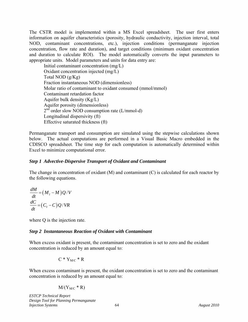
ESTCP Technical Report Design Tool for Planning Permanganate Injection Systems 64 August 2010
The CSTR model is implemented within a MS Excel spreadsheet. The user first enters information on aquifer characteristics (porosity, hydraulic conductivity, injection interval, total NOD, contaminant concentrations, etc.), injection conditions (permanganate injection concentration, flow rate and duration), and target conditions (minimum oxidant concentration and duration to calculate ROI). The model automatically converts the input parameters to appropriate units. Model parameters and units for data entry are:
Initial contaminant concentration (mg/L) Oxidant concentration injected (mg/L) Total NOD (g/Kg) Fraction instantaneous NOD (dimensionless) Molar ratio of contaminant to oxidant consumed (mmol/mmol) Contaminant retardation factor Aquifer bulk density (Kg/L) Aquifer porosity (dimensionless) 2nd order slow NOD consumption rate (L/mmol-d) Longitudinal dispersivity (ft) Effective saturated thickness (ft)
Permanganate transport and consumption are simulated using the stepwise calculations shown below. The actual computations are performed in a Visual Basic Macro embedded in the CDISCO spreadsheet. The time step for each computation is automatically determined within Excel to minimize computational error. Step 1 Advective-Dispersive Transport of Oxidant and Contaminant The change in concentration of oxidant (M) and contaminant (C) is calculated for each reactor by the following equations.
( ) /IdM M M Q Vdt
= −
( ) /IdC C C Q VRdt
= −
where Q is the injection rate. Step 2 Instantaneous Reaction of Oxidant with Contaminant When excess oxidant is present, the contaminant concentration is set to zero and the oxidant concentration is reduced by an amount equal to: C * YM/C * R When excess contaminant is present, the oxidant concentration is set to zero and the contaminant concentration is reduced by an amount equal to: M/(YM/C * R)
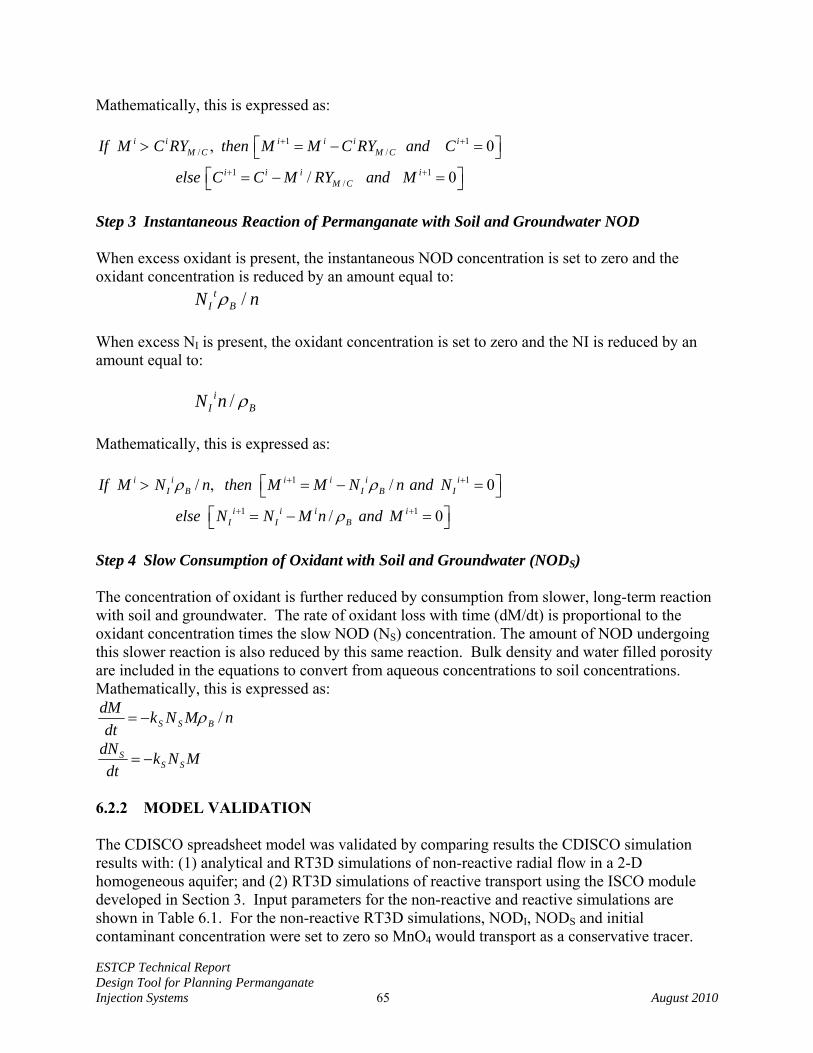
ESTCP Technical Report Design Tool for Planning Permanganate Injection Systems 65 August 2010
Mathematically, this is expressed as:
1 1/ /
1 1/
, 0
/ 0
i i i i i iM C M C
i i i iM C
If M C RY then M M C RY and C
else C C M RY and M
+ +
+ +
⎡ ⎤> = − =⎣ ⎦⎡ ⎤= − =⎣ ⎦
Step 3 Instantaneous Reaction of Permanganate with Soil and Groundwater NOD When excess oxidant is present, the instantaneous NOD concentration is set to zero and the oxidant concentration is reduced by an amount equal to:
/tI BN nρ
When excess NI is present, the oxidant concentration is set to zero and the NI is reduced by an amount equal to:
/iI BN n ρ
Mathematically, this is expressed as:
1 1
1 1
/ , / 0
/ 0
i i i i i iI B I B I
i i i iI I B
If M N n then M M N n and N
else N N M n and M
ρ ρ
ρ
+ +
+ +
⎡ ⎤> = − =⎣ ⎦⎡ ⎤= − =⎣ ⎦
Step 4 Slow Consumption of Oxidant with Soil and Groundwater (NODS) The concentration of oxidant is further reduced by consumption from slower, long-term reaction with soil and groundwater. The rate of oxidant loss with time (dM/dt) is proportional to the oxidant concentration times the slow NOD (NS) concentration. The amount of NOD undergoing this slower reaction is also reduced by this same reaction. Bulk density and water filled porosity are included in the equations to convert from aqueous concentrations to soil concentrations. Mathematically, this is expressed as:
nMNkdt
dMBSS /ρ−=
MNk
dtdN
SSS −=
6.2.2 MODEL VALIDATION The CDISCO spreadsheet model was validated by comparing results the CDISCO simulation results with: (1) analytical and RT3D simulations of non-reactive radial flow in a 2-D homogeneous aquifer; and (2) RT3D simulations of reactive transport using the ISCO module developed in Section 3. Input parameters for the non-reactive and reactive simulations are shown in Table 6.1. For the non-reactive RT3D simulations, NODI, NODS and initial contaminant concentration were set to zero so MnO4 would transport as a conservative tracer.
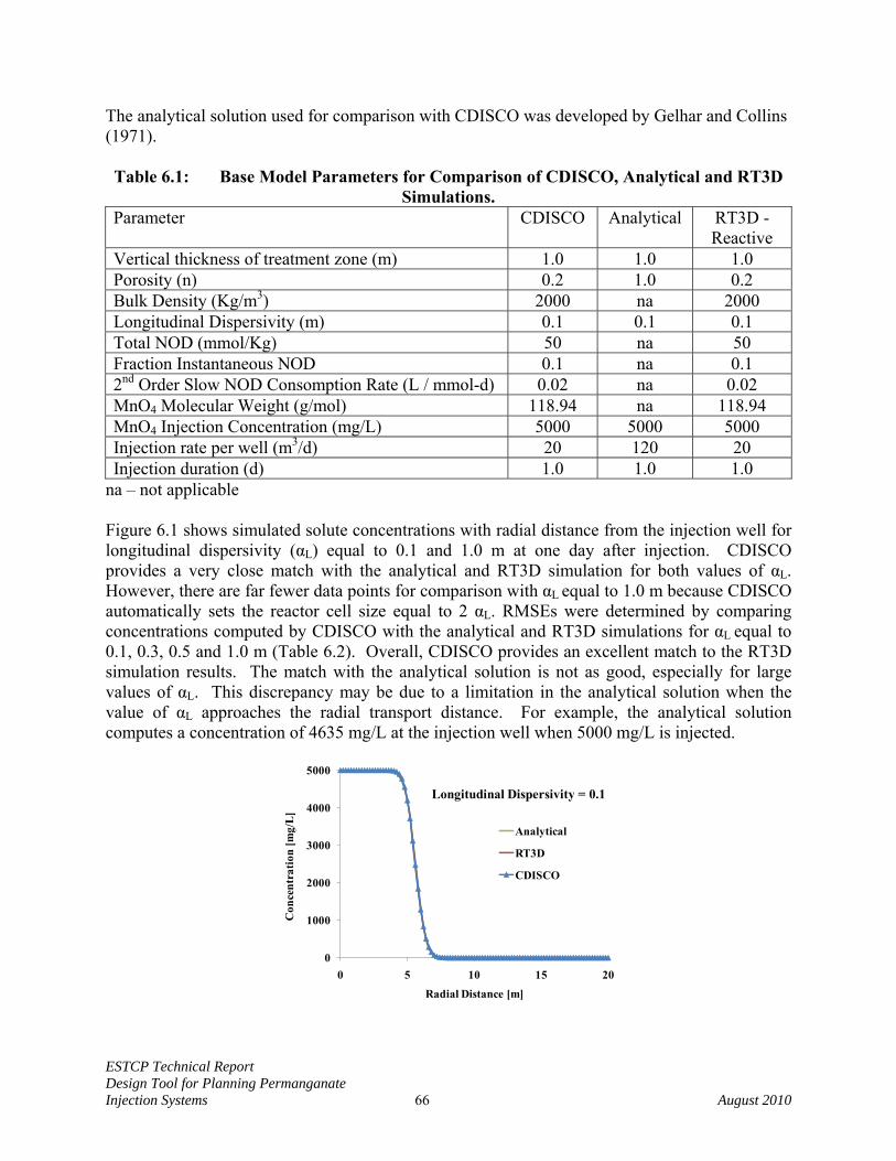
ESTCP Technical Report Design Tool for Planning Permanganate Injection Systems 66 August 2010
The analytical solution used for comparison with CDISCO was developed by Gelhar and Collins (1971). Table 6.1: Base Model Parameters for Comparison of CDISCO, Analytical and RT3D
Simulations. Parameter CDISCO Analytical RT3D -
Reactive Vertical thickness of treatment zone (m) 1.0 1.0 1.0 Porosity (n) 0.2 1.0 0.2 Bulk Density (Kg/m3) 2000 na 2000 Longitudinal Dispersivity (m) 0.1 0.1 0.1 Total NOD (mmol/Kg) 50 na 50 Fraction Instantaneous NOD 0.1 na 0.1 2nd Order Slow NOD Consomption Rate (L / mmol-d) 0.02 na 0.02 MnO4 Molecular Weight (g/mol) 118.94 na 118.94 MnO4 Injection Concentration (mg/L) 5000 5000 5000 Injection rate per well (m3/d) 20 120 20 Injection duration (d) 1.0 1.0 1.0
na – not applicable Figure 6.1 shows simulated solute concentrations with radial distance from the injection well for longitudinal dispersivity (αL) equal to 0.1 and 1.0 m at one day after injection. CDISCO provides a very close match with the analytical and RT3D simulation for both values of αL. However, there are far fewer data points for comparison with αL equal to 1.0 m because CDISCO automatically sets the reactor cell size equal to 2 αL. RMSEs were determined by comparing concentrations computed by CDISCO with the analytical and RT3D simulations for αL equal to 0.1, 0.3, 0.5 and 1.0 m (Table 6.2). Overall, CDISCO provides an excellent match to the RT3D simulation results. The match with the analytical solution is not as good, especially for large values of αL. This discrepancy may be due to a limitation in the analytical solution when the value of αL approaches the radial transport distance. For example, the analytical solution computes a concentration of 4635 mg/L at the injection well when 5000 mg/L is injected.
0
1000
2000
3000
4000
5000
0 5 10 15 20
Con
cent
ratio
n [m
g/L
]
Radial Distance [m]
Longitudinal Dispersivity = 0.1
Analytical
RT3D
CDISCO
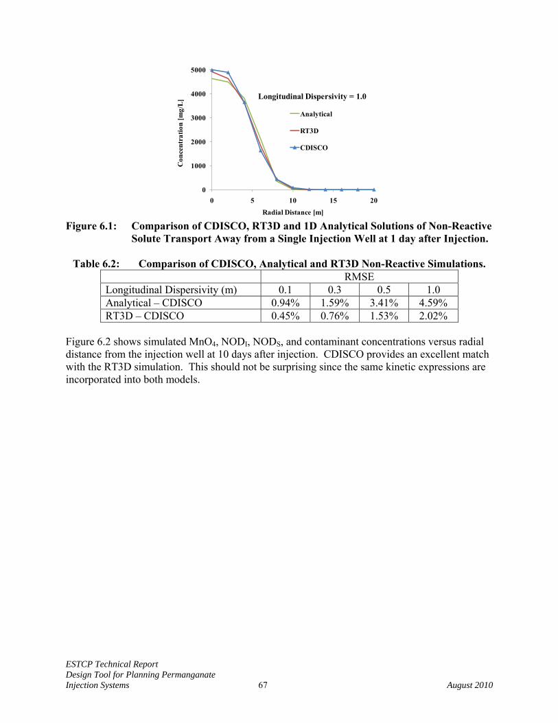
ESTCP Technical Report Design Tool for Planning Permanganate Injection Systems 67 August 2010
0
1000
2000
3000
4000
5000
0 5 10 15 20
Con
cent
ratio
n [m
g/L
]
Radial Distance [m]
Longitudinal Dispersivity = 1.0
Analytical
RT3D
CDISCO
Figure 6.1: Comparison of CDISCO, RT3D and 1D Analytical Solutions of Non-Reactive
Solute Transport Away from a Single Injection Well at 1 day after Injection.
Table 6.2: Comparison of CDISCO, Analytical and RT3D Non-Reactive Simulations. RMSE Longitudinal Dispersivity (m) 0.1 0.3 0.5 1.0 Analytical – CDISCO 0.94% 1.59% 3.41% 4.59% RT3D – CDISCO 0.45% 0.76% 1.53% 2.02%
Figure 6.2 shows simulated MnO4, NODI, NODS, and contaminant concentrations versus radial distance from the injection well at 10 days after injection. CDISCO provides an excellent match with the RT3D simulation. This should not be surprising since the same kinetic expressions are incorporated into both models.
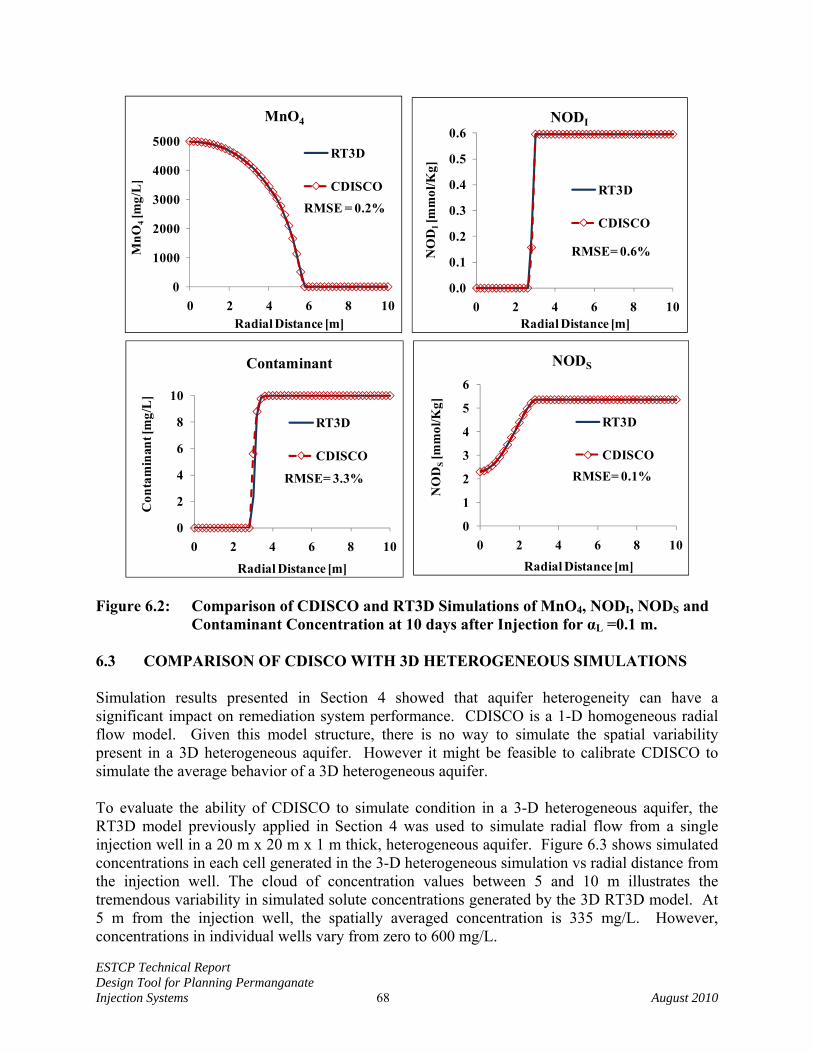
ESTCP Technical Report Design Tool for Planning Permanganate Injection Systems 68 August 2010
0
1000
2000
3000
4000
5000
0 2 4 6 8 10
MnO
4[m
g/L
]
Radial Distance [m]
MnO4
RT3D
CDISCO
0
2
4
6
8
10
0 2 4 6 8 10
Con
tam
inan
t [m
g/L
]
Radial Distance [m]
Contaminant
RT3D
CDISCO
RMSE= 3.3%
0.0
0.1
0.2
0.3
0.4
0.5
0.6
0 2 4 6 8 10
NO
DI[m
mol
/Kg]
Radial Distance [m]
NODI
RT3D
CDISCO
0
1
2
3
4
5
6
0 2 4 6 8 10
NO
DS
[mm
ol/K
g]
Radial Distance [m]
NODS
RT3D
CDISCORMSE= 0.1%
RMSE = 0.2%
RMSE= 0.6%
Figure 6.2: Comparison of CDISCO and RT3D Simulations of MnO4, NODI, NODS and
Contaminant Concentration at 10 days after Injection for αL =0.1 m. 6.3 COMPARISON OF CDISCO WITH 3D HETEROGENEOUS SIMULATIONS Simulation results presented in Section 4 showed that aquifer heterogeneity can have a significant impact on remediation system performance. CDISCO is a 1-D homogeneous radial flow model. Given this model structure, there is no way to simulate the spatial variability present in a 3D heterogeneous aquifer. However it might be feasible to calibrate CDISCO to simulate the average behavior of a 3D heterogeneous aquifer. To evaluate the ability of CDISCO to simulate condition in a 3-D heterogeneous aquifer, the RT3D model previously applied in Section 4 was used to simulate radial flow from a single injection well in a 20 m x 20 m x 1 m thick, heterogeneous aquifer. Figure 6.3 shows simulated concentrations in each cell generated in the 3-D heterogeneous simulation vs radial distance from the injection well. The cloud of concentration values between 5 and 10 m illustrates the tremendous variability in simulated solute concentrations generated by the 3D RT3D model. At 5 m from the injection well, the spatially averaged concentration is 335 mg/L. However, concentrations in individual wells vary from zero to 600 mg/L.
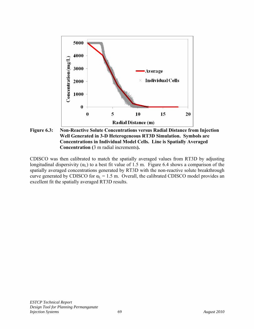
ESTCP Technical Report Design Tool for Planning Permanganate Injection Systems 69 August 2010
Figure 6.3: Non-Reactive Solute Concentrations versus Radial Distance from Injection
Well Generated in 3-D Heterogeneous RT3D Simulation. Symbols are Concentrations in Individual Model Cells. Line is Spatially Averaged Concentration (3 m radial increments).
CDISCO was then calibrated to match the spatially averaged values from RT3D by adjusting longitudinal dispersivity (αL) to a best fit value of 1.5 m. Figure 6.4 shows a comparison of the spatially averaged concentrations generated by RT3D with the non-reactive solute breakthrough curve generated by CDISCO for αL = 1.5 m. Overall, the calibrated CDISCO model provides an excellent fit the spatially averaged RT3D results.
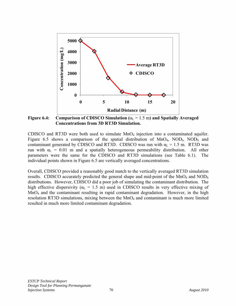
ESTCP Technical Report Design Tool for Planning Permanganate Injection Systems 70 August 2010
0
1000
2000
3000
4000
5000
0 5 10 15 20
Con
cent
ratio
n (m
g/L
)
Radial Distance (m)
Average RT3D
CDISCO
Figure 6.4: Comparison of CDISCO Simulation (αL = 1.5 m) and Spatially Averaged
Concentrations from 3D RT3D Simulation. CDISCO and RT3D were both used to simulate MnO4 injection into a contaminated aquifer. Figure 6.5 shows a comparison of the spatial distribution of MnO4, NODI, NODS and contaminant generated by CDISCO and RT3D. CDISCO was run with αL = 1.5 m. RT3D was run with αL = 0.01 m and a spatially heterogeneous permeability distribution. All other parameters were the same for the CDISCO and RT3D simulations (see Table 6.1). The individual points shown in Figure 6.5 are vertically averaged concentrations. Overall, CDISCO provided a reasonably good match to the vertically averaged RT3D simulation results. CDISCO accurately predicted the general shape and mid-point of the MnO4 and NODS distributions. However, CDISCO did a poor job of simulating the contaminant distribution. The high effective dispersivity (αL = 1.5 m) used in CDISCO results in very effective mixing of MnO4 and the contaminant resulting in rapid contaminant degradation. However, in the high resolution RT3D simulations, mixing between the MnO4 and contaminant is much more limited resulted in much more limited contaminant degradation.
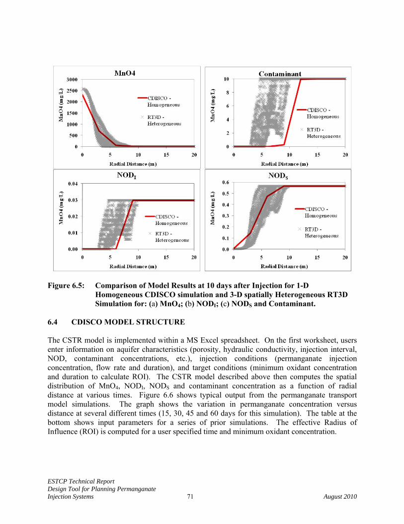
ESTCP Technical Report Design Tool for Planning Permanganate Injection Systems 71 August 2010
Figure 6.5: Comparison of Model Results at 10 days after Injection for 1-D Homogeneous CDISCO simulation and 3-D spatially Heterogeneous RT3D Simulation for: (a) MnO4; (b) NODI; (c) NODS and Contaminant.
6.4 CDISCO MODEL STRUCTURE The CSTR model is implemented within a MS Excel spreadsheet. On the first worksheet, users enter information on aquifer characteristics (porosity, hydraulic conductivity, injection interval, NOD, contaminant concentrations, etc.), injection conditions (permanganate injection concentration, flow rate and duration), and target conditions (minimum oxidant concentration and duration to calculate ROI). The CSTR model described above then computes the spatial distribution of MnO4, NODI, NODS and contaminant concentration as a function of radial distance at various times. Figure 6.6 shows typical output from the permanganate transport model simulations. The graph shows the variation in permanganate concentration versus distance at several different times (15, 30, 45 and 60 days for this simulation). The table at the bottom shows input parameters for a series of prior simulations. The effective Radius of Influence (ROI) is computed for a user specified time and minimum oxidant concentration.
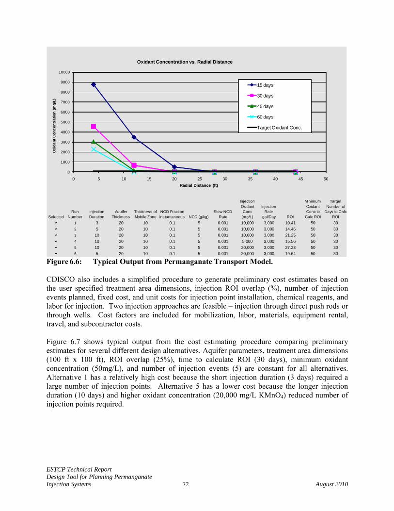
ESTCP Technical Report Design Tool for Planning Permanganate Injection Systems 72 August 2010
SelectedRun
NumberInjection Duration
Aquifer Thickness
Thickness of Mobile Zone
NOD Fraction Instantaneous NOD (g/kg)
Slow NOD Rate
Injection Oxidant Conc
(mg/L)
Injection Rate
gal/Day ROI
Minimum Oxidant Conc to
Calc ROI
Target Number of
Days to CalcROI
a 1 3 20 10 0.1 5 0.001 10,000 3,000 10.41 50 30a 2 5 20 10 0.1 5 0.001 10,000 3,000 14.46 50 30a 3 10 20 10 0.1 5 0.001 10,000 3,000 21.25 50 30a 4 10 20 10 0.1 5 0.001 5,000 3,000 15.56 50 30a 5 10 20 10 0.1 5 0.001 20,000 3,000 27.23 50 30a 6 5 20 10 0.1 5 0.001 20,000 3,000 19.64 50 30
0
1000
2000
3000
4000
5000
6000
7000
8000
9000
10000
0 5 10 15 20 25 30 35 40 45 50
Oxi
dant
Con
cent
ratio
n (m
g/L)
Radial Distance (ft)
Oxidant Concentration vs. Radial Distance
15 days
30 days
45 days
60 days
Target Oxidant Conc.
Figure 6.6: Typical Output from Permanganate Transport Model. CDISCO also includes a simplified procedure to generate preliminary cost estimates based on the user specified treatment area dimensions, injection ROI overlap (%), number of injection events planned, fixed cost, and unit costs for injection point installation, chemical reagents, and labor for injection. Two injection approaches are feasible – injection through direct push rods or through wells. Cost factors are included for mobilization, labor, materials, equipment rental, travel, and subcontractor costs. Figure 6.7 shows typical output from the cost estimating procedure comparing preliminary estimates for several different design alternatives. Aquifer parameters, treatment area dimensions (100 ft x 100 ft), ROI overlap (25%), time to calculate ROI (30 days), minimum oxidant concentration (50mg/L), and number of injection events (5) are constant for all alternatives. Alternative 1 has a relatively high cost because the short injection duration (3 days) required a large number of injection points. Alternative 5 has a lower cost because the longer injection duration (10 days) and higher oxidant concentration (20,000 mg/L KMnO4) reduced number of injection points required.
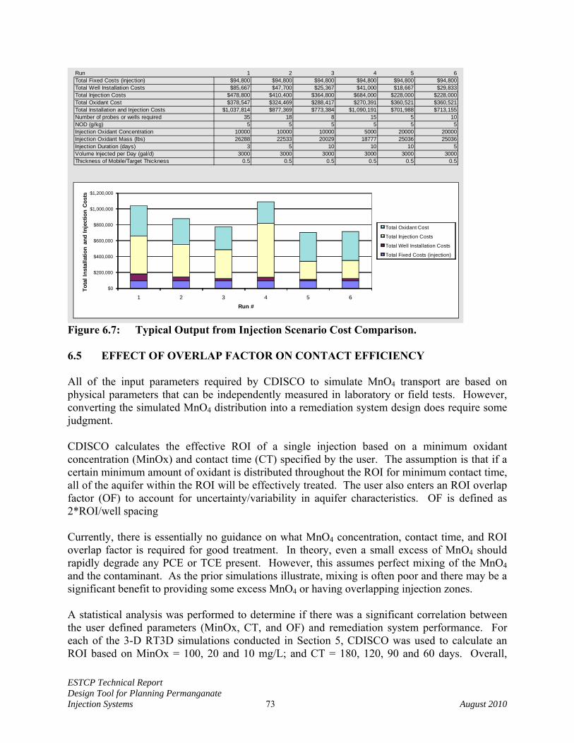
ESTCP Technical Report Design Tool for Planning Permanganate Injection Systems 73 August 2010
Run 1 2 3 4 5 6Total Fixed Costs (injection) $94,800 $94,800 $94,800 $94,800 $94,800 $94,800Total Well Installation Costs $85,667 $47,700 $25,367 $41,000 $18,667 $29,833Total Injection Costs $478,800 $410,400 $364,800 $684,000 $228,000 $228,000Total Oxidant Cost $378,547 $324,469 $288,417 $270,391 $360,521 $360,521Total Installation and Injection Costs $1,037,814 $877,369 $773,384 $1,090,191 $701,988 $713,155Number of probes or wells required 35 18 8 15 5 10NOD (g/kg) 5 5 5 5 5 5Injection Oxidant Concentration 10000 10000 10000 5000 20000 20000Injection Oxidant Mass (lbs) 26288 22533 20029 18777 25036 25036Injection Duration (days) 3 5 10 10 10 5Volume Injected per Day (gal/d) 3000 3000 3000 3000 3000 3000Thickness of Mobile/Target Thickness 0.5 0.5 0.5 0.5 0.5 0.5
00
$0
$200,000
$400,000
$600,000
$800,000
$1,000,000
$1,200,000
1 2 3 4 5 6
Tota
l Ins
talla
tion
and
Inje
ctio
n Co
sts
Run #
Total Oxidant Cost
Total Injection Costs
Total Well Installation Costs
Total Fixed Costs (injection)
Figure 6.7: Typical Output from Injection Scenario Cost Comparison. 6.5 EFFECT OF OVERLAP FACTOR ON CONTACT EFFICIENCY All of the input parameters required by CDISCO to simulate MnO4 transport are based on physical parameters that can be independently measured in laboratory or field tests. However, converting the simulated MnO4 distribution into a remediation system design does require some judgment. CDISCO calculates the effective ROI of a single injection based on a minimum oxidant concentration (MinOx) and contact time (CT) specified by the user. The assumption is that if a certain minimum amount of oxidant is distributed throughout the ROI for minimum contact time, all of the aquifer within the ROI will be effectively treated. The user also enters an ROI overlap factor (OF) to account for uncertainty/variability in aquifer characteristics. OF is defined as 2*ROI/well spacing Currently, there is essentially no guidance on what MnO4 concentration, contact time, and ROI overlap factor is required for good treatment. In theory, even a small excess of MnO4 should rapidly degrade any PCE or TCE present. However, this assumes perfect mixing of the MnO4 and the contaminant. As the prior simulations illustrate, mixing is often poor and there may be a significant benefit to providing some excess MnO4 or having overlapping injection zones. A statistical analysis was performed to determine if there was a significant correlation between the user defined parameters (MinOx, CT, and OF) and remediation system performance. For each of the 3-D RT3D simulations conducted in Section 5, CDISCO was used to calculate an ROI based on MinOx = 100, 20 and 10 mg/L; and CT = 180, 120, 90 and 60 days. Overall,
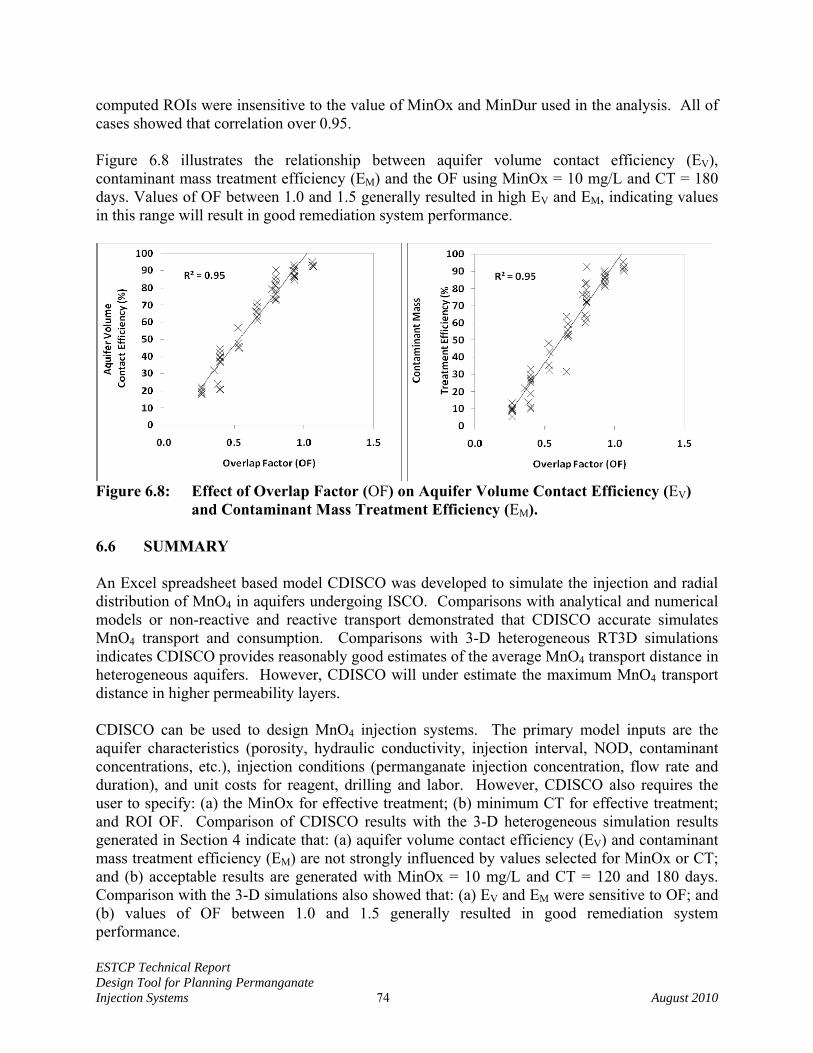
ESTCP Technical Report Design Tool for Planning Permanganate Injection Systems 74 August 2010
computed ROIs were insensitive to the value of MinOx and MinDur used in the analysis. All of cases showed that correlation over 0.95. Figure 6.8 illustrates the relationship between aquifer volume contact efficiency (EV), contaminant mass treatment efficiency (EM) and the OF using MinOx = 10 mg/L and CT = 180 days. Values of OF between 1.0 and 1.5 generally resulted in high EV and EM, indicating values in this range will result in good remediation system performance.
Figure 6.8: Effect of Overlap Factor (OF) on Aquifer Volume Contact Efficiency (EV)
and Contaminant Mass Treatment Efficiency (EM). 6.6 SUMMARY An Excel spreadsheet based model CDISCO was developed to simulate the injection and radial distribution of MnO4 in aquifers undergoing ISCO. Comparisons with analytical and numerical models or non-reactive and reactive transport demonstrated that CDISCO accurate simulates MnO4 transport and consumption. Comparisons with 3-D heterogeneous RT3D simulations indicates CDISCO provides reasonably good estimates of the average MnO4 transport distance in heterogeneous aquifers. However, CDISCO will under estimate the maximum MnO4 transport distance in higher permeability layers. CDISCO can be used to design MnO4 injection systems. The primary model inputs are the aquifer characteristics (porosity, hydraulic conductivity, injection interval, NOD, contaminant concentrations, etc.), injection conditions (permanganate injection concentration, flow rate and duration), and unit costs for reagent, drilling and labor. However, CDISCO also requires the user to specify: (a) the MinOx for effective treatment; (b) minimum CT for effective treatment; and ROI OF. Comparison of CDISCO results with the 3-D heterogeneous simulation results generated in Section 4 indicate that: (a) aquifer volume contact efficiency (EV) and contaminant mass treatment efficiency (EM) are not strongly influenced by values selected for MinOx or CT; and (b) acceptable results are generated with MinOx = 10 mg/L and CT = 120 and 180 days. Comparison with the 3-D simulations also showed that: (a) EV and EM were sensitive to OF; and (b) values of OF between 1.0 and 1.5 generally resulted in good remediation system performance.
ESTCP Technical Report Design Tool for Planning Permanganate Injection Systems 75 August 2010
7.0 REFERENCES AFCEE, (2007a) The Installation Restoration Program at the Massachusetts Military Reservation (MMR), Air Force Center for Engineering and the Environment (http://mmr.org/). AFCEE, (2007b) Groundwater Plume Maps and Information Booklet, Air Force Center for Engineering and the Environment. ATSDR, (2004) Medical Management Guidelines for Tetrachloroethylene, Agency for Toxic Substances and Disease Registry, Division of Toxicology and Environmental Medicine, U.S. ATSDR, (2007) CERCLA Priority List of Hazardous Substances that will be The Subject of Toxicological Profiles and Support Document, Agency for Toxic Substances and Disease Registry, Division of Toxicology and Environmental Medicine, U.S. ASTM D7262, (2007) Standard Test Method for Estimating the Permanganate Natural Oxidant Demand of Soil and Aquifer Solids, In; ASTM International: West Conshohocken, Pennsylvania . CH2M Hill, (2007) Project Note for CS-10 ISCO Pilot Test Work Plan. Chambers, J.D., A.L. Leavitt, C.L. Walti, C.G. Schreier, J.T. Melby, and L. Goldstein, (2000) Treatability Study – Fate of Chromium during Oxidation of Chlorinated Solvents, In: Proceedings of International Conference on Remediation of Chlorinated and Recalcitrant Compounds, Columbus, Ohio, pp. 57-66. Clement, T.P., (1997) RT3D: A Modular Computer Code for Simulation of Reactive Multispecies Transport in 3-Dimensional Groundwater Systems, U.S. Department of Energy. Drescher, E.A., R. Gavaskar, B.M. Sass, L.J. Cumming, M.J. Drescher, and T. Williamson, (1999) Batch and Column Testing to Evaluate Chemical Oxidation of DNAPL Source Areas, In: Proceeding of International Conference on Remediation of Chlorinated and Recalcitrant Compounds, Columbus, Ohio, pp. 425-432. Eilbeck, W.J., and G. Mattock, (1987) Chemical Processes in Wastewater Treatment, John Wiley and Sons, Toronto, Ontario. Gates, D.D., R.L. Siegrist, and S.R. Cline, (1995) Chemical Oxidation of Volatile and semi-Volatile Organic Compounds in Soil, U.S., pg. 17. Gates, D.D., Siegrist, R.L., and Cline, S.R., (2001) Comparison of Potassium Permanganate and Hydrogen Peroxide as Chemical Oxidants for Organically Contaminated Soils, Journal of Environmental Engineering 127(4), pp. 337-347. Gelhar, L.W. and M.A. Collins, (1971) General Analysis of Longitudinal Dispersion in Nonuniform Flow, Water Resources Research. 7(6): 1511-1521.
ESTCP Technical Report Design Tool for Planning Permanganate Injection Systems 76 August 2010
Harbaugh, A.W., E.R. Banta, M.C. Hill, and M.G. McDonald, (2000) MODFLOW-2000, the U.S. Geological Survey Modular Ground-Water Model - User Guide to Modularization Concepts and the Ground-Water Flow Process, Open-File Report 00-92, U.S. Geological Survey, pg. 121. Haselow, J.S., R.L. Siegrist, M. Crimi, and T. Jarosch, (2003) Estimating the Total Oxidant Demand for In Situ Chemical Oxidation Design, Remediation Journal 13(4), pp. 5-16. Hood, E.D., (2000a) Permanganate Flushing of DNAPL Source Zones: Experimental and Numerical Investigation, Civil and Environmental Engineering, Waterloo, University of Waterloo, PhD Dissertation. Hood, E.D., and Thomson N.R., (2000b) Numerical Simulation of In Situ Chemical Oxidation, In: Proceedings of International Conference on Remediation of Chlorinated and Recalcitrant Compounds, Columbus, Ohio, pp. 82–90. Huling, S.G. and B. Pivetz. 2006. “In-Situ Chemical Oxidation - Engineering Issue”. U.S. Environmental Protection Agency, National Risk Management Research Laboratory, R.S. Kerr Environmental Research Center, Ada, OK. EPA/600/R-06/072. (http://www.epa.gov/ada/download/issue/600R06072.pdf). Hutson, S.S., (2004) Estimated Use of Water in the United States in 2000, U.S. Geological Survey, Reston, Virginia. ITRC. 2005. Technical and Regulatory Guidance for In Situ Chemical Oxidation of Contaminated Soil and Groundwater 2nd Edition, ISCO-2. Washington, D.C.: Interstate Technology & Regulatory Council. http://www.itrcweb.org/gd_ISCO.asp Jones, L.J., (2007) The Impact of NOD Reaction Kinetic on Treatment Efficiency, Civil and Environmental Engineering, Waterloo, University of Waterloo, MS Thesis. Leung, S.W., R.J. Watts, and G.C. Miller, (1992) Degradation of Perchloroethylene by Fenton’s Reagent: Speciation and Pathway, Journal of Environmental Quality 21, pp. 377-381. Lowe, K.S., Gardner, F.G., Siegrist R.L., and Houk T.C., (1999) Field Pilot Test of In Situ Chemical Oxidation Through Recirculation Using Vertical Wells at the Portsmouth Gaseous Diffusion Plant, EPA 625-R-99-012, pp. 42-49. Marvin, B.K., J. Chambers, A. Leavitt, and C.G. Schreier, (2002) Chemical and Engineering Challenges to In Situ Permanganate Remediation, Battelle Press, Monterey, California, pp. 1127-1134. McDonald, M.G., and A.W. Harbaugh, (1988) A Modular 3-Dimensional Finite-Difference Ground-Water Flow Model, Techniques of Water-Resources Investigations, Book 6, US Geological Survey, pg. 586.
ESTCP Technical Report Design Tool for Planning Permanganate Injection Systems 77 August 2010
Mumford, K.G., N.R. Thomson, and R.M. Allen-King, (2002) Investigating the Kinetic Nature of Natural Oxidant Demand During ISCO, Battelle Press, Monterey, California, pp. 1383-1388. Mumford, K.G., C.S. Lamarche, and N.R. Thomson, (2004) Natural Oxidant Demand of Aquifer Materials Using the Push-Pull Technique, Journal of Environmental Engineering 130(10), pp. 1139-1146. Mumford, K.G., N.R. Thomson, and R.M. Allen-King, (2005) Bench-Scale Investigation of Permanganate Natural Oxidant Demand Kinetics, Environmental Science and Technology 39(8), pp. 2835-2840. Oberle, D.W., and D.L Schroder, (2000) Design Considerations for In-Situ Chemical Oxidation, Chemical Oxidation and Reactive Barriers; Remediation of Chlorinated and Recalcitrant Compounds, pp. 91-99. Reitsma, S., and Q.L. Dai, (2001) Reaction-Enhanced Mass Transfer and Transport from Non-Aqueous Phase Liquid Source Zones, Journal of Contaminant Hydrology 49(1-2), pp. 49-66. Schnarr, M., C. Truax, G. Farquhar, E. Hood, T. Gonullu, and B. Stickney, (1998) Laboratory and Controlled Field Experiments Using Potassium Permanganate to Remediate Trichloroethylene and Perchloroethylene DNAPLs in Porous Media, Journal of Contaminant Hydrology 29(3), pp. 205-224. Siegrist, R.L., K.S Lowe, L.D. Murdoch, W.W. Slack, and T.C. Houk, (1998a) X-231A Demonstration of In Situ Remediation of DNAPL Compounds in Low Permeability Media by Soil Fracturing with Thermally Enhanced Mass Recovery or Reactive Barrier Destruction, Oak Ridge National Laboratory Report, ORNL/TM-13534. Siegrist, R.L., K.S. Lowe, L.C. Murdoch, T.L. Case, D.A. Pickering, and T.C. Houk, (1998b) Horizontal Treatment Barriers of Fracture-Emplaced Iron and Permanganate Particles, EPA 542-R-98–003, pp. 77-83. Siegrist, R.L., M.A. Urynowicz, and O.R. West, (2000) An Overview of In Situ Chemical Oxidation Technology Features and Applications, EPA 625-R-99-012, pp. 61-69. Siegrist, R.L., M.A. Urynowicz, O.R. West, M.L. Crimi, and K.S. Lowe, (2001) Principles and Practices of In Situ Chemical Oxidation Using Permanganate, Battelle Press, Columbus, OH. Siegrist, R.L., M.L. Crimi, B. Petri, T. Simpkin, T. Palaia, F.J. Krembs, J. Munakata-Marr, T. Illangasekare, G. Ng, M. Singletary, N. Ruiz. 2009. In Situ Chemical Oxidation for Groundwater Remediation: Site Specific Engineering & Technology Application. Final project report to the U.S. Environmental Security Technology Certification Program for ESTCP project ER-0623. Steel, E.W., and T.J. McGhee, T.J., (1979) Water Supply and Sewerage, Fifth Edition, McGraw-Hill, New York, New York.
ESTCP Technical Report Design Tool for Planning Permanganate Injection Systems 78 August 2010
Tompson, A.F.B., R. Aboudu, and L.W. Gelhar, (1989) Implementation of the Three Dimensional Turning Bands Random Field Generator, Water Resources Research 25(10), pp. 2227-2243. US EPA, (1998) Field Applications of In Situ Remediation Technologies: Chemical Oxidation, US Environmental Protection Agency, Solid Waste and Emergency Response, EPA 542-R-98-008 . US EPA, (2007) Treatment Technologies for Site Cleanup: Annual Status Report (Twelfth edition), US Environmental Protection Agency, Solid Waste and Emergency Response, EPA 542-R-07-012. Urynowicz, M.A., B. Balu, and U. Udayasankar, (2008) Kinetics of Natural Oxidant Demand by Permanganate in Aquifer Solids. Journal of Contaminant Hydrology 96(1-4), pp. 187-194. Van Genuchten, M. T., and P. J. Wierenga, (1974) Simulation of one dimensional solute transfer in porous media, Bull. 628, New Mexico State University Agricultural Experiment Station, Las Cruces. Vella, P.A., G. Deshinsky, J.E. Boll, J. Munder, and W.M. Joyce, (1990) Treatment of Low Level Phenols with Potassium Permanganate, Research Journal of the Water Pollution Control Federation 62(7), pp. 907-914. Vella, P.A., and B. Veronda, (1992) Oxidation of Trichloroethylene: A Comparison of Potassium Permanganate and Fenton’s Reagent, In: Proceedings of the Third International Symposium on Chemical Oxidation Technology for the Nineties, Vanderbilt University, Nashville, Tennessee. West, O.R., S.R. Cline, W.L. Holden, F.G. Gardner, and B.M. Schlosser, (1998) Field-scale Test of In Situ Chemical Oxidation through Recirculation, In: Proceedings of Spectrum ’98 International conference on Nuclear and Hazardous Waste Management, Denver, Colorado, pp. 1051-1057. Water Science and Technology Board (WSTC), (2004) Contaminants in the Subsurface: Source Zone Assessment and Remediation, Division on Earth and Life Studies, National Research Council of the National Academies, The National Academies Press, Washington D.C.. Xu, X., (2006) Interaction of Chemical Oxidants with Aquifer Materials, Civil and Environmental Engineering, Waterloo, University of Waterloo, PhD Dissertation. Yan, Y.E., and F.W. Schwartz, (1996) Oxidation of Chlorinated Solvents by Permanganate, Physical, Chemical, and Thermal Technologies: Oxidation Technologies, G.B. Wickramanayake and R. E. Hinchee eds, Battelle Press, pp. 403-408. Yan, Y.E., and F.W. Schwartz, (1999) Oxidative Degradation and Kinetics of Chlorinated Ethylenes by Potassium Permanganate, Journal of Contaminant Hydrology 37(3), pp. 343-365.

ESTCP Technical Report Design Tool for Planning Permanganate Injection Systems 79 August 2010
Zhang, H., and F.W. Schwartz, F.W., (2000) Simulating the In Situ Oxidative Treatment of Chlorinated Ethylenes by Potassium Permanganate, Water Resources Research 36(10), pp. 3031-3042.
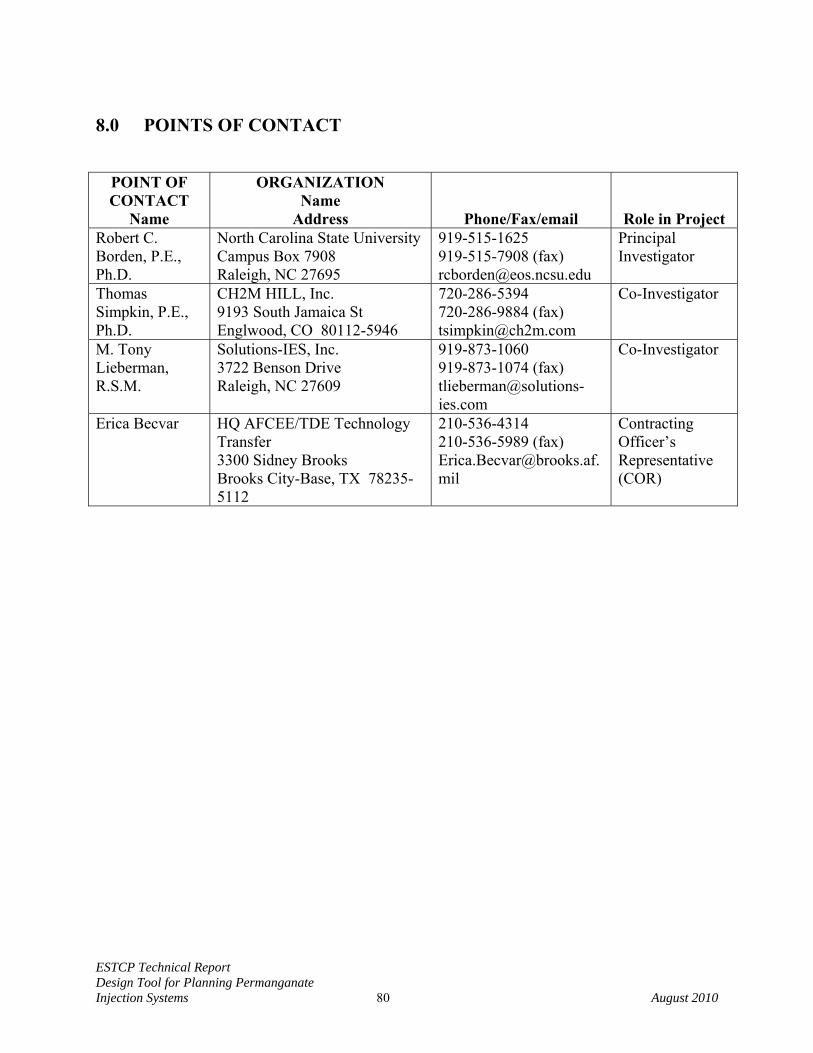
ESTCP Technical Report Design Tool for Planning Permanganate Injection Systems 80 August 2010
8.0 POINTS OF CONTACT
POINT OF CONTACT
Name
ORGANIZATION Name
Address Phone/Fax/email Role in Project Robert C. Borden, P.E., Ph.D.
North Carolina State University Campus Box 7908 Raleigh, NC 27695
919-515-1625 919-515-7908 (fax) [email protected]
Principal Investigator
Thomas Simpkin, P.E., Ph.D.
CH2M HILL, Inc. 9193 South Jamaica St Englwood, CO 80112-5946
720-286-5394 720-286-9884 (fax) [email protected]
Co-Investigator
M. Tony Lieberman, R.S.M.
Solutions-IES, Inc. 3722 Benson Drive Raleigh, NC 27609
919-873-1060 919-873-1074 (fax) [email protected]
Co-Investigator
Erica Becvar HQ AFCEE/TDE Technology Transfer 3300 Sidney Brooks Brooks City-Base, TX 78235-5112
210-536-4314 210-536-5989 (fax) [email protected]
Contracting Officer’s Representative (COR)