Design sensitivity analysis for sequential structural ... · Design sensitivity analysis for...

JOURNAL OFSOUND ANDVIBRATION

www.elsevier.com/locate/jsvi

Journal of Sound and Vibration 263 (2003) 569–591

Design sensitivity analysis for sequentialstructural–acoustic problems

Nam H. Kima, Jun Dongb, Kyung K. Choib,*, N. Vlahopoulosc, Z.-D. Mad,M.P. Castanierd, C. Pierred

aDepartment of Mechanical and Aerospace Engineering, College of Engineering, University of Florida, Gainesville, FL

32611, USAbCenter for Computer-Aided Design, Department of Mechanical Engineering, College of Engineering, The University of

Iowa, Iowa City, IA 52242-1000, USAcDepartment of Naval Architecture and Marine Engineering, The University of Michigan, Ann Arbor, MI 48109, USA

dDepartment of Mechanical Engineering, The University of Michigan, Ann Arbor, MI 48109, USA

Received 29 August 2001; accepted 30 June 2002

Abstract

A design sensitivity analysis of a sequential structural–acoustic problem is presented in which structuraland acoustic behaviors are de-coupled. A frequency-response analysis is used to obtain the dynamicbehavior of an automotive structure, while the boundary element method is used to solve the pressureresponse of an interior, acoustic domain. For the purposes of design sensitivity analysis, a directdifferentiation method and an adjoint variable method are presented. In the adjoint variable method, anadjoint load is obtained from the acoustic boundary element re-analysis, while the adjoint solution iscalculated from the structural dynamic re-analysis. The evaluation of pressure sensitivity only involves anumerical integration process for the structural part. The proposed sensitivity results are compared to finitedifference sensitivity results with excellent agreement.r 2002 Elsevier Science Ltd. All rights reserved.

1. Introduction

Structure-induced noise and vibration control at low frequency is an important area of researchfor reducing the noise level generated by various structural parts. In automotive applications, forexample, the noise level of a passenger compartment can be reduced by changing the structuraldesign parameters. Design sensitivity analysis (DSA) is an essential process in the gradient-based

*Corresponding author. Tel.: +1-319-335-3380; fax: +1-319-335-5669.

E-mail address: [email protected] (K.K. Choi).

0022-460X/03/$ - see front matter r 2002 Elsevier Science Ltd. All rights reserved.

PII: S 0 0 2 2 - 4 6 0 X ( 0 2 ) 0 1 0 6 7 - 2

optimum control technique. Some research results have been reported in DSA of a structural–acoustic problem. Ma and Hagiwara [1, 2], Wang et al. [3], and Choi et al. [4] developed DSA of acoupled structural–acoustic problem using a finite element method (FEM). Either a direct orfrequency method is used to solve the system of matrix equations. However, the excessive numberof elements to represent the complicated three-dimensional acoustic cavity has been the majorbottleneck of the finite element-based approach [5]. To avoid the problems associated with a largenumber of elements in an acoustic domain, Salagame et al. [6] presented an analytical sensitivitymethod using a Rayleigh integral [7]. The sensitivity of a surface velocity is obtained bydifferentiating the frequency-response matrix equation, and the pressure sensitivity is thencalculated by differentiating the Rayleigh integral. This approach is limited to a flat plateproblem. Recently, Scarpa [8] proposed a parametric sensitivity calculation method using asymmetric Eulerian formulation. The velocity potential is used instead of the pressure to representthe fluid’s behavior.

Compared to FEM, the boundary element method (BEM) has an advantage in the modelling ofthe acoustic cavity: It is unnecessary to generate a complicated, three-dimensional acoustic model.Several research studies have been conducted for DSA using BEM. Assuming that the structure’svelocity sensitivity is known, Smith and Bernhard [9] developed a semi-analytical designsensitivity formulation. Cunefare and Koopman [10], Kane et al. [11], Matsumoto et al. [12], andKoo [13] presented an analytical design sensitivity formulation using BEM. For the generalstructure-induced noise problem, however, the velocity sensitivity has to be calculated from thestructural frequency-response analysis [14]. A structural acoustic sensitivity algorithm with respectto sizing design variables based on finite element and boundary element computations has beenpresented [15]. A structural acoustic sensitivity formulation based on boundary elements has beendeveloped for structures subject to stochastic excitation [16].

In this paper, a design sensitivity analysis of a sequential structural–acoustic problem is presentedin which structural and the acoustic behaviors are de-coupled. For the case of a harmonicexcitation, the dynamic behavior of the structure is described using a frequency-response analysis. Aboundary element method [17] is used to calculate the radiated noise (pressure) from the structuralresponse (harmonic velocity). Instead of differentiating a discrete matrix equation, a continuousvariational equation is differentiated with respect to the design parameter. In case of sizing design,the boundary integral equation does not contain any terms that are explicitly dependent on thedesign; only implicitly dependent terms exist through the state variables.

While the direct differentiation method in DSA follows the same solution process as theresponse analysis, the adjoint variable method follows a reverse process. One of the challenges ofthe adjoint variable method in sequential DSA is how to effectively and practically formulate thisreverse process. For example, in the transient response DSA developed by Haug et al. [18], theadjoint problem becomes a terminal-value problem, whereas the original problem is an initial-value problem. Such an opposite solution process in the adjoint problem causes a significantamount of inconvenience and ineffectiveness in DSA. To overcome these difficulties, a sequentialadjoint variable method is presented in which the adjoint load is obtained from boundary elementre-analysis, and the adjoint variable is calculated from structural dynamic re-analysis. So far, noresearch results have been reported in the development of the adjoint variable method in asequential problem. In addition, it is shown that the acoustic adjoint problem still uses the samecoefficient matrix from the direct problem, even if the coefficient matrix is not symmetric.

N.H. Kim et al. / Journal of Sound and Vibration 263 (2003) 569–591570

2. Review of structural–acoustic analysis

2.1. Frequency-response analysis

Consider a structure under dynamic load Fðx; tÞ: The differential equation that governs thebehavior of this hyperbolic system can be written as

ry;ttðx; tÞ þ Cy;tðx; tÞ þ Lyðx; tÞ ¼ Fðx; tÞ; xAOS; t > 0; ð1Þ

where OS is the structure’s domain, yðx; tÞ the displacement, LðxÞ the linear partial differentialoperator, rðxÞ the structural mass density, and CðxÞ the viscous damping effect. The subscribedcomma denotes the derivative with respect to time, i.e., y;t ¼ @y=@t (velocity) and y;tt ¼ @2y=@t2

(acceleration). The initial conditions of the dynamic problem are given by

yðx; 0Þ ¼ y0ðxÞ; y;tðx; 0Þ ¼ y0;tðxÞ; xAOS; ð2Þ

where y0ðxÞ is the initial displacement, and y0;tðxÞ is the initial velocity.For the steady state response, the time-dependent terms from Eq. (1) should be removed. Since

the harmonic load is being considered, Fðx; tÞ can be expressed as

Fðx; tÞ ¼ fðxÞejot; ð3Þ

where fðxÞ is the magnitude of the harmonic load and o is the load frequency, which is considereda constant. In contrast, the steady state response has the same frequency as the applied load butmay have a different phase angle. Using the complex variable method, the displacement yðx; tÞ canbe expressed as

yðx; tÞ ¼ zðxÞejot; ð4Þ

where zðxÞ is the complex displacement.Time dependency of the dynamic problem can be eliminated by substituting Eqs. (3) and (4)

into Eq. (1), to obtain the spatial state operator equation as

�o2rzðxÞ þ joCzðxÞ þ LzðxÞ ¼ fðxÞ; xAOS ð5Þ

with its appropriate boundary conditions.The variational formulation of Eq. (5) is similar to the static problem. However, since the

complex variable zðxÞ is used for the state variable, the complex conjugate %z� is used for thedisplacement variation. By multiplying %z� and integrating it over the domain OS; the variationalequation can be derived after integration by parts for differential operator L asZ Z

OS

½�o2rzT þ joCzT�%z� dOS þZ Z

OS

rðzÞTeð%z�Þ dOS

¼Z Z

OS

fbT

%z� dOS þZGs

fsT %z� dG; 8%zAZ; ð6Þ

where %z� is the complex conjugate of the kinematically admissible virtual displacement %z; and Z isthe complex space of kinematically admissible virtual displacements. Eq. (6) provides thevariational equation of the dynamic frequency response under an oscillating excitation with

N.H. Kim et al. / Journal of Sound and Vibration 263 (2003) 569–591 571

frequency o. For derivational convenience, the following terms are defined:

duðz; %zÞ ¼Z Z

OS

rzT%z� dOS; ð7Þ

cuðz; %zÞ ¼Z Z

OS

CzT%z� dOS; ð8Þ

auðz; %zÞ ¼Z Z

OS

rðzÞTeð%z�Þ dOS; ð9Þ

cuð%zÞ ¼Z Z

OS

fbT

%z� dOS þZGs

fsT %z� dG; ð10Þ

where du(,) is the kinetic sesqui-linear form, cu(,) is the damping sesqui-linear form, au(,) isthe structural sesqui-linear form, and cuðÞ is the load semi-linear form. The definitions of thesesqui-linear and semi-linear forms can be found in Ref. [19].

Since the structure-induced pressure within the acoustic domain is related to the velocityresponse, it is convenient to transfer displacement to velocity using the relation

vðxÞ ¼ jozðxÞ: ð11Þ

By using Eqs. (6)–(11), the variational equation of the frequency-response problem can beobtained as

joduðv; %zÞ þ cuðv; %zÞ þ1

joauðv; %zÞ ¼ cuð%zÞ; 8%zAZ: ð12Þ

The structural damping, a variant of viscous damping, is caused either by internal materialfriction or by the connection between structural components. It has been experimentally observedthat for each cycle of vibration the dissipated energy of the material is proportional todisplacement [20]. When the damping coefficient is small, as in the case of structures, damping isprimarily effective at those frequencies close to the resonance. The variational equation with thestructural damping effect is

joduðv; %zÞ þ kauðv; %zÞ ¼ cuð%zÞ; 8%zAZ; ð13Þ

where k ¼ ð1þ jfÞ=jo; and f is the structural damping coefficient.After the structure is approximated using finite elements, and kinematic boundary conditions

are applied, the following system of matrix equations is obtained:

½joMþ kK�fvðoÞg ¼ ffðoÞg; ð14Þ

where ½M� is the mass matrix and ½K� is the stiffness matrix.

2.2. Acoustic boundary element method

From the structure’s velocity result, the boundary element method is used to evaluate thepressure response in an acoustic domain. The standard wave equation is reduced to the Helmholtzequation [21] in the harmonic response problem as

r2p þ k2p ¼ 0; ð15Þ


where p is the pressure, kð¼ o=cÞ is the wave number, c is the velocity of the wave propagation,and r2 is the Laplace operator.

For BEM, the structural behavior must first be computed, and then it can be used as aboundary condition to compute radiated noise p: If the acoustic domain is considered to be in R3;then the boundary of this domain constitutes the structure’s domain, OS: By integrating over thedomain and by using Green’s theorem, the Helmholtz equation (15) constitutes the boundaryintegral equation [21] as Z Z

OS

Gðx;x0Þ@p

@n� pðxÞ

@G

@n

� �dOS ¼ apðx0Þ; ð16Þ

where Gðx;x0Þ is Green’s function, x is the position of a reference point, x0 is the position of anobservation point, @=@n is the normal component of the gradient, and S is the acoustic boundary,which is again a structural domain. In Eq. (16), the constant a is equal to 1 for x0 inside theacoustic volume, 0.5 for x0 on a smooth boundary surface, and 0 for x0 outside the acousticvolume. Note that Eq. (16) can provide a solution for both radiation and interior acousticproblems.

On the surface of the acoustic boundary, the following relation between the pressure and thestructural velocity is given:

rp ¼ �jrov; ð17Þ

where r is the structural density and v is the acoustic velocity, which was computed from thefrequency response in Eq. (13). If xS is a point on the acoustic boundary surface, then theboundary integral equation (16) becomesZ Z

OS

�jroGðxS; x0ÞvnðxSÞ �@G

@npðxSÞ

� �dOS ¼ apðx0Þ; ð18Þ

where vn is the normal component of surface velocity v: For derivational convenience, Eq. (18) canbe rewritten as

bðv0; vÞ þ eðx0; pSÞ ¼ apðx0Þ; ð19Þ

where bðx0;Þ and eðx0;Þ are linear integral forms that correspond to the left-hand side ofEq. (18). Note that unlike the structural forms in Eqs. (7)–(10), these integral forms areindependent of the sizing design variable; thus no subscribed u is used in their definitions.

The boundary element method has two steps: first evaluating the pressure variable on theacoustic boundary using the structural velocity, and then calculating the pressure variable withinthe acoustic domain using the boundary pressure information. Let the acoustic boundary S beapproximated by N number of nodes. If observation point x0 is positioned at every node, then thefollowing linear system of equations is obtained:

½A�fpSg ¼ ½B�fvg; ð20Þ

where fpSg ¼ fp1; p2;y; pNgT is the nodal pressure vector, fvg is the 3N � 1 velocity vector, ½A� is

the N � N coefficient matrix, and [B] is the N � 3N coefficient matrix. Note that these vectors andmatrices are all complex variables. The process of computing the boundary pressure fpSg assumesdomain discretization, and the condition in Eq. (19) is imposed in every node. However, for the


purposes of DSA, let us consider a continuous counterpart to Eq. (20), defined as

AðpSÞ ¼ BðvÞ; ð21Þ

where the integral forms A() and B() correspond to the matrices ½A� and ½B� in Eq. (20),respectively. The boundary pressure can then be calculated from pS ¼ A�1

3BðvÞ .Once {pS} has been computed, Eq. (19) can be used to compute the acoustic pressure at any

point x0 within the acoustic domain in the form of a vector equation as

pðx0Þ ¼ fbðx0ÞgTfvg þ feðx0Þg

TfpSg; ð22Þ

where {b(x0)} and {e(x0)} are the column vectors that correspond to the left-hand side of theboundary integral equation (18).

In a sizing design problem, in which panel thickness is a design variable, integral forms bðx0;Þand eðx0;Þ in Eq. (19) are independent of the design variable. Only implicit dependence on thedesign exists through the state variable v and p; which will be developed in the following section.However, in a shape design problem, the acoustic domain changes according to the structuraldomain change, which is a design variable. Thus, integral forms bðx0;Þ and eðx0;Þ depend onthe design. Such a problem, however, is not investigated in this study.

3. Design sensitivity analysis

The purpose of design sensitivity analysis (DSA) is to compute the dependency of performancemeasures on the design. In this study, only sizing design is considered, such as the thickness of aplate and the cross-sectional dimension of a beam.

3.1. Design sensitivity formulas

Assume that cðuÞ is continuously differentiable with respect to design u. If the design isperturbed in the direction of du (arbitrary), and t is a parameter that controls the perturbationsize, then the variation of cðuÞ in the direction of du is defined as

c0du �

d

dtcðuþ tduÞ

��t¼0

¼@cT

@udu: ð23Þ

Throughout this paper, prime ‘‘ 0 ’’ plays precisely the same role as the first variation in thecalculus of variations. For convenience, subscribed du will often be ignored. The term‘‘derivative’’ or ‘‘differentiation’’ will often be used to denote the variation in Eq. (23). If thevariation of a function is continuous and linear with respect to du; the function is differentiable(even more precisely, it is Fr!echet differentiable).

It is also assumed that the solution to the frequency-response problem in Eq. (13) and thesolution to the boundary integral equation (19) are differentiable with respect to the design. Thatis, the following forms of variation exist:

v0 ¼d

dt½vðx; uþ tduÞ�

��t¼0

¼@v

@udu ð24Þ


and

p0 ¼d

dt½pðx; uþ tduÞ�

��t¼0

¼@pT

@udu: ð25Þ

3.2. Direct differentiation method

A direct differentiation method computes the variation of state variables in Eqs. (24) and (25)by differentiating the state equations (13) and (19) with respect to the design. Let us first considerthe structural part, i.e., the frequency-response analysis in Eq. (13). The forms that appear inEq. (13) explicitly depend on the design, and their variations are defined as

d 0duðv; %zÞ �

d

dt½duþtduð*v; %zÞ�

��t¼0

; ð26Þ

a0duðv; %zÞ �

d

dt½auþtduð*v; %zÞ�

��t¼0

ð27Þ

and

c0duð%zÞ �d

dt½cuþtduð%zÞ�

��t¼0

; ð28Þ

where *v denotes state variable v with the dependence on t being suppressed, and %z and its complexconjugate are independent of the design. The detailed expressions of d 0

duð;Þ; a0duð;Þ; and c0duðdÞwill be developed in Section 3.3 using analytical examples.

Thus, by taking a variation of both sides of Eq. (13) with respect to the design, and by movingterms explicitly dependent on the design to the right side, the following sensitivity equation can beobtained:

joduðv0; %zÞ þ kauðv0; %zÞ ¼ c0duð%zÞ � jod 0duðv; %zÞ � ka0

duðv; %zÞ; 8%zAZ: ð29Þ

Presuming that velocity v is given as a solution to Eq. (13), Eq. (29) is a variational equation, withthe same sesqui-linear forms for displacement variation v0: Note that the stiffness matricescorresponding to Eqs. (13) and (29) are the same, and that the right-hand side of Eq. (29) can beconsidered a fictitious load term. If a design perturbation du is defined, and if the right-hand sideof Eq. (29) is evaluated with the solution to Eq. (13), then Eq. (29) can be numerically solved toobtain v0 using the finite element method. By interpreting the right-hand side of Eq. (29) asanother load form, Eq. (29) can be solved by using the same solution process as the frequency-response problem in Eq. (13).

Now the acoustic aspect will be considered, which is represented by the boundary integralequation (19). A direct differentiation of Eq. (19) yields the following sensitivity equation:

bðx0; v0Þ þ eðx0; p

0SÞ ¼ ap0ðx0Þ: ð30Þ

Since integral forms bðx0;Þ and eðx0;Þ are independent of the design, the above equation hasexactly the same form as Eq. (19). Thus, using the solution (v0) of the structural sensitivityequation (29), Eq. (30) can be used by following the same solution process as BEM, to obtain thepressure sensitivity result. Thus, like Eq. (20), the following matrix equation has to be solved in


the discrete system:

½A�fp0Sg ¼ ½B�fv0g: ð31Þ

Then, like Eq. (22), the pressure sensitivity at point x0 can be obtained from

p0ðx0Þ ¼ fbðx0ÞgTfv0g þ feðx0Þg

Tfp0Sg: ð32Þ

This sensitivity calculation process is the same as the BEM solution process described fromEq. (20) to Eq. (22).

3.2.1. Structural performance measureA general performance measure that represents a variety of structural responses can be written

in integral form as

c1 ¼Z Z

OS

gðv; uÞ dOS: ð33Þ

where function gðv; uÞ is assumed to be continuously differentiable with respect to its arguments.The integral form of a performance measure in the above equation is not restricted in representinga general function. For example, if a function value at a point is required, then a Dirac-deltameasure may be used inside the integration. The reason for introducing the integral form of aperformance measure is that in FEM the pointwise definition of a function is meaningless, sincethe variational formulation enforces the definition of a function value in the sense of a Sobolevnorm [22]. This is different from BEM, in which a function can be defined at a point. Note that c1

is a complex functional in frequency-response analysis.The variation of c1 with respect to the design variable becomes

c01 ¼

d

dt

Z ZOS

gðvðx; uþ tduÞ; uþ tduÞdOS

� ��t¼0

¼Z Z

OS

ðgT;vv

0 þ gT;uduÞ dO

S; ð34Þ

where g;v ¼ @g=@v and g;u ¼ @g=@u are column vectors, and their expressions are known from thedefinition of the function g: The objective of DSA is to obtain an explicit expression of c0

1 in termsof du: If the structural design sensitivity equation (29) is solved for the variation v0; then thesensitivity of c1 can be calculated from Eq. (34) using the numerical integration process.

3.2.2. Acoustic performance measure

Consider a performance measure that is defined at point x0 within the acoustic domain as

c2ðx0Þ ¼ h pðx0Þ; uð Þ; ð35Þ

where the function hðp; uÞ is assumed to be continuously differentiable with respect to itsarguments. Note that acoustic performance c2 is not defined in the integral form, as was the casefor structural performance c1:


The variation of the performance measure with respect to the design variable becomes

c02 ¼

d

dt½hðpðx; uþ tduÞ; uþ tduÞ�

��t¼0

¼ h;pp0 þ hT;udu; ð36Þ

where the expression of h;p ¼ @h=@p and h;u ¼ @h=@u are known from the definition of the functionh: Thus, from the solution to the acoustic design sensitivity equation (30), the sensitivity of c2 canreadily be calculated. However, the calculation of p0 also requires the solution to the structuralsensitivity equation (29).

3.3. Adjoint variable method

Since the number of design variables is larger than the number of active constraints in manyoptimization problems, the adjoint variable method is attractive [18]. However, the adjointvariable method is known to be limited to a symmetric operator problem. In this section, theadjoint variable method is further extended to non-symmetric complex operator problems. Sincethe adjoint variable method is directly related to the performance measure, structural and acousticperformance measures are treated separately. In case of an acoustic performance measure, asequential adjoint variable method is introduced.

3.3.1. Structural performance measureTo obtain an explicit expression for c0

1 in terms of du; it is necessary to rewrite the first term inEq. (34) explicitly in terms of du: As with the static problem, an adjoint equation can beintroduced by replacing v0 in Eq. (34) with the complex virtual displacement %k and by equating itto the variational equation (13) with respect to adjoint variable kn as

joduð %k;kÞ þ kauð %k; kÞ ¼Z Z

OS

gT;v%k dOS; 8 %kAZ; ð37Þ

where an adjoint solution, kAZ , or equivalently its complex conjugate kn; is desired. Note thatthe forms duð;Þ and auð;Þ are not symmetric with respect to their arguments, because theirarguments are complex variables. Since Eq. (37) is satisfied for all %kAZ; and since v0AZ; Eq. (37)may be evaluated at %k ¼ v0; to obtain

joduðv0; kÞ þ kauðv0; kÞ ¼Z Z

OS

gT;vv

0 dOS: ð38Þ

In addition, since the sensitivity equation (29) is satisfied for all %zAZ; and since kAZ; Eq. (29) maybe evaluated at %z ¼ k to obtain

joduðv0;kÞ þ kauðv0; kÞ ¼ c0duðkÞ � jod 0duðv;kÞ � ka0

duðv;kÞ: ð39Þ

It becomes apparent that the left-hand side of Eqs. (38) and (39) are exactly the same. Thus, fromthese two equations we obtainZ Z

OS

gT;vv

0 dOS ¼ c0duðkÞ � jod 0duðv; kÞ � ka0

duðv; kÞ: ð40Þ


Therefore, the terms that are implicitly dependent on the design in Eq. (34) are explicitly expressedin terms of du: By substituting the relation in Eq. (40) into Eq. (34), c0 is explicitly represented interms of du as

c01 ¼

Z ZOS

gT;udu dOS þ c0duðkÞ � jod 0

duðv; kÞ � ka0duðv; kÞ: ð41Þ

Specific expressions of c0 for different performance measures and different structural componentswill be developed in detail in the analytical example section.

3.3.2. Acoustic performance measureThe acoustic performance c2 in Eq. (35) is defined at point x0; and its sensitivity expression in

Eq. (36) contains p0; which has to be explicitly expressed in terms of du: The objective is to expressp0 in terms of v0 such that the adjoint problem defined in the previous section can be used. Bysubstituting the relation in Eq. (30) into the sensitivity expression of Eq. (36), and by using therelation in Eq. (21), we obtain

c02 ¼ hT

;uduþ h;pp0

¼ hT;uduþ h;p½bðx0; v

0Þ þ eðx0;A�13Bðv0ÞÞ�: ð42Þ

In Eq. (42), a ¼ 1 is used since x0 is the interior point. Thus, c02 is expressed in terms of v0: The

second term on the right-hand side of the above equation can be used to define the adjoint load bysubstituting %k for v0: Hence, the following form of the adjoint problem is obtained:

joduð %k;kÞ þ kauð %k;kÞ ¼ h;p½bðx0; %kÞ þ eðx0;A�13Bð %kÞÞ�; 8 %kAZ; ð43Þ

where an adjoint solution kn is desired. By following the same process that is described fromEqs. (37) to (41), the sensitivity of c2 can be obtained as

c02 ¼ h;uduþ c0duðkÞ � jod 0

duðv;kÞ � ka0duðv;kÞ: ð44Þ

It is interesting to note that even if c2 is a function of pressure p; its sensitivity expression inEq. (44) does not require the value of p; only the structural solution v and the adjoint solution kn

are required in the calculation of c02:

Even if Eq. (44) looks similar to the structural performance measure in Eq. (41), a fundamentaldifference exists in the calculation of the adjoint load in Eq. (43). To illustrate, consider a discreteform of the adjoint load. Eq. (43) can be written in the discrete system as

joMþ kK½ �fk�g ¼ fbg þ ½B�T½A��Tfeg; ð45Þ

where the right-hand side corresponds to the adjoint load in the discrete system. Instead ofcomputing the inverse matrix, let us define an acoustic adjoint problem in BEM as

½A�Tfgg ¼ feg; ð46Þ

where the acoustic adjoint solution {g} is desired. Even if the coefficient matrix [A] is notsymmetric, the adjoint equation (46) can still use the factorized matrix of the boundaryelement equation (20). By substituting {g} into Eq. (45), we obtain the structural adjointproblem, as

½joMþ kK�fk�g ¼ fbg þ ½B�Tfgg: ð47Þ


Note that the acoustic adjoint solution {g}, which is obtained from BEM, is required to computethe structural adjoint load, and frequency-response re-analysis then provides the structuraladjoint solution fkng . Thus, two different adjoint problems are defined: the first is similar toBEM, and is used to compute the adjoint load, while the second is similar to the structuralfrequency-response problem.

3.4. Analytical examples

In many structural–acoustic problems, a structural part is described by using a plate/shellcomponent, and an acoustic domain is enclosed by the structure. A typical design problem wouldreduce sound pressure levels in the passenger position by changing the plate thickness. In such aproblem, the design variable is the thickness of a plate/shell component, and the performancemeasure is the sound pressure level at selected points in the acoustic domain. Also, in order toreduce the radiated acoustic power from the structure, the structure’s velocity can be alsoconsidered as a performance measure.

The structural variational equation of harmonic motion is given by Eq. (13). The objective is toderive explicit forms of duð;Þ; auð;Þ; and cuðÞ for a plate/shell component. In general, ashear-deformable plate/shell has three translation degrees of freedom and two rotational degreesof freedom. Thus, the structural state variable z is defined by

z ¼ ½z1; z2; z3; y1; y2�T: ð48Þ

Strain is decomposed into membrane, bending, and transverse shear parts as

em ¼

z1;1

z2;2

z1;2 þ z2;1

264

375; j ¼

y1;1y2;2

y1;2 þ y2;1

264

375; c ¼

z3;2 � y2z3;1 � y1

" #: ð49Þ

Note that the strain resultants given in Eq. (49) have the following properties: y1;1 is thecurvature in the x1 direction, y2;2 is the curvature in the x2 direction, and ðy1;2 þ y2;1Þ is thetwisting curvature. In Eq. (49), z3;2 � y2 and z3;1 � y1 are the shear rotation in the 2�3 and 1�3plane, respectively. By using the above definitions, the structural sesqui-linear form [23] isdefined as

auðz; %zÞ ¼Z Z

OS

½hemð%z�ÞTCemðzÞ þh3

12jð%z�ÞTCjðzÞ þ hcð%z�ÞTDcðzÞ� dOS; ð50Þ

where

C ¼E

1� n2

1 n 0

n 1 0

0 0 ð1� nÞ=2

264

375; D ¼

Ex2ð1þ nÞ

1 0

0 1

" #; ð51Þ

and x is the shear correction factor, compensating for the assumption of constant shear strainalong the cross-section. The three terms within the integral of Eq. (50) represent the membrane,bending, and transverse shear contribution. Since a0

duð;Þ is the explicit derivative of auð;Þ


with respect to h;

a0duðz; %zÞ ¼Z Z

OS

½emð%z�ÞTCemðzÞ þh2

4jð%z�ÞTCjðzÞ þ gð%z�ÞTDcðzÞ�dh dOS: ð52Þ

From the known structural solution z (or v), the structural variation of Eq. (52) can be calculatedusing the numerical integration process.

For plate/shell components, the kinetic sesqui-linear form and its variation can bedefined as

duðz; %zÞ ¼Z Z

OS

rhzT%z� dOS ð53Þ

and

d 0duðz; %zÞ ¼

Z ZOS

ðrzT%z�Þdh dOS: ð54Þ

If the applied load consists of externally applied pressure F(x) and the self-weight given by

fðxÞ ¼ FðxÞ þ gghðxÞ; ð55Þ

where g is the weight density of the plate, and g is a unit vector in the direction of gravity, then theload semi-linear form cuðÞ and its variation can be defined as

cuð%zÞ ¼Z Z

OS

½Fþ ggh�T%z� dOS ð56Þ

and

c0duð%zÞ ¼Z Z

OS

ggT%z�dh dOS: ð57Þ

1N 1N

1N1N

(0,0,3)

(0,1.2,0)

(1,0,0)0

A1, S1

A2

S2

Rigid Walls

Flexible Panel

x2

x1

x3

Fig. 1. Acoustic cavity with flexible wall.


Consider an acoustic cavity with a flexible panel, as illustrated in Fig. 1. The cavity issurrounded on all but one side by rigid walls, and the open side is closed by a clamped panel oflinear elastic material with the structural damping coefficient j: The panel’s uniform thickness, h;is selected as the design variable, i.e., uðxÞ ¼ fhg: Let us consider such performance measures asthe acoustic pressure pðxaÞ at point xa in the acoustic cavity, and the x3 directional velocity v3ðxsÞat point xs on the structural panel. A harmonic force f ðx; tÞ with frequency o is applied to theplate. Here, f ðx; tÞ is assumed to be independent of the design variable u(x).

3.4.1. Structural performance measureThe performance measure in this example is the vertical velocity at point x

s, whosemathematical expression is

c1 ¼ v3ðxsÞ ¼Z Z

OS

dðx� xsÞv3 dOS; ð58Þ

where dðÞ is the Dirac-delta measure at zero. Eq. (58) is a simple form of Eq. (33), which is thegeneral form for a structural performance measure. The variation of c1 is

c01 ¼ v03ðx

sÞ ¼Z Z

OS

dðx� xsÞv03 dOS: ð59Þ

Working from Eq. (37), the corresponding adjoint equation is obtained as

joduð %k;kÞ þ kauð %k; kÞ ¼Z Z

OS

dðx� xsÞ %k3 dOS; 8 %kAZ: ð60Þ

In Eq. (60), the term on the right-hand side is the adjoint load for the structural velocity.The physical meaning of the adjoint load, which corresponds to the harmonic velocity at apoint, is a unit harmonic force applied at point xs: The design sensitivity of c1 is obtained fromEq. (41) as

c01 ¼ c0duðkÞ � jod 0


The fact that the primary state equation (13) and the adjoint equation (60) represent the samestructure with different loads provides an efficient method for numerical implementation, sinceonly one finite element model is required to solve both the original and adjoint equations.Substituting the variations of those forms in Eqs. (52), (54), and (57), the design sensitivityexpression becomes

c01 ¼

Z ZOS

ggTk�dh dOS � joZ Z

OS

ðrvTk�Þdh dOS

� kZ Z

OS

½emðk�ÞTCemðvÞ þh2

4jðk�ÞTCjðvÞ þ cðk�ÞTDcðvÞ�dh dOS: ð62Þ

Thus, c0

1 is expressed in terms of dh:

3.4.2. Acoustic performance measure

Consider a pressure performance measure at point xa; given as

c2 ¼ pðxaÞ: ð63Þ


Eq. (63) is a simple form of Eq. (35), a general form of the acoustic performance measure. Thevariation of the performance measure, corresponding to Eq. (42), is

c02 ¼ p0ðxaÞ ¼ bðxa; v0Þ þ eðxa;A�1

3Bðv0ÞÞ: ð64Þ

The adjoint equation for c02 is obtained using Eq. (43) as

joduð %k;kÞ þ kauð %k; kÞ ¼ bðxa; %kÞ þ eðxa;A�13Bð %kÞÞ; 8 %kAZ: ð65Þ

The term on the right-hand side of this equation is referred to as the acoustic adjoint load. Inactual implementation, the adjoint load is calculated from the secondary adjoint problem definedin Eq. (46). The discrete adjoint problem in Eq. (47) can then be solved for k*. From Eq. (41), thedesign sensitivity expression of the acoustic pressure becomes

c02 ¼ c0duðkÞ � jod 0


Note that the design sensitivity expression in Eqs. (61) and (66) has identical forms. Thus, thesame numerical integration process can be used for both structural and acoustic performancemeasures. However, in case of an acoustic performance measure, the secondary adjoint problemin Eq. (46) must be solved in order to define the structural adjoint load.

4. Numerical examples

4.1. Numerical method

A structural–acoustic system is solved using both finite element and the boundary elementmethods. The variational equation of the harmonic motion of a continuum model, Eq. (13), canbe reduced to a set of linear algebraic equations by discretizing the model into elements and byintroducing shape functions and nodal variables for each element. It is assumed that the structuralfinite element and the acoustic boundary element meshes match at their interfaces. Acousticpressure pðxÞ and structural velocity vðxÞ are approximated using shape functions and nodalvariables for each element in the discretized model as

vðxÞ ¼ NsðxÞve

pðxÞ ¼ NaðxÞpe

); ð67Þ

where NsðxÞ and NaðxÞ are matrices of shape functions for velocity and pressure, respectively, andve and pe are the element nodal variable vectors. Substituting Eq. (67) into Eq. (13) and carryingout integration yields the same matrix equation as Eq. (14) rewritten here as

½joMþ kK�fvðoÞg ¼ ffðoÞg: ð68Þ

After obtaining the structural velocity, BEM is used to evaluate the pressure response on theboundary, as well as within the acoustic domain, as explained in Section 2.2.

Fig. 2 shows the computational procedure for the adjoint variable method with a structuralFEA and an acoustic BEA code. Even if FEM and BEM are used to evaluate the acousticperformance measure, only the structural response v is required to perform design sensitivityanalysis. The adjoint load is calculated from the transposed boundary element analysis, and the


adjoint equations are then numerically solved using the FEA code with the same finite elementmodel used for the original structural analysis.

Numerical solutions are used to compute the design sensitivity, and the integration of the designsensitivity expressions in Eq. (44) can be evaluated using a numerical integration method, such asthe Gauss quadrature method [23]. The integrands are functions of the state variable, the adjointvariable, and gradients of both variables, as illustrated in Eq. (44).

4.2. Design sensitivity analysis of a box model

Fig. 3 depicts the acoustic cavity and the panel, previously discussed in Section 3.3. Theacoustic medium in the cavity is air, with a mass density of r0 ¼ 1:205 kg/m3 and wave

Fig. 3. An acoustic box model.

Structural ModelingDesign Parameterization

Structural FEA[jωM + κK]{v(ω)} = {f(ω)}

Acoustic BEA[A]{pS} = [B]{v}

p = {b}T{v} + {e}T{pS}

Acoustic Adjoint Problem (BEM)[A]T{ } = {e}

Structural Adjoint Problem (FEM)[jωM + κK]{ *} = {b}+[B]T{ }

Sensitivity Computation( , ) ( )

( , ) ( , )j d aδ

δ δ

ψω κ

′ ′=′ ′− −

u

u u

v � �

�

� �

�

�v v

l

Fig. 2. Computational procedure of design sensitivity analysis.


propagation velocity of c ¼ 344m/s. The panel is an aluminum plate with thickness of 0.01m,mass density of rs ¼ 2700 kg/m3, Young’s modulus of E ¼ 7:1� 1010 Pa, a Poisson’s ratio ofn ¼ 0:334; and a structural-damping coefficient of j ¼ 0:06: A harmonic force f ¼ 1:0 N in the x3

direction is applied at four points on the plate as shown in Fig. 1. The whole structure isdiscretized by 864 elements and 866 nodes. In the frequency-response analysis, the five sides of thestructure are fixed to simulate the rigid wall; only the bottom panel is allowed to move. In theacoustic analysis, the pressure value of each node is calculated from the structural velocity dataand the pressure value in the acoustic cavity is then evaluated.

Panel thickness is chosen as the design variable, and only one design variable is considered inthis example. The following design sensitivities are considered: the acoustic pressure at A1

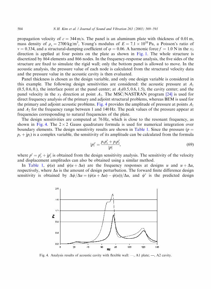
ð0:5; 0:6; 0:Þ; the interface point at the panel center; at A2ð0:5; 0:6; 1:5Þ; the cavity center; and thepanel velocity in the x3 direction at point A1: The MSC/NASTRAN program [24] is used fordirect frequency analysis of the primary and adjoint structural problems, whereas BEM is used forthe primary and adjoint acoustic problems. Fig. 4 provides the amplitude of pressure at points A1

and A2 for the frequency range between 1 and 140Hz. The peak values of the pressure appear atfrequencies corresponding to natural frequencies of the plate.

The design sensitivities are computed at 76Hz, which is close to the resonant frequency, asshown in Fig. 4. The 2� 2 Gauss quadrature formula is used for numerical integration overboundary elements. The design sensitivity results are shown in Table 1. Since the pressure ðp ¼pr þ jpiÞ is a complex variable, the sensitivity of its amplitude can be calculated from the formula

jpj0 ¼prp

0r þ pip

0i

jpj; ð69Þ

where p0 ¼ p0r þ jp0i is obtained from the design sensitivity analysis. The sensitivity of the velocity

and displacement amplitudes can also be obtained using a similar method.In Table 1, cðuÞ and cðu þ DuÞ are the frequency responses at designs u and u þ Du;

respectively, where Du is the amount of design perturbation. The forward finite difference designsensitivity is obtained by Dc=Du ¼ ðcðu þ DuÞ � cðuÞÞ=Du; and c0 is the predicted design

Fig. 4. Analysis results of acoustic cavity with flexible wall: —, A1 plate; —, A2 cavity.


sensitivity using the proposed method. A design perturbation of Du ¼ 1:0� 10�6 m is used, andthe predicted values are compared with the finite difference results. Table 1 presents designsensitivity results for the acoustic pressure, in Pascal (Pa), and for the structural velocity in the x3

direction. Good agreement is obtained between c0 and Dc=Du: Since the applied load magnitudeis fixed, an increase in panel thickness reduces plate vibration and radiated pressure.Consequently, all sensitivities are negative.

A major advantage of the adjoint variable method appears when a large number of designvariables exist. In the early product development stage, for example, a design engineer may wantto decide on the panel thickness for each section in order to minimize acoustic noise. To this end,the element sensitivity plot (Fig. 5) clearly shows the sensitivity of the pressure at the cavity centerto the elements, and helps to determine new panel thicknesses. If the direct differentiation methodis employed, then 144 design sensitivity equations must be solved in order to obtain suchinformation, while with the adjoint variable method only one adjoint equation needs to be solved.

4.3. Design sensitivity analysis of a vehicle model

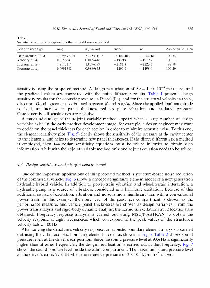
One of the important applications of this proposed method is structure-borne noise reductionof the commercial vehicle. Fig. 6 shows a concept design finite element model of a next generationhydraulic hybrid vehicle. In addition to power-train vibration and wheel/terrain interaction, ahydraulic pump is a source of vibration, considered as a harmonic excitation. Because of thisadditional source of excitation, vibration and noise is more significant than with a conventionalpower train. In this example, the noise level of the passenger compartment is chosen as theperformance measure, and vehicle panel thicknesses are chosen as design variables. From thepower train analysis and rigid-body dynamic analysis, the harmonic excitations at 12 locations areobtained. Frequency-response analysis is carried out using MSC/NASTRAN to obtain thevelocity response at eight frequencies, which correspond to the peak values of the structure’svelocity below 100Hz.

After solving the structure’s velocity response, an acoustic boundary element analysis is carriedout using the cabin acoustic boundary element model, as shown in Fig. 6. Table 2 shows soundpressure levels at the driver’s ear position. Since the sound pressure level at 93.6Hz is significantlyhigher than at other frequencies, the design modification is carried out at that frequency. Fig. 7shows the sound pressure level inside the cabin compartment. The maximum sound pressure levelat the driver’s ear is 77.8 dB when the reference pressure of 2� 10–8 kg/mms2 is used.

Table 1

Sensitivity accuracy compared to the finite difference method

Performance type cðuÞ cðu þ DuÞ DcDu c0 Dc=Du=c0�100%

Displacement at A1 3.27959E�5 3.27557E�5 �0.040403 �0.040181 100.55

Velocity at A1 0.015668 0.0156416 �19.219 �19.187 100.17

Pressure at A1 1.8118117 1.8096199 �2191.8 �2223.3 98.58

Pressure at A2 0.9901643 0.9889635 �1200.8 �1198.4 100.20


Forty design variables are selected in this example. First, the acoustic adjoint problem inEq. (46) is solved, and the structural adjoint problem of Eq. (47) is then solved to obtain theadjoint response k*. Using the velocity response v and the adjoint response k*, the numericalintegration process given in Eq. (66) calculates the sensitivity results for each structural panel, asshown in Table 3. The results show that a thickness change in the chassis component has thegreatest potential for achieving a reduction in sound pressure levels. Since the numericalintegration process is carried out on each finite element, the element sensitivity information can becalculated without any additional effort. Fig. 8 plots the sensitivity contribution of each elementto the sound pressure level. Such graphic-based sensitivity information is very helpful to thedesign engineer to determine the direction of the design modification.

Fig. 5. (Negative of) element sensitivity for the pressure at the cavity center.


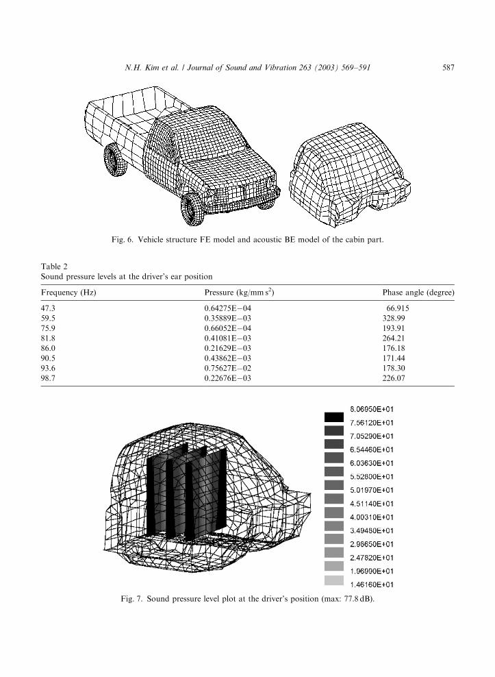
Fig. 6. Vehicle structure FE model and acoustic BE model of the cabin part.

Table 2

Sound pressure levels at the driver’s ear position

Frequency (Hz) Pressure (kg/mm s2) Phase angle (degree)

47.3 0.64275E�04 66.915

59.5 0.35889E�03 328.99

75.9 0.66052E�04 193.91

81.8 0.41081E�03 264.21

86.0 0.21629E�03 176.18

90.5 0.43862E�03 171.44

93.6 0.75627E�02 178.30

98.7 0.22676E�03 226.07

Fig. 7. Sound pressure level plot at the driver’s position (max: 77.8 dB).


In Table 4, the accuracy of the proposed sensitivity result is compared to the sensitivity resultcalculated using the finite difference method. The vertical velocity at the center of the cabin roof isconsidered as a performance measure. The proposed sensitivity results agreed with the finitedifference sensitivity results within a range of 10% when 0.1% of the thickness is perturbed.

As was shown in Table 3, the chassis component has the highest sensitivity for the soundpressure level, which means that a change in the thickness of the chassis component is the

Fig. 8. Element design sensitivity plot with respect to panel thickness.

Table 3

Normalized sound pressure level sensitivity w.r.t. panel thickness

Component Sensitivity Component Sensitivity

Chassis �1.0 Chassis MTG �0.11

Left wheelhouse �0.82 Chassis connectors �0.10

Right door 0.73 Right fender �0.07

Cabin �0.35 Left door �0.06

Right wheelhouse �0.25 Bumper �0.03

Bed �0.19 Rear glass 0.03


most effective way to reduce the sound pressure level. The thickness of the chassis is there-fore increased by 1.0mm.The whole analysis process is repeated for the modified design.Fig. 9 shows sound pressure levels at the driver’s ear when the excitation frequency is93.6Hz at the updated design. The maximum value of the sound pressure is reduced from 77.8to 75.0 dB.

Structural–acoustic performance improvement at the updated design can be investigatedfurther by considering the pressure results around the critical frequency. Fig. 10 plots thechange in the level of sound pressure at the driver’s ear for the initial and improved design.

Table 4

Design sensitivity result for vz at the cabin roof center (initial value=0.40293mm/s, perturbation=0.1%)

Design Perturbed FDM DSA Ratio (%)

Bumper 0.40292 �3.5739E�3 �3.9091E�3 91.43

Chassis 0.40196 �3.1287E�1 �3.0824E�1 101.50

Arm LL 0.40288 �9.8022E�3 �9.6368E�3 101.72

Arm LR 0.40250 �9.0502E�2 �9.6967E�2 93.33

Oil Box 0.40293 1.9519E�3 2.0538E�3 95.04

Brake FL 0.40289 �6.9373E�3 �6.4794E�3 107.07

Brake FR 0.40239 �1.0890E�1 �9.7718E�2 111.45

Chassis Conn 0.40274 �5.2836E�2 �5.2732E�2 100.20

Arm Conn UL 0.40293 �4.1533E�5 �4.1283E�5 100.60

Arm Conn UR 0.40293 �1.1367E�5 �1.0735E�5 105.89

Fig. 9. Sound pressure level plot at updated design at driver’s position (max: 75.0 dB).


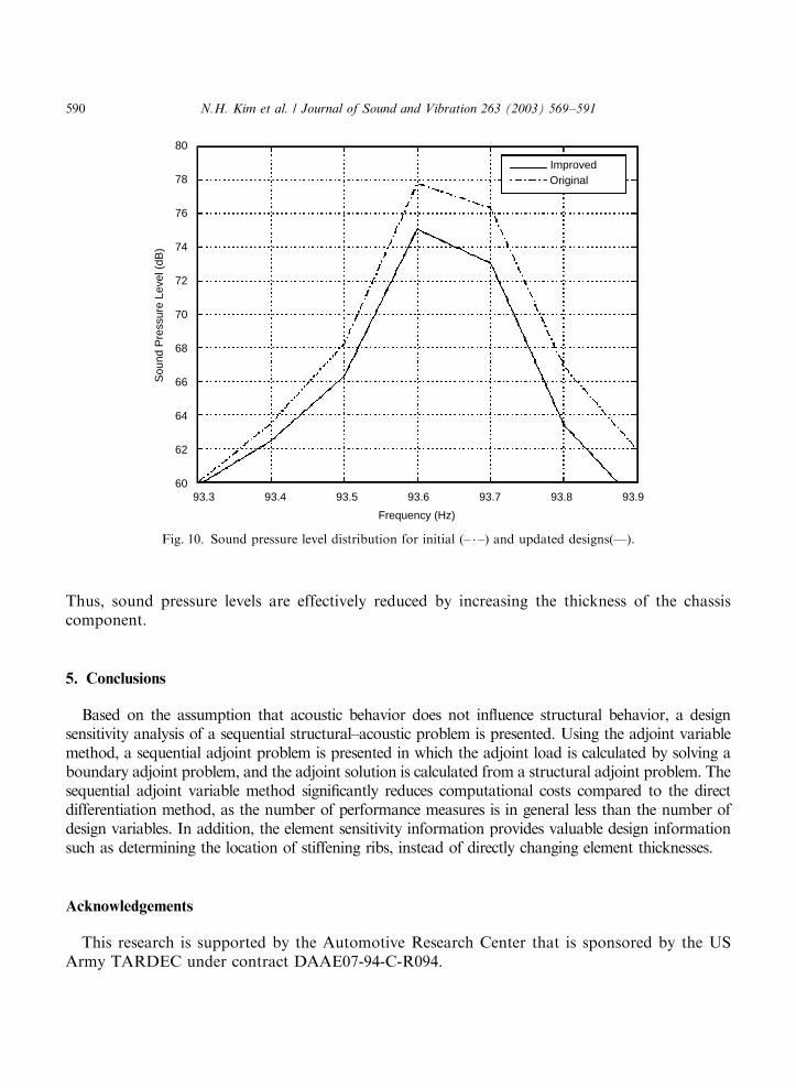
Thus, sound pressure levels are effectively reduced by increasing the thickness of the chassiscomponent.

5. Conclusions

Based on the assumption that acoustic behavior does not influence structural behavior, a designsensitivity analysis of a sequential structural–acoustic problem is presented. Using the adjoint variablemethod, a sequential adjoint problem is presented in which the adjoint load is calculated by solving aboundary adjoint problem, and the adjoint solution is calculated from a structural adjoint problem. Thesequential adjoint variable method significantly reduces computational costs compared to the directdifferentiation method, as the number of performance measures is in general less than the number ofdesign variables. In addition, the element sensitivity information provides valuable design informationsuch as determining the location of stiffening ribs, instead of directly changing element thicknesses.

Acknowledgements

This research is supported by the Automotive Research Center that is sponsored by the USArmy TARDEC under contract DAAE07-94-C-R094.

93.3 93.4 93.5 93.6 93.7 93.8 93.960

62

64

66

68

70

72

74

76

78

80S

ound

Pre

ssur

e Le

vel (

dB)

Frequency (Hz)

ImprovedOriginal

Fig. 10. Sound pressure level distribution for initial (– � –) and updated designs(—).


References

[1] Z.-D. Ma, I. Hagiwara, Sensitivity analysis-method for coupled acoustic–structural systems, Part 1: modal

sensitivities, American Institute of Aeronautics and Astronautics Journal 29 (1991) 1787–1795.

[2] Z.-D. Ma, I. Hagiwara, Sensitivity analysis-method for coupled acoustic–structural systems, Part 2: direct

frequency-response and its sensitivities, American Institute of Aeronautics and Astronautics Journal 29 (1991)

1796–1801.

[3] S. Wang, K.K. Choi, H. Kularni, Acoustical optimization of vehicle passenger space, SAE Paper No. 941071,

1994.

[4] K.K. Choi, I. Shim, S. Wang, Design sensitivity analysis of structure-induced noise and vibration, Journal of

Vibration and Acoustics 119 (1997) 173–179.

[5] D.J. Nefske, J.A. Wolf, L.J. Howell, Structural–acoustic finite element analysis of the automobile passenger

compartment: a review of current practice, Journal of Sound and Vibration 80 (1982) 247–266.

[6] R.R. Salagame, A.D. Belegundu, G.H. Koopman, Analytical sensitivity of acoustic power radiated from plates,

Journal of Vibration and Acoustics 117 (1995) 43–48.

[7] J.W. Rayleigh, The Theory of Sound, Dover Publications, New York, 1945.

[8] F. Scarpa, Parametric sensitivity analysis of coupled acoustic–structural systems, Journal of Vibration and

Acoustics 122 (2000) 109–115.

[9] D.C. Smith, R.J. Bernhard, Computation of acoustic shape design sensitivity using a boundary element method,

Journal of Vibration and Acoustics 114 (1992) 127–132.

[10] K.A. Cunefare, G.H. Koopman, Acoustic design sensitivity for structural radiators, Journal of Vibration and

Acoustics 114 (1992) 179–186.

[11] J.H. Kane, S. Mao, G.C. Everstine, Boundary element formulation for acoustic shape sensitivity analysis, Journal

of the Acoustical Society of America 90 (1991) 561–573.

[12] T. Matsumoto, M. Tanaka, Y. Yamada, Design sensitivity analysis of steady-state acoustic problems using

boundary integral equation formulation, JSME International Journal Series C 38 (1995) 9–16.

[13] B.U. Koo, Shape design sensitivity analysis of acoustic problems using a boundary element method, Computers &

Structures 65 (1997) 713–719.

[14] K.K. Choi, J.H. Lee, Sizing design sensitivity analysis of dynamic frequency response of vibrating structures,

American Society of Mechanical Engineers, Journal of Mechanical Design 114 (1992) 166–173.

[15] N. Vlahopoulos, S.T. Raveendra, C. Mollo, Acoustic sensitivity analysis using boundary elements and structural

dynamics response, Proceedings of the MSC User’s Conference, MacNeal-Schwendler Corp., Los Angeles, CA,

Paper 7, 1994.

[16] M.J. Allen, R. Sbzagio, N. Vlahopoulos, Structural/acoustic sensitivity analysis of a structure subject to stochastic

excitation, American Institute of Aeronautics and Astronautics Journal 39 (2001) 1270–1279.

[17] R.D. Ciskowski, C.A. Brebbia, Boundary Elements in Acoustics, Elsevier Applied Science, New York, 1991.

[18] E.J. Haug, K.K. Choi, V. Komkov, Design Sensitivity Analysis of Structural Systems, Academic Press, New York,

1985.

[19] J. Horvath, Topological Vector Spaces and Distributions, Addison-Wesley, London, 1966.

[20] A.D. Dimarogonas, Vibration Engineering, West Publishing Co., St. Paul, MN, 1976.

[21] P.K. Kythe, Introduction to Boundary Element Methods, CRS Press, Boca Raton, FL, 1995.

[22] J.N. Reddy, Applied Functional Analysis and Variational Methods in Engineering, McGraw-Hill, New York,

1986.

[23] T.J.R. Hughes, The Finite Element Method, Prentice-Hall, Englewood Cliffs, NJ, 1987.

[24] M.A. Gockel, MSC/NASTRAN Handbook for Dynamic Analysis, The MacNeal-Schwendler Corp., Los Angeles,

CA, 1983.


Design sensitivity analysis for sequential structural ... · Design sensitivity analysis for...

Documents

Transcript of Design sensitivity analysis for sequential structural ... · Design sensitivity analysis for...