Design, optimization, and characterization of multi-beam optical systems Maura Sandri

INAF IASF Bologna

1

Introduction

• The performance of an optical system can be quantified by two main quantities:

1. Image quality/efficiency:

• PSF/Strehl ratio (optical)

• Beam/efficiency (radio and mw)

2. Ability to point it in the right direction

• Image quality is determined by a proper design of the optical system, as well as accuracy and alignment of the manufactured optics.

2 Design and optimization of multi-beam optical systems

Overview of sub-efficiencies

3

(see Cappellen 2007)

Spillover and taper efficiencies

4

• The taper efficiency and the spillover efficiency are complementary:

as the taper increases, the spillover will decrease (and thus increases hsp), while the taper efficiency ht decreases.

• The trade-off between hsp and ht has an optimum solution: -11 dB.

ET(dB) = 10 Log10 𝑃𝑒𝑑𝑔𝑒

𝑃𝑐𝑒𝑛𝑡𝑟𝑒

Uniform illumination Tapered illumination

Some examples of ET (radio)

ALMA -12 dB

GBT -14 dB

VLA -12 dB

SRT -12 dB

5

Planck -30 dB

WMAP -20 dB

Some examples of ET (cmb)

6

Trade-off angular resolution and straylight

The taper used in the CMB experiments are rather different because we have strong requirements in the straylight rejection due to the fact that straylight contamination, originated by the signal entering the feed horns through the sidelobes of the radiation patter, could be higher than the CMB signal when the sidelobes points towards the Galactic plane.

• Far-field pattern is the Fourier transform of aperture plane electric field distribution:

• Uniform illumination sinc function

• Gaussian illumination Gaussian function

• Software packages for precise modelling of reflector antennas and beam simulations (GRASP)

Single beam optics

7

Psky = Optics(Pfeed)

Multi-beams optics

𝑟 𝑠𝑘𝑦 = 𝑂𝑝𝑡𝑖𝑐𝑠 𝑥𝑓𝑒𝑒𝑑 , 𝑦𝑓𝑒𝑒𝑑

𝑧𝑓𝑒𝑒𝑑 = 𝑧 𝑥𝑓𝑒𝑒𝑑 , 𝑦𝑓𝑒𝑒𝑑

• Illumination (ET) • Beam pointing

• Feed locations • Tilting

• Feed mechanical coupling • Feed e.m. coupling • Constrains in array dimensions

𝑃𝑠𝑘𝑦 = 𝑂𝑝𝑡𝑖𝑐𝑠 𝑃𝑓𝑒𝑒𝑑

8

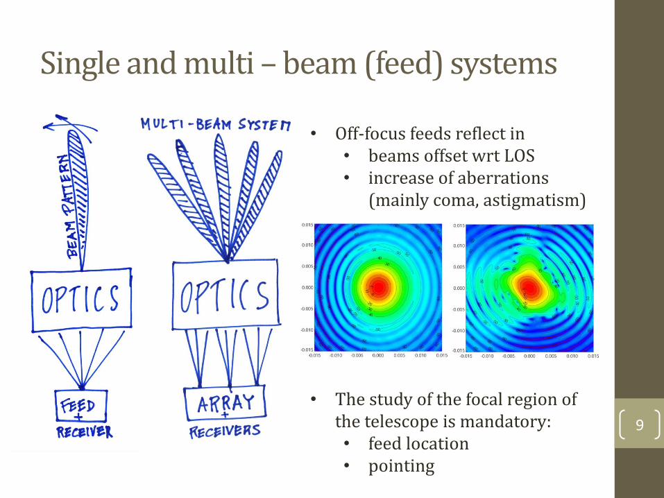
Single and multi – beam (feed) systems

9

• Off-focus feeds reflect in • beams offset wrt LOS • increase of aberrations

(mainly coma, astigmatism)

• The study of the focal region of the telescope is mandatory: • feed location • pointing

Focal plane surface arrays

10

Concave focal surface Convex focal surface Single feed at focus: feed boresight along telescope chief-ray

A strategy to locate and tilt the feeds is required

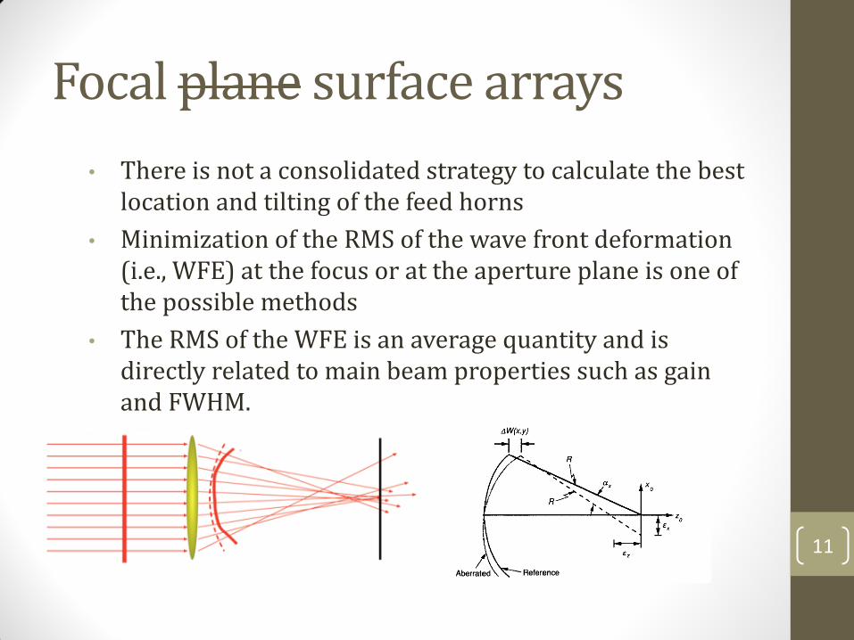
Focal plane surface arrays

• There is not a consolidated strategy to calculate the best location and tilting of the feed horns

• Minimization of the RMS of the wave front deformation (i.e., WFE) at the focus or at the aperture plane is one of the possible methods

• The RMS of the WFE is an average quantity and is directly related to main beam properties such as gain and FWHM.

11

Shape of the focal surface

12

What does optimisation mean?

• Minimise the main beam distortions

• Minimise the straylight contamination

• Improve the angular resolution

• Make the focal surface as flat as possible

• Fit the telescope/focal plane into the fairing (space)

13

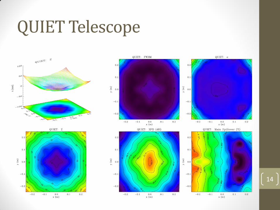
QUIET Telescope

14

Planck Telescope

15

Summarizing …

• Multi beam systems are widely used to improve image capabilities for millimeter and radio-telescopes (sky coverage and sensitivity)

• The complication is that feed dimensions are not negligible so that off-axis aberrations may degrade the beam patterns rapidly

• Location and pointing of feeds need to be carefully studied to minimize illumination losses and spillover radiation

• Complicated system w.r.t single feed optics especially in polarization since the polarization capabilities degrades far from optical axis.

16

Planck: a case study. Why?

• Planck is a multi-beam, multi-frequency telescope

• High performance, low systematics focal plane instrumentation spanning in frequency from 27GHz to 1THz with 74 detectors and 47 corrugated feed horns

• Almost 10 years of telescope and focal plane optimization activity to satisfy the demanding performances required by precision CMB measurements

• It has been characterized very well (on-ground and in-flight) to remove the systematic effects

17

The Planck Optics

18

REFERENCES Sandri et al., Low Frequency Instrument Optics, A&A 520, A7 (2010) Tauber et al., The Optical System, A&A 520, A2 (2010)

Telescope design and optimization

• (1996) We started with a Dragone-Mizuguchi 1.3 meter aperture Telescope (Gregorian off-axis configuration)

• (1998) We moved towards a quasi Dragone-Mizuguchi 1.5 meter aperture Telescope

• (1999) We demonstrated that Aplanatic (optical) condition may optimize the main beam shape

• (2000) We optimized the optics using traditional ‘optical’ software at various Planck frequencies (APLANATISATION).

• (2000-2002) We designed the focal plane and the corrugated feed horns to satisfy the angular resolution and the straylight requirements

• (2004) focal plane unit design frozen after re-optimization (including polarisation)

19

Focal plane, feed pattern and illumination

20

10 dB contours

Trade-off between AR and spillover

21

Taper

[dB @ °]

e

FWHM

[arcmin]

Directivity

[dBi]

30 @ 22 1.20 13,08 58.8

23 @ 22 1.16 12,06 59.4

15 @ 22 1.15 11,10 59.9

10 @ 22 1.18 10,74 59.7

ET 30 dB @ 22° ET 23 dB @ 22°

ET 15 dB @ 22° ET 10 dB @ 22°

10 dB of ET degradation ~ factor of 10 in the Galactic straylight

Where sidelobes come from?

22

Main Spillover

(a)

Main Spillover

(b)

Sub Spillover (b)

Sub Spillover

(a)

MB

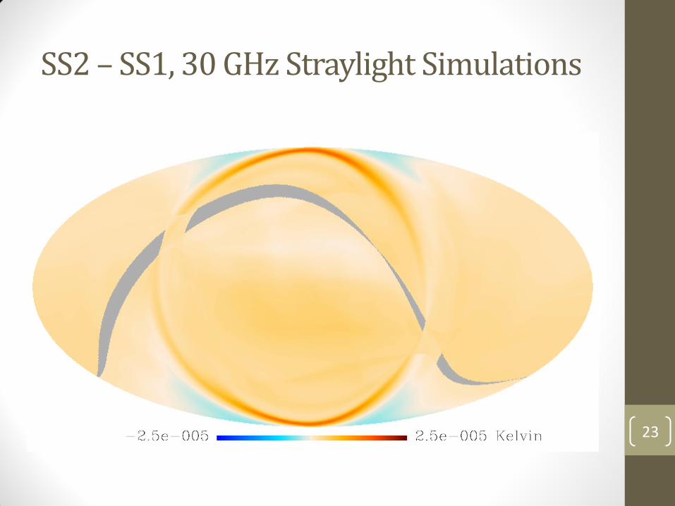
SS2 – SS1, 30 GHz Straylight Simulations

23

SS2 – SS1, 30 GHz dDX9

24

SS2 – SS1, 30 GHz dDX9 - Sim

25

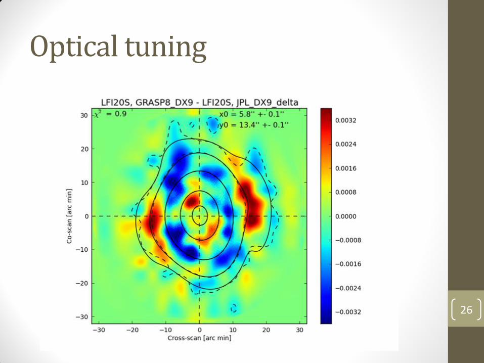
Optical tuning

26

Lesson learned from Planck

• Requirements should be properly defined taking into account

• bandpass response

• asymmetric illumination typical of multi-beam systems (the edge taper is not a number but it is a curve)

• Beam simulations are a fundamental tool from design phase to sky measurements

• to guarantee correct gain values in the calibration pipeline

• to remove systematics from the maps

• Polarization purity degrades in multi-beam optics

• cross-polarization is quite impossible to be properly characterized with celestial sources

• beam simulations are mandatory to model the beam polarization

• Good optical simulations require excellent measurements of the optical components (feed, reflector surfaces, alignment)

27