Design of spatial microphone arrays for sound field ...

HAL Id: hal-01148971https://hal.inria.fr/hal-01148971

Submitted on 6 May 2015

HAL is a multi-disciplinary open accessarchive for the deposit and dissemination of sci-entific research documents, whether they are pub-lished or not. The documents may come fromteaching and research institutions in France orabroad, or from public or private research centers.

L’archive ouverte pluridisciplinaire HAL, estdestinée au dépôt et à la diffusion de documentsscientifiques de niveau recherche, publiés ou non,émanant des établissements d’enseignement et derecherche français ou étrangers, des laboratoirespublics ou privés.

Design of spatial microphone arrays for sound fieldinterpolation

Gilles Chardon, Wolfgang Kreuzer, Markus Noisternig

To cite this version:Gilles Chardon, Wolfgang Kreuzer, Markus Noisternig. Design of spatial microphone arrays forsound field interpolation. IEEE Journal of Selected Topics in Signal Processing, IEEE, 2015, pp.11.10.1109/JSTSP.2015.2412097. hal-01148971

https://hal.inria.fr/hal-01148971

https://hal.archives-ouvertes.fr

1

Design of spatial microphone arrays for sound fieldinterpolation

Gilles Chardon, Member, IEEE, Wolfgang Kreuzer, and Markus Noisternig, Member, IEEE

Abstract—This article presents a design method for micro-phone arrays with arbitrary geometries. Based on a theoreticalanalysis and on the magic points method, it allows for theinterpolation of a sound field in a generic convex domain witha limited number of microphones on a given frequency band. Itis shown that only a few microphones are needed in the interiorof the considered domain to ensure a low interpolation error inthe frequency band of interest, and that most of the microphoneshave to be located on the boundary of the domain, with a non-uniform density depending on the shape of the domain. Practicaldesign constraints can be included in the optimization process.Comparisons for some particular array geometries with designmethods known from the literature are given, showing that theproposed approach results in lower errors.

Index Terms—sound field analysis, array processing, micro-phone arrays, numerical robustness

I. INTRODUCTION

THIS paper deals with the spatial interpolation of soundfields by microphone arrays of general shapes. Although

the interpolation error is seldom-used as a performance mea-sure for microphone arrays, its use can be justified by thefollowing two main arguments. Firstly, theoretical results oninterpolation and sampling of functions are widely available,and are the subject of ongoing research (see e.g. compressedsensing). Secondly, a microphone array that is able to interpo-late the sound field in some spatial domain should be able tosimulate the measurements of any other microphone array inthe same domain. It thus should perform similarly in terms ofdifferent array performance measures, such as the white noisegain, the condition number, and the estimation of the sphericalharmonics expansion coefficients.

Spherical microphone arrays are upon the most widelyused array geometries for 3-D sound field recording. Earlystudies on open spherical microphone arrays have shown thatnumerical instabilities appear at some wave numbers, which

Copyright (c) 2014 IEEE. Personal use of this material is permitted.However, permission to use this material for any other purposes must beobtained from the IEEE by sending a request to [email protected]

G. Chardon was with the Acoustics Research Institute, Austrian Academyof Sciences, Vienna, during part of the preparation of this article, andis now with the Laboratoire des Signaux et Systemes (L2S), Centrale-Supelec, CNRS UMR 8506, Univ. Paris Sud, Gif-sur-Yvette, France (e-mail:[email protected]).

W. Kreuzer is with the Acoustics Research Institute, Austrian Academy ofSciences, Vienna, Austria (e-mail: [email protected]).

M. Noisternig is with the Acoustic and Cognitive Spaces Research Groupat IRCAM, CNRS, Sorbonne Universites, UPMC Universite Paris 6, UMR9912 STMS, Paris, France (e-mail: [email protected]).

Parts of the preliminary work related to the current manuscript appeared inthe Proceedings of the IEEE International Conference on Acoustics, Speech,and Signal Processing (ICASSP 2014).

are related to the roots of the spherical Bessel functions (cf.[1], [2]). Meyer and Elko [3] proposed to overcome thisproblem by placing the microphones on a rigid, sound hardsphere. This approach is not very well suited for arrays withlarge radii and several authors have proposed alternative arraygeometries. One way to increase the stability around the rootsof the Bessel functions, without the drawback of introducinga rigid sphere into the measured sound field, is to use cardioidmicrophones facing outwards in radial direction (cf. [4], [5],[6]). In practice, this approach is difficult to realize, sincecardioid microphones have a relatively high noise level atlow frequencies. This solution is also prone to microphonepositioning and steering errors, as well as to imperfectionsin the microphone directivity patterns. Double-sphere arraysprovide an alternative solution to the ill-conditioning problemof open-sphere arrays (cf. [6], [7], [8]). They typically consistof pressure microphones arranged on two concentric spheres(i.e. two open spheres or, alternatively, an inner rigid sphereplus an outer open sphere) with different radii. This approachis particularly well suited for arrays with a large aperture thatalso covers the lower frequency range. The main drawbackof a double-sphere array is that it requires at least twice thenumber of microphones of a single-sphere array.

Some authors proposed the use of non-spherical arraygeometries for increasing the stability around the roots of theBessel functions. Rafaely [9] showed that an open sphericalshell array (i.e. where some microphones are moved from theboundary to the inside of the sphere) can achieve robustness ona large frequency band. The positions of the interior samplingpoints are determined by a constrained nonlinear optimizationprocedure that minimizes the maximal condition number ofthe matrix that contains the product of the spherical Besselfunctions with the spherical harmonics. With this method itis, however, not straightforward to determine the number ofinterior sampling points that, for a given array order, ensurestability and convergence of the optimization routine. Abhaya-pala and Gupta [10] proposed a hybrid array geometry thatuses pairs of circular arrays to sample the three-dimensionalsound field. This approach puts lesser restrictions on sensorlocations and allows for an increased operating bandwidth.Another attempt to overcome the problem of zero-valuedBessel functions is the double-sided cone array [11]. It exploitsthe radial orthogonality of the spherical Bessel functions,evaluated on the surface of a double-sided cone, to estimatethe spherical harmonics expansion coefficients over a relativelywide frequency range. Anyway, it has been shown that theestimation fails for some frequencies. This can only be avoidedby sampling the sound field at two or more cones and therefore

This is the author's version of an article that has been published in this journal. Changes were made to this version by the publisher prior to publication.The final version of record is available at http://dx.doi.org/10.1109/JSTSP.2015.2412097

Copyright (c) 2015 IEEE. Personal use is permitted. For any other purposes, permission must be obtained from the IEEE by emailing [email protected].

2

requires a relatively large number of microphones. The spindletorus array [12] is obtained by projecting a uniform sampledistribution on the sphere to a self-intersecting torus. Thisarray achieves robustness against noise and can be easilyimplemented by a scanning microphone setup. However, theincreased robustness comes for the expense of a relatively highnumber of required sampling nodes.

Mignot et al. [13] introduced an interpolation method forroom impulse responses at low frequencies. This methodapproximates the sound field by sums of plane waves usingmeasurements of the sound field on an array of randomlyplaced microphones. The design of the sampling grid was,however, not analyzed and is very likely suboptimal. In [14],it has been shown that for time-limited signals (such as roomimpulse responses) nonuniform sampling in the frequencydomain can be used to avoid samples near the Bessel nulls. Theoptimal positions of the samples in the frequency domain canbe numerically obtained by minimizing the condition numberof the Fourier matrix and the diagonal matrix holding valuesof the spherical Bessel function.

In [15], Chardon et al. presented an optimal design (with re-spect to the number of sampling points) for open spherical mi-crophone arrays by adding few microphones inside the sphere.The number and the positioning of these microphones aredependent on the eigenmodes of the sphere in the wavenumberdomain of interest. The work presented in this paper is ageneralization of the design method presented in [15] togeneral domains (for example ellipsoidal or cubical arrays).We discuss stability issues for sound field interpolation, andpresent some examples of more general measurement arrays,including a discussion on how to impose constraints on thedesign in order to deal with practical issues for buildingmicrophone arrays.

The paper is organized as follows: Section II gives abrief introduction into the approximation of wave fields anddescribes the microphone array performance measure appliedin this study. In Section III, we first discuss the stability ofsound field interpolation with spherical and non-spherical mi-crophone arrays and then how the choice of a basis influencesthe stability of sound field representation. Several possibilitiesfor designing microphone arrays are introduced in Section IV.In this section we discuss both the sampling on the domain’ssurface and how some interior points stabilize the arrayaround unstable frequencies (e.g., Bessel nulls in the particularcase of a spherical array). In Section V, the performance ofspherical and ellipsoidal microphone arrays is compared usingnumerical simulations. The results highlight the effectivenessand flexibility of our method. However, when applying the pro-posed optimization method to spherical microphone arrays theinterior sampling points are spread over the entire inner vol-ume, which in practice may lead to problems with constructingthe array. In Section VI, we therefore introduce a modifiedoptimization method for determining the interior samplingpositions that allows to include sampling constraints. Applyingthis method to three example arrays (a double sphere, a mixedsphere, and a spindle torus array; all with additional interiorsampling points) shows how practical constraints are includedinto optimized spatial sampling, and how this improves the

robustness and simplifies the practical implementation of thesearrays. Concluding remarks are given in Section VII. Thecode to reproduce the results of this paper is available athttp://gilleschardon.fr/jstsp_array.

II. PRELIMINARIES

A. Performance measures

Microphone arrays can be used for a wide variety oftasks, e.g., sound source localization, beamforming, and soundfield analysis. Various metrics can be applied to measurethe performance of a microphone array, such as the whitenoise gain, the directivity index, and the condition numberof the estimation of the spherical harmonics series expansioncoefficients (see e.g. [16] for further quality metrics). In aprevious study [15], we compared the performance of differentopen spherical arrays with respect to the interpolation error,the condition number, and the white noise gain.

In this work, we will use the interpolation error of the soundfield inside the volume of the array as the main performancemeasure. This error is defined as the L2 norm of the differencebetween the actual sound field p and its interpolation pobtained from a finite number of measurements:

‖p− p‖ =

∫Ω

|p− p|2 (1)

For numerical integration adequate quadrature rules are ap-plied. In this article, the sound pressure p is approximatedin the domain of interest Ω by spherical harmonics approx-imations (cf. equation (3)); the spherical harmonics expan-sion coefficients were determined by least-squares estimation.While interpolation of the sound field is not always the goalof microphone array processing, the justification of the use ofthis measure for the design of microphone arrays is threefold:(i) the interpolation error is easy to estimate, (ii) theoreticalresults are available and can be used to guide the design of anarray, and, what is even more important, (iii) the interpolationerror can be used to represent any other performance measure.A microphone array, which is able to interpolate the soundfield in its volume with a low number of microphones anda small interpolation error, is able to simulate any othermicrophone array included in the same volume, and thusinherits its performance.

B. Approximation of acoustical fields

Moiola et al. [17] rigorously studied the approximation ofacoustical fields in the harmonic regime (or, more generally, ofsolutions to the Helmholtz equation). The main result of thesestudies is that a general solution u to the Helmholtz equation

∆u+ k2u = 0 (2)

in a star-convex domain Ω (i.e. there exists a point O suchthat any point in the domain Ω can be linked to O by asegment included in the domain) can be approximated by alinear combination of spherical harmonics

u ≈L∑l=0

l∑m=−l

αLlmjl(kr)Ylm(θ, φ) (3)



3

in spherical coordinates (r, θ, φ), where jl is the l-th sphericalBessel function and Ylm are the spherical harmonics. Alterna-tively, the solutions can be as well approximated by a linearcombination of plane waves

u ≈J∑j=1

βJj exp(i~kj · ~x), (4)

where the wavevectors ~kj are sampled on the sphere of radiusk in the wavenumber space. The convergence rate of thoseapproximations depends on the smoothness of u. In mostapplications, u is smooth and the convergence is exponential[18].

In the harmonic regime, the pressure field is a solution to theHelmholtz equation (2). It is thus possible to use the aboveintroduced schemes to approximate sound fields in generalconvex domains.

Note that the expansion coefficients αLlm and βJj depend onthe order of approximation L and J , respectively. A sphericalharmonics series expansion of the acoustical field does notnecessarily exist for general domains. A sphere centered atthe origin is the only domain for which it is guaranteed thatall acoustical fields can be represented as a series of sphericalharmonics. For other domains, the sound field can only beapproximated by finite sums of spherical harmonics, with anapproximation error that tends to zero as the approximationorder tends to infinity. This, however, has no consequences forthe task at hand, and spherical harmonics can be safely usedto interpolate the sound field in general star-convex domains.

III. STABILITY OF SOUND FIELD INTERPOLATION

In this section, we study the interpolation of a sound fieldp from a finite number of punctual samples (i.e. pressuremicrophones) in a volume Ω. The interpolation is obtainedby least-squares estimation of the coefficients of a finite-dimensional approximation p of the sound field, using planewaves, spherical harmonics, or other families of functions.

Stability is guaranteed when the interpolation error ‖p− p‖is of the same order as the best approximation error ‖p− p‖,where p is the best approximation of p in the chosen finitedimensional space. In general, having more measurements thandegrees of freedom is not sufficient to ensure the stability ofthe interpolation (cf. Runge phenomenon [19]).

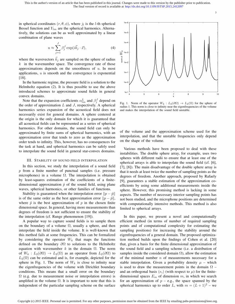
A popular way to capture sound fields is to sample themon the boundary of a volume Ω, usually a sphere, and theninterpolate the field inside the volume. It is well-known thatthis method fails at some frequencies. This can be formalizedby considering the operator Wk that maps the functionsdefined on the boundary ∂Ω to solutions to the Helmholtzequation with wavenumber k in the domain Ω. The normof Wk : L2(∂Ω) → L2(Ω) as an operator from L2(∂Ω) toL2(Ω) can be estimated and is, for example, depicted for thesphere in Fig. 1. The norm of Wk is close to infinity nearthe eigenfrequencies of the volume with Dirichlet boundaryconditions. This means that a small error on the boundaryΩ (e.g. due to measurement noise or interpolation errors) isamplified in the volume Ω. It is important to note that this isindependent of the particular sampling scheme on the surface

4 5 6 7 8 9 10

1e-1

1e+0

1e+1

1e+2

1e+3

1e+4

1e+5

1e+6

k

no

rm o

f

Fig. 1. Norm of the operator Wk : L2(∂Ω) → L2(Ω) for the sphere ofradius 1. This norm is close to infinity near the eigenfrequencies of the volumeand makes the interpolation of the sound field unstable.

of the volume and the approximation scheme used for theinterpolation, and that the unstable frequencies only dependon the shape of the volume.

Various methods have been proposed to deal with theseinstabilities. The double sphere array, for example, uses twospheres with different radii to ensure that at least one of thespherical arrays is able to interpolate the sound field (cf. [6],[7], [8]). The main disadvantage of the double sphere array isthat it needs at least twice the number of sampling points as thedegrees of freedom. Another approach, proposed by Rafaely[9], guarantees a stable estimation of the approximation co-efficients by using some additional measurements inside thesphere. However, this promising method is lacking in someaspects. The number of necessary interior sampling points hasnot been studied, and the microphone positions are determinedwith computationally intensive methods. This method is alsolimited to spherical arrays.

In this paper, we present a novel and computationallyefficient method (in terms of number of required samplingpoints and of computational complexity for estimating thesampling positions) for increasing the stability around theeigenfrequencies of a general domain. The proposed optimiza-tion method builds upon the findings of Cohen et al. [20]that, given a basis for the finite dimensional approximation ofthe sound field and a sampling scheme (i.e. a distribution ofsamples inside the considered domain Ω), allow the estimationof the minimal number n of measurements necessary for astable interpolation. Given a probability density µ – whichis used to draw the measurement points in the domain Ω –and an orthogonal basis (ei) (with respect to µ) for the finite-dimensional spaces Em of dimension m, in which we searchfor an approximation of p – e.g., the space spanned by thespherical harmonics up to order L, with m = (L+ 1)2 – we



4

can compute the quantity

K(m) = maxx∈Ω

m∑j=1

|ej(x)|2. (5)

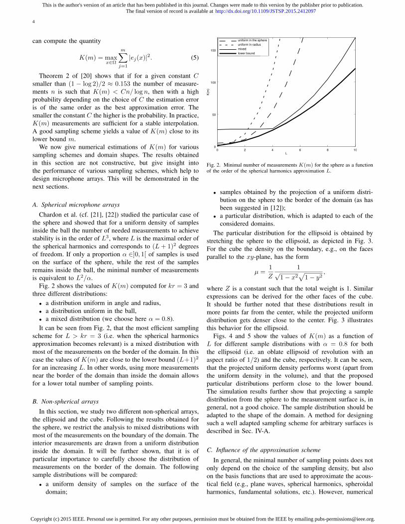
Theorem 2 of [20] shows that if for a given constant Csmaller than (1 − log 2)/2 ≈ 0.153 the number of measure-ments n is such that K(m) < Cn/ log n, then with a highprobability depending on the choice of C the estimation erroris of the same order as the best approximation error. Thesmaller the constant C the higher is the probability. In practice,K(m) measurements are sufficient for a stable interpolation.A good sampling scheme yields a value of K(m) close to itslower bound m.

We now give numerical estimations of K(m) for varioussampling schemes and domain shapes. The results obtainedin this section are not constructive, but give insight intothe performance of various sampling schemes, which help todesign microphone arrays. This will be demonstrated in thenext sections.

A. Spherical microphone arrays

Chardon et al. (cf. [21], [22]) studied the particular case ofthe sphere and showed that for a uniform density of samplesinside the ball the number of needed measurements to achievestability is in the order of L3, where L is the maximal order ofthe spherical harmonics and corresponds to (L+ 1)2 degreesof freedom. If only a proportion α ∈]0, 1[ of samples is usedon the surface of the sphere, while the rest of the samplesremains inside the ball, the minimal number of measurementsis equivalent to L2/α.

Fig. 2 shows the values of K(m) computed for kr = 3 andthree different distributions:• a distribution uniform in angle and radius,• a distribution uniform in the ball,• a mixed distribution (we choose here α = 0.8).It can be seen from Fig. 2, that the most efficient sampling

scheme for L > kr = 3 (i.e. when the spherical harmonicsapproximation becomes relevant) is a mixed distribution withmost of the measurements on the border of the domain. In thiscase the values of K(m) are close to the lower bound (L+1)2

for an increasing L. In other words, using more measurementsnear the border of the domain than inside the domain allowsfor a lower total number of sampling points.

B. Non-spherical arrays

In this section, we study two different non-spherical arrays,the ellipsoid and the cube. Following the results obtained forthe sphere, we restrict the analysis to mixed distributions withmost of the measurements on the boundary of the domain. Theinterior measurements are drawn from a uniform distributioninside the domain. It will be further shown, that it is ofparticular importance to carefully choose the distribution ofmeasurements on the border of the domain. The followingsample distributions will be compared:• a uniform density of samples on the surface of the

domain;

0 2 4 6 8 100

50

100

150

L

K(m

)

uniform in the sphere

uniform in radius

mixed

lower bound

Fig. 2. Minimal number of measurements K(m) for the sphere as a functionof the order of the spherical harmonics approximation L.

• samples obtained by the projection of a uniform distri-bution on the sphere to the border of the domain (as hasbeen suggested in [12]);

• a particular distribution, which is adapted to each of theconsidered domains.

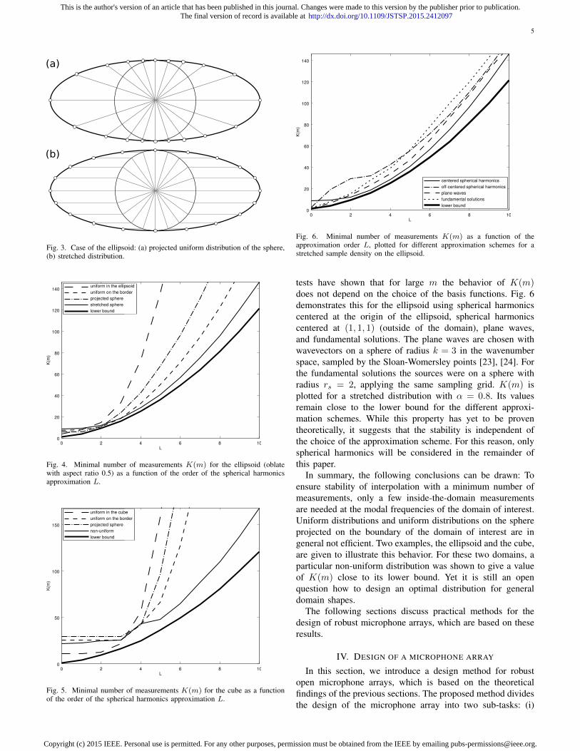
The particular distribution for the ellipsoid is obtained bystretching the sphere to the ellipsoid, as depicted in Fig. 3.For the cube the density on the boundary, e.g., on the facesparallel to the xy-plane, has the form

µ =1

Z

1√

1− x2√

1− y2,

where Z is a constant such that the total weight is 1. Similarexpressions can be derived for the other faces of the cube.It should be further noted that these distributions result inmore points far from the center, while the projected uniformdistribution gets denser close to the center. Fig. 3 illustratesthis behavior for the ellipsoid.

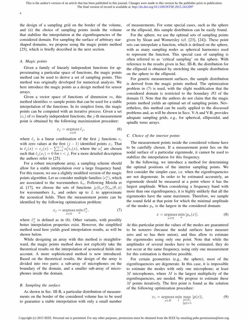
Figs. 4 and 5 show the values of K(m) as a function ofL for different sample distributions with α = 0.8 for boththe ellipsoid (i.e. an oblate ellipsoid of revolution with anaspect ratio of 1/2) and the cube, respectively. It can be seen,that the projected uniform density performs worst (apart fromthe uniform density in the volume), and that the proposedparticular distributions perform close to the lower bound.The simulation results further show that projecting a sampledistribution from the sphere to the measurement surface is, ingeneral, not a good choice. The sample distribution should beadapted to the shape of the domain. A method for designingsuch a well adapted sampling scheme for arbitrary surfaces isdescribed in Sec. IV-A.

C. Influence of the approximation scheme

In general, the minimal number of sampling points does notonly depend on the choice of the sampling density, but alsoon the basis functions that are used to approximate the acous-tical field (e.g., plane waves, spherical harmonics, spheroidalharmonics, fundamental solutions, etc.). However, numerical



5

(a)

(b)

Fig. 3. Case of the ellipsoid: (a) projected uniform distribution of the sphere,(b) stretched distribution.

0 2 4 6 8 100

20

40

60

80

100

120

140

L

K(m

)

uniform in the ellipsoid

uniform on the border

projected sphere

stretched sphere

lower bound

Fig. 4. Minimal number of measurements K(m) for the ellipsoid (oblatewith aspect ratio 0.5) as a function of the order of the spherical harmonicsapproximation L.

0 2 4 6 8 100

50

100

150

L

K(m

)

uniform in the cube

uniform on the border

projected sphere

non-uniform

lower bound

Fig. 5. Minimal number of measurements K(m) for the cube as a functionof the order of the spherical harmonics approximation L.

0 2 4 6 8 100

20

40

60

80

100

120

140

L

K(m

)

centered spherical harmonics

off-centered spherical harmonics

plane waves

fundamental solutions

lower bound

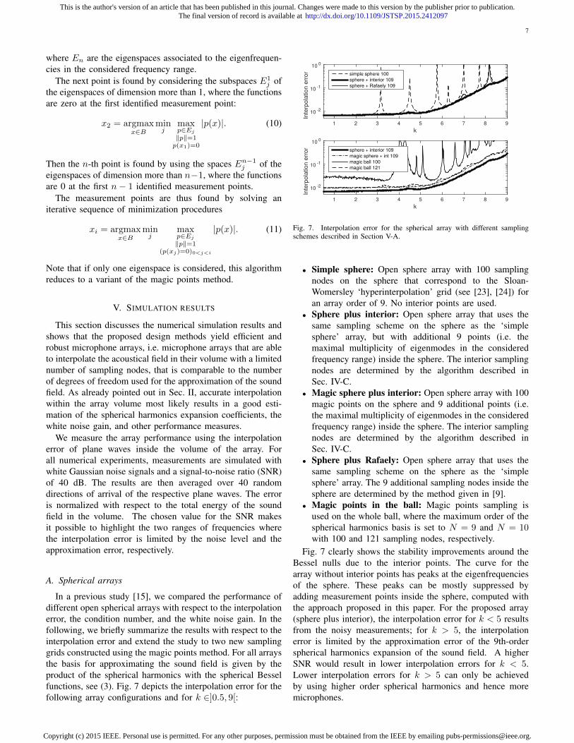
Fig. 6. Minimal number of measurements K(m) as a function of theapproximation order L, plotted for different approximation schemes for astretched sample density on the ellipsoid.

tests have shown that for large m the behavior of K(m)does not depend on the choice of the basis functions. Fig. 6demonstrates this for the ellipsoid using spherical harmonicscentered at the origin of the ellipsoid, spherical harmonicscentered at (1, 1, 1) (outside of the domain), plane waves,and fundamental solutions. The plane waves are chosen withwavevectors on a sphere of radius k = 3 in the wavenumberspace, sampled by the Sloan-Womersley points [23], [24]. Forthe fundamental solutions the sources were on a sphere withradius rs = 2, applying the same sampling grid. K(m) isplotted for a stretched distribution with α = 0.8. Its valuesremain close to the lower bound for the different approxi-mation schemes. While this property has yet to be proventheoretically, it suggests that the stability is independent ofthe choice of the approximation scheme. For this reason, onlyspherical harmonics will be considered in the remainder ofthis paper.

In summary, the following conclusions can be drawn: Toensure stability of interpolation with a minimum number ofmeasurements, only a few inside-the-domain measurementsare needed at the modal frequencies of the domain of interest.Uniform distributions and uniform distributions on the sphereprojected on the boundary of the domain of interest are ingeneral not efficient. Two examples, the ellipsoid and the cube,are given to illustrate this behavior. For these two domains, aparticular non-uniform distribution was shown to give a valueof K(m) close to its lower bound. Yet it is still an openquestion how to design an optimal distribution for generaldomain shapes.

The following sections discuss practical methods for thedesign of robust microphone arrays, which are based on theseresults.

IV. DESIGN OF A MICROPHONE ARRAY

In this section, we introduce a design method for robustopen microphone arrays, which is based on the theoreticalfindings of the previous sections. The proposed method dividesthe design of the microphone array into two sub-tasks: (i)



6

the design of a sampling grid on the border of the volume,and (ii) the choice of sampling points inside the volumethat stabilize the interpolation at the eigenfrequencies of theconsidered domain. For sampling the surface of arbitrary star-shaped domains, we propose using the magic points method[25], which is briefly described in the next section.

A. Magic points

Given a family of linearly independent functions for ap-proximating a particular space of functions, the magic pointsmethod can be used to derive a set of sampling points. Thismethod was originally developed for numerical analysis. Wehere introduce the magic points as a design method for sensorarrays.

Given a vector space of functions of dimension m, thismethod identifies m sample points that can be used for a stableinterpolation of the functions. In its simplest form, the magicpoints can be computed with an iterative process. Given a set(ei) of m linearly independent functions, the j-th measurementpoint is obtained by the following maximization procedure:

xj = argmaxx∈Ω

ej , (6)

where ej is a linear combination of the first j functions eiwith zero values at the first (j − 1) identified points xi. Thatis ej(x) = ej(x) −

∑j−1i=1 α

ji ei(x), where the αji are chosen

such that ej(xi) = 0 for i < j. For a more detailed descriptionthe authors refer to [25].

For a robust microphone array, a sampling scheme shouldallow for a stable interpolation over a large frequency band.For this reason, we use a slightly modified version of the magicpoints algorithm. Let us consider multiple families (eni ), whichare associated to the wavenumbers kn. Following Moiola etal. [17], we choose the sets of functions jl(knr)Ylm(θ, φ)for wavenumbers kn and orders up to L to approximatethe acoustical fields. Then the measurement points can beidentified by the following optimization problem:

xj = argmaxx∈Ω

minnenj , (7)

where enj is defined as in (6). Other variants, with possiblybetter interpolation properties exist. However, the simplifiedmethod used here yields good interpolation results, as will beshown below.

While designing an array with this method is straightfor-ward, the magic points method does not explicitly take thetheoretical results on the interpolation of acoustical fields intoaccount. A more sophisticated method is now introduced.Based on the theoretical results, the design of the array isdivided into two parts: a sub-array of microphones on theboundary of the domain, and a smaller sub-array of micro-phones inside the domain.

B. Sampling the surface

As shown in Sec. III-B, a particular distribution of measure-ments on the border of the considered volume has to be usedto guarantee a stable interpolation with only a small number

of measurements. For some special cases, such as the sphereor the ellipsoid, this sample distribution can be easily found.

For the sphere, we use the optimal sets of sampling pointsgiven by Sloan and Womersley (cf. [23], [24]). These pointsets can interpolate a function, which is defined on the sphere,with as many sampling nodes as spherical harmonics usedto represent the function. This special case of sampling isoften referred to as ‘critical sampling’ on the sphere. Withreference to the results given in Sec. III-B, the distribution forthe ellipsoid is obtained by stretching the sample distributionon the sphere to the ellipsoid.

For generic measurement surfaces, the sample distributionis derived from the magic points method. The optimizationproblem in (7) is used, with the slight modification that theconsidered domain is restricted to the boundary ∂Ω of thedomain Ω. Note that the authors do not claim that the magicpoints method yields an optimal set of sampling points. Nev-ertheless, this method can be easily applied to the discussedproblems and, as will be shown in Secs. V-A and V-B, providesadequate sampling grids, e.g., for spherical, ellipsoidal, andspindle torus arrays.

C. Choice of the interior points

The measurement points inside the considered volume haveto be carefully chosen. If a measurement point lies on thenodal surface of a particular eigenmode, it cannot be used tostabilize the interpolation for this frequency.

In the following, we introduce a method for determiningthe optimal positions of the interior sampling points. Wefirst consider the simpler case, i.e. when the eigenfrequenciesare not degenerate. In order to be estimated accurately, aneigenmode should be measured at a point where it has thelargest amplitude. When considering a frequency band withmore than one eigenfrequency, it is highly unlikely that all theeigenmodes have the same maximum. Therefore, we samplethe sound field at that point for which the minimal amplitudeof the modes pn is the largest in the considered domain:

x = argmaxx∈Ω

minn|pn(x)|. (8)

At this particular point the values of the modes are guaranteedto be nonzero (because the nodal surfaces have measurezero and so has their union), and thus allow to estimatethe eigenmodes using only one point. Note that while theamplitudes of several modes have to be estimated, they donot occur at the same frequency, using only one measurementfor this estimation is therefore possible.

For certain geometries (e.g., the sphere), most of theeigenfrequencies are degenerate. In this case, it is impossibleto estimate the modes with only one microphone; at leastM microphones, where M is the largest multiplicity of theeigenfrequencies, are needed. We propose to estimate theseM points iteratively. The first point is found as the solutionof the following optimization procedure:

x1 = argmaxx∈B

minj

maxp∈Ej

‖p‖=1

|p(x)|, (9)



7

where En are the eigenspaces associated to the eigenfrequen-cies in the considered frequency range.

The next point is found by considering the subspaces E1j of

the eigenspaces of dimension more than 1, where the functionsare zero at the first identified measurement point:

x2 = argmaxx∈B

minj

maxp∈Ej

‖p‖=1p(x1)=0

|p(x)|. (10)

Then the n-th point is found by using the spaces En−1j of the

eigenspaces of dimension more than n−1, where the functionsare 0 at the first n− 1 identified measurement points.

The measurement points are thus found by solving aniterative sequence of minimization procedures

xi = argmaxx∈B

minj

maxp∈Ej

‖p‖=1(p(xj)=0)0<j<i

|p(x)|. (11)

Note that if only one eigenspace is considered, this algorithmreduces to a variant of the magic points method.

V. SIMULATION RESULTS

This section discusses the numerical simulation results andshows that the proposed design methods yield efficient androbust microphone arrays, i.e. microphone arrays that are ableto interpolate the acoustical field in their volume with a limitednumber of sampling nodes, that is comparable to the numberof degrees of freedom used for the approximation of the soundfield. As already pointed out in Sec. II, accurate interpolationwithin the array volume most likely results in a good esti-mation of the spherical harmonics expansion coefficients, thewhite noise gain, and other performance measures.

We measure the array performance using the interpolationerror of plane waves inside the volume of the array. Forall numerical experiments, measurements are simulated withwhite Gaussian noise signals and a signal-to-noise ratio (SNR)of 40 dB. The results are then averaged over 40 randomdirections of arrival of the respective plane waves. The erroris normalized with respect to the total energy of the soundfield in the volume. The chosen value for the SNR makesit possible to highlight the two ranges of frequencies wherethe interpolation error is limited by the noise level and theapproximation error, respectively.

A. Spherical arrays

In a previous study [15], we compared the performance ofdifferent open spherical arrays with respect to the interpolationerror, the condition number, and the white noise gain. In thefollowing, we briefly summarize the results with respect to theinterpolation error and extend the study to two new samplinggrids constructed using the magic points method. For all arraysthe basis for approximating the sound field is given by theproduct of the spherical harmonics with the spherical Besselfunctions, see (3). Fig. 7 depicts the interpolation error for thefollowing array configurations and for k ∈]0.5, 9[:

k

1 2 3 4 5 6 7 8 9

Inte

rpola

tion e

rror

10 -2

10 -1

10 0

simple sphere 100

sphere + interior 109

sphere + Rafaely 109

k

1 2 3 4 5 6 7 8 9

Inte

rpola

tion e

rror

10 -2

10 -1

10 0


magic sphere + int 109

magic ball 100

magic ball 121

Fig. 7. Interpolation error for the spherical array with different samplingschemes described in Section V-A.

• Simple sphere: Open sphere array with 100 samplingnodes on the sphere that correspond to the Sloan-Womersley ‘hyperinterpolation’ grid (see [23], [24]) foran array order of 9. No interior points are used.

• Sphere plus interior: Open sphere array that uses thesame sampling scheme on the sphere as the ‘simplesphere’ array, but with additional 9 points (i.e. themaximal multiplicity of eigenmodes in the consideredfrequency range) inside the sphere. The interior samplingnodes are determined by the algorithm described inSec. IV-C.

• Magic sphere plus interior: Open sphere array with 100magic points on the sphere and 9 additional points (i.e.the maximal multiplicity of eigenmodes in the consideredfrequency range) inside the sphere. The interior samplingnodes are determined by the algorithm described inSec. IV-C.

• Sphere plus Rafaely: Open sphere array that uses thesame sampling scheme on the sphere as the ‘simplesphere’ array. The 9 additional sampling nodes inside thesphere are determined by the method given in [9].

• Magic points in the ball: Magic points sampling isused on the whole ball, where the maximum order of thespherical harmonics basis is set to N = 9 and N = 10with 100 and 121 sampling nodes, respectively.

Fig. 7 clearly shows the stability improvements around theBessel nulls due to the interior points. The curve for thearray without interior points has peaks at the eigenfrequenciesof the sphere. These peaks can be mostly suppressed byadding measurement points inside the sphere, computed withthe approach proposed in this paper. For the proposed array(sphere plus interior), the interpolation error for k < 5 resultsfrom the noisy measurements; for k > 5, the interpolationerror is limited by the approximation error of the 9th-orderspherical harmonics expansion of the sound field. A higherSNR would result in lower interpolation errors for k < 5.Lower interpolation errors for k > 5 can only be achievedby using higher order spherical harmonics and hence moremicrophones.



8

Comparing the proposed optimization method withRafaely’s approach [9] for determining the interior samplingnodes, the latter shows one prominent peak at k = 8.18. Thispeak is most likely caused by the uniform sampling in angleused for the interior points. Replacing the hyperinterpolationsampling grid on the sphere by magic points (and usingthe interior points derived by our approach) results in aslightly increased interpolation error. The behavior of theerror can be explained as follows: the magic points algorithmsolves the sampling problem iteratively and is not expectedto perform as good as the highly optimized hyperinterpolationapproximation on the sphere. The main advantage of usingthe magic points method is its simple construction algorithm,which makes it suitable for the use with arbitrary arraygeometries, for which optimal sampling grids have not yetbeen investigated. The magic points sampling grid for the ballwith 100 nodes does not result in a robust array; however,when using 121 sampling nodes it performs almost as goodas the proposed method. The simplicity of the magic pointsmethod thus makes it a good alternative to the proposedmethod when the computation of the eigenfrequencies andeigenmodes of a domain is too complex.

B. Ellipsoidal arrays

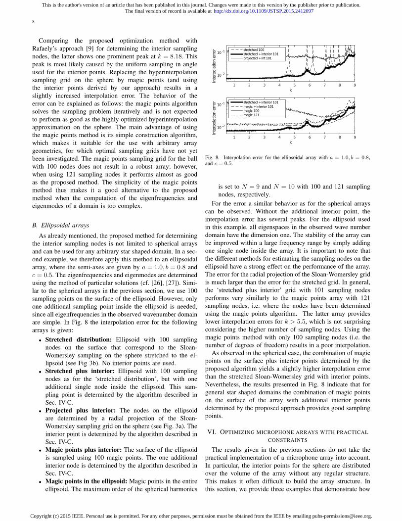
As already mentioned, the proposed method for determiningthe interior sampling nodes is not limited to spherical arraysand can be used for any arbitrary star shaped domain. In a sec-ond example, we therefore apply this method to an ellipsoidalarray, where the semi-axes are given by a = 1.0, b = 0.8 andc = 0.5. The eigenfrequencies and eigenmodes are determinedusing the method of particular solutions (cf. [26], [27]). Simi-lar to the spherical arrays in the previous section, we use 100sampling points on the surface of the ellipsoid. However, onlyone additional sampling point inside the ellipsoid is needed,since all eigenfrequencies in the observed wavenumber domainare simple. In Fig. 8 the interpolation error for the followingarrays is given:• Stretched distribution: Ellipsoid with 100 sampling

nodes on the surface that correspond to the Sloan-Womersley sampling on the sphere stretched to the el-lipsoid (see Fig 3b). No interior points are used.

• Stretched plus interior: Ellipsoid with 100 samplingnodes as for the ‘stretched distribution’, but with oneadditional single node inside the ellipsoid. This sam-pling point is determined by the algorithm described inSec. IV-C.

• Projected plus interior: The nodes on the ellipsoidare determined by a radial projection of the Sloan-Womersley sampling grid on the sphere (see Fig. 3a). Theinterior point is determined by the algorithm described inSec. IV-C.

• Magic points plus interior: The surface of the ellipsoidis sampled using 100 magic points. The one additionalinterior node is determined by the algorithm described inSec. IV-C.

• Magic points in the ellipsoid: Magic points in the entireellipsoid. The maximum order of the spherical harmonics

k

1 2 3 4 5 6 7 8 9

Inte

rpola

tion e

rror

10 -2

10 -1 stretched 100

stretched + interior 101

projected + int 101

k

1 2 3 4 5 6 7 8 9

Inte

rpola

tion e

rror

10 -2

10 -1 stretched + interior 101

magic + interior 101

magic 100

magic 121

Fig. 8. Interpolation error for the ellipsoidal array with a = 1.0, b = 0.8,and c = 0.5.

is set to N = 9 and N = 10 with 100 and 121 samplingnodes, respectively.

For the error a similar behavior as for the spherical arrayscan be observed. Without the additional interior point, theinterpolation error has several peaks. For the ellipsoid usedin this example, all eigenspaces in the observed wave numberdomain have the dimension one. The stability of the array canbe improved within a large frequency range by simply addingone single node inside the array. It is important to note thatthe different methods for estimating the sampling nodes on theellipsoid have a strong effect on the performance of the array.The error for the radial projection of the Sloan-Womersley gridis much larger than the error for the stretched grid. In general,the ‘stretched plus interior’ grid with 101 sampling nodesperforms very similarly to the magic points array with 121sampling nodes, i.e. where the nodes have been determinedusing the magic points algorithm. The latter array provideslower interpolation errors for k > 5.5, which is not surprisingconsidering the higher number of sampling nodes. Using themagic points method with only 100 sampling nodes (i.e. thenumber of degrees of freedom) results in a poor interpolation.

As observed in the spherical case, the combination of magicpoints on the surface plus interior points determined by theproposed algorithm yields a slightly higher interpolation errorthan the stretched Sloan-Womersley grid with interior points.Nevertheless, the results presented in Fig. 8 indicate that forgeneral star shaped domains the combination of magic pointson the surface of the array with additional interior pointsdetermined by the proposed approach provides good samplingpoints.

VI. OPTIMIZING MICROPHONE ARRAYS WITH PRACTICALCONSTRAINTS

The results given in the previous sections do not take thepractical implementation of a microphone array into account.In particular, the interior points for the sphere are distributedover the volume of the array without any regular structure.This makes it often difficult to build the array structure. Inthis section, we provide three examples that demonstrate how



9

to include practical constraints in the optimization of themicrophone array. The first two examples show the design ofspherical arrays, where the interior microphone positions arerestricted to an inner sphere (i.e. an open as well as a closed,sound hard sphere as investigated in [8]). The third exampleoptimizes a spindle torus array, that can be implemented witha simple scanning array as shown in [12].

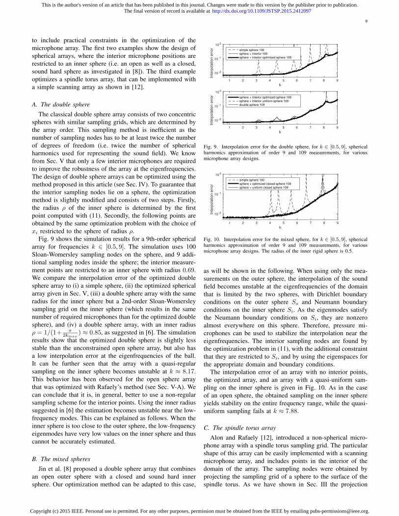
A. The double sphere

The classical double sphere array consists of two concentricspheres with similar sampling grids, which are determined bythe array order. This sampling method is inefficient as thenumber of sampling nodes has to be at least twice the numberof degrees of freedom (i.e. twice the number of sphericalharmonics used for representing the sound field). We knowfrom Sec. V that only a few interior microphones are requiredto improve the robustness of the array at the eigenfrequencies.The design of double sphere arrays can be optimized using themethod proposed in this article (see Sec. IV). To guarantee thatthe interior sampling nodes lie on a sphere, the optimizationmethod is slightly modified and consists of two steps. Firstly,the radius ρ of the inner sphere is determined by the firstpoint computed with (11). Secondly, the following points areobtained by the same optimization problem with the choice ofxi restricted to the sphere of radius ρ.

Fig. 9 shows the simulation results for a 9th-order sphericalarray for frequencies k ∈ [0.5, 9]. The simulation uses 100Sloan-Womersley sampling nodes on the sphere, and 9 addi-tional sampling nodes inside the sphere; the interior measure-ment points are restricted to an inner sphere with radius 0.69.We compare the interpolation error of the optimized doublesphere array to (i) a simple sphere, (ii) the optimized sphericalarray given in Sec. V, (iii) a double sphere array with the sameradius for the inner sphere but a 2nd-order Sloan-Womersleysampling grid on the inner sphere (which results in the samenumber of required microphones than for the optimized doublesphere), and (iv) a double sphere array, with an inner radiusρ = 1/(1+ π

2kmax) ≈ 0.85, as suggested in [6]. The simulation

results show that the optimized double sphere is slightly lessstable than the unconstrained open sphere array, but also hasa low interpolation error at the eigenfrequencies of the ball.It can be further seen that the array with a quasi-regularsampling on the inner sphere becomes unstable at k ≈ 8.17.This behavior has been observed for the open sphere arraythat was optimized with Rafaely’s method (see Sec. V-A). Wecan conclude that it is, in general, better to use a non-regularsampling scheme for the interior points. Using the inner radiussuggested in [6] the estimation becomes unstable near the low-frequency modes. This can be explained as follows. When theinner sphere is too close to the outer sphere, the low-frequencyeigenmodes have very low values on the inner sphere and thuscannot be accurately estimated.

B. The mixed spheres

Jin et al. [8] proposed a double sphere array that combinesan open outer sphere with a closed and sound hard innersphere. Our optimization method can be adapted to this case,

k

1 2 3 4 5 6 7 8 9

Inte

rpo

latio

n e

rro

r

10 -2

10 -1

10 0

simple sphere 100


sphere + interior optimized sphere 109

k

1 2 3 4 5 6 7 8 9

Inte

rpo

latio

n e

rro

r

10 -2

10 -1

10 0

sphere + interior optimized sphere 109

sphere + interior uniform sphere 109

double sphere 109

Fig. 9. Interpolation error for the double sphere, for k ∈ [0.5, 9], sphericalharmonics approximation of order 9 and 109 measurements, for variousmicrophone array designs.

k

1 2 3 4 5 6 7 8 9

Inte

rpola

tion e

rror

10 -2

10 -1

10 0

simple sphere 100

sphere + optimized closed sphere 109

sphere + uniform closed sphere 109

Fig. 10. Interpolation error for the mixed sphere, for k ∈ [0.5, 9], sphericalharmonics approximation of order 9 and 109 measurements, for variousmicrophone array designs. The radius of the inner rigid sphere is 0.5.

as will be shown in the following. When using only the mea-surements on the outer sphere, the interpolation of the soundfield becomes unstable at the eigenfrequencies of the domainthat is limited by the two spheres, with Dirichlet boundaryconditions on the outer sphere So and Neumann boundaryconditions on the inner sphere Si. As the eigenmodes satisfythe Neumann boundary conditions on Si, they are nonzeroalmost everywhere on this sphere. Therefore, pressure mi-crophones can be used to stabilize the interpolation near theeigenfrequencies. The interior sampling nodes are found bythe optimization problem in (11), with the additional constraintthat they are restricted to Si, and by using the eigenspaces forthe appropriate domain and boundary conditions.

The interpolation error of an array with no interior points,the optimized array, and an array with a quasi-uniform sam-pling on the inner sphere is given in Fig. 10. As in the caseof an open sphere, the obtained sampling on the inner sphereyields stability on the entire frequency range, while the quasi-uniform sampling fails at k ≈ 7.88.

C. The spindle torus array

Alon and Rafaely [12], introduced a non-spherical micro-phone array with a spindle torus sampling grid. The particularshape of this array can be easily implemented with a scanningmicrophone array, and includes points in the interior of thedomain of the array. The sampling nodes were obtained byprojecting the sampling grid of a sphere to the surface of thespindle torus. As we have shown in Sec. III the projection



10

k

1 2 3 4 5 6 7 8 9

Inte

rpola

tion e

rror

10 -2

100projected sphere 100

exterior magic points 100

proposed 102

k

1 2 3 4 5 6 7 8 9

Inte

rpola

tion e

rror

10 -2

100magic points 100

magic points 121

proposed 102

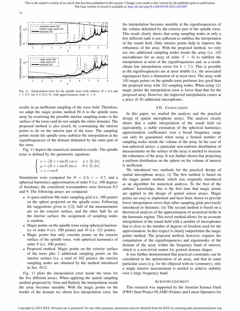
Fig. 11. Interpolation error for the spindle torus with radiuses R = 0.3 andr = 0.7, for k ∈ [0.5, 9], with approximation order L = 9.

results in an inefficient sampling of the wave field. Therefore,we adapt the magic points method IV-A to the spindle torusarray by restricting the possible interior sampling nodes to thesurface of the torus (and do not sample the entire domain). Theproposed method is also tested, by constraining the interiorpoints to lie on the interior part of the torus. The samplingpoints inside the spindle torus stabilize the interpolation at theeigenfrequencies of the domain delimited by the outer part ofthe torus.

Fig. 11 depicts the numerical simulation results. The spindletorus is defined by the parametric equations x = (R+ r sin θ) cosφ φ ∈ [0, 2π[

y = (R+ r sin θ) sinφ θ ∈ [0, 2π[z = r cos θ

Simulations were computed for R = 0.3, r = 0.7, and aspherical harmonics approximation of order 9 (i.e. 100 degreesof freedom); the considered wavenumbers were between 0.5and 9. The following arrays are compared:• A quasi-uniform 9th-order sampling grid (i.e. 100 points)

on the sphere projected on the spindle torus. Followingthe suggestions given in [12], half of the measurementsare on the exterior surface, and the other half lie onthe interior surface; the assignment of sampling nodesis random.

• Magic points on the spindle torus using spherical harmon-ics of order 9 (i.e. 100 points) and 10 (i.e. 121 points).

• Magic points that only consider points on the exteriorsurface of the spindle torus, with spherical harmonics oforder 9 (i.e. 100 points).

• Proposed method: Magic points on the exterior surfaceof the torus plus 2 additional sampling points on theinterior surface (i.e. a total of 102 points); the interiorsampling nodes are obtained by the method introducedin Sec. IV-C.

Fig. 11 plots the interpolation error inside the torus forthe five different arrays. When applying the spatial samplingmethod proposed by Alon and Rafaely the interpolation insidethe array becomes unstable. With the magic points on theborder of the domain we obtain less interpolation error, but

the interpolation becomes unstable at the eigenfrequencies ofthe volume delimited by the exterior part of the spindle torus.This result clearly shows that using sampling nodes at only afew different radii is not sufficient to stabilize the interpolationof the sound field. Only interior points help to improve therobustness of the array. With the proposed method, we onlyuse two additional sampling nodes inside the array (i.e. 102microphones for an array of order N = 9) to stabilize theinterpolation at most of the eigenfrequencies and, as a result,obtain low interpolation errors for k < 7.5. This is possibleas the eigenfrequencies are at most double (i.e. the associatedeigenspaces have a dimension of at most two). The array with100 magic points on the spindle torus performs less good thanthe proposed array with 102 sampling nodes. When using 121magic points the interpolation error is lower than that for theproposed array. However, the improved interpolation comes ata price of 20 additional microphones.

VII. CONCLUSION

In this paper, we studied the analysis and the practicaldesign of spatial microphone arrays. The analysis clearlyshows that a stable interpolation of the sound field (orequivalently, a stable estimation of the spherical harmonicsapproximation coefficients) over a broad frequency rangecan only be guaranteed when using a limited number ofsampling nodes inside the volume of the array. In the case ofnon-spherical arrays, a particular non-uniform distribution ofmeasurements on the surface of the array is needed to increasethe robustness of the array. It was further shown that projectinga uniform distribution on the sphere on the volume of interestis inefficient.

We introduced two methods for the practical design ofspatial microphone arrays: (i) The first method is based onthe magic points method, which was originally introducedas an algorithm for numerical analysis. To the best of theauthors’ knowledge, this is the first time that magic pointsare applied to the design of spatial sensor arrays. Magicpoints are easy to implement and have been shown to providelower interpolation errors than other sampling grids previouslyintroduced in literature. (ii) The second method is based on atheoretical analysis of the approximation of acoustical fields inthe harmonic regime. This novel method allows for an accurateinterpolation of the sound field with a number of microphonesthat is close to the number of degrees of freedom used for theapproximation. In this respect it clearly outperforms the magicpoints method. The proposed method, however, requires thecomputation of the eigenfrequencies and eigenmodes of thedomain of the array within the frequency band of interest,which is a non-trivial matter for general domain shapes.

It was further demonstrated that practical constraints can beconsidered in the optimization of an array, and that in someparticular cases (e.g. for the ellipsoid with no symmetry), onlya single interior measurement is needed to achieve stabilityover a large frequency band.

ACKNOWLEDGMENT

This research was supported by the Austrian Science Fund(FWF) Start Project FLAME (Frames and Linear Operators for



11

Acoustical Modeling and Parameter Estimation; Y 551-N13),the French ANR CONTINT project SOR2 (Sample Orches-trator 2), and the S&T cooperation project Amadeus Austria-France 2013-14, “Frame Theory for Sound Processing andAcoustic Holophony”, FR 16/2013.

REFERENCES

[1] T. D. Abhayapala and D. B. Ward, “Theory and design of high ordersound field microphones using spherical microphone array,” in Acoustics,Speech and Signal Processing (ICASSP), IEEE International Conferenceon, 2002, pp. 1949–1952.

[2] B. N. Gover, J. G. Ryan, and M. R. Stinson, “Measurements ofdirectional properties of reverberant sound fields in rooms using aspherical microphone array,” The Journal of the Acoustical Society ofAmerica, vol. 116, no. 4, pp. 2138–2148, 2004.

[3] J. Meyer and G. W. Elko, “A highly scalable spherical microphone arraybased on an orthonormal decomposition of the soundfield,” in Acoustics,Speech and Signal Processing (ICASSP), IEEE International Conferenceon, 2002, pp. 1781–1784.

[4] T. Rahim and D. E. N. Davies, “Effect of directional elements on thedirectional response of circular antenna arrays,” in Microwaves, Opticsand Antennas, IEE Proceedings H, 1982, pp. 18–22.

[5] J. Meyer, “Beamforming for a circular microphone array mounted onspherically shaped objects,” The Journal of the Acoustical Society ofAmerica, vol. 109, no. 1, pp. 185–193, 2001.

[6] I. Balmages and B. Rafaely, “Open-sphere designs for spherical mi-crophone arrays,” IEEE Transactions on Audio, Speech and LanguageProcessing, vol. 15, no. 2, pp. 727–732, 2007.

[7] A. Parthy, C. T. Jin, and A. van Schaik, “Acoustic holography witha concentric rigid and open spherical microphone array,” in Acoustics,Speech and Signal Processing (ICASSP), IEEE International Conferenceon, 2009, pp. 2173–2176.

[8] C. T. Jin, N. Epain, and A. Parthy, “Design, optimization and evalua-tion of a dual-radius spherical microphone array,” Audio, Speech, andLanguage Processing, IEEE/ACM Transactions on, vol. 22, no. 1, pp.193–204, Jan 2014.

[9] B. Rafaely, “The spherical-shell microphone array,” IEEE Transactionson Audio, Speech and Language Processing, vol. 16, no. 4, pp. 740–747,May 2008.

[10] T. D. Abhayapala and A. Gupta, “Alternatives to spherical microphonearrays: Hybrid geometries,” in Acoustics, Speech and Signal Processing(ICASSP), IEEE International Conference on, Apr. 2009, pp. 81–84.

[11] A. Gupta and T. D. Abhayapala, “Double sided cone array for sphericalharmonic analysis of wavefields,” in Acoustics, Speech and SignalProcessing (ICASSP), IEEE International Conference on, 2010, pp. 77–80.

[12] D. L. Alon and B. Rafaely, “Spindle-torus sampling for an efficient-scanning spherical microphone array,” Acta Acustica United With Acus-tica, vol. 98, no. 1, pp. 83–90, Jan. 2012.

[13] R. Mignot, G. Chardon, and L. Daudet, “Low frequency interpolationof room impulse responses using compressed sensing,” IEEE/ACMTransactions on Audio, Speech and Language Processing (TASLP),vol. 22, no. 1, pp. 205–216, 2014.

[14] B. Rafaely, “Bessel nulls recovery in spherical microphone arrays fortime-limited signals,” Audio, Speech, and Language Processing, IEEETransactions on, vol. 19, no. 8, pp. 2430–2438, 2011.

[15] G. Chardon, W. Kreuzer, and M. Noisternig, “Design of a robust openspherical microphone array,” in Acoustics, Speech and Signal Processing(ICASSP), 2014 IEEE International Conference on, Florence, Italy, May2014, pp. 6860–6863.

[16] H. L. Van Trees, Optimum Array Processing, ser. Part IV of Detection,Estimation, and Modulation Theory. Wiley Interscience, 2002.

[17] A. Moiola, R. Hiptmair, and I. Perugia, “Plane wave approximation ofhomogeneous Helmholtz solutions,” Zeitschrift fur Angewandte Mathe-matik und Physik (ZAMP), vol. 62, pp. 809–837, 2011.

[18] J. Melenk, “Operator adapted spectral element methods I: harmonic andgeneralized harmonic polynomials,” Numerische Mathematik, vol. 84,pp. 35–69, 1999.

[19] C. Runge, “Uber empirische Funktionen und die Interpolation zwischenaquidistanten Ordinaten,” Zeitschrift fur Mathematik und Physik, vol. 46,pp. 224–243, 1901.

[20] A. Cohen, M. A. Davenport, and D. Leviatan, “On the stability and ac-curacy of least squares approximations,” Foundations of ComputationalMathematics, vol. 13, no. 5, pp. 819–834, 2013.

[21] G. Chardon, A. Cohen, and L. Daudet, “Reconstruction of solutionsto the Helmholtz equation from punctual measurements,” in 10th In-ternational Conference on Sampling Theory and Applications, Bremen,Germany, Jul. 2013.

[22] ——, “Sampling and reconstruction of solutions to the Helmholtzequation,” Sampling Theory in Signal and Image Processing, vol. 13,no. 1, pp. 67–89, 2014.

[23] I. H. Sloan and R. S. Womersley, “The Uniform Error of Hyperinter-polation on the Sphere,” in Advances in Multivariate Approximation,W. Haußmann, K. Jetter, and M. Reimer, Eds. Witten-Bommerholz,Germany: Wiley-VCH Verlag, 1998, pp. 289–306.

[24] R. Womersley and I. Sloan, “How good can polynomial interpolationon the sphere be?” Advances In Computational Mathematics, vol. 14,no. 3, pp. 195–226, 2001.

[25] Y. Maday, N. Nguyen, A. Patera, and G. Pau, “A general multipurposeinterpolation procedure: The magic points,” Comm. Pure Appl. Math.,vol. 8, no. 1, pp. 383–404, 2009.

[26] A. H. Barnett, “Dissipation in deforming chaotic billiards,” Ph.D.dissertation, Harvard University, 2000.

[27] T. Betcke and L. Trefethen, “Reviving the method of particular solu-tions,” SIAM review, pp. 469–491, 2005.

Gilles Chardon received the engineering degreesof the Ecole Polytechnique and Telecom ParisTechin 2009, as well as the MSc ATIAM of UniversitePierre et Marie Curie, Paris VI. After working to-wards his PhD at Institut Langevin in Paris, anda postdoctoral position with the Mathematics andSignal Processing group of the Acoustics ResearchInstitute of the Austrian Academy of Sciences inVienna, he is now Associate Professor with Centrale-Supelec, Gif-sur-Yvette, France. His main researchinterests include sparse representation of acoustical

fields, inverse problems and numerical analysis in acoustics.

Wolfgang Kreuzer received his Ph.D in engineeringmathematics in 2000 at the Technical University ofVienna. After working at the Institute for Appliedand Numerical Mathematics at the TU-Vienna hejoined the Acoustics Research Institute of the Aus-trian Academy of Sciences in 2004. His main re-search interests is focused on models and simulationof wave propagation and wave scattering.

Markus Noisternig obtained his MSc degree inElectrical Engineering and Audio Engineering fromthe University of Technology (TUG) and the Univer-sity of Music and Performing Arts (KUG) Graz in2003. From 2003 to 2007 he was a Research Scien-tist at the Institute of Electronic Music and Acoustics(IEM) working towards his PhD. In 2007 he wasresearcher at the LIMSI-CNRS and since 2008, hehas been a Researcher at the UMR IRCAM-CNRS-UPMC in Paris. He is also Senior Lecturer at theIEM and lectures at the Hochschule fur Gestaltung

in Karlsruhe. Taking both an artistic and scientific interest in matters of soundand music, he also studied computer music composition at the KUG.



Design of spatial microphone arrays for sound field ...

Documents

Transcript of Design of spatial microphone arrays for sound field ...