
Design of Resilient Smart Highway Systems with Data-Driven ...
44
New York University Rutgers University University of Washington The University of Texas at El Paso City College of New York A USDOT University Transportation Center Design of Resilient Smart Highway Systems with Data- Driven Monitoring from Networked Cameras August 2020
Transcript of Design of Resilient Smart Highway Systems with Data-Driven ...
New York University
Rutgers University
University of Washington
The University of Texas at El Paso
City College of New York A USDOT University Transportation Center
Design of Resilient Smart Highway Systems with Data-
Driven Monitoring from Networked Cameras
August 2020

Error! No text of specified style in document. ii
Design of Resilient Smart Highway Systems with Data-Driven Monitoring from Networked Cameras
Principal Investigator: Li Jin
New York University
ORC-ID: 0000-0002-5282-2327
Co PI: Chen Feng
New York University
ORC-ID: 0000-0003-3211-1576
Student: Qian Xie
New York University
Student: Xuchu Xu
New York University
C2SMART Center is a USDOT Tier 1 University Transportation Center taking on some of today’s most pressing urban mobility challenges. Some of the areas C2SMART focuses on include:
Urban Mobility and Connected Citizens
Urban Analytics for Smart Cities
Resilient, Smart, & Secure Infrastructure
Disruptive Technologies and their impacts on transportation systems. Our aim is to develop innovative solutions to accelerate technology transfer from the research phase to the real world.
Unconventional Big Data Applications from field tests and non-traditional sensing technologies for decision-makers to address a wide range of urban mobility problems with the best information available.
Impactful Engagement overcoming institutional barriers to innovation to hear and meet the needs of city and state stakeholders, including government agencies, policy makers, the private sector, non-profit organizations, and entrepreneurs.
Forward-thinking Training and Development dedicated to training the workforce of tomorrow to deal with new mobility problems in ways that are not covered in existing transportation curricula.
Led by New York University’s Tandon School of Engineering, C2SMART is a consortium of leading research universities, including Rutgers

Design of Resilient Smart Highway Systems with Data-Driven Monitoring from Networked Cameras iii
University, University of Washington, the University of Texas at El Paso, and The City College of NY.
Visit c2smart.engineering.nyu.edu to learn more

Design of Resilient Smart Highway Systems with Data-Driven Monitoring from Networked Cameras iv
Disclaimer The contents of this report reflect the views of the authors, who are responsible for the facts and the accuracy of the information presented herein. This document is disseminated in the interest of information exchange. The report is funded, partially or entirely, by a grant from the U.S. Department of Transportation’s University Transportation Centers Program. However, the U.S. Government assumes no liability for the contents or use thereof.
Acknowledgements We appreciate the support from the US Department of Transportation, the NYU Tandon School of Engineering faculty startup funds, and the NYU Undergraduate Summer Research Internship program. Undergraduate students including Aiqi Zhou, Martin Buceta, Ziyan An, Eric Gan, and Weiyao Xie also contributed to this project. We also appreciate the discussion with Prof. Kaan Ozbay and the assistance from Shri Iyer, Joseph C. Williams, and John Petinos.

Design of Resilient Smart Highway Systems with Data-Driven Monitoring from Networked Cameras v
Executive Summary This project aims to develop a systematic way to design smart highway systems with networked video monitoring and control resiliency against environment disruptions and sensor failures. On the video monitoring side, we investigate 1) efficient deep learning methods for extracting fine-grained local categorical traffic information from individual surveillance videos (e.g., traffic mixture, environment information, anomaly/extreme-weather detection in the scene), and 2) machine learning-based methods to correlate and propagate the local information through the highway network for global states estimation (e.g., vehicle tracking and reidentification, traffic prediction in unobserved area). On the system design side, we 1) establish dynamic models for capacity using video data, 2) model failure in either cyber or physical components, 3) study the relation between sensor deployment and observability for resilient traffic control (e.g. route guidance and ramp metering). The outcome is an implementable approach to designing resilient smart highway systems with trustworthy monitoring capability. We also expect our approach (with appropriate modification) to be applicable to general transportation systems.

Design of Resilient Smart Highway Systems with Data-Driven Monitoring from Networked Cameras vi
Table of Contents Executive Summary ............................................................................................................................. v Table of Contents ............................................................................................................................... vi List of Figures..................................................................................................................................... vii List of Tables ...................................................................................................................................... vii Section 1: Introduction ........................................................................................................................ 1
Subsection 1.1 Learning-based monitoring ........................................................................ 1 Subsection 1.2 Fault-tolerant traffic control ...................................................................... 4
Section 2: Literature Review ............................................................................................................... 6 Subsection 2.1 Learning-based identification..................................................................... 6 Subsection 2.2: Fault-tolerant traffic control ..................................................................... 6
Section 3: Multi-source data imputation ............................................................................................ 7 Subsection 3.1 Overview .................................................................................................... 7 Subsection 3.2 Compressive MHE ...................................................................................... 8 Subsection 3.3 Theoretical Insights .................................................................................. 11 Subsection 3.4 Experiments & Results ............................................................................. 14 Subsection 3.5 Concluding remarks .................................................................................. 20
Section 4: Traffic control under faulty sensing ................................................................................. 21 Subsection 4.1: Introduction............................................................................................. 21 Subsection 4.2: Modeling ................................................................................................. 21 Subsection 4.2: Analysis .................................................................................................... 23 Subsection 4.3: Results ..................................................................................................... 27 Subsection 4.4: Extension to general networks ............................................................... 29 Subsection 4.5: Subsequent work: Simulation of I210 ..................................................... 30
Section 5: Conclusions ....................................................................................................................... 31 References ......................................................................................................................................... 32

Design of Resilient Smart Highway Systems with Data-Driven Monitoring from Networked Cameras vii
List of Figures Figure 3.1: Comparison of original MHE and compressive MHE. .................................................. 2 Figure 3.2: Hyperspherical energy during training. ..................................................................... 17 Figure 3.3: Visualized first-layer filters. ...................................................................................... 19 Figure 4.1: Selection over parallel routes. .................................................................................. 21 Figure 4.2: Two parallel routes (left) with four failure modes (right). .......................................... 22 Figure 4.3: Illustration of the continuous state process and the invariant set 𝑴. The arrows represent the vector field 𝑮 defined in (7) for the four states. ................................................... 24 Figure 4.4: Impact of link failure probability (𝝆 = 𝟎) and link failure correlation (𝒑 = 𝟎. 𝟓) on the lower bound of resilience score. .......................................................................................... 28 Figure 4.5: Network structure. ................................................................................................... 29 Figure 4.6: Simulation testbed for I210 near Los Angeles. .......................................................... 30
List of Tables Table 3.1: CoMHE variants on C-100. ......................................................................................... 14 Table 3.2: Error (%) on CIFAR-100 under different dimension of projection. ............................... 15 Table 3.3: Error (%) on CIFAR-100 under different numbers of projections. ............................... 16 Table 3.4: Error (%) on CIFAR-100 with different network width. ............................................... 16 Table 3.5: Error on CIFAR-100 with different network depth. N/C denotes Not Converged. ........ 17 Table 3.6: Error (%) using ResNets. ............................................................................................ 18 Table 3. 7: Top-1 center crop error on ImageNet. ...................................................................... 18 Table 3.8: Accuracy (%) on ModelNet-40. .................................................................................. 19 Table 4.1: Nominal model parameters ....................................................................................... 27
Design of Resilient Smart Highway Systems with Data-Driven Monitoring from Networked Cameras 1
Section 1: Introduction The growing deployment of surveillance cameras in highway systems can provide system operators with richer information such as weather, incidents, and other traffic-disrupting events, which conventional sensors (e.g. loop inductors) cannot provide. However, two important questions have to be addressed before extensive implementation. First, how to accurately and robustly retrieve relevant information from not only an individual camera but networked cameras, especially fine-grained vehicle recognition and tracking, anomaly detection, and predictions in unobserved areas. Second, how to design a resilient control system that maximizes the use of camera data while minimizing the negative impact of sensor failures and error in data processing. These questions have to be jointly addressed, since the performance of automatic video monitoring, the deployment (number and locations) of surveillance cameras, and traffic control algorithm based on real-time information are closely related and interdependent.
For the monitoring part, thanks to the recent development of deep learning techniques, especially convolutional neural networks (CNN), accurate, robust, and efficient object detection in images and videos has become more accessible, e.g., state-of-the-art CNN architectures like Fast-RCNN/SSD/Yolo/Mask-RCNN provide strong algorithm backbones to address the traditional challenges such as partial occlusion, cluttered scene, etc. However, most existing data-driven methods focus on traffic monitoring from single cameras. Very recently, researchers started to investigate data-driven analysis of networked videos for traffic analysis. However, these methods do not systematically take a transportation network structure into consideration using a data-driven approach.
For the system design part, although numerous efforts have been devoted to design of performance-improving traffic control systems, the existing approaches typically assume deterministic environment (demand/capacity) and fully functional sensors. This project considers a more realistic setting where the environment is subject to disruptions and the sensors (cameras) are subject to failures.
Subsection 1.1 Learning-based monitoring
Recent years have witnessed the tremendous success of deep neural networks in a variety of tasks. With its over-parameterization nature and hierarchical structure, deep neural networks achieve unprecedented performance on many challenging problems [1, 2, 3], but their strong ap- proximation ability also makes it easy to overfit the training set, which greatly affects the generalization on unseen samples. Therefore, how to restrict the huge parameter space and properly regularize the deep networks becomes increasingly important. Regularizations for neural networks can be roughly categorized into implicit and explicit ones. Implicit regularizations usually do not directly impose explicit constraints on neuron weights, and instead they regularize the networks in an implicit manner in order to prevent overfit- ting and stabilize the training. A lot of prevailing methods fall into this category, such as batch normalization [4], dropout [5], weight normalization [6], etc. Explicit regularizations [7, 8, 9, 10, 11, 12] usually introduce some penalty terms for neuron weights, and jointly optimize them along with the other objective functions.

Design of Resilient Smart Highway Systems with Data-Driven Monitoring from Networked Cameras 2
Figure 1.1: Comparison of original MHE and compressive MHE.
Among many existing explicit regularizations, minimum hyperspherical energy (MHE) [12] stands out as a simple yet effective regularization that promotes the hyperspherical diversity among neurons and significantly improves the network generalization. MHE regularizes the directions of neuron weights by minimizing a potential energy on a unit hypersphere that characterizes the hyperspherical diversity (such energy is defined as hyperspherical energy [12]). In contrast, standard weight decay only regularizes the norm of neuron weights, which essentially can be viewed as regularizing one dimension of the weights. MHE completes an important missing piece by regularizing the neuron directions (i.e., regularizing the rest dimensions of the weights).
Although minimizing hyperspherical energy has already been empirically shown useful in a number of applications [12], two fundamental questions remain unanswered:(1) what is the role that hyperspherical energy plays in training a well-performing neural network? and (2) How can the hyperspherical energy be effectively minimized? To study the first question, we plot the training dynamics of hyperspherical energy (on CIFAR-100) in Figure 1.1(c) for a baseline convolutional neural network (CNN) without any MHE variant, a CNN regularized by MHE [12] and a CNN regularized by our CoMHE. From the empirical results in Figure 1.1(c), we find that both MHE and CoMHE can achieve much lower hyperspherical energy and testing error than the baseline, showing the effectiveness of minimizing hyperspherical energy. It also implies that lower hyperspherical energy typically leads to better generalization. We empirically observe that a trained neural network with lower hyperspherical energy often generalizes better (i.e., higher hyperspherical diversity leads to better generalization), and therefore we argue that hyperspherical energy is closely related to the generalization power of neural networks. In the rest of the paper, we delve into the second question that remains an open challenge: how to effectively minimize hyperspherical energy.
By adopting the definition of hyperspherical energy as the regularization objective and naively minimizing it with back-propagation, MHE suffers from a few critical problems which limit it to further unleash its potential. First, the original MHE objective has a huge number of local minima and stationary points due to its highly non-convex and non-linear objective

Design of Resilient Smart Highway Systems with Data-Driven Monitoring from Networked Cameras 3
function. The problem can get even worse when the space dimension gets higher and the number of neurons becomes larger [13, 14]. Second, the gradient of the original MHE objective w.r.t the neuron weight is deterministic. Unlike the weight decay whose objective is convex, MHE has a complex and non-convex regularization term. Therefore, deterministic gradients may make the solution quickly fall into one of the bad local minima and get stuck there. Third, MHE defines an ill-posed problem in general. When the number of neurons is smaller than the dimension of the space (it is often the case in neural net- works), it will be less meaningful to encourage the hyper- spherical diversity since the neurons cannot fully occupy the space. Last, in high-dimensional spaces, randomly initialized neurons are likely to be orthogonal to each other. Therefore, these high-dimensional neurons can be trivially “diverse”, leading to small gradients in original MHE that cause optimization difficulties.
In order to address these problems and effectively minimize hyperspherical energy, we propose the compressive minimum hyperspherical energy (CoMHE) as a generic regularization for neural networks. The high-level intuition behind CoMHE is to project neurons to some suitable subspaces such that the hyperspherical energy can get minimized more effectively. Specifically, CoMHE first maps the neurons from a high-dimensional space to a low- dimensional one and then minimizes the hyperspherical energy of these neurons. Therefore, how to map these neuons to a low-dimensional space while preserving the desirable information in high-dimensional space is our major concern. Since we aim to regularize the directions of neurons, what we care most is the angular similarity between different neurons. To this end, we explore multiple novel methods to perform the projection and heavily study two main approaches: random projection and angle-preserving projection, which can reduce the dimensionality of neurons while still partially preserving the pairwise angles.
Random projection (RP) is a natural choice to perform the dimensionality reduction in MHE due to its simplicity and nice theoretical properties. RP can provably preserve the angular information, and most importantly, introduce certain degree of randomness to the gradients, which may help CoMHE escape from some bad local minima. The role that the randomness serves in CoMHE is actually similar to the simulated annealing [15, 16] that is widely used to solve Thomson problem. Such randomness is often shown to benefit the generalization [17, 18]. We also provably show that using RP can well preserve the pairwise angles between neurons. Besides RP, we propose the angle-preserving projection (AP) as an effective alternative. AP is motivated by the goal that we aim to preserve the pairwise angles between neurons. Constructing an AP that can project neurons to a low-dimensional space that well preserves the angles is of- ten difficult even with powerful non-linear functions, which is suggested by the strong conditions required for conformal mapping in complex analysis [19]. Therefore, we frame the AP construction as an optimization problem which can be solved jointly with hyperspherical energy minimization. More interestingly, we consider the adversarial projection for CoMHE, which minimizes the maximal energy attained by learning the projection. We formulate it as a min-max optimization and optimize it jointly with the neural network.
However, it is inevitable to lose some information in low-dimensional spaces and the neurons may only get diverse in some low-dimensional spaces. To address it, we adopt multiple projections to better approximate the MHE objective in the original high-dimensional space. Specifically, we project the neurons to multiple subspaces, compute the hyperspherical energy

Design of Resilient Smart Highway Systems with Data-Driven Monitoring from Networked Cameras 4
in each space separately and then minimize the aggregation (i.e., average or max). Moreover, we reinitialize these projection matrices randomly every certain number of iterations to avoid trivial solutions.
In contrast to MHE that imposes a static regularization to the neurons, CoMHE dynamically regularizes the neurons based on the projection matrices. Such dynamic regularization is equivalent to adjusting the CoMHE objective function, making it easier to escape some bad local minima. Our contributions can be summarized as:
• We first show that hyperspherical energy is closely related to generalization and then reveal the role it plays in training a neural network that generalizes well.
• To address the drawbacks of MHE, we propose CoMHE as a dynamic regularization to effectively minimize hyperspherical energy of neurons for better generalizability.
• We explore different ways to construct a suitable projection for CoMHE. Random projection and angle-preserving projection are proposed to reduce the dimensionality of neurons while preserving the angular information. We also consider several variants such as adversarial projection CoMHE and group CoMHE.
• We provide some theoretical insights for the proposed projections on the quality of preserving the angular similarity between different neurons.
• We show that CoMHE consistently outperforms the original MHE in different tasks. Notably, a 9-layer plain CNN regularized by CoMHE outperforms a standard1001-layer ResNet by more than 2% on CIFAR-100.
Subsection 1.2 Fault-tolerant traffic control
The rapidly growing deployment of traffic sensing and vehicle-to-vehicle/infrastructure (V2V/ V2I) communications has enabled the concept of intelligent transportation system (ITS). In ITS, system operators and travelers have access to real-time traffic conditions and can thus make better decisions. Dynamic routing is a typical ITS capability, which is conducted via route guidance tools such as Google Maps and WAZE. System operators can also influence routing via tolling and instructions for traffic diversion, which also rely on real-time traffic conditions. A major challenge for dynamic routing in ITS is how to ensure system functionality and efficiency under a variety of sensing faults. Quality of sensing and communications significantly affects system performance. However, data health is a serious issue that system operators must face. On some highways, up to 30%-40% of loop sensors do not report accurate measurements [1, 2]; similar issue exists for camera sensors. Even though some routing guidance tools may have certain internal fault detection and correction actions, the benefits of such actions can be further evaluated. Moreover, without appropriate fault-tolerant mechanisms, feedback control algorithms may make decisions based on wrong information, and ITS may even perform worse than a comparable conventional transportation system. Therefore, ITS will not be well accepted by the public and transportation authorities unless the impact of sensing faults is adequately evaluated and addressed. However, such impact has not been well understood, and practically relevant fault-tolerant routing algorithms have not been developed.

Design of Resilient Smart Highway Systems with Data-Driven Monitoring from Networked Cameras 5
Our modeling approach is innovative in that we model the occurrence and clearance of sensing faults as a finite-state, continuous-time Markov process. If the sensing on a link is normal, travelers know the true traffic state (traffic density) on the link. If the sensing is faulty, the traffic state will appear to be zero to the travelers. Besides such denial-of-service, our modeling approach can also be extended to incorporate other forms of sensing faults, such as bias and distortion. We adopt the classical logit model [15] for routing; the essential principle of this model is that more traffic will go to a less congested link. When the sensing on a link is faulty, travelers may mistakenly consider a congested link to be uncongested. We show that such faulty information may affect the network’s throughput. The discrete states of the Markov process are essentially modes for the flow dynamics, which govern the evolution of the continuous states. Hence, our model belongs to a class of stochastic processes called piecewise-deterministic Markov processes [16, 17]. Similar models have been used for demand/capacity fluctuations [18, 19]; this paper extends the modeling approach to sensing faults.
A key step for resilience analysis is to determine the stability of the traffic densities under various combinations of parameters. We study the stability of the network based on the theory of continuous-time Markov processes [20]. We derive a necessary condition for stability by constructing a positively invariant set for the dynamic flow network. We derive a sufficient condition by considering a quadratic, switched Lyapunov function that verifies the Foster-Lyapunov drift condition. We exploit a special property of the flow dynamics, called cooperative dynamics [21, 22], to derive an easy-to-check stability criterion, which states that the network is stable if there exists a queuing state such that the rate of change of the fastest growing queue averaged over the modes is negative. Based on the stability analysis, we analyze the network’s throughput (resilience score). We define throughput as the maximal inflow that the network can take while maintaining stable. As a baseline, we first study the behavior of the network if both links have the same flow functions. We perturb the baseline in multiple dimensions (probability and correlation of sensing faults on two links) and analyze how throughput can be affected. We also show that throughput reduces as the two link’s asymmetry increases.
The main contributions of this project include
• A novel stochastic model for sensing fault-prone transportation networks,
• Easy-to-check stability conditions for the network, and
• Resilience analysis under various settings.
Design of Resilient Smart Highway Systems with Data-Driven Monitoring from Networked Cameras 6
Section 2: Literature Review Subsection 2.1 Learning-based monitoring Diversity-based regularization has been found useful in sparse coding (Mairal et al. 09, Ramirez et al. 10), ensemble learning (Li et al. 12, Knuncheva & Whitaker 03), self-paced learning (Jiang et al. 14), metric learning (Xie et al. 18), latent variable models (Xie et al. 16), etc. Early studies in sparse coding (Mairal et al. 09, Ramirez et al. 10) model the diversity with the empirical covariance matrix and show that encouraging such diversity can improve the dictionary's generalizability (Xie et al. 17) promotes the uniformity among eigenvalues of the component matrix in a latent space model (Cogswell 16, Rodriguez 17, Xie et al. 17) characterize diversity among neurons with orthogonality, and regularize the neural network by promoting the orthogonality. Inspired by the Thomson problem in physics, MHE (Liu et al. 18) defines the hyperspherical energy to characterize the diversity on a unit hypersphere and shows significant and consistent improvement in supervised learning tasks. There are two MHE variants in (Liu et al. 18): full-space MHE and half-space MHE. Compared to full-space MHE, the half-space variant further eliminates the collinear redundancy by constructing virtual neurons with the opposite direction to the original ones and then minimizing their hyperspherical energy together. The importance of regularizing angular information is also discussed in (Liu et al. 16, Deng et al. 18, Wang et al. 18).
Subsection 2.2: Fault-tolerant traffic control Existing model-based traffic management approaches typically assume complete knowledge of the traffic condition (Gomes & Horowitz 06, Coogan & Arcak 15, Reilly et al. 15, Yu & Krstic 19), but feedback traffic management for ITS in the face of sensing faults has not been well studied. Como et al. (12) studied the resilience of distributed routing in the face of physical disruptions to link capacities in a dynamic flow network. Lygeros et al. (00) proposed a conceptual framework for fault-tolerant traffic management, but the concrete algorithms are still yet to be developed. A body of work on fault-tolerant control has been developed for a class of dynamical systems (Patton 97, Blanke et al. 06, Zhang & Jiang 08). However, very limited results are available for recurrent and random faults. In addition, there exist some results on adaptive/learning-based fault-tolerant control with applications in electrical/mechanical/aerospace engineering (Zhang et al. 04, Mhaskar et al. 06, Tang et al. 07), but these results are not directly applicable to ITS, nor do they explicitly consider stochastic sensing faults.
Design of Resilient Smart Highway Systems with Data-Driven Monitoring from Networked Cameras 7
Section 3: Multi-source data imputation Subsection 3.1 Overview
We have investigated multiple deep neural network architecture designs and significantly improved the computer-vision-based vehicle detection and counting’s efficiency and accuracy and updated the software prototype code for better visualization of the results. We also tested the performance on various weather conditions including raining. The investigation results demonstrated effectiveness of tracking and counting vehicles from existing traffic cameras. The experimental results not only showed that the overall vision-based vehicle counting performance is comparable to that of loop-detector-based method, but also showed that extra detail traffic statistics such as categorical vehicle counting (truck vs. car) is achievable now. Meanwhile, the investigation revealed several practical challenges in state-of-the-art vision-based object detection and tracking algorithms that results in inaccurate vehicle detection and counting. This includes both the various resolutions and mounting setups of real-world traffic camera images that leading to different vehicle size and visual features in the captured images, and also inconsistent sampling rate across different traffic cameras among which some often have non-smooth video stream or large time gaps between neighboring frames that challenges existing object tracking methods. This shows that to apply existing computer vision object detection and tracking algorithms that are usually designed and trained on datasets collected in self-driving scenes are not necessarily optimal for traffic video analysis from a transportation engineering perspective. A custom, human annotated, large-scale dataset focusing on traffic video collected from traffic cameras would greatly improve the performance and is recommended for future projects on the same topic. This effort has trained a team of two graduate students and four senior students from computer science to attend a closely related public vision-based transportation video analysis competition.
As mentioned above, deep neural network is the most fundamental building block that ensures the good performance of a data-driven monitoring system based on networked cameras or other sensors (e.g., Lidars). Current deep networks for 2D/3D object detection or tracking are usually trained by cross-entropy loss and L2 loss with simple L2-based regularization of the network parameters. To improve the network’s generalization performance when tested on traffic surveillance data, we need to improve the network regularization method. Inspired by the Thomson problem in physics where the distribution of multiple propelling electrons on a unit sphere can be modeled via minimizing some potential energy, hyperspherical energy minimization has demonstrated its potential in regularizing neural networks and improving their generalization power. In this section, we first study the important role that hyperspherical energy plays in neural network training by analyzing its training dynamics. Then we show that naively minimizing hyperspherical energy suffers from some difficulties due to highly non-linear and non-convex optimization as the space dimensionality becomes higher, therefore limiting the potential to further improve the generalization. To address these problems, we propose the compressive minimum hyperspherical energy (CoMHE) as a more effective regularization for neural networks. Specifically, CoMHE utilizes projection mappings to reduce the dimensionality of neurons and minimizes their hyperspherical energy. According to different designs for the projection mapping, we propose several distinct yet well-performing variants and provide some
Design of Resilient Smart Highway Systems with Data-Driven Monitoring from Networked Cameras 8
theoretical guarantees to justify their effectiveness. Our experiments show that CoMHE consistently outperforms existing regularization methods, and can be easily applied to different neural networks.
Subsection 3.2 Compressive MHE
Revisiting Standard MHE
MHE characterizes the diversity of N neurons ( 𝑊𝑁 = {𝑤1,⋯ ,𝑤𝑁 ∈ ℝ𝑑+1} ) on a unit hypersphere using hyperspherical energy which is defined as
𝐸𝑠,𝑑(�̂�𝑖|𝑖=1𝑁 ) = ∑ ∑ 𝑓𝑠
𝑁
𝑗=1,𝑗≠𝑖
𝑁
𝑖=1
(‖�̂�𝑖 − �̂�𝑗‖)
= {∑ ‖�̂�𝑖 − �̂�𝑗‖
−𝑠𝑖≠𝑗 , 𝑠 > 0
∑ 𝑙𝑜𝑔(‖�̂�𝑖 − �̂�𝑗‖−1
)𝑖≠𝑗 , 𝑠 = 0 (1)
where ‖⋅‖ denotes 𝑙2 norm, 𝑓𝑠(⋅)is a decreasing realvalued function(we use 𝑓𝑠(𝑧) = 𝑧−𝑠, 𝑠 >0,i.e., Riesz s-kernels), and �̂�𝑖 = 𝑤𝑖/‖𝑤𝑖‖ is the i-th neuron weight projected onto the unit
hypersphere 𝕊𝑑 = {𝑣 ∈ ℝ𝑑+1 ∣ ‖𝑣‖ = 1}. For convenience, we denote �̂�𝑁 = {�̂�1,⋯ , �̂�𝑁 ∈
𝕊𝑑}, and 𝐸𝑠 = 𝐸𝑠,𝑑(�̂�𝑖|𝑖=1𝑁 ). Note that, each neuron is a convolution kernel in CNNs. MHE
minimizes the hyperspherical energy of neurons using gradient descent during back-propagation, and MHE is typically applied to the neural network in a layer-wise fashion. We first write down the gradient of E2 w.r.t �̂�𝑖 and make the gradient to be zero:
𝛻�̂�𝑖𝐸2 = ∑
−2(�̂�𝑖−�̂�𝑗)
‖�̂�𝑖−�̂�𝑗‖4
𝑁𝑗=1,𝑗≠𝑖 = 0 ⇒ �̂�𝑖 =
∑ 𝛼𝑗𝑁𝑗=1,𝑗≠𝑖 �̂�𝑗
∑ 𝛼𝑗𝑁𝑗=1,𝑗≠𝑖
(2)
where 𝛼𝑗 = ‖�̂�𝑖 − �̂�𝑗‖−4
. We use toy and informal examples to show that high dimensional
space (i.e, d is large) leads to much more stationary points than low-dimensional one. Assume
there are 𝐾 = 𝐾1 + 𝐾2 stationary points in total for �̂�𝑁 to satisfy Eq.2, where 𝐾1 denotes the number of stationary points in which every element in the solution is distinct and 𝐾2 denotes the number of the rest stationary points. We give two examples: (i) For(d+2)-dimensional space, we can extend the solutions in(d+1)-dimensional space by introducing a new dimension with zero value. The new solutions satisfy Eq.2. Because there are d+2 ways to insert the zero,
we have at least(d+2)K stationary points in (d+2)-dimensional space.(ii) We denote 𝐾1′ =
𝐾1
(𝑑+1)!
as the number of unordered sets that construct the stationary points. In(2d+2)-dimensional
space, we can construct �̂�𝑗𝐸 =
1
√2{�̂�𝑗; �̂�𝑗} ∈ 𝕊2𝑑+1, ∀𝑗 that satisfies Eq.2. Therefore, there are
at least (2𝑑+2)!
2𝑑+1 𝐾1′ + 𝐾2 stationary points for �̂�𝑁 in(2d+2)-dimensional space, and besides this
construction, there are much more stationary points. Therefore, MHE have far more stationary points in higher dimensions.

Design of Resilient Smart Highway Systems with Data-Driven Monitoring from Networked Cameras 9
General Framework
To overcome MHE's drawbacks in high dimensional space, we propose the compressive MHE that projects the neurons to a low-dimensional space and then minimizes the hyperspherical energy of the projected neurons. In general, CoMHE minimizes the following form of energy:
𝐸𝑠𝐶(�̂�𝑁):= ∑ ∑ 𝑓𝑠
𝑁𝑗=1,𝑗≠𝑖
𝑁𝑖=1 (‖𝑔(�̂�𝑖) − 𝑔(�̂�𝑗)‖) (3)
where 𝑔: 𝕊𝑑 → 𝕊𝑘 takes a normalized (d+1)-dimensional input and outputs a normalized (k+1)-dimensional vector. g(·) can be either linear or nonlinear mapping. We only consider the linear case here. Using multi-layer perceptrons as g(·) is one of the simplest nonlinear cases. Similar to MHE, CoMHE also serves as a regularization in neural networks.
Random Projection for CoMHE
Random projection is in fact one of the most straightforward way to reduce dimensionality while partially preserving the angular information. More specifically, we use a random mapping
𝑔(𝑣) = 𝑃𝑣/‖𝑃𝑣‖ where 𝑃 ∈ ℝ(𝑘+1)×(𝑑+1) is a Gaussian distributed random matrix (each entry follows i.i.d. normal distribution). In order to reduce the variance, we use C random projection matrices to project the neurons and compute the hyperspherical energy separately:
𝐸𝑠𝑅(�̂�𝑁):=
1
𝐶∑ ∑ ∑ 𝑓𝑠
𝑁𝑗=1,𝑗≠𝑖
𝑁𝑖=1
𝐶𝑐=1 (‖
𝑃𝑐�̂�𝑖
‖𝑃𝑐�̂�𝑖‖−
𝑃𝑐�̂�𝑗
‖𝑃𝑐�̂�𝑗‖‖) (4)
where 𝑃𝑐 , ∀𝑐 is a random matrix with each entry following the normal distribution N(0,1).
According to the properties of normal distribution[41],every normalized row of the random
matrix P is uniformly distributed on a hypersphere 𝕊𝑑,which indicates that the projection matrix P is able to cover all the possible subspaces. Multiple projection matrices can also be interpreted as multi-view projection because we are making use of information from multiple projection views. In fact, we do not necessarily need to average the energy for multiple projections, and instead we can use maximum operation (or some other meaningful
aggregation operations. Then the objective becomes 𝑚𝑎𝑥𝑐 ∑ ∑ 𝑓𝑠𝑁𝑗=1,𝑗≠𝑖
𝑁𝑖=1 (‖
𝑃𝑐�̂�𝑖
‖𝑃𝑐𝑤𝑖‖−
𝑃𝑐�̂�𝑗
‖𝑃𝑐𝑤𝑗‖‖).
Considering that we aim to minimize this objective, the problem is in fact a min-max optimization. Note that, we will typically reinitialize the random projection matrices every certain number of iterations to avoid trivial solutions. Most importantly, using RP can provably preserve the angular similarity.
Angle-preserving Projection for CoMHE
Recall that we aim to find a projection to project the neurons to a low-dimensional space that best preserves angular information. We transform the goal to an optimization:
𝑃∗ = 𝑎𝑟𝑔𝑚𝑖𝑛𝑃 ℒ𝑃: = ∑ (𝜃(�̂�𝑖,�̂�𝑗)− 𝜃(𝑃�̂�𝑖,𝑃�̂�𝑗)
)2
𝑖≠𝑗 (5)
where 𝑃 ∈ ℝ(𝑘+1)×(𝑑+1) is the projection matrix and 𝜃(𝑣1,𝑣2) denotes the angle between vi and
v2.For implementation convenience, we can replace the angle with the cosine value (e.g use
𝑐𝑜𝑠 (𝜃(�̂�𝑖,�̂�𝑗)) to replace e 𝜃(�̂�𝑖,�̂�𝑗)
), so that we can directly use the inner product of normalized

Design of Resilient Smart Highway Systems with Data-Driven Monitoring from Networked Cameras 10
vectors to measure the angular similarity. With �̂� obtained in Eq.5,we use a nested loss function
𝐸𝑠𝐴(�̂�𝑁, 𝑃∗): = ∑ ∑ 𝑓𝑠
𝑁
𝑗=1,𝑗≠𝑖
𝑁
𝑖=1
(‖𝑃∗�̂�𝑖
‖𝑃∗�̂�𝑖‖−
𝑃∗�̂�𝑗
‖𝑃∗�̂�𝑗‖‖)
s.t. 𝑃∗ =𝑎𝑟𝑔𝑚𝑖𝑛𝑃 ∑ (𝜃(�̂�𝑖,�̂�𝑗)− 𝜃(𝑃�̂�𝑖,𝑃�̂�𝑗)
)2
𝑖≠𝑗 (6)
for which we propose two different ways to optimize the projection matrix P. We can approximate P* using a few gradient descent updates. Specifically, we use two different ways to perform the optimization. Naively, we use a few gradient descent steps to update P in order to approximate P*and then update WN, which proceeds alternately. The number of iteration steps that we use to update P is a hyperparemter and needs to be determined by cross-validation. Besides the naive alternate one, we also use a different optimization of WN by unrolling the gradient update of P.
Alternating optimization. The alternating optimization is to optimize P alternately with the network parameters WN. Specifically, in each iteration of updating the network parameters, we update P every number of inner iterations and use it as an approximation to P* (the error depends on the number of gradient steps we take). Essentially, we are alternately solving two separate optimization problems for P and WN with gradient descent.
Unrolled optimization. Instead of naively updating WN with approximate P* in the alternating optimization, the unrolled optimization further unrolls the update rule of P and embed it within the optimization of network parameters WN. If we denote the CoMHE loss with a given projection matrix P as 𝐸𝑠
𝐴(𝑊𝑁 , 𝑃) which takes WN and P as input, then the unrolled
optimization is essentially optimizing 𝐸𝑠𝐴 (𝑊𝑁 , 𝑃 − 𝜂 ⋅
𝜕ℒ𝑃
𝜕𝑃). It can also be viewed as minimizing
the CoMHE loss after a single step of gradient descent w.r.t. the projection matrix. This optimization includes the computation of second-order partial derivatives. Note that, it is also possible to unroll multiple gradient descent steps. Similar unrolling is also applied in (Finn et al. 17, Liu et al. 18, Dai et al. 18).
Notable CoMHE Variants
We provide more interesting CoMHE variants as an extension. We will have some preliminary empirical study on these variants, but our main focus is still on RP and AP.
Adversarial Projection for CoMHE. We consider a novel CoMHE variant that adversarially learns the projection. The intuition behind is that we want to learn a projection basis that maximizes the hyperspherical energy while the final goal is to minimize this maximal energy. With such intuition, we can construct a min-max optimization:
min�̂�𝑁
max𝑃
𝐸𝑠𝑉(𝑊𝑁 , 𝑃) ≔ ∑ ∑ 𝑓𝑠(‖
𝑃𝑤𝑖
‖𝑃𝑤𝑖‖−
𝑃𝑤𝑗
‖𝑃𝑤𝑗‖‖)𝑁
𝑗=1,𝑗≠𝑖𝑁𝑖=1 (7)
which can be solved by gradient descent similar to (Goodfellow et al. 14). From a game-
theoretical perspective, P and �̂�𝑁 can be viewed as two players that are competing with each
Design of Resilient Smart Highway Systems with Data-Driven Monitoring from Networked Cameras 11
other. However, due to the instability of solving the min-max problem, the performance of this projection is unstable.
Group CoMHE. Group CoMHE is a very special case in the CoMHE framework. The basic idea is to divide the weights of each neuron into several groups and then minimize the hyperspherical energy within each group. For example in CNNs, group MHE divides the channels into groups and minimizes within each group the MHE loss. Specifically, the objective function of group CoMHE is.
𝐸𝑠𝐺(�̂�𝑁):=
1
𝐶∑ ∑ ∑ 𝑓𝑠
𝑁𝑗=1,𝑗≠𝑖
𝑁𝑖=1
𝐶𝑐=1 (‖
𝑃𝑐�̂�𝑖
‖𝑃𝑐�̂�𝑖‖−
𝑃𝑐�̂�𝑗
‖𝑃𝑐�̂�𝑗‖‖) (8)
where Pc is a diagonal matrix with every diagonal entry being either 0 or 1, and ∑ 𝑃𝑐𝑐 = 𝐼 (in fact, this is optional). There are multiple ways to divide groups for the neurons, and typically we will divide groups according to the channels, similar to (Wu et al. 18). More interestingly, one can also divide the groups in a stochastic fashion.
Shared Projection Basis in Neural Networks
In general, we usually need different projection bases for neurons in different layers of the neural network. However, we find it beneficial to share some projection bases across different layers. We only share the projection matrix for the neurons in different layers that have the same dimensionality. For example in a neural network, if the neurons in the first layer have the same dimensionality with the neurons in the second layer, we will share their projection matrix that reduces the dimensionality. Sharing the projection basis can effectively reduce the number of projection parameters and may also reduce the inconsistency within the hyperspherical energy minimization of projected neurons in different layers. Most importantly, it can empirically improve the network generalizability while using much fewer parameters and saving more computational overheads.
Subsection 3.3 Theoretical Insights
Angle Preservation
We start with highly relevant properties of random projection and then delve into the angular preservation.
Lemma 1 (Mean Preservation of Random Projection). For any 𝑤1, 𝑤2 ∈ ℝ𝑑 and any random
Gaussian distributed matrix 𝑃 ∈ ℝ𝑘×𝑑 where 𝑃𝑖𝑗 =1
√𝑛𝑟𝑖𝑗, if 𝑟𝑖𝑗, ∀𝑖, 𝑗 are i.i.d. random variables
from N(0,1), we have 𝔼(⟨𝑃𝑤1, 𝑃𝑤2⟩) = ⟨𝑤1, 𝑤2⟩.
This lemma indicates that the mean of randomly projected inner product is well preserved, partially justifying why using random projection actually makes senses.
Johnson-Lindenstrauss lemma (JLL, Kaban 15) establishes a guarantee for the Euclidean distance between randomly projected vectors. However, JLL does not provide the angle preservation guarantees. It is nontrivial to provide a guarantee for angular similarity from JLL.
Design of Resilient Smart Highway Systems with Data-Driven Monitoring from Networked Cameras 12
Theorem 1 (Angle Preservation I). Given 𝑤1, 𝑤2 ∈ ℝ𝑑, 𝑃 ∈ ℝ𝑘×𝑑 is a random projection matrix that has ii.d. 0-mean σ-subgaussian entries, and 𝑃𝑤1, 𝑃𝑤2 ∈ ℝ𝑘 are the randomly projected vectors of w1, w2 under P. Then ∀𝜖 ∈ (0,1), we have that
𝑐𝑜𝑠(𝜃(𝑤1,𝑤2))−𝜖
1+𝜖< 𝑐𝑜𝑠(𝜃(𝑃𝑤1,𝑃𝑤2)) <
𝑐𝑜𝑠(𝜃(𝑤1,𝑤2))+𝜖
1−𝜖 (9)
which holds with probability (1 − 2 𝑒𝑥𝑝 (−𝑘𝜖2
8))
2
.
Theorem 2 (Angle Preservation II). Given 𝑤1, 𝑤2 ∈ ℝ𝑑, 𝑃 ∈ ℝ𝑘×𝑑 is a Gaussian random
projection matrix where 𝑃𝑖𝑗 =1
√𝑛𝑟𝑖𝑗 (𝑟𝑖𝑗, ∀𝑖, 𝑗 are i.i.d. random variables from N(0.1). and
𝑃𝑤1, 𝑃𝑤2
∈ ℝ𝑘 are the randomly projected vectors of w1, w2 under P. Then ∀𝜖 ∈ (0,1) and
𝑤1⊤𝑤2 > 0, we have that
1+𝜖
1−𝜖𝑐𝑜𝑠(𝜃(𝑤1,𝑤2)) −
2𝜖
1−𝜖< 𝑐𝑜𝑠(𝜃(𝑃𝑤1,𝑃𝑤2)) <
1−𝜖
1+𝜖𝑐𝑜𝑠(𝜃(𝜔1,𝑤2)) +
1+2𝜖
1+𝜖−
√(1−𝜖2)
1+𝜖 (10)
which holds with probability 1 − 6 𝑒𝑥𝑝 (−𝑘
2(𝜖2
2−
𝜖3
3)).
Theorem 1 is one of our main theoretical results and reveals that the angle between randomly projected vectors is well preserved. Note that, the parameter o of the subgaussian distribution is not related to our bound for the angle, so any Gaussian distributed random matrix has the property of angle preservation. The projection dimension k is related to the probability that the angle preservation bound holds. Theorem 2 is a direct result from [49]. It again shows that the angle between randomly projected vectors is provably preserved.
Both Theorem 1 and Theorem 2 give upper and lower bounds for the angle between randomly
projected vectors. If 𝜃(𝑤1, 𝑤2) > 𝑎𝑟𝑐𝑐𝑜𝑠 (𝜖+3𝜖2
3𝜖+𝜖2), then the lower bound in Theorem I is tighter
than the lower bound in Theorem 2. If 𝜃(𝑤1,𝑤2) > 𝑎𝑟𝑐𝑐𝑜𝑠 (1−3𝜖2−(1−𝜖)√1−𝜖2
3𝜖−𝜖2), the upper bound
in Theorem I is tighter than the upper bound in Theorem 2.
To conclude, Theorem 1 gives tighter bounds when the angle of original vectors is large. Since AP is randomly initialized every certain number of iterations and minimizes the angular difference before and after the projection, AP usually performs better than RP in preserving angles. Without the angle-preserving optimization, AP reduces to RP.
Statistical Insights
We can also draw some theoretical intuitions from spherical uniform testing (Cuesta-Albertos et al. 09) in statistics. Spherical uniform testing is a nonparametric statistical hypothesis test that checks whether a set of observed data is generated from a uniform distribution on a hypersphere or not. Random projection is in fact an important tool in statistics to test the uniformity on hyperspheres, while our goal is to promote the same type of hyperspherical uniformity(i.e., diversity). Specifically, we have N random samples 𝑤1,⋯ ,𝑤𝑁 of 𝑆𝑑-valued random variables, and the random projection p which is another random variable independent
Design of Resilient Smart Highway Systems with Data-Driven Monitoring from Networked Cameras 13
of 𝑤𝑖, ∀𝑖 and uniformly distributed on 𝑆𝑑. The projected points of 𝑤𝑖, ∀𝑖 is 𝑦𝑖 = 𝑝⊤𝑤𝑖, ∀𝑖 . The distribution of 𝑦𝑖 , ∀𝑖 uniquely determines the distribution of w1, as is specified by Theorem 3.
Theorem 3 (Unique Distribution Determination of Random Projection). Let w be a 𝑆𝑑-valued
random variable and p be a random variable that is uniformly distributed on 𝑆𝑑 and independent of w. With probability one, the distribution of w is uniquely determined by the distribution of the projection of w on p. More specifically, if w1 and w2 are 𝑆𝑑-valued random variables, independent of p and we have a positive probability for the event that P takes a value P0 such that the two distributions satisfy 𝑝0
⊤𝑤1~𝑝0⊤𝑤2, then w1 and w2 are identically
distributed.
Theorem 3 shows that the distributional information is well preserved after random projection, providing the CoMHE framework a statistical intuition and foundation. We emphasize that the randomness here is in fact very crucial. For a fixed projection po, Theorem 3 does not hold in general. As a result, random projection for CoMHE is well motivated from the statistical perspective.
Insights from Random Matrix Theory
Random projection may also impose some implicit regularization to learning the neuron weights.[51] proves that random projection serves as a regularizer for the Fisher linear discrimination classifier. From metric learning perspective, the inner product between neurons 𝑤1
⊤𝑤2 will become 𝑤1⊤𝑃⊤𝑃𝑤2 where 𝑃⊤𝑃 defines a specific form of (lowrank) similarity
(Durrant et al. 15). Baranjuk et al. (08) proves that random projection satisfying the JLL w.h.p also satisfies the restricted isometry property(RIP) w.h.p under sparsity assumptions. In this case, the neuron weights can be well recovered (Plan & Vershynin 13). These results imply that randomly projected neurons in CoMHE may implicitly regularize the network.
Bilateral projection for CoMHE. If we view the neurons in one layer as a matrix 𝑊 ={𝑤1,⋯ ,𝑤𝑛} ∈ ℝ𝑚×𝑛 where m is the dimension of neurons and n is the number of neurons, then the projection considered throughout the paper is to left-multiply a projection matrix 𝑃1 ∈ℝ𝑟×𝑚 to W. In fact, we can further reduce the number of neurons by right-multiplying an additional projection matrix 𝑃2 ∈ ℝ𝑛×𝑟 to W. Specifically, we denote that Y1=P1W and Y2=WP2. Then we can apply the MHE regularization separately to column vectors of Y1 and Y2. The final neurons are still W. More interestingly, we can also approximate W with a low-rank
factorization [56]: �̃� = 𝑌2(𝑃1𝑌2)−1𝑌1 ∈ ℝ𝑚×𝑛. It inspires us to directly use two set of
parameters Y1 and Y2 to represent the equivalent neurons W and apply the MHE regularization
separately to their column vectors. Different from the former case, we use �̃� as the final neurons.
Constructing random projection matrices. In random projection, we typically construct random matrices with each element drawn i.i.d. from a normal distribution. However, there are many more choices for constructing a random matrices that can provably preserve distance information. For example, we have subsampled randomized Hadamard transform (Ailon & Chazelle 06) and count sketch-based projections (Charikar et al. 04).
Comparison to existing works. One of the widely used regularizations is the orthonormal regularization [32,59] that minimizes ‖𝑊⊤𝑊 − 𝐼‖𝐹 where W denotes the weights of a group of

Design of Resilient Smart Highway Systems with Data-Driven Monitoring from Networked Cameras 14
neurons with each column being one neuron and I is an identity matrix. [9,29] are also built upon orthogonality. In contrast, both MHE and CoMHE do not encourage orthogonality among neurons and instead promote hyperspherical uniformity and diversity.
Randomness improves generalization. Both RP and AP introduce randomness to CoMHE, and the empirical results show that such randomness can greatly benefit the network generalization. It is well-known that stochastic gradient is one of the key ingredients that help neural networks generalize well to unseen samples. Interestingly, randomness in CoMHE also leads to a stochastic gradient (Kawaguchi et al. 18) also theoretically shows that randomness helps generalization, partially justifying the effectiveness of CoMHE.
Subsection 3.4 Experiments & Results
Image Recognition
We perform image recognition to show the improvement of regularizing CNNs with CoMHE. Our goal is to show the superiority of CoMHE rather than achieving state-of-the-art accuracies on particular tasks. For all the experiments on CIFAR-10 and CIFAR-100 in the paper, we use the same data augmentation as (He et al. 16). For ImageNet-2012, we use the same data augmentation in (Liu et al. 17). We train all the networks using SGD with momentum 0.9. All the networks use BN (Ioffe & Szegedy 15) and ReLU if not otherwise specified. By de-fault, all CoMHE variants are built upon half-space MHE.
Ablation Study and Exploratory Experiments
Method Error (%)
Baseline 28.03
Orthogonal 27.01
SRIP 25.80
MHE 26.75
HS-MHE 25.96
G-CoMHE 25.08
RP-CoMHE (max) 24.77
AP-CoMHE (alter.) 24.95
AP-CoMHE (unroll) 24.33
Table 3.1: CoMHE variants on C-100.
Variants of CoMHE. We compare different variants of CoMHE with the same plainCNN-9. Specifically, we evaluate the baseline CNN without any regularization, half-space MHE(HS-MHE) which is the best MHE variant from [12], random projection CoMHE(RP-CoMHE), RP-CoMHE (max) that uses max instead of average for loss aggregation, angle-preserving projection CoMHE(AP-CoMHE), adversarial projection CoMHE(Adv-CoMHE) and group

Design of Resilient Smart Highway Systems with Data-Driven Monitoring from Networked Cameras 15
Projection Dimension 10 20 30 40 80
RP-CoMHE 25.48 25.32 24.60 24.75 25.46
AP-CoMHE (alter.) 25.21 24.60 24.95 24.97 24.99
AP-CoMHE (unroll.) 25.32 24.59 24.33 24.93 25.12
Table 3.2: Error (%) on CIFAR-100 under different dimension of projection.
CoMHE(G-CoMHE) on CIFAR-100. For RP, we set the projection dimension to 30(i.e., k=29) and the number of projection to 5(i.e, C=5). For A, the number of projection is 1and the projection dimension is set to 30. For AP, we evaluate both alternating optimization and unrolled optimization. In alternating optimization, we update the projection matrix every 10 steps of network update. In unrolled optimization, we only unroll one-step gradient in the optimization. For G-CoMHE, we construct a group with every 8 consecutive channels. All these design choices are obtained using cross-validation. We will also study how these hyperparameters affect the performance in the following experiments. The results in Table 3.1 show that all of our proposed CoMHE variants can outperform the original half-space MHE by a large margin. The unrolled optimization in AP-CoMHE shows the significant advantage over alternating one and achieves the best accuracy. Both Adv-CoMHE and G-CoMHE achieve decent performance gain over HS-MHE, but not as good as RP-CoMHE and AP-CoMHE. Therefore, we will mostly focus on RP-CoMHE and AP-CoMHE in the remaining experiments.
Dimension of projection. We evaluate how the dimension of projection (i.e., k) affects the performance. We use the plain CNN-9 as the backbone network and teston CIFAR-100. We fix the number of projections in RP-CoMHE to 20. Because AP-CoMHE does not need to use multiple projections to reduce variance, we only use one projection in AP-CoMHE. Results are given in Table 3.2. In general, RP-CoMHE and AP-CoMHE with different projection dimensions can consistently and significantly outperform the half-space MHE, validating the effectiveness and superiority of the proposed CoMHE framework. Specifically, we find that both RP-CoMHE and AP-CoMHE usually achieve the best accuracy when the projection dimension is 20 or 30. Since the unrolled optimization in AP-CoMHE is consistently better than the alternating optimization, we stick to the unrolled optimization for AP-CoMHE in the remaining experiments if not otherwise specified.
Number of projections. We evaluate RP-CoMHE under different numbers of projections. We use the plain CNN-9 as the baseline and test on CIFAR-100.Results in Table 3.3 show that the performance of RP-CoMHE is generally not very sensitive to the number of projections. Surprisingly, we find that it is not necessarily better to use more projections for variance reduction. Our experiment show that using 5 projections can achieve the best accuracy. It may be because large variance can help the solution escape bad local minima in the optimization. Note that, we generally do not use multiple projections in AP-CoMHE, because AP-CoMHE optimizes the projection and variance reduction is unnecessary. Our results do not show performance gain by using multiple projections in AP-CoMHE.
# Proj. RP-CoMHE AP-CoMHE

Design of Resilient Smart Highway Systems with Data-Driven Monitoring from Networked Cameras 16
1 25.11 24.33
5 24.39 24.34
10 25.11 24.36
20 24.60 24.38
30 24.82 24.52
80 24.92 24.56
Table 3.3: Error (%) on CIFAR-100 under different numbers of projections.
Width t=1 t=2 t=4 t=8 t=16 t=20
Baseline 47.72 38.64 28.13 24.95 24.44 23.77
MHE 36.84 30.05 26.75 24.05 23.14 22.36
HS-MHE 35.16 29.33 25.96 23.38 21.83 21.22
RP-CoMHE 34.73 28.92 24.39 22.44 20.81 20.62
AP-CoMHE 34.89 29.01 24.33 22.6 20.72 20.50
Table 3.4: Error (%) on CIFAR-100 with different network width.
Network width. We evaluate RP-CoMHE and AP-CoMHE with different network width on CIFAR-100. We use the plain CNN-9 as our backbone network architecture, and set its filter number in Conv1.x, Conv2.x and Conv3.x to 16×t,32×tand 64×t, respectively. Specifically, we test the cases where t=1,2,4,8,16. Taking t=2 as an example, then the filter numbers in Convl.x, Conv2.x and Conv3.x are 32,64 and 128, respectively. For RP, we set the projection dimension to 30 and the number of projection to 5. For AP, the number of projection is 1 and the projection dimension is set to 30. The results are shown in Table 3.4. Note that, we use the unrolled optimization in AP-CoMHE. From Table 3.4, one can observe that the performance gains of both RP-CoMHE and AP-CoMHE are very consistent and significant. With wider network, CoMHE also achieves better accuracy. Compared to the strong results of half-space MHE, CoMHE still obtains more than 1% accuracy boost under different network width.
Network depth. We evaluate RP-CoMHE and AP-CoMHE with different network depth on CIFAR-100. We use three plain CNNs with 6,9 and 15 convolution layers, respectively. For all the networks, we set the filter number in Conv1.x, Conv2.x and Conv3.x to 64,128 and 256, respectively. For RPC, we set the projection dimension to 30 and the number of projection to 5. For AP, the number of projection is 1 and the projection dimension is set to 30. Table 3.5 shows that both RP-CoMHE and AP-
Depth CNN-6 CNN-9 CNN-15
Baseline 32.08 28.13 N/C
MHE 28.16 26.75 26.90
Design of Resilient Smart Highway Systems with Data-Driven Monitoring from Networked Cameras 17
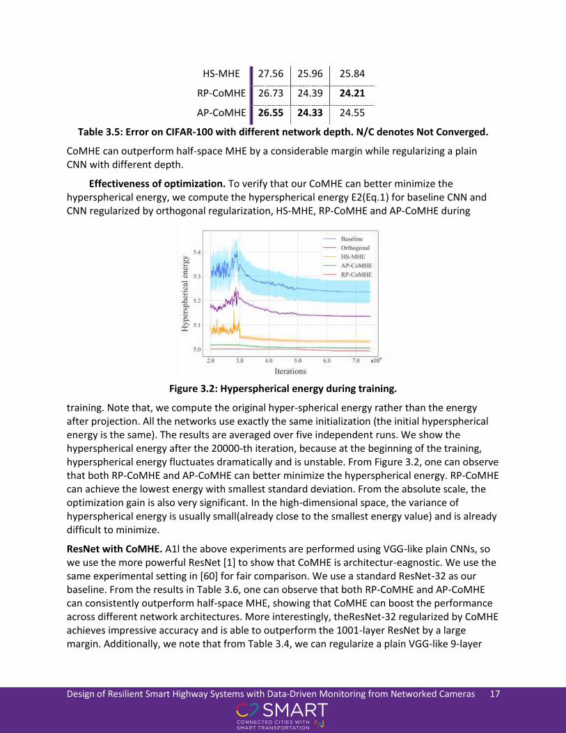
HS-MHE 27.56 25.96 25.84
RP-CoMHE 26.73 24.39 24.21
AP-CoMHE 26.55 24.33 24.55
Table 3.5: Error on CIFAR-100 with different network depth. N/C denotes Not Converged.
CoMHE can outperform half-space MHE by a considerable margin while regularizing a plain CNN with different depth.
Effectiveness of optimization. To verify that our CoMHE can better minimize the hyperspherical energy, we compute the hyperspherical energy E2(Eq.1) for baseline CNN and CNN regularized by orthogonal regularization, HS-MHE, RP-CoMHE and AP-CoMHE during
Figure 3.2: Hyperspherical energy during training.
training. Note that, we compute the original hyper-spherical energy rather than the energy after projection. All the networks use exactly the same initialization (the initial hyperspherical energy is the same). The results are averaged over five independent runs. We show the hyperspherical energy after the 20000-th iteration, because at the beginning of the training, hyperspherical energy fluctuates dramatically and is unstable. From Figure 3.2, one can observe that both RP-CoMHE and AP-CoMHE can better minimize the hyperspherical energy. RP-CoMHE can achieve the lowest energy with smallest standard deviation. From the absolute scale, the optimization gain is also very significant. In the high-dimensional space, the variance of hyperspherical energy is usually small(already close to the smallest energy value) and is already difficult to minimize.
ResNet with CoMHE. A1l the above experiments are performed using VGG-like plain CNNs, so we use the more powerful ResNet [1] to show that CoMHE is architectur-eagnostic. We use the same experimental setting in [60] for fair comparison. We use a standard ResNet-32 as our baseline. From the results in Table 3.6, one can observe that both RP-CoMHE and AP-CoMHE can consistently outperform half-space MHE, showing that CoMHE can boost the performance across different network architectures. More interestingly, theResNet-32 regularized by CoMHE achieves impressive accuracy and is able to outperform the 1001-layer ResNet by a large margin. Additionally, we note that from Table 3.4, we can regularize a plain VGG-like 9-layer
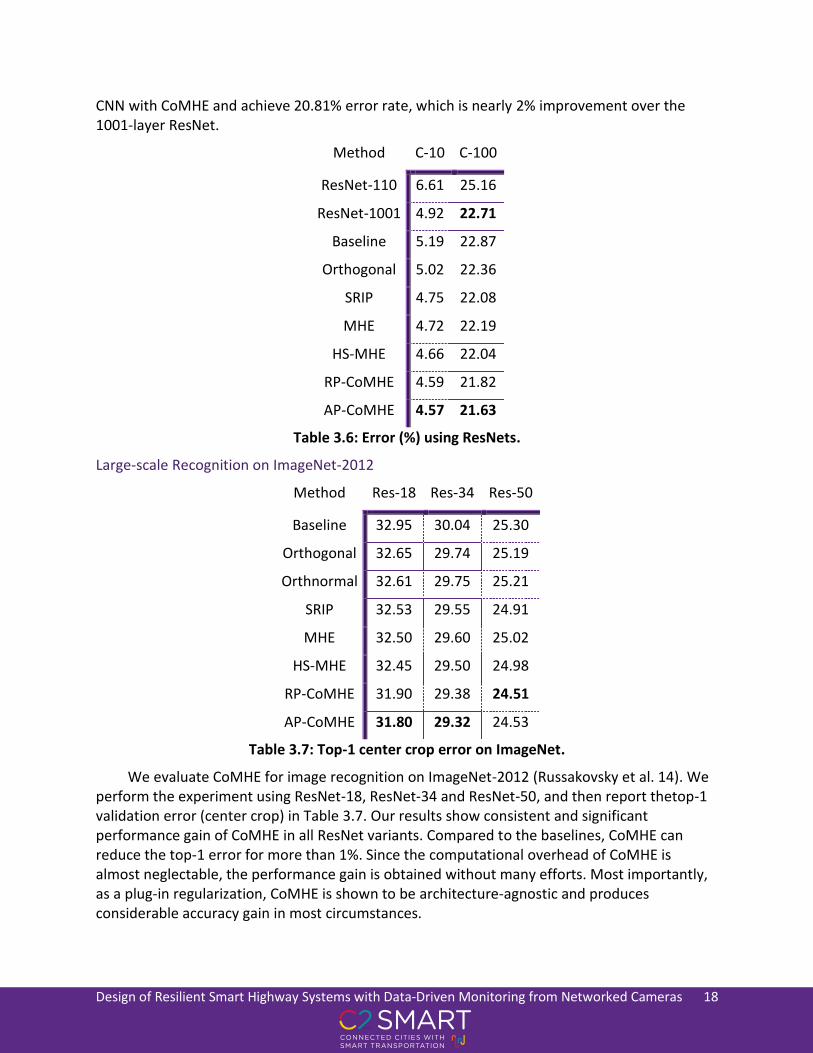
Design of Resilient Smart Highway Systems with Data-Driven Monitoring from Networked Cameras 18
CNN with CoMHE and achieve 20.81% error rate, which is nearly 2% improvement over the 1001-layer ResNet.
Method C-10 C-100
ResNet-110 6.61 25.16
ResNet-1001 4.92 22.71
Baseline 5.19 22.87
Orthogonal 5.02 22.36
SRIP 4.75 22.08
MHE 4.72 22.19
HS-MHE 4.66 22.04
RP-CoMHE 4.59 21.82
AP-CoMHE 4.57 21.63
Table 3.6: Error (%) using ResNets.
Large-scale Recognition on ImageNet-2012
Method Res-18 Res-34 Res-50
Baseline 32.95 30.04 25.30
Orthogonal 32.65 29.74 25.19
Orthnormal 32.61 29.75 25.21
SRIP 32.53 29.55 24.91
MHE 32.50 29.60 25.02
HS-MHE 32.45 29.50 24.98
RP-CoMHE 31.90 29.38 24.51
AP-CoMHE 31.80 29.32 24.53
Table 3.7: Top-1 center crop error on ImageNet.
We evaluate CoMHE for image recognition on ImageNet-2012 (Russakovsky et al. 14). We perform the experiment using ResNet-18, ResNet-34 and ResNet-50, and then report thetop-1 validation error (center crop) in Table 3.7. Our results show consistent and significant performance gain of CoMHE in all ResNet variants. Compared to the baselines, CoMHE can reduce the top-1 error for more than 1%. Since the computational overhead of CoMHE is almost neglectable, the performance gain is obtained without many efforts. Most importantly, as a plug-in regularization, CoMHE is shown to be architecture-agnostic and produces considerable accuracy gain in most circumstances.

Design of Resilient Smart Highway Systems with Data-Driven Monitoring from Networked Cameras 19
Figure 3.3: Visualized first-layer filters.
Besides the accuracy improvement, we also visualize in Figure 3.3 the 64 filters in the first-layer learned by the baseline ResNet and the proposed CoMHE-regularized ResNet. The filters look quite different after we regularize the network using CoMHE. Each filter learned by baseline focuses on a particular local pattern (e.g, edge, color and shape) and each one has a clear local semantic meaning. In contrast, filters learned by CoMHE focuses more on edges, textures and global patterns which do not necessarily have a clear local semantic meaning. However, from a represen-tation basis perspective, having such global patterns may be beneficial to the recognition accuracy. We also observe that filters learned by CoMHE pay less attention to color.
Point Cloud Recognition
We evaluate CoMHE on point cloud recognition. Our goal is to vali-date the effectiveness of CoMHE on a totally different network architecture with a different form of input data structure, rather than achieving state-of-the-art performance on point cloud recognition. To this end, we conduct experiments on widely used neural networks that handles point clouds: Point-Net (PN, Qi et al. 17) and PointNet++ (PN++, Qi et al. 17). We combine half-space MHE, RP-CoMHE and AP-CoMHE into PN(without T-Net), PN(with T-Net) and PN++. We test the performance on ModelNet-40 (Wu et.al 15). Specifically, since PN can be viewed as 1×1 convolutions before the max pooling layer, we can apply all these MHE variants similarly to CNN. After the max pooling layer, there is a standard fully connected network where we can still apply the MHE variants. We compare the performance of regularizing PN and PN++with half-space MHE, RP-COMHE or AP-CoMHE.
Table 3.8 shows that all MHE variants consistently improve PN and PN++, while RP-CoMHE and AP-CoMHE again perform the best among all. We demonstrate that CoMHE is generally useful for different types of input data (not limit to images) and different types of neural networks. CoMHE is also useful in graph neural networks.
Method PN PN (T) PN++
Original 87.1 89.20 90.07
MHE 87.31 89.33 90.25
HS-MHE 87.44 89.41 90.31
RP-CoMHE 87.82 89.69 90.52

Design of Resilient Smart Highway Systems with Data-Driven Monitoring from Networked Cameras 20
AP-CoMHE 87.85 89.70 90.56
Table 3.8: Accuracy (%) on ModelNet-40.
Subsection 3.5 Concluding remarks
Since naively minimizing hyperspherical energy yields suboptimal solutions, we propose a novel framework which projects the neurons to suitable spaces and minimizes the energy there. Experiments validate CoMHE's superiority.

Design of Resilient Smart Highway Systems with Data-Driven Monitoring from Networked Cameras 21
Section 4: Traffic control under faulty sensing Subsection 4.1: Introduction
In this section, we study the traffic routing problem in the presence of unreliable sensing. Feedback dynamic routing is a commonly used control strategy in transportation systems. This class of control strategies relies on real-time information about the traffic state in each link. However, such information may not always be observable due to temporary sensing faults. In this article, we consider dynamic routing over two parallel routes (e.g. in Fig. 4.1), where the sensing on each link is subject to recurrent and random faults. The faults occur and clear according to a finite-state Markov chain. When the sensing is faulty on a link, the traffic state on that link appears to be zero to the controller. Building on the theories of Markov processes and monotone dynamical systems, we derive lower and upper bounds for the resilience score, i.e. the guaranteed throughput of the network, in the face of sensing faults by establishing stability conditions for the network. We use these results to study how a variety of key parameters affect the resilience score of the network. The main conclusions are: (i) Sensing faults can reduce throughput and destabilize a nominally stable network; (ii) A higher failure rate does not necessarily reduce throughput, and there may exist a worst rate that minimizes throughput; (iii) Higher correlation between the failure probabilities of two links leads to greater throughput; (iv) A large difference in capacity between two links can result in a drop in throughput.
Figure 4.1: Selection over parallel routes.
Subsection 4.2: Modeling
Consider the two-link network in Figure 4.2. Let 𝑈𝑘(𝑡) be the flow into link 𝑘 ∈ {1, 2} and 𝑋𝑘(𝑡) be the traffic density of link 𝑘 at time 𝑡. The capacity of link k is 𝐹𝑘 ∈ [0, 1] where 𝐹1 + 𝐹2 =
1. The flow out of link k is 𝑓𝑘(𝑋𝑘(𝑡)), which is specified by the flow function
𝑓𝑘(𝑥𝑘) = 𝐹𝑘(1 − 𝑒−𝑥𝑘 ), 𝑘 = 1, 2.
The source node is subject to a constant demand η ≥ 0, which is considered as a model parameter rather than a state or input variable in the subsequent analysis.
Design of Resilient Smart Highway Systems with Data-Driven Monitoring from Networked Cameras 22
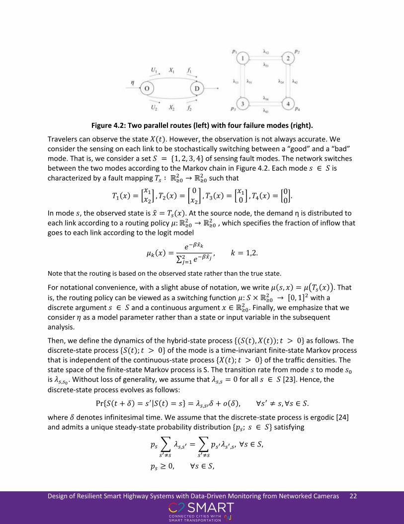
Figure 4.2: Two parallel routes (left) with four failure modes (right).
Travelers can observe the state 𝑋(𝑡). However, the observation is not always accurate. We consider the sensing on each link to be stochastically switching between a “good” and a “bad” mode. That is, we consider a set 𝑆 = {1, 2, 3, 4} of sensing fault modes. The network switches between the two modes according to the Markov chain in Figure 4.2. Each mode 𝑠 ∈ 𝑆 is characterized by a fault mapping 𝑇𝑠 ∶ ℝ≥0
2 → ℝ≥02 such that
𝑇1(𝑥) = [𝑥1
𝑥2] , 𝑇2(𝑥) = [
0𝑥2
] , 𝑇3(𝑥) = [𝑥1
0] , 𝑇4(𝑥) = [
00].
In mode 𝑠, the observed state is �̂� = 𝑇𝑠(𝑥). At the source node, the demand η is distributed to each link according to a routing policy 𝜇:ℝ≥0
2 → ℝ≥02 , which specifies the fraction of inflow that
goes to each link according to the logit model
𝜇𝑘(𝑥) =𝑒−𝛽�̂�𝑘
∑ 𝑒−𝛽�̂�𝑗2𝑗=1
, 𝑘 = 1,2.
Note that the routing is based on the observed state rather than the true state.
For notational convenience, with a slight abuse of notation, we write 𝜇(𝑠, 𝑥) = 𝜇(𝑇𝑠(𝑥)). That
is, the routing policy can be viewed as a switching function 𝜇: 𝑆 × ℝ≥02 → [0, 1]2 with a
discrete argument 𝑠 ∈ 𝑆 and a continuous argument 𝑥 ∈ ℝ≥02 . Finally, we emphasize that we
consider 𝜂 as a model parameter rather than a state or input variable in the subsequent analysis.
Then, we define the dynamics of the hybrid-state process {(𝑆(𝑡), 𝑋(𝑡)); 𝑡 > 0} as follows. The discrete-state process {𝑆(𝑡); 𝑡 > 0} of the mode is a time-invariant finite-state Markov process that is independent of the continuous-state process {𝑋(𝑡); 𝑡 > 0} of the traffic densities. The state space of the finite-state Markov process is S. The transition rate from mode 𝑠 to mode 𝑠0 is 𝜆𝑠,𝑠0
. Without loss of generality, we assume that 𝜆𝑠,𝑠 = 0 for all 𝑠 ∈ 𝑆 [23]. Hence, the
discrete-state process evolves as follows:
Pr{𝑆(𝑡 + 𝛿) = 𝑠′|𝑆(𝑡) = 𝑠} = 𝜆𝑠,𝑠′𝛿 + 𝑜(𝛿), ∀𝑠′ ≠ 𝑠, ∀𝑠 ∈ 𝑆.
where 𝛿 denotes infinitesimal time. We assume that the discrete-state process is ergodic [24] and admits a unique steady-state probability distribution {𝑝𝑠; 𝑠 ∈ 𝑆} satisfying
𝑝𝑠 ∑ 𝜆𝑠,𝑠′ = ∑ 𝑝𝑠′𝜆𝑠′,𝑠,
𝑠′≠𝑠𝑠′≠𝑠
∀𝑠 ∈ 𝑆,
𝑝𝑠 ≥ 0, ∀𝑠 ∈ 𝑆,

Design of Resilient Smart Highway Systems with Data-Driven Monitoring from Networked Cameras 23
∑𝑝𝑠
𝑠∈𝑆
= 1.
The continuous-state process {𝑋(𝑡); 𝑡 > 0} is defined as follows. For any initial condition 𝑆(0) = 𝑠 and 𝑋(0) = 𝑥,
𝑑
𝑑𝑡𝑋𝑘(𝑡) = 𝜂𝜇𝑘(𝑆(𝑡), 𝑋(𝑡)) − 𝑓𝑘(𝑋(𝑡)), 𝑡 ≥ 0, 𝑘 = 1,2.
Note that the routing policy 𝜇 and the flow function 𝑓 ensure that 𝑋(𝑡) is continuous in 𝑡. We
can define the flow dynamics with a vector field 𝐺 ∶ 𝑆 × ℝ≥02 → ℝ2 as follows: 𝐺(𝑠, 𝑥) ≔
𝜂𝜇(𝑠, 𝑥) − 𝑓(𝑥). The joint evolution of 𝑆(𝑡) and 𝑋(𝑡) is in fact a piecewise-deterministic Markov process and can be described compactly using an infinitesimal generator
ℒ𝑔(𝑠, 𝑥) = (𝜂𝜇(𝑠, 𝑥) − 𝑓(𝑥))𝑇∇𝑥𝑔(𝑠, 𝑥) + ∑ 𝜆𝑠,𝑠′(𝑔(𝑠′, 𝑥) − 𝑔(𝑠, 𝑥))
𝑠′∈𝑆
.
for any differentiable function 𝑔.
The network is stable if there exists 𝑍 < ∞ such that for any initial condition (𝑠, 𝑥) ∈ 𝑆 × ℝ≥02
lim sup𝑡→∞
1
𝑡∫ 𝐸[|𝑋(𝑟)|]𝑑𝑟 ≤ 𝑍.
𝑡
𝑟=0
This notion of stability follows a classical definition [25], some authors name it as “first-moment stable” [26]. The rest of this paper is devoted to establishing and analyzing the relation between the stability of the continuous-state process {𝑋(𝑡); 𝑡 > 0} and the demand η.
Subsection 4.2: Analysis
The main result of this section is as follows.
Theorem 1. Consider two parallel links with sensors switching between two modes as defined in section 4.1.
i) A necessary condition for stability is that
𝜂 (1
𝑒−𝛽𝑥2 + 1𝑝2 +
1
2𝑝4) ≤ 𝐹1,
𝜂 (1
𝑒−𝛽𝑥1 + 1𝑝3 +
1
2𝑝4) ≤ 𝐹1,
𝜂 < 1.
where 𝑥𝑘 is the solution to
𝜂𝑒−𝛽𝑥𝑘
1 + 𝑒−𝛽𝑥𝑘= 𝐹𝑘(1 − 𝑒−𝑥𝑘)
for 𝑘 = 1, 2.
ii) A sufficient condition for stability is that there exists 𝜃 ∈ ℝ≥02 such that

Design of Resilient Smart Highway Systems with Data-Driven Monitoring from Networked Cameras 24
∑𝑝𝑠 max𝑘∈{1,2}
{𝜂𝑒−𝛽𝑇𝑠,𝑘(𝜃𝑘)
𝑒−𝛽𝑇𝑠,𝑘(𝜃2) + 𝑒−𝛽𝑇𝑠,𝑘(𝜃1)− 𝐹𝑘(1 − 𝑒−𝜃𝑘)} < 0
4
𝑠=1
.
The rest of this subsection is devoted to the proof of the above result.
Proof of sufficiency:
An apparent necessary condition for stability is 𝜂 < 1. If this does not hold, then the network is unstable even in the absence of sensing faults [27]. First, an invariant set of the process {𝑋(𝑡); 𝑡 > 0} is 𝑀 = [𝑥1 , ∞) × [𝑥2 , ∞). To see this, note that for any 𝑠 ∈ 𝑆 and for any (𝑥1, 𝑥2) ∈ 𝑀𝑐, the vector 𝐺 of time derivatives of the traffic densities has a non-zero component that points to the interior of the invariant set 𝑀; see Figure 4.3.
Figure 4.3: Illustration of the continuous state process and the invariant set 𝑴. The arrows represent the vector field 𝑮 defined in (7) for the four states.
Second, by ergodicity of the process {(𝑆(𝑡), 𝑋(𝑡)); 𝑡 > 0}, we have for 𝑘 ∈ {1, 2},
𝑋𝑘(𝑡) = 𝑋𝑘(0) = ∫ (𝑢𝑘(𝜏) − 𝑓𝑘(𝜏))𝑑𝜏𝑡
𝜏=0
,
where 𝑢𝑘(𝜏) and 𝑓𝑘(𝜏) are inflow and outflow of link k at time 𝜏. Since lim𝑡→∞
1
𝑡𝑋𝑘(0) = 0 and
lim𝑡→∞
1
𝑡𝑋𝑘(𝑡) = 0 a.s., then
0 = lim𝑡→∞
1
𝑡(∫ (𝑢𝑘(𝜏) − 𝑓𝑘(𝜏))𝑑𝜏
𝑡
0
+ 𝑋𝑘(0) − 𝑋𝑘(𝑡)) = lim𝑡→∞
1
𝑡∫ (𝑢𝑘(𝜏) − 𝑓𝑘(𝜏))𝑑𝜏
𝑡
0
𝑎. 𝑠.
Note that 𝑓𝑘(𝜏) ≤ 𝐹𝑘 for any 𝜏 ≥ 0 and 𝑘 ∈ {1, 2}, hence
lim𝑡→∞
1
𝑡∫ 𝑢𝑘(𝜏)𝑑𝜏
𝑡
0
= lim𝑡→∞
1
𝑡∫ 𝑓𝑘(𝜏)𝑑𝜏
𝑡
0
≤ lim𝑡→∞
1
𝑡∫ 𝐹𝑘𝑑𝜏
𝑡
0
= 𝐹𝑘.
According to the definition of steady-state probability,
lim𝑡→∞
1
𝑡∫ 𝕀𝑆(𝜏)=𝑠𝑑𝜏
𝑡
0
= 𝑝𝑠, 𝑎. 𝑠. ∀𝑠 ∈ 𝑆.
Combining with (12), we obtain
Design of Resilient Smart Highway Systems with Data-Driven Monitoring from Networked Cameras 25
𝐹1 ≥ lim𝑡→∞
1
𝑡∫ 𝑢1(𝜏)𝑑𝜏
𝑡
0
= lim𝑡→∞
1
𝑡∫ 𝜂𝜇1(𝑆(𝜏), 𝑋(𝜏))𝑑𝜏
𝑡
0
= 𝜂 lim𝑡→∞
1
𝑡∑∫ 𝕀𝑆(𝜏)=𝑠𝜇1(𝑆(𝜏), 𝑋(𝜏))𝑑𝜏
𝑡
0
4
𝑠=1
≥ 𝜂 lim𝑡→∞
1
𝑡(∫ 𝕀𝑆(𝜏)=10𝑑𝜏
𝑡
0
+ ∫ 𝕀𝑆(𝜏)=2
1
1 + 𝑒−𝛽𝑥2 𝑑𝜏
𝑡
0
+ ∫ 𝕀𝑆(𝜏)=30𝑑𝜏𝑡
0
+ ∫ 𝕀𝑆(𝜏)=4
1
2𝑑𝜏
𝑡
0
) = 𝜂 (1
1 + 𝑒−𝛽𝑥2∫ 𝕀𝑆(𝜏)=2𝑑𝜏
𝑡
0
+1
2lim𝑡→∞
1
𝑡∫ 𝕀𝑆(𝜏)=4𝑑𝜏
𝑡
0
)
= 𝜂 (𝑝2
1 + 𝑒−𝛽𝑥2+
𝑝4
2),
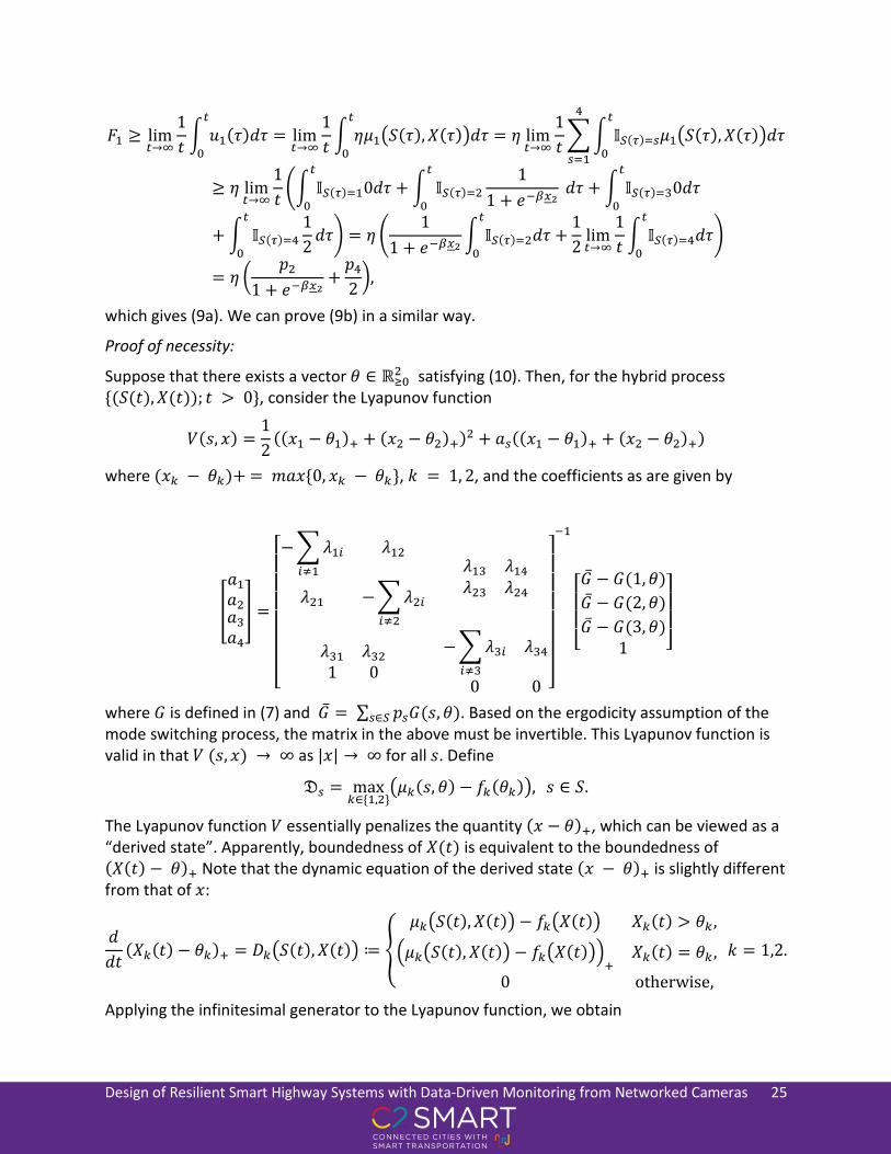
which gives (9a). We can prove (9b) in a similar way.
Proof of necessity:
Suppose that there exists a vector 𝜃 ∈ ℝ≥02 satisfying (10). Then, for the hybrid process
{(𝑆(𝑡), 𝑋(𝑡)); 𝑡 > 0}, consider the Lyapunov function
𝑉(𝑠, 𝑥) =1
2((𝑥1 − 𝜃1)+ + (𝑥2 − 𝜃2)+)2 + 𝑎𝑠((𝑥1 − 𝜃1)+ + (𝑥2 − 𝜃2)+)
where (𝑥𝑘 − 𝜃𝑘)+ = 𝑚𝑎𝑥{0, 𝑥𝑘 − 𝜃𝑘}, 𝑘 = 1, 2, and the coefficients as are given by
[
𝑎1
𝑎2𝑎3
𝑎4
] =
[ − ∑𝜆1𝑖
𝑖≠1
𝜆12
𝜆21 −∑𝜆2𝑖
𝑖≠2
𝜆13 𝜆14
𝜆23 𝜆24
𝜆31 𝜆32
1 0
−∑𝜆3𝑖
𝑖≠3
𝜆34
0 0 ] −1
[ �̅� − 𝐺(1, 𝜃)
�̅� − 𝐺(2, 𝜃)
�̅� − 𝐺(3, 𝜃)1 ]
where 𝐺 is defined in (7) and �̅� = ∑ 𝑝𝑠𝐺(𝑠, 𝜃)𝑠∈𝑆 . Based on the ergodicity assumption of the mode switching process, the matrix in the above must be invertible. This Lyapunov function is valid in that 𝑉 (𝑠, 𝑥) → ∞ as |𝑥| → ∞ for all 𝑠. Define
𝔇𝑠 = max𝑘∈{1,2}
(𝜇𝑘(𝑠, 𝜃) − 𝑓𝑘(𝜃𝑘)), 𝑠 ∈ 𝑆.
The Lyapunov function 𝑉 essentially penalizes the quantity (𝑥 − 𝜃)+, which can be viewed as a “derived state”. Apparently, boundedness of 𝑋(𝑡) is equivalent to the boundedness of (𝑋(𝑡) − 𝜃)+ Note that the dynamic equation of the derived state (𝑥 − 𝜃)+ is slightly different from that of 𝑥:
𝑑
𝑑𝑡(𝑋𝑘(𝑡) − 𝜃𝑘)+ = 𝐷𝑘(𝑆(𝑡), 𝑋(𝑡)) ≔ {
𝜇𝑘(𝑆(𝑡), 𝑋(𝑡)) − 𝑓𝑘(𝑋(𝑡)) 𝑋𝑘(𝑡) > 𝜃𝑘 ,
(𝜇𝑘(𝑆(𝑡), 𝑋(𝑡)) − 𝑓𝑘(𝑋(𝑡)))+
𝑋𝑘(𝑡) = 𝜃𝑘 ,
0 otherwise,
𝑘 = 1,2.
Applying the infinitesimal generator to the Lyapunov function, we obtain
Design of Resilient Smart Highway Systems with Data-Driven Monitoring from Networked Cameras 26
ℒ𝑉(𝑠, 𝑥) = ∑ ∑𝐷𝑗(𝑠, 𝑥)(𝑥𝑘 − 𝜃𝑘)+
2
𝑗=1
2
𝑘=1
+ ∑ (𝜆𝑠,𝑠′(𝑎𝑠′ − 𝑎𝑠) ∑(𝑥𝑘 − 𝜃𝑘)+
2
𝑘=1
) + ∑ 𝑎𝑠,𝑘𝐷𝑘(𝑠, 𝑥)
2
𝑘=1𝑠′≠𝑠
= (∑ 𝐷𝑘
2
𝑘=1
(𝑠, 𝑥) + ∑ 𝜆𝑠,𝑠′(𝑎𝑠′ − 𝑎𝑠)
𝑠′≠𝑠
) |(𝑥𝑘 − 𝜃𝑘)+| + ∑ 𝑎𝑠,𝑘𝐷𝑘(𝑠, 𝑥)
2
𝑘=1
.
This proof establishes the stability of the process {(𝑆(𝑡), 𝑋(𝑡)); 𝑡 > 0} by verifying that the Lyapunov function 𝑉 as defined above satisfies the Foster-Lyapunov drift condition for stability
ℒ𝑉(𝑠, 𝑥) ≤ −𝑐|𝑥| + 𝑑 ∀(𝑠, 𝑥) ∈ 𝑆 × ℝ≥02
for some 𝑐 > 0 and 𝑑 < ∞, where |𝑥| is the one-norm of 𝑥; this condition will imply (8). To proceed, we partition ℝ≥0
2 , the space of 𝑥, into two subsets:
𝒳0 = {𝑥: 0 ≤ 𝑥 ≤ 𝜃},𝒳1 = 𝒳0𝐶;
that is, 𝑋0 and 𝑋1 are the complement to each other in the space ℝ≥02 . In the rest of this proof,
we first verify (16) over 𝑋0 and then over 𝑋1. To verify (16) over 𝑋0, note that 𝜇 and 𝑓 are bounded functions, so, for any 𝑎𝑠,𝑘, there exists 𝑑 < ∞ such that
𝑑1 ≥ 𝑎𝑠 ∑ 𝐷𝑘(𝑠, 𝑥)
2
𝑘=1
∀(𝑠, 𝑥) ∈ 𝑆 × ℝ≥02 .
In addition, (𝑥𝑘 − 𝜃𝑘)+ = 0, 𝑘 = 1, 2, . . . , 𝐾 for all 𝑥 ∈ 𝑋0; this and (15) imply ℒ𝑉(𝑠, 𝑥) ≤𝑑1. Furthermore, for any 𝑐 > 0, there exists 𝑑2 = 𝑐|𝜃| such that 𝑑2 ≥ 𝑐|𝑥| for all 𝑥 ∈ 𝑋0. Hence, letting 𝑑 = 𝑑1 + 𝑑2, we have
ℒ𝑉(𝑠, 𝑥) ≤ −𝑐|𝑥| + 𝑑 ∀(𝑠, 𝑥) ∈ 𝑆 × 𝒳0.
To verify (16) over 𝑋1, we further decompose 𝑋1 into the following subsets:
𝒳11 = {𝑥 ∈ 𝒳1: 𝑥1 ≥ 𝜃1, 𝑥2 < 𝜃2},
𝒳12 = {𝑥 ∈ 𝒳1: 𝑥1 < 𝜃1, 𝑥2 ≥ 𝜃2},
𝒳13 = {𝑥 ∈ 𝒳1: 𝑥1 ≥ 𝜃1, 𝑥2 ≥ 𝜃2}.
For each 𝑥 ∈ 𝑋11, we have
ℒ𝑉(𝑠, 𝑥) = (𝐷1(𝑠, 𝑥) + ∑ 𝜆𝑠,𝑠′(𝑎𝑠′ − 𝑎𝑠)
𝑠′≠𝑠
) |(𝑥 − 𝜃)+| + 𝑎𝑠 ∑ 𝐷𝑘(𝑠, 𝑥)
2
𝑘=1
≤ ((𝜇1(𝑠, 𝑥) − 𝑓1(𝑥1)) + ∑ 𝜆𝑠,𝑠′(𝑎𝑠′ − 𝑎𝑠)
𝑠′≠𝑠
) |(𝑥 − 𝜃)+| + 𝑑1
≤ (𝔇𝑠 + ∑ 𝜆𝑠,𝑠′(𝑎𝑠′ − 𝑎𝑠)
𝑠′≠𝑠
) |(𝑥 − 𝜃)+| + 𝑑1.

Design of Resilient Smart Highway Systems with Data-Driven Monitoring from Networked Cameras 27
From the definition of 𝑎𝑠, we have
𝔇𝑠 + ∑ 𝜆𝑠,𝑠′(𝑎𝑠′ − 𝑎𝑠)
𝑠′≠𝑠
=1
4∑ 𝑝𝑠′𝔇𝑠′
𝑠′∈𝑆
.
The above and (20) imply
ℒ𝑉(𝑠, 𝑥) ≤1
4(∑ 𝑝𝑠′𝔇𝑠′𝑠′∈𝑆 . )|𝑥| + 𝑑, 𝑥 ∈ 𝒳1
1.
Let 𝑐 ≔ −1
4∑ 𝑝𝑠′𝐷𝑠′𝑠′∈𝑆 . Hence, we have
ℒ𝑉(𝑠, 𝑥) ≤ −𝑐|𝑥| + 𝑑 ∀(𝑠, 𝑥) ∈ 𝑆 × 𝒳11.
Analogously, we can show
ℒ𝑉(𝑠, 𝑥) ≤ −𝑐|𝑥| + 𝑑 ∀(𝑠, 𝑥) ∈ 𝑆 × (𝒳12 ∪ 𝒳1
3),
which completes the proof.
Subsection 4.3: Results
In this section, we study the resilience score, i.e. the guaranteed throughput (the supremum of η that maintains stability), under various scenarios. We first consider two symmetric links and focus on the impact of transition rates of the discrete state. Then, we study how the throughput varies with the asymmetry of the links.
If the two links are homogeneous in the sense that they have same flow functions 𝑓1 = 𝑓2, we have the main result of this section as follows:
Proposition 1. For the homogeneous network, the resilience score 𝜂∗ , i.e. the guaranteed throughput has a lower bound of
𝜂∗ ≥1
1 + 𝑝2 + 𝑝3.
Next, we discuss how characteristics of link failures (specifically, link failure rate and link failure correlation) affect the resilience score. Table 4.1 lists the nominal values considered in this subsection.
Parameter Notation Nominal value
Link 1 capacity 𝐹1 0.5
Link 2 capacity 𝐹2 0.5
Routing sensitivity to congestion
𝛽 1
Table 4.1: Nominal model parameters
Link failure rate: Suppose that the health of each link is independent of the other link. Furthermore, suppose that the failure rates of both links are identical, denoted as 𝑝, then

Design of Resilient Smart Highway Systems with Data-Driven Monitoring from Networked Cameras 28
𝑝2 + 𝑝4 = 𝑝 = 𝑝3 + 𝑝4,
𝜂∗ =1
1 + 𝑝2 + 𝑝3=
1
1 + 2𝑝(1 − 𝑝).
When the link failure rate is either 0 or 1, the two-link network becomes open-loop, the lower bound can naturally be 1. The lower bound reaches minimum when the link failure rate is 0.5; see Figure 4.4.
Figure 4.4: Impact of link failure probability (𝝆 = 𝟎) and link failure correlation (𝒑 = 𝟎. 𝟓) on the lower bound of resilience score.
Link failure correlation: Suppose that the health of each link is correlated with the other link while the failure rates of both links are still identical. Denote the correlation as 𝜌, then
𝜌 =𝑝4 − (𝑝2 + 𝑝4)(𝑝3 + 𝑝4)
√𝑝2𝑝3
=𝑝 − 𝑝2 − 𝑝2
𝑝,
𝜂∗ =1
1 + 𝑝2 + 𝑝3=
1
1 + 2𝑝(1 − 𝑝 − 𝜌).
As the link failure correlation increases from −𝑝 to 1 − 𝑝, the lower bound increases from 1
1+2𝑝 to 1. When the failure of the two links are strongly (positively) correlated, the two-link
network also turns to be open-loop and hence the lower bound reaches 1; see Figure 4.4.
Now we relax the assumption of symmetric links and allow 𝐹1 ≠ 𝐹2. Without loss of generality, we assume that 𝐹1 ≥ 𝐹2. Instead, we will consider symmetric failure rate, i.e. 𝑝2 = 𝑝3. The following result links the resilience score to |𝐹1 − 𝐹2|, which quantifies the asymmetry of links:
Proposition 2. Suppose that 𝑝2 = 𝑝3 and 𝐹1 ≥ 𝐹2. Then, the resilience score has a lower bound of
𝜂∗ ≥ min {1 − (𝐹1 − 𝐹2)
1 − 𝑝1,1 − 𝑝4(𝐹1 − 𝐹2)
1 + 2𝑝2}.
The proofs of Propositions 1 and 2 are available in (Xie & Jin 2020).
Now we are ready to discuss how link capacity difference affects the resilience score. When
𝐹1 = 𝐹2, the lower bound is 1
1+2𝑝2 , in consistence with our lower bound in subsection 4.1, and
the upper bound is 1 (note that when √2 𝑚𝑎𝑥{𝑝2, 𝑝3} + 𝑝4 ≤ 1, we can derive 𝜂 < 1 from the necessary condition).
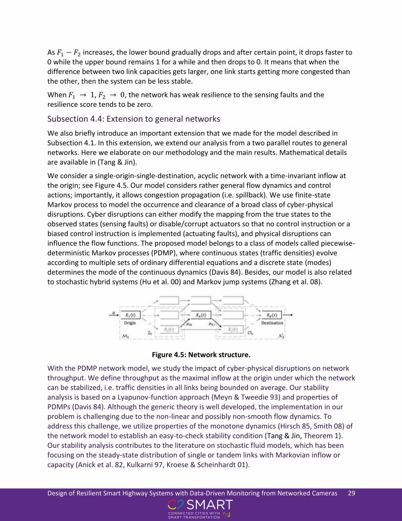
Design of Resilient Smart Highway Systems with Data-Driven Monitoring from Networked Cameras 29
As 𝐹1 − 𝐹2 increases, the lower bound gradually drops and after certain point, it drops faster to 0 while the upper bound remains 1 for a while and then drops to 0. It means that when the difference between two link capacities gets larger, one link starts getting more congested than the other, then the system can be less stable.
When 𝐹1 → 1, 𝐹2 → 0, the network has weak resilience to the sensing faults and the resilience score tends to be zero.
Subsection 4.4: Extension to general networks
We also briefly introduce an important extension that we made for the model described in Subsection 4.1. In this extension, we extend our analysis from a two parallel routes to general networks. Here we elaborate on our methodology and the main results. Mathematical details are available in (Tang & Jin).
We consider a single-origin-single-destination, acyclic network with a time-invariant inflow at the origin; see Figure 4.5. Our model considers rather general flow dynamics and control actions; importantly, it allows congestion propagation (i.e. spillback). We use finite-state Markov process to model the occurrence and clearance of a broad class of cyber-physical disruptions. Cyber disruptions can either modify the mapping from the true states to the observed states (sensing faults) or disable/corrupt actuators so that no control instruction or a biased control instruction is implemented (actuating faults), and physical disruptions can influence the flow functions. The proposed model belongs to a class of models called piecewise-deterministic Markov processes (PDMP), where continuous states (traffic densities) evolve according to multiple sets of ordinary differential equations and a discrete state (modes) determines the mode of the continuous dynamics (Davis 84). Besides, our model is also related to stochastic hybrid systems (Hu et al. 00) and Markov jump systems (Zhang et al. 08).
Figure 4.5: Network structure.
With the PDMP network model, we study the impact of cyber-physical disruptions on network throughput. We define throughput as the maximal inflow at the origin under which the network can be stabilized, i.e. traffic densities in all links being bounded on average. Our stability analysis is based on a Lyapunov-function approach (Meyn & Tweedie 93) and properties of PDMPs (Davis 84). Although the generic theory is well developed, the implementation in our problem is challenging due to the non-linear and possibly non-smooth flow dynamics. To address this challenge, we utilize properties of the monotone dynamics (Hirsch 85, Smith 08) of the network model to establish an easy-to-check stability condition (Tang & Jin, Theorem 1). Our stability analysis contributes to the literature on stochastic fluid models, which has been focusing on the steady-state distribution of single or tandem links with Markovian inflow or capacity (Anick et al. 82, Kulkarni 97, Kroese & Scheinhardt 01).

Design of Resilient Smart Highway Systems with Data-Driven Monitoring from Networked Cameras 30
Next, we propose control design based on the stability analysis. In practice, a key challenge for resilient control is that one cannot always have a full observation of network states and disruption modes. We focus on three typical cases. In the first case, the network links may have finite storage spaces, and the system operator can observe disruption modes. For this case, we show that there must exist a mode-dependent control that will attain the expected-min-cut capacity of the network (Tang & Jin, Theorem 2). In the second case, all of the network links have infinite storage space, and the system operator has no observation but perfect knowledge of disruptions. For this case, we propose an open-loop control that attains the min-expected-cut capacity of the network (Tang & Jin, Theorem 3). These results are analogous to the classical max-flow min-cut theorem (Dantzig & Fulkersen 03). In the third case, the system observer can only observe traffic densities. We propose a density-dependent control that mitigates congestion spillback and provide a lower bound for the guaranteed throughput (Tang & Jin, Theorem 4). Finally, we use numerical examples to demonstrate that our control design approach can enhance the network resiliency.
Subsection 4.5: Subsequent work: Simulation of I210
As a follow-up work of this project, we will validate our results on I210. We have created a simulation testbed for traffic flow on Interstate I210 near Los Angeles. This model will be used for simulating sensing faults and the impact of feedback ramp control.
Figure 4.6: Simulation testbed for I210 near Los Angeles.

Design of Resilient Smart Highway Systems with Data-Driven Monitoring from Networked Cameras 31
Section 5: Conclusions In this project, we considered the traffic monitoring and control problem in the presence of unstable sensing. We explored ideas from computer vision and traffic control, which provides a basis for subsequent implementation.
For traffic control, we propose a two-link dynamic flow model with sensing faults to study the stability conditions and guaranteed throughput of the network. Based on this model, we are able to derive lower and upper bounds of the resilience score and analyze the impact of transition rates and heterogeneous link capacities on them. This work can be extended in several directions. First, we can consider a complicated network with k links (not necessarily parallel) rather than a simple two parallel link network. Second, other forms of flow functions can be assumed in the model. Third, the logit model can be replaced with other routing polices. Last, several variations of fault modes can also be discussed.

Design of Resilient Smart Highway Systems with Data-Driven Monitoring from Networked Cameras 32
References Traffic control
1. David Anick, Debasis Mitra, and Man Mohan Sondhi. Stochastic theory of a datahandling system with multiple sources. The Bell System Technical Journal, 61(8):1871– 1894, 1982.
2. M. Blanke, M. Kinnaert, J. Lunze, M. Staroswiecki, and J. Schr¨oder, Diagnosis and fault-tolerant control. Springer, 2006, vol. 2.
3. G. Como, K. Savla, D. Acemoglu, M. A. Dahleh, and E. Frazzoli, “Robust distributed routing in dynamical networkspart i: Locally responsive policies and weak resilience,” IEEE Transactions on Automatic Control, vol. 58, no. 2, pp. 317–332, 2012.
4. S. Coogan and M. Arcak, “A compartmental model for traffic networks and its dynamical behavior,” IEEE Transactions on Automatic Control, vol. 60, no. 10, pp. 2698–2703, 2015.
5. Mark H A Davis. Piecewise-deterministic Markov processes: A general class of nondiffusion stochastic models. Journal of the Royal Statistical Society. Series B. Methodological, 46(3):353–388, 1984.
6. G Dantzig and Delbert Ray Fulkerson. On the max flow min cut theorem of networks. Linear inequalities and related systems, 38:225–231, 2003.
7. G. Gomes and R. Horowitz, “Optimal freeway ramp metering using the asymmetric cell transmission model,” Transportation Research Part C: Emerging Technologies, vol. 14, no. 4, pp. 244–262, 2006.
8. Morris W Hirsch. Systems of differential equations that are competitive or cooperative ii: Convergence almost everywhere. SIAM Journal on Mathematical Analysis, 16(3):423– 439, 1985.
9. Jianghai Hu, John Lygeros, and Shankar Sastry. Towards a theory of stochastic hybrid systems. In International Workshop on Hybrid Systems: Computation and Control, pages 160–173. Springer, 2000
10. Dirk P Kroese and Werner RW Scheinhardt. Joint distributions for interacting fluid queues. Queueing systems, 37(1-3):99–139, 2001.
11. Vidyadhar G Kulkarni. Fluid models for single buffer systems. Frontiers in queueing: Models and applications in science and engineering, 321:338, 1997.
12. G. Como, K. Savla, D. Acemoglu, M. A. Dahleh, and E. Frazzoli, “Robust distributed routing in dynamical networkspart i: Locally responsive policies and weak resilience,” IEEE Transactions on Automatic Control, vol. 58, no. 2, pp. 317–332, 2012.
13. Sean P Meyn and Richard L Tweedie. Stability of Markovian processes III: FosterLyapunov criteria for continuous-time processes. Advances in Applied Probability, pages 518–548, 1993.
Design of Resilient Smart Highway Systems with Data-Driven Monitoring from Networked Cameras 33
14. P. Mhaskar, A. Gani, N. H. El-Farra, C. McFall, P. D. Christofides, and J. F. Davis, “Integrated fault-detection and fault-tolerant control of process systems,” AIChE Journal, vol. 52, no. 6, pp. 2129–2148, 2006.
15. R. J. Patton, “Fault-tolerant control: the 1997 situation,” IFAC Proceedings Volumes, vol. 30, no. 18, pp. 1029–1051, 1997.
16. J. Reilly, S. Samaranayake, M. L. Delle Monache, W. Krichene, P. Goatin, and A. M. Bayen, “Adjoint-based optimization on a network of discretized scalar conservation laws with applications to coordinated ramp metering,” Journal of optimization theory and applications, vol. 167, no. 2, pp. 733–760, 2015.
17. Hal L Smith. Monotone Dynamical Systems: An Introduction to the Theory of Competitive and Cooperative Systems, volume 41. American Mathematical Soc., 2008.
18. Tang, Y. and Jin, L. Analysis and control of dynamic flow networks subject to stochastic cyber-physical disruptions. Automatica. Under review.
19. X. Tang, G. Tao, and S. M. Joshi, “Adaptive actuator failure compensation for nonlinear mimo systems with an aircraft control application,” Automatica, vol. 43, no. 11, pp. 1869–1883, 2007.
20. Xie, Q. and Jin, L. 2020. Resilience of Dynamic Routing in the Face of Recurrent and Random Sensing Faults. In 2020 American Control Conference.
21. H. Yu and M. Krstic, “Traffic congestion control for aw–rascle–zhang model,” Automatica, vol. 100, pp. 38–51, 2019.
22. Lixian Zhang, El-Kebir Boukas, and James Lam. Analysis and synthesis of markov jump linear systems with time-varying delays and partially known transition probabilities. IEEE Transactions on Automatic Control, 53(10):2458–2464, 2008.
23. Y. Zhang and J. Jiang, “Bibliographical review on reconfigurable fault-tolerant control systems,” Annual reviews in control, vol. 32, no. 2, pp. 229–252, 2008.
24. X. Zhang, T. Parisini, and M. M. Polycarpou, “Adaptive fault-tolerant control of nonlinear uncertain systems: an information-based diagnostic approach,” IEEE Transactions on automatic Control, vol. 49, no. 8, pp. 1259–1274, 2004.
Computer vision
1. Kaiming He, Xiangyu Zhang, Shaoqing Ren, and Jian Sun. Deep residual learning for image recognition. In CVPR, 2016. 1, 6, 8, 12
2. Ross Girshick, Jeff Donahue, Trevor Darrell, and Jitendra Malik. Rich feature hierarchies for accurate object detection and semantic segmentation. In CVPR, 2014. 1
3. Jonathan Long, Evan Shelhamer, and Trevor Darrell. Fully convolutional networks for semantic segmentation. In CVPR, 2015. 1
4. Sergey Ioffe and Christian Szegedy. Batch normalization: Accelerating deep network training by reducing internal co- variate shift. In ICML, 2015. 1, 6
Design of Resilient Smart Highway Systems with Data-Driven Monitoring from Networked Cameras 34
5. Nitish Srivastava, Geoffrey Hinton, Alex Krizhevsky, Ilya Sutskever, and Ruslan Salakhutdinov. Dropout: A simple way to prevent neural networks from overfitting. JMLR, 15(1):1929–1958, 2014. 1
6. Tim Salimans and Diederik P Kingma. Weight normalization: A simple reparameterization to accelerate training of deep neural networks. In NIPS, 2016. 1
7. Andrew M Saxe, James L McClelland, and Surya Ganguli. Exact solutions to the nonlinear dynamics of learning in deep linear neural networks. arXiv preprint arXiv:1312.6120, 2013. 1
8. Dmytro Mishkin and Jiri Matas. All you need is a good init. In ICLR, 2016. 1, 3 9. Nitin Bansal, Xiaohan Chen, and Zhangyang Wang. Can we gain more from orthogonality
regularizations in training deep networks? In NeurIPS, 2018. 1, 3, 6, 8 10. [Pau Rodr´ıguez, Jordi Gonzalez, Guillem Cucurull, Josep M Gonfaus, and Xavier
Roca. Regularizing cnns with locally constrained decorrelations. arXiv preprint arXiv:1611.01967, 2016. 1
11. Lei Huang, Xianglong Liu, Bo Lang, Adams Wei Yu, Yongliang Wang, and Bo Li. Orthogonal weight normaliza- tion: Solution to optimization over multiple dependent stiefel manifolds in deep neural networks. In AAAI, 2018. 1
12. Weiyang Liu, Rongmei Lin, Zhen Liu, Lixin Liu, Zhiding Yu, Bo Dai, and Le Song. Learning towards minimum hyperspherical energy. NeurIPS, 2018. 1, 2, 3, 6, 7, 8, 12, 13, 15, 25
13. J Batle, Armen Bagdasaryan, M AbdelAty, S Abdalla. Generalized thomson problem in arbitrary dimensions and non-euclidean geometries. Physical A: Statistical Mechanics and its Applications, 451:237–250, 2016. 2
14. Matthew Calef, Whitney Griffiths, and Alexia Schulz. Estimating the number of stable configurations for the generalized thomson problem. Journal of Statistical Physics, 160(1):239–253, 2015. 2
15. Y Xiang, DY Sun, W Fan, and XG Gong. Generalized simulated annealing algorithm and its application to the thomson model. Physics Letters A, 233(3):216–220, 1997. 2
16. Y Xiang, XG Gong. Efficiency of generalized simulated annealing. Physical Review E, 62(3):4473, 2000. 2
17. Kenji Kawaguchi, Bo Xie, and Le Song. Deep semi-random features for nonlinear function approximation. In AAAI, 2018. 2, 6
18. Ali Rahimi and Benjamin Recht. Random features for large- scale kernel machines. In NIPS, 2008. 2
19. Zeev Nehari. Conformal mapping. Courier Corporation, 2012. 2 20. Julien Mairal, Francis Bach, Jean Ponce, and Guillermo Sapiro. Online dictionary learning
for sparse coding. In ICML, 2009. 3 21. Ignacio Ramirez, Pablo Sprechmann, and Guillermo Sapiro. Classification and clustering
via dictionary learning with structured incoherence and shared features. In CVPR, 2010. 3
22. Nan Li, Yang Yu, and Zhi-Hua Zhou. Diversity regularized ensemble pruning. In Joint European Conference on Machine Learning and Knowledge Discovery in Databases, 2012. 3
Design of Resilient Smart Highway Systems with Data-Driven Monitoring from Networked Cameras 35
23. Ludmila I Kuncheva and Christopher J Whitaker. Measures of diversity in classifier ensembles and their relationship with the ensemble accuracy. Machine learning, 51(2):181–207, 2003. 3
24. Lu Jiang, Deyu Meng, ShoouI Yu, Zhenzhong Lan, Shiguang Shan, and Alexander Hauptmann. Self-paced learning with diversity. In NIPS, 2014. 3
25. Pengtao Xie, Wei Wu, Yichen Zhu, and Eric P Xing. Orthogonality-promoting distance metric learning: convex relaxation and theoretical analysis. In ICML, 2018. 3
26. Pengtao Xie, Jun Zhu, and Eric Xing. Diversity-promoting bayesian learning of latent variable models. In ICML, 2016. 3
27. Pengtao Xie, Aarti Singh, and Eric P Xing. Uncorrelation and evenness: a new diversity-promoting regularizer. In ICML, 2017. 3
28. Michael Cogswell, Faruk Ahmed, Ross Girshick, Larry Zit- nick, and Dhruv Batra. Reducing overfitting in deep net- works by decorrelating representations. In ICLR, 2016. 3
29. Pau Rodr´ıguez, Jordi Gonzalez, Guillem Cucurull, Josep M Gonfaus, and Xavier Roca. Regularizing cnns with locally constrained decorrelations. In ICLR, 2017. 3, 6, 8
30. Di Xie, Jiang Xiong, Shiliang Pu. All you need is beyond a good init: Exploring better solution for training extremely deep convolutional neural networks with orthonormality and modulation. arXiv:1703.01827, 2017. 3
31. Weiyang Liu, Yandong Wen, Zhiding Yu, and Meng Yang. Large-margin softmax loss for convolutional neural net- works. In ICML, 2016. 3
32. Weiyang Liu, Yan-Ming Zhang, Xingguo Li, Zhiding Yu, Bo Dai, Tuo Zhao, and Le Song. Deep hyperspherical learn- ing. In NIPS, 2017. 3, 6, 8, 12
33. Weiyang Liu, Yandong Wen, Zhiding Yu, Ming Li, Bhiksha Raj, and Le Song. Sphereface: Deep hypersphere embedding for face recognition. In CVPR, 2017. 3
34. Weiyang Liu, Zhen Liu, Zhiding Yu, Bo Dai, Rongmei Lin, Yisen Wang, James M Rehg, and Le Song. Decoupled net- works. CVPR, 2018. 3, 6
35. Jiankang Deng, Jia Guo, and Stefanos Zafeiriou. Arcface: Additive angular margin loss for deep face recognition. arXiv preprint arXiv:1801.07698, 2018. 3
36. Hao Wang, Yitong Wang, Zheng Zhou, Xing Ji, Zhifeng Li, Dihong Gong, Jingchao Zhou, and Wei Liu. Cosface: Large margin cosine loss for deep face recognition. arXiv preprint arXiv:1801.09414, 2018. 3
37. Feng Wang, Xiang Xiang, Jian Cheng, and Alan L Yuille. Normface: L2 hypersphere embedding for face verification. arXiv preprint arXiv:1704.06369, 2017. 3
38. Feng Wang, Weiyang Liu, Haijun Liu, and Jian Cheng. Additive margin softmax for face verification. arXiv preprint arXiv:1801.05599, 2018. 3
39. Weiyang Liu, Zhen Liu, James M Rehg, and Le Song. Neural similarity learning. In NeurIPS, 2019. 3, 6
40. Pascal Mettes, Elise van der Pol, and Cees Snoek. Hyper- spherical prototype networks. In NeurIPS, 2019. 3
41. Harald Crame´r. Mathematical methods of statistics (PMS-9), volume 9. Princeton university press, 2016. 4
42. Chelsea Finn, Pieter Abbeel, and Sergey Levine. Model- agnostic meta-learning for fast adaptation of deep networks. In ICML, 2017. 4

Design of Resilient Smart Highway Systems with Data-Driven Monitoring from Networked Cameras 36
43. Hanxiao Liu, Karen Simonyan, and Yiming Yang. Darts: Differentiable architecture search. arXiv preprint arXiv:1806.09055, 2018. 4
44. Bo Dai, Hanjun Dai, Niao He, Weiyang Liu, Zhen Liu, Jian shu Chen, Lin Xiao, and Le Song. Coupled variational bayes via optimization embedding. In NIPS, 2018. 4
45. Ian Goodfellow, Jean Pouget-Abadie, Mehdi Mirza, Bing Xu, David Warde-Farley, Sherjil Ozair, Aaron Courville, and Yoshua Bengio. Generative adversarial nets. In NIPS, 2014. 4
46. Yuxin Wu and Kaiming He. Group normalization. In ECCV, 2018. 5 47. Sanjoy Dasgupta and Anupam Gupta. An elementary proof of a theorem of johnson and
lindenstrauss. Random Structures & Algorithms, 22(1):60–65, 2003. 5, 17 48. Ata Kaban. Improved bounds on the dot product under random projection and random
sign projection. In KDD, 2015. 5, 17 49. Qinfeng Shi, Chunhua Shen, Rhys Hill, and Anton van den Hengel. Is margin preserved
after random projection? arXiv preprint arXiv:1206.4651, 2012. 5, 18 50. Juan A Cuesta-Albertos, Antonio Cuevas, and Ricardo Fraiman. On projection-based
tests for directional and com- positional data. Statistics and Computing, 19(4):367, 2009. 5
51. Robert J Durrant and Ata Kaba´n. Random projections as regularizers: learning a linear discriminant from fewer observations than dimensions. Machine Learning, 2015. 6
52. Eric P Xing, Michael I Jordan, Stuart J Russell, and An- drew Y Ng. Distance metric learning with application to clustering with side-information. In NIPS, 2003. 6
53. Richard Baraniuk, Mark Davenport, Ronald DeVore, and Michael Wakin. A simple proof of the restricted isometry property for random matrices. Constructive Approximation, 2008. 6
54. Yaniv Plan and Roman Vershynin. One-bit compressed sensing by linear programming. Communications on Pure and Applied Mathematics, 2013. 6
55. Emmanuel J Cande`s, Justin Romberg, and Terence Tao. Ro- bust uncertainty principles: Exact signal reconstruction from highly incomplete frequency information. IEEE Transactions on information theory, 2006. 6
56. Tianyi Zhou and Dacheng Tao. Godec: Randomized low- rank & sparse matrix decomposition in noisy case. In ICML, 2011. 6, 20
57. Nir Ailon and Bernard Chazelle. Approximate nearest neighbors and the fast johnson-lindenstrauss transform. In SOTC, 2006. 6
58. Moses Charikar, Kevin Chen, and Martin Farach-Colton. Finding frequent items in data streams. Theoretical Com- puter Science, 2004. 6
59. Andrew Brock, Theodore Lim, James M Ritchie, and Nick Weston. Neural photo editing with introspective adversarial networks. arXiv preprint arXiv:1609.07093, 2016. 6
60. Kaiming He, Xiangyu Zhang, Shaoqing Ren, and Jian Sun. Identity mappings in deep residual networks. In ECCV, 2016. 8
61. Olga Russakovsky, Jia Deng, Hao Su, Jonathan Krause, Sanjeev Satheesh, Sean Ma, Zhiheng Huang, Andrej Karpathy, Aditya Khosla, Michael Bernstein, et al. Imagenet large scale visual recognition challenge. IJCV, pages 1–42, 2014. 8
62. Charles R Qi, Hao Su, Kaichun Mo, and Leonidas J Guibas. Pointnet: Deep learning on point sets for 3d classification and segmentation. In CVPR, 2017. 8, 13

Design of Resilient Smart Highway Systems with Data-Driven Monitoring from Networked Cameras 37
63. Charles Ruizhongtai Qi, Li Yi, Hao Su, and Leonidas J Guibas. Pointnet++: Deep hierarchical feature learning on point sets in a metric space. In NIPS, 2017. 8, 13
64. Zhirong Wu, Shuran Song, Aditya Khosla, Fisher Yu, Lin- guang Zhang, Xiaoou Tang, and Jianxiong Xiao. 3d shapenets: A deep representation for volumetric shapes. In CVPR, 2015. 8
65. Alex Krizhevsky, Ilya Sutskever, and Geoffrey E Hinton. Imagenet classification with deep convolutional neural net- works. In NIPS, 2012. 12
66. Weiyang Liu, Rongmei Lin, Zhen Liu, James M Rehg, Li Xiong, and Le Song. Orthogonal over-parameterized training. arXiv preprint arXiv:2004.04690, 2020. 14, 21
67. Kaiming He, Xiangyu Zhang, Shaoqing Ren, and Jian Sun. Delving deep into rectifiers: Surpassing human-level perfor- mance on imagenet classification. In ICCV, 2015. 14
68. Juan Antonio Cuesta-Albertos, Ricardo Fraiman, and Thomas Ransford. A sharp form of the cramer–wold the- orem. Journal of Theoretical Probability, 20(2):201–209, 2007. 19
69. Thomas N Kipf and Max Welling. Semi-supervised classi- fication with graph convolutional networks. arXiv preprint arXiv:1609.02907, 2016. 25