Design of Miniaturized Underwater Vehicle with Propulsions … · Design of Miniaturized Underwater...

Design of Miniaturized Underwater Vehicle with

Propulsions for Deep-sea Research Applications

by

Saeed A. Merza

A Thesis Presented in Partial Fulfillment of the Requirements for the Degree

Doctor of Philosophy

Approved June 2014 by the Graduate Supervisory Committee:

Deirdre Ruth Meldrum, Chair

Shih-Hui Chao Praveen Shankar Srikanth Saripalli

Spring Melody Berman

Arizona State University

August 2014

i

ABSTRACT

The ocean is vital to the health of our planet but remains virtually unexplored.

Many researchers seek to understand a wide range of geological and biological

phenomena by developing technologies which enable exploration of the deep-sea. The

task of developing a technology which can withstand extreme pressure and temperature

gradients in the deep ocean is not trivial. Of these technologies, underwater vehicles

were developed to study the deep ocean, but remain large and expensive to manufacture.

I am proposing the development of cost efficient miniaturized underwater vehicle (mUV)

with propulsion systems to carry small measurement devices and enable deep-sea

exploration. These mUV’s overall size is optimized based on the vehicle parameters such

as energy density, desired velocity, swimming time and propulsion performance.

However, there are limitations associated with the size of the mUV which leads to certain

challenges. For example, 2000 m below the sea level, the pressure is as high as 3000 psi.

Therefore, certain underwater vehicle modules, such as the propulsion system, will

require pressure housing to ensure the functionality of the thrust generation. In the case of

a mUV swimming against the deep-sea current, a thrust magnitude is required to enable

the vehicle to overcome the ocean current speed and move forward. Therefore, the size of

the mUV is limited by the energy density and the propeller size. An equation is derived to

miniaturize underwater vehicle while performing with a certain specifications. An

inrunner three-phase permanent magnet brushless DC motor is designed and fabricated

with a specific size to fit inside the mUV’s core. The motor is composed of stator

winding in a pressure housing and an open to water ring-propeller rotor magnet. Several

ring-propellers are 3D printed and tested experimentally to determine their performances

ii

and efficiencies. A planer motion optimal trajectory for the mUV is determined to

minimize the energy usage. Those studies enable the design of size optimized underwater

vehicle with propulsion to carry small measurement sensors and enable underwater

exploration. Developing mUV’s will enable ocean exploration that can lead to significant

scientific discoveries and breakthroughs that will solve current world health and

environmental problems.

iii

ACKNOWLEDGMENTS

As an ordinary high school student form Kurdistan, Iraq with the struggle to have a

peaceful life, I was blessed with the chance to immigrate to the United States of America

in 1999. I could not attend university right away due to financial issues that I faced in my

first year in Phoenix, Arizona. However, if it were not for my family, who gave me the

full support including financial and mortal supports, I would have not had the chance to

start my education in my new country.

At first, I would like to thank all of my brothers and sisters (Ashwaq Ahmad,

Bassam Saeed, Saman Merza and Saineb Ahmad) for their faith in me. I also would like

to thank my friends for their encouragement and their confidence in me.

Most of all, I would like to give my gratitude to my advisors, Dr. Deirdre

Meldrum, Dr. Shih-hui Chao, Dr. Praveen Shankar, Dr. Srikanth Saripalli and Dr. Spring

Melody Berman. They patiently provided the vision, encouragement and advice

necessary for me to proceed through the doctoral program and complete my dissertation.

Their unflagging encouragement and serving is the best role models to me as a junior

member of academia.

Finally, I would like to thank Arizona State University NEPTUNE fund for their

generous support. And all the staff and students at CBDA, I’m grateful to join and be a

part of the lab. Thank you for treating me as a friend and helping me to achieve my

project. Special thanks to my colleagues, Jieying, Bo, Jia for discussion and consolation.

iv

TABLE OF CONTENTS

Page

ABSTRACT ........................................................................................................................ i

ACKNOWLEDGMENTS ................................................................................................ iii

LIST OF TABLES .......................................................................................................... vii

LIST OF FIGURES ....................................................................................................... viii

CHAPTER 1. OBJECTIVE AND RESEARCH CONTRIBUTION ..................................................... 1

1.1. Objective .................................................................................................................. 1

1.2. Research Contributions ............................................................................................ 3

2. INTRODUCTION .......................................................................................................... 5

2.1. Why the Ocean? ....................................................................................................... 5

2.2. Where in the Ocean? ................................................................................................ 6

2.3. Ocean floor future research vision ........................................................................... 7

2.4. Types of underwater vehicles .................................................................................. 8

2.5. Unmanned underwater vehicle design philosophy ................................................ 10

2.6. Underwater vehicle system and components ......................................................... 10

2.7. Current small underwater vehicles......................................................................... 12

3. MINIATURIZED UNDERWATER VEHICLE DESIGN ........................................... 14

3.1. Energy sources and limitations .............................................................................. 15

3.2. Underwater vehicle size optimization .................................................................... 16

3.2.1. Continuous optimization problem ................................................................... 19

3.3. Results .................................................................................................................... 23

v

CHAPTER Page

3.4. Discussion and conclusion ..................................................................................... 26

4. VEHICLE EQUATION OF MOTIONS ...................................................................... 27

5. BRUSHLESS THREE-PHASE DC MOTOR DESIGN .............................................. 33

5.1. Introduction ............................................................................................................ 33

5.2. Stator development ................................................................................................ 34

5.3. Rotor development ................................................................................................. 35

5.4. Rotor side-holders design ...................................................................................... 37

5.5. Motor numerical simulation ................................................................................... 39

5.6. Damping coefficient of the thin-section-bearings .................................................. 40

5.7. Motor torque constant experiment ......................................................................... 42


6. VEHICLE INSULATION PRESSURE HOUSING DESIGN ..................................... 46

6.1. Introduction ............................................................................................................ 46

6.2. New pressure housing design technique ................................................................ 46

6.3. Deep-sea propulsion system pressure housing ...................................................... 50


7. PROPELLER OPTIMIZATION .................................................................................. 54

7.1. Introduction ............................................................................................................ 54

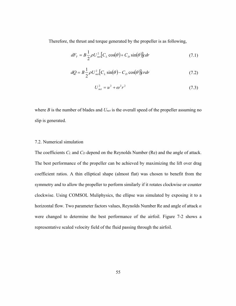
7.2. Numerical simulation ............................................................................................. 55

7.3. CAD model design ................................................................................................. 57

7.4. Experimental setup ................................................................................................. 57

7.5. Results and discussion ........................................................................................... 60

vi

CHAPTER Page

8. CONTROLLER DESIGN ............................................................................................ 65

8.1. Motor controller ..................................................................................................... 65

8.2. Vehicle controller stability ..................................................................................... 66

8.3. Electric circuit and communications ...................................................................... 67

9. CONCOLUSION AND FUTURE WORK .................................................................. 69

9.1. Conclusion ............................................................................................................. 69

9.2. Future work ............................................................................................................ 71

REFERNCES .................................................................................................................... 72

Appendix A 79

Appendix B 91

vii

LIST OF TABLES

Table Page

Table 2–1 .......................................................................................................................... 13

Table 3–1 .......................................................................................................................... 24

Table A–1.......................................................................................................................... 81

viii

LIST OF FIGURES

FIGURE Page

Figure 1-1 Flow diagram of the underwater vehicle design process. ................................. 2

Figure 2-1 Primary Node locations on the Juan de Fuca Ridge to provide power and data

communication. ................................................................................................................... 7

Figure 2-2 A network of underwater vehicles with sensors mapping the ocean floor to

enable physical, chemical and biological discovery. .......................................................... 8

Figure 2-3 Underwater vehicles to explore the deep ocean. (a) Alvin. (b) Sentry. (c)

Jason. ................................................................................................................................... 9

Figure 2-4 Basic componants of unmanned underwater vehicle. ..................................... 11

Figure 2-5 Current existing AUVs. (A) 690 AUV. (B) High Speed AUV. (C) Self-

Mooring AUV. (D) 475 AUV. .......................................................................................... 12

Figure 3-1 Energy density of several battrey technologies. .............................................. 16

Figure 3-2 Vehicle overall siz as the sum of propeller size and battery size. ................... 17

Figure 3-3 Miniaturized Underwater Vehicle divided into three independent major

sections. ............................................................................................................................. 18

Figure 3-4 Schematic figure of the deep-sea mUV, which shows the structure of the

vehicle with dimensions. ................................................................................................... 19

Figure 3-5 The relation between the propeller diameter and the mUV outer diameter.

Based on the chosen and calculated parameters, the smallest AUV outer diameter is about

15.3cm (6in) which corresponds to a propeller diameter of 4.0cm (1.575in). ................. 25

Figure 4-1 mUV and propulsion system schematics with forces acting on it. ................. 27

Figure 4-2 Free body diagram of the fin lift force acting on the mUV. ........................... 29

ix

FIGURE Page

Figure 4-3 The relation between the stationaty reference fram and the moving reference

frame of the mUV. ............................................................................................................ 30

Figure 5-1 Brushless DC motor exploded showing the electric steel stator core stack and

aluminum rotor with permanent magnets. ........................................................................ 33

Figure 5-2 A two dimentional drawing for the stator with nine slots using Solidworks. . 35

Figure 5-3 A two dimentional drawing for the rotor with 24 flat surfaces around the outer

diameter using Solidworks. ............................................................................................... 36

Figure 5-4 Schematics of the three-phase brushless DC motor with stator winding and

rotor magnets. ................................................................................................................... 37

Figure 5-5 A two dimentional drawing for the rotor-side-holders using Solidworks. ...... 38

Figure 5-6 The anatomy of the motor-thruster components exploded. ............................ 38

Figure 5-7 2D FEA model showing flux distribution and magnetic flux density in Tesla

with no-load at a spicific rotor position. ........................................................................... 39

Figure 5-8 Motor back EMF ploted as a function of the rotor position simulated by

COMSOL Multiphysics. ................................................................................................... 40

Figure 5-9 Schematic and experiment setup for the flywheel with bearing attached to the

sides and optical sensor to measure the speed of the wheel using LabVIEW. ................. 41

Figure 5-10 One of the experimental data of the flywheel rotational speed vs. time. ...... 42

Figure 5-11 Block diagram to show the process and the connection of the motor to

measure the motor torque constant. .................................................................................. 43

Figure 5-12 Schematic to show the experimental setup of the motor to measure the motor

toque constant (KT) through the input electric current (I) and the rotor speed (ω). ......... 43

x

FIGURE Page

Figure 5-13 One of the experimental data of the motor speed vs. electric current with a

linear regression fit. .......................................................................................................... 44

Figure 6-1 A schematic of the proposed method to insulate propulsion system. ............. 47

Figure 6-2 Oil-filled pressure housing unit to protect electronic components by

preventing corrosion and avoiding short circuits. (A) Housing design with shaft seal. (B)

Housing with a magnetic coupling drive. ......................................................................... 48

Figure 6-3 Propulsion system insice an oil filling pressure resistance housing prototyp. 49

Figure 6-4 Plastic housing 3-D printed to insulate the stator winding from getting wet. . 49

Figure 6-5 Pressure resistance housing CAD model. ....................................................... 51

Figure 6-6 FEA of the pressure resistance housing simulated with COMSOL

Multiphysics showing Von Mises. Stress in MPa ............................................................ 52

Figure 7-1 Free Body Diagram (FBD) of an airfoil (flat plate with a chord length c)

rotating about the axis of rotation with a speed ω. ........................................................... 54

Figure 7-2 A representative scaled velocity field results of COMSOL Muliphysics

simulation of the ellipse at Re = 100000 and α = 5o. ........................................................ 56

Figure 7-3 Lift over drag ratio of the airfoil for Re range of 5000 (lowest curve) to 50000

(heighest curve) at 5000 steps. .......................................................................................... 56

Figure 7-4 CAD drawing for (A) Ring-thruster with seven blades and 100o twist angle.

(B) Ring-thruster with three extended blads and 60o twist angle. .................................... 57

Figure 7-5 Schematics of the experimental setup to measure thrust and torque as function

of ring thruster speed. ....................................................................................................... 58

xi

FIGURE Page

Figure 7-6 Labview front panal to measure the motor speed, the motor current and the

force sensor. ...................................................................................................................... 59

Figure 7-7 Thrust experiemtnal resuts of a non-extended ring thruster with 5 blades and

120o twist angle. ................................................................................................................ 60

Figure 7-8 Therust experiemtnal resuts of an extended ring thruster with 4 blades and 60o

twist angle. ........................................................................................................................ 61

Figure 7-9 Torque experiemtnal resuts of an extended ring thruster with 4 blades and 60o

twist angle. ........................................................................................................................ 61

Figure 7-10 Experimental results of the thrust generated by the propeller plotted as a

function of the quantity 42d . ....................................................................................... 62

Figure 7-11 Experimental results of the propulsion system thrust as a function of the

input power. ...................................................................................................................... 63

Figure 7-12 Experimental results of the ring-propeller torque as a function of the quantity

52d ............................................................................................................................... 64

Figure 7-13 Experimental results of the propulsion system Torque as a function of the

input power. ...................................................................................................................... 64

Figure 8-1 Block diagram of the motor system showing a negative feedback control. .... 65

Figure 8-2 Anaheim Automation Brushless Speed Controller board mount with

connection diagram. .......................................................................................................... 66

Figure 8-3 Propulsion generator schematics. .................................................................... 67

Figure 8-4 Motherboard circuit design using Eagle CAD. ............................................... 68

Figure 8-5 Propulsion system electronic ciruit board. ...................................................... 68

xii

FIGURE Page

Figure A-1 MATLAB results of the optimal trajectory example of the mUV going from

initial position to the final position in 300 sec. ................................................................. 82

Figure B-2 Schematics of the experimental setup. ........................................................... 92

Figure B-3 Experimental Data of the AUV drag pressure vs. dynamic pressure. The

equation of the linear regression fit for this data is Pdrag = 3.75 Pdyn. The measured

frontal drag coefficient of the mUV is 0.267. ................................................................... 93

1

1. OBJECTIVE AND RESEARCH CONTRIBUTION

1.1. Objective

Earth is unique among the other planets due to the existence of water. The presence of the

three states of water offers a suitable environment for life to exist. The ocean environments

are inhabited by many microorganisms that fundamentally influence the ocean’s ability to

sustain life on Earth. In the past few decades, there has been an increasing effort to

understand the ocean and its existing life forms. However, the ocean remains a mystery

due to the lack of exploration technologies. Its harsh environment is complicated by the

absence of breathable oxygen, high pressure, low temperature and water salinity making it

challenging for human’s to study. The goal of this study is to develop a miniaturized

underwater vehicle for ocean exploration and to evaluate its feasibility and effectiveness

by optimizing a variety of parameters.

The objectives of the project include the following: i) Minimize (miniaturized) the

size of the underwater vehicle with propulsion while retaining its performance standards.

The size of underwater vehicles is related to many parameters such as propulsion

parameters, shape parameters, mission duration and onboard energy density. This objective

will address those parameters and use their relations to push the overall size of the

underwater vehicle to the minimum; ii) Design a propulsion system that can generate the

required thrust for the miniaturized underwater vehicle (mUV). The propulsion can be

integrated into the mUV without increasing its overall size. This objective will explain the

design process of fabricating a custom three-phase brushless DC motor with permanent

magnets rotor to generate the required rotor speed. iii) Insulate the vehicle and its

components to function in ocean environment. The issue of corrosion plays a major role in

2

underwater vehicle design due to the high water salinity. In addition, the deep ocean

environment introduces a high ambient pressure; hence, many underwater vehicles cannot

function properly. This objective will achieve an insulation method to protect the vehicle

from those issues; iv) Design a propeller to maximizer thrust and efficiency. In general,

underwater vehicle with propulsion requires a propeller to generate thrust. The

performance of the propeller plays a major role in the overall vehicle speed and power

efficiency. This objective will apply an improved method to design a propeller with high

efficiency to generate the maximum thrust.

The purpose of this project is to study the possibility of miniaturizing underwater

vehicles with some design constrains to function properly in an ocean environment.

Figure 1-1 shows the summary of this thesis by following the design steps for the major

components of the vehicle.

Figure 1-1 Flow diagram of the underwater vehicle design process.

3

1.2. Research Contributions

Underwater Vehicles is the key to exploring our ocean world in a much more efficient way.

However, the ocean remains immense and the task to explore every part of it remains

extremely difficult. This dissertation prospectus proposes the development of novel deep-

sea miniaturized underwater vehicle as a method to enable the ocean discovery. The value

of this proposal is emphasized by the innovative application of commonly available tools

that are immediately relevant to researchers interested in developing miniaturized deep-sea

compatible underwater vehicle.

Based on the projects results, all objectives have been successfully achieved. The

scientific contribution of this research include: firstly, underwater vehicle size

minimization with the constrain of traveling range. The task is to investigate the limit to

push the size of the vehicle to the minimum while allowing a minimum traveling range

performance. The result suggested that size of the vehicle depend mainly on the onboard

energy density. Secondly, underwater brushless three-phase DC motor with permanent

magnets was designed and fabricated to meet the demanded thrust generation of the

propulsion system. The brushless motor was structured to occupy the core of the

underwater vehicle. The significant of the brushless motor are: a) generating the required

forward or backward thrust to permit motion to the underwater vehicle; b) the brushless

motor has an inrunner rotor, which allow a new and easier method for stator electronic

insulation; c) the whole propulsion module is independent and it can be integrated into

other types of future underwater vehicles. Thirdly, the brushless motor was insulated using

a new method, which inspired from the existing underwater propulsion insulation methods.

This task suggests an insulation to the propulsion electronic parts such as the stator

4

winding, energy sources (battery pack), electronic circuits and wiring. The non-electronic

components were left outside the insulation such as the rotor, the permanent magnets and

the propeller. Finally, the propeller was designed to induce the performance and maximize

the overall vehicle efficiency. Blade element theory was applied to design several

underwater propellers. Each propeller was experimentally tested to investigate the

maximum thrust generated and its efficiency. The results suggested a maximum propeller

efficiency of 46%.

In my learning curve for the past five and half years, I have presented my work

progress, at least once a year, to the Biodesign Institute/Center for Biosignatures Discovery

Automation group. In November 2012, I was invited by The Motor and Motion Association

(SMMA) in St. Louis to attend a conference and present my designed underwater brushless

motor. In addition, a journal paper is in progress for submission with Ocean Engineering

Elsevier journal.

Merza, S. A., Thompson, A., Chao, J., & Meldrum, D. R. (2014). Brushless DC Motor with

a New Pressure Housing Design Approach for Underwater Propulsion System. Ocean

Engineering. In progress.

5

2. INTRODUCTION

The desire of understanding our ocean planet has increased drastically in the past two

decades due to global climate changes (Karl & Trenberth, 2003) and the improvements of

ocean technology systems (Kim, Choi, Lee, & jun Lee, 2014; Huang, Yang, Liu, &

Schindall, 2013; Ruiz et al., 2012; Gracias & Santos-Victor, 2000). Therefore, many

underwater vehicles were developed to perform certain tasks, which enable ocean

measurements and discovery (Eriksen et al., 2001;Yoerger, Jakuba, Bradley, & Bingham,

2007; von Alt, 2003). However, before describing the underwater vehicle technologies, a

step back must be taken to investigate the importance of the ocean and its influence on

our planet and lives.

2.1. Why the Ocean?

The Ocean is the "engine" that drives weather-climate systems from the ocean basins onto

the continents, directly affecting food production on land and the health of our planet. It

covers nearly 71% of the planet and it is considered the largest habitant for life. Our

understanding life’s existence was based on sunlight (photosynthesis). However, the deep-

sea has changed our prospective after the discovery of giant worms and clams near the

hydrothermal vents. This type of life has a chemosynthetic-base, which suggests the

possibility of life elsewhere in the cosmos (Maier-Reimer & Hasselmann, 1987;

Tunnicliffe, 1992)

According to National Oceanic and Atmospheric Administration (NOAA) the

biological productivity of the ocean plays a major role in global climate and carbon cycle

which is the source of nearly 50 percent of the Earth’s oxygen and 20 percent of the world

6

protein supply (Field, 1998). In addition, the ocean species are also a potential basis of

some medicines. (Tyson, Rice, & Dearry, 2004)

Life would not exist without our ocean. In fact, if planet Earth become without

ocean, it would look like planet Mars where there is no life exist in the form earth life.

Therefore, the ocean is vital to the health of our planet but remains virtually unexplored

due to the hostility environment to the human life. The lack of breathable oxygen, high

pressure encountered in the atmosphere, and unbearable low temperatures makes it

unsuitable for humans to be present at the deep-sea level. Therefore, many researchers seek

to understand a wide range of geological and biological phenomena by developing

technologies that enable deep-sea exploration. (Gage & Tyler, 1992)

2.2. Where in the Ocean?

The Ocean Observatories Initiative (OOI) aims to extend power and bandwidth into the

oceans. The OOI Regional Scale Nodes (RSN) has a Primary Infrastructure, which uses

cables to distribute power and support communication from land to the sea in and around

the Juan de Fuca Ridge. The cable is as 400km long and it provides a two-way

communications between the land and the sea (see Figure 2-1) (Isern & Clark, 2003). Axial

Seamount is the most robust volcanic system on the Juan de Fuca Ridge and it is

seismically, magmatically, and hydrothermally active.(Tivey & Johnson, 1990)

7

Figure 2-1 Primary Node locations on the Juan de Fuca Ridge to provide power and

data communication.

2.3. Ocean floor future research vision

Our ocean discovery aim is to have high quantity of sensors mapping different areas of the

ocean floor to preform simultaneous physical, chemical or biological measurements. The

next step is to develop miniaturized Underwater Vehicles (mUV)’s with a mission to swim

around the primary nodes or RSN and record measurements generated by the onboard

sensors. Those mUVs onboard small sensors modules and small devices are designed to

enable specific physical, chemical or biological measurements (such as temperature

sensors, PH level sensor, Oxygen sensor, single cell gene analyze, etc.), within the targeted

ocean floor. In addition, a network of mUVs can perform simultaneous physiological

measurements to cover areas in a form of grids and nodes (see Figure 2-2). However, each

individual mUV is limited with the amount of energy they require within one mission.

8

Figure 2-2 A network of underwater vehicles with sensors mapping the ocean floor

to enable physical, chemical and biological discovery.

2.4. Types of underwater vehicles

Many researchers seek to understand a wide range of geological and biological phenomena

by developing technologies, which enable deep-sea exploration. Of these technologies,

underwater vehicles were developed to study the deep ocean. Many deep-sea underwater

vehicles can be classified into two types.(Brown Jr & Hendrick, 1986; Yuh, 2000) The first

type is manned underwater vehicles such as Deep-Submergence Vehicle (DSV). For

example, Alvin (DSV) is a manned deep-sea research submersible. It dives 4.5 km below

the ocean surface and travel at a maximum speed of 2 knots. Its size is about 7.1 m x 2.6

m x 3.7 m and it weight about 17 tons. In addition, Alvin can have two scientists and one

9

pilot onboard.(Mavor, Froehlich, Marquet, & Rainnie, 1967) The second type is unmanned

underwater vehicles, which are known as Autonomous Underwater Vehicle (AUV), and

Remotely Operated Vehicle (ROV). AUVs are robots, which do not require input from an

operator. Sentry (AUV), for example, was designed to operate at depth of 5 km below the

ocean surface and travel at a maximum speed of 2.5 knots. Its specific task is to carry

devises for sampling and measuring purposes.(Martin, Whitcomb, Yoerger, & Singh,

2006; D. Yoerger, Bradley, Martin, & Whitcomb, 2006) Sentry’s dimension is 1.8 m x 2.2

m x 2.9 m. On the other hand, ROVs are tethered underwater robot vehicles. This type of

robot is usually operated by an operator on land or in the air. For example, Jason (ROV)

was design to access the deep ocean without leaving the deck of a ship. Its dimension is

1.8 m x 2.2 m x 2.9 m and its maximum traveling speed is 1.5 knot (see Figure 2-3).(D. R.

Yoerger & Newman, 1986; D. R. Yoerger, Newman, & Slotine, 1986; D. R. Yoerger, Von

Alt, Bowen, & Newman, 1986) Most of these types of deep-sea underwater vehicles were

developed to explore the ocean. However, most of them are limited in their exploration

capabilities, big, expensive and complicated to make and deploy.

Figure 2-3 Underwater vehicles to explore the deep ocean. (a) Alvin. (b) Sentry. (c)

Jason.

10

2.5. Unmanned underwater vehicle design philosophy

Most underwater vehicles were designed to fulfill a specific mission task. Unmanned

underwater vehicle should be capable of performing a task that human cannot do. However,

in most cases, cost becomes a factor where unmanned underwater vehicles overall cost is

cheaper or safer than human dive. In the case of deep-sea research, unmanned underwater

vehicles are the ideal technology selection. This is because of the high incompatible

pressure that human cannot stand within the deep-sea environment.

The unmanned underwater vehicle design structure must meet the criteria that the

missions demand. Most importantly, part of the vehicle space must be detected to hold a

payload. In addition, for some measurement devices requires a dry pressure housing space

to insure proper functionality. (T. Hyakudome, 2011)

The unmanned underwater vehicle should be made in the simplest form. The

vehicle should not require team of engineers and programmers to operate the vehicle. The

vehicle should have a simple interface where a technician with basic computer skills can

operate it.

2.6. Underwater vehicle system and components

The most basic underwater vehicle must have some kind of navigation system,

propulsion system and a dry, watertight environment to house onboard components.

(Poole & Clower, 1996)

11

Figure 2-4 Basic componants of unmanned underwater vehicle.

Underwater navigations can be classified into two classes. At the water surface,

GPS systems can be used to access highly accurate position data worldwide with up to

one-meter error. However, GPS radio frequency signal do not penetrate through water.

(Schelleng, Burrows, & Ferrell, 1933)Therefore, other positioning methods can be used

such as inertial motion unit (IMU) and Doppler velocity log (DVL). The IMU can

determine the vehicle orientation and the VDL can measure the vehicle speed relative to

the sea floor.(Rowe & Young, 1979) However, DVL systems are expensive and may not

be ideal for many applications. Other types of underwater navigation, while still

expensive, includes long baseline navigation (LBL). (Larsen, 2000) LBL is one of the

underwater acoustics positioning systems, which use a network of sea floor, mounted

baseline transponders as a reference points for navigation. Remotely operated vehicles

(ROV) can be navigated through visual landmarks or a compass. (Ramírez, Vásquez,

Gutiérrez, & Flórez, 2007)

Propulsion system is another important component of underwater vehicles. There

are different types of underwater propulsions that generate thrust to provide motion to the

12

vehicle. Propeller base propulsion is considered the most efficient method for underwater

long traveling range (Bellingham et al., 2010).

2.7. Current small underwater vehicles

The Autonomous Systems and Controls Laboratory (ASCL) at Virginia Tech focus on

novel research contribution toward autonomous systems control, estimation, decision

theory, the design of novel hardware, and the practical art of operating advance vehicles

in the field. ASCL designed four autonomous underwater vehicles with different

specifications. All four considered small and compact with a special specifications. The

four AUV’s principal characteristics are shown in Table 2–1. (Arafat, Stilwell, & Neu,

2006; Briggs, 2010; Petrich & Stilwell, 2011)

Figure 2-5 Current existing AUVs. (A) 690 AUV. (B) High Speed AUV. (C) Self-

Mooring AUV. (D) 475 AUV.

13

Table 2–1

Small Autonomous Underwater Vehicles desiged by Virginia Tech ASCL.

AUV Name Size (Length,

Diameter) in inches

Max Depth

in meter

Speed in

knots

Endurance

in hours Description

690 AUV (81,6.9) 500 4 24 Bathymetric surveys

High Speed AUV (36,3) N/A >15 N/A Small and fast

Self-Mooring AUV (89,6.9) 500 4 N/A Mooring itself on the seafloor

475 AUV (34,4.75) N/A 3 8 Enable research and development

objectives

13

14

3. MINIATURIZED UNDERWATER VEHICLE DESIGN

Small ocean instrument platforms offer a much higher measurement resolution in space

and time. (Dickey, 1991; Eriksen et al., 2001) In many cases, ocean research is not

constrained by the overall underwater vehicle size. However, for some specific research

purpose, the overall size of the underwater vehicle plays a major role in the discovery

mission. (Behar, Bruhn, & Carsey, 2003) For example, astrobiology researchers seek to

study the microbial ecosystems under the ice in Earth’s Polar Regions. In many cases,

creating large opening is required to allow access to the water to enable benthic studies.

Smaller size underwater vehicles can enable discovery in tiny places were large vehicle

cannot. In some underwater research cases, multiple vehicles are necessary to perform

simultaneous sensor measurements within different nearby areas. The cost of designing,

fabricating and deploying underwater vehicles could play a major factor. Therefore, the

size of each robot vehicle will be optimized to reduce ocean specific material costs.

However, each robot must have the capability of carrying sensor devices (payloads),

travel long ranges, be energy efficient and rechargeable, controllable, stable and easy to

develop.

Several small underwater deep-sea sensors devices were available to measure

physical and chemical parameters such as temperature, pH level and oxygen concentration.

Miniaturized underwater vehicles were needed to carry the sensors around the ocean and

record data to enable ocean discovery.

15

3.1. Energy sources and limitations

In many cases, energy source is the fundamental factor for deep-sea underwater devices.

For most devices, the lifetime of operation is limited by the energy storage. There are

three main energy types such as nuclear fusion, chemical and electrochemical.

(Bradshaw, Hamacher, & Fischer, 2011; Winter & Brodd, 2004; Yang et al., 2011)

Fusion batteries have the highest energy density. However, they are not compact and

dangerous due to spew radioactive materials. The second highest energy density is the

chemical energy type. However, the chemical energy type requires oxygen for

combustions and is not suitable for ocean environment. Electrochemical energy type is

the lowest energy among these sources. However, there are several advantages of this

type of energy storage. First, they are clean and green energy. Second, it can be easily

converted to other forms of energy. Third, they are inexpensive. Fourth, they can be

rechargeable for several usage cycles. Most importantly, they can be easily transmitted to

various location conveniently and efficiently. (Chalk & Miller, 2006) Based on these

factors, the electrochemical energy is the best choice for underwater application. In

addition, Li-ion batteries are the most common method of energy source for long

traveling underwater vehicles, (see Figure 3-1). (Bradley, Duester, Liberatore, &

Yoerger, 2000) In addition to the recharging ability, they can be enclosed with oil to

protect it from the high pressure and the saltwater. (T. Hyakudome, Yoshida, Ishibashi,

Sawa, & Nakamura, 2011)

16

Figure 3-1 Energy density of several battrey technologies.

3.2. Underwater vehicle size optimization

The mean ocean current speed near the sea floor and west of Oregon (depth between

2700 m to 2900 m) is about 2 cm/s with a maximum speed of 6 cm/sec. The mean current

speed from depth 725 m to 1700 m, range from 5 to 20 cm/s with a maximum of 20-40

cm/s depend on the water depth. (Korgen, Bodvarsson, & Kulm, 1970)

There are limitations associated with the size of the mUV which can lead to

certain challenges. Beside the salinity of the ocean water, the pressure at the seafloor is

usually high. For example, 2000m below the sea level, the pressure is as high as 3000psi.

Therefore, certain mUV component modules, such as the propulsion system, will

require pressure-proof housing and corrosion resistance materials to ensure the

17

functionality of the mUV. The most critical and challenging step of developing a mUV is

to overcome the ocean current against which the mUV swims against.

Therefore, the size of the mUV is limited by the energy density. For example, the

smaller the propeller, the more power (i.e. larger battery) is required to overcome the

ocean current. However, minimizing the battery size also requires a larger propeller.

Therefore, the mUVs propellers and the batteries must be developed at optimum sizes

(see Figure 3-2).

Figure 3-2 Vehicle overall siz as the sum of propeller size and battery size.

In order to complete this optimization, specific underwater vehicle design

principles and structure must be applied. For a long-range traveling underwater vehicle, a

torpedo shaped vehicle is the most common choice to improve the aerodynamic stability

of the vehicle and to minimize drag. Furthermore, the propulsion system of the vehicle

can be designed such that the driving motor is imbedded to the vehicle core. This allows

18

easier process to insulate the motor stator and its electronic circuits to prevent from direct

contact to the highly pressurized ocean water.

The miniaturized underwater vehicle is composed of three independent sections.

First, the front section is dedicated to carrying ocean measurement devices such as a

camera, temperature measurement device, biological cell/bacteria analyzers (PCR), etc.

Second, the propulsion system occupies the middle section of the vehicle. Finally, the

rear section of the vehicle is reserved for the maneuvering system. Figure 3-3

demonstrates the schematics of the vehicle.

Figure 3-3 Miniaturized Underwater Vehicle divided into three independent major

sections.

19

3.2.1. Continuous optimization problem

There are three major components such as the motor-thruster, battery and hotel load

which adopt the overall underwater vehicle size. The frontal diameter of the vehicle (D)

and the propeller diameter (d) are the two factors that determinate the traveling range and

performance of the underwater vehicle. In addition, the length of the vehicle can be

represented as direct proportional function of the mUV frontal diameter (for example,

2D). Therefore, the size of the vehicle can be represented with the two parameters D and

d (see Figure 3-4).

2322

3dDVmUV

. (3.1)

Figure 3-4 Schematic figure of the deep-sea mUV, which shows the structure of the

vehicle with dimensions.

20

The hollow cylindrical motor size is part of the mUV overall size. I can assume a

motor with a length L that has an outer diameter of the average length of the propeller

diameter d and the mUV outer diameter D. This assumption is appropriate to insure the

ability of the motor to fit inside mUV.

. (3.2)

The size of the battery can be represented as the ratio of the watt-hour (Power P

and time t) to the energy density VBE .

VBB E

PtV . (3.3)

The extra space known as Hotel Load or Payload volume VH such as flotation

materials, housing materials and dead volumes can be represented as a fraction of the

overall volume of the vehicle VmUV.

. (3.4)

Therefore, the overall volume of the mUV can be expressed as the sum of all

three volumes VM, VB and VH,

HBMmUV VVVV . (3.5)

By substituting the equations (3.1), (3.2), (3.3), and (3.4) into equation (3.5) I get,

2322

22

31

44dD

E

Ptd

dDL

VB

. (3.6)

2

2

44d

dDLVM

10, mUVH VV

21

The power of the mUV can be represented as the output power of the motor times the

efficiency η.

IkP T , (3.7)

where Tk is the motor torque constant, I is the motor rated electric current and ω is the

rotation speed of the rotor.

I can use the propeller thrust force TF equation and the drag force DF equation to relate

the propeller speed to the vehicle speed.

ACUF DD2

2

1 , (3.8)

42dCF TT , (3.9)

where ρ is the fluid density, DC is the drag coefficient, A is the frontal surface area and

TC is the thrust coefficient.

In steady state motions, assuming no external hydrodynamics effects and laminar

flow, the two forces are equal. Therefore, the relation between the mUV velocity U and

the propeller speed ω is,

T

D

C

C

d

UD

22 2

. (3.10)

Substituting equations (3.10) into (3.7) lead to,

T

DT

C

C

d

IUDkP

22 2

. (3.11)

22

The frontal area A of the mUV can be expressed as πD2/4. I combine equations

(3.6) and (3.11) to get the relations between the mUV propulsion and battery parameters

and its shapes parameters.

2322

22

2

31

2244dD

C

C

Ed

IUDtkd

dDL

T

D

VB

T

. (3.12)

Equation (3.12) represents the equality constraint subject to the domain,

22min dD , (3.13)

with the inequality constraint,

0 dD . (3.14)

The constant α can be approximated by using the following buoyancy balance

equation.

gVgmmmF mUVHBMnet , (3.15)

where netF is the buoyancy force pointing up or down, Mm is the mass of the motor, Bm is

the mass of the batteries, Hm is the mass of the hotel load and g is the gravitational

acceleration.

The mass of the battery can be calculated from its specific energy ( mBB EPtm / ).

The mass of each other sections can be computed using the product of its equivalent

density and the volume (m = ρV). To make the mUV neutrally buoyant, the net force

must equal to zero. Therefore, after using equations (3.1), (3.2), (3.3), (3.4), and (3.11)

equation (3.15) becomes,

23

23222

22

32244dD

C

C

dE

IUDtkd

dDLH

T

D

mB

TM

, (3.16)

3.3. Results

Before minimizing the continuous optimization problem equations (3.12), (3.13), (4.2),

and (3.16) require certain parameters, which were determined by assumptions, lookup

tables and preliminary experiments. Table 3–1 represents the value of each parameter

needed for equation (3.12) and (3.16).

24

Table 3–1

Miniaturized Underwater Vehicle parameters.

Parameter Notation Value Unit

Battery Volumetric Energy Density VBE 1 MJ/L

Battery Gravimetric Energy Density mBE 0.37 MJ/kg

Vehicle Speed U 1 m/s

Swimming Time t 24 hour

Electric Current I 2 A

Motor Length L 2.625 inch

Motor constant Tk 0.015 N.m/A

Motor Equivalent Density M 2700 Kg/m3

Efficiency η 0.30 unitless

Drag Coefficient DC 0.267 unitless

Thrust Coefficient TC 0.10 unitless

After plugging the parameter from Table 3–1, equations (3.12), (3.13), (3.14), and

(3.16) were solved using online Wolfram Alpha computational knowledge engine. The

result suggested a vehicle diameter of 0.154 m and propeller diameter of 0.041 m.

Using the parameter from Table 3–1, the relation between D and d were plotted as

shown in Error! Reference source not found.. In this case, the outer diameter of the

25

mUV cannot be smaller than about 6 inch (0.153 m). Therefore, the appropriate propeller

size is 1.575 inch (0.04 m).

Figure 3-5 The relation between the propeller diameter and the mUV outer

diameter. Based on the chosen and calculated parameters, the smallest AUV outer

diameter is about 15.3cm (6in) which corresponds to a propeller diameter of 4.0cm

(1.575in).

26

3.4. Discussion and conclusion

The size of the mUV was determined to have a diameter of six inches and twelve inches

in length. The ring-propeller diameter cannot be smaller than 1.6 inches otherwise the

vehicle will not meet the required performance. These results were determined through

the analysis, which consider a linear motion with the assumption of continuous maximum

vehicle speed with no additional disturbance to the system. In addition, the energy source

of the mUV is fully dedicated to the motor system only. Heat and power losses were not

taking into the account in order to simplify the miniaturization process.

It is important to realize that the mUV outer diameter must be greater than the ring-

propeller diameter. This will lead the increase in the vehicle rooming size, which leads to

an easier way to include extra components or extra energy sources such as batteries.

However, the ratio of the mUV outer diameter to the ring-propeller squared diameter

influence the relation between the ring propeller speed and the vehicle forward speed.

This leads to a chance in the vehicle performance and range shortage.

The future of this type of miniaturized underwater vehicle can occupy not only our ocean

but it might be a method to discover outer space planets, which contains liquid water such

as Europa. The mUV can also be a module to integrate into a larger underwater vehicle

system to act as the propulsion system source.

27

4. VEHICLE EQUATION OF MOTIONS

The model base of the vehicle can be described using the equation of motion. Assuming

naturally buoyant and a linear motion for the mUV with fins, using a propeller on a

torpedo shaped vehicle and no external flow disturbances. The force and moment acting

on the mUV are shown in Figure 4-1.

Figure 4-1 mUV and propulsion system schematics with forces acting on it.

Therefore, the equation of the propeller speed ω driven by the motor with a motor

constant TK is,

netT IKQbdt

dJ

(4.1)

where J is the moment of inertia along the x-axis, b is the bearing damping coefficient, Q

is the propeller torque and Inet is the net electric rated current applied to the motor.

28

Due to the thrust FT generated by the propulsion system, the mUV with a mass m will

travel at a speed u.

TD FFdt

dum (4.2)

where FD is the drag coefficient of the vehicle.

Assuming no cavitation, neglect frictional losses, incompressible fluid, no gravity

effects, and perfect propeller symmetry the parameter Q, FT and FD can be expressed as,

52dCQ Q , (4.3)

42dCF TT , (4.4)

AuCF DD2

2

1 , (4.5)

where CQ, CT and CD are the propeller torque constant, propeller thrust constant and

mUV drag constant, respectively.

The equations (4.3), (4.4) and (4.5) will give positive values since they represent the

magnitude of the torque and forces. However, in order to incorporate the direction of the

torque and the forces, the signs of the propeller rotation speed and the mUV velocity

must be carried along the Ordinary Differential Equations (ODE) shown in equation (4.1)

and (4.2). Therefore, the square terms of u and ω can be broken down as the product of

itself and its absolute value (i.e. uuu 2 and 2 ).

The yaw of the mUV can be controlled by the fins. This will enable the mUV to move

within x-axis and y-axis. Figure 4-2 shows the lift force generated by the fin and acting

on the mUV. According to (Prestero, 2001), the lift force can be calculated using blade

element theory.

29

2

2

1uHCF LL , (4.6)

where LC is the lift coefficient of the fin, H is the surface area of the fin, and δ is the

angle between the fin and forward axis of the mUV.

Figure 4-2 Free body diagram of the fin lift force acting on the mUV.

The moments generated by both fins (above and below the mUV) are l distance

away form center of mass. The two fins will allow the mUV to yaw and introduces a

rotational speed Ω along the z-axis. However, this rotation is not generated unless the

vehicle is moving. Therefore, the yaw of the mUV equation can be represented as,

uupfdt

dI z

(4.7)

where zI is the moment of inertia of the mUV along the z-axis, f is the damping

coefficient, and p is the constant HlCL .

30

Figure 4-3 The relation between the stationaty reference fram and the moving

reference frame of the mUV.

For a vehicle with a local coordinates (r,φ), moving forward at a velocity u and

rotating at an angular velocity ω generated by fins at a distance l form the center of mass

of the vehicle.

rl

uu

ˆ,

. (4.8)

Assuming an initial velocity Vo and defined as,

jioy

oxo V

VV

ˆ,ˆ

. (4.9)

The transformation from the local frame to the global frame is,

cossin

sincosR . (4.10)

31

Therefore, the transformation of the mUV velocity 'rV from the local coordinates

to the global coordinates is,

uVVr R 0' . (4.11)

The vehicle yaw angle can be expressed as,

dt

d. (4.12)

Assuming,

ji

r

dt

dydt

dx

V

ˆ,ˆ

'

. (4.13)

the x and y position of the mUV are,

sincos luVdt

dxox , (4.14)

and cossin luVdt

dyoy . (4.15)

Choosing u, ω, , , x and y to be state variables ( 1x , 2x , 3x , 4x , 5x and 6x )

respectively. In addition, Inet and S to be the inputs 1u and 2u . Hence, the state space

representation can be rewritten as,

32

4351416

4351415

34

211313313

12122222212

111222111

cossin

sincos

xxaxxVx

xxaxxVx

xx

uxxbxax

ubxxaxax

xxaxxax

oy

ox

, (4.16)

M

pb

J

Kb

laM

fa

J

dCa

J

ba

m

ACa

m

dCa

T

Q

D

T

31

21

51

31

5

22

21

12

4

11

2

, (4.17)

33

5. BRUSHLESS THREE-PHASE DC MOTOR DESIGN

5.1. Introduction

The motor is the most important component of the mUV. It plays a major role in the

propulsion system. However, the size of the motor and its performance must meet the

criteria of the mUV. An inrunner three-phase brushless permanent magnets DC motor

with Hall Effect sensors was designed to fit inside the mUV’s core. The desired

dimensions of the motor involve a 3 inch outer diameter and 1.25 inch length. The rotor

is designed to fit a long ring propeller 1.625 inches in diameter and 2.625 inches in

length. The motor is composed of a stator with nine slots and three pull pair magnets with

an air gap thickness of 1.15mm. Two thin-section bearings were used to hold the rotor

and allow it to rotate freely (see Figure 5-1).

Figure 5-1 Brushless DC motor exploded showing the electric steel stator core stack

and aluminum rotor with permanent magnets.

34

5.2. Stator development

Nine slots brushless DC motor was designed using Solidworks (V.2011, Dassault

Systems). A section of the stator with dimensions is shown in Figure 5-2 . A 1.25 inch

high stator core was assembled from stacks of electrical steel laminations that have a high

relative magnetic permeability (about 4000). The purpose of the lamination stack is to

reduce the eddy-current and improve overall motor efficiency (Atallah, 1992; Greig &

Sathirakul, 1961). The assembly of the stator core was formed from those electric steel

laminations with a skew angle of 20o to reduce torque cogging and enable smooth motor

rotation startup (Islam, 2009; Yeadon, 2001). Skewing complicates numerical

electromagnetic analysis. The simulation is usually time consuming since it requires 3-D

finite elements analysis (FEA) or 2-D models with many slices (Holik, Dorrell, Lombard,

Thougaard, & Jensen, 2006). The stator core was insulated using a specific epoxy stator-

insulation material. The custom cuts of the stator laminations were fabricated by Proto

Lamination Inc. and assembled by Winding Inc.

Each tooth was winded by hand with 25 clockwise turns in the form of

(ABCABCABC) using 22 gauge copper wire to form three-phase stator windings. During

the winding, each phase was tested for short circuit using a multimeter. Wye

configuration was formed out of the three-phases. In addition, three Hall Effect sensors

were placed (with 40o a part from each other) on to the stator to control the rotation speed

of the rotor. The brushless motor speed was controlled using a brushless speed controller

(MDC010-050101, Anaheim Automation).

35

Figure 5-2 A two dimentional drawing for the stator with nine slots using

Solidworks.

5.3. Rotor development

The rotor is in the shape of hollow cylinder and is made of aluminum with 24 magnet

blocks assembled around it. The aluminum hollow cylinder is 2 inches long with a 1.90-

inch outer diameter and a 1.625-inch inner diameter. The outer diameter of the rotor was

shaved in the longitude direction evenly and at a width of 1/4 inches. Each magnetic

block is 2 inches long, 1/4 inches wide and 1/16 inches thick, which is magnetized

through thickness. Each four magnets were put together in the same polarity to form one

36

magnetic pulling force. All magnets were mechanically fixed to the aluminum cylindrical

rotor using two aluminum rotor-side-holders on each side.

Figure 5-3 A two dimentional drawing for the rotor with 24 flat surfaces around the

outer diameter using Solidworks.

37

Figure 5-4 Schematics of the three-phase brushless DC motor with stator winding

and rotor magnets.

5.4. Rotor side-holders design

The magnets were put together around the aluminum rotor and mechanically fixed using

two rotor-side-holders. Figure 5-5 shows the two dimensional drawing for the rotor-side

holder-part using Solidworks. The two side-holders are assembled with the rotor and the

magnets using 2-56 size screws to form the rotor magnets of the motor. The rotor is held

by two commercially available thing-section-bearing through each rotor-side-holder.

Figure 5-6 shows the anatomy of the brushless motor. It also shows the actual

brushless motor after the assembly. Side-motor-housings were machined to hold the

stator and the thin-section-bearing together for motor testing purposes.

38

Figure 5-5 A two dimentional drawing for the rotor-side-holders using Solidworks.

Figure 5-6 The anatomy of the motor-thruster components exploded.

39

5.5. Motor numerical simulation

The motor cross-section was simulated in two-dimensional COMSOL Multiphysics

simulation package. The assumption of skewing was neglected and the stator core and

rotor core without losses. The model was simulated with the Rotating Machinery and

Magnetic (rmm). A constant rotor speed (1000 RPM) was applied to the rotor to study the

corresponding generated back EMF. The simulation computed the flux distribution and

the magnetic flux density are shown in Figure 5-7. In addition, the back EMF as a

function of rotor position is plotted in Figure 5-8. The motor voltage constant was

calculated to be 0.015 V.s/rad.

Figure 5-7 2D FEA model showing flux distribution and magnetic flux density in

Tesla with no-load at a spicific rotor position.

40

Figure 5-8 Motor back EMF ploted as a function of the rotor position simulated by

COMSOL Multiphysics.

5.6. Damping coefficient of the thin-section-bearings

The damping coefficient can be estimated using the equation of motion equation (4.1) for

the brushless DC motor. Since there is no propeller or actual load, the torque resistance is

zero. In addition, without the brushless DC motor, the input electric current variable is zero

as well. The ODE becomes J

b and it can be solved which represent an exponential

decay equation.

tJ

b

et

0 (5.1)

The rotational speed can be described as a function of time curve as a line such that

the slope m is the derivative of ω(t) at time zero and the y-intercept as the initial rotational

41

speed ω(0). However, in order to get good linear regression fit to the curve, a high value

for the moment of inertia (i.e. high time constant) must be chosen.

0mJ

b (5.2)

The experiment was performed using a flywheel held by the bearings on both sides.

The rotational speed was measured using a Photodiode which measure the frequency of

light intensity passing through the checkerboard aligned at the boundary of the wheel (see

Figure 5-9).

Figure 5-9 Schematic and experiment setup for the flywheel with bearing attached

to the sides and optical sensor to measure the speed of the wheel using LabVIEW.

A LabVIEW user interface was developed to generate the data. This data was

analyzed which shows a damping coefficient of 1.42 × 10-4 ± 0.0965 × 10-4 with 95.4%

certainty (see Figure 5-10).

42

Figure 5-10 One of the experimental data of the flywheel rotational speed vs. time.

5.7. Motor torque constant experiment

The brushless motor with Hall-Effect sensors and a speed controller were assembled and

put through testing to measure its torque constant KT. A 0.05 ohms shunt resistor

(MP930-0.050-1%, CADDOCK) was added in series between the power supply (30 V)

and the motor controller in order to measure the input DC current flowing through by

measuring the potential voltage drop around it using a National Instrument Data

Acquisition (DAQ) card (6035E, National Instruments) . In parallel, the rotor position θ

as a function of time was measured by recording the potential drop across one of the

Hall-Effect sensors using the same DAQ card. A schematic of the experiment setup is

shown in Figure 5-11. Using LabVIEW (Version 8.6, National Instruments), the signals

were recorded for different reference speed inputs (Speed Knob). The measured DC

current, Inet, was plotted as a function of the rotor rotational speed ω.

43

Figure 5-11 Block diagram to show the process and the connection of the motor to

measure the motor torque constant.

The current was measured using an ammeter and the rotational speed was

measured using Hall Effect sensors (see Figure 5-12).

In a steady state with no torque load, equation (4.1) can be simplified as,

netT I

b

K (5.3)

Figure 5-12 Schematic to show the experimental setup of the motor to measure the

motor toque constant (KT) through the input electric current (I) and the rotor speed

(ω).

44

The experiment was performed and the rotor rotational speed ω was measured

against the input electrical rated current Inet. The motor torque constant was calculated

from the slope to be 0.014 N.m/A (see Figure 5-13). This value was obtained after

performing a small experiment to determine the damping coefficient of the thin-section

bearings b.

Figure 5-13 One of the experimental data of the motor speed vs. electric current

with a linear regression fit.

45


The three-phase brushless DC motor with permanent magnets was designed and

fabricated to become part of the propulsion system of the miniaturized underwater

vehicle. The most critical part of this design was the stator and the stator winding. The

winding process was not only time consuming but also critical. The copper wire required

to be winded without necking or bleeding the wire insulation. After each tooth winding,

the wire were inspected to short circuit. After each phase winding, the resistance and the

inductance were measured and confirmed to match the other phases.

The motor torque constant was determined numerically and experimentally to be

about 0.014. The measured data suggested a linear relationship between the rotor speed

and the input electric current. The torque constant can be improved by modifying the

stator structure. It can also be improved by increasing the number of wire turns through

each stator tooth. However, the winding was done by hand which permit room for error

and uneven distributions throughout the stator. Plan is to use machines to wind the stator,

which not only give a homogenous distribution, but also allows increasing the number or

turns.

46

6. VEHICLE INSULATION PRESSURE HOUSING DESIGN

6.1. Introduction

Many long traveling range underwater vehicles have a torpedo shaped vessel. This shape

improves the aerodynamics and motion energy required for the underwater vehicle (Davis,

Eriksen, & Jones, 2002). Our proposed torpedo shaped can be described as three assembly

segments. The first segment is the frontal area. This segment is considered the hotel load

segment where all the underwater sensors and measurement devices can be carried by the

underwater vehicle. The second segment is the middle part with a hollow cylinder shape.

This segment is the most critical part since it has the propulsion system and all electronics

components stored inside the cylinder. The third segment is dedicated for the navigation

system. It also includes the fins and necessary modules to enable the mUV with the

capability of turning.

6.2. New pressure housing design technique

A method is proposed to design an underwater thruster with a pressure-housing insulator

specifically applied to an inrunner three-phase brushless DC motor stator winding. The

pressure-housing wall is situated through the air gap between the stator and the rotor

magnets (see Figure 6-1). The wall thickness of the pressure housing must be thinner than

the air gap between the rotor and stator. In addition, a ring thruster is attached directly to

the hollow, cylindrically shaped rotor magnets.

47

Figure 6-1 A schematic of the proposed method to insulate propulsion system.

This new configuration was inspired by the current methods of deep-sea underwater

housing designs. Figure 6-2 shows the most common types of oil-filled pressure housing.

A motor can be encapsulated inside an oil-filled pressure-housing unit with a rotor shaft

sticking out through a radial shaft seal (Figure 6-2A). A shaft seal usually is composed of

an auxiliary lip that protects the primary sealing lip from leaking oil out or leaking seawater

in (Sasdelli, 1971). This type of seal may not be practical in high-pressure environments

such as the deep-sea (Tonder, 1992). However, it can work with the existence of pressure

balancing modules (Allen, 1997). In addition, this type of pressure housing and sealing

become more challenging and expensive as the water depth increases (Jahnke, 1989).

Figure 6-2B is another type of pressure housing design; however, it does not require a shaft

seal. The rotor shaft remains inside the pressure housing. The motion is transmitted through

the pressure-housing wall by a magnetic coupling drive. This concept works by aligning

opposite magnetic poles to generate attraction and repulsion forces between two hubs,

causing several magnetic poles to transmit torque from one magnet hub to the other. The

48

disadvantage of this type of coupling is that without careful alignment, vibrations will be

present which cause power transmission reductions and poor efficiency (Post, 1999).

Figure 6-2 Oil-filled pressure housing unit to protect electronic components by

preventing corrosion and avoiding short circuits. (A) Housing design with shaft seal.

(B) Housing with a magnetic coupling drive.

The propulsion system must be insulated and filled with syntactic foam and oil to prevent

the system electronics from the ocean water as it can short out the circuit due to the high

conductivity in the salty water. In addition, the housing material of this segment must be

compatible with the deep-sea environment to prevent material failure such as cracking and

corrosion. Syntactic foam is a composite material of epoxy and ceramics. It is known for

its strength and low density, which ideal for deep-sea application. This material often used

to balance the overall vehicle specific density and drive it to naturally buoyant.

49

Figure 6-3 Propulsion system insice an oil filling pressure resistance housing prototyp.

For underwater motor testing, a plastic (Vero white) housing was three-dimensional

printed (see Figure 6-4). This housing can insulate the entire stator winding and prevent

the electronics from getting wet.

Figure 6-4 Plastic housing 3-D printed to insulate the stator winding from getting

wet.

50

6.3. Deep-sea propulsion system pressure housing

In order to have a compatible deep-sea vehicle, certain criteria must be met. The most

important factor is pressure resistance. The deep ocean environment has high pressures,

which vary and depend on the depth from sea levels. For example at 3000 m depth, the

pressure can get as high as 6000 psi. The middle section, (i.e. the propulsion system) is

considered one of the critical sections due to sensitivity of its contents to high pressures

and water salinity. The propulsion system is composed of a brushless DC motor,

bearings, a propeller, batteries, electronic circuit boards and connecting wires. All of the

propulsion systems except the propeller, bearings, and rotor magnets must be protected

from high pressure and ocean water. Therefore, a pressure resistance oil filled housing is

necessary to prevent the propulsion system components from malfunctioning.

To design such housing, certain steps are necessary to be followed.

Design the CAD model of the deep-sea housing (Pressure vessel). Figure 6-5

proposes the pressure resistance housing structure.

Select a deep-sea compatible material to fabricate the housing with, such as an

aluminum alloy 5086.

Perform a FEA simulation to determine the failure points. See Figure 6-6.

Iterate the design and re-simulate the FEA model with the new geometry to

ensure no failure mode acquire.

Enable traditional deep-sea surface treatment of the aluminum alloy by anodizing,

TUFRAMR, electrolysis nickel plating, electroless nickel-plating, and painting.

51

TUFRAMR is a technique to make a surface enhancing coating of General

Magnaplate.

Assemble the propulsion system and integrate into the housing.

Fill with oil and syntactic foam to balance buoyancy in the water.

Seal the housing.

Test propulsion system inside a deep ocean simulator. Pressure testing facility in

San Diego (www.deepsea.com) is the ideal place for this test.

Iterate the design and repeat the process again until satisfactory results are

achieved.

Figure 6-5 Pressure resistance housing CAD model.

52

Figure 6-6 FEA of the pressure resistance housing simulated with COMSOL

Multiphysics showing Von Mises. Stress in MPa


Ideally, a propulsion system must be insulated and filled with non-conductive fluid

composing of a specific density lower than one, in order to achieve natural buoyancy. In

addition, the pressure housing material must be compatible with the sea environment in

order to prevent corrosion. However, in shallow water the environmental pressure is

insignificant, leaving the purpose of the housing to ensuring circuit functionality. In

contrast, the ambient pressure in the deep-sea environment is usually high. Therefore, the

pressure housing must be made of a strong, non-corrosive material such as aluminum

alloy 5086 with a minimum required wall thickness. The proposed pressure housing

method is simple. The housing wall thickness can be modified to prevent failure.

However, with this method, the wall thickness through the air gap is limited. The

53

cylindrically shaped stator can become a support for the thin housing wall, which

prevents it from deflection. The deep-sea pressure housing using this method will be

designed and analyzed in future work and it will not be discussed in this paper.

For underwater motor testing, the pressure housing was three-dimensionally printed using

a plastic material (VeroWhite). The housing is composed of the main body as well as a

cover; the cover seals the housing using a silicon glue and an O-ring. This specific

housing was tested and is capable of insulating the entire stator winding in order to

prevent water interference with the electronics.

54

7. PROPELLER OPTIMIZATION

7.1. Introduction

Underwater vehicle thrusters have a major impact on the vehicle system dynamic. The size,

shape, and speed of any propeller dominate the overall performance in terms of trust and

torque generated. (Manwel, McGowan, & Rogers, 2002) The shape of the blade cross-

section and its orientation dictate the efficiency of the propeller. For a traditional propeller

with an almost flat plate shaped blade cross-section, the lift and drag forces can be shown

in the free body diagram (FBD) in Figure 7-1. The airfoil rotating about the axis of rotation

at an angle θ – α generates a lift and drag forces (dFL and dFD). The vertical velocity of the

airfoil can be described as the product of the propeller rotational speed ω and the radial

distance r between the airfoil section and the center of the propeller. The horizontal velocity

of the propeller is denoted as u.

Figure 7-1 Free Body Diagram (FBD) of an airfoil (flat plate with a chord length c)

rotating about the axis of rotation with a speed ω.

55

Therefore, the thrust and torque generated by the propeller is as following,

cdrCCUBdF DLnetT sincos2

1 2 (7.1)

crdrCCUBdQ DLnet cossin2

1 2 (7.2)

2222 ruU net (7.3)

where B is the number of blades and Unet is the overall speed of the propeller assuming no

slip is generated.

7.2. Numerical simulation

The coefficients CL and CD depend on the Reynolds Number (Re) and the angle of attack.

The best performance of the propeller can be achieved by maximizing the lift over drag

coefficient ratios. A thin elliptical shape (almost flat) was chosen to benefit from the

symmetry and to allow the propeller to perform similarly if it rotates clockwise or counter

clockwise. Using COMSOL Muliphysics, the ellipse was simulated by exposing it to a

horizontal flow. Two parameter factors values, Reynolds Number Re and angle of attack α

were changed to determine the best performance of the airfoil. Figure 7-2 shows a

representative scaled velocity field of the fluid passing through the airfoil.

56

Figure 7-2 A representative scaled velocity field results of COMSOL Muliphysics

simulation of the ellipse at Re = 100000 and α = 5o.

Figure 7-3 Lift over drag ratio of the airfoil for Re range of 5000 (lowest curve) to

50000 (heighest curve) at 5000 steps.

57

7.3. CAD model design

Several CAD model propellers were created with different twist angles and blades number

then three dimensionally printed using 3D printer (see Figure 7-4). Sixteen propellers with

combinations of (4, 5, 6, and 7) blades and (60, 80, 100, and 120) degrees were made.

Another set of four propellers were made with extended three and four blades with 40o and

60o twist angles (see Figure 7-4) which should perform better aerodynamically. Each

propeller was tested underwater with different speeds. The results are going to be shown

in the Experiments and Results, Thrust and Torque coefficient section.

Figure 7-4 CAD drawing for (A) Ring-thruster with seven blades and 100o twist

angle. (B) Ring-thruster with three extended blads and 60o twist angle.

7.4. Experimental setup

Figure 7-5 shows the schematics of the experimental setup for both cases of thrust and

torque measurements. The structure stand was constructed from T-Slots beams

58

(47065T101, McMaster-Carr) to hold the motor in both configurations (thrust and

torque). This method was adopted from (Healey et al, 1995).

Figure 7-5 Schematics of the experimental setup to measure thrust and torque as

function of ring thruster speed.

Using structural mechanics, I can determine the relationship between the thrust

(or torque ) and the compression or the tension force in the sensor.

ST F

ba

aF

sin (7.4)

SFaQ sin (7.5)

where SF is the force measured by the load cell.

The trust and torque constants (CT and CQ) of the ring-propeller can be measured

using equations (4.3) and (4.4). Therefore, the propeller speed, thrust and torque

measurement are needed to estimate the CT and CQ values.

A LabVIEW code was generated to interface with the motor speed, motor current

and the force sensor (see Figure 7-6).

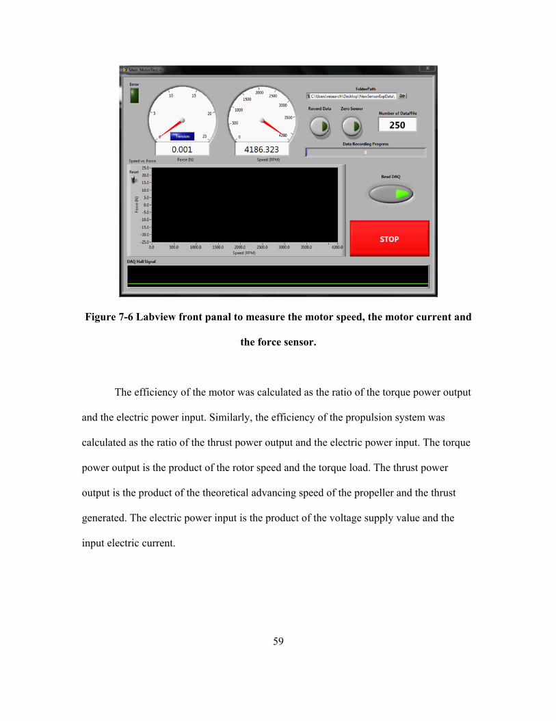
59

Figure 7-6 Labview front panal to measure the motor speed, the motor current and

the force sensor.

The efficiency of the motor was calculated as the ratio of the torque power output

and the electric power input. Similarly, the efficiency of the propulsion system was

calculated as the ratio of the thrust power output and the electric power input. The torque

power output is the product of the rotor speed and the torque load. The thrust power

output is the product of the theoretical advancing speed of the propeller and the thrust

generated. The electric power input is the product of the voltage supply value and the

input electric current.

60

7.5. Results and discussion

The experiment was completed to determine the performance of the propulsion

system. The brushless DC motor was insulated using the 3D printed housing and sealed

properly to ensure no water leakage into the pressure housing. The ring-propellers were

tested to measure input electric current, rotor speed, thrust and torque. The thrust FT was

plotted against the quantity 2 . Sixteen propeller with different blades number and twist

angles were tested in water. The thrust and torque of each propeller was measured.

Figure 7-7 and Figure 7-8 show the measured thrust vs. the measure propeller speed

squared for some propellers. Figure 7-9 shows the measured torque vs. the propeller

measured propeller speed squared for one of the extended blades propellers.

Figure 7-7 Thrust experiemtnal resuts of a non-extended ring thruster with 5 blades

and 120o twist angle.

61

Figure 7-8 Therust experiemtnal resuts of an extended ring thruster with 4 blades


Figure 7-9 Torque experiemtnal resuts of an extended ring thruster with 4 blades


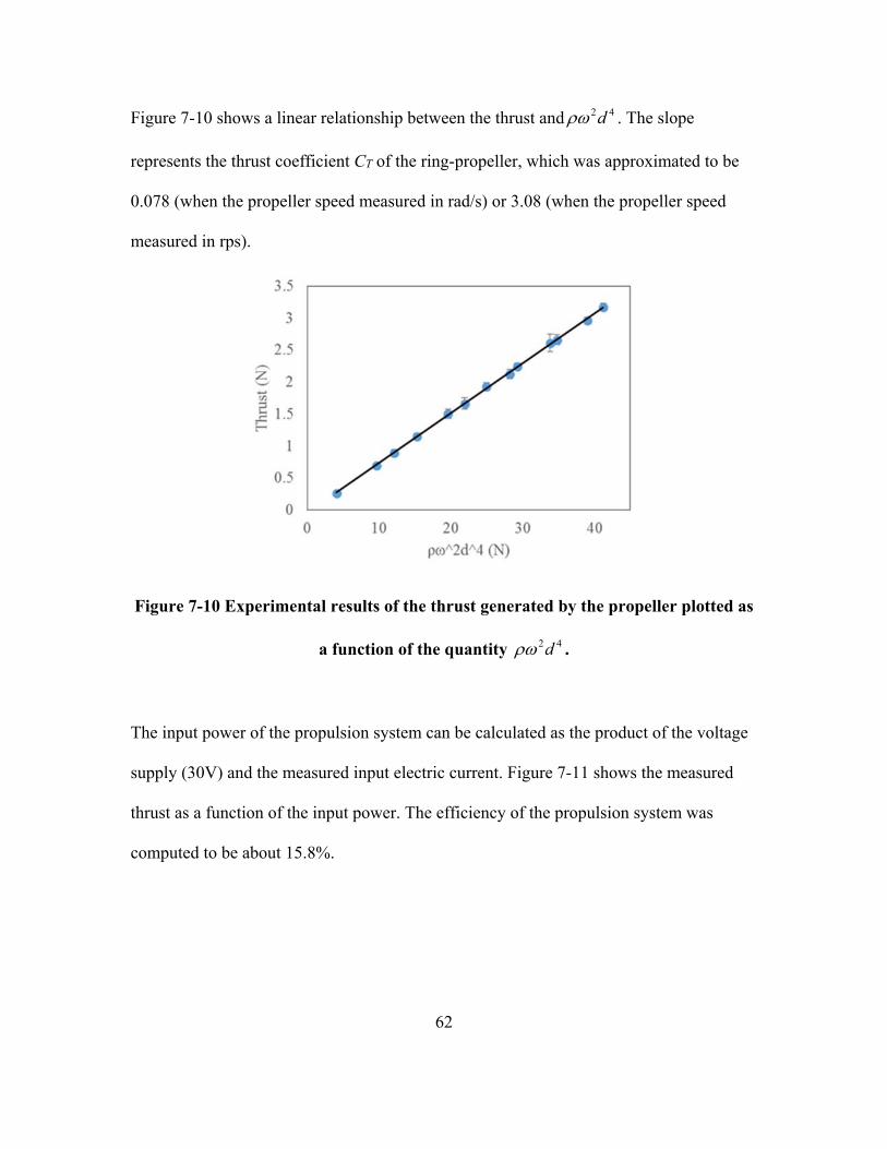
62

Figure 7-10 shows a linear relationship between the thrust and 42d . The slope

represents the thrust coefficient CT of the ring-propeller, which was approximated to be

0.078 (when the propeller speed measured in rad/s) or 3.08 (when the propeller speed

measured in rps).

Figure 7-10 Experimental results of the thrust generated by the propeller plotted as

a function of the quantity 42d .

The input power of the propulsion system can be calculated as the product of the voltage

supply (30V) and the measured input electric current. Figure 7-11 shows the measured

thrust as a function of the input power. The efficiency of the propulsion system was

computed to be about 15.8%.

63

Figure 7-11 Experimental results of the propulsion system thrust as a function of the

input power.

Figure 7-12 is the experimental results of the ring-propeller torque plotted as a

function of the quantity 52d . The relationship between the two quantities should be

linear. However, the measured torque was low and associated with a lot of vibrations and

disturbance. The disturbance was due to the water movement against the structured stand.

The torque constant was approximated to be 0.098 (when the propeller speed measured in

rad/s) or 3.86 (when the propeller speed measured in rps). Figure 7-13 shows the

measured torque as a function of the input power. The efficiency of the motor at the

operating point is 46.84% which conclude that the ring propeller efficiency to be 33.71%.

64

Figure 7-12 Experimental results of the ring-propeller torque as a function of the

quantity 52d .

Figure 7-13 Experimental results of the propulsion system Torque as a function of

the input power.

65

8. CONTROLLER DESIGN

Two systems require controller designs. First, the propulsion system that runs by the

three-phase DC brushless motor. Second, mUV motion system, which represents the

aerodynamics of the vehicle.

8.1. Motor controller

The three-phase DC brushless motor requires an electronics speed controller (ESC). The

system (the motor) has three electric currents as inputs and rotor rotational speed as an

output. The position sensors can detect the rotor speed as a feedback to the closed loop

(see Figure 8-1)

Figure 8-1 Block diagram of the motor system showing a negative feedback control.

Hall Effect sensor where used to measure the rotor speed as a negative feedback

to close the loop of the motor using a commercially available controller. The Anaheim

Controller (Electrical Commutator, Figure 8-2) produces the necessary electrical currents

to rotate the motor at a desired speed.

66

Figure 8-2 Anaheim Automation Brushless Speed Controller board mount with

connection diagram.

8.2. Vehicle controller stability

The motor is controlled by the Anaheim controller with a negative closed loop feedback.

This subsystem is stable and operates independently. Therefore, the ODE equation (4.16)

can be reduced by eliminating x2 and converted it to an input ( 223 xxu ) to the new

system as it shown in equation (8.1).

4351416

4351415

34

211313313

31111121

cossin

sincos

xxaxxx

xxaxxVx

xx

uxxbxax

uaxxax

ox

(8.1)

67

Similar concept can be applied to the mUV velocity (x1) and the mUV yaw speed

(x3). Lyapunov stability analysis was performed on this nonlinear dynamic subsystem

with zero inputs. Choosing V(x) to be 23

2121 xx , the V (x) can be described as

023311

2112 xaxxaV which is always negative for nonzero x1 and x3 because the

constants coefficients are physical positive values.

8.3. Electric circuit and communications

The propulsion generator has several sub-components such as motor-thruster, motor-

controller, and motherboard, PWM-DC converter, batteries and receiver (see Figure 8-3).

The motherboard circuit (PCB) was designed with Eagle CAD software (Figure 8-4) to

interface with the motor, motor controller, PWM-DC converters, receiver and battery

back (see Figure 8-5).

Figure 8-3 Propulsion generator schematics.

68

Figure 8-4 Motherboard circuit design using Eagle CAD.

Figure 8-5 Propulsion system electronic ciruit board.

The motor can be controlled wirelessly by an open loop remote controller with

three inputs (throttles). The throttles control the power Enable/Disable option, rotor

rotation direction (clockwise or counter clockwise) and the rotor speed.

69

9. CONCOLUSION AND FUTURE WORK

9.1. Conclusion

The major findings and contributions of my thesis are:

1) The underwater vehicle structure was defined to have a torpedo shape with a

through-hole (same size of the ring propeller) that permits water flow from the

front to the rear. The length of the vehicle was decided to be twice as much the

frontal diameter. Therefore, the total volume of the vehicle was constraint with

two variables such as the frontal diameter and the ring-propeller diameter. The

onboard energy density was taking in to the account along with the vehicle-

desired performance to be integrated as constraints to minimize the underwater

vehicle outer diameter. Those constraints determined how far the underwater

vehicle frontal diameter could be pushed to the minimum without dropping the

vehicle performance. It turns out that the smallest underwater vehicle with the

specified shape and desired performance to be 6 inches in frontal diameter and 1.6

inches in ring propeller diameter.

2) The size of the miniaturized underwater vehicle was determined. The propulsion

system for such a small vehicle size, occupancy and environmental constraint

dedicate the urge of designing a custom driving motor to enable vehicle motion. A

brushless three-phase DC motor with inrunner rotor permanent magnets was

designed and fabricated to have about 3 inches outer diameter and 1.6 inches

inner diameter. The air gap diameter was 2.08 inches. The motor can operate in

water and rotate at speed of 1200 rpm with the maximum underwater load

70

providing 30 V power supply. The motor constant was determined numerically

and experimentally to be about 0.014.

3) A new technique was developed to pressure house the brushless three-phase DC

motor with inrunner rotor permanent magnets. The concept of the design was

inspired by the current existing pressure housing method with much simpler

structure. The pressure housing prevents the motor electronic circuit components

to encounter with the ambient water. A three-dimensional printed pressure

housing was built to house the stator winding and its electronics leaving the rotor

magnets and the ring propeller to be consistently exposed to water. Several tests

were performed on the housing and no leaks were found. The same technique can

be modified to enable proper functionality in the seep-sea. An aluminum housing

with oil filling will be required to enable deep-sea compatibility.

4) Several types of ring propellers were designed and three-dimensionally printed.

Each propeller was designed using blade element theory, which maximizes thrust

and efficiency depending on the operating point. A structure with force sensor

was built to examine each the brushless three-phase DC motor with each ring

propeller. The ring propellers were different in terms of number of blades, pitch

or twist angle and blade extensions. After many experiments and testes, I

concluded that the ring-propeller with extended three blades and 60o twist angle

was the best. The maximum thrust generated was about 3.25 N with a propeller

efficiency of 0.46.

71

9.2. Future work

Although my research built a solid foundation for developing a miniaturized underwater

vehicle, still other problems need to be solved before deploying it to the field. For

instance, fins are needed to allow vehicle motion in all directions. In addition, a

communication method is required to enable vehicle remote controlling. Since the vehicle

is designed to carry underwater device measurements, additional communication

technique and power sourcing is required which might influence the vehicle overall size

and performance. Other future work involve upgrading the vehicle to function in the

deep-sea using the proposed pressure housing technique. This constructed pressure

housing will function in the deep-sea in order to resist pressures found by ranging up to

3000m deep in the ocean. Finally, design several miniaturized underwater vehicle and

enable communication among themselves to perform simultaneously and efficiently to

perform a task. For example, several miniaturized underwater vehicles can swim and

form node simultaneous measurements.

72

REFERENCES

Allen, B., Stokey, R., Austin, T., Forrester, N., Goldsborough, R., Purcell, M., & von Alt, C. (1997, October). REMUS: a small, low cost AUV; system description, field trials and performance results. In OCEANS'97. MTS/IEEE Conference Proceedings (Vol. 2, pp. 994-1000). IEEE.

Arafat, H. N., Stilwell, D. J., & Neu, W. L. (2006). Development of a dynamic model of

a small high-speed autonomous underwater vehicle. OCEANS 2006, 1-6. Atallah, K., Zhu, Z. Q., & Howe, D. (1992). An improved method for predicting iron

losses in brushless permanent magnet DC drives. Magnetics, IEEE Transactions on, 28(5), 2997-2999.

Alvarez, A., Caffaz, A., Caiti, A., Casalino, G., Gualdesi, L., Turetta, A., & Viviani, R.

(2009). Folaga: A low-cost autonomous underwater vehicle combining glider and AUV capabilities. Ocean Engineering, 36(1), 24-38.

Behar, A. E., Bruhn, F. C., & Carsey, F. (2003). Exploring miniaturization limits for an

instrumented autonomous submersible explorer for extreme environments. 13th International Symposium on Unmanned Untethered Submersible Technology,

Bellingham, J. G., Zhang, Y., Kerwin, J. E., Erikson, J., Hobson, B., Kieft, B., . . . Paul, J.

(2010). Efficient propulsion for the tethys long-range autonomous underwater vehicle. Autonomous Underwater Vehicles (AUV), 2010 IEEE/OES, 1-7.

Bradley, A., Duester, A., Liberatore, S., & Yoerger, D. (2000). Extending the endurance

of an operational scientific AUV using lithium-ion batteries. Proceedings of UUVS, Bradshaw, A., Hamacher, T., & Fischer, U. (2011). Is nuclear fusion a sustainable energy

form? Fusion Engineering and Design, 86(9), 2770-2773. Briggs, R. C. (2010). Mechanical Design of a Self-Mooring Autonomous Underwater

Vehicle, Brown Jr, O., & Hendrick, H. (1986). ROBOTIC VEHICLES: A REVIEW. Human

Factors in Organizational Design and Management-II: Proceedings of the Second Symposium Held in Vancouver, BC, Canada, 19-21 August, 1986, , 2 29.

Chalk, S. G., & Miller, J. F. (2006). Key challenges and recent progress in batteries, fuel

cells, and hydrogen storage for clean energy systems. Journal of Power Sources, 159(1), 73-80.

73

Davis, R. E., Eriksen, C. C., & Jones, C. P. (2002). Autonomous buoyancy-driven underwater gliders. The Technology and Applications of Autonomous Underwater Vehicles, , 37-58.

deYoung, B., Heath, M., Werner, F., Chai, F., Megrey, B., & Monfray, P. (2004).

Challenges of modeling ocean basin ecosystems. Science (New York, N.Y.), 304(5676), 1463-1466. doi:10.1126/science.1094858 [doi]

Dickey, T. D. (1991). The emergence of concurrent high‐resolution physical and bio‐

optical measurements in the upper ocean and their applications. Reviews of Geophysics, 29(3), 383-413.

Donovan, G. T. (2012). Position error correction for an autonomous underwater vehicle

inertial navigation system (INS) using a particle filter. Oceanic Engineering, IEEE Journal of, 37(3), 431-445.

Ekinci, S. (2011). A practical approach for design of marine propellers with systematic

propeller series. Brodogradnja, 62(2), 123-129. Eriksen, C. C., Osse, T. J., Light, R. D., Wen, T., Lehman, T. W., Sabin, P. L., . . .

Chiodi, A. M. (2001). Seaglider: A long-range autonomous underwater vehicle for oceanographic research. Oceanic Engineering, IEEE Journal of, 26(4), 424-436.

Gage, J. D., & Tyler, P. A. (1992). Deep-sea biology: A natural history of organisms at

the deep-sea floor Cambridge University Press. Gracias, N., & Santos-Victor, J. (2000). Underwater video mosaics as visual navigation

maps. Computer Vision and Image Understanding, 79(1), 66-91. Greig, J., & Sathirakul, K. (1961). Pole-face losses in alternators. an investigation of

eddy-current losses in laminated pole shoes. Proceedings of the IEE-Part C: Monographs, 108(13), 130-138.

Gundogdu, T., & Komurgoz, G. (2010). Design of permanent magnet machines with

different rotor type. World Academy of Science, Engineering and Technology, 70 Healey, A. J., Rock, S. M., Cody, S., Miles, D., & Brown, J. P. (1995). Toward an

improved understanding of thruster dynamics for underwater vehicles. Oceanic Engineering, IEEE Journal of, 20(4), 354-361.

Holik, P. J., Dorrell, D. G., Lombard, P., Thougaard, H., & Jensen, F. (2006). A multi-

sliced finite element model for induction machines incorporating inter-bar current. Industry Applications Conference, 2006. 41st IAS Annual Meeting. Conference Record of the 2006 IEEE, , 2 819-826.

74

Huang, C., Yang, T., Liu, J., & Schindall, J. (2013). Acoustic mapping of ocean currents using networked distributed sensors. The Journal of the Acoustical Society of America, 134(3), 2090-2105.

Hyakudome, T., Yoshida, H., Ishibashi, S., Sawa, T., & Nakamura, M. (2011).

Development of advanced lithium-ion battery for underwater vehicle. Underwater Technology (UT), 2011 IEEE Symposium on and 2011 Workshop on Scientific use of Submarine Cables and Related Technologies (SSC), 1-4.

Hyakudome, T. (2011). Design of autonomous underwater vehicle. International Journal

of Advanced Robotic Systems, 8(1) Isern, A., & Clark, H. (2003). The ocean observatories initiative: A continued presence

for interactive ocean research. Marine Technology Society Journal, 37(3), 26-41. Islam, R., Husain, I., Fardoun, A., & McLaughlin, K. (2009). Permanent-magnet

synchronous motor magnet designs with skewing for torque ripple and cogging torque reduction. Industry Applications, IEEE Transactions on, 45(1), 152-160.

Jahnke, R. A., & Christiansen, M. B. (1989). A free-vehicle benthic chamber instrument

for sea floor studies. Deep Sea Research Part A. Oceanographic Research Papers, 36(4), 625-637.

Karl, T. R., & Trenberth, K. E. (2003). Modern global climate change. Science (New

York, N.Y.), 302(5651), 1719-1723. doi:10.1126/science.1090228 [doi] Kennedy, G. C., & Holt, J. K. (1995). Developing a high efficiency means of propulsion

for underwater vehicles. Southcon/95. Conference Record, 352-356. Kim, S., Choi, H., Lee, J., & jun Lee, Y. (2014). Design, implementation, and experiment

of an underwater robot for effective inspection of underwater structures. Robot intelligence technology and applications 2 (pp. 821-829) Springer.

Korgen, B. J., Bodvarsson, G., & Kulm, L. (1970). Current speeds near the ocean floor

west of oregon. Deep Sea Research and Oceanographic Abstracts, , 17(2) 353-357. Koss, M., Booth, T., & Sullo, K.On the measurement of the characteristic rotation decay

time for a baseball. Larsen, M. B. (2000). Synthetic long baseline navigation of underwater vehicles.

OCEANS 2000 MTS/IEEE Conference and Exhibition, , 3 2043-2050. Lloret, J., Sendra, S., Ardid, M., & Rodrigues, J. J. (2012). Underwater wireless sensor

communications in the 2.4 ghz ism frequency band. Sensors, 12(4), 4237-4264.

75

Lopez-de-Heredia, A., Calleja, C., Lertxundi, A., Aranburu, A., & Nieva, T. (2011). Stator current and power factor optimization in an IPMSM for railway traction application. Power Electronics and Applications (EPE 2011), Proceedings of the 2011-14th European Conference on, 1-10.

Maier-Reimer, E., & Hasselmann, K. (1987). Transport and storage of CO2 in the

ocean——an inorganic ocean-circulation carbon cycle model. Climate Dynamics, 2(2), 63-90.

Manwel, J., McGowan, J., & Rogers, A. (2002). Wind energy explained. Martin, S. C., Whitcomb, L. L., Yoerger, D., & Singh, H. (2006). A mission controller

for high level control of autonomous and semi-autonomous underwater vehicles. OCEANS 2006, 1-6.

Matuszewski, L., & Falkowski, K. (2003). Ring thruster with magnetic bearings.

OCEANS 2003. Proceedings, , 4 2023-2031. Mavor, J. W., Froehlich, H. E., Marquet, W. M., & Rainnie, W. O. (1967). Alvin, 6000-ft.

submergence research vehicle Woods Hole Oceanographic Institution. Murakami, H., Kataoka, H., Honda, Y., Morimoto, S., & Takeda, Y. (2001). Highly

efficient brushless motor design for an air-conditioner of the next generation 42 V vehicle. Industry Applications Conference, 2001. Thirty-Sixth IAS Annual Meeting. Conference Record of the 2001 IEEE, , 1 461-466.

Okamoto, M., Yasuda, K., & Azuma, A. (1996). Aerodynamic characteristics of the

wings and body of a dragonfly. The Journal of Experimental Biology, 199(Pt 2), 281-294.

Petrich, J., & Stilwell, D. J. (2011). Robust control for an autonomous underwater vehicle

that suppresses pitch and yaw coupling. Ocean Engineering, 38(1), 197-204. Pivano, L., Johansen, T., Smogeli, O., & Fossen, T. (2007). Nonlinear thrust controller

for marine propellers in four-quadrant operations. American Control Conference, 2007. ACC'07, 900-905.

Poole, P. K., & Clower, P. (1996). A systems approach to autonomous underwater

vehicle (AUV) propulsion design. Marine Technology Society Journal, 30(2), 8-16. Post, R. S. (1999). Permanent magnet coupling fundamentals. AISE steel technology, 76,

54-58. Prestero, T. T. J. (2001). Verification of a Six-Degree of Freedom Simulation Model for

the REMUS Autonomous Underwater Vehicle,

76

Ramírez, J. A., Vásquez, R. E., Gutiérrez, L. B., & Flórez, D. A. (2007).

Mechanical/Naval design of an underwater remotely operated vehicle (ROV) for surveillance and inspection of port facilities. ASME 2007 International Mechanical Engineering Congress and Exposition, 351-361.

Rowe, F., & Young, J. (1979). An ocean current profiler using doppler sonar.

OCEANS'79, 292-297. Ruiz, S., Garau, B., Martínez-Ledesma, M., Casas, B., Pascual, A., Vizoso, G., . . .

Testor, P. (2012). New technologies for marine research: 5 years of glider activities at IMEDEA-TMOOS. Scientia Marina, 76(S1), 261-270.

Sasdelli, K. R., & Spargo, J. D. (1971). Rotary Shaft Seal Selection Handbook for

Pressure-Equalized, Deep-Ocean Equipment (No. NSRDL/A-7-573). NAVAL SHIP RESEARCH AND DEVELOPMENT LABANNAPOLIS MD.

Schelleng, J., Burrows, C., & Ferrell, E. (1933). Ultra-short-wave propagation. Radio

Engineers, Proceedings of the Institute of, 21(3), 427-463. Schubel, P. J., & Crossley, R. J. (2012). Wind turbine blade design. Energies, 5(9), 3425-

3449. Shaneyfelt, T., Joordens, M. A., Nagothu, K., & Jamshidi, M. (2008). RF communication

between surface and underwater robotic swarms. WAC'08: Proceedings of the World Automation Congress' 08, 1-6.

Sharkh, S. A., Lai, S. H., & Turnock, S. (2004). Structurally integrated brushless PM

motor for miniature propeller thrusters. IEE Proceedings-Electric Power Applications, 151(5), 513-519.

Shen, Q., Wang, T., Liang, J., & Wen, L. (2013). Hydrodynamic performance of a

biomimetic robotic swimmer actuated by ionic polymer–metal composite. Smart Materials and Structures, 22(7), 075035.

Singh, H., Yoerger, D., & Bradley, A. (1997). Issues in AUV design and deployment for

oceanographic research. Robotics and Automation, 1997. Proceedings., 1997 IEEE International Conference on, , 3 1857-1862.

Stamenkovic, I., Milivojevic, N., Schofield, N., Krishnamurthy, M., & Emadi, A. (2013).

Design, analysis, and optimization of ironless stator permanent magnet machines. Power Electronics, IEEE Transactions on, 28(5), 2527-2538.

Takeuchi, J., Miraghaie, R., Yuki, K., Satake, S., Kunugi, T., & Morley, N. (2003).

Turbulent velocity profile measurement in circular pipe flow using particle image

77

velocimetry technique. Fusion Engineering, 2003. 20th IEEE/NPSS Symposium on, 140-143.

Tivey, M. A., & Johnson, H. P. (1990). The magnetic structure of axial seamount, juan de

fuca ridge. Journal of Geophysical Research: Solid Earth (1978–2012), 95(B8), 12735-12750.

Tonder, K., & Salant, R. (1992). Non-leaking lip seals: a roughness effect study.Journal

of tribology, 114(3), 595-599. Tunnicliffe, V. (1992). Hydrothermal-vent communities of the deep sea. American

Scientist, , 336-349. Tyson, F. L., Rice, D. L., & Dearry, A. (2004). Connecting the oceans and human health.

Environmental Health Perspectives, 112(8), A455-6. Vasilescu, I., Varshavskaya, P., Kotay, K., & Rus, D. (2005). Autonomous modular

optical underwater robot (amour) design, prototype and feasibility study. Robotics and Automation, 2005. ICRA 2005. Proceedings of the 2005 IEEE International Conference on, 1603-1609.

von Alt, C. (2003). Autonomous underwater vehicles. Autonomous Underwater

Lagrangian Platforms and Sensors Workshop, , 3 Watson, S. A., & Green, P. N. (2010). Propulsion systems for micro-autonomous

underwater vehicles (μAUVs). Robotics Automation and Mechatronics (RAM), 2010 IEEE Conference on, 435-440.

Winter, M., & Brodd, R. J. (2004). What are batteries, fuel cells, and supercapacitors?

Chemical Reviews, 104(10), 4245-4270. Witze, A. (2013). Marine science: Oceanography's billion-dollar baby. Nature,

501(7468), 480-482. doi:10.1038/501480a [doi] Yakovlev, A. Y., Sokolov, M. A., & Marinich, N. V. (2011). Numerical design and

experimental verification of a RIM-driven thruster. Proceedings of Second International Symposium on Marine Propulsors. Hamburg, Germany,

Yang, Z., Zhang, J., Kintner-Meyer, M. C., Lu, X., Choi, D., Lemmon, J. P., & Liu, J.

(2011). Electrochemical energy storage for green grid. Chemical Reviews, 111(5), 3577-3613.

Yeadon, W. H., & Yeadon, A. W. (Eds.). (2001). HB SMALL ELECTRIC MOTORS, 1.

McGraw Hill Professional.

78

Yildiz, O., Yilmaz, A. E., & Gokalp, B. (2009). State-of-the-art system solutions for unmanned underwater vehicles. Sensors, 1, 2.

Yoerger, D. R., Jakuba, M., Bradley, A. M., & Bingham, B. (2007). Techniques for deep

sea near bottom survey using an autonomous underwater vehicle. The International Journal of Robotics Research, 26(1), 41-54.

Yoerger, D. R., & Newman, J. B. (1986). Jason: An integrated approach to rov and

control system design. ROV’86: Remotely operated vehicles (pp. 340-353) Springer. Yoerger, D. R., Newman, J., & Slotine, J. (1986). Supervisory control system for the

jason rov. Oceanic Engineering, IEEE Journal of, 11(3), 392-400. Yoerger, D. R., Von Alt, C. J., Bowen, A. D., & Newman, J. (1986). Design of

underwater vehicles for high performance control. OCEANS'86, 1431-1437. Yoerger, D., Bradley, A., Martin, S., & Whitcomb, L. (2006). The sentry autonomous

underwater vehicle: Field trial results and future capabilities. AGU Fall Meeting Abstracts, , 1 1674.

Yuh, J. (2000). Design and control of autonomous underwater robots: A survey.

Autonomous Robots, 8(1), 7-24. Yuh, J., Choi, S., Ikehara, C., Kim, G., McMurty, G., Ghasemi-Nejhad, M., . . . Sugihara,

K. (1998). Design of a semi-autonomous underwater vehicle for intervention missions (SAUVIM). Underwater Technology, 1998. Proceedings of the 1998 International Symposium on, 63-68.

79

APPENDIX A

mUV OPTIMAL MOTION TRAJECTORY

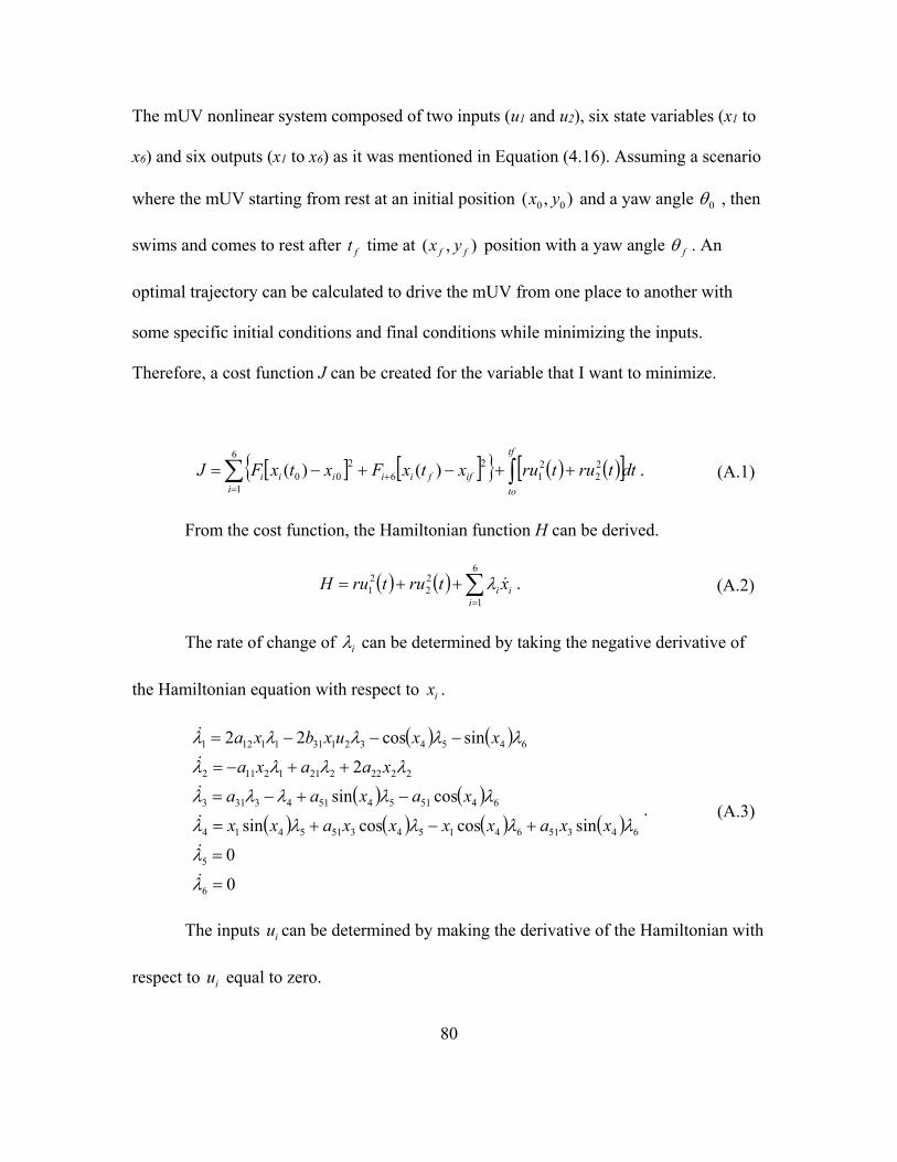
80

The mUV nonlinear system composed of two inputs (u1 and u2), six state variables (x1 to

x6) and six outputs (x1 to x6) as it was mentioned in Equation (4.16). Assuming a scenario

where the mUV starting from rest at an initial position ),( 00 yx and a yaw angle 0 , then

swims and comes to rest after ft time at ),( ff yx position with a yaw angle f . An

optimal trajectory can be calculated to drive the mUV from one place to another with

some specific initial conditions and final conditions while minimizing the inputs.

Therefore, a cost function J can be created for the variable that I want to minimize.

dttrutruxtxFxtxFJtf

toiiffiiiii

22

21

6

1

26

200 )()( . (A.1)

From the cost function, the Hamiltonian function H can be derived.

6

1

22

21

iii xtrutruH . (A.2)

The rate of change of i can be determined by taking the negative derivative of

the Hamiltonian equation with respect to ix .

0

0

sincoscossin

cossin

2

sincos22

6

5

64351641543515414

6451545143313

222222112112

64543213111121

xxaxxxxaxx

xaxaa

xaaxa

xxuxbxa

. (A.3)

The inputs iu can be determined by making the derivative of the Hamiltonian with

respect to iu equal to zero.

81

02

02

311312

2211

xxbru

bru. (A.4)

The ODEs described in equations (4.16), (A.3) and (A.4) can be used to solve for

the necessary inputs iu .

A MATLAB code was generated to solve the optimal trajectory problem with the

initial and final conditions described in Table A–1. The code solves the ODE sets by

iteration going from forward and backward in time.

Table A–1

Optimal trajectory example initial and final conditions

Variable Initial time (0 sec) Final time (300 sec)

mUV speed ( 1x ) 0 0

Propeller speed ( 2x ) 0 0

mUV yaw speed ( 3x ) 0 0

mUV yaw angle ( 4x ) 0o 0o

mUV x location ( 5x ) 0 80 m

mUV y location ( 6x ) 0 50 m

After about 400 iterations (18 hours), the solution converges with an error near

10-5 (see Figure A-1).

82

Figure A-1 MATLAB results of the optimal trajectory example of the mUV going

from initial position to the final position in 300 sec.

The MATLAB code is composed of three .m files.

ODE_L.m MATLAB file

function dL = ODE_L(t,L,tu,x,u,A,B)

a11 = A(1);

a12 = A(2);

a21 = A(3);

a22 = A(4);

a31 = A(5);

a51 = A(6);

b21 = B(1);

0 50 100 150 200 250 3000

0.5mUV Speed

0 50 100 150 200 250 3000

2040

Prop Speed

0 50 100 150 200 250 300

-0.020

0.02

Yaw Speed

0 50 100 150 200 250 3000

20

40Yaw Angle

0 50 100 150 200 250 3000

50

X

0 50 100 150 200 250 3000

50Y

0 10 20 30 40 50 60 70 800

10

20

30

40

50

XError = 9.9539e-005 # Cycle = 621

Y

0 50 100 150 200 250 3000

1

2Motor Current

0 50 100 150 200 250 300-2

0

2x 10

-3 Angle Ref

Time (sec)

83

b31 = B(2);

u(1) = spline(tu,u(:,1),t);


x(1) = spline(tu,x(:,1),t);






dL = zeros(6,1);

dL(1) = 2*a12*x(1)*L(1) + 2*b31*x(1)*u(2)*L(3) - L(5)*cos(x(4)) - L(6)*sin(x(4));

dL(2) = -2*a11*x(2)*L(1) + a21*L(2) + 2*a22*x(2)*L(2);

dL(3) = a31*L(3) - L(4) + a51*sin(x(4))*L(5) - a51*cos(x(4))*L(6);

dL(4) = x(1)*L(5)*sin(x(4)) - x(1)*L(6)*cos(x(4)) + a51*x(3)*cos(x(4))*L(5) +

a51*x(3)*sin(x(4))*L(6);

dL(5) = 0;

dL(6) = 0;

ODE_x.m MATLAB file

function dx = ODE_x(t,x,tu,u,A,B) a11 = A(1); a12 = A(2);

a21 = A(3);

84

a22 = A(4);

a31 = A(5);

a51 = A(6);

b21 = B(1);

b31 = B(2);



dx = zeros(6,1);

dx(1) = a11*x(2)*abs(x(2)) - a12*x(1)*abs(x(1));

dx(2) = - a21*x(2) - a22*x(2)*abs(x(2)) + b21*u(1);

dx(3) = - a31*x(3) - b31*x(2)*abs(x(2))*u(2);

dx(4) = x(3);

dx(5) = x(1)*cos(x(4)) - a51*x(3)*sin(x(4));

dx(6) = x(1)*sin(x(4)) + a51*x(3)*cos(x(4));

Solver.m MATLAB file

clear;clc;close all

GetU;

S = figure(1);

set(S,'Position',[50 60 1200 600]);

rho = 1000;

Cd = 0.267;

85

m = 3.77;

A = pi*(3*.0254)^2;

p = .0082;

b = 1.42e-4;

N = 0.0232;

J = 0.00011538;

Ct = 0.0771;

Cq = 0.0797;

d = 1.625*.0254;

l = .5;

k = .0245;

a11 = Ct*rho*d^4/m;

a12 = rho*Cd*A/(2*m);

a21 = b/J;

a22 = Cq*rho*d^5/J;

b21 = k/J;

a31 = l/N;

b31 = p/N;

a51 = 5*.0254;

A = [a11 a12 a21 a22 a31 a51];

B = [b21 b31];

tu = linspace(t0,tf,M);

86

u(:,1) = -4.2/tf^2*tu.^2+4.2/tf*tu;

u(:,2) = zeros(M,1);

x0 = [0 0 0 theta0 x0 y0];

ER = 1e-20;

err = 1;

w = 5;

I = 1;

while err>ER

[TX,X] = ode23s(@(t,x) ODE_x(t,x,tu,u,A,B),[t0 tf],x0);

XX(:,1) = spline(TX,X(:,1),tu);






Lambda1tf = F1*(XX(end,1));



Lambda4tf = F4*(XX(end,4)-thetaf);

Lambda5tf = F5*(XX(end,5)-xf);

Lambda6tf = F6*(XX(end,6)-yf);

clear U

87

U(:,1) = spline(tu',u(:,1),TX);

U(:,2) = spline(tu',u(:,2),TX);

[TL,Lam] = ode23s(@(t,L) ODE_L(t,L,TX,X,U,A,B),[tf t0],[Lambda1tf Lambda2tf

Lambda3tf Lambda4tf Lambda5tf Lambda6tf]);

Lambda(:,1) = spline(TL,Lam(:,1),tu);






dHdu1 = 2*r1*u(:,1) + b21*Lambda(:,2);

dHdu2 = 2*r2*u(:,2) - b31*Lambda(:,3).*XX(:,2).*abs(XX(:,2));

u1_new = u(:,1) - EPS*dHdu1;

u2_new = u(:,2) - EPS*dHdu2;

err = max(abs(u(:,1)-u1_new))+max(abs(u(:,2)-u2_new));

u(:,1) = u1_new;

u(:,2) = u2_new;

if w >= 0

subplot(5,2,1)

plot(tu,XX(:,1))

title('mUV Speed')

subplot(5,2,2)

88

plot(tu,XX(:,2))

title('Prop Speed')

subplot(5,2,3)

plot(tu,XX(:,3))

title('Yaw Speed')

subplot(5,2,4)

plot(tu,XX(:,4)*180/pi)

title('Yaw Angle')

subplot(5,2,5)

plot(tu,XX(:,5))

title('X')

subplot(5,2,6)

plot(tu,XX(:,6))

title('Y')

subplot(5,2,[7,9])

plot(XX(:,5),XX(:,6))

xlabel('X';['Error = ' num2str(err) ' # Cycle = ' num2str(I)])

ylabel('Y')

subplot(5,2,8)

plot(tu,u(:,1))

title('Motor Current')

subplot(5,2,10)

89

plot(tu,u(:,2))

title('Angle Ref')

drawnow

w = 0;

I = I + 1;

end

w = w + 1;

end

GetU.m MATLAB file

F1 = 1000000;

F2 = 10;

F3 = 1;

F4 = 10000;

F5 = 50; %X

F6 = 30; %Y

r1 = 1;

r2 = 0.001;

M = 80;

EPS = 1e-10;

t0 = 0;

tf = 300;

90

x0 = 0;

y0 = 0;

xf = 80;

yf = 50;

theta0 = 10*pi/180;

thetaf = 50*pi/180;

91

APPENDIX B

FRONTAL DRAG OF THE mUV

92

The drag coefficient CD of the vehicle can be calculated using the drag force equation.

In a laminar flow, the drag coefficient can depend only on the Reynolds's Number Re;

wind tunnel test is usually the comment method to determine the drag force acting on a

body exposed to a wind speed u. However, in order to match the aerodynamic property of

the simulation, the Reynolds's Number Re of the flow using water as fluid and water

speed of 1 m/s was calculated. In that laminar flow the wind, speed was determined using

the same Re and air thermodynamic properties. The wind speed is about 15.25 times

higher than the water current speed (see Figure B-2).

The experiment was performed at Arizona State University in the mechanical

engineering wind tunnel facility. The experimental data are plotted in Figure B-3, which

shows as expected a linear relation between the dynamic pressure and the drag pressure.

Figure B-2 Schematics of the experimental setup.

93

Figure B-3 Experimental Data of the AUV drag pressure vs. dynamic pressure. The

equation of the linear regression fit for this data is Pdrag = 3.75 Pdyn. The measured

frontal drag coefficient of the mUV is 0.267.

Design of Miniaturized Underwater Vehicle with Propulsions … · Design of Miniaturized Underwater...

Documents

Transcript of Design of Miniaturized Underwater Vehicle with Propulsions … · Design of Miniaturized Underwater...