
DESIGN OF HIGH EFFICIENCY BLOWERS FOR FUTURE AEROSOL … · 2017-10-14 · DESIGN OF HIGH...
123
DESIGN OF HIGH EFFICIENCY BLOWERS FOR FUTURE AEROSOL APPLICATIONS A Thesis by RAMAN CHADHA Submitted to the Office of Graduate Studies of Texas A&M University in partial fulfillment of the requirements for the degree of MASTER OF SCIENCE December 2005 Major Subject: Mechanical Engineering
Transcript of DESIGN OF HIGH EFFICIENCY BLOWERS FOR FUTURE AEROSOL … · 2017-10-14 · DESIGN OF HIGH...

DESIGN OF HIGH EFFICIENCY BLOWERS FOR FUTURE
AEROSOL APPLICATIONS
A Thesis
by
RAMAN CHADHA
Submitted to the Office of Graduate Studies of
Texas A&M University
in partial fulfillment of the requirements for the degree of
MASTER OF SCIENCE
December 2005
Major Subject: Mechanical Engineering

DESIGN OF HIGH EFFICIENCY BLOWERS FOR FUTURE
AERSOSOL APPLICATIONS
A Thesis
by
RAMAN CHADHA
Submitted to the Office of Graduate Studies of
Texas A&M University
in partial fulfillment of the requirements for the degree of
MASTER OF SCIENCE
Approved by:
Chair of Committee, Gerald L. Morrison
Committee Members, Andrew R. McFarland
Yassin A. Hassan
John Haglund
Head of Department, Dennis O’Neal
December 2005
Major Subject: Mechanical Engineering

iii
ABSTRACT
Design of High Efficiency Blowers for
Future Aerosol Applications. (December 2005)
Raman Chadha, B-En., IIT-Kanpur, India
Chair of Advisory Committee: Dr. Gerald Morrison
High efficiency air blowers to meet future portable aerosol sampling applications were
designed, fabricated, and evaluated. A Centrifugal blower was designed to achieve a flow
rate of 100 L/min ( )/sm 1067.1 33−× and a pressure rise of WC"4 ( )Pa 1000 . Commercial
computational fluid dynamics (CFD) software, FLUENT 6.1.22, was used extensively
throughout the entire design cycle. The machine, Reynolds number ( )Re , was around 510
suggesting a turbulent flow field. Renormalization Group (RNG) εκ − turbulent model
was used for FLUENT simulations. An existing design was scaled down to meet the
design needs. Characteristic curves showing static pressure rise as a function of flow rate
through the impeller were generated using FLUENT and these were validated through
experiments.
Experimentally measured efficiency ( )EXPη for the base-design was around 10%. This
was attributed to the low efficiency of the D.C. motor used. CFD simulations, using the
εκ − turbulent model and standard wall function approach, over-predicted the pressure
rise values and the percentage error was large.
Enhanced wall function under-predicted the pressure rise but gave better agreement (less
than 6% error) with experimental results. CFD predicted a blower scaled 70% in planar
direction ( )XZ and 28% in axial direction ( )Y and running at 19200 rpm
([email protected]) as the most appropriate choice. The pressure rise is 1021 Pa at the

iv
design flow rate of 100 L/min. FLUENT predicts an efficiency value based on static head
( )FLUη as 53.3%. Efficiency value based on measured static pressure rise value and the
electrical energy input to the motor ( )EXPη is 27.4%. This is almost a 2X improvement
over the value that one gets with the hand held vacuum system blower.

v
DEDICATION
This work is the outcome of the unconditional love and support that my parents, Mrs.
Suchita Chadha and Mr. Vijay Kumar Chadha, have for me. Their blessings,
encouragement, and the ability to see the good in me and believe in me – even when I
had doubts about myself, have brought me to the present stage.
Finally, every deed of mine reminds me of a higher guiding power above: He who is
instrumental for all the change. It is at all times that I seek his blessings!

vi
ACKNOWLEDGEMENTS
I would like to express my gratitude to my advisor, Dr. Gerald L. Morrison, for the long
fruitful discussions we had in his office. His cheerful ‘Howdy!’ when you knocked on his
door always set the tone for the meetings. His patience, encouragement, and his ability to
mold you and point in the right direction, are the only reasons this work could be
completed. Everything I know about turbomachines, I have learned from him.
Thanks are due to Dr. Andrew R. McFarland, who had the vision for this project even
before I started working on it. His cheerful smile always uplifts you and raises your
performance level. His belief in me was my motivation all along. Thank you!
I would like to thank the members of my committee for their time and guidance,
especially Dr. John Haglund. Managing the whole ATL Lab but still having those ‘couple
of minutes’ whenever you needed his time was appreciated. He set the pace during the bi-
weekly meetings and provided fruitful insights all along.
Finally, thanks are due to all of the members of the ATL, for accepting me as one of
them: Ben Thein for helping me with the lab geography and whereabouts, John Vaughan
and Michael Salomon for their patience during the drafting and for generating beautiful
drawings, and Shishan, Vishnu, and Sridhar for the discussions we had on CFD. Their
knowledge about CFD and their patience in helping me understand CFD is
commendable. Thanks to Ashley, Clint, Manpreet, Ref, Rohit, Satya, Suvi, Travis, and
Youngjin for the good times we had together. Thank you all!

vii
TABLE OF CONTENTS
Page
ABSTRACT ...................................................................................................................... iii
DEDICATION.....................................................................................................................v
ACKNOWLEDGEMENTS............................................................................................... vi
TABLE OF CONTENTS ................................................................................................. vii
LIST OF TABLES.............................................................................................................. x
LIST OF FIGURES ........................................................................................................... xi
NOMENCLATURE, ABBREVIATIONS, AND UNITS............................................... xiv
INTRODUCTION ...............................................................................................................1
THEORY AND DESIGN....................................................................................................4
Establishing the System Requirements............................................................................4
Blower Type Selection ....................................................................................................6
Scaling and Similitude.....................................................................................................7
Specific Speed and Optimum Geometry .......................................................................11
Rotor Shape as a Function of Specific Speed ............................................................12
Selection of Optimum Specific Speed Values...........................................................14
Estimating Head Rise ( )totHΔ across an Impeller ........................................................15
First Law of Thermodynamics...................................................................................15
Sample Calculations for Impeller Specific Speed .........................................................17
Single Stage Impeller Calculations............................................................................18
Two Stage Impeller Calculations...............................................................................19
Size Calculation for Single Stage Centrifugal Blower ..............................................20
Single Stage Centrifugal Blower: Observations ............................................................20
Summary of Findings ....................................................................................................24
BLOWER BASE-DESIGN SELECTION ........................................................................25
Non-traditional Scaling..................................................................................................26
Design Approach ...........................................................................................................27
Probable Base Blower Designs......................................................................................28
Selection of the Hand-held Vacuum System (HVS) Blower: Justification...................30
COMPUTATIONAL FLUID DYNAMICS (CFD) ..........................................................33

viii
Page
Background....................................................................................................................33
CFD Approach...............................................................................................................34
FLUENT 6.1.22 - Introduction......................................................................................35
Blower Geometry for CFD Simulations ........................................................................36
GAMBIT Model ............................................................................................................38
GAMBIT Meshing.........................................................................................................39
FLUENT Model.............................................................................................................42
Turbulence Model......................................................................................................43
Inlet and Outlet Conditions........................................................................................43
Near-Wall Treatment .................................................................................................44
EXPERIMENTAL TEST RIG ..........................................................................................46
Flow Rate Measurement ................................................................................................47
Pressure Measurement ...................................................................................................48
Blower Drive .................................................................................................................49
RPM Measurement ........................................................................................................49
BASE-DESIGN SIMULATION AND EXPERIMENTAL DATA COMPARISON.......50
Blower Efficiency Definitions .......................................................................................50
Component Efficiencies.............................................................................................52
FLUENT and Experimental Efficiency Definition....................................................55
Hand-held Vacuum System Blower (100xz_100y) .......................................................56
Observation................................................................................................................59
FLUENT SIMULATIONS FOR DIFFERENT SCALING CASES.................................60
Fluent Data.....................................................................................................................60
Non-dimensional Study for Blower Simulation Results ...............................................63
EXPERIMENTAL VALIDATION FOR 65XZ_26Y@20K BLOWER ..........................67
Motor Selection .............................................................................................................67
Blower Manufacturing...................................................................................................68
Modified Test-rig...........................................................................................................68
Experimental Data .........................................................................................................70
Observations and Conclusions.......................................................................................73
ENHANCED WALL TREATMENT................................................................................74
Enhanced Wall Treatment FLUENT Simulations for 65xz_26y@20k Blower ............74
Conservative Efficiency Estimates for 65xz_26y@20k Blower ...................................76
Resizing of Blower Using Enhanced-wall Treatment ...................................................78

ix
Page
EXPERIMENTAL VALIDATION FOR 70XZ_28Y@20K BLOWER ..........................80
Results............................................................................................................................80
Conservative Efficiency Estimates for 70xz_28y@20k Blower ...................................82
Observations and Conclusions.......................................................................................84
FINAL BLOWER PROTOTYPE: DESIGN AND TESTING .........................................85
Prototype Design Setup: Blower 70xz_28y with inletδ = "009.0 and shroudδ = "012.0 ....85
Results............................................................................................................................86
SUMMARY AND CONCLUSIONS ................................................................................90
RECOMMENDATIONS FOR FUTURE WORK ............................................................92
REFERENCES ..................................................................................................................93
APPENDIX A....................................................................................................................96
APPENDIX B....................................................................................................................98
APPENDIX C..................................................................................................................100
APPENDIX D..................................................................................................................102
VITA................................................................................................................................104

x
LIST OF TABLES
Page
Table 1 Specific speed values and blower sizes at different rpms................................ 22
Table 2 Ratio of pressure head and theoretical velocity head for different rpm and
impeller diameter combinations...................................................................... 23
Table 3 Sample blower simulation data........................................................................ 61
Table 4 Efficiency values for different scaled blower at design flow rate. .................. 62
Table 5 Exponents for radius and blade width.............................................................. 65
Table 6 Blower efficiency estimates at design flow rate. ............................................. 76
Table 7 Static pressure values for different sized blowers at design flow rate............. 78
Table 8 Blower efficiency estimates at design flow rate . ............................................ 83
Table 9 Efficiency estimates for final prototype blower at design flow rate................ 89
Table A-1 Values chosen for mass flow calculation. ....................................................... 96
Table D-1 Sample data sheet for final prototype blower at design rpm. ........................ 103

xi
LIST OF FIGURES
Page
Figure 1 Top-down design approach framework..............................................................5
Figure 2 Cross-sections of different pumps: (a) Radial flow (b) Mixed flow (c)
Axial flow (Hydraulics Institute). .....................................................................6
Figure 3 Defining the geometry of a pump stage (Karassik et al. 2000, reprinted
with permission of McGraw-Hill). ...................................................................9
Figure 4 Optimum geometry as a function of BEP specific speed (Karassik et al.
2000, reprinted with permission of McGraw-Hill). .........................................13
Figure 5 Specific speed values for different pump designs (Hydraulics Institute).........13
Figure 6 Efficiency values for pump with different specific speeds (Karassik et al.
2000, reprinted with permission of McGraw-Hill). .........................................14
Figure 7 Energy balance across a control volume for a rotating impeller. .....................16
Figure 8 Efficiency ( )overallη of centrifugal pumps versus specific speed, size, and
shape (Anderson 1980). ...................................................................................23
Figure 9 Turbo blowers with backward curved blades (shroud removed). ....................29
Figure 10 Hand-held vacuum system centrifugal blower (a) Top-view (b) Side-view
showing the blades. ..........................................................................................29
Figure 11 Variety of common pump impeller meridional views from low to high
specific speeds (a – f) and with inducer (g). ....................................................30
Figure 12 Impeller with strong inlet curvature (a) Separation with reattachment (b)
Complete separation without reattachment......................................................31
Figure 13 Common centrifugal fan blade shapes. ...........................................................32
Figure 14 Base blower dimensions (mm). .......................................................................37
Figure 15 CFD model created in GAMBIT.....................................................................39
Figure 16 CFD model mesh: (a) Top-view (b) Side-view...............................................40
Figure 17 Mesh quality: Skewness value for mesh cells. ................................................42
Figure 18 Blower test-rig schematic. ...............................................................................46
Figure 19 Blower performance measurement test-rig. ....................................................47

xii
Page
Figure 20 Pressure recovery for different venturi types (FLOW-DYNE
Engineering).....................................................................................................48
Figure 21 Determining component efficiencies...............................................................52
Figure 22 FLUENT performance curves for 100xz_100y blower...................................56
Figure 23 Experimental performance curves for 100xz_100y blower. ...........................57
Figure 24 Experimental electrical power consumption curves for 100xz_100y
blower. .............................................................................................................58
Figure 25 FLUENT –vs. - Experimental data for 100xz_100y blower. ..........................58
Figure 26 Experimental efficiency ( )EXPη values for 100xz_100y blower. ....................59
Figure 27 FLUENT performance curve for different-scaled blowers. ............................60
Figure 28 FLUENT efficiency values ( )FLUη for different scaled blowers. ....................61
Figure 29 FLUENT performance curves for 65xz_26y@20k blower. ............................63
Figure 30 FLUENT non-dimensional modified head coefficient curve. .........................65
Figure 31 Test rig setup with Al-1: SC front plate (dimensions in mm). ........................69
Figure 32 Experimental performance curves for 65xz_26y blower with Al-2: BC
plate..................................................................................................................71
Figure 33 Experimental performance curves for 65xz_26y blower with Al-1: SC
plate..................................................................................................................71
Figure 34 Experimental electrical power consumption curves for 65xz_26y blower
with different front plates.................................................................................72
Figure 35 Comparison between performance curves for FLUENT, Al-1: SC, and Al-
2: BC front plates. ............................................................................................72
Figure 36 Performance comparison for 65xz_26y blower: Enhanced wall treatment –
vs. - experimental results with Al-1: SC front plate. .......................................75
Figure 37 FLUENT static pressure rise value for 65xz_26y blower for different wall
treatments and comparison with Al-1: SC experimental data. ........................75
Figure 38 Efficiency values for pump with different specific speeds (Karassik et al.
2000, reprinted with permission of McGraw-Hill). .........................................77

xiii
Page
Figure 39 Experimental performance curve for 70xz_28y blower with Al-2: BC
plate..................................................................................................................81
Figure 40 Experimental electrical power consumption curves for 70xz_28y blower
with Al-2: BC front plate. ................................................................................81
Figure 41 Experimental efficiency ( )EXPη curves for 70xz_28y blower with Al-2:
BC front plate...................................................................................................82
Figure 42 Final blower prototype test setup. ...................................................................85
Figure 43 Experimental performance curves for final-prototype blower size
70xz_28y..........................................................................................................87
Figure 44 Experimental electrical power consumption curves for final-prototype. ........87
Figure 45 Experimental efficiency ( )EXPη values for final-prototype 70xz_28y. ............88
Figure A-1 Venturi calibration chart..................................................................................97
Figure B-1 B024 2036 motor data sheet. ..........................................................................99
Figure C-1 Blade dimensions (mm) for 70xz_28y final prototype..................................100
Figure C-2 70xz_28y final prototype dimensions (mm)..................................................101

xiv
NOMENCLATURE, ABBREVIATIONS, AND UNITS
Nomenclature
A Area symbol.
β Angle of the relative velocity vector or impeller blade in the
plane of the velocity diagram from the tangential direction.
1β Blade angle at inlet.
2β Blade angle at exit.
b Width of impeller or other blade passage in the meridional
direction.
2b Impeller blade width at the trailing edge.
d Diameter of impeller at a general point.
2D Impeller diameter at exit.
plated ,2 Front plate diameter at the shroud exit of the
impeller ( )shroudplate Dd δ=− 22,2 .
1d Impeller diameter at inlet.
plated ,1 Front plate diameter at impeller inlet. ( )inletplate dd δ=− 21,1 .
ind Diameter of machined impeller at the inlet; includes the inlet
lip dimension
1D Venturi diameter at the throat.
δ Clearance at various points, subscripted.
shroudδ Tip clearance at the impeller shroud.
hubδ Tip clearance at the impeller exit hub.
inletδ Tip clearance at the impeller inlet ( )inletplate dd δ=− 21,1 .
η or overallη Overall blower efficiency value; represents the ratio of total
head produced by the impeller to impeller shaft power ( )SW& .
blowerη Efficiency value from experiments. It is the ratio of static head

xv
measured to the calculated shaft power input ( )SW& .
EXPη Efficiency value from experiments. Represents the ratio of
static pressure head measured to the electrical power input at
the motor given ( )elecW& .
FLUη FLUENT efficiency. Represents the ratio of static head as
given by FLUENT, to the impeller power calculated by
FLUENT ( )IW& .
HYη Hydraulic efficiency value for blower. Represents the ratio of
total head produced by the blower to the power given to the
impeller ( )IW& .
FLUHY ,η Hydraulic efficiency value calculated using FLUENT.
mη Mechanical efficiency of the blower.
motorη Efficiency of the motor used to drive the blower.
vη Volumetric efficiency for the impeller.
g Acceleration due to gravity ( )2m/s 80665.9 .
pg Set of fluid properties associated with gas handling
phenomenon.
h Static enthalpy.
H Head of air column; can also have the same meaning as the
change in head totHΔ .
iHΔ The ideal head generated for an infinite number of blades that
produces no blockage and no separation.
∑ LH All losses in the main flow passages from pump inlet to pump
outlet.
statHΔ Head change produced due to static pressure rise.
totHΔ Change in head across blower stage, also called the “total
dynamic head”.

xvi
velHΔ Head change produced to velocity also called “dynamic head”.
l Blade, vane or passage arc length.
il Infinite set of lengths that characterize blower geometry.
I Current drawn by motor.
m& Mass flow rate that is measured experimentally using the
venturi.
Lm& Leakage mass flow rate, it is not measured.
N Rotational speed of the impeller.
( )USSS NN ,or Specific speed in units of rpm, GPMUS, and ft.
Ω Angular velocity of blower.
sΩ Non-dimensional specific speed.
statP Static pressure at a point.
totP Total pressure at a point.
velP Dynamic pressure at a point.
Q Volume flow rate or, more conveniently, “flow rate”.
LQ Loss volume flow rate.
sQ Flow coefficient.
airρ Density of air.
r Radial distance from axis of rotation.
1R Impeller radius at inlet.
2R Impeller radius at the blade trailing edge i.e. impeller exit.
er Maximum value of r within the impeller inlet plane.
Re Machine Reynolds number.
S Set of flow properties associated with solids in the pumpage.
2τ Cavitation coefficient.
wτ Shear stress at the wall.

xvii
T Torque.
u Internal energy of the fluid.
τu Friction velocity at a point.
U Tangential speed rΩ of the point on the impeller at radius r.
µ Absolute viscosity for air.
V Absolute velocity; also voltage supplied to power supply.
υ Kinematic viscosity.
W Velocity of fluid relative to rotating impeller.
X or x One of the two in-plane directions.
Y or y Axial direction of the impeller.
Z or z Elevation coordinates, also one of the two in-plane directions.
iZ Number of impeller blades.
ψ Head coefficient.
ph−2 Set of fluid properties associated with two phase flow.
DW& Power utilized to overcome disk friction losses.
elecW& Electrical power supplied to the motor at the main terminals.
hydraulicW& Hydraulic power generated by blower ( )statPQ.= .
iW& Impeller power input for an ideal blower.
IW& Power delivered to all fluid flowing through the impeller.
SW& Shaft power.
SW& Coefficient for shaft power.
Py Distance from point P to the wall.
Abbreviations
AF Airfoil Blade.
ATL Aerosol Technology Laboratory at Texas A&M
University.

xviii
BC Backward Curved Blade.
BEP Best Efficiency Point.
BI Backward Inclined Blade.
CAD Computer Aided Design.
CFD Computational Fluid Dynamics.
CSVI Circumferential Slot Virtual Impactor.
D.C. Direct Current.
FC Forward Curved Blade.
HVS Hand-held Vacuum System.
JBPDS Joint Biological Point Detection System.
NASA National Aeronautics and Space Administration
NPSH Net Positive Suction Head.
Q3D Quasi Three Dimensional.
RB Radial Blade.
RP Rapid Prototyping.
RT Radial Tip Blade.
SLA Stereolithography.
Units
Amp Ampere.
o F degree Fahrenheit.
o R degree Rankine.
Ft feet.
gpm gallon per minute.
"1 inch.
kg/s kilogram per second
L/min liter per minute.
m meter.
m/s meter per second.

xix
Pa Pascal.
psi pound pressure per square inch.
lbm/min pound mass per minute.
rpm revolution per minute.
rad/s radians per second.
GPMUS United States gallon per minute.
V Volts.
W Watt.
“WC inches of water column (unit of pressure).

1
INTRODUCTION
With the advent of chemical and biological weapons, bioterrorism is a major threat to the
national security of the United States of America. The capability for real-time detection
of airborne pathogens and toxins is necessary for the protection of military personnel and
critical public environments (e.g., subways, sporting events, government buildings).
Further, with the ever growing concern about environmental abuse, and the growing
demand for pollution control, detection of air borne pollutants is also becoming critical.
Because of the perceived military threat and the growing demand for pollution
monitoring, devices for near real-time detection and identification of airborne pathogens
have been developed. The operating principle for current bio-aerosol detection devices is
simple. The way most of these systems work, is to draw in a large quantity of air along
with the particles as a sample. The particles contained in the sample need to be
concentrated into a smaller stream for detection. At the current technology level, most of
the airborne particle detection devices are bulky – weigh several hundred pounds, require
trailer-transportation, and consume large amounts of energy. A valid case is the Joint
Biological Point Detection System (JBPDS) being developed for the army (Black 2002).
For the JBPDS, the detection system plus the electrical generator weight is approximately
530 lbs ( )kg 230~ and it is transported on a truck (General Dynamics Armament and
Technical Products: JBPDS, 2004). It has been progressively felt that in the near future
the focus would shift towards smaller, lighter, and low power consuming airborne
particle detection systems.
Future portable bio-aerosol samplers may utilize Circumferential Slot Virtual Impactors
(CSVI) for concentration (Haglund et al. 2004). This would considerably reduce the
_______________
This thesis follows the style and format of Aerosol Science and Technology.
2
power consumption of a biological detection unit (Isaguirre 2004). CSVIs typically
operate in a flow range of 100 L/min and require approximately 1000 Pa of pressure drop
across them. Air is pulled in with a blower, which for future portable systems will need to
be high-efficiency. Designing such blowers is a challenging area because of the dearth of
commercially available blowers that operate at such low flow rates and low pressure rise
values. Further, because effective utilization of power is necessary, especially for
military field applications, a high efficiency blower will greatly increase the continuous
operation time of battery-powered detection units.
A small cautionary note regarding the use of term ‘low’ for a pressure rise value of1000
Pa: For most axial fans, a pressure rise value of 1000 Pa will fall in the range of medium-
to-high, when compared with the normal design value for such fans. For centrifugal fans,
on the other hand, this value is in the low range. At this point, the use of the term ‘low’ is
general, and not intended to specify a preference for centrifugal blowers.
Development of such a state-of-the-art blower to meet the flow rate, pressure rise, and
high efficiency requirements as set by the future aerosol applications is the goal of this
study. The approach employed is to use computational fluid dynamics (CFD) as an
extensive design tool. In the past, the design of turbo-machinery impellers has been based
on empiricism (Tallgren et al. 2004). It is desired that through this study, the usefulness
of the CFD based design approach for rotating-equipment design can be established. In
the absence of literature for low flow rate and low pressure rise impellers, it is intended to
create meaningful inroads and establish certain guidelines for designing such blowers.
This will be accomplished by demonstrating that the coupled knowledge from CFD
simulations and experiments complement each other in upgrading the operational
efficiency of the current system and support the development of innovative designs. The
tools required are knowledge about blowers (rotor-dynamics), fluid-dynamics, and
experimental verification.

3
The thesis follows a natural design process framework. First, the design goals, in terms of
the flow rate, pressure-rise, and efficiency values are identified. Then an understanding of
the different impeller types and the governing equations describing the energy transfer
process are established. After this, the selection process to choose a blower type,
pertinent to the design goals, is outlined. Next, a base blower design is selected and its
performance simulated using CFD; this allows zeroing in on the optimum size that meets
the set design goals. The optimum blower size is fabricated and evaluated on a test-rig to
validate its performance. The other sections such as conclusion, recommendations, and
appendices follow.
.
4
THEORY AND DESIGN
Establishing the System Requirements
The main objective of this study is to design, develop, and performance-test a blower for
future portable aerosol sampling applications. Designing a blower for a specific
application is a daunting task requiring a fundamental understanding of fluid-mechanics,
thermodynamics, structural mechanics, and also the marketplace economic requirements.
Even before one starts the journey, it is necessary to specify the goal or the design
requirements. A top-down approach has been adopted for the design process and,
accordingly, the first step (Figure 1) entails establishing the system requirements that the
blower will meet. This includes specifying the flow rate and the pressure rise that is
required from the impeller, keeping in mind the trend towards future portable aerosol
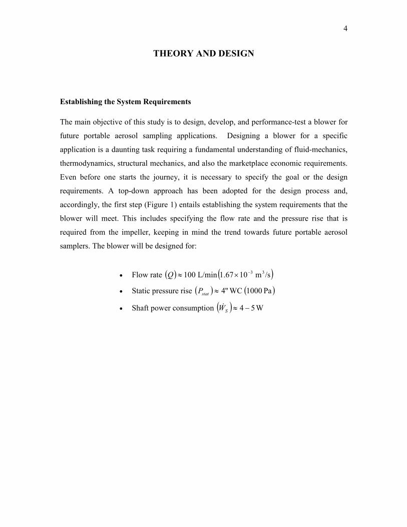
samplers. The blower will be designed for:
• Flow rate ( ) ≈Q 100 L/min ( )/sm 1067.1 33−×
• Static pressure rise ( ) ≈statP WC"4 ( )Pa 1000
• Shaft power consumption ( ) 54 −≈SW& W

5
Figure 1: Top-down design approach framework.

6
Blower Type Selection
Having established the design requirements, the next step is to decide upon the blower
type. This is a critical question as the performance of the overall system depends on using
the right pump-type for the right-application. The two broad classes of pumps are
(Japikse et al. 1997): turbo-machinery (rotating) class, and the positive displacement
class. At this point it is important to distinguish between the two – if the work done is
readily described by force, F, times distance, then it is a positive displacement pump
working by applying a force through a prescribed distance. By contrast, if the energy
transfer is described by the torque times the angular velocity then it is a turbomachine.
Further, within the turbo-machinery class there are the two extreme types: centrifugal and
axial. Centrifugal pumps produce a large head rise since the work input, and the
consequent head rise, is proportional to the impeller exit tangential speed squared ( )2U . If
the rotational rate is constant, the head rise is also proportional to the square of exit
radius ( )2
2R . The axial pump, lacking this attribute, achieves less head rise, but can have
large inlet area and hence can achieve very high flow rates (Figure 2). Before a decision
can be made as to which blower type would be most applicable to meet the design
requirements, one need to have insight into the selection methodology. This is outlined in
the next four sections.
(a) (b) (c)
Figure 2: Cross-sections of different pumps: (a) Radial flow (b) Mixed flow (c) Axial
flow (Hydraulics Institute).

7
Scaling and Similitude
Scaling and non-dimensional study of the equations governing the performance of a
system is a powerful tool. Scaling is important because if one has the set of
characteristic curves for a given pump, then that machine can be used as a ‘model’ to
satisfy similar conditions of service at different speed and a different size1. Blower
selection, design, and performance are influenced primarily by fluid dynamics,
represented by the velocity components at the various spatial points. In the literature
different notations are used to define the velocity components. To avoid any confusion,
the notation used to define the velocity components is explained below. Throughout the
thesis the NASA system of capital letters WVU and ,, is employed where:
=U tangential speed rΩ of the point on the impeller at radius r , m/s
=V absolute velocity of the fluid, m/s
=W velocity of fluid relative to rotating impeller, m/s
Scaling a given geometry to a new size means multiplying every linear dimension of the
model by the scale factor, including all clearances and surface roughness elements. The
performance of the model is then scaled to correspond to the scaled-up model by
requiring similar velocity diagrams and assuming that the influences of fluid viscosity
and vaporization (for pumps handling liquids) are negligible. Equations 1, 3, and 6
illustrate this. The blade velocity U (Equation 4) varies directly with rotational speed
N or angular speed Ω – and directly with size, as expressed by the radius r. For the fluid
velocity (or W) V to be in proportion toU , the flow rate Q must therefore vary as 3rΩ
(Karassik et al. 2000); hence, the “specific flow” sQ must be constant (Equation 2).
Further, as the total head ( )totHΔ is the product of two velocities, it must vary as 22rΩ ;
1 A cautionary note to be kept in mind – Strictly speaking the term pump is reserved for devices that use
liquid e.g. water pumps. In cases where one deals with air, using the term blower would be more
appropriate. Unfortunately, not much information is available for designing low flow rate, and low pressure
rise blowers. For the present application, since the air-flow is incompressible, the best approach is to rely
on the knowledge accrued by the pump industry. Since most of the material has been borrowed from pump
literature, the terms pump, impeller, blower have been used interchangeably throughout the text

8
hence, the head coefficient ψ must be constant (Equation 5). Finally, as power is the
product of pressure-rise and flow rate, shaft power SW& must vary as 53rΩρ ; hence, the
power coefficient must be constant (Equation 7) (Karassik et al. 2000).
3
2
3
2
22
2
R
RorNDQ
NDRV
DAAVQ
Ω⇒
Ω=
α
αα
αα [1]
and sQR
Q==
ΩConstant
3
2
[2]
)(
22DNH
UVHg
tot
HYtot
α
η θ
Δ⇒
Δ=Δ [3]
rU Ω= [4]
( )Constant
2
2
=Ω
Δ=
R
Hg totψ [5]
53DNW
HQgW
S
overall
totS
ρα
ηρ
&
&
⇒
Δ=
[6]
Constantˆ
5
2
3=
Ω=
R
WW S
Sρ
&& [7]
Uniform scaling in pump geometry or shape produces a new set of curves – shaped
differently but similar to each other. Similitude enables a designer to work from a single
dimensionless set of performance curves for a given pump model. This is a practical, but
a special, case of the more general statement. In general the performance of a pump, as
represented by efficiency, total head, and shaft power, is expressed in terms of the
complete physical equation as follows (Karassik et al. 2000):
( )ipStotoverall lSgphNPSHRQsfctWH ,,,2,,,,,,.',, 2 −Ω=Δ υρη & [8]

9
where il is the infinite set of lengths that defines the pump stage geometry. A common
group of these lengths is illustrated in Figure 3.
Figure 3: Defining the geometry of a pump stage (Karassik et al. 2000, reprinted with
permission of McGraw-Hill).

10
Non-dimensionally, Equation 8 can be expressed as:
( )ipsSoverall GQsfctW ,,,2,Re,,.'ˆ,, 2 ΣΓΦ−= τψη [9]
where the dimensionless quantities containing flow rate, viscosity and NPSH are
respectively defined as follows:
Factor Cavitation 2
Number Reynold Machine Re
Flow Specific
2
2
22
2
2
2
2
R
gNPSH
R
R
QQs
Ω=
Ω=
Ω=
τ
υ [10]
• 2
RlG ii = defines the dimensionless geometry or shape
• Φ−2 = the dimensionless quantities arising from the set of fluid, thermal,
vaporization, and hear transfer properties ph−2 that influence the flow of two-
phase vapor and liquid.
• Σ = the dimensionless quantities arising from the set of properties associated
with entrained solids and emulsifying fluids that affect the performance of slurry
pumps and emulsion pumps.
Equation 9 represents the most general treatment for describing the performance of an
impeller. For the present design, since one is dealing with air, the factors corresponding
to two-phase flow ( )Φ−2 , entrained and emulsifying fluids Σ , and the cavitation
factor 2τ , are eliminated. Hence:
( )isSoverall GQsfctW Re,,.'ˆ
,, =&ψη [11]
Equation 11 states that if we know all the quantities on the right hand side, then the
efficiency, head, and power characteristics are fixed. Therefore, pump performance is a
function of pump geometry, flow rate, and the machine Reynolds number.

11
Specific Speed and Optimum Geometry
Ideally, the hydraulic geometry or shape of a pump stage can be chosen for given values
of the other independent variables in Equation 11 to optimize the resulting performance.
One restricts the operational range of the pump by imposing certain constraints on the
head and power. Two such conditions that are common are
a) no positive slope allowed anywhere along the QvsH tot Δ−−Δ . curve (this
ensures stable pump performance (Tuzson 2000)).
b) the peak power consumption must occur at the best efficiency point (BEP) (often
called the “non-overloading” condition)
This means that by specifying the flow-coefficient, the operational machine Reynolds
number, and the head and power coefficients, Equation 11 can be used to generate the set
of geometric lengths that maximizes the best efficiency BEPη . This is the direct design
approach.
This direct design approach is rarely practical to implement. One simplifies Equation 11
using certain assumptions, and this will lead to a single dimensionless number, specific
speed ( sΩ ), a well-known figure of merit, that characterizes the geometry of fluid
machinery. One assumes that a typical pumping situation involves:
• Negligible influence of viscosity as long as the flow is principally in the turbulent
regime (a frequent situation for most, but not all, pumps (Japikse et al. 1997,
Karassik et al. 2000). Pump performance will change with Reynolds number to a
small power of approximately 0.15 to 0.2 (Japikse et al. 1997). This effect is
usually set aside for later correction or ignored completely.
• the geometry can be represented by a single characteristic size 2R (impeller blade
tip radius).

12
In this situation, Equation 11 is left with one significant independent variable; namely,
the specific flow sQ . One does not know the size of the pump stage a priori; so, 2R is
eliminated by replacing sQ in Equation 11 with a new quantity that is the result of
dividing the square root of sQ by the 4/3 -power of the head coefficient ψ . Thus, from
the definitions just given, we arrive at the specific speed sΩ as the independent variable
in terms of which the geometry is optimized (Sabersky et al. 1966).
( ) 43
43
ψ
s
tot
s
Q
Hg
Q=
Δ
Ω=Ω [12]
For convenience, specific speed is usually expressed in terms of the conventional
quantities, for example, the form found in the United States and its relationship to sΩ is
as follows:
[ ] ( )
016.2733016.2733
(ft) )(GPM (rpm) ,
43
US USstot
s
NHQN=
Δ=Ω [13]
Rotor Shape as a Function of Specific Speed
Optimization of pump hydraulic geometry in terms of best efficiency point (BEP)
specific speed has taken place empirically and analytically throughout the history of
pump development. An approximate illustration of the results of this process for pump
rotors or impellers is shown in Figure 4. Not only does the geometry emerge from the
optimization process but also the head, flow, and power coefficients for each shape as
well. Figure 4 also shows the approximate values for the optimum BEP head
coefficientψ . As can be seen, the specific speed of the application suggests the most
efficient configuration: centrifugal, mixed flow, or axial turbomachines, depending on
increasing specific speed (Tuzson 2000). Since specific speed is based on fundamental

13
physical principles (Tuzson 2000), and not an arbitrary classification, it can also be used
to characterize the operational range of positive displacement pumps (Balje 1962,
Cartwright 1977). Figure 5 further refines the choice of impeller profiles for a given
specific speed.
Figure 4: Optimum geometry as a function of BEP specific speed (Karassik et al. 2000,
reprinted with permission of McGraw-Hill).
Figure 5: Specific speed values for different pump designs (Hydraulics Institute).
14
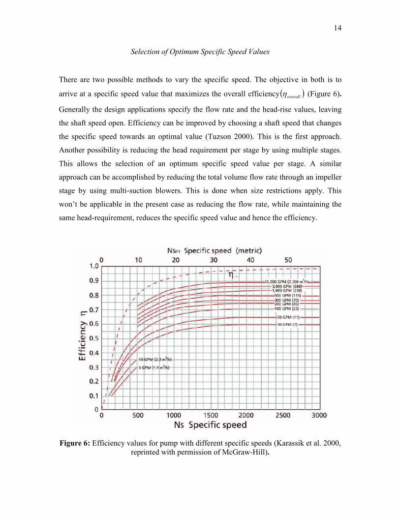
Selection of Optimum Specific Speed Values
There are two possible methods to vary the specific speed. The objective in both is to
arrive at a specific speed value that maximizes the overall efficiency ( )overallη (Figure 6).
Generally the design applications specify the flow rate and the head-rise values, leaving
the shaft speed open. Efficiency can be improved by choosing a shaft speed that changes
the specific speed towards an optimal value (Tuzson 2000). This is the first approach.
Another possibility is reducing the head requirement per stage by using multiple stages.
This allows the selection of an optimum specific speed value per stage. A similar
approach can be accomplished by reducing the total volume flow rate through an impeller
stage by using multi-suction blowers. This is done when size restrictions apply. This
won’t be applicable in the present case as reducing the flow rate, while maintaining the
same head-requirement, reduces the specific speed value and hence the efficiency.
Figure 6: Efficiency values for pump with different specific speeds (Karassik et al. 2000,
reprinted with permission of McGraw-Hill).

15
Even at this point, Method One, changing the rpm seems more feasible assuming that the
pressure rise and the flow rate can be achieved. Designing the application for portable use
also favors single stage. Nonetheless, both approaches are discussed in the section on
sample calculation; but first one needs to develop the equations for estimating the head
change.
Estimating Head Rise ( )totHΔ across an Impeller
To estimate the total head change across an impeller, the energy transfer equations across
a general rotating impeller need to be developed. Hydraulics or fluid dynamics has the
primary influence on the geometry of a rotordynamic pump stage. It is basic to the energy
transfer or pumping process. Action of the mechanical input shaft power to affect an
increase in the energy of fluid is governed by the First Law of Thermodynamics.
Realization of that energy in terms of pump pressure rise of head involves losses and
consequently the Second Law of Thermodynamics.
First Law of Thermodynamics
Fluid flow, whether liquid or gas, through a centrifugal pump is essentially adiabatic;
heat transfer being negligible in comparison to the other forms of energy transfer process.
Further, while the delivery of energy to fluid by rotating blades is inherently unsteady
(varying pressure from blade to blade as viewed in an absolute reference frame), the flow
across the boundaries of a control volume surrounding the pump is essentially steady, and
the First Law of Thermodynamics for the pump can be expressed in the form of the
adiabatic steady-flow energy equation (Equation 14) as follows:
++−
++=
in
e
out
eS gZV
hgZV
hmW22
22
&& [14]

16
where ρstatP
uh +=
Here, shaft power SW& is transformed into fluid power, which is the mass flow
rate ( )m& times the change in the total enthalpy (which includes static enthalpy, velocity
energy per unit mass, and potential energy due to elevation in a gravitational field that
produces acceleration at rate g ) from inlet to outlet of the control volume (Figure 7).
Figure 7: Energy balance across a control volume for a rotating impeller.

17
For incompressible fluids, Equation 14 can be rearranged in terms of head, viz:
uHgm
Wtot
S Δ+Δ=&
&
[15]
where estat
tot Zg
V
g
PH ++=
2
2
ρ [16]
The change in totH , totHΔ , is called the “head” of the pump; and, because H (Equation
15) includes the velocity head gV 22 and the elevation head eZ at the point of interest,
totHΔ is often called the “total dynamic head” (Karassik 2000)
Sample Calculations for Impeller Specific Speed
For calculation of specific speed, )(rpmN , the volume flow rate ( ))(USgpmQ and the total
head rise ( ))( ftH totΔ values are needed. The approach of selecting an impeller type can
be summarized as follows:
• Choose a rpm value
• Estimate the head change
• Based on the specific speed value decide an impeller type, refer Figures 4 and 5
• Make sure that the specific speed corresponds to the point of maximum efficiency
(Figure 6), if not, change the specific speed or use multiple stages
• Calculate the impeller size using the optimum BEP head coefficient ψ given in
Figure 4.
• Iterate if needed

18
Single Stage Impeller Calculations
Sample calculation is given below. At this stage, the calculation of the velocity head is
ignored, as the impeller size is not known. Instead one assumes that the effect of the exit
velocity has been included in the pressure rise value that is used in the calculations. The
following values are chosen:
• rad/s 1570~rpm 15000 Ω→=N
• USGPM 4.26~L/min 100=Q
• Pa 1000=Δ totalP
• ρ = 1.225 kg/m3 (Bleier 1997)
• 0=Δ eZ (we are dealing with air, so elevation head is negligible compared with
pressure and velocity heads)
Therefore,
( )( ) ft 273.3 m 3.830m/s 8.9.kg/m 225.1
Pa 100023
==+=Δ≈Δ stattot HH [17]
and,
[ ]( )( )
( ) 75.0
5.0
US
43
5.0
US
43
US
)(,ft
GPM.rpm1147
ft 3.273
GPM 4.26.rpm 15000
(ft)
)(GPM (rpm) ==
Δ=
tot
USsH
QNN
…[18]
This value of specific speed corresponds to a centrifugal type impeller (Figure 4). The
expected efficiency is about 0.58 (Figure 6). The efficiency value is not the maximum
possible at this flow rate, which suggests that a higher rpm value could increase the
efficiency. These points are further discussed in the next section, but before that, impeller
calculations for a two stage impeller are given.

19
Two Stage Impeller Calculations
For the two impeller model, all the variable values are kept the same. Only difference is
in the head-rise value per stage. Assume that when two stages are employed, the head
produced per-stage will be approximately half the total value (Karassik 2000). The
following values are chosen for the two stage impeller calculations:
• rad/s 1570~rpm 15000 Ω→=N
• USGPM 4.26~L/min 100=Q
• Pa 1000=Δ totalP
• ρ = 1.225 kg/m3 (Bleier 1997)
• 0=Δ eZ
Therefore,
( )( ) ft 137 m 2
3.830
m/s 8.9.kg/m 225.1
Pa 2100023, ==+=Δ −stagepertotH [19]
and,
[ ]( )( )
( ) 75.0
5.0
US
43
5.0
US
43
US
)(,ft
GPM.rpm1930
ft 371
GPM 4.26.rpm 15000
(ft)
)(GPM (rpm) ==
Δ=
tot
USsH
QNN
… [20]
This corresponds to a mixed-flow impeller (Figure 4). Further, Figure 6 shows an
expected efficiency value of 0.60. This is not an appreciable difference when compared
with the single stage centrifugal blower. Besides, using a higher rpm value with the single
stage centrifugal blower can get us to this efficiency value.
Because the same performance level can be achieved with a single stage centrifugal
blower, there is no reason in to use a two stage mixed flow impeller. Further, the two
stage impellers will lead to portability challenges, and also rotordynamic balance
problems. Also, a multi-stage axial fan will have inter-stage transfer losses that might
20
reduce the performance. Therefore, a single stage centrifugal blower was selected as the
design configuration.
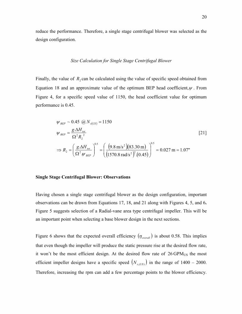
Size Calculation for Single Stage Centrifugal Blower
Finally, the value of 2R can be calculated using the value of specific speed obtained from
Equation 18 and an approximate value of the optimum BEP head coefficient,ψ . From
Figure 4, for a specific speed value of 1150, the head coefficient value for optimum
performance is 0.45.
( )
( )( )( ) ( )
"07.1m 027.045.0.rad/s 8.1570
m 30.83.m/s 8.9
.
.
.
1150@ 45.0~
5.0
22
25.0
22
2
2
2
==
=
Ω
Δ=⇒
Ω
Δ=
=
BEP
tot
totBEP
USsBEP
HgR
R
Hg
N
ψ
ψ
ψ
[21]
Single Stage Centrifugal Blower: Observations
Having chosen a single stage centrifugal blower as the design configuration, important
observations can be drawn from Equations 17, 18, and 21 along with Figures 4, 5, and 6.
Figure 5 suggests selection of a Radial-vane area type centrifugal impeller. This will be
an important point when selecting a base blower design in the next sections.
Figure 6 shows that the expected overall efficiency ( )overallη is about 0.58. This implies
that even though the impeller will produce the static pressure rise at the desired flow rate,
it won’t be the most efficient design. At the desired flow rate of 26 GPMUS the most
efficient impeller designs have a specific speed ( ))(, USsN in the range of 1400 – 2000.
Therefore, increasing the rpm can add a few percentage points to the blower efficiency.

21
By operating at a higher rpm the specific speed is increased and the impeller efficiency
approaches a limiting value of 0.60. Operating at a higher rpm value implies a smaller
impeller size. Therefore, the trend points towards smaller size and higher rpm. Increasing
the rpm value beyond a certain limit is not effective as the maximum attainable efficiency
curve flattens out as the specific speed value is increased.
A combination of 000,15 rpm and an impeller size 2D = 2.14-inches will fulfill the
requirements, but it won’t be the best possible combination. Another important point to
be considered is the value of the velocity head at the exit. At the exit, velocity is
41.42~ 22 =ΩRV m/s (or less if centrifugal blower with backward curved (BC) blades is
chosen (Karassik 2000)); implying that the magnitude of the velocity head ( )gV 22
is 8.91 m. This is of the same order as the overall pressure rise head; meaning that the
total head produced by the impeller will be more than 83.30 m. Hence, the actual specific
speed value at 15,000 rpm will be lower than what was calculated in Equation 18. This
also suggests using a higher rpm value than 15,000. But as a first approximation, the
approach is adequate to help determine the impeller type and the range of the impeller
size. Calculations for specific speed values and impeller sizes for different rpm values are
given below in Table 1.
From the table it can be observed that all the specific-speed values fall within the range
that corresponds to centrifugal impellers. Hence the impeller type is fixed: Centrifugal
type blower and it is a single stage configuration. Combinations of rpm and impeller size
that can be expected to show the best efficiency are shown as boldface in Table 1. Figure
6 further shows that beyond a specific speed value of ~2000, the efficiency does not
change This implies that increasing the rpm beyond a certain value (say ~30,000; after
accounting for the velocity head) won’t lead to any gain in efficiency. This point is
further elaborated below.

22
Table 1: Specific speed values and blower sizes at different rpms.
RPM )(, USsN Impeller
Type BEPψ
(Figure 4)
R2 (m) R2
(inch)
D2
(inch)
5000 382 Centrifugal 0.6 0.070 2.8 5.6
10000 764 Centrifugal 0.5 0.040 1.5 3.0
15000 1147 Centrifugal 0.45 0.030 1.1 2.2
20000 1529 Centrifugal 0.45 0.020 0.8 1.6
25000 1911 Centrifugal 0.45 0.016 0.6 1.2
30000 2294 Centrifugal 0.4 0.014 0.6 1.2
35000 2676 Centrifugal 0.4 0.012 0.5 1.0
40000 3058 Centrifugal 0.4 0.011 0.4 0.8
Before any conclusions are drawn, there are two more important ratios to be considered.
One of them is the ratio of pressure to velocity-head, shown in Table 2. Second is the
ratio of flow rate and rpm ( )rpmgpm , shown in Figure 8.
Although the ideal value of pressure to velocity-head ratio is not mentioned in the
literature, it must be kept low. This is because, for a given pressure head, if the velocity-
head is increased, then the energy given by the impeller is being used to accelerate the
air, which is discarded. Hence the high velocity head is not utilized. Even if one plans to
recover the velocity head as static pressure – using a diffuser, the process will have low
efficiency because of flow separation caused by adverse pressure gradients.
Further, from Figure 8, for a fixed flow rate, as the rpm is increased, the maximum
attainable efficiency value is reduced. At an rpm of 20,000 the ( )rpmgpm ratio is
0.0013, which is just about the lower limit shown in Figure 8. Therefore, one would want
to operate at the lowest possible rpm that ensures a high enough specific speed to get the
maximum efficiency.

23
Table 2: Ratio of pressure head and theoretical velocity head for different rpm and
impeller diameter combinations.
RPM R2 (m)
)(~ 22 RV Ω
(m/s) g
VH vel
2~
2
2Δ statHΔ vel
stat
H
H
Δ
Δ
5000 0.070 36.8 69.4 83.3 1.2
10000 0.039 40.4 83.3 83.3 1.0
15000 0.027 42.5 92.5 83.3 0.9
20000 0.020 42.6 92.5 83.3 0.9
25000 0.016 42.6 92.5 83.3 0.9
30000 0.014 45.2 104.1 83.3 0.8
35000 0.012 45.2 104.1 83.3 0.8
40000 0.011 45.2 104.1 83.3 0.8
Figure 8: Efficiency ( )overallη of centrifugal pumps versus specific speed, size, and shape
(Anderson 1980).

24
Summary of Findings
A single stage configuration is the best suited to meet the design requirements. The
blower type is centrifugal, the specific type of centrifugal blower has to be determined
(Bleire 1997). An rpm range of 000,30000,20 − with an impeller size of 1 – 2”, will
result in the best efficiency. This is as far as one can go theoretically. These points will
have to be verified through CFD simulations and experimental data.
Major conclusions from this section are summarized below:
• Blower configuration: single stage
• Impeller type: Centrifugal blower
• Specific speed value to ensure highest efficiency approximately 1500 – 2000 (US
units)
• rpm value in the range of 20,000 – 40,000 (lower end preferred)
• Impeller size expected ( )2D about "2 (.05m) in diameter
• Exit velocity head of considerable magnitude, especially at higher rpm values
• Velocity head can be converted to static pressure using a diffuser
Further, since the blower type has been determined to be centrifugal, referring to the
pressure value of 1000 Pa as ‘low’ is seems appropriate. Next step (Figure 1) is to
determine a base blower design that can be simulated numerically using computational
fluid dynamics software (FLUENT 6.1.22, FLUENT, Inc. Lebanon, NH). The subsequent
sections cover this.

25
BLOWER BASE-DESIGN SELECTION
According to a European Commission report (2001), pumps are the single largest user of
electricity in industries of the European Union. This observation would probably hold for
other industrialized countries as well. It is understandable that considerable research has
been performed to improve the design and performance of pumps. Indeed, during the last
5 years, the world has generated an average of 400 new patents per year in relation to the
design of blowers alone (Mann 2004). It is natural to assume that the blower design has
achieved considerable maturity, and the available designs can be modified to meet future
design requirements.
Ideally, the selection of a blower design is a simple task. Once a blower configuration
and type is finalized, based on the system requirements (described earlier in the section
on blower type selection), one consults the promotional literature of a blower
manufacturer and chooses from the range of blower designs and sizes. Referring to a
catalogue for the present case was not possible as it appears that most of the available
literature pertains to large flow rate, high pressure, and high power consuming water-
pumps.
In the absence of relevant information and off the shelf designs for low-flow rate, and
low pressure rise blowers, one is left with two possible design approaches. The first is to
start from ground zero and use the basic design principles, rules of thumb, and
computational fluid dynamics (CFD) develop the entire geometry − the blade shape, the
inlet and exit angles, leading edge shape, etc., for the centrifugal blower. This is the
direct design approach mentioned earlier. It is an arduous task. In the literature this
approach is used, albeit very rarely, when dealing with specific diverse pump
performance problems and extremely different design conditions. Examples include
pumps for fuel handling, heart pumps, pharmaceuticals, and such specialty cases. It is

26
always easier, and practical, to modify an existing high efficiency design than to recreate
a new blower design. This is covered next.
The other possible alternative is to build on a blower design already available. Here one
starts off with a general survey of the available impeller technology, to select a base
blower design. To confirm that the blower is well designed, experiments are carried out
and design features compared with the recommendations given in the literature. Once a
design is fixed, the internal flow-field is studied using CFD. The reasoning being that the
development of new and improved centrifugal fans requires the flow-field within the
impeller passages to be better conditioned than has been historically possible using
empirical overall fan performance test techniques. The objective is to identify, and then
eliminate separated and poorly conditioned flow regions. This is essential if the
aerodynamic efficiency and pressure development of the blower is to be improved.
Besides optimizing the geometry using CFD, fan scaling is used to provide the
appropriate size to meet the design goals. The guidelines developed in the preceding
sections are used for this.
Non-traditional Scaling
Conventionally, fan scaling has been oriented towards maintaining the dimensional
similarity and it has focused, for the most part, on scaling up rather than scaling down.
To maintain dimensional similarity, all dimensions (for example, diameter, width etc.)
are scaled by the same ratio. In practice errors do occur, as it is not possible to scale such
things as material thickness, or even material roughness. Another area where departures
from dimensional similarity occur is the inlet cone clearance on centrifugal fans. Usually,
however, in the relative sense these clearances are reduced with increasing size which,
more often than not, aids fan performance. Also the roughness of the impeller and case
material, over which the air passes, will remain constant as it is scaled up. This leads to
what is known as the scale effect where, in general, a larger fan will be more efficient
than a smaller one. This happens because the ratio of the static boundary layer to actual

27
flow area decreases with increasing size (Halstead 2004). A manufacturer prefers scaling
up because of the scale effect and as it allows them to perform model testing on smaller
blowers. Increases of 2 − 3% are achievable with scaling factors of 2.5 to 3; indeed,
scaling down is frowned upon in some cases (Halstead 2004).
To overcome these limitations, incorporating CFD into the design process is useful.
Using CFD, non-traditional scaling can be used and the ill effects of scaling down can be
characterized. Non-traditional scaling refers to the ability to scale different blower
dimensions independently of each other, and to visualize their effects. This is a powerful
tool, made possible by CFD. It allows better customization of the blower to meet the
design requirements. Further, performance reduction, as the blower is scaled down, can
be observed and this aids in the design process.
Design Approach
Preceding discussion points towards the modification and scaling of an existing efficient
design as the logical design approach. The approach is more representative of reverse
engineering. Customized development of a blower from ground zero to meet the design
requirements may produce the best design, but the experience required and the
investment needed, in terms of time and money, make it a non-viable option, and even
then performance improvement is not guaranteed. Going about the blower design process
from ground zero can be a future recommendation, if acceptable performance levels are
not achieved. Even though scaling-down a blower might compromise a few efficiency
points, it is the best suited as it recognizes the fact that the pump industry has matured in
its design.

28
Probable Base Blower Designs
The Aerosol Technology Laboratory (ATL) of the Texas A&M University System had
been experimenting with certain commercially available blowers for another research
project. These blowers are being used on aerosol sampling systems designed for high
flow rates ( )L/min 0100~ , and high pressure rise ( )Pa 7500or WC"30~ . The power
consumption was about 600 W (Moncla 2004). Even though these values are an order of
magnitude higher then the design requirements the blowers can be used as a probable
initial design and their performance measured. The impellers used in these blowers are
centrifugal turbo blowers (Bleier 1997) with nine ( )9Z backward curved (BC) blades.
Another appropriate place to look for air-handling centrifugal blowers is the hand-held
vacuum systems (HVS) available in the market. It can be reasoned, that the fans used in
these hand-held systems should be a product of good engineering design. Firstly, these
portable vacuum systems are battery operated, therefore the fans used in them need to be
as efficient as possible to maximize performance and endurance. An improvised home-
made experiment, with one of these blowers, showed that the system generate a suction
pressure of about "108 − WC ( )Pa 2000~ . Even though the overall efficiency of these
systems might be low as they run on small, cheap, off-the-shelf direct current (DC)
motors, the blower design has to be good for it to generate "108 − WC ( )Pa 2000~ of
pressure and a reasonable flow rate. These also have nine blades. The two blowers are
shown below (Figures 9 and 10). Design differences between the two blowers are
apparent.

29
Figure 9: Turbo blowers with backward curved blades (shroud removed).
(a) (b)
Figure 10: Hand-held vacuum system centrifugal blower (a) Top-view (b) Side-view
showing the blades.

30
Selection of the Hand-held Vacuum System (HVS) Blower: Justification
The two blowers mentioned in the last section were:
• Turbo blowers (Bleier1997), with slightly backward-curved (BC) blades, being
already tested by the lab (Figure 9)
• Centrifugal blowers, with backward-curved (BC) blades, (Bleier1997) adopted
from hand-held vacuum devices (Figure 10)
Comparison between the two designs suggests that not much engineering was
incorporated into the design of turbo-blowers. Their blades are narrow, circular arcs of
uniform height, and are riveted to the back plate and shroud. In contrast, the HVS blower
with BC blades has blades that vary in height from the leading edge to the impeller tip.
Another important factor favoring HVS blowers over turbo-blowers was the shape of the
leading edge. The design of the impeller leading edge is particularly important (Japikse
1997). Figure 11 shows a series of different inlet configurations. Turbo-blower, shown on
the left (a), is a simple two-dimensional blade following a region of moderately sharp
shroud line curvature. This is a poor design feature and can lead to separation and
backflow out of the impeller eye (Figure 12). The centrifugal blower with BC blade has a
moderately three-dimensional shaped impeller (c in Figure 11) inlet. This allows for
better incidence control (Japikse 1997).
Figure 11: Variety of common pump impeller meridional views from low to high
specific speeds (a – f) and with inducer (g).

31
Further, according to their blade shapes, centrifugal fans can be subdivided into six
categories (Bleire 1997): Airfoil (AF), backward-curved (BC), backward-inclined (BI),
radial-tip (RT), forward-curved (FC), and radial blade (RB). Figure 13 shows these six
commonly used blade shapes. Each of them has its advantages and disadvantages.
Accordingly, each is well suited for certain applications. Figure 13 also shows the
approximate maximum efficiencies that usually can be attained with these blade shapes
(these efficiency values are for large flow rate fans used in the industry, but the trend
should remain the same for smaller sized blowers). Just on the basis of the maximum
efficiency attainable, the hand-held vacuum blowers are a better choice.
Figure 12: Impeller with strong inlet curvature (a) Separation with reattachment (b)
Complete separation without reattachment.

32
Figure 13: Common centrifugal fan blade shapes.
It can be argued, based on the efficiency values (Figure 13), that AF centrifugal blowers
will be a better choice. Still, it was decided to go ahead with BC blades as these are easier
to manufacture. Besides, in centrifugal fans, the improvement due to AF blades is not as
pronounced (Bleier 1997) as the airfoil lift contributes only a small portion to the
pressure produced, and most of it is generated by the action of the centrifugal force.
In view of these arguments, the HVS blower with backward curved blades and inclined
leading edge (referred as ‘blower’ through the remaining text) was chosen as the design
base. The performance level of the blower will have to be determined, both numerically
and experimentally, to verify that the design is acceptable. This is done in the following
sections. Other dimensions, describing the blower geometry, are presented in the section
on CFD (Figure 14).

33
COMPUTATIONAL FLUID DYNAMICS (CFD)
Background
The objective here is to design, develop and test a centrifugal blower to meet the specific
flow rate and pressure rise requirements, and have acceptable efficiency levels.
According to Turton (1984) a successful impeller design should, “…produce a specific
pressure rise and flow rate within acceptable limits, at an acceptable rotational speed, and
require minimum power from its drive; also, it must exhibit stable characteristics over the
operating range required. The impeller must be as small as possible, the power absorbed
must be non-overloading over the flow range and the noise and vibration must be within
specified limits. The design must always be economical, give good quality assurance, and
be easily maintained…”
Designing a blower that meets all the above mentioned parameters is a daunting task and
a challenging research area. To design an impeller, it is necessary to predict its
performance curves. Performance prediction design process has classically evolved from
a fully empirical process in the 1950’s, through to a one dimensional analysis in the
1960’s. It continued with the axis-symmetric through flow calculations in the 1970’s,
with full three dimensional calculation of the blade to blade flow field becoming routine
during the 1980’s (Tallgren 2004). Early 1990’s saw the development of Quasi Three-
dimensional Analysis (Q3D) technique as a blade design tool (Katsanis 1991).
Flow patterns in a centrifugal pump are three-dimensional, unsteady, and characterized
by re-circulation, cavitation (for water pumps), and pressure pulsations. The early
methods cannot handle the complexity of such flow-phenomenon. Hence, the later part of
1990 saw increase in computational capability enable the use of three-dimensional
computational techniques during the design process itself (Tallgren 2004), instead of just
the post design analysis of blade performance.

34
Ever increasing computational power and robust turbulence models enabled CFD to
become a powerful tool. Solving three dimensional Reynolds-averaged-Navier-Stokes
equations has become routine. CFD has been used to predict recirculation, and the results
compare favorably with experimental data (Graf 1993). Gülish et al. (1997) predicted the
entire performance curve of head within about two percent, and the power curve with
slightly less accuracy. Lakshminarayana (1990) assesses the use of CFD techniques in the
analysis and design of turbo-machinery. Further, CFD is being used in the design of
unconventional pump applications, like blood pumping devices (Koh 1999). All this
highlights the fact that CFD allows a systematic, robust, and economically viable
approach to pump design.
CFD Approach
A common factor applicable to all CFD studies of turbo-machinery is that the CFD does
not eliminate the need for experimental validation; it does however compliment it. This is
achieved by using measurements, which are relatively quick and easy to make, to verify
that a CFD model is producing results that are predicting the overall performance
correctly. The CFD model can then be assumed to model the flow adequately and as such
used to provide information on the flow-field. This is exactly the approach taken here.
Once we have confidence that CFD is predicting the measured performance of a blower
reasonably accurately, a study of the CFD results facilitates insights into aspects of the
flow field that are limiting fan performance. This in turn offers the possibility of making
changes to the CFD model in an attempt to improve the predicted performance (non-
traditional scaling). Once predicted performance has been improved, possibly after many
different design iterations, the optimized geometry is fabricated, and overall fan
performance again verified empirically.
The above two paragraphs describe the essence of the remaining thesis. The blower
model will be built in a Computer Aided Design (CAD) package, Inventor 8 (Autodesk

35
Inc., San Rafael, CA). The performance of the blower will be predicted using a
commercial CFD package – FLUNET 6.1.22 (FLUENT Inc, Lebanon, NH). Predicted
blower performance will be validated against experimental results; for this an
experimental test rig will be designed (explained in the subsequent sections). Once CFD
predictions are in general agreement with the experimental data, changes to the blower
model will be made; these include changing the impeller size, the blade height, etc. to
achieve improved predicted performance at the design point. Then the optimized fan
geometry can be fabricated, and overall fan performance again verified experimentally.
An additional advantage of CFD, mentioned earlier, is the flow visualization that is
possible. This helps understand how different flow features such as separated flow
regions or secondary flow vortices, are developing through the fan. To gather sufficient
data to do these using empirical techniques is simply impractical in practice.
FLUENT 6.1.22 - Introduction
FLUENT 6.1.22 is a state-of-the-art Computational Fluid Dynamics (CFD) program for
modeling fluid flow and heat transfer in complex geometries. FLUENT uses the finite
volume (FV) formulation to discretize the governing equations of mass conservation,
force balance, energy conservation (if needed), and species conservation (for multiphase
modeling) over complex problem domains. To support these functions FLUENT
incorporates an extensive range of turbulence models, buoyancy models, species
transport models, etc. (FLUENT User’s Guide 2004).
Any modeling approach using CFD has the following sequence:
• Physical model is either created in the geometry setup module or is imported from
other standard CAD design packages
• The physical model is meshed. This is a critical step as the mesh used should be
able to capture the flow physics
• A physical model has to be chosen depending on the type of flow being modeled,
for example, inviscid, laminar, or turbulent

36
• Various boundary and initial conditions are specified
• The discretized representation of the governing equations over the flow domain is
solved
• Post processing and analysis of the flow solution is done
In FLUENT these functions are split between GAMBIT and the FLUENT solver.
GAMBIT is used to define the geometry and create the mesh. GAMBIT offers great
flexibility in meshing the problem domain and allows for triangular, quadrilateral,
tetrahedral, or hexahedral cells. The grid can be structured or unstructured.
The FLUENT solver defines the physical model i.e. laminar, turbulent, combustion,
multiphase, etc., specifies the various boundary conditions, solves the finite volume
equations over the discretized domain, and post processes the results. An inbuilt post-
processor is a useful feature available in FLUENT.
Blower Geometry for CFD Simulations
The hand-held vacuum system (HVS) blower geometry was created in Inventor 8. Most
of the dimensions could be easily measured except for the inlet blade angle, the exit blade
angle, and dimensions of the blower leading edge. These values were approximated. The
blower geometry, with the characteristic dimensions, is shown in Figure 14.
The main characteristic dimensions of the blower are:
• Impeller eye diameter ( ) "58.1=ed ( )mm 40
• Impeller outlet diameter at blade trailing edge ( ) "7.22 =D ( )mm 6.68
• Impeller blade height at exit ( ) ( )mmb 4.7"29.02 =
• Blade angle at leading edge ( ) oo 05.23 and 07.131 =β
• Blade angle at trailing edge ( ) oo 92.31 and 92.282 =β

37
Figure 14: Base blower dimensions (mm).
38
GAMBIT Model
The geometry of the blower is rotationally symmetric. This implies that one can divide
the blower geometry into sections since that the flow physics in each section is the same,
except for the rotation about the axial direction. This reduces the computational effort as
it requires only one passage of the impeller to be simulated. The approach of simulating a
single blower passage is common in literature (Han et al. 2002). The only probable
drawback might be slightly lower exit velocities as the blade thickness is not incorporated
in the model
In the present case, the blower has 9 blades, implying that a computational domain
bounded by the blade profiles and with an included angle of o40 will be adequate to
capture the flow-field. The GAMBIT model is shown in Figure 15. The volume was
closed by extending the blade walls to the origin of the rotation axis. To do this, periodic
boundary conditions: periodic boundary – a, and periodic boundary – b (Figure 15), were
created. Periodic boundary conditions are used when the physical geometry of interest
and the expected pattern of the flow/thermal solution have a periodically repeating nature
(FLUENT User’s Guide 2004).

39
Figure 15: CFD model created in GAMBIT.
GAMBIT Meshing
An acceptable mesh is crucial in reaching a converged solution that captures all the key
parameters of the flow. On the other hand, too many nodes in the system may increase
the computational resources and time without providing additional resolution. These two
requirements go against one another. Generating the mesh is a critical step in CFD
analysis. A mesh captures the flow physics and requires considerable experience with
CFD and an ability to visualize the flow. General guidelines do exist for creating
acceptable meshes (ERCOFTAC Best Practice Guidelines 2000, GAMBIT 2.1 User’s
Guide 2004).

40
For the present case, hexahedral mesh elements were used all through the CFD model
and hence, the grid was the structured type. Cooper meshing scheme was used in which a
face is meshed first, called the source face. The source face-mesh is translated through
the volume. The mesh is shown in Figures 16 (a) and (b). The face representing the mass
inlet was meshed using tri-primitive mesh scheme with quadrilateral elements. This was
done due to the shape of the inlet faces. The impeller shroud face was meshed using
quadrilateral elements and submap meshing scheme (GAMBIT User’s Guide 2004).
Figure 16: CFD model mesh: (a) Top-view

41
Figure 16: continued: (b) Side-view
Mesh-quality was verified using the equiangle skew algorithm (GAMBIT User’s Guide
2004). Each element has a value of skewness between 0 and 1, where 0 represents an
ideal element. Values less than 0.98 are acceptable. For the present case, because of the
complex shape of the flow-domain, majority of the elements have a skewness value less
than 0.8. This information is represented in a histogram, with the skewness values on the
horizontal axis. Figure 17 shows the skewness distribution for the blower mesh. The total
number of grids cell was 14000.

42
Figure 17: Mesh quality: Skewness value for mesh cells.
FLUENT Model
Fluid flow in a rotating machine is characterized by a rotational (or machine) Reynolds
number, Re. It is defined based on the rotational speed ( )rad/s ,Ω , the impeller exit
radius ( )m ,2r , fluid density ( )3kg/m ,ρ , and the dynamic viscosity ( )kg/m.s ,µ . For the
impeller considered first in this study, the machine Reynolds number is of the order of
510 (Equation 22).
( )( )
( )( )( )( )
5
5
232
2
5
2
3
1066.1kg/m.s 107894.1
m 034.0.rad/s 2094.kg/m 225.1..Re
kg/m.s 107894.1
m 034.0
rpm 000,20rad/s 2094
FLUENTkg/m 225.1
×=×
=Ω
=
×=
=
=Ω
=
−
−
µρ
µ
ρ
R
R [22]

43
Turbulence Model
The flow field, based on the machine Reynolds number, is definitely turbulent. One has
to choose a turbulence model which encapsulates the physics of the flow and produces
the most realistic results. The simplest ``complete models'' of turbulence are two-equation
models in which the solution of two separate transport equations allows the turbulent
velocity and length scales to be independently determined. The standard εκ − (Launder
et al. 1972) model falls within this category and has been the most widely used for
engineering calculations.
The εκ − model is acceptably accurate for simple flows, but it can be quite inaccurate for
complex flows (Pope 2001). Flow within an impeller rotating at 20,000 rpm is complex.
The difficulties associated with solving swirling and rotating flows are the result of the
high degree of coupling between the momentum equations, which is introduced when the
influence of the rotational terms is large. A high level of rotation introduces a large radial
pressure gradient that drives the flow in the axial and radial directions. This, in turn,
determines the distribution of the swirl or rotation in the field. To account for these
factors, improvements have been made to the εκ − model. One such variant, used here,
is the Renormalization Group (RNG) εκ − model (Yakhot 1986). FLUENT
recommends using RNG εκ − model for highly swirling flows and provides an option to
account for the effects of swirl or rotation by modifying the turbulent viscosity
appropriately. For the transport equations the reader is referred to the FLUENT User’s
Guide (2004) and Pope (2001).
Inlet and Outlet Conditions
At the inlet boundary, a uniform axial velocity (along the Y axis) is imposed based on the
specified mass flow rate. For this, the inlet area is estimated and the inlet velocity
magnitude calculated. For the turbulence model, due to a lack of turbulence data from the

44
experiment, a turbulence intensity of %5.2 and a reference length equal to %3 of the
inlet diameter is assumed (Thakur et al. 2002). The outlet boundary is specified as mass-
flow with all other variables being extrapolated. Turbulence intensity and length scale are
calculated in a manner similar to inlet boundary.
Near-Wall Treatment
Another important consideration for turbulence modeling is the near-wall modeling.
Turbulent flows are significantly affected by the presence of walls (Tennekes et al. 1997).
Further, the εκ − models are primarily valid for turbulent core flows (i.e. the flow in the
region far from walls). Consideration therefore needs to be given as to how to make these
models suitable for wall-bounded flows. This is done with the help of wall functions
(FLUENT User’s Guide 2004). FLUENT provides two options, standard wall functions
and non-equilibrium wall functions. FLUENT recommends using the non-equilibrium
wall functions for complex flows involving separation, reattachment, and impingement
where the mean flow and turbulence are subjected to severe pressure gradients and
change rapidly. This is due to of its capability to partly account for the effects of pressure
gradients and departure from equilibrium.
A cautionary note to be kept in mind regarding the limitation of the wall functions
approach. To quote from FLUENT manual, “The standard wall functions give reasonably
accurate predictions for the majority of high-Reynolds-number wall-bounded flows. The
non-equilibrium wall functions further extend the applicability of the wall function
approach by including the effects of pressure gradient and strong non-equilibrium.
However, the wall function approach becomes less reliable when the flow conditions
depart too much from the ideal conditions underlying the wall functions”. Examples
include:
• Severe pressure gradients leading to boundary layer separations
• Strong body forces (e.g., flow near rotating disks, buoyancy-driven flows)

45
Both these conditions are relevant for the blower and restrict the applicability of wall
functions approach. FLUENT recommends using the enhanced wall treatment for such
situations. The only drawback here is that enhanced wall treatment formulation is
computationally expensive and time consuming. This difference can be understood in
terms of the non-dimensional distance +y =µ
ρ τ Pyu .., to the wall from the first grid cell.
Here ρ is the fluid density, wwu ρττ = is the friction velocity, Py is the distance from
point P to the wall, and µ is the fluid viscosity at point P. The wall functions
formulation requires a 30≈+y (ERCOFTAC Best Practice Guidelines 2000, FLUENT
User’s Guide 2004) while for enhanced wall treatment 1≈+y (FLUENT User’s Guide
2004). This translates into the number of grid cells being a magnitude higher for the
enhanced wall treatment approach. Therefore, the approach adopted here is to use the
non-equilibrium wall functions formulation initially, and then switch to enhanced wall
treatment if performance prediction is not acceptable.
In the next section, a description of the test assembly is given. The results from the
simulations and the test runs are given in a subsequent section.

46
EXPERIMENTAL TEST RIG
CFD quickens and adds flexibility to a design process. A common factor applicable to all
CFD studies of turbo-machinery is that the CFD does not eliminate the need for
experimental validation. CFDs robustness, for turbulence modeling, is still to be proved.
Further, Japikse et al. (1997) mention that for small-size pumps, the existing CFD
capability does not work well. Hence to gain sufficient confidence in the CFD model, it is
necessary to validate the simulation results with experimental data.
The approach is to make simple measurements, like pressure rise, flow rate, etc. and
compare them with the simulation results. A schematic of the test-rig, which was setup
for the present study, is shown in Figure 18. It includes a venturi (for flow rate
measurement), a valve for flow-control, the centrifugal fan to be tested, and a motor drive
mechanism. Other components are explained in the following sections. A photograph of
the set-up, showing the venturi flow-meter, the gauges for pressure measurement, and the
valve, is given below in Figure 19.
Figure 18: Blower test-rig schematic.

47
Figure 19: Blower performance measurement test-rig.
Flow Rate Measurement
A venturi flow meter (FLOW-DYNE Engineering, Inc. Fort Worth, TX) was installed as
an inlet section and used to measure the flow of air. The venturi consists of a converging
inlet section, a short straight throat section, and a diverging section. A venturi flowmeter
was selected because of the high percentage of pressure recovery possible (Figure 20).
This was needed because of the low pressure capabilities of the blower involved.
Calibration charts were provided by the company (Appendix A). Sample calculation is
also shown there. The venturi has a throat diameter ( )1D of "25.0 and an inlet section
diameter of "04.1 .

48
Figure 20: Pressure recovery for different venturi types (FLOW-DYNE Engineering).
Pressure Measurement
Pressure measurement was done using standard manometers available through Dwyer
Instruments (Dwyer Instruments, Inc. Michigan City, IN). The accuracy and the range of
the manometers were selected based on the design requirements. Pressure readings were
needed at two points: (i) Differential pressure across the venturi inlet and the throat.
Expected pressure differential was ( )Pa 3700 WC"15 , this covers a volume flow rate of
approximately L/min 200 based on the venturi calibration curves (Appendix A). (ii)
Static pressure reading is needed at the blower inlet region. The manometer here
measures the suction pressure created by the blower. The expected negative pressure
range was ( )Pa 15001000 WC"64 −− .

49
Blower Drive
FLUENT simulations need to be validated against experimental results. The approach is
to:
• Simulate the hand-held vacuum system blower
• Run tests with the blower
• If agreement is acceptable, modify the blower design to optimize performance at
the design point
• Modify the test-rig for the final design and test again
At this point, the torque requirements from the blower are not known, so an appropriate
motor cannot be selected. For testing the hand-held vacuum system blower, it was
decided to use the original motor supplied with the vacuum system. Later, once the
torque requirements are known from FLUENT an appropriate motor will be chosen.
RPM Measurement
A fiber–optic photoelectric sensor – model E3X-A11 and fiber–optic cable E32-CC200,
available from Omron Electronics (Omron Electronic Components, Schaumburg, IL) was
used to measure the blower rpm. These sensors have fast response time and adjustable
sensing distance. The small size of these sensors allowed them to be accommodated in
the limited space available. The output signal was connected to an oscilloscope which
displayed the pulse frequency. The rpm value was calculated from the displayed
frequency.

50
BASE-DESIGN SIMULATION AND EXPERIMENTAL DATA
COMPARISON
The results from the CFD run and the experimental test are given below. A simple sizing
convention, to identify the different blower types, is followed. The base-design impeller
i.e. the hand held vacuum system blower is specified as 100 units in all three ( )ZYX ,,
directions. The in-plane directions are represented by ZX and axis, while the impeller
axial direction is specified as Y . Any subsequent scaling is mentioned before the
direction name, for example the base-design blower, according to this convention, will be
named as100xz_100y. The rpm value at which a blower operates is given after the name.
Therefore, a blower named as 70xz_28y@20k has been scaled in the ZX and directions
%70 and in the Y direction by 28%, and the blower was tested at 20,000 rpm.
Blower Efficiency Definitions
At this point it is necessary to differentiate between the different efficiencies defined in
the literature. Equations 15 and 16 (reproduced below) define the energy transfer process
in an impeller. Here totHΔ represents the total dynamic head, the other terms have been
defined already.
uHgm
Wtot
S Δ+Δ=&
&
[15]
where estat
tot Zg
V
g
PH ++=
2
2
ρ [16]
As can be seen from Equation 15 not all of the mechanical input energy per unit mass
(that is, the shaft power per unit of mass flow rate) ends up as totHgΔ , i.e. as useful
blower output energy per unit mass. Instead, losses produce an internal energy increase

51
uΔ (manifested as a temperature increase). This fact is obtainable from the Second Law
of Thermodynamics and can be represented symbolically as:
1or ≤≤Δ ηm
WHg S
tot&
&
[23]
where
Qm ρ=& [24]
Blower losses are quantified by the overall efficiency ( )overallη , which must be less than
unity. The overall efficiency can be expressed as:
Efficiency Pump Overall=Δ
=S
tot
overallW
mHg
&
&η [25]
This is the value given in Figures 6 and 8. In the present case, the overall pump efficiency
value cannot be measured because there was no way, either in FLUENT or
experimentally, to determine both the numerator and denominator. Experimentally, one
can determine the shaft power SW& but cannot measure the total head change. It can be
approximated at best. For FLUENT, one can get the average total head change value, but
cannot simulate shaft power. This is because the simulation model does not predict the
disk friction losses ( )DW& . Therefore, no direct comparison can be drawn between
efficiency values given in Figure 6 and the values one gets here. Figure 6 can only act as
a benchmark. Mixing simulation values with experimental data to get overallη is not
appropriate and these values are not reported.

52
Component Efficiencies
To pinpoint the losses, it is convenient to deal with them in terms of “component
efficiencies” (Japikse et al. 1997). For the typical shrouded– or closed-impeller pump
shown in Figure 21, Equation 25 can be rewritten as follows:
( )LI
Ltot
S
Ioverall
mm
m
W
mmHg
W
W
&&
&
&
&&
&
&
+×
+Δ×=η [26]
where IW& equals the power delivered to all fluid flowing through the impeller. Also, Lm& is
the total external mass leakage past the impeller and back into the impeller inlet. The
equivalent volume leakage volume flow-rate is given as LQ (Equation 28).
Figure 21: Determining component efficiencies.

53
Noting that
( )head ideal =
=+Δ=
i
ILii
H
WmmHgW &&&&
one may rewrite Equation 26 as follows:
vHYm
Li
tot
S
Ioverall
Q
H
H
W
Wηηηη ××=
+×
Δ
Δ×=
&
&
[27]
where,
S
DS
S
Im
W
WW
W
W
&
&&
&
& −==η [28]
i
Li
i
totHY
H
HH
H
H
Δ
−Δ=
Δ
Δ= ∑η [29]
L
vQQ
Q
+=η [30]
The product of all three, i.e. mechanical efficiency ( )mη , hydraulic efficiency ( )HYη , and
volumetric efficiency ( )vη yields the overall pump efficiency as defined in Equation 26. It
reflects the following division of pump losses:
a. Disk Friction Losses ( )DW& : Disk friction is the external drag on the rotating element
due to fluid friction on the outside surfaces of the impeller shroud (Japikse et al.
1997, Gülich et al. 1997). The “mechanical efficiency” is that portion of the shaft
power that is delivered to the fluid flowing through the impeller passage. One
cannot quantify ( )DW& through the current FLUENT simulations since the entire
blower was not simulated. Only the flow internal to the impeller was considered.
The interaction with the blower housing were not included. FLUENT was used to

54
calculate the total torque required to overcome the fluid friction inside the impeller
and to produce the head and flow rate. This value of IW& was obtained by integrating
the force times the moment arm over the impeller passage surfaces.
b. Hydraulic Efficiency: Hydraulic losses, due to fluid friction, separation, etc. occur
in the main flow passages of the pump. The energy loss per unit mass
is ( )∑ Δ−Δ= HHgHg iL . The ratio of actual total output head produced totHΔ to
the theoretical head supplied to the fluid iH is the hydraulic efficiency.
c. External Leakage Losses LQ : Leakage losses totaling LQ leak past the impeller and
back into the inlet eye. This leakage flow has received its share of the full impeller
power ( )LiI QQHgW +Δ= ρ& delivered to all the fluid ( )LQQ + passing through the
impeller. The leakage power is LiL QHgW Δ= ρ& , which is lost as this fluid leaks
back to the impeller inlet. The remaining fluid input power is thus
( ) QHgWW iLI Δ=− ρ&& , the ratio of this power to the total ( )IW& being the volumetric
efficiency
As already stated, estimating overallη for the present case involves dividing the total head
change value obtained from FLUENT, with the shaft power estimated experimentally
(Equation 31). Mixing simulation values with experimental data was not deemed
appropriated, and therefore, overallη values are not reported. Instead, other efficiency
definitions are used as given in next section.
EXPS
FLUENTtot
overallW
mHg
&
&Δ=η [31]

55
FLUENT and Experimental Efficiency Definition
The FLUENT simulations can provide an estimate of IW& by integrating the force time the
moment arm over the impeller passage surfaces. Performance losses due to leakages and
hydraulic are not obtained. There is no way to quantify DW& without the use of rotary
transducers, or other setup, to measure shaft power SW& . Neither can the leakage flow rate
LQ be estimated. To overcome these limitations, modified efficiency definitions are used
through the remainder of this thesis. An important point to note is the mass flow rated
used in these definitions.
( )
( )FLUENT from Calculated
..
PowerImpeller
Rise Head Total
..
PowerImpeller
Rise Head Static
,
+Δ==
+Δ==
I
LtotalFLUHY
I
LstatFLU
W
mmHg
W
mmHg
&
&&
&
&&
η
η
[32]
( )
( )
Δ==
Δ==
S
statblower
elec
statEXP
W
mHg
W
mHg
&
&
&
&
..
Power Shaft Motor Calculated
Rise Head Static Measured
..
InputPower Electrical Measured
Rise Head Static Measured
η
η
From experiment [33]
• FLUENT Efficiency ( ) :FLUη This efficiency value is plotted in the simulation result
graphs one gets from FLUENT. It gives a measure of the effectiveness of the
blower to convert the impeller power ( )IW& into static head rise.
• Hydraulic Efficiency, FLUENT ( ):,FLUHYη Although, ( )FLUHY ,η is predicted using
FLUENT simulations it acts as a valuable reference. For a well designed blower
hydraulic efficiency values should be high
• Experimental Efficiency ( ) :EXPη It is the standard first law definition. It can be
defined asfor paidEnergy
sortEnergy . This value is plotted in the experimental data plots.

56
• Blower Efficiency ( ) :blowerη This is the best representation of actual blower
performance independent of the motor used and the velocity head generated.
Hand-held Vacuum System Blower (100xz_100y)
Blower characteristic curves, calculated using FLUENT, are given in Figure 22. The
pressure rise ( )statHΔ hence was obtained by calculating the difference of the area-
average pressure at the exit and inlet planes. As can be observed, the pressure rise is
almost constant over the flow-range simulated. Even though the blower can operate at the
design point, it won’t be efficient. Further, the design point lies on the positive slope
region of the curve. This region can produce unstable blower performance (Karassik et al.
2000, Tuzson 2000).
200
400
600
800
1000
1200
1400
0 200 400 600 800 1000
Q (flow rate), L/min
de
l P
sta
t (P
res
su
re),
Pa
FLU: [email protected]
FLU: [email protected]
FLU: [email protected]
Figure 22: FLUENT performance curves for 100xz_100y blower.
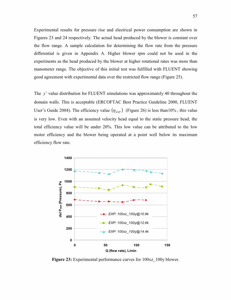
57
Experimental results for pressure rise and electrical power consumption are shown in
Figures 23 and 24 respectively. The actual head produced by the blower is constant over
the flow range. A sample calculation for determining the flow rate from the pressure
differential is given in Appendix A. Higher blower rpm could not be used in the
experiments as the head produced by the blower at higher rotational rates was more than
manometer range. The objective of this initial test was fulfilled with FLUENT showing
good agreement with experimental data over the restricted flow range (Figure 25).
The +y value distribution for FLUENT simulations was approximately 40 throughout the
domain walls. This is acceptable (ERCOFTAC Best Practice Guideline 2000, FLUENT
User’s Guide 2004). The efficiency value ( )EXPη (Figure 26) is less than %10 , this value
is very low. Even with an assumed velocity head equal to the static pressure head, the
total efficiency value will be under 20%. This low value can be attributed to the low
motor efficiency and the blower being operated at a point well below its maximum
efficiency flow rate.
0
200
400
600
800
1000
1200
1400
0 50 100 150
Q (flow rate), L/min
de
l P
sta
t (P
res
su
re),
Pa
EXP: [email protected]
EXP: [email protected]
EXP: [email protected]
Figure 23: Experimental performance curves for 100xz_100y blower.

58
0
5
10
15
20
25
30
35
0 50 100 150
Q (flow rate), L/min
Wele
c (
Ele
ctr
ica
l P
ow
er)
, W
EXP: [email protected]
EXP: [email protected]
EXP: [email protected]
Figure 24: Experimental electrical power consumption curves for 100xz_100y blower.
0
200
400
600
800
1000
1200
1400
0 50 100 150 200Q (flow rate), L/min
de
l P
sta
t (P
res
su
re),
Pa
FLU: [email protected]
FLU: [email protected]
FLU: [email protected]
EXP: [email protected]
EXP: [email protected]
EXP: [email protected]
Figure 25: FLUENT –vs. - Experimental data for 100xz_100y blower.

59
0
1
2
3
4
5
6
7
8
9
10
0 50 100 150
Q (flow rate), L/min
Ex
pe
rim
en
tal E
ffic
ien
cy
(η
EX
P)
%
EXP: [email protected]
EXP: [email protected]
EXP: [email protected]
Figure 26: Experimental efficiency ( )EXPη values for 100xz_100y blower.
Observation
CFD results compare well with the experiment measurements. The experimental
efficiency ( )EXPη of the blower is low (Figure 26); however, this can be accounted by the
motor being used to run the blower and the blower being operated at a flow rate well
below its maximum efficiency point. Recirculation and separation at low flow rates
implies that the blower has been designed for higher flow rates than100 L/min. This can
also be observed from Figure 22 which shows the maximum pressure value occurring at
600 L/min. This suggests scaling the blower down by changing the blade height – to
affect volume flow rate, and by decreasing the blower diameter – to reduce the head
produced. This is done in the subsequent sections.

60
FLUENT SIMULATIONS FOR DIFFERENT SCALING CASES
Fluent Data
Different scaling was performed in the ZX and and the Y directions. ZX and scaling
varied the impeller diameter and hence the pressure-rise across it, whereas the blade
height was reduced to change the optimum flow rate. Changing the blade height shifts the
blower characteristic curve to the left and causes the peak blower performance to occur at
a lower flow rate. Characteristic curves for several different cases are given in Figure 27.
Figure 28 presents the efficiency levels ( )FLUη predicted by FLUENT. All of these
simulations have been performed at 20000 rpm; therefore this is not specifically
mentioned in the blower name.
0
200
400
600
800
1000
1200
1400
0 100 200 300 400 500 600 700 800 900
Q (flow rate), L/min
de
l P
sta
t (P
res
su
re),
Pa
FLU: 70xz_70y
FLU: 70xz_28y
FLU: 70xz_14y
FLU: 65xz_65y
FLU: 65xz_26y
FLU: 65xz_21y
FLU: 60xz_26y
Figure 27: FLUENT performance curve for different-scaled blowers.

61
10
20
30
40
50
60
70
80
90
0 100 200 300 400 500 600 700 800 900
Q (flow rate), L/min
FL
UE
NT
Eff
icie
ncy (
ηF
LU)
%FLU: 70xz_70y
FLU: 70xz_28y
FLU: 70xz_14y
FLU: 65xz_65y
FLU: 65xz_26y
FLU: 65xz_21y
FLU: 60xz_26y
Figure 28: FLUENT efficiency values ( )FLUη for different scaled blowers.
Table 3: Sample blower simulation data.
Blower 65xz_21y@20k
Case # Q (L/min) ( )Pa statPΔ ( )N.m T ( )W IW& ( )W .. statHgm Δ& FLUη %
1 50.7 1019.0 0.00009 1.79 0.86 48.04
2 62.4 1018.8 0.00011 2.10 1.05 50.10
3 75 1003.5 0.00013 2.48 1.23 49.60
4 93.7 973.3 0.00015 2.77 1.53 54.67
5 100 954.0 0.00015 2.90 1.61 55.56
6 125 851.4 0.00017 3.20 1.76 55.19
7 140 801.6 0.00017 3.25 1.86 57.10
8 156 706.3 0.00017 3.29 1.83 55.62
9 200 357.4 0.00016 3.00 1.18 39.39
10 225 90.6 0.00014 2.60 0.34 13.04

62
A sample of the data from the FLUNET simulations is given above (Table 3). From
Figure 26, the effects of blower diameter and blade height are clearly indicated. The
efficiency value of the impeller decreases as the impeller is made smaller. However, the
overall power required to produce the 1000 Pa head at 100 L/min is less for the small,
less efficient blowers than the larger blowers which are more efficiency but require more
power to operate at the off design conditions. Trying to balance the rate of pressure
decrease and Best Efficiency Point (BEP) effect, it appears that blower 65xz_26y will
give optimum efficiency and a good performance safety margin (Table 4) under 20,000
rpm. Blower size65xz_21y could also be used, but the pressure rise versus flow rate
curve has a very steep slope providing very small margin for error and it needs a higher
rpm than 20,000 to get the pressure rise (Table 4). The characteristic curve and the
efficiency value are given below (Figure 29) for the selected blower.
Table 4: Efficiency values for different scaled blower at design flow rate.
Planar Scaling
(xz)
Axial Scaling
(y) RPM
( )Pa statPΔ FLUη %
70xz 70y 18500 1028.5 31.2
70xz 28y 18500 1025 44.96
70xz 14y 21500 1033.2 52.6
65xz 65y 19500 1031.54 48.33
65xz 26y 20000 1006.5 38.2
65xz 21y 20500 1030.5 54.5
60xz 26y 21500 1011.44 55

63
0
200
400
600
800
1000
1200
0 50 100 150 200 250 300
Q (flow rate), L/min
del
Ps
tat (P
res
su
re),
Pa s
tat
0
10
20
30
40
50
60
70
FL
UE
NT
Eff
icie
nc
y (
ηF
LU)
%
del P-FLU: 65xz_26y@20k
Design Point Pressure
ETA-FLU: 65xz_26y@20k
Figure 29: FLUENT performance curves for 65xz_26y@20k blower.
FLUNET gives the impeller power IW& as 2.9 W. Allowing for additional losses due to
the blower housing, the shaft power SW& should be less than 4 W. Experiments were
carried out with this blower, and the CFD model was validated. Before considering that,
it will be interesting to look at the non-dimensional results for the different blower sizes
simulated with FLUENT.
Non-dimensional Study for Blower Simulation Results
In the present study, non-traditional fan-scaling laws have been used to decide upon the
impeller radius ( )2R and the blade height ( )2b . The conventional fan-scaling laws are
valid (to an extent) when the scaling is uniform in all three directions. In fact, uniform

64
scaling in all three directions is an underlying assumption in the fan laws (Japikse et al.
2000). This is verified by the fact that in the traditional fan-laws the blower dimension is
represented as a single length scale ( )2R (Equations 2 and 5), and all other dimensions
scale accordingly.
3
2R
QQs
Ω= [2]
( )2
2R
Hg tot
Ω
Δ=ψ [5]
When dealing with different axial and planar scaling, the scaling law must be modified.
This was done by incorporating the blade height at the exit ( )2b into the scaling
equations. The approach was to keep the exponent of the length term same i.e. the sum of
the exponents for 2R and 2b should be equal to 3 for flow coefficient (equation 2); and
equal to 2 for the head coefficient term (equation 5). In the present case, since we are
concerned with static pressure rise value, it was decided to use only the static head term
instead of the total head term as done for conventional scaling laws (Equation 34 and 35).
3
.. 22
mod,
=+
Ω=
yx
bR
yxs [34]
and,
2
.. 22
2mod
=+
Ω
Δ=
ji
bR
Hgji
statψ [35]
Estimated values for the exponents jiyx ,,, were chosen. Simulation data for the
different blower sizes were non-dimensionalized according to Equations 34 and 35. The
process was iterated upon till an acceptable data overlap was obtained. The results are
shown below in Figure 30; all data points are at 20000 rpm except for the 100xz_100y
data points which are at 14400 rpm and provide a good cross check for scaling at
different rpm values.

65
0
50
100
150
200
250
0 5 10 15 20 25 30 35
Modified Flow Coefficient (Qs,mod)
Mo
dif
ied
He
ad
Co
eff
icie
nt
(ψm
od)
FLU: [email protected]
FLU: 70xz_70y
FLU: 70xz_28y
FLU: 70xz_14y
FLU: 65xz_65y
FLU: 65xz_26y
FLU: 65xz_21y
FLU: 60xz_26y
Trend Line
Figure 30: FLUENT non-dimensional modified head coefficient curve.
From the analysis, the modified scaling laws are given as (Equation 36)
035.0
2
965.1
2
2mod
185.1
2
815.1
2
mod,
..
..
bR
Hg
bR
stat
s
Ω
Δ=
Ω=
ψ [36]
Table 5: Exponents for radius and blade width.
↓
→
factorlength
Equation
Flow-coefficient Head-coefficient
Radius ( )2R 1.815 1.965
Blade width ( )2b 1.185 0.035

66
The exponents (Table 5) show that the pressure produced by the impeller is a weak
function of the blade height. At the same time, blade height has a significant effect on the
flow rate through the impeller. This is expected. Another fact is that the optimum flow
rate through an impeller is affected by impeller radius. Equation 36 minimizes the use of
FLUENT for the present case as the characteristic curve for virtually any blower size can
be estimated using the modified scaling laws. Non-dimensional study also illustrates the
consistency of the FLUENT simulation results.

67
EXPERIMENTAL VALIDATION FOR 65XZ_26Y@20K BLOWER
Experimental results for the selected fan,65xz_26y@20k based on the initial FLUENT
simulations with non-equilibrium wall function approach, are given below.
Motor Selection
Selection of a high efficiency motor is essential to achieve high overall performance. Due
to the high speeds involved, it was decided to employ a brushless D.C. motor. Brushless
D.C. motors are often used in fan applications due to their speed controllability, high
efficiency, and long life time (Lelkes 2004). Since the blower is to be designed for long
life time, using brushless D.C. motor is advantageous as the only wearing part is the
bearing system. These motors have a higher efficiency than induction motors (Lelkes
2004); therefore their temperature remains lower than that of induction motors. A lower
operating temperature means a lower bearing temperature and hence, a longer life time
expectancy.
A general survey was done and two motors were finalized. These motors were provided
by MicroMo Electronics, Inc (Clearwater, FL). The group specializes in the design,
assembly and application of high precision, miniature D.C. drive systems. The motors
chosen were:
• 1628_024 B with a nominal voltage of 24 V and maximum motor efficiency
( )motorη of %68 (Appendix B, data sheet)
• 2036_024 B with a nominal voltage of 24 V and maximum motor efficiency
( )motorη of 69% (Appendix B, data sheet)

68
Both motors possess similar performance levels, however, the 2036_024 B with a slightly
larger-sized shaft was chosen as it has less lateral movement at 20000 rpm. The MicroMo
drive electronics BLD 5604 was chosen for motor control.
Blower Manufacturing
Rapid prototyping (RP) was used to build and test the different blower sizes. The process
used was Stereolithography (SLA) which produces physical, three dimensional objects.
The services were provided by Stereolithography.com (Tulsa, OK). A stereolithography
machine uses a computer-controlled laser to cure a photo-sensitive resin, layer-by-layer,
to create the 3D part. Stereolithography is fast, allows prototypes to be made in a matter
of days, and the complexity of the model is seldom a factor. SLA is a relatively expensive
process but provides high tolerance levels, the machines used had a vertical resolution of
( )"0001.0 mm 0025.0 and a positional accuracy of ( )"0003.0 mm 0076.0
(http://www.stereolithography.com). It was observed that the prototypes undergo some
shrinkage, especially in the axial direction, which reduces the blade height. To avoid this
problem, the CAD model was given a10% size-compensation in the axial direction. This
is a precaution to be kept in mind for future work.
Modified Test-rig
The test rig was modified to fit the small blower size. The main challenge faced was to
control the tip clearances ( )δ accurately. Tip clearance has a significant impact on the
overall performance observed (Karassik et al. 2000, Engeda 1995, Wood et al. 1965).
Ideally, the blower needs to be sealed at three places: the eye ( )inletδ , the exits at the
shroud surface ( )shroudδ , and the hub surface ( )hubδ . In the present case, since the exit air is
discharged and not collected, the leakage at the hub surfaces is not critical. On the other
hand, leakage flow coming back to the blower inlet through the shroud and eye sections
needs to be controlled. This recirculating flow affects the pressure head produced by the
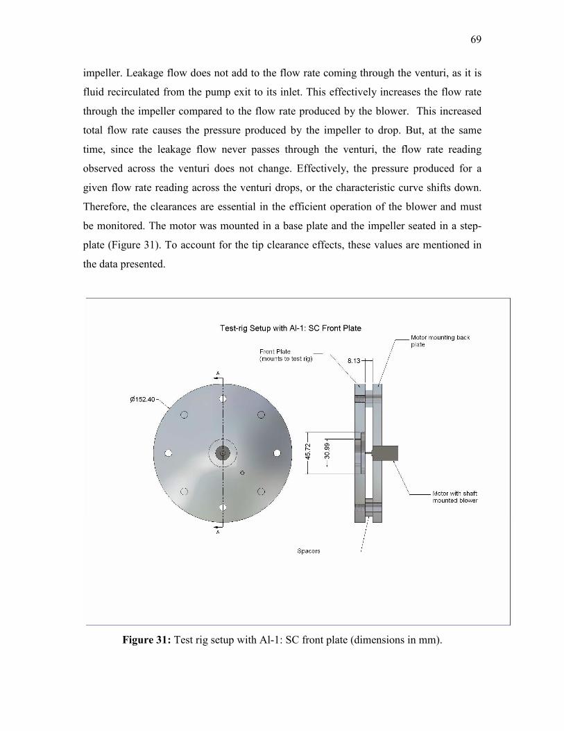
69
impeller. Leakage flow does not add to the flow rate coming through the venturi, as it is
fluid recirculated from the pump exit to its inlet. This effectively increases the flow rate
through the impeller compared to the flow rate produced by the blower. This increased
total flow rate causes the pressure produced by the impeller to drop. But, at the same
time, since the leakage flow never passes through the venturi, the flow rate reading
observed across the venturi does not change. Effectively, the pressure produced for a
given flow rate reading across the venturi drops, or the characteristic curve shifts down.
Therefore, the clearances are essential in the efficient operation of the blower and must
be monitored. The motor was mounted in a base plate and the impeller seated in a step-
plate (Figure 31). To account for the tip clearance effects, these values are mentioned in
the data presented.
Figure 31: Test rig setup with Al-1: SC front plate (dimensions in mm).

70
Experimental Data
The initial blower was tested but the data were not at all in agreement with the
simulations. This was attributed to the decreased blade height that resulted from the
shrinkage during the Rapid Prototyping (RP) process. This brought out the point that
blower dimensions, especially the blade width, are not accurate due to certain limitations
of the RP process. A machined blower might be a future recommendation once the design
is finalized.
Blower size 65xz_26y had an average (three readings) shroud diameter ( )2D of "753.1 ,
and an average impeller inlet diameter ( )ind of "200.1 after machining. Two different
front plates were used as given below:
• Aluminum Plate # 1 with Small Clearances ( )SCAl :1−
Plate inlet diameter ( )plateind , = "212.1
Plate shroud diameter ( ) "792.1,2 =plated
• Aluminum Plate # 2 with Bigger Clearances ( )BCAl :2−
Plate inlet diameter ( )
plateind , = "212.1
Plate shroud diameter ( ) "914.1,2 =plated
Based on these values the radial clearances one gets are:
• "006.0=inletδ
• "020.0=shroudδ
for SCAl :1−
• "080.0=shroudδ
for BCAl :2−
Shroud clearance values for BCAl :2− are relatively high (Karassik et al. 2000) and
should affect the performance. For SCAl :1− plate the values are acceptable, but better
results can be expected on reducing these clearances. Results for these two plates are
given next (Figures 32 and 33). Electrical power consumption measured is shown in
Figure 34, with comparison to FLUENT simulations given in Figure 35.

71
0
100
200
300
400
500
600
700
800
900
1000
1100
1200
1300
0 20 40 60 80 100 120 140 160 180 200 220
Q (flow rate), L/min
de
l P
sta
t (P
res
su
re),
Pa
EXP: 65xz_26y@10k
EXP: 65xz_26y@15k
EXP: 65xz_26y@18k
EXP: 65xz_26y@20k
EXP: 65xz_26y@22k
Figure 32: Experimental performance curves for 65xz_26y blower with Al-2: BC plate.
0
100
200
300
400
500
600
700
800
900
1000
1100
1200
0 20 40 60 80 100 120 140 160 180 200 220
Q (flow rate), L/min
de
l P
sta
t (P
res
su
re),
Pa
EXP: 65xz_26y@10k
EXP: 65xz_26y @15k
EXP: 65xz_26y@18k
EXP: 65xz_26y@20k
Figure 33: Experimental performance curves for 65xz_26y blower with Al-1: SC plate.

72
0
1
2
3
4
5
6
7
8
0 25 50 75 100 125 150
Q (flow rate), L/min
We
lec (
Ele
ctr
ica
l P
ow
er)
, W
EXP: 65xz_26y@20k Al1: SC
EXP: 65xz_26y@20k Al2: BC
Figure 34: Experimental electrical power consumption curves for 65xz_26y blower with
different front plates.
m L Increasing;
m constant
0
100
200
300
400
500
600
700
800
900
1000
1100
1200
0 20 40 60 80 100 120 140 160 180 200 220
Q (flow rate), l/min
de
l P
sta
t (P
res
su
re),
Pa
FLU: 65xz_26y@20k
EXP: 65xz_26y@20k Al1: SC
EXP: 65xz_26y@20k Al2:BC
Figure 35: Comparison between performance curves for FLUENT, Al-1: SC, and Al-2:
BC front plates.

73
The difference in the performance due to the tip clearance is clearly indicated. The
performance curves shift left as the clearance values are increased. This is because
Lm& increases from zero for simulations to a finite value as the clearances increase. Hence
impeller totalm& increases and curve shifts left.
FLUENT over-predicts the performance as compared to experimental results (Figure 33).
Experimentally, with smaller clearances one gets a pressure rise of 921 Pa as compared to
a predicted value of 1030 Pa. This represents a percentage error of 11%. This might have
been acceptable but for the fact that at 921 Pa the blower is not meeting the design
requirements. The 11% difference can be accounted for by the leakage flow (to a small
extent), and by the over-prediction of pressure by the FLUENT model being used. This
can be caused by the wall function used, as mentioned earlier. The next logical step is to
use enhanced wall treatment approach which is more robust and accurate for flows with
high body force and swirl effects (FLUENT User’s Guide 2004).
Observations and Conclusions
Important conclusions that can be drawn from this section are:
• Tip clearance plays an important part in blower performance
• FLUENT predictions match qualitatively with the experimental results
• FLUENT model over-predicts the experimental results gotten with Al-1:SC
relatively small clearances plate by 11%
• Blower size 65xz_26y@20k does not meet the design requirements in terms of
pressure rise.
• FLUENT model needs to be modified to improve the match to the experimental
results
• Since blower size 65xz_26y@20k cannot meet the design specification a bigger
blower must be used.

74
ENHANCED WALL TREATMENT
The difference in the two wall treatments can be understood in terms of the non-
dimensional distance, +yµ
ρ τ yu ..= to the wall from the first grid cell. The wall function
formulation requires a 30≈+y while for enhanced wall treatment requires
1≈+y (FLUENT User’s Guide 2004). The FLUENT manual says that a higher +y is
acceptable as long as it is well inside the viscous sublayer ( ) 5 4 toy <+ . In the present
case, the +y values were kept in this range. The total number of grid cells was
approximately 150,000 and this is an order of magnitude higher than for the previous
wall function approach (14,000). Adaptive meshing available in FLUENT was used to
progressively refine the grid.
Enhanced Wall Treatment FLUENT Simulations for 65xz_26y@20k Blower
Simulation data for 65xz_26y@20k blower with the enhanced wall treatment are given
below (Figure 36). Also shown is the experimental curve. Predictions by the enhanced
wall treatment are conservative. The percentage error is less for the enhanced wall
treatment approach (Figure 37). Nonetheless, the blower size chosen is not appropriate to
get to the design point. Enhanced wall treatment will be used to determine a new size
estimate for the blower. Before that, a conservative estimate of blower efficiency is given
next.

75
0
200
400
600
800
1000
1200
0 50 100 150Q (flow rate), L/min
de
l P
sta
t (P
res
su
re),
Pa
10
20
30
40
50
60
70
80
90
100
FL
UE
NT
Eff
icie
nc
y (
ηF
LU)
%
EXP: 65xz_26y@20k Al1: SC
FLU Pressure: Enhanced Wall Treatment
FLU Efficiency: Enhanced Wall
Treatment
Figure 36: Performance comparison for 65xz_26y blower: Enhanced wall treatment –vs.
- experimental results with Al-1: SC front plate
0
200
400
600
800
1000
1200
1400
de
l P
sta
t (P
res
su
re),
Pa
Non-equil Wall: Y+ ~ 60
Non-equil Wall: Y+ ~ 30
Enhanced Wall: Y+ ~ 5
EXP: 65xz_26y@20k Al1: SC
Figure 37: FLUENT static pressure rise value for 65xz_26y blower for different wall
treatments and comparison with Al-1: SC experimental data.

76
Conservative Efficiency Estimates for 65xz_26y@20k Blower
Estimates of the different blower efficiencies, namely, FLUFLUHY ηη and , from FLUENT
(Equation 32), and blowerEXP ηη and from experiments (Equation 33) are given below.
Following relations are used:
sheet) data (from efficiencymotor Maximum
.
=
=
motor
elecmotorS WW
η
η &&
[37]
Table 6 shows these values for the 100 L/min flow rate case. For the simulations, the
efficiencies are based upon total flow rate, i.e. Lmm && + . For the measurements, Lm& is not
known and only m& is used in the calculation, hence the flow rate in the impeller is
undetermined for the measurements. The blower specific speed at the design flow rate is
1096)(, =USsN (Equation 38)
[ ]( )( )
( ) 75.0
5.0
US
43
5.0
US
43
US
)(,ft
GPM.rpm1096
ft 8.425
GPM 4.26.rpm 20000
(ft)
)(GPM (rpm) ==
Δ=
tot
USsH
QNN
… [38]
Table 6: Blower efficiency estimates at design flow rate.
Blower Size 65xz_26y@20k
elecW& = 5.73 W
%69 =motorη (best, data sheet)
6.921=ΔEXPstatP Pa
SW& = 3.95 W
( )EXPstat mHg &Δ = 1.54 W

77
Table 6: continued.
( )FLUENTLtot mmHg && +Δ = 2.60 W
( )FLUENTLstat mmHg && +Δ = 1.48 W
FLUENTIW& = 2.7 W
%8.542.7
1.48 ==FLUη
%3.962.70
2.60 , ==FLUHYη
%275.73
1.54 ==EXPη
%393.95
1.54 ==blowerη
Figure 38: Efficiency values for pump with different specific speeds (Karassik et al.
2000, reprinted with permission of McGraw-Hill).

78
The present hydraulic efficiency predicted by FLUENT is 96.3% and it points to a well
designed blower. This high value can also be attributed to the fact that while calculating
totHΔ FLUENT assumes no leakage flow i.e. a volumetric efficiency of 100%, this may
lead to an over-prediction of the term ( )( )FLUENTLtot mmHg && +Δ used for efficiency
calculations. Assuming certain leakage percentage, the numerator in Equation 36 is
reduced and it affects a few percentage points on FLUHY ,η .
Nonetheless, the overall blower design is better than what is shown in Figure 38 but the
size needs to be changed to obtain the static pressure rise of 1000 Pa. This is given next.
Exact measurement of shaft power ( )SW& using rotary transducers, to verify the efficiency
values, can be part of any future work. This should consolidate the claim that the blower
design is good.
Resizing of Blower Using Enhanced-wall Treatment
Blower simulations were redone for different sizes using the enhanced wall treatment
approach. Since the overall blower efficiency is high, the simulation was done only at the
design flow rate of 100 L/min. Table 7 shows the results.
Table 7: Static pressure values for different sized blowers at design flow rate.
Blower Size ( )PastatPΔ ( )W IW&
65xz_26y 884.0 2.9
67xz_26y 923.0 2.8
68xz_26y 966.4 3.0
70xz_28y 1043.0 3.4
79
Since the results are under-predicted using the enhanced wall treatment approach, blower
size 68xz_26y seems the most appropriate. However, to allow for a small margin of
safety, it was decided to use the70xz_28y. The blower will produce more than 1000 Pa
when running at 20000 rpm. The rpm can be lowered to obtain the required pressure rise.

80
EXPERIMENTAL VALIDATION FOR 70XZ_28Y@20K BLOWER
The test rig was kept the same as for the previously tested blower. After machining, the
blower70xz_28y had an average (three readings) shroud diameter ( )2D of "888.1 , and an
average impeller inlet diameter ( )ind of "200.1 . A single front plate was used this time:
Aluminum Plate # 2 with Bigger Clearances ( )BCAl :2− . Since the impeller diameter is
bigger, the overall assembly had tighter clearances.
• "006.0=inletδ same as earlier case
• "013.0=shroudδ for BCAl :2− compared to "020.0 for SCAl :1−
Results
Experimental results are presented in Figure 39 and experimental electrical power
consumption in Figure 40. The experimental efficiency ( )EXPη value is shown after that
(Figure 41). The definition uses only the static head and ignores the velocity head for
efficiency calculations. It is also based upon the electrical power provided to the motor
and as such is the product of the blower and motor efficiency (Equation 33). It is a more
realistic estimate of performance.

81
0
200
400
600
800
1000
1200
1400
0 20 40 60 80 100 120 140 160 180 200 220
Q (flow rate), L/min
de
l P
sta
t (P
res
su
re),
Pa
EXP: 70xz_28y@15k
EXP: 70xz_28y@18k
EXP: 70xz_28y@20k
FLU: Enhanced Wall @20k
Figure 39: Experimental performance curve for 70xz_28y blower with Al-2: BC plate.
0
2
4
6
8
10
0 20 40 60 80 100 120 140 160
Q (flow rate), L/min
Ele
ctr
ica
l P
ow
er
(Wele
c),
W
EXP: 70xz_28y@15k
EXP: 70xz_28y@18k
EXP: 70xz_28y@20k
Figure 40: Experimental electrical power consumption curves for 70xz_28y blower with
Al-2: BC front plate.

82
0
10
20
30
40
0 20 40 60 80 100 120 140 160 180 200 220
Q (flow rate), L/min
Ex
pe
rim
en
tal E
ffic
ien
cy
(η
EX
P)
%
EXP: 70xz_28y@15k
EXP: 70xz_28y@18k
EXP: 70xz_28y@20k
Figure 41: Experimental efficiency ( )EXPη curves for 70xz_28y blower with Al-2: BC
front plate.
Conservative Efficiency Estimates for 70xz_28y@20k Blower
An estimate of the two different blower efficiencies, namely, FLUFLUHY ηη and , is given
below (Table 8). The blower specific speed at the design flow rate is
932)(, =USsN (Equation 39) gives the efficiency values:
[ ]( )( )
( ) 75.0
5.0
US
43
5.0
US
43
US
)(,ft
GPM.rpm932
ft 3.528
GPM 4.26.rpm 20000
(ft)
)(GPM (rpm) ==
Δ=
tot
USsH
QNN [39]

83
Table 8: Blower efficiency estimates at design flow rate .
Blower Size 70xz_28y@20k
elecW& = 7.0 W
%69 =motorη (best, data sheet)
EXPstatPΔ = 1111 Pa
SW& = 4.83 W
( )EXPstat mHg &Δ = 1.85 W
( )FLUENTLtot mmHg && +Δ = 3.23 W
( )FLUENTLstat mmHg && +Δ = 1.74 W
FLUENTIW& = 3.3 W
%7.523.3
1.74 ==FLUη
%8.973.3
3.23 , ==FLUHYη
%5.267.0
1.85 ==EXPη
%3.384.83
1.85 ==blowerη
Value of FLUHY ,η is high. Further, while calculating totHΔ FLUENT assumes no leakage
flow i.e. a volumetric efficiency of 100%, this may lead to an over-prediction of the term
( )( )FLUENTLtot mmHg && +Δ used for efficiency calculations. Further, at 20000 rpm the value
of FLUHY ,η is higher implying less separation and viscous losses.

84
Observations and Conclusions
Important observations from this section are given below:
• Blower size 70xz_28y running at 20000 rpm produces a static pressure rise of
1110 Pa experimentally, with the clearances as given by Al-2: BC front plate
• Blower efficiency is more than 38%. The exact value can only be determined by
making shaft torque measurements and total head rise measurements across the
blower.
• FLUENT model with enhanced wall treatment shows blower 70xz_28y rotating at
20000 rpm producing about 10% more head than the design requirements of 1000
Pa. This shows that a lower rpm value can be used; this is tested for the final
prototype
• Controlling tip clearances is important, but a clearance at the blower inlet of
"006.0=inletδ and on the shroud of "013.0=shroudδ work fine. For the final
prototype, inletδ is kept "009.0 and "012.0at shroudδ . This had to be done as the
final prototype was made out of Rapid Prototype (RP) material (plastic polymer)
and controlling tolerances with plastic is difficult.
• Maximum liquid pump efficiency values, as given in Figure 38, can not be
directly applicable to the present case but can only provide a benchmark
• Using a higher efficiency motor, a custom made brushless D.C motor, can help
bring down the electrical power ( )elecW& consumption.
• From the CFD point of view, enhanced wall function, with finer grid resolution,
gives better results as compared to non-equilibrium wall function approach.
• Still higher static pressure rise can be achieved by converting the large dynamic
head available at the blower exit. This can be done using a vaned stator or volute
diffuser. Simulations and experiments were carried out using one such vaned
diffuser, but no significant gain was observed.

85
FINAL BLOWER PROTOTYPE: DESIGN AND TESTING
Prototype Design Setup: Blower 70xz_28y with inletδ = "009.0 and shroudδ = "012.0
For the final prototype the entire blower assembly was rapid prototyped. This was done
keeping in mind the weight issues. Figure 42 shows the assembly. The overall diameter
of the top diffuser plate is "5.3 . Engineering drawings for the blower are given in
Appendix C.
Figure 42: Final blower prototype test setup.
The metallic spacers have been removed; instead the diffuser plate has vanes. These
vanes were designed to serve both as a support structure and for pressure recovery.
Despite repeated testing and design modification, no pressure gain was observed.
Nonetheless, these were retained to act as spacers between the top and the bottom halves
of the diffuser plate, and also to point towards a future possibility.

86
The tip clearances had to be controlled precisely. As the final prototype was fabricated
out of a plastic-type polymer, it was difficult to accurately control the dimensions.
Nonetheless, the tolerances were kept as tight as possible. Following values were used:
• Impeller diameter average ( )2D of "888.1
• Average impeller inlet diameter ( )ind of "200.1
• Front plate inlet diameter ( )plateind , = "218.1
• Plate shroud diameter ( )plated ,2 = "912.1
The clearances one gets from these are:
• "009.0=inletδ
• "012.0=shroudδ
Even though the shroud inlet clearance is more than the previous test cases, it appears to
have no effect on the overall blower performance. The results given below show this
point.
Results
As expected, running the impeller at 20000 rpm produces higher pressure rise than
needed. At 18000 rpm the pressure produced is 900 Pa and at 20000 rpm the pressure rise
is about 1150 Pa. Since pressure goes as 2Ω , to produce 1000 Pa the rpm should be
around 19000 rpm. Data tables are shown in Appendix D. Reducing the rpm also reduces
the electrical power consumption from 7 W to 6.2 W. At 19200 rpm FLUENT with
enhanced wall treatment gives pressure rise value of Pa 3.955=Δ statP . The pressure rise
value measured experimentally is 1021 Pa. The percentage under-prediction is less than
6%. This is good and it establishes faith in the CFD model being used. Figure 43 shows
the experimental performance curves at different rpm. Electrical power consumption,
measured experimentally is given in Figure 44, and Figure 45 shows the experimental
efficiency values at different rpms. Experimental efficiency value for original hand-held
vacuum system is also given. It shows a significant improvement.
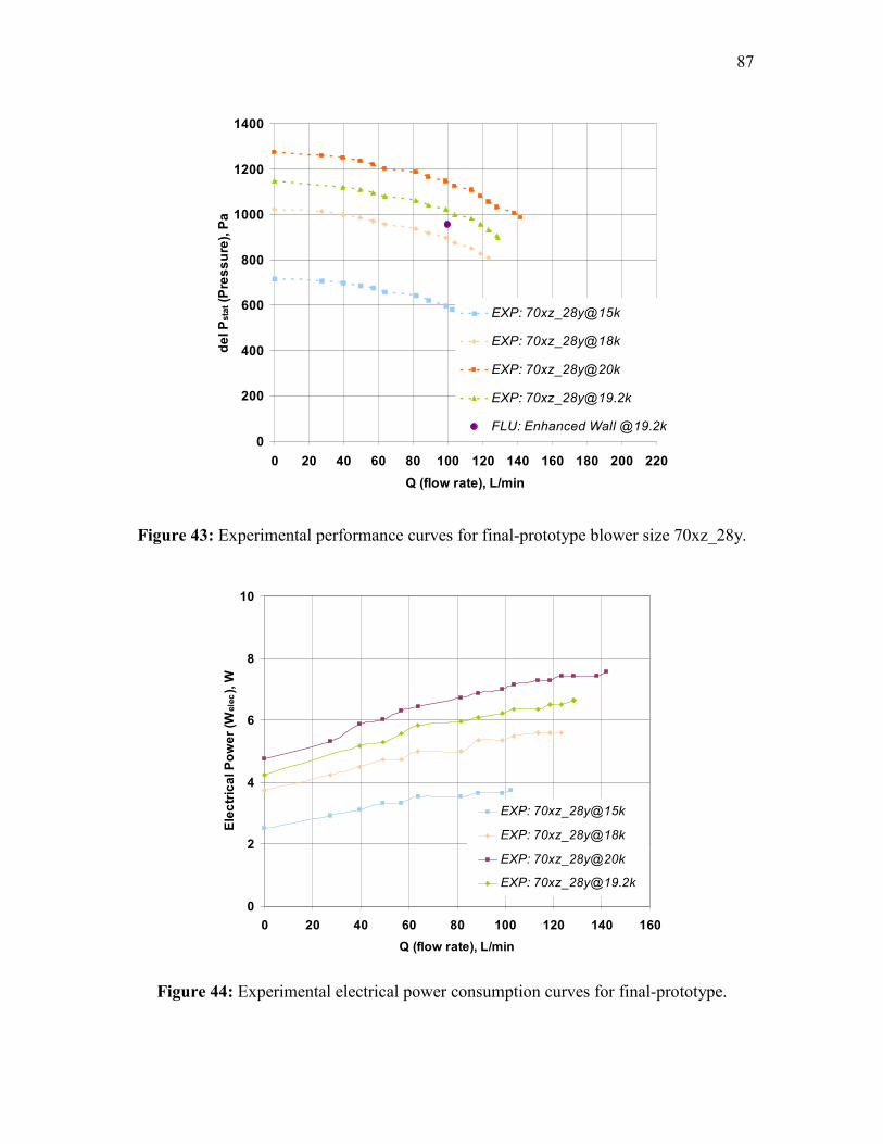
87
0
200
400
600
800
1000
1200
1400
0 20 40 60 80 100 120 140 160 180 200 220
Q (flow rate), L/min
de
l P
sta
t (P
res
su
re),
Pa
EXP: 70xz_28y@15k
EXP: 70xz_28y@18k
EXP: 70xz_28y@20k
EXP: [email protected]
FLU: Enhanced Wall @19.2k
Figure 43: Experimental performance curves for final-prototype blower size 70xz_28y.
0
2
4
6
8
10
0 20 40 60 80 100 120 140 160
Q (flow rate), L/min
Ele
ctr
ica
l P
ow
er
(Wele
c),
W
EXP: 70xz_28y@15k
EXP: 70xz_28y@18k
EXP: 70xz_28y@20k
EXP: [email protected]
Figure 44: Experimental electrical power consumption curves for final-prototype.

88
0
10
20
30
40
0 20 40 60 80 100 120 140 160 180 200 220
Q (flow rate), l/min
ηE
XP
EXP: 70xz_28y@15k
EXP: 70xz_28y@18k
EXP: 70xz_28y@20k
EXP: [email protected]
EXP: [email protected]
Figure 45: Experimental efficiency ( )EXPη values for final-prototype 70xz_28y.
The specific speed of the blower running at 19200 rpm is 965 (Equation 40). Results are
given below and the efficiency estimates given in Table 9.
• =Δ statP 1021 Pa from [email protected] measured experimentally
• =Δ (FLUENT) statP 955 Pa from enhance wall function approach.
• Percentage under-prediction %6<
[ ]( )( )
( ) 75.0
5.0
US
43
5.0
US
43
US
)(,ft
GPM.rpm965
ft 2.478
GPM 4.26.rpm 20000
(ft)
)(GPM (rpm) ==
Δ=
tot
USsH
QNN
… [40]

89
Table 9: Efficiency estimates for final prototype blower at design flow rate.
Blower Size [email protected]
elecW& = 6.23 W
%69 =motorη (best, data sheet)
EXPstatPΔ = 1021 Pa
SW& = 4.30 W
( )EXPstat mHg &Δ = 1.7 W
( )FLUENTLtot mmHg && +Δ = 2.92 W
( )FLUENTLstat mmHg && +Δ = 1.60 W
FLUENTIW& = 3.0 W
%3.533.0
1.60 ==FLUη
%3.973.0
2.92 , ==FLUHYη
%3.276.23
1.7 ==EXPη
%5.394.30
1.7 ==blowerη
From Figure 45, the efficiency improvement observed over the original 100xz_100y
system is more than 2X. This can be attributed to the better customization of blower size
to meet the design condition, and a higher efficiency motor that was used. The blower
certainly outperforms the efficiency values given in Figure 38.

90
SUMMARY AND CONCLUSIONS
Design, development, and testing of blowers for future aerosol applications were carried
out. Designing a blower to meet 100 L/min of flow rate and a static pressure rise of 1000
Pa was challenging. Lack of literature for such portable applications and dearth of
commercially available blowers to meet such low flow rate and pressure rise values made
the research necessary. A top-down design approach was adapted and it included
deciding the design objectives, selecting a blower type, designing a blower and testing
and validation. During the course of the study, the applicability of computational fluid
dynamics (CFD) to turbomachine design was established. Incorporating CFD into the
design process shortens the design cycle and adds a new dimension allowing the
visualization of flow field within the impeller.
Major findings from the study are given below:
• Maximum overall efficiency considerations established the blower type to be a
centrifugal impeller
• Optimum blower performance pointed towards a high rpm blower. Overall the
trend supported faster, smaller blowers.
• At high rpm values the blower static head cannot be ignored. High velocity head
adds to the overall efficiency. At the same time, the kinetic energy is not utilized
since the blower exhausts to the atmosphere.
• The approach towards blower design, adopted in the literature, is the modification
of an existing design rather than designing from base zero.
• Hand held vacuum systems, being battery operated, have blowers that are the
product of good engineering design. One such blower was used as a base-design
• CFD package, FLUENT, allowed the non-traditional scaling to be performed. A
blower 70% scaled in the ZX and directions and 28% scaled in Y running at
19,200 rpm was found to be the most appropriate

91
• Blower size 70xz_28y running at 19,200 rpm produces a static pressure rise of
1021 Pa
• It was found that the use of standard wall function approach (non-equilibrium
wall functions) over predicted the static pressure rise.
• FLUENT results allowed the blade height to be incorporated into the traditional
fan scaling equations. This lead to modified fan scaling laws. These relationships
are only from the simulated data and need to be modified.
• Finer grid resolution with the enhance wall function approach gave acceptable
agreement between simulations and experiments.
• Tip clearance, especially at the impeller inlet and shroud surfaces, significantly
affect blower performance
• Hydraulic efficiency value ( ),HY FLUη , based on the total head values given by
FLUENT is 98.12% at 19200 rpm.
Important inferences that can be drawn are:
• Design approach based on modifying an initial base-design is effective in meeting
the design requirements.
• CFD shortens the entire design process allowing the analysis of different scaling
cases with relative ease.
• Maximum liquid pump efficiency values, as given in Figure 38, may not be
directly applicable for the present case. In the absence of such charts for air
blowers, Figure 38 acts as a good benchmark
• Efficiency values for smaller blowers tend to reduce due to scale effect. CFD
overcomes this limitation by allowing non-traditional scaling.
• From the CFD point of view, enhanced wall function, with finer grid resolution,
gives better results as compared to non-equilibrium wall function approach.
• Controlling tip clearances is important for better performance
• Still higher static pressure rise can be achieved by converting the large dynamic
head available at the blower exit. This can be done using a vaned stator or volute
diffuser. This won’t affect the overall efficiency value.

92
RECOMMENDATIONS FOR FUTURE WORK
The work on this project is by no means complete. Designing and performance
improvement of air blowers for future aerosol samplers can go a long way. One probable
area is to establish overall efficiency versus specific speed graphs at different flow rates.
Another significant area is experimentally determining the overall blower efficiency
values. This can be done by measuring the shaft torque values using rotary transducers or
other such devices. For calculating efficiency values in this thesis, total head values
predicted by FLUENT were used. Even though, pressure predictions from FLUENT were
within acceptable error range, there is no way to validate the total head rise values given
by FLUENT. Experimental test-rig needs to be modified to be able to measure total head
change across the impeller. This will allow overallη to be determined and compared with
Figure 36 values. This will validate the performance improvement in the blower.
Clearance control on the impeller inlet and shroud affects performance significantly. For
any future prototypes, these values need to be controlled precisely. A recommendation
would be using aluminum front plate for better dimensional control. Final prototype was
made using plastic type resin and maintaining the precise tolerances on these was
difficult due to low machinability, moisture absorption, and temperature variations in the
surroundings.
Another area that can produce great performance level improvements is having a better
efficiency motor. A custom made D.C. brushless motor with high motor efficiency values
can go a long way in bringing down the D.C. power consumption. Looking into this
domain can be a possible next step.

93
REFERENCES
Anderson, H. H. (1980). Prediction of Head, Quantity, and Efficiency in Pumps The
Area Ratio Principle. Performance Prediction of Centrifugal Pumps and
Compressors, ASME. 1980, 201 211
Black, R. (2002). Development of the Wet Walled Cyclone Collector for the Joint
Biological Point Detection System, Presentation to the 2002 Scientific Conference on
Obscuration and Aerosol Research, Edgewood, MD.
Balje, O. E. (1962). A Study on Design Criteria and Matching of Turbomachinery, ASME
Journal of Engineering for Power. January, 83–102, 103–114.
Bleier, Frank, B. (1997). Fan Handbook: Selection, Application, and Design, McGraw
Hill, New York.
Cartwright, W. G. (1977). Specific Sped as a Measure of Design Point Efficiency and
Optimum Geometry for a Class of Compressible Flow Turbomachines, Scaling for
Performance Prediction in Rotodynamic Machines, Institution of Mechanical
Engineers, New York, 139–145
Engeda, A. (1995). Correlation and Prediction of Efficiency of Centrifugal Pumps due to
Tip Clearance Effects. Proc. of Institute of Mechanical Engineers. Vol. 20. 111–114
ERCOFTAC Best Practice Guidelines for Industrial Computational Fluid Dynamics
version 1 (2000). European Research Community on Flow, Turbulence, and
Combustion
European Commission Report (2001) Study on Improving the Energy Efficiency of
Pumps, February 2001 AEAT-6559/ v 5.1
FLOW-DYNE Engineering, Inc., Fort Worth, URL: http://www.flow-dyne.com.
Accessed August, 2004.
FLUENT 6.1.22. (2004). FLUENT Inc, Lebanon, NH
FLUENT User’s Guide Version 6.1.22. (2004). FLUENT, Inc, Lebanon, NH.
GAMBIT 2.1 User’s Guide (2004). FLUENT, Inc, Lebanon, NH
General Dynamics, Armament and Technical Products (2004). Joint Biological Point
Detection System (JBPDS), URL: http://www.gdatp.com/Products/PDFs/JBPDS.pdf

94
Graf, E. (1993). Analysis of Centrifugal Impeller BEP and Recirculating Flows:
Comparison of Quasi-3D and Navier-Stokes Solutions. Pumping Machinery – 1993.
FED – Vol. 154, ASME, 1993, 235 – 245.
Gülish, J. F., Favre, J. N., and Denus, K. (1997). An Assessment of Pump Impeller
Perfor-mance Predictions by 3D-Navier-Stokes Calculations. 1997 ASME Fluids
Enginee-ring Division Summer Meeting. Paper FEDSM97 – 3341, June 1997
Haglund, John S. and McFarland, Andrew R. (2004). A Circumferential Slot Virtual
Impactor, Aerosol Sci. Technology. 38:664 – 674.
Halstead, C. (2004). Fan Selection –A Practical Guide. Intern. Conf. on Fans, The Fluid
Machinery Group of the Institution of Mechanical Engineers, London 283 – 296
Han, Hai, Yokoyama, Yoichi, Konno, Brad M. (2002). Recent Developments and
Applications in CFD for Turbomachinery, 4th International Conference on Pumps
and Fans (4th
ICPF), Tsinghua University, Beijing
Hydraulics Institute, URL: http://www.pumps.org. Accessed January, 2005.
Inventor Professional 8 (2002), Autodesk Inc, San Rafael, CA
Isaguirre, Refugio R. (2004). An Experimental Study of Linear Slot Circumferential
Virtual Impactors for use in Continuous Bioaerosol Concentration, M.S. Thesis,
Texas A&M University, College Station
Japikse, David, Marscher, William D., Furst, Raymond B. (1997). Centrifugal Pump
Design and Performance, Concepts ETI, Inc.
Karassik, Igor J., Messina, Joseph P., Cooper, Paul, Heald Charles C. (2000). Pump
Handbook, McGraw Hill Professional, New York, 3rd
ed.
Katsanis, T. (1991). Quasi-Three-Dimensional Full Analysis in Turbomachines: A Tool
for Blade Design. Numerical Simulations in Turbomachinery, FEF – Vol. 120,
ASME, 1991, 57 – 64
Koh, C. P., Chan, W. K, Ng, B. T. H, Li, H. D. (1999). Design and Investigation of Flow
Field in a Centrifugal Blood Pump. ASME, Bioengineering Division. BED, Vol. 42,
1999, 167 – 168.

95
Lakshminarayana, B. (1991). An Assessment of Computational Fluid Dynamic
Techniques in the Analysis and Design of Turbomachinery – The 1990 Freeman
Scholar Lecture. J. of Fluids Engineering, Vol. 113: 315 – 352
Launder, B. E., and Spalding. D. B. (1972) Lectures in Mathematical Models of
Turbulence. Academic Press, London.
Lelkes, A. (2004). Novel Concepts for Improved Brushless Fan Motors. Intern. Conf. on
Fans, The Fluid Machinery Group of the Institution of Mechanical Engineers,
London 73 – 84
Mann, D. (2004). Fan Technology – Evolutionary Potential and Evolutionary Limits.
Intern. Conf. on Fans, The Fluid Machinery Group of the Institution of Mechanical
Engineers, London 225 – 235
Moncla, B. (2004). Personal communication, Aerosol Technology Laboratory, Texas
A&M University, College Station.
Pope, Stephen B. (2001). Turbulent Flows, Cambridge University Press, Cambridge.
Sabersky, R., and Acosta, A. J. (1966). Fluid Flow, Macmillan.
Tallgren, J. A., Sarin, D. A., and Sheard, A. G. (2004). Utilization of CFD in
Development of Centrifugal Fan Aerodynamics. Intern. Conf. on Fans, The Fluid
Machinery Group of the Institution of Mechanical Engineers, London 99 – 118
Thakur, Siddharth, Lin Wanlai, and Jeffrey Wright. (2002). Prediction of Flow in
Centrifugal Blower Using Quasi-Steady Rotor–Stator Models. J. of Eng. Mechanics,
October, 1039–1049
Tennekes, H. and Lumley, J. L. (1997). A First Course in Turbulence, MIT Press Design
Department, Cambridge, Massachusetts.
Turton, R. K. (1984). Principles of Turbomachinery, E. & F. N. Spon, New York.
Tuzson, John. (2000). Centrifugal Pump Design, A Wiley-Interscience publication, John
Wiley & Sons, Inc.
Wood, G. M., Welna, H. and Lamers, R. P. (1965). Tip Clearance Effects in Centrifugal
Pumps. ASME Tran., 85
Yakhot, V. and Orszag, S. A. (1986). Renormalization Group Analysis of Turbulence: I.
Basic Theory. Journal of Scientific Computing, 1(1):1-51

96
APPENDIX A
VENTURI CALIBRATION CHART
The calibration chart provided by the venturi company (FLOW-DYNE Engineering, Inc)
is given in Figure A-1. A sample calculation follows below.
Data Reduction
In using venturi for measuring flow rates, it is necessary to take 3 measurements pertinent
to flow condition. These are: 1) the inlet static pressure; 2) the inlet total temperature of
the flow media; and 3) the static pressure differential between the throat and the inlet. To
obtain the 100 L/min volume flow rate the following conditions are chosen:
Table A-1: Values chosen for mass flow calculation.
Throat diameter ( )2D "25.0
Inlet Static Pressure ( )1P 14.7 psia
Metering differential ( )PΔ 6” WC = 0.217 psia
Inlet Temperature ( )1OT RF oo 53474 =
01475.07.14
217.0
1
==ΔP
P. Project a horizontal line thru 01475.0
1
=ΔP
P on the air-curve
(Figure A-1).At the point where this line intersects the curve "25.02 =D , drop a vertical
line to the 1
1
P
TW Oscale and read 4.0
1
1 ≈P
TW O. Then solve for flow rate:
4.01
1 ≈P
TW O; minkg 11542.0minlbm 25445.0
534
7.144.04.0
1
1 ====OT
PW . This is
converted to volume flow rate using an air density value of 3mkg 17.1=airρ to get a
flow rate of 98.7 L/min. Manometer range is selected by back calculating the pressure
differential for the maximum flow rate expected.

97
Figure 46: Venturi calibration chart.

98
APPENDIX B
MOTOR DATA SHEETS
Brushless D.C. motors available from MicroMo Electronics (http://www.micromo.com) used
as blower drive. Data charts for the motor used, B024 2036 is given in Figure B-1. The
maximum motor efficiency value ( )motorη used in the thesis is referenced from these data
sheets.
Data sheets for the other motor, B024 1628 mentioned in the thesis can be obtained directly
from the homepage of MicroMo Electronics.

99
Figure B-1: B024 2036 motor data sheet.

100
APPENDIX C
70xz_28y Final Blower Prototype Drawings
Figure C-1: Blade dimensions (mm) for 70xz_28y final prototype.

101
Figure C-2: 70xz_28y final prototype dimensions (mm).

102
APPENDIX D
SAMPLE DATA SHEETS
Sample data sheet for the final prototype blower 70xz_28y running at 19,200 rpm is given
below (Table D-1). The nomenclature used is given below:
• o534=T R
• 7.14=atmP psi
• =ΔP Pressure difference across venturi ( )WC"
• ( )( )psi
psi
atmP
PY
Δ= Y-axis value on venturi chart
• =X X-axis intercept on venturi chart
• ( ) = minlbm m& mass rate from flow chart
• 3mkg 7.1=airρ
• ( )minL Q = flow rate calculated from (lbm/min) m&
• (Pa) statP = suction pressure at blower inlet
• V (V)= Voltage supplied to power supply
• I (Amp)= Current drawn by motor
• ( )W elecW& = Electrical power given to motor =V.I
• ( )W hydraulicW& = Hydraulic power generated by blower ( )statPQ.=
• EXPη

103
Table D-1: Sample data sheet for final prototype blower at design rpm.
Blower 70xz_28y @ 19200rpm
PΔ Y X m& Q ( )Pa statP V I ( )W elecW& ( )W hydraulicW& EXPη
0 0.00000 0 0.00 0 1145.8 26.5 0.16 4.24 0 0.00
0.5 0.00123 0.11 0.07 - - - - - - -
1 0.00246 0.16 0.11 39.5 1120.9 26.5 0.195 5.1675 0.74 14.27
1.5 0.00369 0.2 0.13 49.3 1110.9 26.5 0.2 5.3 0.91 17.24
2 0.00492 0.23 0.15 56.7 1096.0 26.5 0.21 5.565 1.04 18.63
3 0.00737 0.258 0.16 63.6 1081.0 26.5 0.22 5.83 1.15 19.67
4 0.00983 0.33 0.21 81.4 1061.1 26.5 0.225 5.9625 1.44 24.15
5 0.01229 0.36 0.23 88.8 1041.2 26.5 0.23 6.095 1.54 25.29
6 0.01475 0.4 0.25 98.7 1021.3 26.5 0.235 6.2275 1.68 26.97
7 0.01720 0.42 0.27 103.6 996.4 26.5 0.24 6.36 1.72 27.05
8 0.01966 0.46 0.30 113.5 981.4 26.5 0.24 6.36 1.86 29.19
9 0.02212 0.48 0.31 118.4 956.5 26.5 0.245 6.4925 1.89 29.08
10 0.02458 0.5 0.32 123.3 931.6 26.5 0.245 6.4925 1.92 29.50
11 0.02703 0.52 0.33 128.3 906.7 26.5 0.25 6.625 1.94 29.26
11.04 0.02713 0.521 0.33 128.5 896.7 26.5 0.25 6.625 1.92 29.00

104
VITA
Name: Raman Chadha
Email: [email protected]
Address: Department of Mechanical Engineering
Texas A&M University
Mail Stop 3123
College Station, Texas 77843-3123
Education: M.S. Mechanical Engineering (December 2005)
Texas A&M University (http://www.tamu.edu)
College Station, Texas 77843-3123
B-En., Mechanical Engineering (May 2003)
IIT Kanpur (http://www.iitk.ac.in)
Kanpur, India
Work Experience: 06/04-12/05 Graduate Research Assistant
Aerosol Technology Laboratory
Mechanical Engineering Department
Texas A&M University
College Station, Texas 77843-3123
08/03-05/04 Teaching Assistant
Thermodynamics Fluid Analysis and Design
(MEEN-421)
Mechanical Engineering Department
Texas A&M University
College Station, Texas 77843-3123