Design of Frequency Selective Surface (FSS) for Mobile ...
68
1 Design of Frequency Selective Surface (FSS) for Mobile Signal Shielding By Mohammed T. Al Haddad Supervisor Dr. Talal F. Skaik A Thesis Submitted to the Islamic University Of Gaza for the Degree of Master in communication Engineering Department of Electrical Engineering The Islamic University Of Gaza – IUG Palestine January 2016
Transcript of Design of Frequency Selective Surface (FSS) for Mobile ...

1
Design of Frequency Selective Surface
(FSS) for Mobile Signal Shielding
By
Mohammed T. Al Haddad
Supervisor
Dr. Talal F. Skaik
A Thesis Submitted to the Islamic University Of Gaza for the Degree of
Master in communication Engineering
Department of Electrical Engineering
The Islamic University Of Gaza – IUG
Palestine
January 2016

2
Abstract
The purpose of this project is to design novel structures of frequency selective surfaces (FSS).
FSSs have been the subject of intensive investigation for their widespread applications in communication
and radar systems. For practical applications, it is desired to realize a FSS with miniaturized elements and
a stable frequency response for different polarizations and incident angles. But these features are difficult
to obtain through traditional designs.
The focus in this thesis was to shield the signals of mobile communications, and five FSS models have
been designed to achieve that based on 2D periodic arrays. The simulations are done using CST
Microwave Studio.
First design which is double square loop microstrip structure covered GSM900 and GSM1800
bands while the second design is a novel microstrip model that covered the bands GSM900, GSM1800
and LTE. The third design is similar to previous designs but with glass substrate to be suitable for wide
buildings, and the fourth model covers more bands including GSM900, GSM1800, 3G (UMTS) and LTE.
The last model is designed to be suitable to the outdoor applications and it is made from double wired net
joined with iron cylinders and it covers the bands GSM900, GSM1800 and 3G.
The simulation results showed good performance for scattering parameters for different
polarizations and also various incident angles.

3
Acknowledgement
First and foremost, I would like to express my gratitude and appreciation to my supervisor, Dr
Talal F. Skaik, for his patient guidance, encouragement, precious advice and suggestions through the
whole project. Also I like to thank Dr. Ammar Abu Hadrouss and Dr. Tamer Abu Foul for acceptance to
examine my thesis. I would also like to extend my sincere thanks to all colleagues in communication
group who gave me comprehensive knowledge during the past two academic years. Also I like to extend
my sincere thanks to my father and mother to moral support and encouragement before and during the
study period.
Finally, extend deep thanks and appreciation to my beloved family for their loving consideration
and continuous support , especially for my dear wife for all the support and care during the study period.

4
Table of contents
CHAPTER 1: INTRODUCTION ................................................................................................. 9
1.1 BACKGROUND ............................................................................................................................ 9
1.2 APPLICATIONS .......................................................................................................................... 10
1.3 GENERATIONS OF MOBILE COMMUNICATION SYSTEMS .................................................................... 11
1.3.1 First generation ................................................................................................................ 12
1.3.2 Second generation ........................................................................................................... 12
1.3.3 Third generation (3G) ...................................................................................................... 13
1.3.4 Fourth generation ............................................................................................................ 16
1.4 GLOBAL MOBILE SUBSCRIBERS AND MARKET SHARE BY TECHNOLOGY ................................................. 17
1.5 FREQUENCY BANDS OF GENERATIONS ........................................................................................... 17
1.5.1 Frequencies of GSM 900-1800 bands ............................................................................. 17
1.5.2 Frequencies of 3G bands ................................................................................................. 18
1.5.3 Frequencies of 4G Bands ................................................................................................. 19
1.6 THESIS OBJECTIVE ...................................................................................................................... 22
1.7 THESIS OVERVIEW ..................................................................................................................... 22
CHAPTER 2: FREQUENCY SELECTIVE SURFACE THEORY ........................................................ 23
2.1 THE RELEVANT CONCEPTS IN ELECTROMAGNETIC THEORY ................................................................ 23
2.2 FILTER GEOMETRIES AND EQUIVALENT CIRCUITS............................................................................ 24
2.3 STRIP GRATING FILTERS ............................................................................................................. 25
2.4 MESH FILTERS .......................................................................................................................... 27
2.5 CROSS-MESH FILTERS ................................................................................................................ 28
2.6 ANALYSIS OF MORE COMPLEX STRUCTURES................................................................................... 29
2.6.1 Square Loop FSS ............................................................................................................... 29
2.6.2 Jerusalem Cross................................................................................................................ 32
2.7 A BRIEF OF MOST COMMON FSS GEOMETRIES ............................................................................... 35
2.8 LITERATURE REVIEW .................................................................................................................. 36
CHAPTER 3: DESIGNS AND SIMULATIONS OF FREQUENCY SELECTIVE SURFACES.................. 38
3.1 INTRODUCTION ......................................................................................................................... 38
3.2 DESIGNS AND SIMULATIONS:....................................................................................................... 38
3.2.1 Goals of designs ............................................................................................................... 38
3.2.2 Simulation Software CST ................................................................................................. 38
3.3 BASICS OF THE DESIGNS.............................................................................................................. 38
3.4 BANDSTOP DOUBLE SQUARE LOOP FSS......................................................................................... 39

5
3.4.1 Structure of FSS ................................................................................................................ 39
3.4.2 Simulation results ............................................................................................................ 40
3.5 TRI BANDSTOP OPEN LOOP FSS WITH FR SUBSTRATE ...................................................................... 42
3.5.1 Structure of FSS ................................................................................................................ 42
3.5.2 Simulation results ............................................................................................................ 43
3.6 TRI BANDSTOP OPEN LOOP FSS WITH GLASS (PYREX) SUBSTRATE ...................................................... 47
3.6.1 Structure of FSS ................................................................................................................ 48
3.6.2 Simulation results ............................................................................................................ 49
3.7 QUAD BANDSTOP E_SHAPE FSS .................................................................................................. 52
3.7.1 Structure of FSS ................................................................................................................ 52
3.7.2 Simulation results ............................................................................................................ 54
3.7.3 The effect of changing the widths of elements.............................................................. 55
3.8 DUAL BANDSTOP DOUBLE WIRED SQUARE LOOP FSS ...................................................................... 56
3.8.1 Structure of FSS ................................................................................................................ 57
3.8.2 Simulation results ............................................................................................................ 58
CHAPTER 4: CONCLUSION .................................................................................................. 61
4.1 SUMMARY ............................................................................................................................... 61
4.1.1 First design (Bandstop double square loop FSS) ............................................................ 61
4.1.2 Second design (Tri bandstop open loop FSS with FR substrate) ................................... 61
4.1.3 Third design (Tri bandstop open loop FSS with glass (pyrex) substrate) ..................... 62
4.1.4 Fourth design (Quad bandstop E_shape FSS) ................................................................ 62
4.1.5 Fifth design (Dual Bandstop double wired square loop FSS) ........................................ 63
4.2 FUTURE WORK .......................................................................................................................... 63
REFERENCES ........................................................................................................................ 64
List of Figures
FIGURE 1.1: STRUCTURES OF FSS ................................................................................................................................ 10
FIGURE 1.2: MARSCHALS QUASI-OPTICAL FEED TRAIN ............................................................................................... 11
FIGURE 1.3: TIME DIVISION MULTIPLE ACCESS ........................................................................................................... 13
FIGURE 1.4: CODE DIVISION MULTIPLE ACCESS .......................................................................................................... 13
FIGURE 1.5: GLOBAL MOBILE SUBSCRIBERS AND MARKET SHARE BY TECHNOLOGY ................................................. 17
FIGURE 1.6: GSM (GROUP SPECIAL MOBILE) - GLOBAL SYSTEM FOR MOBILE COMMUNICATIONS - MOST POPULAR
STANDARD FOR PHONES IN THE WORLD. GSM 900 / GSM 1800 MHZ ARE USED IN MOST PARTS OF THE

6
WORLD: EUROPE, ASIA, AUSTRALIA, MIDDLE EAST, AND AFRICA. GSM 850 / GSM 1900 MHZ ARE USED IN THE
UNITED STATES, CANADA, MEXICO AND MOST COUNTRIES OF S. AMERICA ..................................................... 18
FIGURE 1.7 : FREQUENCIES SEPARATED BY GAP ......................................................................................................... 19
FIGURE 2.1: (A) PATCH ELEMENTS, (B) APERTURE ELEMENTS .................................................................................... 23
FIGURE 2.2: (A) ELECTRON IN FILTER PLANE UNDERGOES OSCILLATIONS DRIVEN BY SOURCE WAVE, (B) ELECTRON
CONSTRAINED TO MOVE ALONG WIRE CANNOT UNDERGO OSCILLATIONS...................................................... 24
FIGURE 2.3: IF THE E-FIELD IS PERPENDICULAR TO THE STRIPS THE FILTER SWITCHES BETWEEN STATES A AND B, IF
IT IS PARALLEL TO THE STRIP THE FILTER SWITCHES BETWEEN C AND D. .......................................................... 25
FIGURE 2.4: STRIP-GRATING FILTERS AND ITS EQUIVALENT CIRCUIT ......................................................................... 25
FIGURE 2.5: PLANE WAVE INCIDENT ON AN INDUCTIVE STRIP GRATING, FOR A CAPACITIVE STRIP GRATING
EXCHANGE THE INCIDENT ELECTRIC FIELD E FOR A MAGNETIC FIELD H ............................................................ 26
FIGURE 2.6: MESH FILTERS AND ITS EQUIVALENT CIRCUIT ......................................................................................... 28
FIGURE 2.7: CROSS-MESH FILTERS............................................................................................................................... 29
FIGURE 2.8: A) LAYOUT OF SQUARE LOOP ARRAYS, B) EQUIVALENT CIRCUIT ............................................................ 30
FIGURE 2.9: ANALYSIS OF SQUARE LOOP FSS .............................................................................................................. 30
FIGURE 2.10: EQUIVALENT CIRCUIT FOR SQUARE LOOP ............................................................................................. 31
FIGURE 2.11: JERUSALEM CROSS PERIODIC ARRAY ..................................................................................................... 33
FIGURE 2.12: EQUIVALENT CIRCUIT OF JERUSALEM CROSS ........................................................................................ 33
FIGURE 2.13: FREQUENCY RESPONSE OF JERUSALEM CROSS ..................................................................................... 33
FIGURE 2.14: JERUSALEM CROSS ETCHED IN DIELECTRIC SLAB .................................................................................. 34
FIGURE 3.1: A) DIMENSIONS OF SQUARE LOOP FSS, B) SIDE VIEW OF THE MODEL ................................................... 39
FIGURE 3.2: A) PERIODIC FSS, B) FSS MODEL WITH INCIDENT PLANE WAVE .............................................................. 40
FIGURE 3.3: SIMULATION RESULTS OF DUAL-BANDSTOP FSS FOR TM POLARIZATION .............................................. 41
FIGURE 3.4: SIMULATION RESULTS OF DUAL-BANDSTOP FSS FOR TE POLARIZATION................................................ 41
FIGURE 3.5: OVERALL VIEW OF THE UNIT CELL MODEL .............................................................................................. 42
FIGURE 3.6: A) DIMENSIONS OF TOP VIEW MODEL, B) SIDE VIEW OF THE MODEL .................................................... 43
FIGURE 3.7: PERIODIC CELLS ........................................................................................................................................ 44
FIGURE 3.8: SIMULATION RESULTS OF TRI-BANDSTOP FSS FOR TE POLARIZATION ................................................... 44
FIGURE 3.9: SIMULATION RESULTS OF TRI-BANDSTOP FSS FOR TM POLARIZATION .................................................. 45
FIGURE 3.10: TRANSMISSION BANDWIDTHS AT 900/1800 MHZ AND LTE BAND FOR TE POLARIZATION AT THETA=0
............................................................................................................................................................................ 46
FIGURE 3.11: TRANSMISSION BANDWIDTHS AT 900/1800 MHZ AND LTE BAND FOR TE POLARIZATION AT THETA=30
............................................................................................................................................................................ 46
FIGURE 3.12: TRANSMISSION BANDWIDTHS AT 900/1800 MHZ AND LTE BAND FOR TM POLARIZATION AT THETA=0
............................................................................................................................................................................ 47
FIGURE 3.13: TRANSMISSION BANDWIDTHS AT 900/1800 MHZ AND LTE BAND FOR TM POLARIZATION AT
THETA=30 ............................................................................................................................................................ 47
FIGURE 3.14: OVERALL VIEW OF THE UNIT CELL MODEL ............................................................................................ 48
FIGURE 3.15: A) DIMENSIONS OF TOP VIEW MODEL, B) SIDE VIEW OF THE MODEL .................................................. 48
FIGURE 3.16: SIMULATION RESULTS OF TRI-BANDSTOP FSS FOR TE POLARIZATION ................................................. 49

7
FIGURE 3.17: SIMULATION RESULTS OF TRI-BANDSTOP FSS FOR TM POLARIZATION ................................................ 50
FIGURE 3.18: TRANSMISSION BANDWIDTHS AT 900/1800 MHZ AND LTE BAND FOR TE POLARIZATION AT THETA=0
............................................................................................................................................................................ 51
FIGURE 3.19: TRANSMISSION BANDWIDTHS AT 900/1800 MHZ AND LTE BAND FOR TE POLARIZATION AT THETA=30
............................................................................................................................................................................ 51
FIGURE 3.20: TRANSMISSION BANDWIDTHS AT 900/1800 MHZ AND LTE BAND FOR TM POLARIZATION AT THETA=0
............................................................................................................................................................................ 52
FIGURE 3.21: TRANSMISSION BANDWIDTHS AT 900/1800 MHZ AND LTE BAND FOR TM POLARIZATION AT
THETA=30 ............................................................................................................................................................ 52
FIGURE 3.22: OVERALL VIEW OF THE UNIT CELL MODEL ............................................................................................ 53
FIGURE 3.23: A) DIMENSIONS OF TOP VIEW MODEL, B) SIDE VIEW OF THE MODEL .................................................. 53
FIGURE 3.24: PERIODIC CELLS ...................................................................................................................................... 54
FIGURE 3.25: SIMULATION RESULTS OF QUAD-BANDSTOP FSS FOR TE POLARIZATION............................................. 55
FIGURE 3.26: SIMULATION RESULTS OF QUAD-BANDSTOP FSS FOR TE POLARIZATION WITH VARYING THE
ELEMENTS WIDTH ............................................................................................................................................... 55
FIGURE 3.27: COMPARISON BETWEEN TE AND TM POLARIZATION ........................................................................... 56
FIGURE 3.28: DIMENSIONS OF TOP VIEW MODEL....................................................................................................... 57
FIGURE 3.29: PERIODIC SQUARE CELLS ....................................................................................................................... 58
FIGURE 3.30: SIMULATION RESULTS OF TRI-BANDSTOP FSS FOR TE POLARIZATION ................................................. 59
FIGURE 3.31: SIMULATION RESULTS OF TRI-BANDSTOP FSS FOR TM POLARIZATION ................................................ 59
FIGURE 3.32: TE AND TM POLARIZATION AT THETA=0 ............................................................................................... 60
FIGURE 3.33: TE AND TM POLARIZATION AT THETA=40 ............................................................................................. 60
List of Tables
TABLE 1.1: 2G / 3G CELLULAR WIRELESS DATA TRANSPORT TERMINOLOGY ............................................................. 15
TABLE 1.2: (A) WIMAX RELEASE 2.0 (802.16M) TECHNICAL SPECIFICATIONS, (B) LTE-ADVANCED TECHNICAL
SPECIFICATIONS ................................................................................................................................................. 16
TABLE 1.3: 3G UMTS FREQUENCY BANDS – FDD ........................................................................................................ 18
TABLE 1.4: FDD LTE BANDS AND FREQUENCIES .......................................................................................................... 20
TABLE 1.5: TDD LTE BANDS AND FREQUENCIES .......................................................................................................... 21
TABLE 2.1: A BRIEF OF MOST COMMON FSS GEOMETRIES AND ITS EQUIVALENT CIRCUITS...................................... 35
TABLE 3.1: DIMENSIONS OF THE DESIGN .................................................................................................................... 39
TABLE 3.2: -10 DB TRANSMISSION BANDWIDTHS AT 900/1800 MHZ FOR TM POLARIZATION ................................. 41
TABLE 3.3: -10 DB TRANSMISSION BANDWIDTHS AT 900/1800 MHZ FOR TE POLARIZATION................................... 42
TABLE 3.4: DIMENSIONS OF THE DESIGN .................................................................................................................... 43
TABLE 3.5: -10 DB TRANSMISSION BANDWIDTHS AT 900/1800 MHZ AND LTE BAND FOR TE POLARIZATION .......... 45
TABLE 3.6: : -10 DB TRANSMISSION BANDWIDTHS AT 900/1800 MHZ AND LTE BAND FOR TM POLARIZATION ....... 46

8
TABLE 3.7: DIMENSIONS OF THE DESIGN .................................................................................................................... 49
TABLE 3.8: -10 DB TRANSMISSION BANDWIDTHS AT 900/1800 MHZ AND LTE BAND FOR TE POLARIZATION .......... 50
TABLE 3.9 : -10 DB TRANSMISSION BANDWIDTHS AT 900/1800 MHZ AND LTE BAND FOR TM POLARIZATION ........ 51
TABLE 3.10: DIMENSIONS OF THE DESIGN .................................................................................................................. 54
TABLE 3.11: DIMENSIONS OF THE DESIGN .................................................................................................................. 57
TABLE 3.12: -10 DB TRANSMISSION BANDWIDTHS AT 900/1800 MHZ AND 3G BAND FOR TE POLARIZATION.......... 60
TABLE 3.13: -10 DB TRANSMISSION BANDWIDTHS AT 900/1800 MHZ AND LTE BAND FOR TM POLARIZATION ....... 60
TABLE 4.1: (DB) AT DESIRED FREQUENCIES AT THETA = .................................................................................. 61
TABLE 4.2: TABLE 1: (DB) AT DESIRED FREQUENCIES AT THETA = 45 .................................................................. 61
TABLE 4.3: (DB) AT DESIRED FREQUENCIES AT THETA = ................................................................................... 61
TABLE 4.4: (DB) AT DESIRED FREQUENCIES AT THETA = 3 ................................................................................ 62
TABLE 4.5: (DB) AT DESIRED FREQUENCIES AT THETA = ................................................................................... 62
TABLE 4.6: (DB) AT DESIRED FREQUENCIES AT THETA = 3 ................................................................................ 62
TABLE 4.7: (DB) AT DESIRED FREQUENCIES AT THETA = ................................................................................... 62
TABLE 4.8: (DB) AT DESIRED FREQUENCIES AT THETA = ................................................................................... 63
TABLE 4.9: (DB) AT DESIRED FREQUENCIES AT THETA = 3 ................................................................................ 63
9
Chapter 1: Introduction
1.1 Background:
Todaytheworldiswitnessingasignificantincreaseintheuseofmobiledevices,which
leadscompaniestoexpandmobilenetworkstoincludeallwalksoflifeincludingtheinstallation
ofmacrocellstoamplifythesignalswithinthebuildingsthemselves.
Some facilities contain sensitive electronic devices couldbe affected by these signals, suchas
labs,Inaddition,someofthebodiesandinstitutionswanttoisolatesomeplacescommunication
devicesforsecurityconsiderations,suchasprisons.
Moreover, some places prevent the use of mobile devices, such as intensive care rooms in
hospitals, and placesofworship. Jammersareused toachieve that, but theyneeda sourceof
energythatcancauseundesirableeffectsonsomeultra-sensitivedevices.
Othertechnologyusedtoachievethedesiredshieldingisfrequencyselectivesurface(FSS).
Afrequencyselective surface isa spatial electromagnetic filter includesatleastone frequency
selective layer made up of an array of electrically conductive elements (patch elements) or
apertureelementsetchedonadielectricsubstrate.
Theselectivesurfaceworksasbandpassorbandstopfilter.Thepatchelementarraybehavesas
abandstopfilterandtheapertureelementarrayactsasabandpassfilter.
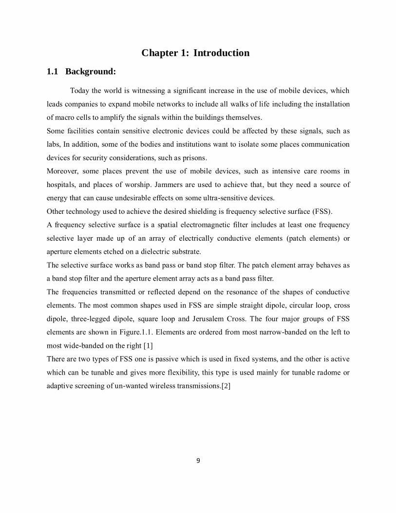
The frequencies transmitted or reflected depend on the resonanceof the shapesof conductive
elements.ThemostcommonshapesusedinFSSare simplestraightdipole,circularloop,cross
dipole, three-legged dipole, square loop and JerusalemCross.The four major groups of FSS
elementsareshowninFigure.1.1.Elementsareorderedfrommostnarrow-bandedontheleftto
mostwide-bandedontheright[1]
TherearetwotypesofFSSoneispassivewhichisusedinfixedsystems,andtheotherisactive
whichcanbetunableandgivesmoreflexibility,thistype isusedmainlyfortunableradomeor
adaptivescreeningofun-wantedwirelesstransmissions.[2]
10
Figure 1.1:structuresofFSS
1.2 Applications:
Frequencyselectivesurfacesareusedinawidevarietyofapplicationssuchasbelow:
Therealizationofreflectorantennasystemswhichenablestwoormorefeedstosharethe
sameparabolicmainreflectorsimultaneously.
Radome design, FSS used with a protective radome to reduce the radar cross section
(RCS)oftheenclosedantennaoutsideitsoperatingband.[3]
Makingpolarizers,forexample,circularpolarization(CP)areusedinradarapplications.
TheadvantagesofaCPoverlinearpolarization(LP)isthatithaslowersusceptibilityto
themulti-path,atmosphericabsorptionandreflectionseffects.[4]

11
To reduce the adjacent channel interference in the communication systems due to the
congestionoftheelectromagneticspectrum,severalFSSstructureslikedipole,Jerusalem
cross,ring,tripod,drossdipoleandsquareloophavebeendeveloped[5]
Filters for Earth Observation Remote Sensing Instruments by separating the scene
radiation into separate frequency channels [6].By providing frequency selective beam
splittinginthe feedtrainthusvastlyreducingthe sizeandmassof theantenna
systemandminimizethefilterinsertionloss[7]asshowninFigure1.2.1.
Figure 1.2:MARSCHALSquasi-opticalfeedtrain
One important application of selective surfaces is to shield the mobile signals for a
variety of reasons that would make clear later, the following is an overview of the mobile
networks
1.3 Generations of mobile communication systems
Thegenerationsofmobilecommunicationsystemsarepresentedheresincethemainapplication

12
in the current thesis is to use FSS to block mobile signals. Mobile phone network has been
historically divided into four generations, each generation has specific characteristics that
distinguishitfromotherEachgenerationisdifferentfromtheotherintermsoffrequency,data
rate, maximum number of users and the geographical area covered by the network. The
followingisabriefexplanationofeachgeneration.
1.3.1 First generation of the network appeared in the 1980s and started with
the advanced mobile phone service (AMPS) which has the below
features [8,9,10]: Basedonanalogcommunications
Supportonlyvoicetransmissions
Usefrequencydivisionmultipleaccess(FDMA)with30kHzforeachchannel
Thefrequencyisrangingfrom824MHzto894MHz
Two25MHzbandareallocated,oneforuploadfrequency(frommobileunittothebase
station)andotherfordownloadfrequency(frombasestationtothemobileunit)
1.3.2 Second generation appeared in the 1990s and has the below features
[11,12]: Basedondigitalcommunications
Voicecallsarebecomingclearerandthecommunicationsareencrypted
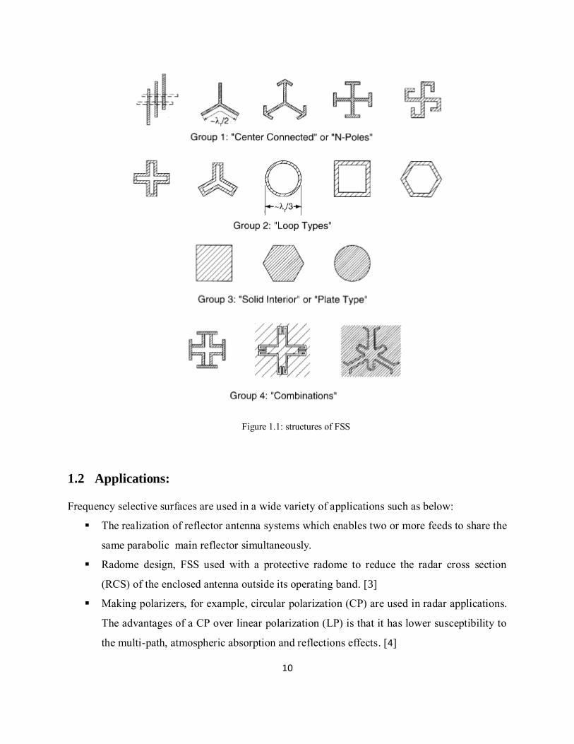
TheTimeDivisionMultipleaccess(TDMA)(Figure1.3) -basedGlobalSystem for
Mobile(GSM)systemandtheCodeDivisionMultipleAccess(CDMA)(Figure1.4)
–basedInterimStandard95 (IS-95)system.
Supportedbettervoiceandtexttransmissions.
Thefrequencybandsare900and1800MHz
TheGSMArchitectureisbasedonGaussianMinimumShiftKeying(GMSK)scheme
The GSM 900 system uses two 25-MHz bands for the uplink and downlink, and
within this spectrum200-KHz channelsareallocated.Theuplinkand downlinkare
separatedbya45-MHzspacing.GSM1800uses two75-MHzbands for theuplink
and downlink. Again 200-KHz channels are allocated within those bands and are
separatedbya95-MHzspacing.The1900-MHzsystemsusetwo60-MHzbandsfor
theuplinkanddownlinkusing200-KHzchannelswithin thosebandsand separated
13
by80-MHzspacing.
Figure 1.3:TimeDivisionMultipleaccess
Figure 1.4:CodeDivisionMultipleAccess[13]
1.3.3 Third generation (3G)
Thistechnologyhasgreatlyhelpedinthedevelopmentofwirelessservices,whichincluded
voice telephony, mobileInternet access, fixedwireless internetaccess, videocalls and mobile
TV.3Gusesservicesandnetworksthatcomplywiththe InternationalMobile
Telecommunications-2000 (IMT-2000) specifications.
Thefirst3GnetworkwaslaunchedinMay2001inatestreleaseasWidebandCodeDivision
MultipleAccess(WCDMA)technologyinJapan.ThefirstUniversalMobile

14
TelecommunicationsSystem(UMTS)(basedWCDMA)networkwaslaunchedinEuropein
December 2001.
The UMTS system,usedprimarilyinEurope,Japan,China(howeverwithadifferentradio
interface)andotherregionspredominatedby GSM 2G systeminfrastructure.Thecellphonesare
typicallyUMTSandGSMhybrids.Severalradiointerfacesareoffered,sharingthesame
infrastructure:
Theoriginalandmostwidespreadradiointerfaceiscalled W-CDMA.
The Time-Division Synchronous Code-Division Multiple-Access (TD-SCDMA) radio
interfacewascommercializedin2009andisonlyofferedinChina.
The latest UMTS release, High Speed PacketAccess (HSPA+), can provide peak data
ratesupto28 Mbit/sinthedownlinkand22 Mbit/sintheuplink.
UMTS networkusingthe CDMA2000 technology,firstofferedin2002inUSA,usedespecially
inNorthAmericaandSouthKorea, sharinginfrastructurewiththe IS-95 2Gstandard.Thecell
phonesaretypicallyCDMA2000andIS-95hybrids.[14]
3Gnetworkhasthebelowfeatures:
Widercoveragearea
Improvespectralefficiency
Greaternetworkcapacity
Moreservicesincludevideocallsandbroadbandwirelessdata
Dataratereached14.4Mb/sondownlinkand5.8Mb/sonuplink
2G/3GCellular terminologyisillustratedinTable1.1

15
Table 1.1:2G/3GCellularWirelessdatatransportterminology[15]
Transport
technology Description
Typical use/Data
transmission speed Pros/cons
TDMA
TimeDivisionMultiple
Accessis2Gtechnology
VoiceanddataUpto9.6kbps Lowbatteryconsumption,but
transmissionisone-way,anditsspeed
palesnextto3Gtechnologies
GSM
GlobalSystemforMobile
Communicationsisa2G
digitalcellphonetechnology
Voiceanddata.ThisEuropean
systemusesthe900MHzand1.8GHz
frequencies.IntheUnitedStatesit
operatesinthe1.9GHzPCS
band Upto9.6kbps
Populararoundtheglobe.Worldwide
roaminginabout180countries,but
GSM'sshortmessagingservice(GSM-
SMS)onlytransmitsone-way,andcan
onlydelivermessagesupto160
characterslong
GPRS
GeneralPacketRadioService
isa2.5Gnetworkthat
supportsdatapackets
DataUpto115kbps;theAT&T
WirelessGPRSnetworkwilltransmit
dataat40kbpsto60kbps
Messagesnotlimitedto160characters,
likeGSMSMS
EDGE
EnhancedDataGSM
Environmentisa3Gdigital
network
Data
Upto384kbps
Maybetemporarysolutionforoperators
unabletogetW-CDMAlicenses
CDMA
CodeDivisionMultiple
Accessisa2Gtechnology
developedbyQualcommthat
istransitioningto3G
AlthoughbehindTDMAinnumberof
subscribers,thisfast-growingtechnology
hasmorecapacitythanTDMA
W-CDMA
(UMTS)
WidebandCDMA(alsoknownasUniversalMobile
TelecommunicationsSystem--
UMTS)is3Gtechnology.On
November6,2002,NTT
DoCoMo,Ericsson,Nokia,
andSiemensagreedon
licensingarrangementsforW-
CDMA,whichshouldseta
benchmarkforroyaltyrates
Voiceanddata.UMTSisbeingdesignedtoofferspeedsofatleast
144kbpstousersinfast-moving
vehicles
Upto2Mbpsinitially.Upto10Mbps
by2005,accordingtodesigners
LikelytobedominantoutsidetheUnitedStates,andthereforegoodforroaming
globally.CommitmentsfromU.S.
operatorsarecurrentlylacking,though
AT&TWirelessperformedUMTStestsin
2002.Primarilytobeimplementedin
Asia-Pacificregion
CDMA2000
1xRTT
A3Gtechnology,1xRTTis
thefirstphaseofCDMA2000
VoiceanddataUpto144kbps ProponentssaymigrationfromTDMAis
simplerwithCDMA2000thanW-CDMA,
andthatspectrumuseismoreefficient.
ButW-CDMAwilllikelybemorecommon inEurope
CDMA2000
1xEV-DO
Deliversdataonaseparate
channel
DataUpto2.4Mbps (seeCDMA20001xRTTabove)
CDMA2000
1xEV-DV
Integratesvoiceanddataon
thesamechannel
VoiceanddataUpto2.4Mbps (seeCDMA20001xRTTabove)

16
1.3.4 Fourth generation:
The prerelease appeared in 2006 using Worldwide Interoperability for Microwave Access
(WiMAX)technology,andthe firstreleaseappeared in2009withLongTermEvolution(LTE)
technologywiththebelowfeatures:
Datarateupto100Mbpsformobileusersandupto1Gbpsforfixedstations
HighCapacitySystems.
Quickresponsetimesystems.
SupportVoiceOverInternetProtocolVoIPanddata.
Maximum2G/3Gspectrumreusability.
Highqualityaudio/videostreamingoverInternetProtocol(IP).
Table 1.2:(a)WiMAXRelease2.0(802.16m)technicalspecifications,(b)LTE-Advancedtechnical
specifications[16]
a) WiMAX release 2 b) LTE advanced (Third Generation
Partnership Project (3GPP) release 10)
Generation 4G Generation 4G
Expectedrelease 2011 Expectedrelease 2011
Physicallayer
DownLink(DL):Orthogonal
FrequencyDivisionMultiple
Access(OFDMA)
Physicallayer
DL:OFDMA
UpLink(UL):OFDMA UL:SCFDMA
Duplexmode
Time–andfrequencydivision
duplex(TDD&FDD) Duplexmode
TimeDivisionDuplexing(TDD)
&FrequencyDivision
Duplexing(FDD)
Usermobility Upto350kmph Usermobility Upto350kmph
Coverage Upto50km Coverage Upto100km
Channelbandwidth 5,10,20,40MHz Channelbandwidth Upto100MHz
Peakdatarates
DL:>350Mbps(4x4
antennas) Peakdatarates
DL:1Gbps
UL:>200Mbps(2x4
antennas)at20MHzFDD
UP:300Mbps
Spectralefficiency DL:>2.6bps/Hz(2x2)
Spectralefficiency DL:30bps/Hz
UL:>1.3bps/Hz(1x2) UL:15pbs/Hz
Latency Linklayer:<10ms
Latency Linklayer:<5ms
Handoff:<30ms Handoff:<50ms
VoIPcapacity <30userpersector/MHz
(TDD) VoIPcapacity
<80userpersector/MHz
(FDD)
Otherqualities
FullIP–basedarchitecture
3Gcompatible QualityOfService(QoS)
support
Otherqualities
FullIP–basedarchitecture
3Gcompatible QoSsupport
17
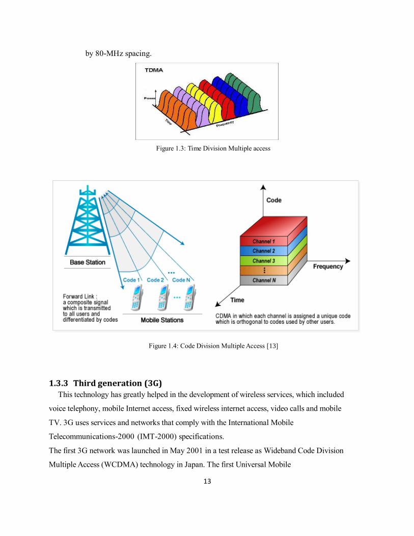
1.4 Global mobile subscribers and market share by technology:
Manystudieshaveshownthegrowingglobaldemandforthethirdandfourthgeneration
systems,thoughthesecondgenerationsystemsstilloccupiestheleadgloballyintermsofuse.
Accordingtothe“4gamericas”website,thepercentageofnetworksthatusetheGSMtechnology
in2015 is54%while theuseofHSPA network reached27.6% andLTE systems is10.45%
[17],asshowninFigure1.5.
Figure 1.5:Globalmobilesubscribersandmarketsharebytechnology
1.5 Frequency bands of generations:
1.5.1 Frequencies of GSM 900-1800 bands GSM-900 and GSM-1800 are used in most parts of the world: Europe, Middle
East, Africa, Australia, Oceania (andmostof Asia)asshowninFigure1.6.
GSM-900 uses 890–915 MHz to send information from the mobile station to the base
station (uplink)and935–960 MHzfortheotherdirection(downlink),providing124RFchannels
(channelnumbers1to124)spacedat200 kHz.Duplexspacingof45 MHzisused.Guardbands
100 kHzwideareplacedateitherendoftherangeoffrequencies.[18]
GSM-1800 uses 1,710 –1,785 MHz to send information from the mobile station to the base
transceiverstation(uplink)and1,805–1,880 MHzfortheotherdirection (downlink),providing

18
374 channels (channel numbers 512 to 885). Duplex spacing is 95 MHz. GSM-1800 is also
calledDCS(DigitalCellularService)inthe UnitedKingdom
Figure 1.6:GSM(GroupSpecialMobile)-GlobalSystemforMobilecommunications-mostpopularstandard
forphonesintheworld.GSM900/GSM1800MHzareusedinmostpartsoftheworld:Europe,Asia,
Australia,MiddleEast,andAfrica.GSM850/GSM1900MHzareusedintheUnitedStates,Canada,Mexico
andmostcountriesofS.America. [19]
1.5.2 Frequencies of 3G bands ThemainUMTS/WCDMAfrequencybandsforFDDoperationaresummarizedintable1.3.
Table 1.3:3GUMTSFREQUENCYBANDS–FDD[20]
3GUMTSFREQUENCYBANDS–FDD
BAND
NUMBER
BAND COMMON
NAME
UL
FREQUENCIES
DL
FREQUENCUES
1 2100 IMT 1920-1980 2120-2170
2 1900 PCSA-F 1850-1910 1930-1990
3 1800 DCS 1710-1785 1805-1880
4 1700 AWSA-F 1710-1755 2110-2155
5 850 CLR 824-849 869-894

19
6 800 830-840 875-885
7 2600 IMT-E 2500-2570 2620-2690
8 900 E-GSM 880-915 925-960
9 1700 1749.9-1784.9 1844.9-1879.9
10 1700 EAWSA-G 1710-1770 2110-2170
11 1500 LPDC 1427.9-1447.9 1475.9-1495.9
12 700 LSMH 699-716 729-746
13 700 USMHC 777-787 746-756
14 700 USMHD 788-798 758-768
19 800 832.4-842.6 877.4-887.6
20 800 EUDD 832-862 791-821
21 1500 UPDC 1447.9-1462.9 1495-1510.9
22 3500 3410-3490 3510-3590
25 1900 EPCSA-G 1850-1915 1930-1995
26 850 ECLR 814-849 859-894
Frequencybands15,16,17,18,23and24arenowreservedfrequencybands.
1.5.3 Frequencies of 4G Bands:
TheLTEnetworksusetwotypesoftechnology,FDD,TDD.TheFDDuse2frequenciesone
foruplink,otherfordownlinkandbetweenthem thereisagapasshowninFigure1.7.Thegap
mustbe sufficienttoenable theroll-offoftheantenna filtering togive sufficientattenuationof
thetransmittedsignalwithinthereceiveband.[21]
Figure 1.7:frequenciesseparatedbygap

20
TheTDDusesthesamefrequencyandbeingtimemultiplexed.
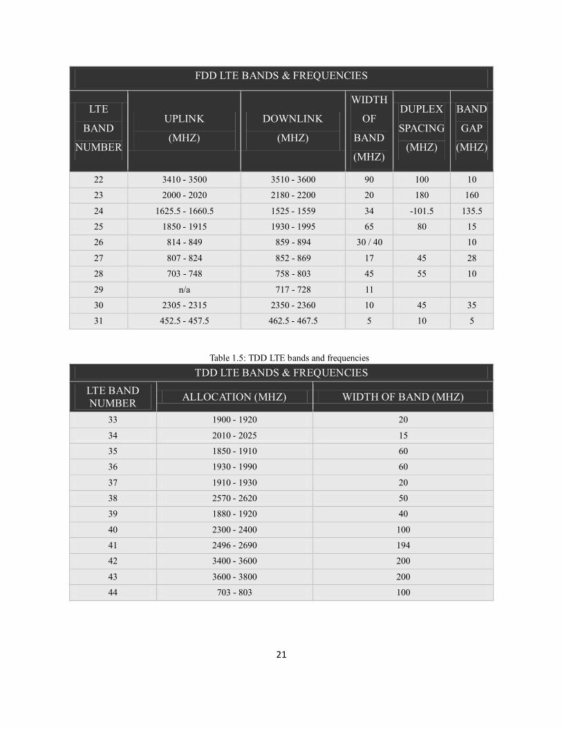
TheLTE frequency band has been divided formany sub bands, and eachbandhasa number.
Currently the LTE bands between 1 & 22 are for paired spectrum, i.e. FDD, andLTE bands
between 33 & 41 are for unpaired spectrum, i.e. TDD. [21]. Table 1.4 shows the FDD LTE
bands,whileTable1.5showstheTDDLTEbands.
Table 1.4:FDDLTEbandsandfrequencies
FDDLTEBANDS&FREQUENCIES
LTE
BAND
NUMBER
UPLINK
(MHZ)
DOWNLINK
(MHZ)
WIDTH
OF
BAND
(MHZ)
DUPLEX
SPACING
(MHZ)
BAND
GAP
(MHZ)
1 1920-1980 2110-2170 60 190 130
2 1850-1910 1930-1990 60 80 20
3 1710-1785 1805-1880 75 95 20
4 1710-1755 2110-2155 45 400 355
5 824-849 869-894 25 45 20
6 830-840 875-885 10 35 25
7 2500-2570 2620-2690 70 120 50
8 880-915 925-960 35 45 10
9 1749.9-1784.9 1844.9-1879.9 35 95 60
10 1710-1770 2110-2170 60 400 340
11 1427.9-1452.9 1475.9-1500.9 20 48 28
12 698-716 728-746 18 30 12
13 777-787 746-756 10 -31 41
14 788-798 758-768 10 -30 40
15 1900-1920 2600-2620 20 700 680
16 2010-2025 2585-2600 15 575 560
17 704-716 734-746 12 30 18
18 815-830 860-875 15 45 30
19 830-845 875-890 15 45 30
20 832-862 791-821 30 -41 71
21 1447.9-1462.9 1495.5-1510.9 15 48 33
21
FDDLTEBANDS&FREQUENCIES
LTE
BAND
NUMBER
UPLINK
(MHZ)
DOWNLINK
(MHZ)
WIDTH
OF
BAND
(MHZ)
DUPLEX
SPACING
(MHZ)
BAND
GAP
(MHZ)
22 3410-3500 3510-3600 90 100 10
23 2000-2020 2180-2200 20 180 160
24 1625.5-1660.5 1525-1559 34 -101.5 135.5
25 1850-1915 1930-1995 65 80 15
26 814-849 859-894 30/40 10
27 807-824 852-869 17 45 28
28 703-748 758-803 45 55 10
29 n/a 717-728 11
30 2305-2315 2350-2360 10 45 35
31 452.5-457.5 462.5-467.5 5 10 5
Table 1.5:TDDLTEbandsandfrequencies
TDDLTEBANDS&FREQUENCIES
LTEBAND
NUMBER ALLOCATION(MHZ) WIDTHOFBAND(MHZ)
33 1900-1920 20
34 2010-2025 15
35 1850-1910 60
36 1930-1990 60
37 1910-1930 20
38 2570-2620 50
39 1880-1920 40
40 2300-2400 100
41 2496-2690 194
42 3400-3600 200
43 3600-3800 200
44 703-803 100
22
1.6 Thesis objective
Nowadaysweneedtopreventsomesignalsenteringsomeareas.Forexampleinintensivecare
rooms in hospitals we must prevent mobile calls without using jammers, and so places of
worship,prisons,securedmeetingrooms,andotherplaces.
Inthisresearchweintendtodesignafrequencyselectivesurface(FSS)toachievethisgoal.The
circuitwillbedesignedusingmicrostriptechnologyonprintedcircuitboardthatcanbemounted
onawallandwirenetthatcanbebuiltinopenareas.Thesignalsofinterestheretobeblockedis
thedownlinkbandsofmulticellularnetworksthatareusedinHistoricalPalestine.[22],[23]
Bandsthatwillbecoveredthroughtheresearchare:
GSMsignal(925-960MHz),(1805-1880MHz).
3Gmobilenetwork(2110-2170MHz).
Band7ofLTEsystems(2620–2690MHz).
1.7 Thesis overview:
Thethesisconsistsoffourchapters
The first chapter briefly reviewed the differentgenerations ofmobile phone networksand the
most important characteristics and also the global ranges for each generation.Also the most
importantapplicationsoftheFSStechniquearepresented.
Inthe secondchapterthetheoreticalbackgroundofthe frequencyselective surfaces(FSS)and
themostimportantdesignsusedwillbepresented.Moreover,mathematicalequationsforsome
knownFSSstructuresarepresented.
In the third chapter some researches and designs published in literature on the subject of the
thesiswillbeintroduced,andalsofourFSSdesignsalongwiththeirwillbepresented.
Chapterfourshowstheconclusionsdrawnfromthecurrentworkinadditiontofuturework.

23
Chapter 2: Frequency Selective Surface Theory
Frequency Selective Surfaces are a periodic structures etched in a dielectric surface or a
group of metallic structures in vacuum. These shapes are resonant with some frequencies
dependingonlengthsandtypeofmaterials,andtheselectivesurfacesworkasbandpassorband
stop filters depending on type ofmetallic elementspatch oraperture.Thepatch elementarray
behavesasabandstopfilterandtheapertureelementarrayactsasabandpassfilterasshownin
Figure2.1[24].
Figure 2.1:(a)patchelements,(b)apertureelements
Many factorsare involved inunderstanding the operationandapplicationof frequency
selective surfaces. These include analysis techniques, operating principles, design principles,
manufacturing techniques and methods for integrating these structures into space, ground and
airborneplatforms.Theoverall frequencyresponseincludingitsbandwidthanddependenceon
the incidence angle and polarization is determined by the element geometry and the substrate
parameters.[25]
2.1 The relevant concepts in electromagnetic theory
To understand the underlying mechanism on which the filters function. As shown in
Figure 2.2, an incident plane wave strikes the filter and causes the electrons in the metal to
oscillate. Ifalargeportionofthe incidentenergyisabsorbedbytheseelectrons theyre-radiate
andcanceltheinitialfield,causingthetransmittancethroughthefiltertobelow.Inthiscase,the

24
electronswill re-radiate toward the left and cause the reflectedwaveamplitude to be high. If
only a small portion of the incident power is absorbed no such cancellation occurs and the
transmittance will be high. In general the transmittance through the filter is a function of
frequency;inotherwords,theelectronsinthemetalwillabsorbandre-radiatesomewavelengths
withhigherefficiencythanothers.Theshapeofthetransmittancecurvedependsonthepattern
etchedintothemetal filter,andwecanetchvariouspatternsintoourmetaltoobtain filtersof
varyingbehavior.[26]
Figure 2.2:(a)Electroninfilterplaneundergoesoscillationsdrivenbysourcewave,(b)Electronconstrainedto
movealongwirecannotundergooscillations.
2.2 Filter Geometries and Equivalent Circuits:
Althoughthesimulationsoftwareanalyzesthegeometrieswedesignaccurately,weoftenneedto
understand the physical background behind the geometries in which we design. The most
common shapes used in FSS and their equivalent circuits and mathematical analysis are
presentedhere.
The three most common types of filters are: strip grating filters, mesh filters, and cross-mesh
filters.The first typeisused toillustratethetheoreticalideaof filter,the secondtypeisuseful
becauseoftheirpolarization-independenceproperty,andthethirdtypethatweareinterestedin
isusedasband-passandband-stopfilters.

25
2.3 Strip Grating Filters:
ThegeometryofthestripgratingfilterisshowninFigure2.3[26].IftheE-fieldisparalleltothe
metalstripswehaveaninductivestrip-gratingfilterasshowninFigure2.4(left);iftheE-fieldis
perpendiculartothestripswehaveacapacitivestrip-gratingfilterasshowninFigure2.4(right).
Figure 2.3:IftheE-fieldisperpendiculartothestripsthefilterswitchesbetweenstatesaandb,ifitisparallel
tothestripthefilterswitchesbetweencandd.
Figure 2.4:strip-gratingfiltersanditsequivalentcircuit

26
Modelingarraysatobliqueanglesofincidencethereforerequiresexpressionsfortheadmittances
forbothtransverse electric (TE)andtransverse magnetic(TM)incidence.
TM-incidenceoccurswhentheE-fieldispolarizedparalleltotheplaneofincidence,i.e.θ=0°,
andTE-incidencewhen theE-fieldisperpendicular totheplaneof incidence,i.e.Φ=0°[27].
UsingthegeometryofFigure2.5,forconductorsofperiodicityp,widthw,andspacedadistance
g,Marcuvitzgavenormalizedadmittanceexpressionsfortwocases[28]:
Figure 2.5:Planewaveincidentonaninductivestripgrating,foracapacitivestripgratingexchangetheincident
electricfieldEforamagneticfieldH
Thenormalizedshuntinductivereactanceexpressionoftheinductivestripgratingwasgivenby
Marcuvitzas:
𝑋𝑇𝐸 = 𝑤.
𝐿
𝑍𝑂= 𝑝.
cos𝜃
𝜆. (ln (𝑐𝑜 𝑒𝑐 (
𝜋𝑤
2𝑝)) + 𝐺(𝑝, 𝑤, 𝜆, 𝜃)) (2.1)
ThenormalizedshuntsusceptanceexpressionofthecapacitivestripgratingwasgivenbyLeeas:

27
𝐵𝑇𝐸 = 𝑤.
𝐶
𝑌𝑂= 4𝑝.
𝑒𝑐 𝜃
𝜆. (𝑙𝑛 (𝑐𝑜 𝑒𝑐 (
𝜋𝑔
2𝑝)) + 𝐺(𝑝,𝑤, 𝜆, 𝜃)) (2.2)
WhereGisthecorrectiontermgivenas:
𝐺(𝑝,𝑤, 𝜆, 𝜃) = .5(1 − 𝛽 ) [(1 −
𝛽
4) (𝐴 + + 𝐴 −) + 4𝛽
𝐴 +𝐴 −]
(1 −𝛽
4) + 𝛽 (1 +
𝛽
2−𝛽4
8)(𝐴 + + 𝐴 −) + 2𝛽
6𝐴 +𝐴 −
(2.3)
𝐴 ± =
1
√(𝑝 𝑖𝑛 𝜃𝜆
± 1) − 𝑝 /𝜆 − 1
(2.4)
𝛽 = 𝑖𝑛(
.5𝜋𝑤
𝑝) (2.5)
Theseequationsarevalidforwavelengthandanglesofincidentθintherange ( + )/
2.4 Mesh Filters:
As shown in Figure 2.6, the capacitive mesh consists of a grid of metal squares while the
inductivemeshrepresentsthecomplementarystructure.Thesefilterswillalsobehaveaslow-and
high-pass filters but have the additional advantage that the transmittance through the filter is
independentofthepolarizationofthesource[26].
28
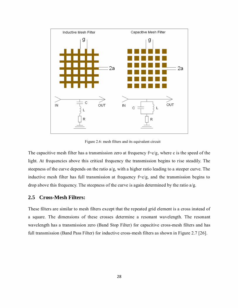
Figure 2.6:meshfiltersanditsequivalentcircuit
Thecapacitivemeshfilterhasatransmissionzeroatfrequencyf=c/g,wherecisthespeedofthe
light.At frequenciesabove this critical frequency the transmission begins to rise steadily.The
steepnessofthecurvedependsontheratioa/g,withahigherratioleadingtoasteepercurve.The
inductive mesh filter has full transmission at frequency f=c/g, and the transmission begins to
dropabovethisfrequency.Thesteepnessofthecurveisagaindeterminedbytheratioa/g.
2.5 Cross-Mesh Filters:
Thesefiltersaresimilartomeshfiltersexceptthattherepeatedgridelementisacrossinsteadof
a square. The dimensions of these crosses determine a resonant wavelength. The resonant
wavelengthhasatransmissionzero(BandStopFilter)forcapacitivecross-mesh filtersandhas
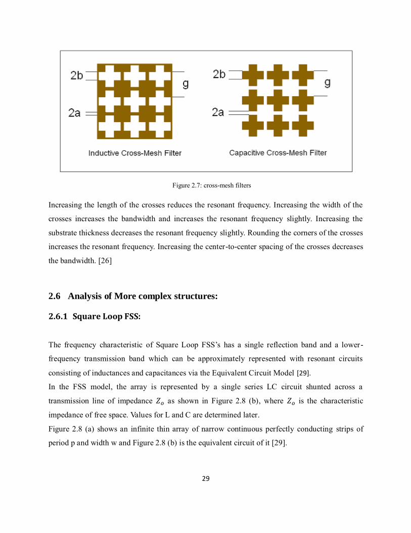
fulltransmission(BandPassFilter)forinductivecross-meshfiltersasshowninFigure2.7[26].
29
Figure 2.7:cross-meshfilters
Increasingthe lengthof thecrossesreducestheresonant frequency.Increasingthewidthofthe
crosses increases the bandwidth and increases the resonant frequency slightly. Increasing the
substratethicknessdecreasestheresonantfrequencyslightly.Roundingthecornersofthecrosses
increasestheresonantfrequency.Increasingthecenter-to-centerspacingofthecrossesdecreases
thebandwidth.[26]
2.6 Analysis of More complex structures:
2.6.1 Square Loop FSS:
The frequency characteristic of Square Loop FSS’s has a single reflection band and a lower-
frequency transmission band which can be approximately represented with resonant circuits
consistingofinductancesandcapacitancesviatheEquivalentCircuitModel[29].
In the FSS model, the array is represented by a single series LC circuit shunted across a
transmission line of impedance 𝑍𝑜 as shown in Figure 2.8 (b), where 𝑍𝑜 is the characteristic
impedanceoffreespace.ValuesforLandCaredeterminedlater.
Figure2.8 (a) showsan infinite thinarray ofnarrow continuous perfectlyconducting strips of
periodpandwidthwandFigure2.8(b)istheequivalentcircuitofit[29].

30
Figure 2.8:a)Layoutofsquarelooparrays,b)Equivalentcircuit
Figure 2.9:analysisofsquareloopFSS
ThenormalizedshuntinductivereactanceexpressionofthesquareloopFSSis[29]
𝑋𝑇𝐸 = 𝐹(𝑝, 2𝑤, 𝜆) (2.6)
𝑋𝑇𝐸 = 𝑤.
𝐿
𝑍𝑂= 𝑝.
𝑐𝑜 𝜃
𝜆. (𝑙𝑛 (𝑐𝑜 𝑒𝑐 (
2𝜋𝑤
2𝑝)) + 𝐺(𝑝, 𝑤, 𝜆, 𝜃)) (2.7)
Gisobtainedfromeq.2.3

31
𝑋𝑇𝑀 = 𝑝.
𝑒𝑐 ∅
𝜆. (𝑙𝑛 (𝑐𝑜 𝑒𝑐 (
2𝜋𝑤
2𝑝)) + 𝐺(𝑝, 𝑤, 𝜆, ∅)) (2.8)
Thenormalizedshuntsusceptanceexpressionofthecapacitivestripgrating
𝐵𝑇𝑀 = 4𝐹(𝑝, 𝑔, 𝜆) = 4𝑝.
𝑐𝑜 ∅
𝜆. (𝑙𝑛 (𝑐𝑜 𝑒𝑐 (
𝜋𝑔
2𝑝)) + 𝐺(𝑝, 𝑔, 𝜆, ∅)) (2.9)
𝐵𝑇𝐸 = 𝑤.
𝐶
𝑌𝑂= 4𝑝.
𝑒𝑐 𝜃
𝜆. (𝑙𝑛 (𝑐𝑜 𝑒𝑐 (
𝜋𝑔
2𝑝)) + 𝐺(𝑝,𝑤, 𝜆, 𝜃)) (2.10)
ThesurfaceimpedanceofFSSis
𝒁 = 𝒋𝒘𝑳 +
𝒋𝒘𝑪= 𝒋(𝒘𝑳 −
𝒘𝑪) (2.11)
Thereflectioncoefficientis[30]
𝑆 = −
1
2𝑍𝑍𝑜+ 1
(2.12)
For square loop FSS etched into dielectric substrate, the equivalent circuit is shown inFigure
2.10[31].
Figure 2.10:equivalentcircuitforsquareloop
The Inductive reactance element is calculated as in eq.2.13

32
𝑋𝑓
𝑍𝑜=
1
√𝜀𝑒.𝑑
𝑝. 𝐹(𝑝, 2𝑤, 𝜆𝑒) (2.13)
F is obtained from eq.2.6
And the capacitance reactance element is calculated as in eq.2.14
𝐵𝑓. 𝑍𝑜 =
4𝑑
𝑝.√𝜀𝑒𝐹(𝑝, 𝑔, 𝜆𝑒) (2.14)
Theeffectivewavelength
𝜆𝑒 = 𝜆/(𝜺𝒆)−𝟎.𝟓 (2.15)
Theeffectivepermittivityisgivenby
𝜀𝑒 =
𝜀𝑟 + 1
2+𝜀𝑟 − 1
2.
1
√1 +12𝑡𝑤
(2.16)
Wheretisthethicknessofsubstrateandεristhepermittivityofdielectric
Itcanbeseenthattheimpedance𝑋𝑓/𝑍𝑜isreducedbyafactor d/p.Athindielectricsubstrate,on
whichtheconductiveelementsareprinted,causesanincreaseinthesusceptance(𝐵𝑓. 𝑍𝑜)ofthe
arraywhilenoeffectontheinductivereactanceisobserved.[32]
2.6.2 Jerusalem Cross:
Jerusalem Cross is one of the other well-known forms, where there are a number of
computationalanalysistocalculatethefrequencyandbandwidthtobeachieved.
Assuming a vertically polarized wave is normally incident on the grid, Leonard and Cofer
developedanequivalentcircuitmodelfortheJerusalemcross,consistingofacombinationof
twoLCresonantcircuitsinseries,asillustratedinFigure2.11,2.12[33]

33
Figure 2.11:Jerusalemcrossperiodicarray
Figure 2.12:equivalentcircuitofJerusalemcross
Figure 2.13 shows the frequency response of Jerusalem cross FSS
Figure 2.13:frequencyresponseofJerusalemcross
Thevalueofeachinductivestrip𝑋𝐿ofwidthwiscalculatedusing
𝑋𝐿
𝑍𝑂= 𝐹(𝑝, 𝑤, 𝜆, ∅) = 𝑝.
𝑐𝑜 ∅
𝜆. (𝑙𝑛 (𝑐𝑜 𝑒𝑐 (
𝜋𝑤
2𝑝)) + 𝐺(𝑝,𝑤, 𝜆, ∅)) (2.17)
34
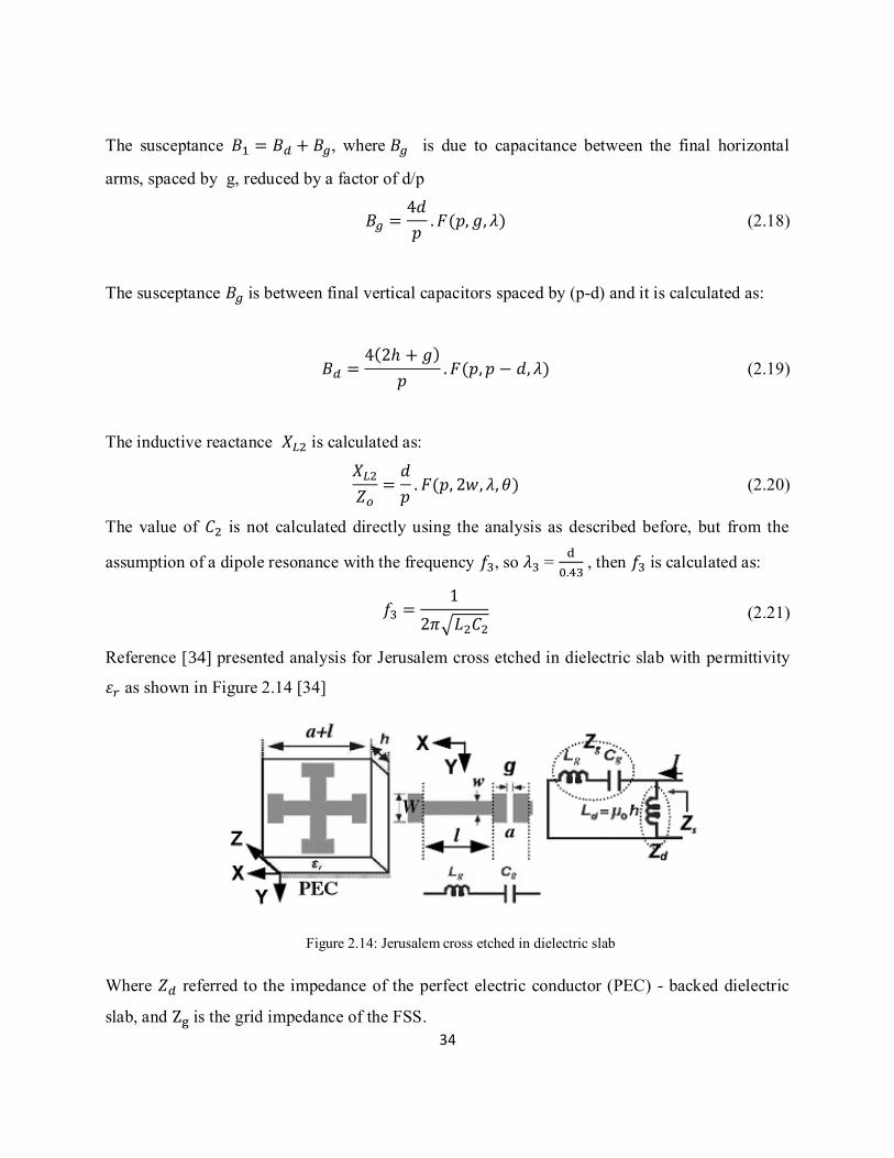
The susceptance 𝐵 = 𝐵𝑑 + 𝐵𝑔, where 𝐵𝑔 is due to capacitance between the final horizontal
arms,spacedbyg,reducedbyafactorofd/p
𝐵𝑔 =
4𝑑
𝑝. 𝐹(𝑝, 𝑔, 𝜆) (2.18)
Thesusceptance𝐵𝑔isbetweenfinalverticalcapacitorsspacedby(p-d)anditiscalculatedas:
𝐵𝑑 =
4(2 + 𝑔)
𝑝. 𝐹(𝑝, 𝑝 − 𝑑, 𝜆) (2.19)
Theinductivereactance𝑋𝐿 iscalculatedas:
𝑋𝐿
𝑍𝑜=𝑑
𝑝. 𝐹(𝑝, 2𝑤, 𝜆, 𝜃) (2.20)
The value of𝐶 is not calculated directlyusing theanalysis asdescribedbefore, but from the
assumptionofadipoleresonancewiththefrequency𝑓3,so𝜆3=d
.43,then𝑓3iscalculatedas:
𝑓3 =
1
2𝜋√𝐿 𝐶 (2.21)
Reference[34]presentedanalysisforJerusalemcrossetchedindielectricslabwithpermittivity
𝜀𝑟asshowninFigure2.14[34]
Figure 2.14:Jerusalemcrossetchedindielectricslab
Where𝑍𝑑referredtotheimpedanceoftheperfect electricconductor(PEC) -backeddielectric
slab,andZgisthegridimpedanceoftheFSS.

35
2.7 A brief of most common FSS geometries
Table 2.1 illustrates a brief of most common FSS geometries [35].
Table 2.1:abriefofmostcommonFSSgeometriesanditsequivalentcircuits

36
2.8 Literature review
In [36], asquareloopFSSstructure(7×7)isdesigned and simulatedat2.4GHz.Thetwo
materialsofdielectricsubstratewhichareFR4boardandglasshavebeenusedtoproducehybrid
materials.Sixtypesofhybridconfigurationshavebeenstudied.Theresultsshowthatthereturn
loss and transmission signal are effected by using hybrid materials which led to the compact
structure.Thedisadvantageofthisdesignthatitcoversonlyoneband.
In [37], FSSs are deployed to selectively confine radio propagation in indoor areas, by
artificially increasing the radio transmission loss naturally caused by building walls. FSS can
alsobeusedtochannelradiosignalsintootherareasofinterest.Simulationsandmeasurements
have been carried out in order to verify the frequency selectivity of the FSS. Practical
considerations regarding the deploymentofFSS onbuildingwalls and the separation distance
betweentheFSSandthesupportingwallhavebeenalsoinvestigated.Acontrolled,small-scale
indoor environment has been constructed and measured in an anechoic chamber in order to
practicallyverifythisapproachthroughtheusageofraytracingtechniques.
TheresultssuggestthatproperFSSdeploymentcanbeusedinindoorwirelessenvironmentsin
ordertoincreaseorrestrict coverageand thatRayTracingtechniquescanbeapplied topredict
radiopropagationinsuchenvironments.ProperFSSdeploymentcanassistsignalchannelingor
confinecoverageinspecificareas.Thedisadvantageofthisdesignthatthecellsizeislargeand
itcoversonlyoneband.
In [38], FrequencySelectiveSurface(FSS)isusedasasubreflectorinasatellite.TheFSS
is designed by cutting slots in the square patch keeping same periodicity throughout.
Frequency-selectivesurfacesarespatialfilterswhichwhenincorporatedaseitherflatorcurved
sub reflectors into a reflector antenna allows it to operate at a number of different frequency
bands. This designed FSS structure has a wide stop band from 3.70GHz to 6.23GHz with
percentagebandwidthof51.Sizereductionupto83%isalsoachieved.
In [39], Asimpleandfastapproachtodesignathinandwidebandradarabsorbingstructure
ispresented.Theproposedmethodisapplicablefordesignofanabsorberconsistingof
anynumberoflayersandanytypesofFSS,togetherwithanygivenmaterialthatwillbe
usedforlayerseparation.AnexampleofRadarAbsorbingMaterial(RAM)designedby
using the proposedmethodology is also presented. The given RAM is a two layered
structurebackedbyagroundplane.ThelayersareconsistingofresistiveFSSpatterns,
namely square ring and crossed dipole. Simulation results carried out by the high
frequencystructural simulator(HFSS)tool showedthattheproposedapproach is agood

37
candidatefordesigningthinandwidebandradarabsorbingstructures.Butthisdesignisunstable
atobliqueincidences.
In [40], Aseriesofnovelminiaturizedfrequencyselectivesurfacesconsistofcombinations
ofrectanglespiral-basedelementsareproposed.Thesimulationresultsshowthatusingrectangle
spiral-based structures instead of the meander line FSS provides at least 56% reduction of
resonant frequencies.Moreover, the novelFSSs have excellent angle stabilityand polarization
stability.Accordingly,thenovelminiaturizedFSSshavegreatpotentialforpracticalapplications
inlimitedspace.Butthetransmissioncoefficientreducedabout20dB.
In [41], Ithasbeen shown that a bandpass FSS can be designed simply byusing lumped
reactivecomponents.Thefulldesignmethodologyhasbeenpresented,resultinginthepotential
to design FSS with unit cell sizes. It has been shown that the resonant frequency can be
controlled with the choice of lumped component values and to some extent the path length
between the components. For practical designs the values of componentswill be available in
discrete steps,however, finetuningoftheresonant frequencycanbeachievedbychangingthe
pathlength.Theeffectoftheresistanceassociatedwiththecomponentshasbeenevaluatedand
canbeminimizedbymaximizingL/Candthepathlengthbetweenthecomponents.Theoblique
incidenceperformanceoftheFSSis stable forbothpolarizationsandmethods formaintaining
transmissionlossatanacceptablelevelhavebeenpresented.Thistechnologycanbeappliedto
low frequency radome and antenna applications, where physical volume is limited. The
disadvantageofthisdesignthatitcoversonlyoneband.
In [42], Frequency selective shielding of aroomat themost used communication
bands of GSM 900 MHz, 1800MHz and 2400MHz is designed using Jerusalem cross
elements.Minimumof20dBof shieldingisachievedat theabovebands. Thedesignedtri -
band band-stop filter has stable frequency response for varying incidenceangles and
polarization, which is the important requirement. The factors influencing the resonance
frequencyandbandwidtharealsodiscussed.Butthedesignedmodelmaybenotpracticalwith
3GandLTEnetworks.
In [43], Theshieldingeffectivenessoffrequencyselectivesurfaces(FSS)withdoublesquare
elementsreflectingat900MHzand1800MHzareanalyzedusingmodalexpansiontechniques.
Ithasbeen shownthatthe shieldingeffectivenessof the structure isgreater than60dBat900
MHzandgreaterthan40dBat1800MHz.Butthedesignedmodelmaybenotpracticalwith3G
andLTEnetworks.
38
Chapter 3: Designs and simulations of Frequency Selective Surfaces
3.1 Introduction
Manydesignsadoptedbasicallyonpopularmodelssuchassquareloop,Jerusalemcrossand
triplepolestoworktheFSS.Theprobleminthesedesignsthelimitedbandsthatcanbecovered
inonedesign.Thisreasonledtotheinnovationofmanynewshapesintwoandthreedimensions
inordertoachievemultibandsandminimizethesizeofthemodel.
3.2 Designs and simulations:
3.2.1 Goals of designs:
The circuit will be designed using microstrip technology on printed circuit board that can be
mountedonawall,andwirenetthatcanbebuiltinopenareas.Thesignalofinterestheretobe
blocked is the downlink bands formulti cellularnetworks that areused inHistoricalPalestine
[18],[19].
FrequencyBandsthatareconsideredinthedesignshereare:
GSMsignal(925-960MHz),(1805-1880MHz).
3Gmobilenetwork(2110-2170MHz).
Band7ofLTEsystems(2620–2690MHz).
3.2.2 Simulation Software CST: Thedesignsand simulationsin thisprojectarebasedontheComputerSimulationTechnology
(CST)MicrowaveStudioSuitewhichisahighperformanceelectromagneticsimulationsoftware
[44].Thereare twobasic solvermodules provided: timedomain solverand frequency domain
solver. The two solvers are totally different. Time domain solver is used for non-resonant
structures and frequency domain solver contains alternatives for highly resonant structures.
Besidesfrequencydomainsolverhastheoptionofutilizingtetrahedralmeshthatcandiscretethe
structurebetterwhichisnotavailablewithintimedomainsolver.Inaddition,timedomainsolver
isonlyfornormalincidencebutfrequencydomainsolvercanbeusedforoff-normalincidences.
BecauseoftheaboveIusedthefrequencydomainsolvertosimulatedesigns.
3.3 Basics of the designs:
Designs are mainly based on the shapes of square loop and Jerusalem cross, some modifications are
added to achieve the desired resonances. After that, some of the designs were not stable with varying
the polarization so the rotation of the shapes four times clockwise occurred to solve this problem.

39
3.4 Bandstop double square loop FSS:
3.4.1 Structure of FSS: TheunitcelldimensionsofbandstopFSSareshowninFigure3.1.Thebandstopcharacteristics
areachievedbydesigningtwosquare-loopelementsofdifferentdimensionsonFR-4substrate.
The thicknessofFR-4substrateis1.6mmaand relativepermittivity(𝜀𝑟)andthelosstangent
(tan δ) are 4.3 and 0.02, respectively. The periodicity of unit cell is 81.5×81.5mm . The
circumferenceoftheoutersquare-loopelementis278mmwhichistunedto900MHzwhile
thecircumferenceoftheinnersquareloopelementis209mmwhichistunedto1800MHz.
The width of both square loop elements is 5.8 mm.The dimensions of the FSS structure are
depictedinTable3.1.
Figure 3.1:a)dimensionsofsquareloopFSS,b)sideviewofthemodel
Table 3.1:dimensionsofthedesign
Name L1 L2 W1 W2 g h εr t
Value (mm) 69.5 52.25 5.8 5.8 12 1.6 4.3 0.1

40
3.4.2 Simulation results:
TheunitcellofFSSwhichisshowninFigure3.2issimulatedbyapplyingperiodic
boundary conditions using CST Microwave Studio, commercially available electromagnetic
software.Thetransmissionandreflectioncoefficientsareobtainedfrom400-4000MHzfor
bothTMandTEpolarizationsatobliqueincidences.
Figure 3.2:a)periodicFSS,b)FSSmodelwithincidentplanewave
InFigure3.3,thetransmissionandreflectioncoefficientsarepresentedforTMpolarizationfor
and45 angleofincidence.Theresonantfrequenciesat are932.8MHzand1825.6MHz,
whileat45 ,theseare947.2MHzand1750MHz,respectively.Thecorrespondingtransmission
coefficients are -28dB, -42dBat , and -25dBand -38dBat45 .The shift in resonant
frequencyfrom to45 isabout14.4MHzatband900MHzandabout-75.6MHzat
band1800MHz.ThisshowsthatFSShasastablefrequencyresponseastheangleof
incidencevaried from to45 .It isdemonstratedthat the shiftinresonantfrequencies is
occurredduetothemutualcouplingbetweentheFSSelements.

41
Figure 3.3:Simulationresultsofdual-bandstopFSSforTMpolarization
InFigure3.4, thetransmissionandreflectioncoefficientsarepresented forTEpolarization for
and45 angleofincidence.Theresonantfrequenciesat are936.4MHzand1825.6MHz,
whileat45 ,theseare947.2MHzand1750MHz,respectively.Thecorrespondingtransmission
coefficients are -28dB, -42dBat , and -25dBand -38dBat45 .The shift in resonant
frequencyfrom to45 isabout10.8MHzatband900MHzandabout-75.6MHzat
band1800MHz.ThisshowsthatFSShasastablefrequencyresponseastheangleof
incidencevariedfrom to45 .Tables3.2and3.3showsimulationresultsforbothTMand
TEpolarizations.
Figure 3.4:Simulationresultsofdual-bandstopFSSforTEpolarization
Table 3.2:-10dBtransmissionbandwidthsat900/1800MHzforTMpolarization
900 MHz 1800 MHz
Angle Resonant frequency fr1 (MHz)
Bandwidth BW (MHz)
Resonant frequency fr2 (MHz)
Bandwidth BW (MHz)
TE 932.8 111 1825.6 588.6
TE 45 947.2 79 1750 457.7

42
Table 3.3:-10dBtransmissionbandwidthsat900/1800MHzforTEpolarization
900 MHz 1800 MHz
Angle Resonant frequency fr1 (MHz)
Bandwidth BW (MHz)
Resonant frequency fr2 (MHz)
Bandwidth BW (MHz)
TM 936.4 116.7 1825.6 574.2
TM 45 947.2 79.1 1750 357.7
3.5 Tri bandstop open loop FSS with FR substrate:
Theseconddesign foranFSSstructure ispresentedinFigure3.5. Itisdesignedtocoverthree
bandsGSM900,GSM1800andLTE.
Figure 3.5:overallviewoftheunitcellmodel
3.5.1 Structure of FSS:
TheunitcelldimensionsofbandstopFSSareshowninFigure3.6.Thebandstopcharacteristics
are achieved by designing several elements of different dimensions on FR-4 substrate. The
periodicityofunit cellis63.5×63.5mm .The circumferenceoftheouter squareopen loop
elementis103.9mmwhichistunedto900MHzwhiletheremaininginnerstructureistuned
to 1800 MHz and LTE bands . The width of microstrip is 1.9 mm. Table 3.4 shows the
dimensionsofthestructureinFigure3.6.
43
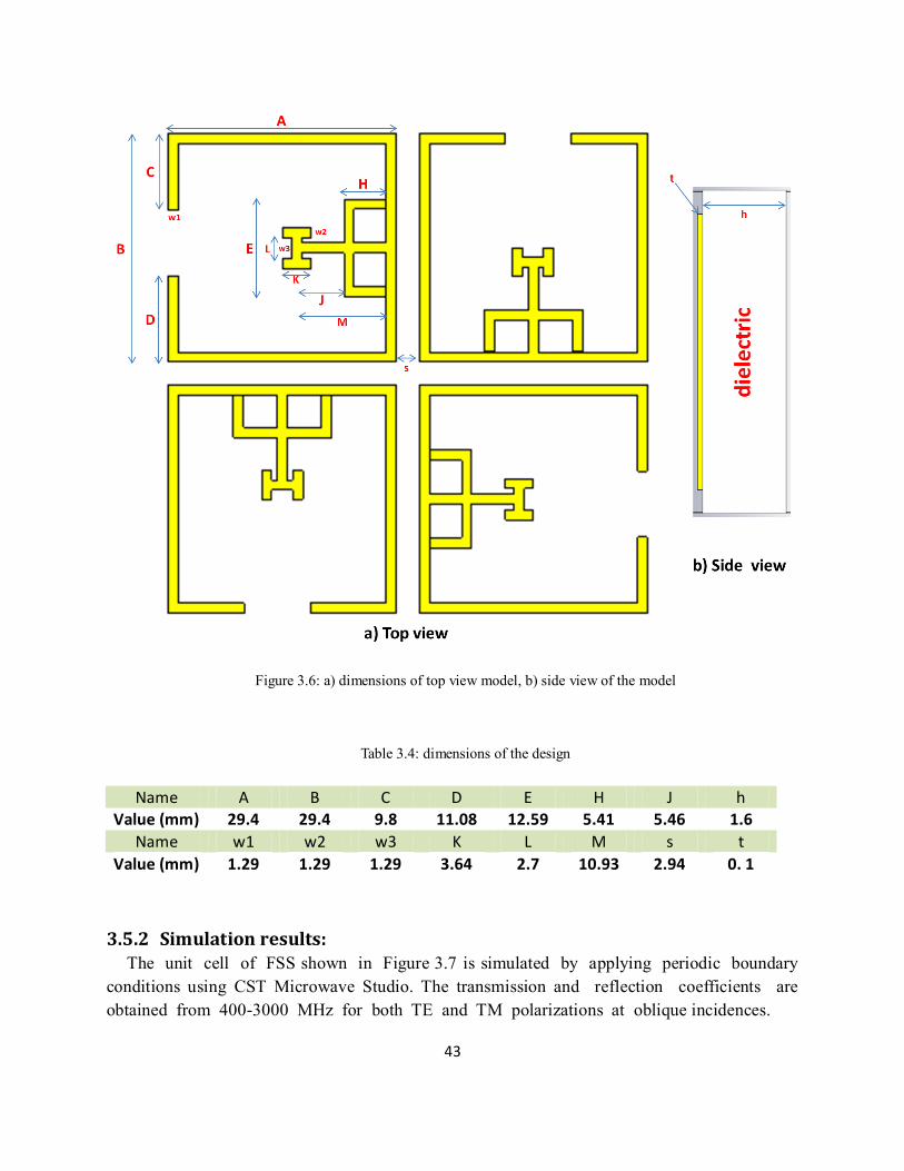
Figure 3.6:a)dimensionsoftopviewmodel,b)sideviewofthemodel
Table 3.4:dimensionsofthedesign
Name A B C D E H J h Value (mm) 29.4 29.4 9.8 11.08 12.59 5.41 5.46 1.6
Name w1 w2 w3 K L M s t
Value (mm) 1.29 1.29 1.29 3.64 2.7 10.93 2.94 0. 1
3.5.2 Simulation results: TheunitcellofFSSshowninFigure3.7issimulatedbyapplyingperiodicboundary
conditions using CST Microwave Studio. The transmission and reflection coefficients are
obtainedfrom400-3000MHzforbothTEandTMpolarizationsatobliqueincidences.
44
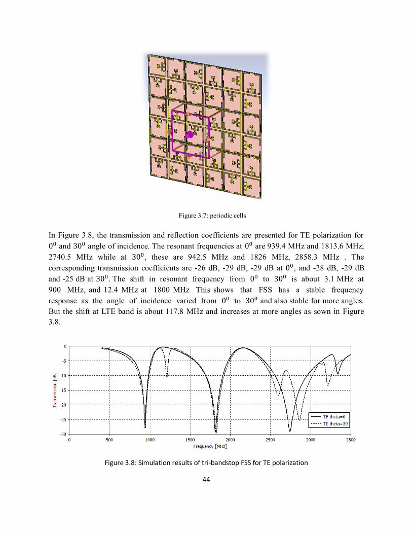
Figure 3.7:periodiccells
InFigure3.8, thetransmissionandreflectioncoefficientsarepresented forTEpolarization for
and3 angleofincidence.Theresonantfrequenciesat are939.4MHzand1813.6MHz,
2740.5 MHz while at 3 , these are 942.5 MHz and 1826 MHz, 2858.3 MHz . The
corresponding transmission coefficients are -26dB, -29dB, -29dBat , and -28dB, -29dB
and-25dBat3 .Theshiftinresonantfrequencyfrom to3 isabout3.1MHzat
900 MHz, and 12.4MHz at 1800MHz This shows that FSS has a stable frequency
responseastheangleofincidencevariedfrom to3 andalsostableformoreangles.
Butthe shiftatLTEbandisabout117.8MHzand increasesatmoreanglesas sown inFigure
3.8.
Figure 3.8: Simulation results of tri-bandstop FSS for TE polarization

45
InFigure3.9,thetransmissionandreflectioncoefficientsarepresentedforTMpolarizationfor
and3 angleofincidence.Theresonantfrequenciesat are939.4MHz,1819.8MHzand
2740.5MHz,whileat3 , theseare939.4MHz,1810.5MHzand2842.8MHz, respectively.
Thecorrespondingtransmission coefficientsare -26dB,-29dB,-29dBat ,and -25dB,-28
dBand-22dBat3 .Theshift inresonantfrequencyfrom to3 isaboutzeroat
900 MHz. and -9.3MHz at 1800MHz This shows that FSS has a stable frequency
responseastheangleofincidencevaried from to3 .But the shift atLTEband is
about102.3MHzandincreasesatmoreanglesassownin Figure3.9.Therefore,itcanbeseen
that the FSS response is sufficiently stable for bothTE andTM polarizations as the angle of
incidence isvaried.Tables3.5and3.6 andFigures3.10,3.11,3.12and3.13 show simulation
resultsforbothTMandTEpolarizations.
Figure 3.9:Simulationresultsoftri-bandstopFSSforTMpolarization
Table 3.5:-10dBtransmissionbandwidthsat900/1800MHzandLTEBandforTEpolarization
900 MHz 1800 MHz LTE Band
Angle Resonant frequency fr1 (MHz)
Bandwidth BW (MHz)
Resonant frequency fr2 (MHz)
Bandwidth BW (MHz)
Resonant frequency fr2 (MHz)
Bandwidth BW (MHz)
TE 939.4 98.8 1813.6 209.6 2740.5 390.2
TE 3 942.5 119.57 1826 220.6 2858.3 502.8
46
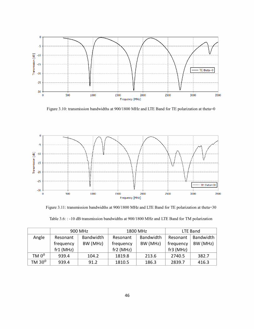
Figure 3.10:transmissionbandwidthsat900/1800MHzandLTEBandforTEpolarizationattheta=0
Figure 3.11:transmissionbandwidthsat900/1800MHzandLTEBandforTEpolarizationattheta=30
Table 3.6::-10dBtransmissionbandwidthsat900/1800MHzandLTEBandforTMpolarization
900 MHz 1800 MHz LTE Band
Angle Resonant frequency fr1 (MHz)
Bandwidth BW (MHz)
Resonant frequency fr2 (MHz)
Bandwidth BW (MHz)
Resonant frequency fr3 (MHz)
Bandwidth BW (MHz)
TM 939.4 104.2 1819.8 213.6 2740.5 382.7
TM 3 939.4 91.2 1810.5 186.3 2839.7 416.3

47
Figure 3.12:transmissionbandwidthsat900/1800MHzandLTEBandforTMpolarizationattheta=0
Figure 3.13:transmissionbandwidthsat900/1800MHzandLTEBandforTMpolarizationattheta=30
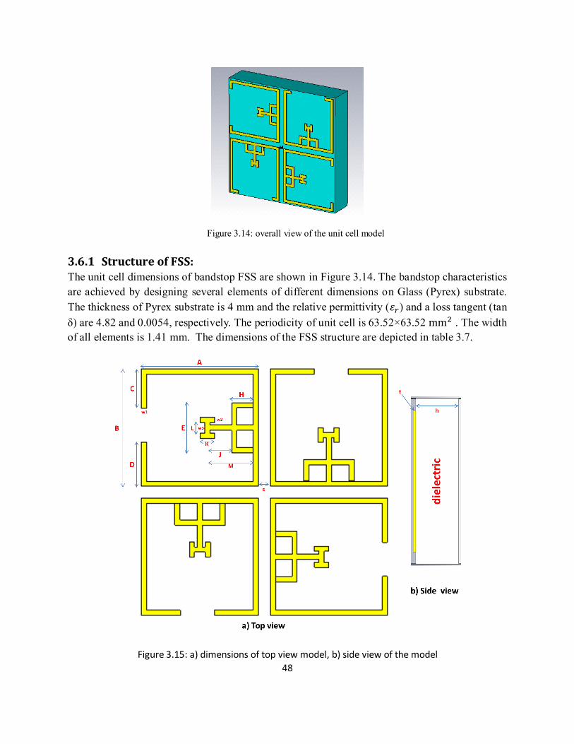
3.6 Tri bandstop open loop FSS with glass (pyrex) substrate:
Mostofbuildingshavewallsofglassthatallowstheunwanted signals topassthrough it.This
requirestodesignmodelsonglasssubstratetogivethebestresultsisolation.Figure3.14shows
thethirddesignforanFSSstructurewhichetchedinglass(pyrex)substrateanditisdesignedto
coverthreebandsGSM900,GSM1800andLTE.
48
Figure 3.14:overallviewoftheunitcellmodel
3.6.1 Structure of FSS: TheunitcelldimensionsofbandstopFSSareshowninFigure3.14.Thebandstopcharacteristics
areachievedbydesigning severalelementsofdifferentdimensionsonGlass(Pyrex)substrate.
ThethicknessofPyrexsubstrateis4mmandtherelativepermittivity(𝜀𝑟)andalosstangent(tan
δ)are4.82and0.0054,respectively.Theperiodicityofunitcellis63.52×63.52mm .Thewidth
ofallelementsis1.41mm.ThedimensionsoftheFSSstructurearedepictedintable3.7.
Figure 3.15: a) dimensions of top view model, b) side view of the model

49
Table 3.7:dimensionsofthedesign
Name A B C D E H J h
Value (mm) 29.4 29.4 4.9 4.22 11.36 4.64 4.7 4
Name w1 w2 w3 K L M s t Value (mm) 1.41 1.41 1.41 3.77 1.76 9.41 2.76 0.1
3.6.2 Simulation results:
Thetransmissionandreflectioncoefficientsareobtainedfrom400-3500MHzforbothTE
andTMpolarizationsatobliqueincidences.
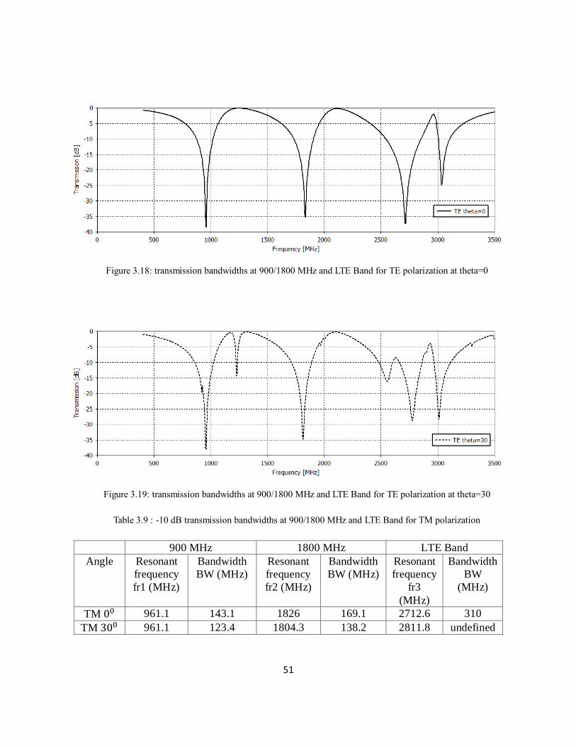
InFigure3.16,thetransmissionandreflectioncoefficientsarepresentedforTEpolarizationfor
and3 angleofincidence.Theresonant frequenciesat are958MHzand1832.2MHz,
2712.6MHzwhileat3 ,theseare958MHzand1813.6MHz,2777.7MHz.Thecorresponding
transmissioncoefficientsare-38.4dB,-35.2dB,-37.2dBat ,and-38dB,-34.7dBand-28.7
dBat3 .The shift inresonant frequency from to3 is about zeroMHzat 900
MHz.and-18.6MHzat1800MHzThisshowsthatFSShasastablefrequencyresponse
astheangleofincidencevariedfrom to3 andalsostableformoreangles.Butthe
shiftatLTEbandisabout65.1MHzandincreasesatmoreanglesassowninFigure3.16.
Figure 3.16:Simulationresultsoftri-bandstopFSSforTEpolarization
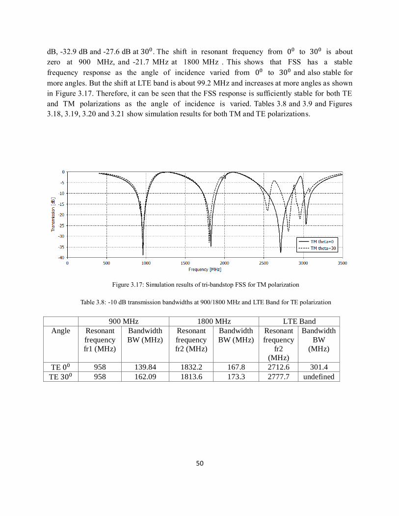
InFigure3.17,thetransmissionandreflectioncoefficientsarepresentedforTMpolarizationfor
and3 angleofincidence.Theresonant frequenciesat are961.1MHz,1826MHzand
2712.6MHz,whileat3 , theseare961.1MHz,1804.3MHzand2811.8MHz, respectively.
Thecorrespondingtransmissioncoefficientsare -38.7dB,-34.8dBand-37dBat ,and-36.9
50
dB,-32.9dBand-27.6dBat3 .Theshiftinresonantfrequencyfrom to3 isabout
zero at 900 MHz, and -21.7MHz at 1800MHz .This shows that FSS has a stable
frequencyresponseastheangleofincidencevariedfrom to3 andalsostablefor
moreangles.ButtheshiftatLTEbandisabout99.2MHzandincreasesatmoreanglesasshown
inFigure3.17.Therefore,itcanbeseenthattheFSSresponseissufficientlystableforbothTE
andTMpolarizationsastheangleofincidenceis varied.Tables3.8and3.9andFigures
3.18,3.19,3.20and3.21showsimulationresultsforbothTMandTEpolarizations.
Figure 3.17:Simulationresultsoftri-bandstopFSSforTMpolarization
Table 3.8:-10dBtransmissionbandwidthsat900/1800MHzandLTEBandforTEpolarization
900 MHz 1800 MHz LTE Band
Angle Resonant
frequency
fr1 (MHz)
Bandwidth
BW (MHz)
Resonant
frequency
fr2 (MHz)
Bandwidth
BW (MHz)
Resonant
frequency
fr2
(MHz)
Bandwidth
BW
(MHz)
TE 958 139.84 1832.2 167.8 2712.6 301.4
TE 3 958 162.09 1813.6 173.3 2777.7 undefined
51
Figure 3.18:transmissionbandwidthsat900/1800MHzandLTEBandforTEpolarizationattheta=0
Figure 3.19:transmissionbandwidthsat900/1800MHzandLTEBandforTEpolarizationattheta=30
Table 3.9:-10dBtransmissionbandwidthsat900/1800MHzandLTEBandforTMpolarization
900 MHz 1800 MHz LTE Band
Angle Resonant
frequency
fr1 (MHz)
Bandwidth
BW (MHz)
Resonant
frequency
fr2 (MHz)
Bandwidth
BW (MHz)
Resonant
frequency
fr3
(MHz)
Bandwidth
BW
(MHz)
TM 961.1 143.1 1826 169.1 2712.6 310
TM 3 961.1 123.4 1804.3 138.2 2811.8 undefined

52
Figure 3.20:transmissionbandwidthsat900/1800MHzandLTEBandforTMpolarizationattheta=0
Figure 3.21:transmissionbandwidthsat900/1800MHzandLTEBandforTMpolarizationattheta=30
3.7 Quad bandstop E_shape FSS:
The fourthdesign foranFSSstructure ispresentedinFigure3.22.Itisdesignedtocover four
bandsGSM900,GSM1800,3GandLTEatnormalincidence.
3.7.1 Structure of FSS:
The unit cell dimensions of bandstop FSS are shown in Figure 3.22. The bandstop
characteristics are achieved by designing several elements of different dimensions on FR-4

53
substrate.The thickness of FR-4substrate is 3.2mmand the relative permittivity (𝜀𝑟) and the
losstangent(tanδ)are4.3and0.02,respectively.Theperiodicityofunitcellis63.5×63.5mm .
Thecircumferenceoftheoutersquareopenloopelementis103.9mmwhichistunedto900
MHzwhiletheotherdimensionsofthestructurearetunedto1800MHz,3GandLTEband.
Thewidthofallmicrostripelementsis1.9mm.ThedimensionsoftheFSSstructurearedepicted
intable3.10.
Figure 3.22: overall view of the unit cell model
Figure 3.23:a)dimensionsoftopviewmodel,b)sideviewofthemodel

54
Table 3.10:dimensionsofthedesign
Name A B C D F
Value (mm) 55.31 35.42 30.95 15.43 26.76
Name K w g h t Value (mm) 3.56 2.4 1.15 3.2 0. 1
3.7.2 Simulation results: Theunit cellofFSSis showninFigure3.24.The transmissionandreflection coefficients
areobtainedfrom400-3000MHzforbothTEandTMpolarizationsatnormalincidence.
Figure 3.24:periodiccells
In Figure 3.25, the transmission and reflection coefficients are presented for TE polarization
normal incidence.The resonant frequencies are 922.6MHz (forGSM900), 2048.4MHz (for

55
GSM1800and3G)and2591.8MHz(forLTE).Thecorrespondingtransmissioncoefficientsare
-24.5dB,-34.2dB,-25.2dBrespectively.
Figure 3.25:Simulationresultsofquad-bandstopFSSforTEpolarization
3.7.3 The effect of changing the widths of elements: AsshowninFigure3.26,thebandwidthandresonantfrequencyofthefirstband(900MHz)is
stillstablewithvaryingtheelementswidthfrom2mmto2.5mm.Butthisvariationenhancethe
bandwidthof1800MHz/3Gbandfrom355MHzatwi=2mmto403MHzatwi=2.5mm.Inthe
lastband(LTE)thebandwidthisalmostfixed,buttheresonantfrequencyincreasesfrom2563.2
MHzatwi=2mmto2591.8MHzatwi=2.5mm.
Figure 3.26:Simulationresultsofquad-bandstopFSSforTEpolarizationwithvaryingtheelementswidth
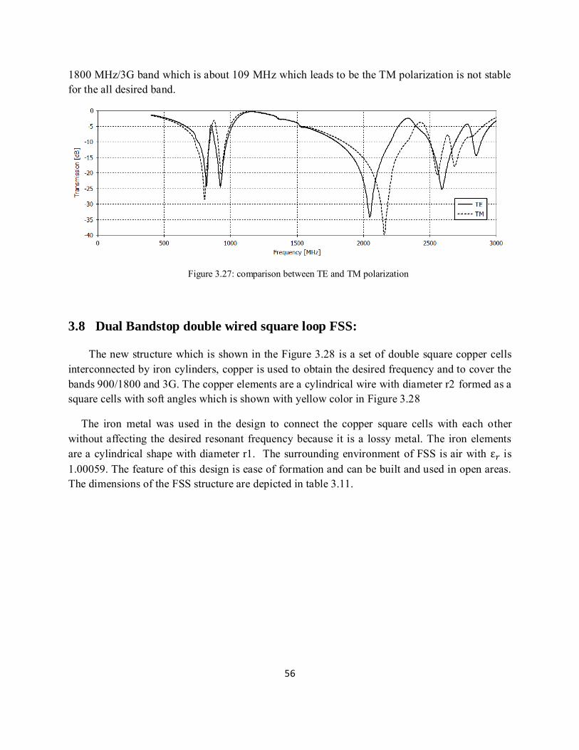
From comparison of TE polarization with TM polarization shown in Figure 3.27, we
noticetheshiftinginresonantfrequencyin900MHzbandwith8MHz,buttheshiftisbiggerin
56
1800MHz/3Gbandwhichisabout109MHzwhichleadstobetheTMpolarizationisnotstable
forthealldesiredband.
Figure 3.27:comparisonbetweenTEandTMpolarization
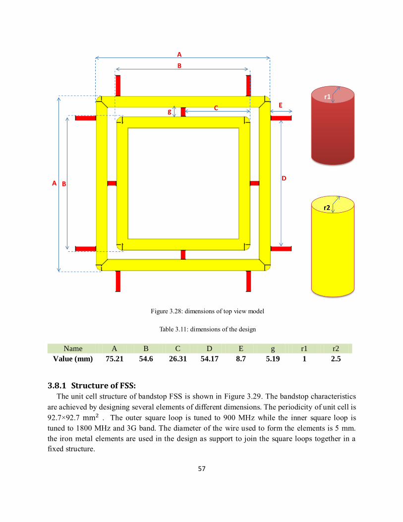
3.8 Dual Bandstop double wired square loop FSS:
ThenewstructurewhichisshownintheFigure3.28isasetofdoublesquarecoppercells
interconnectedbyironcylinders,copperisusedtoobtainthedesiredfrequencyandtocoverthe
bands900/1800and3G.Thecopperelementsareacylindricalwirewithdiameterr2formedasa
squarecellswithsoftangleswhichisshownwithyellowcolorinFigure3.28
The iron metal was used in the design to connect the copper square cells with each other
withoutaffectingthedesiredresonant frequencybecauseitisa lossymetal.Theironelements
areacylindricalshapewithdiameterr1. ThesurroundingenvironmentofFSSisairwithε𝑟is
1.00059.Thefeatureofthisdesigniseaseofformationandcanbebuiltandusedinopenareas.
ThedimensionsoftheFSSstructurearedepictedintable3.11.
57
Figure 3.28:dimensionsoftopviewmodel
Table 3.11:dimensionsofthedesign
Name A B C D E g r1 r2
Value (mm) 75.21 54.6 26.31 54.17 8.7 5.19 1 2.5
3.8.1 Structure of FSS: TheunitcellstructureofbandstopFSSisshowninFigure3.29.Thebandstopcharacteristics
areachievedbydesigningseveralelementsofdifferentdimensions.Theperiodicityofunitcellis
92.7×92.7mm . Theouter square loop is tuned to900MHzwhile the inner square loop is
tunedto1800MHzand3Gband.Thediameterofthewireusedtoformtheelementsis5mm.
theironmetal elementsareusedinthedesignas supporttojointhe squareloops togetherina
fixedstructure.

58
Figure 3.29:periodicsquarecells
3.8.2 Simulation results:
The transmissionand reflection coefficients are obtained from 400 to2600 MHz for
bothTEandTMpolarizations.
InFigure3.30,thetransmissionandreflectioncoefficientsarepresented forTEpolarization
for and3 angle of incidence.The resonant frequenciesat are972.4MHzand1994.8
MHz, while at 3 , these are 965.2 MHz and 1973.2 MHz respectively. The corresponding
transmissioncoefficientsare-55.4dB,-58.1dBat ,and-54dB,-59.7dBat3 .Theshiftin
resonant frequency from to3 is about -7.2MHzat 900MHz.and -21.6MHzat
1800MHz/3G This shows that FSS has a stable frequency response as the angle of
incidencevariedfrom to3 .

59
Figure 3.30:Simulationresultsoftri-bandstopFSSforTEpolarization
InFigure3.31,thetransmissionandreflectioncoefficientsarepresentedforTMpolarizationfor
and 3 angle of incidence.The resonant frequencies at are 972.4MHz, 1994.8MHz,
whileat3 , theseare990.4MHz,1926.4MHz.The corresponding transmission coefficients
are-52.5dB,-58.7dBat ,and-52.4dB,-57.5dBat3 ,respectively.Theshiftinresonant
frequencyfrom to3 isabout18MHzat900MHz,and-68.4MHzat1800MHz/3G
ThisshowsthatFSShasastablefrequencyresponseastheangleofincidencevaried
from to3 .Therefore,itcanbeseenthattheFSSresponseissufficientlystableforboth
TEandTMpolarizationsastheangleofincidenceisvaried.
Figure 3.31:Simulationresultsoftri-bandstopFSSforTMpolarization
Figures 3.32 and 3.33 show that the resonant frequencies are stable over TE and TM
polarizations,butwhentheangleincreasesto3 theresonantfrequenciesshiftedby25.2MHz
at band 900MHz, and shifted by -46.8 MHz at band 1800/3G. Tables 3.12 and 3.13 show
simulationresultsforbothTMandTEpolarizations.

60
Figure 3.32:TEandTMpolarizationattheta=0
Figure 3.33:TEandTMpolarizationattheta=40
Table 3.12:-10dBtransmissionbandwidthsat900/1800MHzand3GBandforTEpolarization
900 MHz 1800 MHz/3G
Angle Resonant frequency
fr1 (MHz)
Bandwidth
BW (MHz)
Resonant frequency
fr2 (MHz)
Bandwidth
BW (MHz)
TE 972.4 225.3 1994.8 639.8
TE 3 965.2 226.4 1973.2 503
Table 3.13:-10dBtransmissionbandwidthsat900/1800MHzandLTEBandforTMpolarization
900 MHz 1800 MHz
Angle Resonant frequency
fr1 (MHz)
Bandwidth
BW (MHz)
Resonant frequency
fr2 (MHz)
Bandwidth
BW (MHz)
TM 972.4 221 1994.8 626
TM 3 990.4 186 1926.4 478

61
Chapter 4: Conclusion
4.1 Summary:
The main purpose of this project is the analysis and design of microstrip frequency selective
surfaces and wire net structures to shield the GSM frequencies and transmit the other
frequencies.Theotherpurposesthataddedtoincludeothermobilesystemssuchas3GandLTE.
New five structuresare designed.The FSSsarealmostunchangedwhen the incidentangle is
increased from to3 forbothTEandTMpolarizations.Tables from4.1 to4.9 show the
transmissioncoefficientsatdesiredfrequenciesoftheproject.
4.1.1 First design (Bandstop double square loop FSS): Table4.1and4.2showthatthedeferenceins betweenTEandTMpolarizationlittleatdesired
frequencyandtheresultisstablewhentheincidentanglechangesfromzeroto45
Table 4.1:s (dB)atdesiredfrequenciesattheta=
GSM 900 GSM 1800
925 MHz 960 MHz 1805 MHz 1880 MHz
TE 𝟎𝟎 -23 -16 -32 -24
TM𝟎𝟎 -24 -15 -32 -24
Table 4.2:Table1:s (dB)atdesiredfrequenciesattheta=45
GSM 900 GSM 1800
925 MHz 960 MHz 1805 MHz 1880 MHz
TE 𝟓𝟎 -22 -18 -20 -19
TM 𝟓𝟎 -15 -17 -20 -12
4.1.2 Second design (Tri bandstop open loop FSS with FR substrate):
Weshowthatthetransmissioncoefficientsisstableoverthethreerequiredbandsattheta= as
shownintable4.3,buttherequiredresultsnotvalidwhenthetachangesto3 atLTEbandas
showninTable4.4.
Table 4.3:s (dB)atdesiredfrequenciesattheta=
GSM 900 GSM 1800 LTE
925 MHz 960 MHz 1805 MHz 1880 MHz 2620 MHz 2690 MHz
TE 𝟎𝟎 -20.2 -16.2 -26.9 -13.2 -13.7 -20.7
TM 𝟎𝟎 -19.8 -16 -25.3 -14 -13.7 -20.9

62
Table 4.4:s (dB)atdesiredfrequenciesattheta=3
GSM 900 GSM 1800 LTE
925 MHz 960 MHz 1805 MHz 1880 MHz 2620 MHz 2690 MHz
TE 𝟎𝟎 -20.3 -18.5 -23.5 -15.4 -15 -8.3
TM 𝟎𝟎 -18.5 -15.5 -27 -12 -14 -7.6
4.1.3 Third design (Tri bandstop open loop FSS with glass (pyrex) substrate) It showninTable4.5the stabilityandgoodresultsof the transmission coefficientsatthethree
requiredbandswhentheta= ,butwhenthetachangesto3 theLTEbandbecamenotstable
andtherequireds atallGSM1800bandnotvalidasshowninTable4.6.
Table 4.5:s (dB)atdesiredfrequenciesattheta=
GSM 900 GSM 1800 LTE
925 MHz 960 MHz 1805 MHz 1880 MHz 2620 MHz 2690 MHz
TE 𝟎𝟎 -17.1 -35.3 -20.18 -13.9 -15 -26.3
TM 𝟎𝟎 -16.5 -37.6 -22.5 -12.5 -15.1 -26.8
Table 4.6:s (dB)atdesiredfrequenciesattheta=3
GSM 900 GSM 1800 LTE
925 MHz 960 MHz 1805 MHz 1880 MHz 2620 MHz 2690 MHz
TE 𝟎𝟎 -17.5 -34.8 -29.7 -11.2 -8.6 -12.4
TM 𝟎𝟎 -13.8 -35.4 -32.3 -8 -4.2 -7.2
4.1.4 Fourth design (Quad bandstop E_shape FSS) In this design it is illustrated as shown inTable 4.7 that the good results achieved over four
mobilebandsatTEpolarizationwhentheta= ,therequireds resultsatTMpolarizationnot
validatfrequencies1805MHzand2620MHz.
Table 4.7:s (dB)atdesiredfrequenciesattheta=
GSM 900 GSM 1800 3G LTE
925
MHz
960
MHz
1805
MHz
1880
MHz
2110
MHz
2170
MHz
2620
MHz
2690
MHz
TE 𝟎𝟎 -24 -12.2 -10.2 -13 -19 -12.6 -20 -10.2
TM 𝟎𝟎 -20 -10.3 -9 -11 -25 -35 -8.7 -17.7
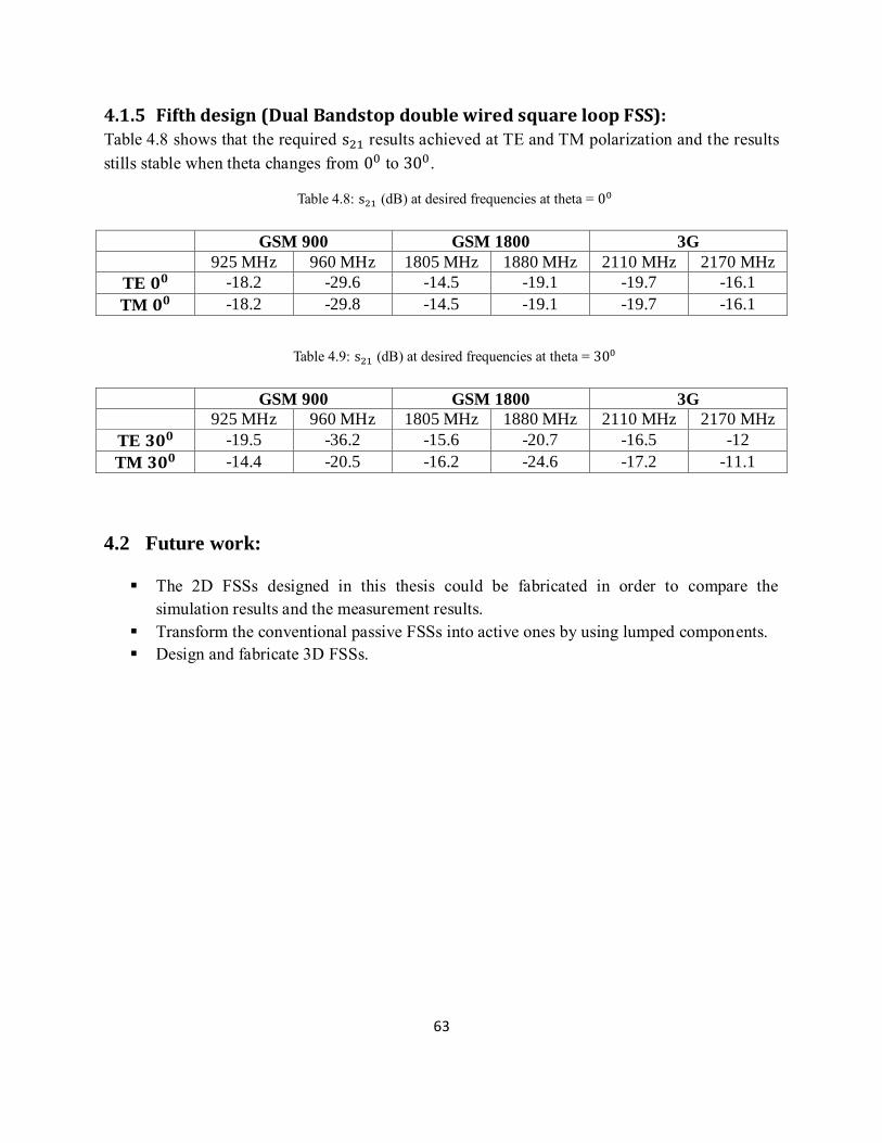
63
4.1.5 Fifth design (Dual Bandstop double wired square loop FSS):
Table4.8showsthattherequireds resultsachievedatTEandTMpolarizationandtheresults
stillsstablewhenthetachangesfrom to3 .
Table 4.8:s (dB)atdesiredfrequenciesattheta=
GSM 900 GSM 1800 3G
925 MHz 960 MHz 1805 MHz 1880 MHz 2110 MHz 2170 MHz
TE 𝟎𝟎 -18.2 -29.6 -14.5 -19.1 -19.7 -16.1
TM 𝟎𝟎 -18.2 -29.8 -14.5 -19.1 -19.7 -16.1
Table 4.9:s (dB)atdesiredfrequenciesattheta=3
GSM 900 GSM 1800 3G
925 MHz 960 MHz 1805 MHz 1880 MHz 2110 MHz 2170 MHz
TE 𝟎𝟎 -19.5 -36.2 -15.6 -20.7 -16.5 -12
TM 𝟎𝟎 -14.4 -20.5 -16.2 -24.6 -17.2 -11.1
4.2 Future work:
The 2D FSSs designed in this thesis could be fabricated in order to compare the
simulationresultsandthemeasurementresults.
TransformtheconventionalpassiveFSSsintoactiveonesbyusinglumpedcomponents.
Designandfabricate3DFSSs.
64
References
[1] D.Hu,“Introduction,”in 3D Frequency Selective Surfaces, vol. 98, Sheffield , United
Kingdom, 2012, pp. 1–2.
[2] A. Munir, V. Fusco and O. Malyuskin, 'Tunable Frequency Selective Surfaces
Characterisation', 2008 38th European Microwave Conference, 2008.
[3] Haiyan Chen, Xinyu Hou and Longjiang Deng, 'Design of Frequency-Selective Surfaces
Radome for a Planar Slotted Waveguide Antenna', Antennas Wirel. Propag. Lett., vol. 8, pp.
1231-1233, 2009.
[4] G. Kiani and V. Dyadyuk, 'Low loss FSS polarizer for 70 GHz applications', Proceedings of
the 2012 IEEE International Symposium on Antennas and Propagation, 2012.
[5] K. R. Jha, G. Singh, and R. Jyoti,“ A simple synthesis technique of single square loop
frequency selective surface” Progress In Electromagnetics Research B, vol. 45, pp. 165–185,
2012.
[6] R. Dickie, R. Cahill, V. Fusco, H. Gamble and N. Mitchell, 'THz Frequency Selective
Surface Filters for Earth Observation Remote Sensing Instruments', IEEE Transactions on
Terahertz Science and Technology, vol. 1, no. 2, pp. 450-461, 2011.
[7] R. Dickie, R. Cahill, H. Gamble, V. Fusco, B. Moyna, P. Huggard, N. Grant and C.
Philpot, 'Micromachined 300 GHz high Q resonant slot frequency selective surface filter', IEE
Proceedings - Microwaves, Antennas and Propagation, vol. 151, no. 1, p. 31, 2004.
[8] Wikipedia, "1G", 2015. [Online]. Available: https://en.wikipedia.org/wiki/1G. [Accessed: 26-
Dec- 2015].
[9] Wikipedia, "History of mobile phones", 2015. [Online]. Available:
https://en.wikipedia.org/wiki/History_of_mobile_phones. [Accessed: 26- Dec- 2015].
[10] Globalspec.com, "Chapter 2: First Generation Analog Cellular | IHS Engineering360",
2015. [Online]. Available: http://www.globalspec.com/reference/52290/203279/chapter-2-first-
generation-analog-cellular. [Accessed: 26- Dec- 2015].
[11] L. Aravamudhan, S. Faccin, R. Mononen, B. Patil, Y. Saifullah, S. Sharma and S.
Sreemanthula, 'Second-Generation Mobile Networks | Getting to Know Wireless Networks and
Technology | InformIT', Informit.com, 2015. [Online]. Available:
http://www.informit.com/articles/article.aspx?p=98132&seqNum=4. [Accessed: 19- Nov- 2015].
65
[12] Slideshare.net, "Introduction to 3 g mobile communications (juha korhonen)", 2015.
[Online]. Available: http://www.slideshare.net/tbutomo/introduction-to-3-g-mobile-
communications-juha-korhonen. [Accessed: 26- Dec- 2015].
[13] A. Singh, "GSM & CDMA", Slideshare.net, 2015. [Online]. Available:
http://www.slideshare.net/abhijeetsinghims/gsm-cdma-52837157. [Accessed: 26- Dec- 2015].
[14] Wikipedia, '3G', 2015. [Online]. Available: https://en.wikipedia.org/wiki/3G. [Accessed: 28-
Nov- 2015].
[15] Arcelect.com, '2G - 3G Cellular Wireless GSM, GPRS, EDGE, W-
CDMA, UMTS, TDMA, CDMA, CDMA2000 1xRTT, CDMA2000 1xEV-DO, and
CDMA2000 1xEV-DV', 2015. [Online]. Available: http://www.arcelect.com/2G-
3G_Cellular_Wireless.htm. [Accessed: 20- Nov- 2015].
[16] T. Zacharopoulou, 'Why LTE is a success? LTE vs WiMAX', 0el70lte, 2012. [Online].
Available: https://0el70lte.wordpress.com/2012/06/29/why-lte-is-a-success-lte-vs-wimax/.
[Accessed: 23- Nov- 2015].
[17] 4gamericas.org, '4gamericas :: Statistics - Global', 2015. [Online]. Available:
http://www.4gamericas.org/en/resources/statistics/statistics-global/. [Accessed: 23- Nov- 2015].
[18] Molisch, Andreas (2010). Wireless communications(2. ed.). Oxford: Wiley- Blackwell.
p. 591. ISBN 978-0-470-74186-3. Retrieved 29 January 2015
[19] Worldtimezone.com, 'GSM World Coverage Map- GSM Country List by frequency bands',
2015. [Online]. Available: http://www.worldtimezone.com/gsm.html. [Accessed: 27- Nov-
2015].
[20] Radio-electronics.com, 'UMTS Frequency Bands | 3G WCDMA UARFCN | Radio-
Electronics.Com', 2015. [Online]. Available: http://www.radio-
electronics.com/info/cellulartelecomms/umts/umts-wcdma-frequency-bands-frequencies.php.
[Accessed: 28- Nov- 2015].
[21] Radio-electronics.com, 'LTE Bands | LTE Frequency Bands Spectrum | Radio-
Electronics.com', 2015. [Online]. Available: http://www.radio-
electronics.com/info/cellulartelecomms/lte-long-term-evolution/lte-frequency-spectrum.php.
[Accessed: 28- Nov- 2015].
66
[22] Spectrummonitoring.com, 'List of Mobile Frequencies by Country (GSM, CDMA, UMTS,
LTE)', 2015. [Online]. Available: http://www.spectrummonitoring.com/frequencies/. [Accessed:
28- Nov- 2015].
[23] Gsmarena.com, 'Network coverage in Israel - 2G/3G/4G mobile networks', 2015. [Online].
Available: http://www.gsmarena.com/network-bands.php3?sCountry=Israel. [Accessed: 28-
Nov- 2015].
[24] F. Costa, A. Monorchio and G. Manara, "An Overview of Equivalent Circuit Modeling
Techniques of Frequency Selective Surfaces and Metasurfaces", Applied Computational
Electromagnetics Society Journal, vol. 29, no. 12, 2014.
[25]K.SarabandiandN.Behdad,“Afrequencyselectivesurfacewithminiaturizedelements,”
IEEE Trans. Antennas Propag., vol. 55, pp. 1239-1245, May 2007.
[26]B.Hooberman,“Everything you ever wanted to know about frequency-selective surface
filtersbutwereafraidtoask,”May,2005.
http://calvin.phys.columbia.edu/group_web/filter_development/download/filter.pdf and
http://calvin.phys.columbia.edu/group_web/filter_development/download/References.pdf
[27] C. Lee and R. Langley, 'Equivalent-circuit models for frequency-selective surfaces at
oblique angles of incidence', IEE Proc. H Microw. Antennas Propag. UK, vol. 132, no. 6, p. 395,
1985.
[28] MARCUVITZ , N. : 'Waveguide handbook ' (McGraw-Hill , 1951)
[29] R. Langley and E. Parker, 'Equivalent circuit model for arrays of square loops', Electron.
Lett., vol. 18, no. 7, p. 294, 1982.
[30] Academia.edu, 'A New Equivalent Circuit Based FSS Design Method by Using Genetic
Algorithm', 2015. [Online]. Available:
https://www.academia.edu/723002/A_New_Equivalent_Circuit_Based_FSS_Design_Method_by
_Using_Genetic_Algorithm. [Accessed: 11- Dec- 2015].
[31] W. Che, H. Ye, Y. Xiong, Y. Chang and C. Christopoulos, 'A fast and efficient method
for design of circuit analog absorbers consisting of resistive square loop arrays', 2015 IEEE
International Conference on Computational Electromagnetics, 2015.

67
[32] A. Campos and T. Silva, 'Spectral domain analysis of double screen frequency selective
surfaces', Journal of Microwaves, Optoelectronics and Electromagnetic Applications, vol. 11, no.
1, pp. 81-92, 2012.
[33] A. Campos, R. Moreira and J. Trindade, "A comparison between the equivalent circuit
model and moment method to analyze FSS", 2009 SBMO/IEEE MTT-S International
Microwave and Optoelectronics Conference (IMOC), 2009.
[34] M. Hosseini and M. Hakkak, "Characteristics Estimation for Jerusalem Cross-Based
Artificial Magnetic Conductors", Antennas Wirel. Propag. Lett., vol. 7, pp. 58-61, 2008.
[35] D. Singh, A. Kumar, S. Meena and V. Agrawala, " Analysis of frequency selective
surfaces for radar absorbing materials ", Progress In Electromagnetics Research B, vol. 38, pp.
297-314, 2012.
[36] M. Aziz, M. Shukor, B. Ahmad, M. Suaidi, M. Johar, M. Othman, S. Salleh, F. Azmin
and M. Malek, "Investigation of a square loop Frequency Selective Surface (FSS) on hybrid
material at 2.4 GHz", 2013 IEEE International Conference on Control System, Computing and
Engineering, 2013.
[37] M. Raspopoulos and S. Stavrou, "Frequency Selective Buildings Through Frequency
Selective Surfaces", IEEE Trans. Antennas Propagat., vol. 59, no. 8, pp. 2998-3005, 2011.
[38] G. Sen, T. Mandal, S. Majumdar, S. Mahato, S. Mondal and P. Sarkar, "Design of a
wide band Frequency Selective Surface (FSS) for multiband operation of reflector antenna",
2012 5th International Conference on Computers and Devices for Communication (CODEC),
2012.
[39] E. Yildirim and O. Civi, "Design of a wideband radar absorbing structure", Antennas and
Propagation (EUCAP), Proceedings of the 5th European Conference on, pp. 1324-1327, 2011.
[40] T. Zhang, G. Yang, W. Li, Q. Jiang and Q. Wu, "Research on novel miniaturized
frequency selective surfaces consist of rectangle spiral-based elements", 2010 Global Mobile
Congress, 2010.
[41] Hui Lai Liu, K. Ford and R. Langley, "Design Methodology for a Miniaturized Frequency
Selective Surface Using Lumped Reactive Components", IEEE Trans. Antennas Propagat., vol.
57, no. 9, pp. 2732-2738, 2009.
[42] Connection.ebscohost.com, "Selective Control of GSM 900 MHz, GSM 1800 MHz and
ISM 2.4 GHz Communication inside Room using Tri-Band Jerusalem Cross Frequency Selective

68
Wall", 2015. [Online]. Available: http://connection.ebscohost.com/c/articles/99720180/selective-
control-gsm-900-mhz-gsm-1800-mhz-ism-2-4-ghz-communication-inside-room-using-tri-band-
jerusalem-cross-frequency-selective-wall. [Accessed: 18- Dec- 2015].
[43] E. Unal, A. Gokcen and Y. Kutlu, "Effective electromagnetic shielding", IEEE Microwave
Magazine, vol. 7, no. 4, pp. 48-54, 2006.
[44] Cst.com, "CST - Computer Simulation Technology", 2016. [Online]. Available:
https://www.cst.com/. [Accessed: 08- Jan- 2016].