Design of a two-bar truss: optimization and uncertainty...
13
Design of a two-bar truss: optimization and uncertainty propagation CEE 201L. Uncertainty, Design, and Optimization Department of Civil and Environmental Engineering Duke University Jeffrey T. Scruggs and Henri P. Gavin Spring, 2014 Consider a statically-determinate two-bar truss loaded by a horizontal load F . The lengths of bars 1 and 2 depend on the locations of joints 1 and 2. L 1 = X 2 1 + Y 2 1 = (x 1 - x 3 ) 2 +(y 1 - y 3 ) 2 = x 2 1 + h 2 L 2 = X 2 2 + Y 2 2 = (x 2 - x 1 ) 2 +(y 1 - y 2 ) 2 = (x 2 - x 1 ) 2 + h 2 where X i and Y i are the positive-valued x-axis and y-axis projections of the inclined bars. R R R T joint 3 (0,0) 3y 3x R F 2y 2x joint 2 (x , h) 1 joint 1 2 (x , 0) bar 1 bar 2 1 2 T Design Analysis In truss analysis, there are 2J independent equilibrium equations and B +R unknowns, where J is the number of joints, B is the number of bars, and R is the number of external reaction forces. If 2J = B + R, the truss is statically determinate. (The number of equilibrium equations equals the number of unknowns.)
-
Upload
truongdien -
Category
Documents
-
view
218 -
download
1
Transcript of Design of a two-bar truss: optimization and uncertainty...

Design of a two-bar truss:optimization and uncertainty propagation
CEE 201L. Uncertainty, Design, and OptimizationDepartment of Civil and Environmental Engineering
Duke University
Jeffrey T. Scruggs and Henri P. GavinSpring, 2014
Consider a statically-determinate two-bar truss loaded by a horizontal load F . The lengthsof bars 1 and 2 depend on the locations of joints 1 and 2.
L1 =√X2
1 + Y 21 =
√(x1 − x3)2 + (y1 − y3)2 =
√x2
1 + h2
L2 =√X2
2 + Y 22 =
√(x2 − x1)2 + (y1 − y2)2 =
√(x2 − x1)2 + h2
where Xi and Yi are the positive-valued x-axis and y-axis projections of the inclined bars.
��������������������
��������������������
R R
R
T
joint 3(0,0)
3y
3xR
F
2y
2x
joint 2
(x , h)1
joint 1
2(x , 0)
bar 1
bar 2
1 2T
Design Analysis
In truss analysis, there are 2J independent equilibrium equations and B+R unknowns, whereJ is the number of joints, B is the number of bars, and R is the number of external reactionforces. If 2J = B + R, the truss is statically determinate. (The number of equilibriumequations equals the number of unknowns.)

2 CEE 201L. Uncertainty, Design, and Optimization – Duke University – Spring 2014 – H.P. Gavin
The equilibrium equations at the loaded joint (joint 1) are+→∑
Fx = 0 : −c1T1 + c2T2 = F ,
+↑∑Fy = 0 : −s1T1 − s2T2 = 0 .
The equilibrium equations at joint 2 are+→∑
Fx = 0 : −c2T2 +R2x = 0 ,+↑∑Fy = 0 : s2T2 +R2y = 0 .
The equilibrium equations at joint 3 are+→∑
Fx = 0 : c1T1 +R3x = 0 ,+↑∑Fy = 0 : s1T1 +R3y = 0 ,
where ci = Xi/Li and si = Yi/Li.
The reaction forces may be found from equilibrium equations for the entire truss, and can beused as a check on the solution.
R2x +R3x = F
R2y +R3y = 0R2y x2 = −FhR3y x2 = Fh
If no errors were made in deriving the three pairs of joint equilibrium equations, the reactionforce equations are simply a linear combination of two or more of the other equations.
The bar tension and reaction forces may be found by solving the matrix equation
−c1 c2 0 0 0 0−s1 −s2 0 0 0 0
0 −c2 1 0 0 00 s2 0 1 0 0c1 0 0 0 1 0s1 0 0 0 0 10 0 1 0 1 00 0 0 1 0 10 0 0 x2 0 00 0 0 0 0 x2
T1T2R2xR2yR3xR3y
=
F00000F0−F hF h
Note that the first B columns of the matrix sum to zero. This is true for any truss analyzed inthis way and is simply a statement that each bar of the truss is in equilibrium with itself. Thelast four rows of the matrix and the right-hand-side vector represent the reaction equationsand need-not be included. They just provide more equations than unknowns, and can helpserve as a check on the equations.
CC BY-NC-ND J.T. Scruggs & H.P. Gavin
Optimization example: a two-bar truss 3
Design Goal
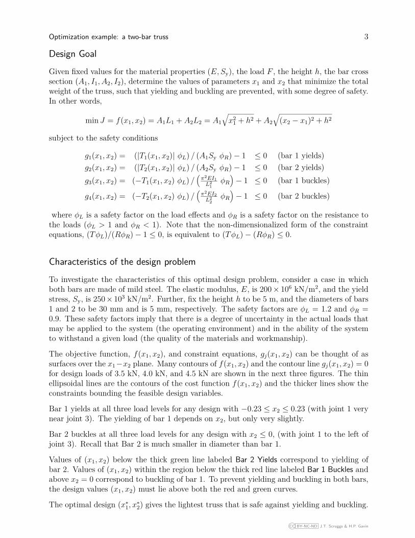
Given fixed values for the material properties (E, Sy), the load F , the height h, the bar crosssection (A1, I1, A2, I2), determine the values of parameters x1 and x2 that minimize the totalweight of the truss, such that yielding and buckling are prevented, with some degree of safety.In other words,
min J = f(x1, x2) = A1L1 + A2L2 = A1
√x2
1 + h2 + A2
√(x2 − x1)2 + h2
subject to the safety conditions
g1(x1, x2) = (|T1(x1, x2)| φL) / (A1Sy φR)− 1 ≤ 0 (bar 1 yields)g2(x1, x2) = (|T2(x1, x2)| φL) / (A2Sy φR)− 1 ≤ 0 (bar 2 yields)g3(x1, x2) = (−T1(x1, x2) φL) /
(π2EI1L2
1φR)− 1 ≤ 0 (bar 1 buckles)
g4(x1, x2) = (−T2(x1, x2) φL) /(π2EI2L2
2φR)− 1 ≤ 0 (bar 2 buckles)
where φL is a safety factor on the load effects and φR is a safety factor on the resistance tothe loads (φL > 1 and φR < 1). Note that the non-dimensionalized form of the constraintequations, (TφL)/(RφR)− 1 ≤ 0, is equivalent to (TφL)− (RφR) ≤ 0.
Characteristics of the design problem
To investigate the characteristics of this optimal design problem, consider a case in whichboth bars are made of mild steel. The elastic modulus, E, is 200× 106 kN/m2, and the yieldstress, Sy, is 250× 103 kN/m2. Further, fix the height h to be 5 m, and the diameters of bars1 and 2 to be 30 mm and is 5 mm, respectively. The safety factors are φL = 1.2 and φR =0.9. These safety factors imply that there is a degree of uncertainty in the actual loads thatmay be applied to the system (the operating environment) and in the ability of the systemto withstand a given load (the quality of the materials and workmanship).
The objective function, f(x1, x2), and constraint equations, gj(x1, x2) can be thought of assurfaces over the x1−x2 plane. Many contours of f(x1, x2) and the contour line gj(x1, x2) = 0for design loads of 3.5 kN, 4.0 kN, and 4.5 kN are shown in the next three figures. The thinellipsoidal lines are the contours of the cost function f(x1, x2) and the thicker lines show theconstraints bounding the feasible design variables.
Bar 1 yields at all three load levels for any design with −0.23 ≤ x2 ≤ 0.23 (with joint 1 verynear joint 3). The yielding of bar 1 depends on x2, but only very slightly.
Bar 2 buckles at all three load levels for any design with x2 ≤ 0, (with joint 1 to the left ofjoint 3). Recall that Bar 2 is much smaller in diameter than bar 1.
Values of (x1, x2) below the thick green line labeled Bar 2 Yields correspond to yielding ofbar 2. Values of (x1, x2) within the region below the thick red line labeled Bar 1 Buckles andabove x2 = 0 correspond to buckling of bar 1. To prevent yielding and buckling in both bars,the design values (x1, x2) must lie above both the red and green curves.
The optimal design (x∗1, x∗2) gives the lightest truss that is safe against yielding and buckling.
CC BY-NC-ND J.T. Scruggs & H.P. Gavin
4 CEE 201L. Uncertainty, Design, and Optimization – Duke University – Spring 2014 – H.P. Gavin
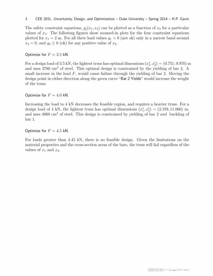
The safety constraint equations, gj(x1, x2) can be plotted as a function of x2 for a particularvalues of x1. The following figures show zoomed-in plots for the four constraint equationsplotted for x1 = 2 m. For all three load values g1 > 0 (not ok) only in a narrow band aroundx2 = 0, and g4 ≤ 0 (ok) for any positive value of x2.
Optimize for F = 3.5 kN.
For a design load of 3.5 kN, the lightest truss has optimal dimensions (x∗1, x∗2) = (0.751, 9.970) mand uses 3780 cm3 of steel. This optimal design is constrained by the yielding of bar 2. Asmall increase in the load F , would cause failure through the yielding of bar 2. Moving thedesign point in either direction along the green curve “Bar 2 Yields” would increase the weightof the truss.
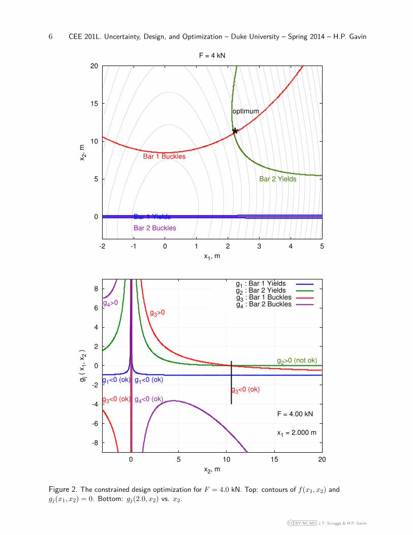
Optimize for F = 4.0 kN.
Increasing the load to 4 kN decreases the feasible region, and requires a heavier truss. For adesign load of 4 kN, the lightest truss has optimal dimensions (x∗1, x∗2) = (2.193, 11.060) m,and uses 4060 cm3 of steel. This design is constrained by yielding of bar 2 and buckling ofbar 1.
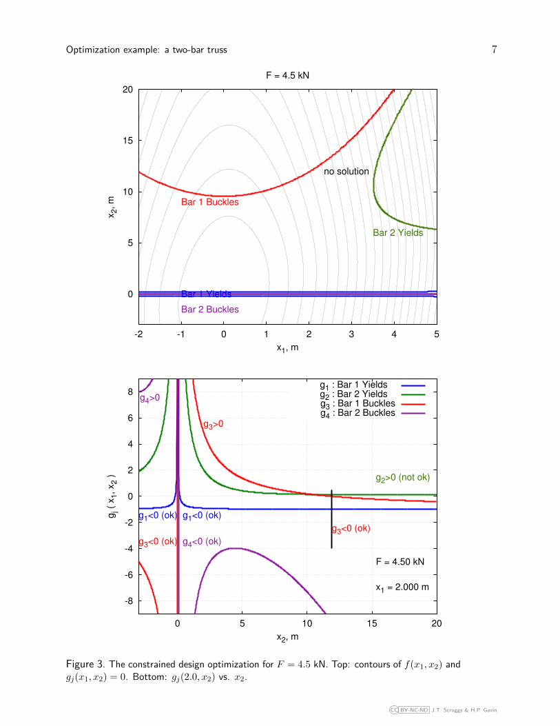
Optimize for F = 4.5 kN.
For loads greater than 4.45 kN, there is no feasible design. Given the limitations on thematerial properties and the cross-section areas of the bars, the truss will fail regardless of thevalues of x1 and x2.
CC BY-NC-ND J.T. Scruggs & H.P. Gavin

Optimization example: a two-bar truss 5
0
5
10
15
20
-2 -1 0 1 2 3 4 5
x2, m
x1, m
F = 3.5 kN
Bar 1 Yields
Bar 2 Buckles
Bar 2 Yields
Bar 1 Buckles
*optimum
-8
-6
-4
-2
0
2
4
6
8
0 5 10 15 20
gj (
x1, x
2 )
x2, m
g1 : Bar 1 Yields g2 : Bar 2 Yields g3 : Bar 1 Bucklesg4 : Bar 2 Buckles
F = 3.50 kN
x1 = 2.000 m
g1<0 (ok)g1<0 (ok)
g2<0 (ok)
g3<0 (ok)
g3>0
g3<0 (ok) g4<0 (ok)
g4>0
Figure 1. The constrained design optimization for F = 3.5 kN. Top: contours of f(x1, x2) andgj(x1, x2) = 0. Bottom: gj(2.0, x2) vs. x3.
CC BY-NC-ND J.T. Scruggs & H.P. Gavin
6 CEE 201L. Uncertainty, Design, and Optimization – Duke University – Spring 2014 – H.P. Gavin
0
5
10
15
20
-2 -1 0 1 2 3 4 5
x2, m
x1, m
F = 4 kN
Bar 1 Yields
Bar 2 Buckles
Bar 2 Yields
Bar 1 Buckles
*
optimum
-8
-6
-4
-2
0
2
4
6
8
0 5 10 15 20
gj (
x1, x
2 )
x2, m
g1 : Bar 1 Yields g2 : Bar 2 Yields g3 : Bar 1 Bucklesg4 : Bar 2 Buckles
F = 4.00 kN
x1 = 2.000 m
g1<0 (ok)g1<0 (ok)
g2>0 (not ok)
g3>0
g3<0 (ok)
g3<0 (ok) g4<0 (ok)
g4>0
Figure 2. The constrained design optimization for F = 4.0 kN. Top: contours of f(x1, x2) andgj(x1, x2) = 0. Bottom: gj(2.0, x2) vs. x2.
CC BY-NC-ND J.T. Scruggs & H.P. Gavin
Optimization example: a two-bar truss 7
0
5
10
15
20
-2 -1 0 1 2 3 4 5
x2, m
x1, m
F = 4.5 kN
Bar 1 Yields
Bar 2 Buckles
Bar 2 Yields
Bar 1 Buckles
no solution
-8
-6
-4
-2
0
2
4
6
8
0 5 10 15 20
gj (
x1, x
2 )
x2, m
g1 : Bar 1 Yields g2 : Bar 2 Yields g3 : Bar 1 Bucklesg4 : Bar 2 Buckles
F = 4.50 kN
x1 = 2.000 m
g1<0 (ok)g1<0 (ok)
g2>0 (not ok)
g3<0 (ok)
g3>0
g3<0 (ok) g4<0 (ok)
g4>0
Figure 3. The constrained design optimization for F = 4.5 kN. Top: contours of f(x1, x2) andgj(x1, x2) = 0. Bottom: gj(2.0, x2) vs. x2.
CC BY-NC-ND J.T. Scruggs & H.P. Gavin
8 CEE 201L. Uncertainty, Design, and Optimization – Duke University – Spring 2014 – H.P. Gavin
Safety Analysis
The safety constraints used in this design optimization incorporate a safety factor φL forthe truss bar loads and a safety factor φR for the resistance of the truss bars to these loads.A load factor φL > 1 makes the design safer by designing for larger-than-expected loads.A resistance factor φR < 1 makes the design safer by designing for weaker-than-expectedstrength/performance.
In most design situations the designer is uncertain as to the future “as-built” quality and theoperating environment of the designed system. The designer may also be uncertain as to theas-built quality of the designed system, when it is eventually produced. If the designer canestimate:
• an expected, average, or nominal load level (mean load, µL)
• the variability in the loads (standard deviation of the loads, σL)
• an expected, average, or nominal level of as-built quality(mean of the performance or resistance µR), and
• the variability in the as-built quality(standard deviation of the performance or resistance, σR)
then the designer can carry out a safety analysis to determine the probability of a productfailure. To do so, the safety of the optimized design is re-evaluated hundreds or thousands oftimes, each time using different randomly-generated values for the loading environment andthe strength characteristics. These randomly-generated loads and strengths will conform tothe designer’s expectation regarding the variability of the load and resistance.
For example, in this two-bar truss problem, a design is optimized using a load value of 3.5 kNand a strength value of 250 × 103 kN/m2. These values represent the designer’s expected(or mean or average) load, µL, and strength, µR, values. In the design of an adequately-safesystem, truss bar forces calculated on the basis of this expected load are multiplied by afactor φL of 1.2, and truss bar strengths calculated on the basis of this expected yield stressare multiplied by a factor φR of 0.9.
With an assessment of the variability in the loading environment, σL, and the strength, σR,the probability of failure of the optimized design (x∗1, x∗2) can be carried out as follows:
1. Generate random values for the parameters, x1 and x2, the load, F , and yield strength,Sy. These random values will have mean values and variances corresponding to thedesigner’s expectation of the loading environment, the strength properties of the man-ufactured product, and the manufacturing precision. The mean design parametersshould be the optimized values. The coefficient of variation for the design parameterscan be small (less than 5 percent).
2. Analyze the safety of the optimized design with the random values of x1, x2, F and Syusing φL = 1 and φR = 1 in the safety constraints (gj).
CC BY-NC-ND J.T. Scruggs & H.P. Gavin
Optimization example: a two-bar truss 9
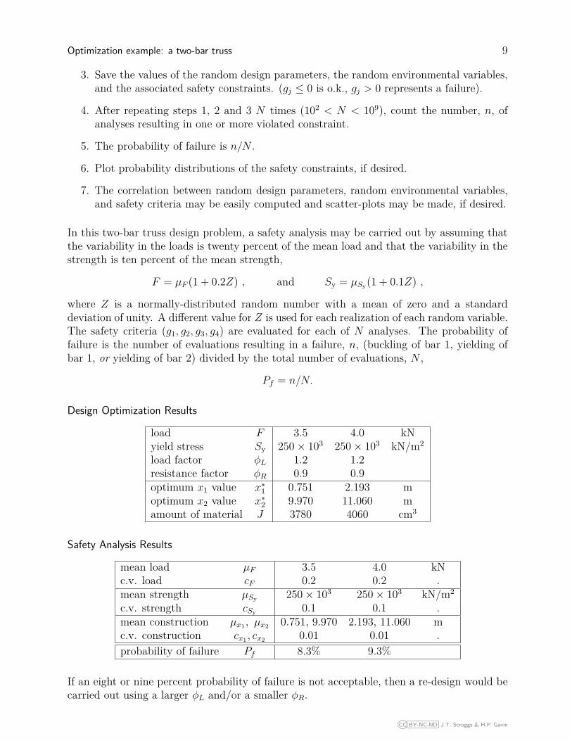
3. Save the values of the random design parameters, the random environmental variables,and the associated safety constraints. (gj ≤ 0 is o.k., gj > 0 represents a failure).
4. After repeating steps 1, 2 and 3 N times (102 < N < 109), count the number, n, ofanalyses resulting in one or more violated constraint.
5. The probability of failure is n/N .
6. Plot probability distributions of the safety constraints, if desired.
7. The correlation between random design parameters, random environmental variables,and safety criteria may be easily computed and scatter-plots may be made, if desired.
In this two-bar truss design problem, a safety analysis may be carried out by assuming thatthe variability in the loads is twenty percent of the mean load and that the variability in thestrength is ten percent of the mean strength,
F = µF (1 + 0.2Z) , and Sy = µSy(1 + 0.1Z) ,
where Z is a normally-distributed random number with a mean of zero and a standarddeviation of unity. A different value for Z is used for each realization of each random variable.The safety criteria (g1, g2, g3, g4) are evaluated for each of N analyses. The probability offailure is the number of evaluations resulting in a failure, n, (buckling of bar 1, yielding ofbar 1, or yielding of bar 2) divided by the total number of evaluations, N ,
Pf = n/N.
Design Optimization Results
load F 3.5 4.0 kNyield stress Sy 250× 103 250× 103 kN/m2
load factor φL 1.2 1.2resistance factor φR 0.9 0.9optimum x1 value x∗1 0.751 2.193 moptimum x2 value x∗2 9.970 11.060 mamount of material J 3780 4060 cm3
Safety Analysis Results
mean load µF 3.5 4.0 kNc.v. load cF 0.2 0.2 .mean strength µSy 250× 103 250× 103 kN/m2
c.v. strength cSy 0.1 0.1 .mean construction µx1 , µx2 0.751, 9.970 2.193, 11.060 mc.v. construction cx1 , cx2 0.01 0.01 .probability of failure Pf 8.3% 9.3%
If an eight or nine percent probability of failure is not acceptable, then a re-design would becarried out using a larger φL and/or a smaller φR.
CC BY-NC-ND J.T. Scruggs & H.P. Gavin

10 CEE 201L. Uncertainty, Design, and Optimization – Duke University – Spring 2014 – H.P. Gavin
Correlation Analysis Results
x1 x2 F Sy g1 g2 g3 g4x1 1.00 0.00 -0.05 -0.01 -0.04 -0.05 -0.03 0.08x2 0.00 1.00 -0.01 -0.04 -0.03 0.01 -0.06 -0.07F -0.05 -0.01 1.00 0.03 0.89 0.89 1.00 -1.00Sy -0.01 -0.04 0.03 1.00 -0.42 -0.42 0.03 -0.02g1 -0.04 -0.03 0.89 -0.42 1.00 1.00 0.89 -0.88g2 -0.05 0.01 0.89 -0.42 1.00 1.00 0.89 -0.89g3 -0.03 -0.06 1.00 0.03 0.89 0.89 1.00 -0.99g4 0.08 -0.07 -1.00 -0.02 -0.88 -0.89 -0.99 1.00
• Parameters x1 and x2 are most strongly correlated to g4 (buckling of bar 2), but thiscorrelation is weak and g4 is not active in the design, so small random variations in thedesign parameters do not affect safety.
• Load F is highly correlated to yielding failures, and is perfectly correlated to bucklingfailures. Increasing F makes both bars more likely to yield, bar 1 more likely to buckle,and bar 2 less likely to buckle.
• Strength Sy is moderately negatively correlated to yielding failures. As the yieldstrength increases, yielding failures tend to decrease.
• Constraints g1 and g2 (yielding of bars 1 and 2) are perfectly positively- correlated.
• Constraints g3 and g4 (buckling of bars 1 and 2) are perfectly negatively-correlated.
CC BY-NC-ND J.T. Scruggs & H.P. Gavin

Optimization example: a two-bar truss 11
Questions1. Check the equilibrium equations on pages 1 and 2 by drawing a free-body-diagram for
each of the three trusses in the joint.
2. Make a scaled drawing of the truss optimized for F = 3.5 kN and for F = 4.0 kN.Why are the bar angles more efficient for the 4.0 kN-optimized truss?If this geometry is more efficient for the 4.0 kN-optimized truss, why not use it for the3.5 kN-optimized truss as well?
3. What’s the deal with the constraints at x2 = 0?
4. For x2 < 0, why does it make sense that bar 2 will buckle and bar 3 will not? As partof your answer, draw a sketch of the truss in this configuration, indicate which bar is intension, and which is in compression, and make use of the known (given) bar diameters.
5. Why does it make sense that bar 2 will never buckle if x2 > 0?
6. At an optimal design point constrained by a single inequality (e.g., the design optimiza-tion for F = 3.5 kN), the contour of g = 0 and the contour of the cost function, f , aretangent to each other. This is a mathematical condition for the constrained optimum.(Moving along the constraint curve from the optimum point can only increase the cost.)Looking at the top part of Figure 1, does this appear to be the case in this problem?
7. The constraint for bar 1 yielding, g1, is nearly -1 for almost every possible design.Looking at the equations for the inequality constraints on page 3, could g1 possiblyever be less than -1? Physically, what does it mean that g1 is practically equal to -1?
8. The constraint for bar 2 buckling, g4, becomes very negative for x2 > 0. What does avery negative value for g4 represent, physically?
9. When carrying out a safety analysis to compute the probability of failure, why shouldsafety constraints (gj) be analyzed with safety factors set equal to 1 (φL = 1;φR = 1)?
10. Figures 4 and 6 show three distributions, as histograms and CDFs. Why do the distri-butions for the yielding of bar 1 (the blue line) have values only for g ≈ −1.
11. For the design optimized for F = 3.5 kN, is the truss more likely to fail from bar 2yielding or bar 1 buckling? Explain your answer using information from Figure 1.
12. For the design optimized for F = 4.0 kN, is the truss more likely to fail from bar 2yielding or bar 1 buckling? Explain your answer using information from Figure 2.
13. For the design optimized for F = 4.0 kN, which Lagrange multiplier would you expectto be larger, λ2 or λ3? Explain your answer using information from Figure 2.
14. Which change would reduce the failure probability for the F = 4.0 design more:(a) re-optimizing with φL = 0.90 and φR = 1.44, or(b) re-optimizing with φL = 0.81 and φR = 1.20?Why? Use information from Figure 7 in your answer.
CC BY-NC-ND J.T. Scruggs & H.P. Gavin

12 CEE 201L. Uncertainty, Design, and Optimization – Duke University – Spring 2014 – H.P. Gavin
0
0.2
0.4
0.6
0.8
1
-1 -0.8 -0.6 -0.4 -0.2 0 0.2 0.4
cum
ula
tive p
robabili
ty
constraint value, g
yielding of bar 1yielding of bar 2
buckling of bar 1
0
0.02
0.04
0.06
0.08
0.1
-1 -0.8 -0.6 -0.4 -0.2 0 0.2 0.4
his
togra
m
constraint value, g
yielding of bar 1yielding of bar 2
buckling of bar 1
Figure 4. Probability distribution plots of three of the safety criteria for F = 3.5 kN.
-1
-0.8
-0.6
-0.4
-0.2
0
150 200 250 300 350
bucklin
g o
f bar
1, g
3
yield stress, Sy, MPa
correlation = 0.03
-1
-0.8
-0.6
-0.4
-0.2
0
1 2 3 4 5 6
bucklin
g o
f bar
1, g
3
applied force, F, kN
correlation = 1.00
-0.8
-0.6
-0.4
-0.2
0
0.2
0.4
0.6
0.8
150 200 250 300 350
yie
ldin
g o
f bar
2, g
2
yield stress, Sy, MPa
correlation = -0.42
-0.8
-0.6
-0.4
-0.2
0
0.2
0.4
0.6
0.8
1 2 3 4 5 6
yie
ldin
g o
f bar
2, g
2
applied force, F, kN
correlation = 0.89
Figure 5. Scatter plots of the failure criteria with respect to random variables for F = 3.5 kN.
CC BY-NC-ND J.T. Scruggs & H.P. Gavin
Optimization example: a two-bar truss 13
0
0.2
0.4
0.6
0.8
1
-1 -0.8 -0.6 -0.4 -0.2 0 0.2 0.4
cum
ula
tive p
robabili
ty
constraint value, g
yielding of bar 1yielding of bar 2
buckling of bar 1
0
0.02
0.04
0.06
0.08
0.1
-1 -0.8 -0.6 -0.4 -0.2 0 0.2 0.4
his
togra
m
constraint value, g
yielding of bar 1yielding of bar 2
buckling of bar 1
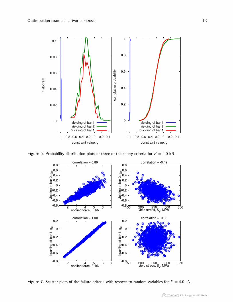
Figure 6. Probability distribution plots of three of the safety criteria for F = 4.0 kN.
-0.8
-0.6
-0.4
-0.2
0
0.2
150 200 250 300 350
bucklin
g o
f bar
1, g
3
yield stress, Sy, MPa
correlation = 0.03
-0.8
-0.6
-0.4
-0.2
0
0.2
1 2 3 4 5 6 7
bucklin
g o
f bar
1, g
3
applied force, F, kN
correlation = 1.00
-0.8
-0.6
-0.4
-0.2
0
0.2
0.4
0.6
0.8
150 200 250 300 350
yie
ldin
g o
f bar
2, g
2
yield stress, Sy, MPa
correlation = -0.42
-0.8
-0.6
-0.4
-0.2
0
0.2
0.4
0.6
0.8
1 2 3 4 5 6 7
yie
ldin
g o
f bar
2, g
2
applied force, F, kN
correlation = 0.89
Figure 7. Scatter plots of the failure criteria with respect to random variables for F = 4.0 kN.
CC BY-NC-ND J.T. Scruggs & H.P. Gavin