Progress In Electromagnetics Research C, Vol. 77, 155–165, 2017

Design of a Microwave Time Reversal Mirror for ImagingApplications

Saptarshi Mukherjee*, Lalita Udpa, Yiming Deng,Premjeet Chahal, and Edward J. Rothwell

Abstract—This paper presents a design of microstrip transmitting and receiving antennas to be usedfor time reversal ultra-wideband imaging applications. The transmitter and receiver arrays are togetherknown as a time reversal mirror (TRM). Based on the properties of time reversal and its imagingapplications, an antipodal Vivaldi antenna and a monopole antenna are proposed for the transmitterand receiver designs, respectively. Simulation and measurement results demonstrate the efficiency of theantennas for a time reversal mirror. The overall system is demonstrated for source and target imagingapplications.

1. INTRODUCTION

Time reversal (TR) is based on the reciprocity property of the wave equation. The time reversed electricand magnetic field components back-propagate to focus at the source location. TR was introduced byMathias Fink in 1992 for ultrasonic imaging and later widely utilized in several ultrasonic applicationssuch as transcranial therapy [1]. It was extended into the realm of electromagnetics by Lerosey et al. [2]and has shown a lot of progress in ultra-wideband (UWB) applications involving radar detection incluttered media [3] and non-destructive evaluation [4]. Research on using microwave TR for imaginghas been limited over the years, but warrants renewed study because of its advantages over conventionalimaging systems. These advantages include its non-iterative nature and its super-resolution and selectivefocusing capabilities [5].

Numerous microstrip antennas have been proposed to cover the UWB frequency band between 3.1and 10.6 GHz released by the Federal Communications Commission for short-range wireless applications.Designing UWB antennas for imaging applications is challenging since unlike narrow-band antennas,UWB antennas must exhibit near-uniform radiation characteristics such as high gain, return losses andlow cross-polarization, over large bandwidths. Moreover, the design of UWB time reversal antennas(TRAs) is particularly challenging, since the antennas need to comply with the unique properties of timereversal. The TRA needs to illuminate most of the region of interest effectively and detect potentialanomalies in presence of other significant scatterers. A lot of different UWB antennas proposed recentlydo not satisfy these requirements. For example, the UWB antenna presented in [7], though having smallsize, lacks both reasonable gain and return losses. Additionally, previous research on microstrip TRAdesigns has proposed using the same transmitting and receiving antenna [8], which is not desirable fortime reversal.

This research proposes a novel design of a time reversal mirror (TRM) for imaging applications.Separate UWB transmitting and receiving antennas operating between 3 to 10 GHz are designed, keepingin consideration the unique features of TR imaging. Comparison between simulation and measurement

Received 18 May 2017, Accepted 21 August 2017, Scheduled 3 September 2017* Corresponding author: Saptarshi Mukherjee (mukher40@egr.msu.edu).The authors are with the Department of Electrical and Computer Engineering, Michigan State University, East Lansing, MI 48824,USA.

156 Mukherjee et al.

results shows good correlation. The proposed TRM has been validated by performing an imagingexperiment using a pulsed time domain laboratory setup, coupled with a back-propagation 2D FDTDcode. Experimental results validate the system’s efficiency and lay the foundation for potential imagingapplications.

2. DESIGN OF AN ANTENNA SYSTEM FOR TIME REVERSAL

The design of the TRA is non-trivial due to several reasons. The contributing factors are as follows(i) Bandwidth. TR is similar to phase conjugation in optics. The range resolution is governed by the

pulse width, with smaller pulse width leading to better detection. A short time-domain pulse hasa half-amplitude bandwidth given by the following relation [9]:

Ω =1πτ

4 ln(2), (1)

where Ω and τ are the bandwidth and pulse width, respectively. Thus, both the transmitting andreceiving antennas should be designed to operate over a wide bandwidth.

(ii) Radiation Pattern. The transmitting antenna needs to have a beam narrow enough to illuminatethe region of interest efficiently with a large gain. However, the beam cannot be too focused, sinceTR theory is based on waves diverging outwards from a point source. In contrast, TR theoryassumes the receiver array to be point receivers [10]. Thus the receiving antennas should behavein radiation mode as point sources having omnidirectional radiation patterns. Since the radiationpattern for the transmitting antenna needs to be different from that of the receiving antenna, thesame antenna cannot be used as both transmitter and receiver.

(iii) Polarization. The confinement of the electric or magnetic field along the plane of propagation leadsto linear polarization. However, antennas may have field components orthogonal to the directionof propagation, leading to cross-polarization. Cross-polarized electric field components from thetransmitting antenna are lost when using a 2D image reconstruction algorithm, thus degrading theoverall imaging quality of the 2-D algorithm [11]. In order to reduce the undesired field components,the cross polarization of the antenna should be maintained as low as possible.Simulation studies for antenna design were performed using the commercial high frequency

electromagnetic field simulation software Ansys HFSS. The antennas were fabricated using conventionalphotolithography. Reflection coefficients were measured using an Agilent N5227A network analyser, andradiation patterns were measured using a SATIMO Starlab near-field measurement system.

3. TRANSMITTING ANTENNA

Based on the crucial factors of the TRA discussed above, a modified slot-edged antipodal Vivaldi(SE APV) antenna is chosen as the transmitting antenna. Introduced by Gibson in 1979 [12], theVivaldi antenna serves as a potential candidate for wide-band applications due to its broad impedancebandwidth and ease of planar structure integration. In conventional Vivaldi antennas, the transitionfrom microstrip to slotline restricts extension of impedance bandwidth and generates high cross-polarization due to asymmetric feeding. With the Vivaldi antenna, the bandwidth limitation due to themicrostrip to slot-line transition can be removed by choosing a proper feed. One solution used in thismanuscript is to use a microstrip to stripline or a two-sided slotline transition [13], as recently used bymany researchers [14, 15]. Thus, no external balun is required to operate with unbalanced transmissionlines that are typically used as microwave feed networks [16].

3.1. Design Parameters

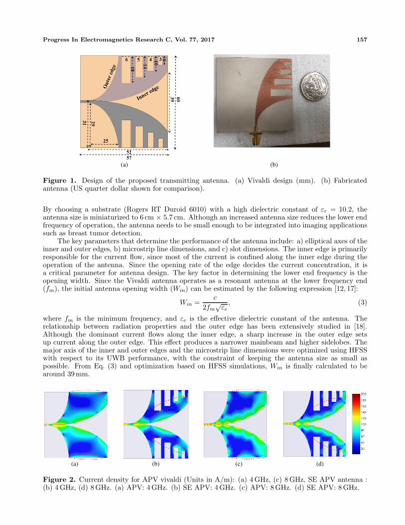
An exploded top-view design of the proposed antenna, along with its dimensions is shown in Fig. 1(a).The fabricated antenna is shown in Fig. 1(b). In this design, the tapered slots are modeled as ellipticaltransitions, with the curve defined as

y = b

√1 − x2

a2, (2)

Progress In Electromagnetics Research C, Vol. 77, 2017 157

(a) (b)

Figure 1. Design of the proposed transmitting antenna. (a) Vivaldi design (mm). (b) Fabricatedantenna (US quarter dollar shown for comparison).

By choosing a substrate (Rogers RT Duroid 6010) with a high dielectric constant of εr = 10.2, theantenna size is miniaturized to 6 cm × 5.7 cm. Although an increased antenna size reduces the lower endfrequency of operation, the antenna needs to be small enough to be integrated into imaging applicationssuch as breast tumor detection.

The key parameters that determine the performance of the antenna include: a) elliptical axes of theinner and outer edges, b) microstrip line dimensions, and c) slot dimensions. The inner edge is primarilyresponsible for the current flow, since most of the current is confined along the inner edge during theoperation of the antenna. Since the opening rate of the edge decides the current concentration, it isa critical parameter for antenna design. The key factor in determining the lower end frequency is theopening width. Since the Vivaldi antenna operates as a resonant antenna at the lower frequency end(fm), the initial antenna opening width (Win) can be estimated by the following expression [12, 17]:

Win =c

2fm√

εe, (3)

where fm is the minimum frequency, and εe is the effective dielectric constant of the antenna. Therelationship between radiation properties and the outer edge has been extensively studied in [18].Although the dominant current flows along the inner edge, a sharp increase in the outer edge setsup current along the outer edge. This effect produces a narrower mainbeam and higher sidelobes. Themajor axis of the inner and outer edges and the microstrip line dimensions were optimized using HFSSwith respect to its UWB performance, with the constraint of keeping the antenna size as small aspossible. From Eq. (3) and optimization based on HFSS simulations, Win is finally calculated to bearound 39 mm.

(a) (b) (c) (d)

Figure 2. Current density for APV vivaldi (Units in A/m): (a) 4 GHz, (c) 8 GHz, SE APV antenna :(b) 4 GHz, (d) 8 GHz. (a) APV: 4 GHz. (b) SE APV: 4GHz. (c) APV: 8 GHz. (d) SE APV: 8 GHz.

158 Mukherjee et al.

3.1.1. SE APV Antenna

The surface current distribution for a conventional APV antenna shows strong edge currents, markedin the dashed-line region A of Figs. 2(a), (c). The currents radiate vertically, leading to undesired sideand back lobes. In order to reduce these surface currents, four slots are etched at the ends of the twinlines of the antenna to form the SE APV antenna. As seen from Figs. 2(b), (d), the modification iscapable of eliminating the unwanted currents at the edges. This leads to an enhanced end fire directionradiation and thus weakens the back-direction radiation.

3.2. Antenna Characteristics in the UWB range

The comparison of simulated and measured reflection coefficients, given in Fig. 3(a), shows goodcorrelation. The slight difference in the measured and simulation results possibly arises due to solderinginaccuracies, introduction of the 50 Ω SMA connector for feeding the antenna or fabrication errors. It isnoted that |S11| ≤ 10 dB over the entire band. Additionally, the impact of a small metallic cylindricaltarget (radius and height 5 mm) in the near-field (1 cm away) of the antenna is observed from Fig. 3(a).The |S11| results show sensitivity due to the presence of the target throughout the frequency band of 3to 10 GHz.

The radiation properties of an antenna vary, depending on the near-field and far-field ranges ofthe antenna. The far-field region is commonly expressed to exist at distances greater than 2D2/λ [17],where D is the maximum dimension of the antenna, and λ is the wavelength. For a UWB antenna, thefar-field distance varies depending on the frequency. For the proposed antenna, the far-field ranges varyapproximately between 0.1 m and 0.5 m. For efficient imaging applications, the sample to be imagedneeds to be in close proximity of the antenna. The antenna may operate in far-field or near-field rangesdepending on the distance between the antenna and the imaging region. Hence the radiation propertiesof the antenna need to be studied for both ranges.

(a) (b)

Figure 3. Transmitting antenna performance. (a) Reflection coefficients comparison. (b) Maximumrealized gain comparison.

3.2.1. Far Field Radiation Patterns

Some of the crucial elements such as gain, radiation pattern and polarization of the antenna canbe determined from the far-field radiation characteristics of the antenna. As shown in Fig. 3(b),the comparison between the simulated and measured boresight gains of the antenna shows slightdiscrepancies; however, the measured realized gain is greater than 5dBi in most of the frequency band.A maximum measured gain of 14 dBi is achieved at 5GHz. The simulated and measured radiationpatterns at 4, 6 and 8GHz (Figs. 4(a), (b), (c)) show good correlation. The antenna shows nice end-fireperformance with the main lobe aligned along the direction of the tapered slots. All the operatingfrequencies maintain the same polarization plane and similar radiation patterns. The transmitting

Progress In Electromagnetics Research C, Vol. 77, 2017 159

antenna has an uniformly narrow beam with a moderately large gain throughout the frequency range.However, the beam is not too focused, which is ideal from the time reversal point of view. As discussedbefore, the cross polarization of the transmitting antenna should be maintained as low as possible. It isnoticed that the cross-polarized gain is much lower than the co-polarized gain throughout the frequencyrange, with a minimum difference at boresight of 8 dBi. The presence of strong horizontal componentsof the surface current radiating electric fields along the sides lead to relatively high cross-polarizationin the E plane.

(a) (c)(b)

Figure 4. Transmitting antenna far field realized gain radiation pattern. (a) E Plane: 4GHz. (b) EPlane: 6 GHz. (c) E Plane: 8 GHz

3.2.2. Near Field Radiation Patterns

The near-field radiation pattern for the transmitting antenna was computed using HFSS at 2 cm radialdistance from the apex of the antenna. Figs. 5(a) and 5(b) present the magnitude of the simulatedradiated electric fields in the E-plane at 4 GHz, 6GHz and 8 GHz. As seen from Fig. 5(a), the E-planeradiation pattern is uniform with the intensities almost equal at all frequencies. The beam is relativelyuniform with a half-power beamwidth (HPBW) of 41.2◦, 32.7◦ and 30◦ at 4GHz, 6 GHz, and 8 GHz,respectively. However, the presence of relatively high intensity side lobes (−4.8 dB for 4 GHz) mightdegrade the imaging quality. Hence, special attention needs to be taken so that the size of the sampleto be imaged is less than or equal to the HPBW of the antenna. Similar radiation intensities noted atall frequencies at θ = 90◦, φ = 90◦ ensure that the peak realized gain is uniform at all frequencies in thenear-field range. The simulated E-field distributions, depicted in Figs. 5(b), (c) for 6 GHz and 10 GHzon xy-plane, show the fields spreading along the tapered slot region and radiating from the top edge ofthe antenna, thus displaying strong end-fire radiation characteristics.

(a) (c)(b)

Figure 5. Transmitting antenna near E-field pattern. (a) E plane near field radiation pattern. (b)Electric field: 6 GHz. (c) Electric field: 10 GHz.

160 Mukherjee et al.

4. RECEIVING ANTENNA

As mentioned before, TR theory assumes the receiver array to be point receivers, along with UWBperformance. Thus, ideally the receiving antennas should have omnidirectional radiation patterns.Conventional monopole antennas have several advantages such as low cost, ease of fabrication andomnidirectional radiation pattern in the transverse plane, but do not yield large bandwidths [17].Recently, several approaches and techniques have been proposed to tailor the antenna towards widebandapplications. In the regime of wideband antennas, planar monopole antennas [7] have garnered hugerecognition due to their flat structure, small size and ease of integration. A planar monopole replaces theconventional wire-element based monopole design with a planar element. In this research, a reduced-ground slotted rectangular (RGSR) monopole is selected as the receiving antenna. The theoreticalresonance frequency (ft) for the fundamental mode of the antenna can be calculated according toEq. (3).

The design starts off with an initial monopole antenna with a reduced ground plane and withoutany feed step. The reduced ground plane is responsible for the wide bandwidth of the antenna, due toabsence of fringing fields between the radiating patch and the ground plane. The length of the groundplane is reduced to λ

10 at the lower frequency end. However, this antenna is matched only at the lowerand higher frequency limits. A double-feed step between the microstrip line and the radiating patchbehaves as quarter wave transformers, thus improving the impedance bandwidth. The blending groundplane edges help in matching at the higher frequencies. The two L-shaped slots (smoothed) in theground plane further help in impedance matching and thus enhance the bandwidth of the antenna andhelp miniaturize it to an area of 3.5 cm by 3.2 cm. Fig. 6 shows the effects of step by step evolution of

(a) (c)(b) (d)

Figure 6. Monopole antenna design and its evolution.

(a) (b)

Figure 7. Receiving antenna. (a) Monopole design (mm). (b) Fabricated monopole antenna.

Progress In Electromagnetics Research C, Vol. 77, 2017 161

(a) (b)

(c) (d)

Figure 8. Proposed receiving antenna and its performance. (a) Reflection coefficients comparison. (b)Radiation pattern: 4 GHz. (c) Radiation pattern: 6 GHz. (d) Radiation pattern: 10 GHz.

Figure 9. Radiation efficiency of the antennas.

Antenna BW ρ (cm) G (dB)SE APV 3.5 6 14

[14] 5.6 6 10[15] 3 8 11.5

RGSR 3.5 3.5 4.2[7] 2.1 3.5 3.6[19] 3.5 4.1 4

Table 1. Comparison of different antennas.

the antenna, as mentioned above. A monopole-like radiation pattern with nulls appearing at the centerfor the E plane omnidirectional radiation in the H plane is observed, with the final evolved design (d),providing the maximum gain.

An exploded top-view design of the RGSR monopole antenna and its dimensions are shown inFig. 7(a). FR4, with a dielectric constant of εr = 4.4, is selected as the substrate since it is inexpensive,thus reducing the cost of fabrication. The fabricated antenna is shown in Fig. 7(b). The comparisonof the simulated and measured reflection coefficients given in Fig. 8(a) show that |S11| < −10 dB overthe entire bandwidth. The simulated and measured E-plane radiation patterns exhibit a monopole-likeradiation as shown in Fig. 8(b). A maximum gain of 4.2 dB is achieved at 6GHz.

An examination of the radiation efficiency of the two antennas shows near constant values across the

162 Mukherjee et al.

specified band of approximately 80–85%, as seen in Fig. 9. A comparison of the performance (fractionalbandwidth (BW), maximum size (ρ) and maximum gain (G)) of the designed antennas with Vivaldiand planar monopole antennas described in the literature is presented in Table 1. It is observed thatthe achieved gain of the SE-APV antenna is much more than that of the antennas presented in [14, 15],while maintaining a small size and comparable BW. Similarly, the RGSR antenna achieves higher gainand BW than the UWB antennas proposed in [7, 19], while maintaining a comparable size. Besides theimproved antenna performance, the concept of using different transmitter and receiver antennas, as wellas choosing specific antenna types in order to implement TR for imaging applications, is introducedin this research. Using different antennas is greatly desirable due to several factors as mentioned inSection 2.

5. TIME DOMAIN CHARACTERIZATION

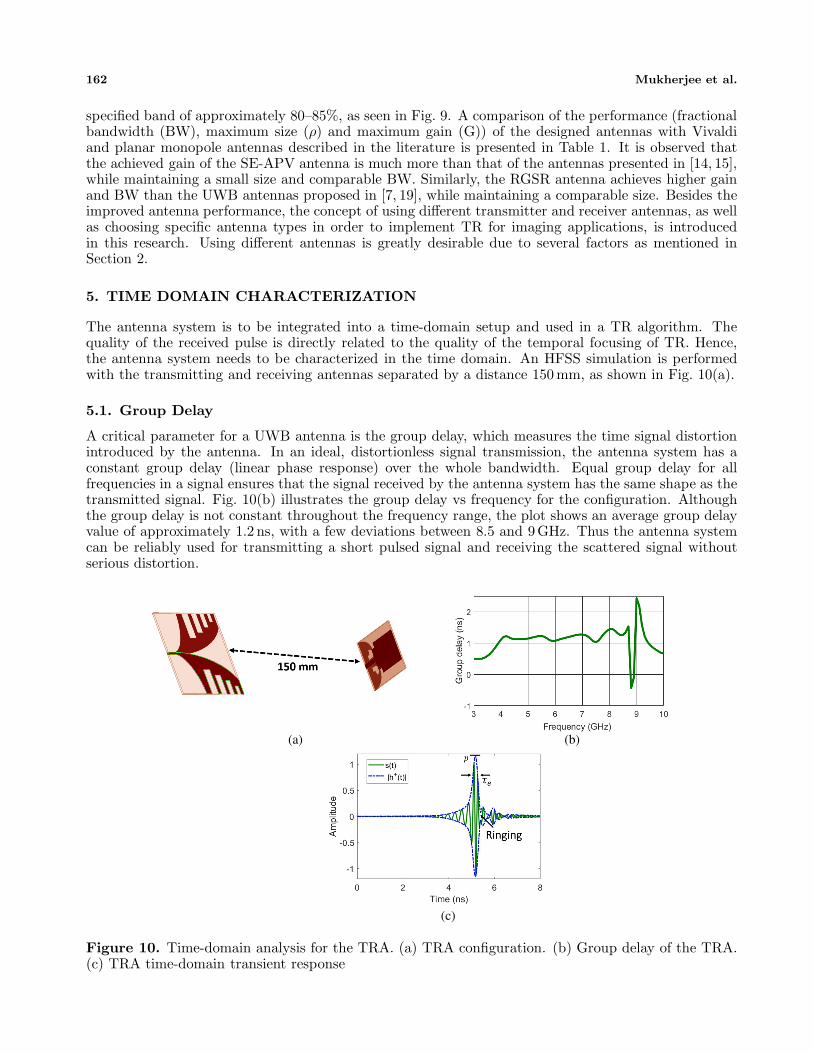
The antenna system is to be integrated into a time-domain setup and used in a TR algorithm. Thequality of the received pulse is directly related to the quality of the temporal focusing of TR. Hence,the antenna system needs to be characterized in the time domain. An HFSS simulation is performedwith the transmitting and receiving antennas separated by a distance 150 mm, as shown in Fig. 10(a).

5.1. Group Delay

A critical parameter for a UWB antenna is the group delay, which measures the time signal distortionintroduced by the antenna. In an ideal, distortionless signal transmission, the antenna system has aconstant group delay (linear phase response) over the whole bandwidth. Equal group delay for allfrequencies in a signal ensures that the signal received by the antenna system has the same shape as thetransmitted signal. Fig. 10(b) illustrates the group delay vs frequency for the configuration. Althoughthe group delay is not constant throughout the frequency range, the plot shows an average group delayvalue of approximately 1.2 ns, with a few deviations between 8.5 and 9GHz. Thus the antenna systemcan be reliably used for transmitting a short pulsed signal and receiving the scattered signal withoutserious distortion.

(b)(a)

(c)

Figure 10. Time-domain analysis for the TRA. (a) TRA configuration. (b) Group delay of the TRA.(c) TRA time-domain transient response

Progress In Electromagnetics Research C, Vol. 77, 2017 163

5.2. Time Domain Response

The transient response for the specific configuration shown in Fig. 10(a) is also studied. The receivedsignal s(t) can be represented by a convolution of the impulse response, as given by the followingexpression [6]:

s(t) = uTx(t) ∗ hTx(t, θ, φ) ∗ hch(t) ∗ hRx(t, θ, φ). (4)

Here uTx is the transmitted signal, and hTx, hch and hRx are the transmitting antenna, medium channeland receiving antenna impulse response functions, respectively. For the schematic shown in Fig. 10(a),the complex S21 measurements are transformed into the time domain to obtain the received time pulse.The received time signal is shown in Fig. 10(c). The antenna dispersion can be analyzed from itsanalytic impulse response, which is calculated by the Hilbert transform H of s(t), given by h+(t) [6].The envelope |h+(t)| localizes the energy distribution versus time and thus measures the dispersion ofan antenna. The specific quantities investigated in this case are:

• Peak Value of envelope p(θ, φ). This quantity is a measure of the maximum value of the strongestpeak of the time domain response. A high peak value is desirable, since it ensures a stronger peak.As seen from Fig. 10(c), a value of p(θ, φ) of 1.16 is achieved.

• Envelope width τe. The envelope width is a measure of the temporal broadening of the radiatedimpulse. Practically, τe should be small in order to obtain high resolution and data rate. The rangeresolution is governed by τe, with smaller pulse width leading to better resolution. The envelopewidth can be obtained from the full width at half maxima of the envelope. As seen from Fig. 10(c),a τe value of 160 ps is achieved.

• Ringing. Several factors such as multiple reflections in the antenna are responsible for oscillationsof the received pulse after the main peak, as observed from Fig. 10(c). This phenomenon is knownas ringing. Ideally, the duration of ringing (τr) should be less than a few τe. Specifically, a highvalue of τr is undesirable for temporal focusing of the time reversed electromagnetic fields. Thetime duration within which the envelope has fallen from p(θ, φ) to a lower bound α · p(θ, φ) ismeasured as τr. As seen from Fig. 10(c), a value of τr for α = 0.1 of 200 ps is achieved.

6. EXPERIMENTAL RESULTS

A passive TR experiment for imaging a metallic cylinder (radius 1.6 cm) was conducted using a pulsedtime domain laboratory setup and a FDTD 2D code for back-propagation of the TR fields [20]. Theexperimental configuration and setup are shown in Figs. 11(a) and 11(b) and explained in details in [20].A small arch range of radius 10 cm with a circular platform was used to position the antennas. Thereceiving monopole antenna was moved, while keeping the transmitting Vivaldi antenna stationary, inorder to emulate the receiver array system. The time domain system generates a pseudo-Gaussian pulsesignal of bandwidth 10 GHz, which is fed as input to the Vivaldi antenna.

The setup is a miniaturized version of [20], tailored for precise near field imaging applications, suchas micro-cracking detection in composite NDE and breast tumor diagnosis in medical imaging. Whilethe experiments in [20] are meant for far-field detection purposes only, the present setup can work bothin transmission and reflection modes (with 350 degrees coverage) as a near-field and far-field system,in order to gain better imaging quality. Since all parts of the setup, including the sample stand andantenna stands, can be adjusted, it is possible to measure cross-polarized field components and thusthe potential for performing 3D imaging. Moreover, while horn antennas were used in [20] for targetlocalization experiments in the reflectivity arch-range, they could not be utilized for near-field imagingin the mini-arch range setup, since they produce a plane wave at far-field distances (∼ 3.5 m) and areintended for diffraction limited imaging. Additionally, the relatively large size and 3D structure of thehorn antennas make them undesirable for compact imaging applications due to inefficient illumination ofthe imaging domain, size and weight constraints and their inability to be integrated into planar circuits.Hence the designed planar microstrip antennas are preferred candidates for the mini arch-range setupshown in Fig. 11(a).

The scattered fields from the target are recorded by the monopole antenna. These fields are timereversed and back-propagated using the numerical model. At the localized time instant, the electric

164 Mukherjee et al.

(a) (b)

Figure 11. (a) Time domain scattering measurement configuration. (b) Experimental setup.

(a) (b) (c) (d)

Figure 12. Target imaging experiment: (a) Electric fields focused at metal rod. (b) Simulated energyimage. (b) Experimental energy image. (d) Cross-range signal comparison.

fields are efficiently focused at the metal target location, as displayed in Fig. 12(a). The time integratedelectric energy shows the energy localized around the target region, as displayed in Fig. 12(c). The fullwidth at half maximum (1.8 cm) of the cross range energy signal, indicated by the solid black line ofFig. 12(d) can be utilized to estimate the actual size of the target. A simulation is performed for thesimilar configuration using 2D FDTD codes, demonstrating excellent comparison between experimentaland simulated results, as shown in Figs. 12(b), (c) and (d)).

7. CONCLUSION

Microstrip transmitting and receiving antennas, operating between 3 GHz and 10 GHz, are designed tobe used in a TRM for imaging applications. A TSE APV antenna and an RGSR monopole antennaare proposed and developed as the transmitting and receiving antennas of the system. The efficacy ofthe transmitting antenna was evaluated at both far- and near-field ranges. The antennas are optimizedaccording to the requirements of the system, characterized in both frequency and time domain, andfabricated. There is good match between simulation and measurement results. Measurement resultsshow that both antennas meet the requirements for a TR system. Accurate measurement resultsdemonstrate the feasibility of the TRA for imaging applications. The imaging system can be usedin several applications such as complicated long range radar imaging, rapid inspection of compositesand breast tissue imaging. Future work involves evaluating the super-resolution capabilities of TR andtesting the robustness of the system for detection of tumors in realistic multi-layered breast phantomsas well as nondestructive evaluation of composite structures.

Progress In Electromagnetics Research C, Vol. 77, 2017 165

REFERENCES

1. Thomas, J.-L. and M. A. Fink, “Ultrasonic beam focusing through tissue inhomogeneities with atime reversal mirror: application to transskull therapy,” IEEE Trans. Ultrason., Ferroelect., Freq.Control, Vol. 43, No. 6, 1122–1129, Nov. 1996.

2. Lerosey, G., J. De Rosny, A. Tourin, A. Derode, G. Montaldo, and M. Fink, “Time reversal ofelectromagnetic waves,” Phys. Rev. Lett., Vol. 92, No. 19, 193904, 2004.

3. Zhang, W., A. Hoorfar, and L. Li, “Through-the-wall target localization with time reversal musicmethod,” Progress In Electromagnetics Research, Vol. 106, 75–89, 2010.

4. Rodrıguez, S., N. Lei, B. Crowgey, L. Udpa, and S. S. Udpa, “Time reversal and microwavetechniques for solving inverse problem in non-destructive evaluation,” NDT & E Intl., Vol. 62,106–114, 2014.

5. Devaney, A. J., E. A. Marengo, and F. K. Gruber, “Time-reversal-based imaging and inversescattering of multiply scattering point targets,” J. Acoust. Soc. Am., Vol. 118, No. 5, 3129–3138,2005.

6. Wiesbeck, W., G. Adamiuk, and C. Sturm, “Basic properties and design principles of UWBantennas,” Proceedings of the IEEE, Vol. 97, No. 2, 372–385, 2009.

7. Lim, K.-S., M. Nagalingam, and C.-P. Tan, “Design and construction of microstrip UWB antennawith time domain analysis,” Progress In Electromagnetics Research M, Vol. 3, 153–164, 2008.

8. Nadia Maaref, P. M., X. Ferrieres, C. Pichot, and O. Picon, “Electromagnetic imaging methodbased on time reversal processing applied to through-the-wall target localization,” Progress InElectromagnetics Research M, Vol. 1, 59–67, 2008.

9. Crowgey, B. R., E. J. Rothwell, L. C. Kempel, and E. L. Mokole, “Comparison of UWB short-pulseand stepped-frequency radar systems for imaging through barriers,” Progress In ElectromagneticsResearch, Vol. 110, 403–419, 2010.

10. Fink, M., “Time reversal of ultrasonic fields. i. basic principles,” IEEE Trans. Ultrason., Ferroelect.,Freq. Control, Vol. 39, No. 5, 555–566, 1992.

11. Kosmas, P. and C. M. Rappaport, “FDTD-based time reversal for microwave breast cancerdetection-localization in three dimensions,” IEEE Transactions on Microwave Theory andTechniques, Vol. 54, No. 4, 1921–1927, 2006.

12. Gibson, P. J., “The Vivaldi aerial,” 9th European Microwave Conference, 101–105, IEEE, 1979.13. Gazit, E., “Improved design of the Vivaldi antenna,” IEE Proceedings H (Microwaves, Antennas

and Propagation), Vol. 135, 89–92, IET, 1988.14. Kota, K. and L. Shafai, “Gain and radiation pattern enhancement of balanced antipodal Vivaldi

antenna,” Electronics Letters, Vol. 47, No. 5, 303–304, 2011.15. Wang, P., H. Zhang, G. Wen, and Y. Sun, “Design of modified 6–18 GHz balanced antipodal Vivaldi

antenna,” Progress In Electromagnetics Research C, Vol. 25, 271–285, 2012.16. Balanis, C. A., Modern Antenna Handbook, John Wiley & Sons, 2011.17. Balanis, C. A., Antenna Theory: Analysis and Design, John Wiley & Sons, 2016.18. Greenberg, M. C., K. L. Virga, and C. L. Hammond, “Performance characteristics of the

dual exponentially tapered slot antenna (detsa) for wireless communications applications,” IEEETransactions on Vehicular Technology, Vol. 52, No. 2, 305–312, 2003.

19. Abbosh, A. M. and M. E. Bialkowski, “Design of ultrawideband planar monopole antennas ofcircular and elliptical shape,” IEEE Transactions on Antennas and Propagation, Vol. 56, No. 1,17–23, 2008.

20. Mukherjee, S., L. Udpa, S. Udpa, and E. Rothwell, “Target localization using microwave timereversal mirror in reflection mode,” IEEE Transactions on Antennas and Propagation, Vol. 65,No. 2, 820–828, 2016.