Design of a Helicopter Slung Vehicle for Actuated Payload ...
118
Design of a Helicopter Slung Vehicle for Actuated Payload Placement Robert James Collins Thesis submitted to the faculty of the Virginia Polytechnic Institute and State University in partial fulfillment of the requirements for the degree of Master of Science In Mechanical Engineering Kevin B. Kochersberger, Chair Christopher B. Williams Alexander Leonessa April 12, 2012 Blacksburg, Virginia Keywords: Tethered Payload, Helicopter, Slung Load, Autonomous Systems Copyright 2012, Robert J. Collins
Transcript of Design of a Helicopter Slung Vehicle for Actuated Payload ...

Design of a Helicopter Slung Vehicle for Actuated Payload Placement
Robert James Collins
Thesis submitted to the faculty of the
Virginia Polytechnic Institute and State University
in partial fulfillment of the requirements for the degree of
Master of Science
In
Mechanical Engineering
Kevin B. Kochersberger, Chair
Christopher B. Williams
Alexander Leonessa
April 12, 2012
Blacksburg, Virginia
Keywords: Tethered Payload, Helicopter, Slung Load, Autonomous Systems
Copyright 2012, Robert J. Collins

Design of a Helicopter Slung Vehicle for Actuated Payload Placement
Robert James Collins
Abstract
Helicopters have been used in applications where they need to carry a slung load for
years. More recently, unmanned (UAV) helicopters are being used to deliver supplies to military
units on the ground in theaters of war. This thesis presents a helicopter slung vehicle used to
carry the payload and furthermore, provide a means of actuation for the payload. This provides
more control authority to the system and may ultimately allow a helicopter to fly higher with a
longer tether.
The vehicle designed in this thesis was designed for use with 100kg class helicopters,
such as the Yamaha RMAX operated by the Virginia Tech Unmanned Systems Lab. Each
system on the vehicle was custom designed – including the propulsion system, wall detection /
localization system, and controller. Three shrouded propellers provided thruster actuation. A
scanning laser range finder and inertial measurement unit (IMU) were used to provide
localization. A first attempt at a linear full state feedback controller with a complementary filter
was used to control the vehicle.
All of the systems were tested individually for functionality. The shrouded propellers met
their design goals and were capable of producing .7lbf of thrust each. The wall detection system
was able to detect walls and windows reliably and with repeatability. Results from the controller
however were less than ideal, as it was only able to control yaw in an oscillatory motion, most
likely due to model deficiencies. A reaction wheel was used to control yaw of the vehicle with
more success.

iii
Acknowledgements
I’d like to first acknowledge and thank my advisor, Dr. Kevin Kochersberger, for
allowing me to work in the lab and furthermore, allowing me to work on this project. In addition,
I would like to thank the other members of my committee for their assistance.
I’d also like to thank those whom I’ve worked with over the past year in the Unmanned
Systems Lab. Starting off; I’d like to thank Ken Kroeger, for providing assistance whenever
possible, including his time in the machining of some of the components that made up this
assembly. In addition, I’d like to thank Bryan Krawiec and Pete Fanto for their insight as well.
Those others who also worked in the USL need to be acknowledged, for they also provided at the
very least an occasional distraction, which was critical in the interest of my sanity.
Finally, I’d like to thank my family and my parents for their encouragement and support.
They encouraged me to work hard and to continue my education.
All photos by the author, 2012.

iv
Table of Contents
1. Introduction ............................................................................................................................... 1
1.1 Project Motivation ................................................................................................................ 2
1.1.1 Design Requirements ..................................................................................................... 3
1.2 Overview of Thesis ............................................................................................................... 3
2. Literature Review ..................................................................................................................... 5
2.1 Current Supply Techniques................................................................................................... 5
2.2 Control of Tethered Systems ................................................................................................ 6
2.3 Propulsion System ................................................................................................................ 8
2.4 Line Detection ....................................................................................................................... 9
3. Propulsion System Design ...................................................................................................... 11
3.1 Propulsion System Requirements ....................................................................................... 11
3.2 Selecting a Propulsion Method ........................................................................................... 12
3.2.1 Power Generation and Delivery .................................................................................. 12
3.2.2 Addressing Power Consumption .................................................................................. 13
3.3 Shrouded Propeller Design ................................................................................................. 17
3.3.1 Shrouded Propeller Requirements ............................................................................... 17
3.3.2 Initial Shrouded Propeller Design ............................................................................... 19
3.3.3 Initial Shrouded Propeller Testing .............................................................................. 25
3.3.4 Final Shrouded Propeller Design ................................................................................ 28
3.4 Final Shrouded Propeller Testing ....................................................................................... 30
4. Wall Detection ......................................................................................................................... 33
4.1 System Requirements.......................................................................................................... 33
4.2 Wall Detection Algorithm ................................................................................................... 34
4.2.1 The Hough Transform .................................................................................................. 34
4.2.2 Wall Detection Algorithm Pseudo-Code ...................................................................... 36
4.2.3 Wall Detection Testing ................................................................................................. 37
4.3 Window Detection Algorithm ............................................................................................. 39
4.3.1 Window Detection Algorithm and Pseudo-Code ......................................................... 40
4.3.2 Window Detection Testing ........................................................................................... 40
5. Tethered Supply Vehicle Design ............................................................................................ 42
5.1 Vehicle Requirements ......................................................................................................... 42
5.2 Vehicle Electronics and System Architecture ..................................................................... 44

v
5.2.1 Navigational System..................................................................................................... 44
5.2.2 Vehicle Onboard Computer ......................................................................................... 44
5.2.3 Propulsion System Electronics .................................................................................... 45
5.2.4 Wireless Communication ............................................................................................. 46
5.2.5 System Architecture Overview ..................................................................................... 46
5.3 Design and Implementation of Software User Interface ..................................................... 48
5.4 Dynamic System Modeling................................................................................................. 49
5.4.1 Equations of Motion ..................................................................................................... 50
5.4.2. Thruster Placement for Controllability ...................................................................... 51
5.5 Vehicle Mechanical Design ................................................................................................ 54
5.5.1 Designing for Requirements ........................................................................................ 54
5.5.2 Sensor and Electronics Placement............................................................................... 55
5.5.3 Structural Considerations ............................................................................................ 56
5.6. Vehicle Fabrication ............................................................................................................ 60
6. Controller Design and Implementation ................................................................................ 62
6.1 Spherical Pendulum Dynamics ........................................................................................... 62
6.2 Collecting Data and Filtering .............................................................................................. 64
6.2.1 Data Collection ............................................................................................................ 64
6.2.2 Sensor Filtering ........................................................................................................... 65
6.3 Controller Design ................................................................................................................ 69
6.3.1 Multiple Input Multiple Output Control ...................................................................... 69
6.3.2 Modeling Deficiencies ................................................................................................. 73
6.4 Controller Implementation .................................................................................................. 74
6.4.1 Verifying the Controller ............................................................................................... 74
6.5 Momentum Actuation and Control ..................................................................................... 77
6.5.1 Reaction Wheel Design ................................................................................................ 78
6.5.2 Reaction Wheel Dynamic Model .................................................................................. 79
6.5.3 Controller Implementation........................................................................................... 80
7. Conclusion and Recommendations ....................................................................................... 84
7.1 Summary of Work............................................................................................................... 84
7.2 Suggestions for Future Work .............................................................................................. 86
Bibliography ................................................................................................................................ 88
Appendices ................................................................................................................................... 90
Appendix A - Shrouded Propeller Static Thrust Theory ........................................................ 91

vi
Appendix B - Derivation of Spherical Pendulum Equations of Motion ................................ 93
Appendix C - Mechanical Prints ............................................................................................... 95

vii
List of Figures
1.1. A slung payload with an actuated payload vehicle. ................................................................. 1
2.1. A ground robot being deployed from the VT Unmanned System Lab Yamaha R-MAX. ...... 6
3.1. The Hacker A20-30M brushless motor.................................................................................. 13
3.2. Flow field illustrated for the shrouded and free propeller cases. ........................................... 14
3.3. Theoretical thrust ratio for a given area ratio......................................................................... 15
3.4. A plot of static thrust versus power required for an area ratio of 1.00 and 1.29. .................. 16
3.5. A plot of separation on a NACA 4416 airfoil. ....................................................................... 19
3.6. The influence of area ratio on static thrust output. ................................................................ 20
3.7. A generic shroud with a toroid lip design. ............................................................................. 22
3.8. The first prototype shroud design. ......................................................................................... 23
3.9. The first prototype shroud design as a solid model. .............................................................. 24
3.10. The first prototype shroud design being printed on a FDM rapid prototyping machine ..... 25
3.11. Flow visualization - the flow appears attached throughout the shroud ............................... 26
3.12. Separated flow field at the lip and diffuser .......................................................................... 26
3.13. Static thrust as a function of power and rotational speed of the propeller. .......................... 27
3.14. Figure of merit plotted as a function of rotational speed of the propeller. .......................... 28
3.15. Revised shroud design, showing manufacturing and assembly methods. ........................... 29
3.16. Shroud center assembly fixture, used to place the components in their proper plane and to
ensure that they were concentric. .................................................................................................. 30
3.17. Three assembled shrouds used on the final assembly of the vehicle. .................................. 30
3.18. Static thrust as a function of power and rotational speed of the propeller ........................... 31
3.19. Static thrust as a function of PWM duty cycle in microseconds ......................................... 32
4.1. Sample output from the URG-04LX...................................................................................... 34
4.2. A sample data set having a slope of -1 and a y-intercept of 1. .............................................. 35
4.3. The Hough space of the sample data set presented in Figure 4.2. ......................................... 36
4.4. Sample record of distance and angle, calculated by the wall detection algorithm ................ 38
4.5. Sample record of detected window width .............................................................................. 41
5.1. A picture of the MicoStrain 3DM-GX2 IMU. ....................................................................... 44
5.2. A picture of the ADLS15PC PC104. ..................................................................................... 45
5.3. A picture of the Arduino MEGA. .......................................................................................... 46
5.4. Block diagram of the system architecture. ............................................................................. 47
5.5. Screenshot of the user interface for the tethered supply vehicle. .......................................... 49
5.6. Diagram showing the generalized coordinates of the thrusters. ............................................ 50

viii
5.7. Diagram showing 2D pendulum motion. ............................................................................... 51
5.8. Original Simulink model used to design the vehicle for controllability. ............................... 52
5.9. Simulated thruster output for a 10 degree yaw initial condition. ........................................... 54
5.10. Yamaha RMAX landing gear with the USL developed winch pod attached. The tethered
vehicle was designed to fit in the underside volume. ................................................................... 55
5.11. Solid model of the tethered vehicle’s base structure ........................................................... 56
5.12. The bottom of the vehicle is illustrated here to show the designed supporting structure. ... 57
5.13. A plot of the averaged von mises stress on the loaded vehicle. ........................................... 59
5.14. Left – the individual components of the vehicle structure are shown before assembly. Right
– vehicle is in the process of being riveted. .................................................................................. 60
5.15. The vehicle with all of the subsystems installed. ................................................................. 61
6.1. A generic model of a spherical pendulum attached to a fixed point. ..................................... 62
6.2. Yaw and velocity measurements, unfiltered and not complemented with any other data
source. ........................................................................................................................................... 66
6.3. Block diagram of the complementary filter. .......................................................................... 67
6.4. The perpendicular angle from the wall filtered and unfiltered. ............................................. 68
6.5. The perpendicular distance filtered and unfiltered. ............................................................... 69
6.6. Original Simulink model used to design the full state feedback controller. .......................... 71
6.7. The continuous and discrete responses. ................................................................................. 72
6.8. Simulated actuator / thruster output for the continuous and discrete implementations of the
controller. ...................................................................................................................................... 73
6.9. Comparison of actual yaw data to simulated data. ................................................................ 75
6.10. Comparison of actual yaw data to corrected simulated data. ............................................... 77
6.11. The reaction wheel system layout. ....................................................................................... 78
6.12. The reaction wheel implemented onboard the vehicle. ....................................................... 79
6.13. Yaw performance using the reaction wheel at steady state. ................................................ 81
6.14. Yaw performance using the reaction wheel with an initial condition of approximately 15
degrees. ......................................................................................................................................... 82
A-1. Cross section of a generic shrouded propeller. ..................................................................... 91
B-1. A generic model of a spherical pendulum attached to a fixed point. .................................... 93

ix
List of Tables
3.1. A morphological matrix used to design the shroud. .............................................................. 21
3.2. Concept selection matrix of lip choices. ................................................................................ 23
4.1. Wall finding algorithm runtimes. ........................................................................................... 39
5.1. Thruster placement parameters .............................................................................................. 53
5.2. Material properties used in the linear static deformation finite element model. ................... 58
5.3. Stresses and deflections as calculated from the finite element model. .................................. 59
6.1. Instrument Update Rates for the primary instruments used onboard the vehicle. ................. 64
6.2. Instrument used for each dynamic state measurement. ......................................................... 65
6.3. Physical parameters used in designing the linear full state feedback controller. ................... 73
6.4. Physical parameters of the reaction wheel. ............................................................................ 79

x
List of Symbols
The following symbols were used for shrouded propellers:
T static thrust
A area
ρ density of air
P power
M factor of merit
D diameter
The following subscripts were used for shrouded propellers:
s shrouded propeller
f free propeller
e exit
p propeller disc
The following symbols were used for wall detection:
R distance
x Cartesian x coordinate
y Cartesian y coordinate
θ angle of wall
The following subscripts were used for wall detection:
i ith
point, counter
The following symbols were used for the mechanical design:
M moment
x position along beam
ω loading per length

xi
δ deflection
σ normal stress
c distance from neutral axis
E modulus of elasticity
I area moment of inertia
l length of beam
The following symbols were used for spherical pendulum dynamics:
θ pendulum angle
φ precession angle
The following symbols were used for linear control dynamics:
J vehicle moment of inertia
I reaction wheel moment of inertia
θ yaw angle
R thruster moment arm
T thrust
c linear damping coefficient
m mass
x position from wall
φ angle of thrusters
g gravitational constant
L tether length
e bias error
t time
b bias
τ filter time constant

xii
s Laplace variable
K gain matrix
A impulse amplitude
ζ damping ratio
T vibration period
ω frequency, rad/s
The following subscripts were used for linear control dynamics:
1 station 1
2 station 2
3 station 3
4 station 4
i ith
impulse, counter
w reaction wheel

Robert J. Collins Introduction 1
Chapter 1 Introduction
This thesis presents the design of a helicopter slung vehicle actuated by three thrusters for
payload placement control, with the ultimate goal of increasing the slung-load system’s total
control authority and stability. The vehicle will be used for the actuated placement of payloads
from a mid-sized 100kg class unmanned helicopter. This can be useful in applications where a
tethered payload needs to navigate a small area and / or an area that may consist of obstacles
such as buildings or irreplaceable property. A hypothetical system consisting of an actuated
slung vehicle is shown in Figure 1.1.
Figure 1.1. A slung payload with an actuated payload vehicle. The actuated payload vehicle provides
more control authority to the slung-load system.
Helicopters and fixed wing aircraft are regularly used to deliver equipment and supplies
quickly and effectively. Aircraft are used in this capacity routinely with the armed forces,
commercial operations, and for humanitarian aid. Helicopters in particular are used routinely in
conjunction with slung / tethered payloads. Such examples include aerial cranes, firefighting, and
military operations. However, such operations can be unsafe for not only people and property on

Robert J. Collins Introduction 2
the ground, but also for the pilot / crew and the payload itself. This thesis presents a tethered
vehicle with thrusters, a navigation system, and a controller that can be used to place payloads on
the ground and avoid obstacles (such as walls), as shown previously in Figure 1.1. In normal
tethered payload operations, the helicopter is used to position the payload. This thesis presents a
vehicle capable of carrying a 5kg payload of which can actuate and position itself.
Each of the different subsystems used in the vehicle – propulsion, wall detection, and the
controller had to be designed. Software to debug and control the vehicle was written for the
onboard computer and microcontroller. The vehicle was fabricated as a 16”x16” planform area,
weighing 8.1lb empty. After fabrication, the vehicle was tethered to a fixed point at the
Unmanned Systems Lab to begin testing it. This thesis presents the design, research, fabrication,
and testing of the tethered vehicle.
1.1 Project Motivation
Payloads are currently slung / tethered from helicopters using relatively short tethers
lengths. This allows the helicopter to provide position control of the payload. However,
situations may arise where the payload needs to be navigated and placed near buildings, people,
or other areas where property damage and harm could occur. In these situations, control authority
of the helicopter may not be enough, especially if disturbances such as wind, gusts, rotor
downwash, etc impact the payload. Depending on the amplitude of the sway, the helicopter itself
may become uncontrollable.
In addition, long tether operations may be of interest. Using a long tether, helicopters can
fly at a higher altitude. In a military application, this would permit a helicopter to fly out of
acoustic range and to avoid small arms fire. Controlling a tethered payload with a long tether can
present issues due to the disturbances and large accelerations that the helicopter must undergo to
cancel out the sway. It is likely that the helicopter will not have enough control authority for a
payload slung by a long tether, thus an actuated vehicle will likely need to be used for control.
While long tether operations were not a focus of this particular thesis, the vehicle developed in
this thesis could potentially be used in long tether operations utilizing the proper control
techniques.
Even though the dynamics derived in this thesis only account for short tether operations,
a practical implementation of the vehicle is still novel and useful. Unmanned helicopters have

Robert J. Collins Introduction 3
only recently been used to carry tethered payloads. Utilizing a vehicle with thruster actuators to
carry the payload can help with positioning and the overall control of the system, providing a
factor of safety.
1.1.1 Design Requirements
Considering the overall motivation of the project, several broad design requirements of
the vehicle can be derived. These include:
The vehicle must be able to locate obstacles and position itself. This is the crux
of the problem. In order to position itself without the aid of the helicopter, the
vehicle needs to have onboard thrusters. Localization of obstacles such as walls is
necessary for the controller to actuate the thrusters.
The vehicle must be able to localize itself using onboard sensors. It is necessary
to develop a vehicle that can localize and control itself / the payload using only
the information gathered by onboard sensors and without the aid of GPS. This
eliminates the need to communicate to the helicopter for orientation information
and provides reliable measurements of the dynamic states. The vehicle will need
to be completely self-powered.
The vehicle must weigh less than 5kg empty and must be able to carry a payload
of 5kg. This requirement is derived from the typical maximum payload of the
100kg class helicopter (10kg). The tethered vehicle developed in this thesis was
designed to be tethered with the Virginia Tech Unmanned Systems Lab’s RMAX
helicopter.
1.2 Overview of Thesis
This thesis first presents the previous work done in the field of tethered operations and
payload control. In particular, this includes research on sway control of cranes and control
techniques such as input shaping. Since the vehicle encompasses multiple, very different
systems, the theory used to design each individual system (propulsion, wall detection, etc) is
presented as well.
The design and performance of each system is then discussed. The propulsion system is
first presented. Starting off with the design requirements, the fundamental theory and prior

Robert J. Collins Introduction 4
research conducted on shrouded propellers is discussed in more detail. A design which results in
a 5” inner diameter shroud results and is presented along with relevant (static thrust) test data and
characterization curves.
Next, the wall and window detection algorithm are discussed. A theoretical overview of
the Hough transform as a line detection technique (used to detect walls, which would likely be an
obstacle to avoid while the vehicle is deployed) is given. The actual implementation using a
scanning laser range finder and a custom written LabVIEW program is then presented.
Performance is shown in terms of computational speed and measurement repeatability.
The next chapter presents the system architecture and mechanical design of the overall
tethered vehicle. The electrical hardware is selected, including the inertial measurement unit, the
laser range finder, and the onboard computer / wireless communication hardware. Basic control
theory is then discussed as it was used to ensure the vehicle would remain controllable. The
resultant mechanical design is then presented.
System dynamics and the controller are then discussed. The linearized equations of
motion are presented along with the accompanying linear control law used. The vehicle
controller is coded, implemented, and tested in this chapter.
Finally, the thesis concludes with a summary of work and suggestions for future work /
improvements. Several deficiencies presented themselves, mostly during the implementation of
the controller. These deficiencies are discussed with suggestions on how to minimize them.

Robert J. Collins Literature Review 5
Chapter 2 Literature Review
Designing a helicopter tethered vehicle for supplying ground units requires many sub-
systems. In particular, such a vehicle would need a vision system to detect obstacles for the
ultimate goal of locating and avoiding them. Once an obstacle is located, a propulsion system is
necessary to ensure the vehicle does not collide with the obstacle. Finally, in order to control the
vehicle in a meaningful manner, a controller would need to be implemented. This chapter
discusses an overview of each of these systems that were used in the design and fabrication of
the resupply vehicle.
2.1 Current Supply Techniques
Airborne supply missions have been and will continue to be a critical component of
modern logistics. Aircraft have been delivering supplies in a commercial, humanitarian, and
military capacity for almost as long as airplanes have been around. In World War II,
accompanying the development of airborne paratrooper units, military units began to airdrop
supplies to ground units by strapping parachutes to cargo. Airdrop techniques evolved as loads
and requirements changed. Various methods exist for extracting loads out of airplanes and to
slow the rate of decent of the airdropped cargo [1]. Different aircraft have evolved and are used
for different missions and load carrying capability. Today, the United States Air Force’s C-5
Galaxy is able to air drop 200,000 pounds of material utilizing multiple pallets [1].
Airdrops are effective at distributing large amounts of cargo. However, they’re not the
only technique used to deliver supplies in the military’s supply chain. If there is a large enough
airstrip in the destination area, cargo aircraft can land to deliver supplies. Vehicle convoys are
often used to deliver supplies and transport people. Helicopters are used frequently as well,
especially in areas that have little to no supporting infrastructure (roads, bridges, runways) and
may be home to dangerous terrain.
Helicopters are often used to transport large loads, often larger than the helicopter is
itself. This requires the load to be tethered to the helicopter. Tethering a load to a helicopter is
not entirely new. This is a common practice with helicopters used in aerial firefighting and as
aerial cranes. The Unmanned Systems Lab at Virginia Tech routinely executes tethered payload

Robert J. Collins Literature Review 6
operations from a Yamaha RMAX, mostly utilizing it to deploy a ground based tracked robot.
This is shown in Figure 2.1.
Figure 2.1. A ground robot being deployed from the VT Unmanned System Lab Yamaha R-MAX.
In December 2011, autonomous K-MAX helicopters developed by Lockheed Martin and
Kaman went into service for the sole purpose of transporting supplies. The Navy’s major
motivation for developing this project was to avoid the hazards of ground based supply convoys,
as they are easily targetable by makeshift explosives. Operating since December 17, 2011, the
helicopters have been successful at delivering more than 100,000lbs as of January 31, 2012 [2].
2.2 Control of Tethered Systems
Tethered systems such as a tethered payload attached to a helicopter or to a crane are
often times uncontrolled. Depending on the mechanics of the system, this may or may not be
acceptable. For example, if a long tethered payload is attached to a crane, a disturbance or even
the stoppage of the crane could cause the payload to sway. This could be dangerous to property
or people in the surrounding area. Sway can also influence the system’s speed and accuracy.
To address the problem of sway, engineers have most notably used a technique called
input shaping. Input shaping is a feed-forward control technique, not requiring any

Robert J. Collins Literature Review 7
instrumentation for feedback. Rather, the input shaper only requires knowledge of the natural
frequency of the system. By utilizing the natural frequency of the system, the input shaper
manipulates the user’s desired commands to effectively cancel out the system sway [3].
This technique has been used with success in many crane applications. Singhose et al
describes numerous industrial applications where cranes have utilized input shaping. Such
applications include shipyards, nuclear power plants, and warehouses [4]. Even though input
shaping is successful in many applications, it does have its deficiencies. Such an example is a
tower crane, where slewing motions are common. In these instances where nonlinear dynamics
are prevalent, other command shaping techniques are used. Lawrence and Singhose describe and
verify in their command shaping techniques for a tower crane setup in [5]. Several command
shapers are demonstrated to reduce vibrations considerably. In the experiments conducted in [5],
it is still found that conventional input shapers can still control vibrations, although at a degraded
performance.
As stated earlier, helicopters often carry tethered payloads. If such a payload were to
sway, it could result in stability issues for the helicopter pilot or if unmanned, a flight controller.
Such systems have been mathematically modeled and studied extensively to eliminate dangerous
sway. R.A. Stuckey models and simulates slung-load systems from helicopters in [6]. In
particular, he looked at the open-loop system dynamics of the CH-47D Chinook with various
slung loads and analyzed stability for various load-to-helicopter mass ratios. James May wrote
his Master’s thesis on tethered payload control for an autonomous helicopter, featuring a
simulated payload oscillation controller. This was achieved by hoisting the load with the onboard
winch using a passive controller [7]. The Georgia Tech Input Shaping Lab is researching
helicopter sling load dynamics and the influence of using input shaping on the helicopter’s
handling qualities [8]. This is part of an effort to reduce sway and oscillations of the payloads of
flying cranes.
In conducting this literature search, no techniques were found involving thrusters on the
payload vehicle itself. However, Agrawal et al explored dynamics and control from a helicopter
using a multiple-cable suspended robot in [9]. Their work focused on controlling the helicopter
for large motions and to use the cable system for fine positioning of their payload robot. The
cable system for the robot utilized a nonlinear sliding mode controller. Results were obtained by
simulations only.
Robert J. Collins Literature Review 8
2.3 Propulsion System
Rather than relying on the helicopter to provide position control of the payload, the
vehicle presented in this thesis utilizes onboard thrusters. There isn’t one single piece of
machinery for airborne vehicles to provide thrust / act as a thruster. For example, propellers,
shrouded propellers, and turbines are all fairly common to be found on airborne vehicles. The
choice of such a propulsion system depends upon the vehicle’s requirements and operating
environment.
Propellers used in an aerodynamic sense are as old as powered flight, first being used
successfully to power the world’s first powered airplane, the Wright Flyer, in 1903. As aviation
progressed, so did propellers. Even though propellers are essentially spinning airfoils, there are
many different forms of propellers in existence today. A unique application and modification of
the propeller is the shrouded propeller / ducted fan. Shrouded propellers often find themselves
used in applications where high static thrust is desired, such as hover or low speed operations.
Used in many small UAVs, shrouded propellers offer the advantage of minimizing tip losses and
downstream contraction, thus minimizing power requirements.
Research into shrouded propeller performance was largely executed by NACA during the
mid-1940s thru the 1970s. NACA technical memorandum (TM) 1202 [10] is arguably one of the
most complete resources for characterization of shrouded propellers. In [10], W. Kruger tests and
characterizes a shrouded propeller in static and wind tunnel tests. Different shroud and propeller
geometry is tested and characterized, such as the lip, chord, profile thickness, etc. Data is
presented supporting the claim that shrouded propellers can offer better static thrust than a free
propeller [10].
Robert Platt also researched static thrust of shrouded and free propellers in [11]. His tests
involved two propellers – one free, and one shrouded. He found that for the equivalent amount of
power, the shrouded propeller produced twice the static thrust of the free propeller. Other
parameters such as diffuser area and shroud length were tested as well [11]. Platt also provides a
theoretical momentum derivation of shroud and free propellers in static conditions.
Harvey Hubbard executed experiments to characterize the acoustics of a shrouded
propeller while it was used to generate static thrust in [12]. In his test, five separate shrouded
propellers were tested and compared to a free propeller. Keeping diameter and rotational speed /
power relatively constant, he found that reducing the tip speed and increasing the blades had the

Robert J. Collins Literature Review 9
effect of reducing the acoustic signature. These findings applied both for the shrouded and free
propellers. Hubbard’s experiments indicated that the flow quality was arguably the single most
influential factor in the acoustic quality of the shroud. Depending upon the quality of attachment,
noise could be reduced by ½ or increased by a factor of two as compared to a free propeller [12].
Donald Black et al of United Aircraft Corporation in [13] presented a performance study
of shrouded propellers. In their study, various shroud geometric parameters are changed.
Performance data is then compared to a baseline shrouded propeller. Experiments were executed
for static thrust conditions and multiple Mach numbers. Ultimately, their study concluded that
the area ratio of the shroud (diffuser cross sectional area to propeller disc area) is the most
critical parameter in terms of performance change for static thrust [13].
These resources proved critical in the design of the shrouded propeller propulsion system
employed by the vehicle as extensive flow characterization and experimental aerodynamic
techniques were not used to iterate the design.
2.4 Line Detection
The tethered vehicle must be able to detect the surrounding environment. There are many
different ways to do this. For example, image processing to detect feature points or edges of
interest may be used. Various instruments can be used to collect this data, such as cameras,
LIDAR, etc. In the case presented in this thesis, a scanning laser range finder was used for
reasons explained in Chapter 4.
The laser range finder used on this vehicle returns a data vector of a distance and angle of
a point in a single plane (2D environment). These points may or may not represent a line. Many
techniques can be used to determine if a line can be drawn from the points, however, many
methods are computationally inefficient. Utilizing the Hough transform however, a wall can be
detected from a data vector quickly. Originally patented in the 1960s, the Hough transform is a
useful and time proven tool in calculating lines from images. Richard Duda and Peter Hart from
the Artificial Intelligence Center presented the Hough transform to detect lines in an image using
a digital computer in [14]. In their work, they explore the use of an angle and distance (normal)
parameter space. Computational time is explored as a function of quantization interval /
accumulator array size.
Even though the Hough transform has been implemented for some time with success,
there have been efforts to improve it. Probabilistic techniques have been implemented and used

Robert J. Collins Literature Review 10
in effort to reduce the computation time. An example of such a technique is described in
Galambos et al in [15]. Their work leads to the development of the Progressive Probabilistic
Hough Transform algorithm. Other techniques such as the Randomized Hough Transform exist
as well. In each case, computational time is reduced [15] [16].
The instrumentation to orient the vehicle / payload in its surroundings does not
necessarily need to be located on the vehicle itself. Instead, a vision system may be located on
the helicopter (which would probably only be useful for relatively short tether lengths).
Lawrence and Singhose describe using a Siemens camera mounted to a crane trolley to capture
sway motions in [5]. They do not describe the processing techniques they used, but it is likely
that feature points of the vehicle could be detected, depending on tether length.

Robert J. Collins Propulsion System Design 11
Chapter 3 Propulsion System Design
In order to avoid obstacles and to navigate to a particular location, a helicopter-
deployable vehicle must have an independent propulsion system. This chapter discusses the
methodology behind the propulsion system design.
3.1 Propulsion System Requirements
Since the vehicle is tethered to a helicopter, the propulsion system does not need to
generate enough thrust to support the vehicle outright on its own. Instead, the propulsion system
needs only to provide enough thrust to move and rotate the vehicle in the horizontal plane
(perpendicular to the direction of gravity). Since the thrust-to-weight ratio of the vehicle can be
far less than 1, smaller, lighter, and cheaper propulsion mechanisms can be used. In particular,
the propulsion system must satisfy the following requirements:
Low Weight. Since the primary mission of this vehicle is to deliver supplies to ground
units, it is desired that the propulsion system be as light as possible. Having an
unnecessarily heavy system only robs the amount of weight that the user can load onto
the vehicle, as the gross weight of any helicopter is limited. For this particular vehicle,
considering the gross weight limitations of the Virginia Tech Unmanned Systems Lab’s
RMAX, it is desired to develop a propulsion system that weighs less than 4lb, which is
about a third of the desired vehicle’s empty weight.
Adequate Thrust Output. An important aspect of this vehicle is to avoid obstacles. In
order to do this successfully, the vehicle must be able to respond quickly to an acquired
obstacle to navigate around it or to stop before colliding with it. This requirement of
course depends on the total mass / inertia of the vehicle and its payload. It is desired to
have enough thrust output to accelerate the vehicle .1g in some direction to be able to
avoid a collision with a wall / obstacle. Assuming the vehicle weighs about 10-11lb, it
would then be desired to have the capability to output about 1lbf.
Low Energy Consumption. The vehicle is completely independent from the helicopter.
Therefore, energy to propel the vehicle must be stored on-board the vehicle. Since
surface area is rather limited on the vehicle (to allow for as much area as possible to carry

Robert J. Collins Propulsion System Design 12
supplies), this means that the amount of energy onboard is rather limited. It is desired to
limit the power draw of the entire system to 200W at max thrust conditions. Limiting the
power to this level ensures that we can minimize the amount of weight and area onboard
the vehicle dedicated to energy storage. This energy consumption was also influenced by
theoretical thrust and power relationships of propellers, which will be discussed later.
Low Acoustic Signature. In a hypothetical resupply mission, it may be required to insert
supplies in a location where noise generation is kept to a minimum. With this said, it is
desired to keep the acoustic signature of the propulsion system to a minimum.
3.2 Selecting a Propulsion Method
After identifying the requirements, the first step in the design of a propulsion system is to
determine the propulsion mechanism. Many choices exist today for propelling a vehicle through
the air, including electric, piston, and turbine powered propellers. In addition, a hypothetical
supply vehicle may be able to make use of a turbine engine. However, due to the size constraints
imposed by the Yamaha RMAX, a turbine engine would simply be impractical. Thus, the
propulsion system was designed around multiple propellers.
3.2.1 Power Generation and Delivery
Once a propulsion system with propellers as its thrust generating component was
realized, the next step was to determine how exactly to deliver power to the propeller. In general,
two power delivery methods exist – one, by making use of a small scale internal combustion
engine, and two, by using a small scale electric motor. At the size and scale of the vehicle, a
small internal combustion engine didn’t satisfy the requirements. Even though the energy density
of gasoline is extremely high (47MJ/kg) compared to a lithium ion battery (720kJ/kg), internal
combustion engines tend to be larger, heavy, and loud. For example, consider the geometric
profile of an engine versus an electric motor. Given that the rotor must rotate around the stator,
electric motors tend to be round in nature. Conversely, small scale internal combustion engines
have a crankshaft with a counterweight, a connecting rod, and a piston. In essence, linear motion
of the piston is being converted to rotatory motion of the crankshaft, thus forcing the geometric
profile of the internal combustion engine to be larger. In addition, small scale engines can in
general provide far more power than the 200W maximum requirement. For these reasons, it was
decided to use small electric motors (the Hacker A20-30M). The Hacker A20-30M is a 150W

Robert J. Collins Propulsion System Design 13
peak motor, providing 980RPM/V. It measures slightly less than 1.100in in diameter. Even
though the motor can provide 150W peak, it was hoped to use far less than that to meet the
200W maximum requirement.
Figure 3.1. The Hacker A20-30M brushless motor.
3.2.2 Addressing Power Consumption
After selecting an electric motor model to use, it was decided to look at ways to perhaps
improve performance by maximizing thrust output and minimizing power consumption. These
goals are obviously competing interests. Traditionally, engineers whom design propellers try to
address propeller efficiency (thrust out for a given amount of power) by designing and tweaking
the propeller airfoil. In addition, the propeller tips may be designed as they are also of concern.
There are numerous reports such as [17] that detail the influence and design methodology of free
propeller geometry
There are other methods to improve propeller efficiency. For example, the propeller can
be placed in a circumferential shroud. Placing a propeller in a properly designed shroud increases
the mass flow through the propeller disc as the air downstream of the propeller cannot contract
like it could as if the propeller were free [13]. This effect is illustrated in Figure 3.2.

Robert J. Collins Propulsion System Design 14
Figure 3.2. Flow field illustrated for the shrouded and free propeller cases. Preventing downstream
contraction increases the mass flow rate thru the propeller disc substantially [13]. Reprinted with
permission of the American Institute of Aeronautics and Astronautics.
By utilizing momentum theory to derive ideal static thrust performance equations, it
becomes evident just how advantageous a properly designed shroud is. For example, utilizing
equation 3.1 below, it becomes apparent that if the diffuser diameter is equivalent to the
propeller / entrance diameter, a 26% increase in static thrust can be expected.
(
)
(3.1)
A shroud is not limited to being constant in diameter. As equation 3.1 suggests, if the exit
area, Ae, is greater than the area of the propeller disc, Ap, then the thrust produced by the shroud
will increase. Equation 3.1, plotted in Figure 3.3, states that the thrust produced by the shrouded
propeller will increase by the cubic root. However, it is possible that the thrust produced by the
shroud would be greater than suggested by equation 3.1, as the loading on the propeller itself
would be less [13].

Robert J. Collins Propulsion System Design 15
Figure 3.3. Theoretical thrust ratio for a given area ratio. It is likely that increasing the diffuser area
would result in a greater thrust ratio than plotted here.
It is important to note that a properly designed shrouded propeller is also advantageous
from a power consumption standpoint. Figure 3.4 plots the thrust as a function of power
consumption as predicted by momentum theory for both the free and shrouded propellers. It is
evident that not only are shrouded propellers able to produce more thrust (by limiting the
downstream contraction [13]), but are also able to produce their thrust with a smaller power
requirement [11].

Robert J. Collins Propulsion System Design 16
Figure 3.4. A plot of static thrust versus power required for an area ratio of 1.00 and 1.29. The shrouded
propeller can generate more thrust for a smaller power requirement.
In addition to Figure 3.4, equations 3.2 and 3.3 quantify not only the thrust generated as a
function of power, but also the dependence on the diffuser area and propeller disc area. Equation
3.2 in particular shows that increasing the exit / diffuser area has the added benefit of generating
more thrust for the same amount of power. One must approach this result with caution – as
momentum theory does not account for aerodynamic separation, a condition that would surely
result if the cross sectional profile of the duct was too aggressive [13].
( ) ( )
(3.2)
( ) ( )
(3.3)
Shrouded propellers are very advantageous in the static thrust condition – that is to say, in
the absence of significant axial or sideward motion. While shrouded propellers will still function
at velocities seen in flight, their performance approaches that of a normal, free propeller. This is
because the contraction of the flow-field downstream of the free propeller becomes less dramatic
as forward velocity is increased [13]. Considering the likely missions of a tethered supply
vehicle, it would be appropriate to assume that the velocities seen by the vehicle would be near-
static thrust conditions (as it would be likely be deployed when the helicopter is in a quasi-hover
state). For these reasons listed above, it was decided to base the propulsion system off of

Robert J. Collins Propulsion System Design 17
shrouded propellers as opposed to free propellers. These reasons outweighed the trade-offs of
using free propellers (ex extra weight due to the shroud), especially considering the vehicle’s
application.
3.3 Shrouded Propeller Design
With the shrouded propeller selected as the method of propulsion, the next step was to
identify the requirements and finer details associated with shrouded propellers, ultimately to
design them. This section of the chapter covers these requirements and the design process used to
develop the shrouded propellers attached to the tethered supply vehicle.
3.3.1 Shrouded Propeller Requirements
To the naked eye, shrouded propellers are relatively simple pieces of machinery,
consisting of a propeller, a motor / engine, and a shroud with stator blades. However, there are
many finer points that must be addressed when designing a shroud. In particular,
The inlet airflow to the propeller must not be separated. If separation occurs, the
effectiveness of the propeller and thus, total thrust output is reduced. In addition, the
noise generated by the shrouded propeller will increase due to the poor flow quality [12].
Minimizing inflow separation is principally addressed by the shape of the shroud lip.
Separation of a curved profile is principally governed by radial forces, and occurs when
the radial forces exerted on the flow exceed the pressure gradient generated, as shown in
Figure 3.5 [18]. This suggests that the shroud lip will be of critical importance to the
success of the propulsion system. In addition, the propeller position with respect to the
shroud chord length can be an influential factor, as placing the propeller rearward can
help in minimizing the asymmetrical effects of the inlet airflow [13].
The tip clearance between the propeller and shroud wall must be minimized. In general,
minimizing the tip clearance between the propeller blade and wall results in a higher net
static thrust output per shroud [13]. This is especially true at low speeds, as will be
experienced by the tethered supply vehicle (at higher speeds, minimizing the tip gap can
result in adversely impacting thrust output, most likely due to the influence on the
boundary layer). Many studies on shrouded propellers, such as in [11] and [13], focus on
tip gaps in the .125% to .5% of propeller diameter range. This can be a difficult goal to
achieve, as this can require difficult manufacturing tolerances. In addition, at very small

Robert J. Collins Propulsion System Design 18
tip gaps, the rigidity of the shroud and propeller become important parameters as the
radial extension of the propeller and the vibrational modes of the shroud may cause a
collision between the shroud wall and propeller. There have been studies of developing
specialized tips to decrease the “leakage” around the propeller blade such as in [19]. Such
studies are extensive as they involve iterations of numerical methods and experimental
testing and were considered out of the scope of this thesis. Tip clearances will be
primarily addressed by minimizing the geometric clearance between the propeller blade
and shroud wall in this work.
The shroud must allow for diffusion and minimize downstream contraction. It is
imperative that the shroud is long enough to minimize the downstream flow contraction.
Especially at lower velocities, this requirement is reflected in the shroud length. In
addition, if the shroud is to have a diffuser, the shroud must be long enough to allow for
effective diffusing of the flow [13]. This requirement competes directly with the overall
desired weight of the propulsion system as adding more length will increase the weight.
The propeller must be designed such that stalling is avoided for the operating range.
With the propeller being used to move the air mass through the duct, the propeller itself
becomes an important variable. In essence, the propeller should be shaped (blade plan
form area, blade number, chord length, twist, etc) such that thrust is produced and the
blades do not stall [11]. Papers and reports have been written detailing how to design
propellers to be specifically used in a shrouded propeller application such as [20] and
[21] using blade element theory. However, investigating all of the parameters of a
propeller is time intensive, expensive, requires specialized manufacturing process
(propellers of this scale would most likely be injection molded, requiring tooling to be
developed), and requires lots of experimental testing. Given the scope of this project, and
considering the relatively low Reynolds numbers expected to be encountered,
commercial propellers used conventionally on remote control aircraft will be used and
modified to satisfy the geometric constraints of the shroud. Since the propeller is
shrouded, the use of specialized tip geometry (as is sometimes done with a free propeller)
will be of relatively small interest as the tip losses will be significantly reduced.

Robert J. Collins Propulsion System Design 19
Figure 3.5. A plot of separation on a NACA 4416 airfoil. The separation is due to the radial force
experienced by the flow [18]. Used with permission from the American Society of Mechanical Engineers.
3.3.2 Initial Shrouded Propeller Design
With the requirements identified, the next step was to start the design process to begin
designing the shrouded propellers to be used as part of the vehicle’s propulsion system. Being
relatively limited on the overall amount of volume the entire vehicle could consume (as it was
desired to design it to fit underside the Yahama RMAX helicopter – 16”x16”x9”), the diameter
of the shrouds would have to be constrained. However, constraining the size of the shrouds too
much would limit the amount of thrust that could be produced by the propulsion system,
hampering the entire vehicle’s performance. Using equation 3.2, one could assume a power and
desired thrust output to find the exit area (and thus diameter). However, at the small scales being
dealt with here, the Reynolds numbers are low; suggesting viscous effects are present and thus
skin drag would be a real issue. It is therefore expected that the design will deviate significantly
from the ideal momentum calculations.
Ultimately, a duct with a 6” major diameter was chosen to start with. This was decided
mostly on geometric reasons (having only 9” to work with beneath the helicopter). With the
Hacker A20-30M 150W peak motor selected, the next step was to determine the area of the
propeller disc and the area of the diffuser. Recall from earlier Figures 3.3 and 3.4 that by

Robert J. Collins Propulsion System Design 20
increasing the area ratio (Ae/Ap), a higher thrust output can be achieved. With the vehicle mostly
living in the static thrust region, looking at the area ratio and diffusion was thought to be
beneficial (in conventional aircraft, the drag and weight from the longer diffuser can negate the
diffuser’s presence). However, greatly increasing the area ratio, especially with a short shroud
length, can adversely impact the design as diffuser / separation losses will be noticeable [13].
This is especially true if the shroud is too short. It’s important to note though that some studies,
such as [11] and [21] found that adding a diffuser had negligible impact.
With this in mind, the area ratio was chosen to be approximately 1.25 – with an inlet
propeller diameter of 5” and a diffuser of 5.57”. This ratio was chosen based on previous
experiments executed by different organizations (United Aircraft Corporation, NACA). For
instance, Donald M. Black from United Aircraft Corporation found that for the shrouds their
study tested, a ratio of 1.3 was the highest achievable area ratio. In this particular study, it was
found between area ratios of 1.2 and 1.3, the thrust output began to level off due to diffuser
losses, as shown in Figure 3.6. It should be mentioned that a shroud with an area ratio of 1.4 and
a longer chord length was successfully tested as part of another test program [13]. It was decided
to proceed with the 1.25 ratio and iterate this parameter only if diffusion / separation issues
presented themselves.
Figure 3.6. The influence of area ratio on static thrust output [13]. Between an area ratio of 1.2 and 1.3,
the performance increase begins to taper off. Reprinted with permission of the American Institute of
Aeronautics and Astronautics.
With the area ratio / inlet and exit diameters chosen, the next step was to decide on the
cross sectional profile of the shroud. This step was critical, and required several iterations.
Designing the cross sectional profile consisted of designing the lip shape (elliptical cambered as
Robert J. Collins Propulsion System Design 21
compared to toroid shaped), determining the overall shroud length, and determining the diffusor
profile (elliptical vs constant angle) and diffusion angle. All of these parameters are critical, as
improperly designing them could result in flow separation. Propeller features such as tip
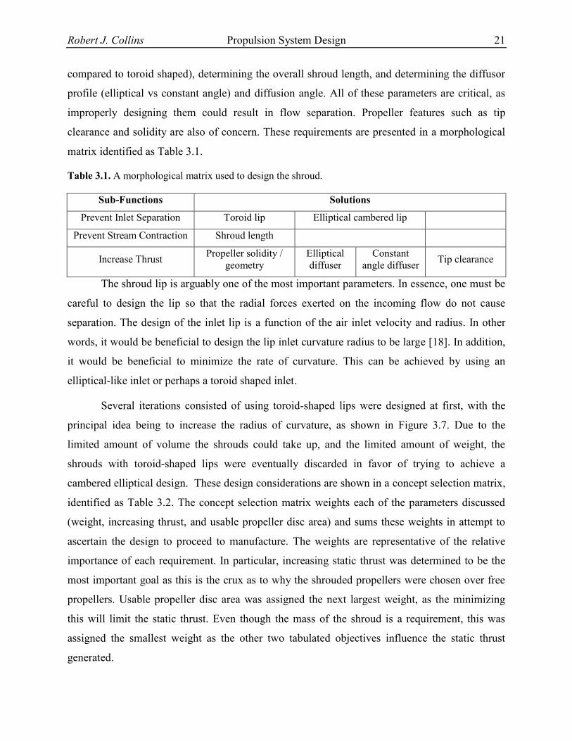
clearance and solidity are also of concern. These requirements are presented in a morphological
matrix identified as Table 3.1.
Table 3.1. A morphological matrix used to design the shroud.
Sub-Functions Solutions
Prevent Inlet Separation Toroid lip Elliptical cambered lip
Prevent Stream Contraction Shroud length
Increase Thrust Propeller solidity /
geometry
Elliptical
diffuser
Constant
angle diffuser Tip clearance
The shroud lip is arguably one of the most important parameters. In essence, one must be
careful to design the lip so that the radial forces exerted on the incoming flow do not cause
separation. The design of the inlet lip is a function of the air inlet velocity and radius. In other
words, it would be beneficial to design the lip inlet curvature radius to be large [18]. In addition,
it would be beneficial to minimize the rate of curvature. This can be achieved by using an
elliptical-like inlet or perhaps a toroid shaped inlet.
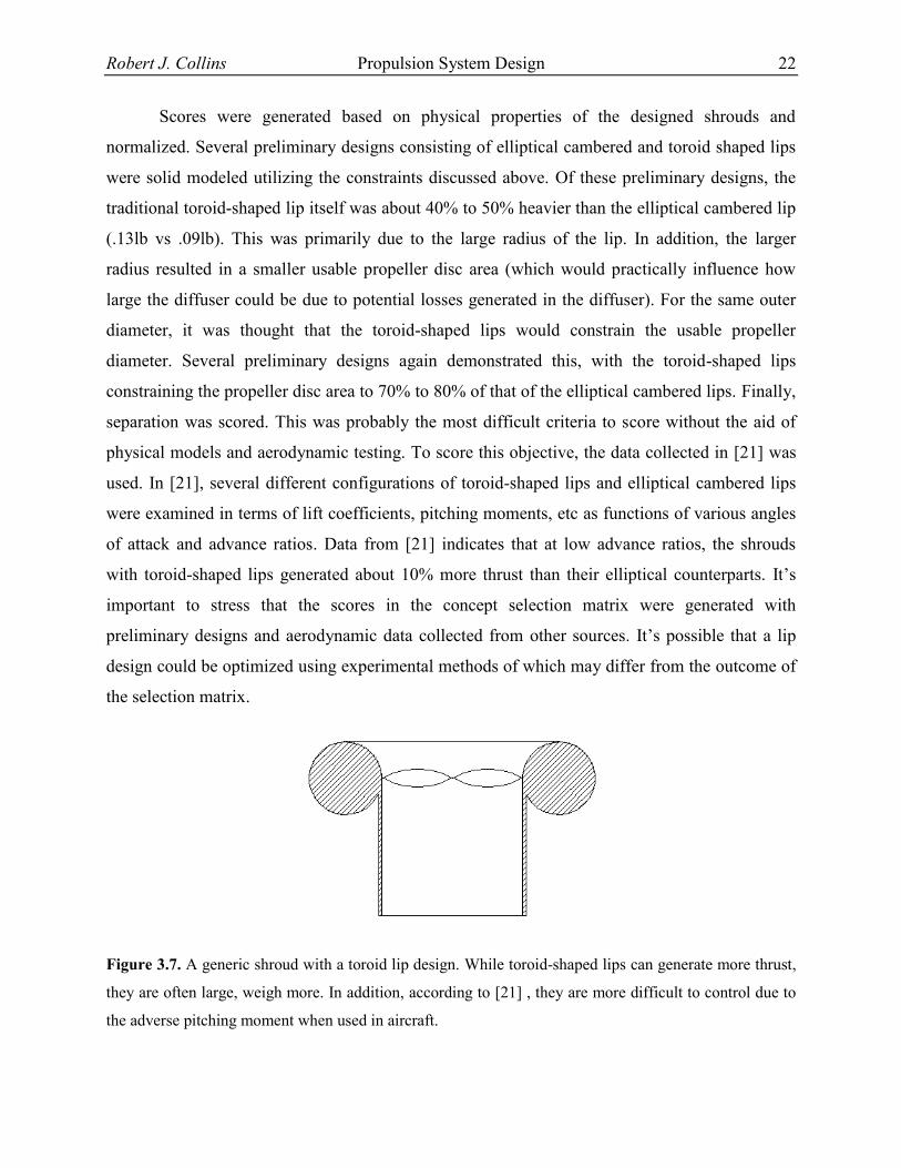
Several iterations consisted of using toroid-shaped lips were designed at first, with the
principal idea being to increase the radius of curvature, as shown in Figure 3.7. Due to the
limited amount of volume the shrouds could take up, and the limited amount of weight, the
shrouds with toroid-shaped lips were eventually discarded in favor of trying to achieve a
cambered elliptical design. These design considerations are shown in a concept selection matrix,
identified as Table 3.2. The concept selection matrix weights each of the parameters discussed
(weight, increasing thrust, and usable propeller disc area) and sums these weights in attempt to
ascertain the design to proceed to manufacture. The weights are representative of the relative
importance of each requirement. In particular, increasing static thrust was determined to be the
most important goal as this is the crux as to why the shrouded propellers were chosen over free
propellers. Usable propeller disc area was assigned the next largest weight, as the minimizing
this will limit the static thrust. Even though the mass of the shroud is a requirement, this was
assigned the smallest weight as the other two tabulated objectives influence the static thrust
generated.
Robert J. Collins Propulsion System Design 22
Scores were generated based on physical properties of the designed shrouds and
normalized. Several preliminary designs consisting of elliptical cambered and toroid shaped lips
were solid modeled utilizing the constraints discussed above. Of these preliminary designs, the
traditional toroid-shaped lip itself was about 40% to 50% heavier than the elliptical cambered lip
(.13lb vs .09lb). This was primarily due to the large radius of the lip. In addition, the larger
radius resulted in a smaller usable propeller disc area (which would practically influence how
large the diffuser could be due to potential losses generated in the diffuser). For the same outer
diameter, it was thought that the toroid-shaped lips would constrain the usable propeller
diameter. Several preliminary designs again demonstrated this, with the toroid-shaped lips
constraining the propeller disc area to 70% to 80% of that of the elliptical cambered lips. Finally,
separation was scored. This was probably the most difficult criteria to score without the aid of
physical models and aerodynamic testing. To score this objective, the data collected in [21] was
used. In [21], several different configurations of toroid-shaped lips and elliptical cambered lips
were examined in terms of lift coefficients, pitching moments, etc as functions of various angles
of attack and advance ratios. Data from [21] indicates that at low advance ratios, the shrouds
with toroid-shaped lips generated about 10% more thrust than their elliptical counterparts. It’s
important to stress that the scores in the concept selection matrix were generated with
preliminary designs and aerodynamic data collected from other sources. It’s possible that a lip
design could be optimized using experimental methods of which may differ from the outcome of
the selection matrix.
Figure 3.7. A generic shroud with a toroid lip design. While toroid-shaped lips can generate more thrust,
they are often large, weigh more. In addition, according to [21] , they are more difficult to control due to
the adverse pitching moment when used in aircraft.
Robert J. Collins Propulsion System Design 23
Table 3.2. Concept selection matrix of lip choices. The toroid and elliptical cambered lip are compared.
Toroid Lip Elliptical Cambered Lip
Objectives Weight (%) Score WS Score WS
Weight 20% .5 .1 1 .2
Increase Static Thrust
Output
50% 1 .5 .9 .45
Usable Propeller Disc
Area
30% .7 .21 1 .3
Total 100% .81 .95
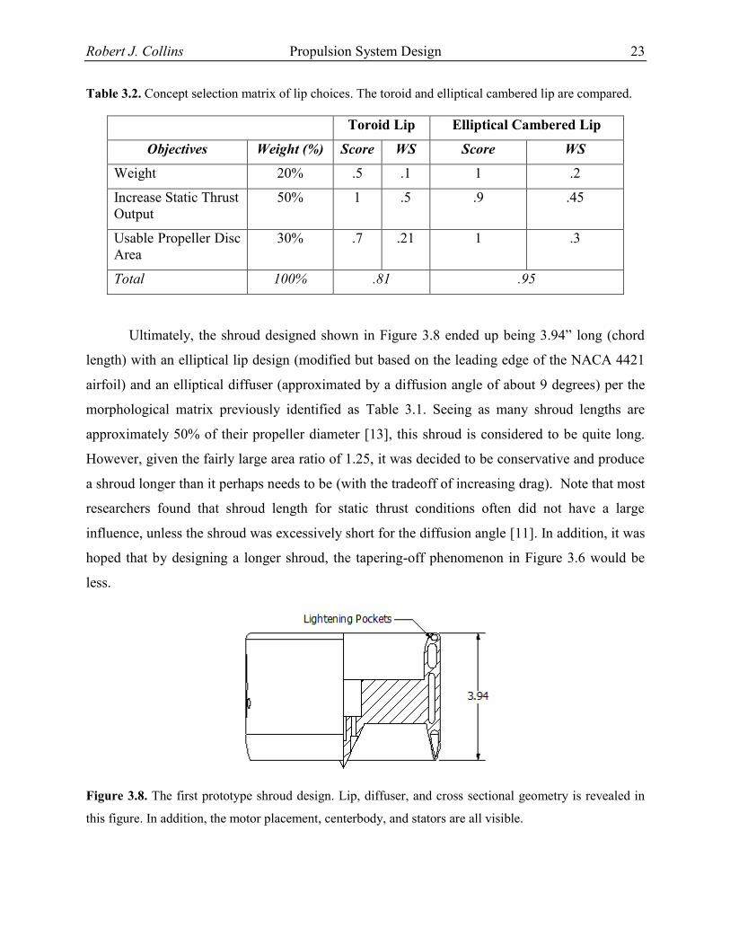
Ultimately, the shroud designed shown in Figure 3.8 ended up being 3.94” long (chord
length) with an elliptical lip design (modified but based on the leading edge of the NACA 4421
airfoil) and an elliptical diffuser (approximated by a diffusion angle of about 9 degrees) per the
morphological matrix previously identified as Table 3.1. Seeing as many shroud lengths are
approximately 50% of their propeller diameter [13], this shroud is considered to be quite long.
However, given the fairly large area ratio of 1.25, it was decided to be conservative and produce
a shroud longer than it perhaps needs to be (with the tradeoff of increasing drag). Note that most
researchers found that shroud length for static thrust conditions often did not have a large
influence, unless the shroud was excessively short for the diffusion angle [11]. In addition, it was
hoped that by designing a longer shroud, the tapering-off phenomenon in Figure 3.6 would be
less.
Figure 3.8. The first prototype shroud design. Lip, diffuser, and cross sectional geometry is revealed in
this figure. In addition, the motor placement, centerbody, and stators are all visible.
Robert J. Collins Propulsion System Design 24
In addition to the cross sectional shroud wall geometry, Figure 3.8 reveals the entire cross
sectional construction of the first prototype shroud that was tested. One of the first things to
notice is probably the hollow lightening pockets used in the wall cross section. This was done to
lighten the structure up considerably. This would normally be a manufacturing challenge as it
would perhaps require multiple pieces and molding / casting processes. However, it was decided
it would be easiest to fabricate the structure using an FDM rapid prototyping machine (printing
an ABS-like polymer). Using this machine, the shroud could be manufactured as a single part. In
addition, it would be easy for this machine to manufacture the lip / diffuser geometry (as
opposed to conventionally machining it, involving a multiple component assembly, tooling,
fixtures, and machine processes).
In addition to the lightening pockets, Figure 3.8 also illustrates the stator position and
chord length as well as the motor mount. The stators were designed to be a symmetrical and
constant chord in nature, with their principal purpose to support the motor and provide rigidity to
the structure. Stators can also be used to recover some of the thrust due to the propeller swirl, if
the angle of incidence is correct [21]. With the relatively low power consumption and thrust that
these shrouds would be generating, the angle of incidence of the stators was thought to be rather
small. After considering the theoretical results and the manufacturing implications, the stators
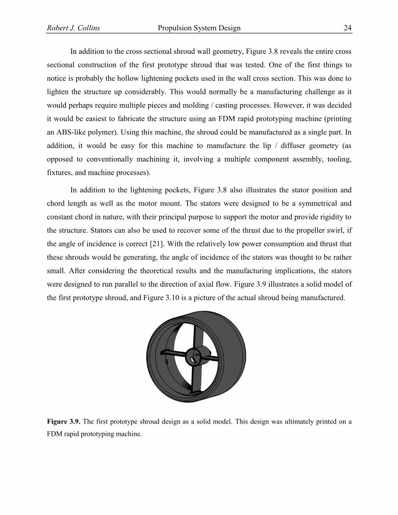
were designed to run parallel to the direction of axial flow. Figure 3.9 illustrates a solid model of
the first prototype shroud, and Figure 3.10 is a picture of the actual shroud being manufactured.
Figure 3.9. The first prototype shroud design as a solid model. This design was ultimately printed on a
FDM rapid prototyping machine.

Robert J. Collins Propulsion System Design 25
Figure 3.10. The first prototype shroud design being printed on a FDM rapid prototyping machine. The
machine is operated by the Virginia Tech DREAMS Laboratory.
As stated earlier, individual propeller design was felt to be outside the scope of this
thesis. Commercial propellers were instead bought and machined down to fit inside the shroud.
Due to the relative constant chord and three blades (resulting in a higher solidity ratio), a Master
Airscrew 3 bladed 8x6 propeller was machined down to an initial diameter of 4.98”.
3.3.3 Initial Shrouded Propeller Testing
With the shrouded propeller designed, the next logical step was to manufacture and test
it. In assembling the unit for testing, it was discovered that the diameter of the propeller was too
large for the shroud. With the shroud being nominally 5” in diameter and the propeller being
4.98” diameter, the propeller was certainly expected to fit inside the shroud with a small tip
clearance. Instead, it was found that the motor output shaft, and thus propeller were not perfectly
concentric, causing the propeller blades to collide with a section of the shroud wall if ran. In
addition to the shroud being not concentric, there were several other causes. These included the
motor mounting surface was uneven and not perpendicular to the direction of flow, and of
course, tolerances may not have been met by the FDM machine. The propeller ultimately had to
be machined down an additional .040” (off the diameter) in order to fit in the shroud. This
caused an uneven tip gap with the shroud.
Addressing this concern, the next step was to test the effectiveness of the shroud. This
was measured in several ways. First, the shrouded propeller assembly was tested to ensure the
flow field was staying attached and did not separate. Once this was confirmed, the shroud was
tested for total static thrust output, and characterized as a function of power and PWM.

Robert J. Collins Propulsion System Design 26
In order to make sure the flow was attached to the shroud walls, tufts were used to
visualize the flow. As seen in Figure 3.11, the flow appears to be attached at both the lip and the
diffuser for static thrust conditions. This indicates that the selected shroud geometry is working
effectively. To illustrate what separation looks like, an obstruction was placed near the shroud
inlet. The tufts during separation are shown in Figure 3.12.
Figure 3.11. Flow visualization - the flow field appears attached throughout the shroud. Left: The
prototype shroud inlet with tufts attached. Right: The same shroud, with tufts attached to the rear at the
diffuser. Separation does not appear to be an issue.
Figure 3.12. Separated flow field at the lip and diffuser. Notice the tufts are no longer streamlined,
indicative of separation. The separated flow field was caused by an obstruction being placed at the inlet.
It is worth noting that the noise level increased substantially when the flow was
separated. According to [12], shroud noise levels are indicative of the quality of flow attachment
to the shroud walls. In essence, one should expect a poorly designed shroud to be loud due to the
separation. Likewise, ensuring that the flow field remains attached will result in a quieter shroud.

Robert J. Collins Propulsion System Design 27
In addition to testing for flow field attachment, an “L” shaped balance was constructed to
measure the total thrust output of the shrouded propeller with a Honeywell Model 11 load cell.
Thrust data was acquired using a National Instruments 9234 DAQ and a small custom written
LabVIEW VI. Thrust data was collected as a function of rotation (RPM) and shaft power, and is
presented in Figure 3.13. Power was provided and measured by an Agilent E3632A power
supply. Rotational speed was adjusted by changing the duty cycle of the pulse width modulated
signal to the electronic speed controller of the motor. The rotational speed was measured by a
DT2234C digital laser tachometer. Notice that this shroud should meet both the thrust and power
requirements as discussed earlier. The shroud consumes about 50W at 100% throttle, and
produces .7lb of thrust.
Figure 3.13. Static thrust as a function of power and rotational speed of the propeller. The power curve is
shown in red while the rotational speed curve is shown in black. The trend observed is similar to the ideal
trend as presented in Figure 3.4.

Robert J. Collins Propulsion System Design 28
Figure 3.14. Figure of merit plotted as a function of rotational speed of the propeller.
In addition to plotting static thrust as a function of power and rotational speed of the
propeller, the figure of merit, as defined in equation 3.4, was calculated and plotted in Figure
3.14. Broadly, the figure of merit is a measure of efficiency, and compares the actual power to
induce the velocity through the propeller disc to the ideal power from momentum theory. It
should not be expected to have relatively high figures of merit, seeing as the Reynolds number at
75% of the radius of the propeller is quite low at 50,000. This Reynolds number suggests that
viscous drag will likely have a large impact on the performance.
√ (3.4)
These test results clearly indicate that the shrouded propeller designed will satisfy the
design requirements listed earlier in this chapter. However, recall that the primary deficiency is
the concentricity of the shroud, causing an excessive and uneven tip gap. To correct this, the
design had to be refined.
3.3.4 Final Shrouded Propeller Design
The shrouded propeller from the previous section was redesigned primarily to
compensate for the out of tolerance features resulting in a large tip gap. In essence, the same
aerodynamic shape was preserved, but the design of the individual shroud components changed.
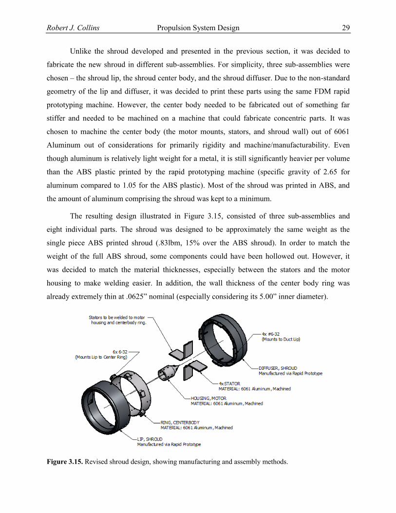
Robert J. Collins Propulsion System Design 29
Unlike the shroud developed and presented in the previous section, it was decided to
fabricate the new shroud in different sub-assemblies. For simplicity, three sub-assemblies were
chosen – the shroud lip, the shroud center body, and the shroud diffuser. Due to the non-standard
geometry of the lip and diffuser, it was decided to print these parts using the same FDM rapid
prototyping machine. However, the center body needed to be fabricated out of something far
stiffer and needed to be machined on a machine that could fabricate concentric parts. It was
chosen to machine the center body (the motor mounts, stators, and shroud wall) out of 6061
Aluminum out of considerations for primarily rigidity and machine/manufacturability. Even
though aluminum is relatively light weight for a metal, it is still significantly heavier per volume
than the ABS plastic printed by the rapid prototyping machine (specific gravity of 2.65 for
aluminum compared to 1.05 for the ABS plastic). Most of the shroud was printed in ABS, and
the amount of aluminum comprising the shroud was kept to a minimum.
The resulting design illustrated in Figure 3.15, consisted of three sub-assemblies and
eight individual parts. The shroud was designed to be approximately the same weight as the
single piece ABS printed shroud (.83lbm, 15% over the ABS shroud). In order to match the
weight of the full ABS shroud, some components could have been hollowed out. However, it
was decided to match the material thicknesses, especially between the stators and the motor
housing to make welding easier. In addition, the wall thickness of the center body ring was
already extremely thin at .0625” nominal (especially considering its 5.00” inner diameter).
Figure 3.15. Revised shroud design, showing manufacturing and assembly methods.
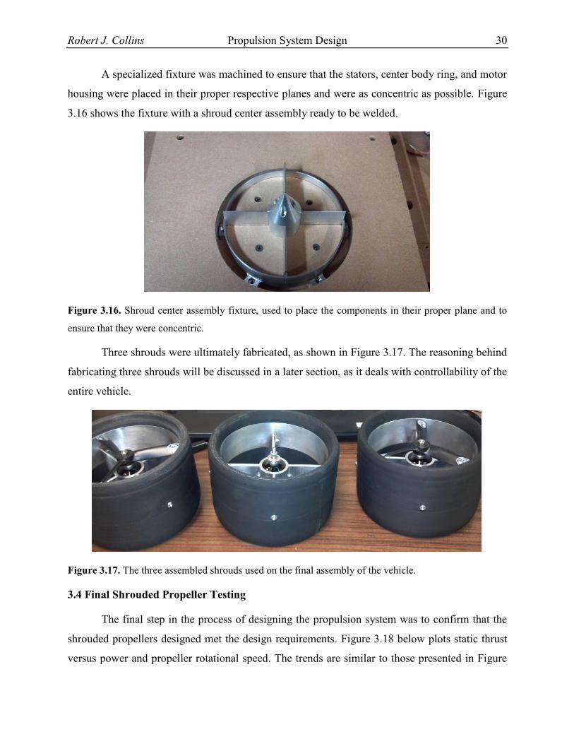
Robert J. Collins Propulsion System Design 30
A specialized fixture was machined to ensure that the stators, center body ring, and motor
housing were placed in their proper respective planes and were as concentric as possible. Figure
3.16 shows the fixture with a shroud center assembly ready to be welded.
Figure 3.16. Shroud center assembly fixture, used to place the components in their proper plane and to
ensure that they were concentric.
Three shrouds were ultimately fabricated, as shown in Figure 3.17. The reasoning behind
fabricating three shrouds will be discussed in a later section, as it deals with controllability of the
entire vehicle.
Figure 3.17. The three assembled shrouds used on the final assembly of the vehicle.
3.4 Final Shrouded Propeller Testing
The final step in the process of designing the propulsion system was to confirm that the
shrouded propellers designed met the design requirements. Figure 3.18 below plots static thrust
versus power and propeller rotational speed. The trends are similar to those presented in Figure

Robert J. Collins Propulsion System Design 31
3.13, with the maximum static thrust of the final design roughly the same as the prototype
design.
Figure 3.18. Static thrust as a function of power and rotational speed of the propeller. The error bars
show two standard deviations.
With each shroud requiring about 43W of power at full throttle, the design power
requirements are met. However, the design requirement of being able to produce 1.0lb of thrust
is not met by using a single shroud. It is likely two shrouds will be needed to be able to produce
1.0lb to avoid wall / obstacle collisions. This isn’t so much of a concern, as overall vehicle
stability will require multiple thrusters / shrouds.
The final step in characterizing the shroud required a relationship to be developed
between static thrust and the pulse width modulated signal duration. Electronic speed controllers
control the RPM of the attached motor by receiving a pulse width modulated signal. The
controller that was designed for this vehicle (presented in a later section) requires knowledge of
this relationship. Figure 3.19 shows the relationship of static thrust as a function of the pulse
width modulated signal duty cycle.
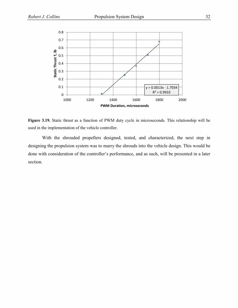
Robert J. Collins Propulsion System Design 32
Figure 3.19. Static thrust as a function of PWM duty cycle in microseconds. This relationship will be
used in the implementation of the vehicle controller.
With the shrouded propellers designed, tested, and characterized, the next step in
designing the propulsion system was to marry the shrouds into the vehicle design. This would be
done with consideration of the controller’s performance, and as such, will be presented in a later
section.
y = 0.0013x - 1.7034 R² = 0.9933
0
0.1
0.2
0.3
0.4
0.5
0.6
0.7
0.8
1000 1200 1400 1600 1800 2000
Stat
ic T
hru
st T
, lb
PWM Duration, microseconds

Robert J. Collins Wall Detection 33
Chapter 4 Wall Detection
Designing a helicopter-deployable vehicle for supplying ground units requires many sub-
systems. In particular, such a vehicle would need an environmental detection system to detect
walls for the ultimate goal of avoiding collisions with the surrounding environment. In this
particular case, the vehicle will use a Hokuyo URG-04LX scanning laser range finder unit for
detection.
It’s important to note that many different detection techniques could be used such as
utilizing various vision algorithms / systems. However, many of these vision systems require a
large amount of computational horsepower; provide too much information, or both. For this
particular vehicle, the obstacles / walls at the vehicle’s altitude are the only concern. This implies
that the vehicle will only need a 2D point map (excluding height information). Utilizing an
instrument that only collects 2D information will also decrease the computational requirements
of the vehicle’s onboard computer. The URG-04LX scanning laser range finder collects 2D
information only, making it an ideal candidate in light of this discussion. This chapter discusses
the design and implementation of the wall detection / tracking system utilizing the URG-04LX.
4.1 System Requirements
In addition to physical hardware to acquire the data, software is a necessity in the
detection of walls and the surrounding environment. In order to have a reliable detection system,
several requirements must be met.
The detection algorithm must be able to report distance to and angle to the wall
precisely. With the control scheme utilizing and controlling the distance and angle to a
wall, excessive noise is an unacceptable issue. If the distance and angle measurements are
noisy, the controller will likely be oscillating to compensate for dynamics that aren’t
really occurring. A filter will likely have to be used to compensate for some noise.
The detection algorithm must be able to find a window. It is conceivable that a vehicle
like this could be used in delivering supplies or extracting equipment / people / hardware.
In addition, the vehicle could also be outfitted with specialized payloads for mission
specific tasks. For example, imaging equipment could be outfitted on the vehicle for
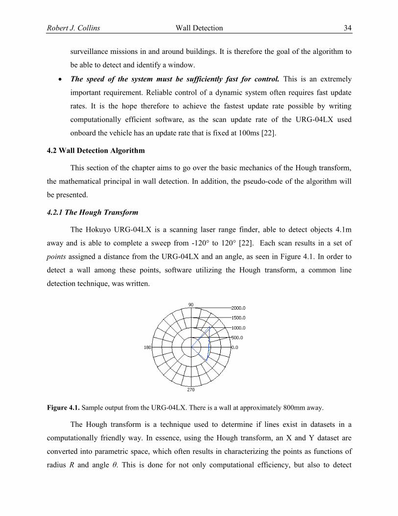
Robert J. Collins Wall Detection 34
surveillance missions in and around buildings. It is therefore the goal of the algorithm to
be able to detect and identify a window.
The speed of the system must be sufficiently fast for control. This is an extremely
important requirement. Reliable control of a dynamic system often requires fast update
rates. It is the hope therefore to achieve the fastest update rate possible by writing
computationally efficient software, as the scan update rate of the URG-04LX used
onboard the vehicle has an update rate that is fixed at 100ms [22].
4.2 Wall Detection Algorithm
This section of the chapter aims to go over the basic mechanics of the Hough transform,
the mathematical principal in wall detection. In addition, the pseudo-code of the algorithm will
be presented.
4.2.1 The Hough Transform
The Hokuyo URG-04LX is a scanning laser range finder, able to detect objects 4.1m
away and is able to complete a sweep from -120° to 120° [22]. Each scan results in a set of
points assigned a distance from the URG-04LX and an angle, as seen in Figure 4.1. In order to
detect a wall among these points, software utilizing the Hough transform, a common line
detection technique, was written.
Figure 4.1. Sample output from the URG-04LX. There is a wall at approximately 800mm away.
The Hough transform is a technique used to determine if lines exist in datasets in a
computationally friendly way. In essence, using the Hough transform, an X and Y dataset are
converted into parametric space, which often results in characterizing the points as functions of
radius R and angle θ. This is done for not only computational efficiency, but also to detect

Robert J. Collins Wall Detection 35
vertical lines. For example, characterizing these points as functions of slope and the vertical axis
intercept would lead to problems when a detected line is vertical. To find a common collinear
line between these points, many lines are drawn through the point of interest by iterating θ a
discrete amount in equation 4.1. The results (an angle and distance of a line drawn through each
point) are stored in an array, typically referred to as an accumulator. The accumulator is then
examined to look for a common distance R and angle θ within a specified tolerance. A voting
scheme is used to analyze the accumulator array to “vote” for common distances and angles. If
the number of votes exceeds a certain threshold, a line is claimed to be found [14].
( ) ( ) (4.1)
To help visualize the mechanics of the Hough transform, a plot can be created relating
line distance R to angle θ (typically referred to as the Hough space) of the data set. Figures 4.2
and 4.3 illustrate a sample data set and the Hough space of the sample data set. Figure 4.2 is a
plot of a line consisting of seven data points with a slope of -1 and a vertical intercept of 1.
Figure 4.2. A sample data set having a slope of -1 and a y-intercept of 1. All of the sample data points
reside along the line, which will be evident in the Hough space.

Robert J. Collins Wall Detection 36
Figure 4.3. The Hough space of the sample data set presented in Figure 4.2. The distance from the origin
and corresponding angle can be identified.
The Hough space is a plot of all of the interested distances (from the origin) as functions
of angle of the “ith
” data point. If the points are collinear, the Hough space of the data set should
converge to a particular distance R and angle θ. As shown in Figure 4.3, this is the case. With all
of the points residing on the same line, it is quite evident that the distance from the line to the
origin is about .71 while the angle is 45 degrees.
In a real world environment, the data set acquired from the Hokuyo laser range finder
could potentially contain no walls, other obstacles, or multiple walls. Developing step sizes for
the angle, range, and tolerances for the voting scheme are necessary to accurately detect a wall
and the respective position. Improperly placed tolerances and step sizes can result in noisy data
and incorrect identification of a wall. Since the controller will be using the data processed from
the Hough transform to control its yaw angle and distance, the measurements must be relatively
noise free and accurate.
4.2.2 Wall Detection Algorithm Pseudo-Code
The wall detection algorithm used in the development of the supply vehicle makes use of
the Hough transform presented in the previous sub-section. The wall detection code was written
in LabVIEW 2010 (to take advantage of the Hokuyo driver written for LabVIEW). Since
LabVIEW is a data flow oriented language utilizing wires and block diagrams and is hard to
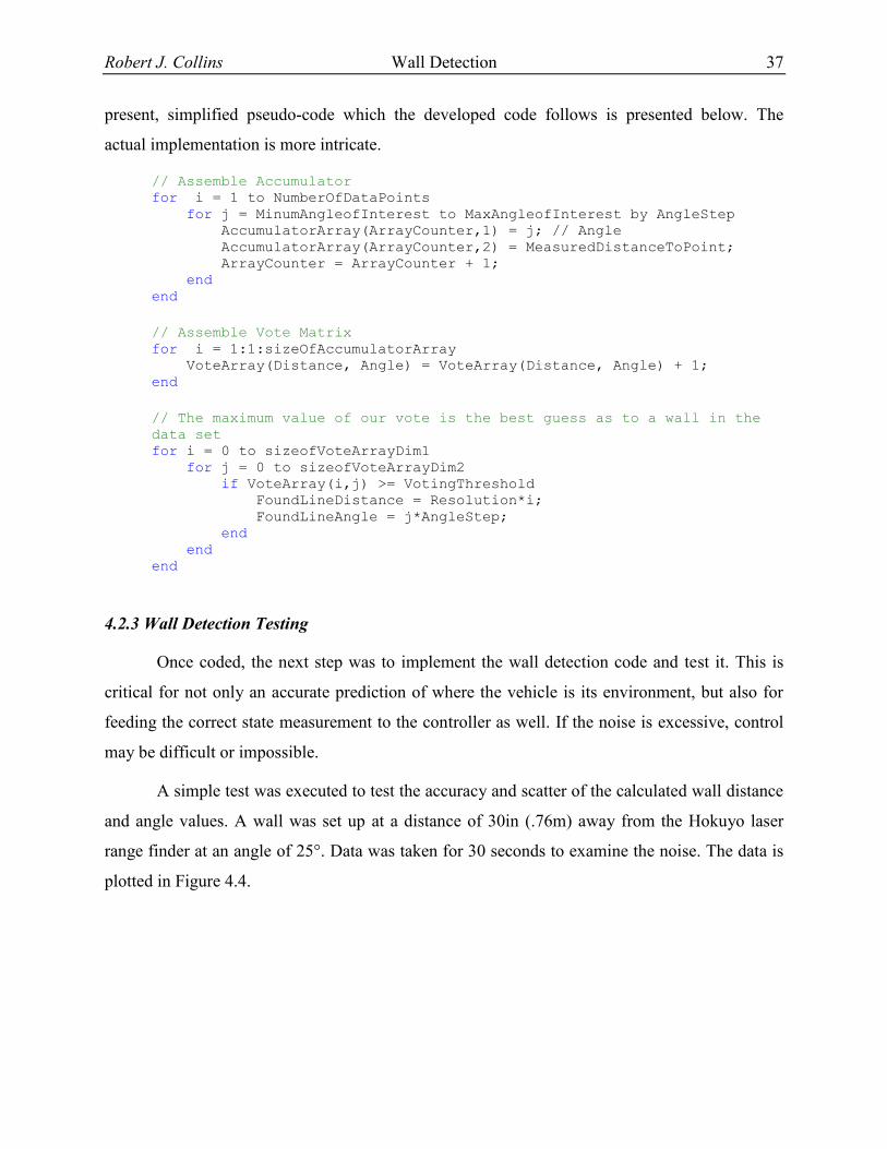
Robert J. Collins Wall Detection 37
present, simplified pseudo-code which the developed code follows is presented below. The
actual implementation is more intricate.
// Assemble Accumulator for i = 1 to NumberOfDataPoints for j = MinumAngleofInterest to MaxAngleofInterest by AngleStep AccumulatorArray(ArrayCounter,1) = j; // Angle AccumulatorArray(ArrayCounter,2) = MeasuredDistanceToPoint; ArrayCounter = ArrayCounter + 1; end end
// Assemble Vote Matrix for i = 1:1:sizeOfAccumulatorArray VoteArray(Distance, Angle) = VoteArray(Distance, Angle) + 1; end
// The maximum value of our vote is the best guess as to a wall in the
data set for i = 0 to sizeofVoteArrayDim1 for j = 0 to sizeofVoteArrayDim2 if VoteArray(i,j) >= VotingThreshold FoundLineDistance = Resolution*i; FoundLineAngle = j*AngleStep; end end end
4.2.3 Wall Detection Testing
Once coded, the next step was to implement the wall detection code and test it. This is
critical for not only an accurate prediction of where the vehicle is its environment, but also for
feeding the correct state measurement to the controller as well. If the noise is excessive, control
may be difficult or impossible.
A simple test was executed to test the accuracy and scatter of the calculated wall distance
and angle values. A wall was set up at a distance of 30in (.76m) away from the Hokuyo laser
range finder at an angle of 25°. Data was taken for 30 seconds to examine the noise. The data is
plotted in Figure 4.4.

Robert J. Collins Wall Detection 38
Figure 4.4. Sample record of distance and angle, calculated by the wall detection algorithm. The wall
detection algorithm appears to detect the test wall at about .76m at an angle of 25°.
The results of the test plotted in Figure 4.4 indicate that the wall detection algorithm is
able to successfully detect a wall at about .76m at an angle of 25°. Both subplots indicate there is
some degree of noise to the measurement. However, with the algorithm detecting a wall at an
average of .766m (.008m standard deviation) at 24.8° (.979° standard deviation), it shouldn’t be
an issue to the controller with a filter on it. It should be noted that the wall detection algorithm
used an angular step size of 2° and a 4mm distance resolution. These numbers were chosen by
iteration, with considerations mostly given towards computation time.
In addition to testing for functionality and noise, the performance of the actual
implementation of the wall detection algorithm was measured. The start-to-finish iteration time
was collected via LabVIEW’s Performance Profiler for a few sample data sets. These results are
displayed in Table 4.1. It is important to note that the time logged for each trial represents the
start-to-finish runtime of the VI and therefore does not include acquisition times. This test was
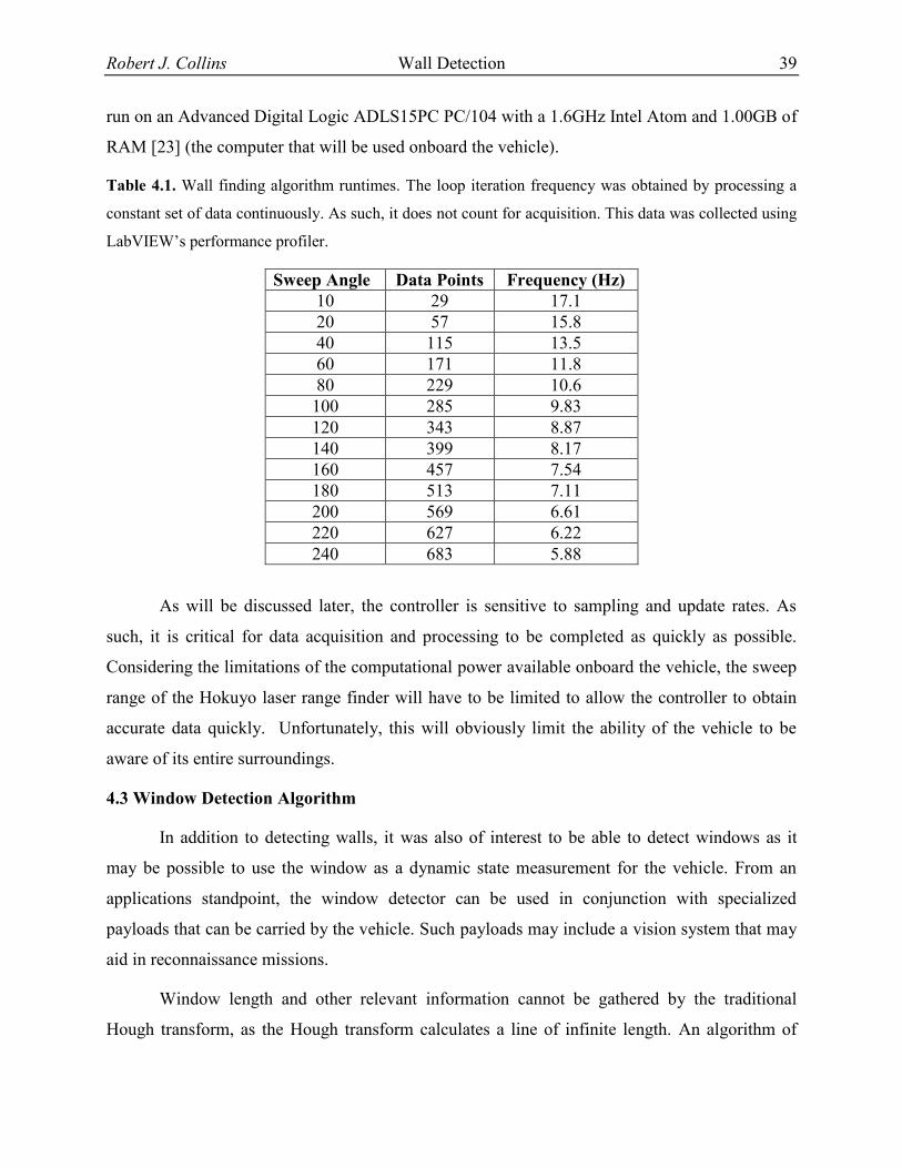
Robert J. Collins Wall Detection 39
run on an Advanced Digital Logic ADLS15PC PC/104 with a 1.6GHz Intel Atom and 1.00GB of
RAM [23] (the computer that will be used onboard the vehicle).
Table 4.1. Wall finding algorithm runtimes. The loop iteration frequency was obtained by processing a
constant set of data continuously. As such, it does not count for acquisition. This data was collected using
LabVIEW’s performance profiler.
Sweep Angle Data Points Frequency (Hz)
10 29 17.1
20 57 15.8
40 115 13.5
60 171 11.8
80 229 10.6
100 285 9.83
120 343 8.87
140 399 8.17
160 457 7.54
180 513 7.11
200 569 6.61
220 627 6.22
240 683 5.88
As will be discussed later, the controller is sensitive to sampling and update rates. As
such, it is critical for data acquisition and processing to be completed as quickly as possible.
Considering the limitations of the computational power available onboard the vehicle, the sweep
range of the Hokuyo laser range finder will have to be limited to allow the controller to obtain
accurate data quickly. Unfortunately, this will obviously limit the ability of the vehicle to be
aware of its entire surroundings.
4.3 Window Detection Algorithm
In addition to detecting walls, it was also of interest to be able to detect windows as it
may be possible to use the window as a dynamic state measurement for the vehicle. From an
applications standpoint, the window detector can be used in conjunction with specialized
payloads that can be carried by the vehicle. Such payloads may include a vision system that may
aid in reconnaissance missions.
Window length and other relevant information cannot be gathered by the traditional
Hough transform, as the Hough transform calculates a line of infinite length. An algorithm of

Robert J. Collins Wall Detection 40
this nature can also be used to detect portals, the edges of walls, etc. This section of the chapter
discusses how window detection / finite line detection was implemented.
4.3.1 Window Detection Algorithm and Pseudo-Code
Even though the Hough transform calculates a line infinitely long in length, the data set
used to calculate the direction and distance of the wall / line is finite. To detect a window in the
infinitely long line, the algorithm must first calculate the distance from each data point of interest
to the found line (wall). Since it is expected that there will be noise in the data set, these points
are compared to a distance threshold to determine if they actually represent the wall. If any of
these points exceed the threshold, they most likely aren’t part of the wall and might be a window.
The indices of the first data point and last data point that do not exceed the distance threshold
from the wall are then stored. Knowing these points, respective X and Y coordinates, the
distance of the break in the line (possibly the assumed window) can be easily calculated. The
break can then be compared to another threshold to determine if the break is indeed a window of
typical size.
Like the wall detection algorithm, this algorithm was written in LabVIEW 2010. It is
implemented as a subVI / function that will be called as part of the control routine. Pseudo-code
of the basic algorithm is listed below.
% Throw away points that are far away from the found line for i = 1:AmountofDataPoints if DistanceFromPointToFoundLine < ThresholdLine DistanceFromLine(i) = CalculatedDistanceFromLine; else DistanceFromLine(i) = 0; end end
% Calculate the distance between for i = 1:AmountofDataPoints if DistanceFromLine(i) >0 DistanceBetweenPoints(i) = Distance_i_to_iinc1 end end
4.3.2 Window Detection Testing
With the window detection algorithm coded, the next step was to quantify its
performance by testing it. The window detection algorithm was tested by placing a “window” in

Robert J. Collins Wall Detection 41
the wall measuring 18.25 in (.464 m) across. To see if the measurement and calculation contain
significant noise, the calculated window width over time is plotted in Figure 4.5.
Figure 4.5. Sample record of detected window width. The window detection algorithm successfully
detected a window at about .463m. One extreme outlier is shown in this data set.
As seen in Figure 4.5, the window detection algorithm detected a break / window in the
test wall. The average window width of the time of the sample was .463m with a standard
deviation of .0125m. This agrees with the test setup of 18.25in (.464m). It should be noted that
the window detection algorithm was tested with 171 data points and executed in a negligible
1.2ms. While this figure does not include acquisition time, it does include the time it takes to
draw and update the indicators and controls on the VI. Since this will be executed as a SubVI in
most situations, the execution time will be far less – on the order of .17ms.

Robert J. Collins Tethered Supply Vehicle Design 42
Chapter 5 Tethered Supply Vehicle Design
With the subassemblies / systems designed, the next step was to incorporate all of these
subsystems into a single, controllable, tethered vehicle. This chapter discusses the design
decisions and process of the tethered resupply vehicle.
5.1 Vehicle Requirements
Before the assembly was modeled and designed, the requirements of the vehicle needed
to be identified. They are:
The vehicle must meet weight restrictions. A typical 100kg class helicopter, like one
that may be used in the proposed resupply scenario will realistically will have
approximately 10kg worth of payload capacity before exceeding its allowable gross
weight. It is desired to budget at least half of this 10kg payload capacity for the
hypothetical supplies, with the other 5kg budgeted for the vehicle itself. It is therefore
desired to design a vehicle weighing 5kg or less.
The vehicle must meet the geometric constraints of the USL developed winch. The
USL developed winching system is designed to be attached to the Yamaha RMAX
helicopter flown by the lab. Originally designed to deploy a ground sampling /
collection robot, it is desired to use the winch for the deployment of other tethered
vehicles such as this one. To use the currently designed winch system, the vehicle
must first be able to fit in the confined space under the helicopter. This volume
measures approximately 19”x19”x9”.
The vehicle must carry computing power and all necessary sensors onboard. The
main goal of this vehicle is to be able to deliver supplies precisely where needed. In
addition, it is desired to be able to use the sensor data collected by the vehicle to
avoid obstacles if need be. Simply being tethered to the helicopter, it is desired to do
all processing onboard if possible for control. Likewise, sensors will need to be
onboard the vehicle as well to provide dynamic measurements (yaw, yaw rate,
velocity, etc). In addition, a LIDAR / laser range finder will need to be placed
Robert J. Collins Tethered Supply Vehicle Design 43
onboard the vehicle to collect information about walls, windows, and potential
obstacles.
The vehicle must be controllable. Perhaps the most important practical requirement,
the vehicle must be able to control itself using a feedback loop. This directly dictates
the vehicle design as thruster placements, the center of mass, the rotation point, etc all
govern the dynamics of the vehicle that must be controlled. For example, since the
vehicle must be able to rotate under its own power (let’s say to follow a wall), the
thrusters must be positioned to generate a torque. In addition, since it is desired to
have .1g of horizontal acceleration to avoid a wall, the thrusters must be positioned to
generate enough thrust. It is for these reasons that some of the basic controller design
must be developed along with to design the vehicle.
The vehicle must be able to carry a small payload. This requirement is one of the
primary goals of designing this vehicle – to be able to deliver a payload to a precise
location. However, considering that the vehicle will need to have thrusters, a
computer and other instrumentation, and is limited by the geometric constraints of the
Yamaha RMAX and winch system, there is a very limited amount of area for a
payload. It is desired to maximize the amount of area available to secure supplies to
the vehicle.
The vehicle’s structure must be able to support a payload and all of the sub
systems. With 5kg worth of payload and the vehicle itself weighing 5kg, the vehicle
must be able to adequately support the payload carried by it and all sensors /
mechanical equipment. Excessive deflection and inadequate stiffness could
potentially cause problems with the controller, having to account for additional
dynamics.
The vehicle must be able to operate in a GPS denied environment. One of the
proposed mission scenarios of this vehicle is to be able to deliver supplies in an urban
area. While GPS (Global Positioning System) satellite signals are often times
receivable and many GPS units function in an urban area (such as the commercially
available units to provide driving directions), position and velocity accuracy can
significantly degrade. It is for this reason that it is desired to not rely on any of the
position or velocity states of the vehicle by GPS.

Robert J. Collins Tethered Supply Vehicle Design 44
5.2 Vehicle Electronics and System Architecture
In order to meet the previously developed requirements and goals, the vehicle will need
to have several sensors, microcontrollers, etc. This section of the chapter details the electronic
hardware and how all of the systems were bridged together.
5.2.1 Navigational System
As previously detailed in chapter 4 of this thesis, a Hokuyo laser range finder (URG-
04LX) was used to detect walls along the vehicle’s path. Even though the perpendicular distance
to the wall and the respective angle are important measurements and states to have, they alone
are not sufficient. Translational and rotational position and velocity information are also
required. This information can be gained in several ways – one, by an inertial measurement unit,
and two, some position and velocity information can be provided by a GPS. However, per the
requirements listed in the previous section of this chapter, outfitting the vehicle with a GPS is not
permitted. Measuring and calculating these states therefore requires an IMU on the vehicle.
A MicroStrain 3DM-GX2, pictured in Figure 5.1, was selected for use as an onboard
IMU. This particular unit is capable of outputting accelerations in the X, Y, and Z direction (and
the integrated velocities). In addition, it is also capable of outputting yaw, pitch, roll, and all of
their respective rates. This IMU communicates via RS232 at 115.2kbps and is capable of
providing updates at 250Hz [24].
Figure 5.1. A picture of the MicoStrain 3DM-GX2 IMU. This unit will be mounted onboard the supply
vehicle to gather the dynamic states of the vehicle.
5.2.2 Vehicle Onboard Computer
As briefly stated in Chapter 4, the tethered supply vehicle was outfitted with an
Advanced Digital Logic ADLS15PC PC104 computer. This computer has a 1.6GHz Intel Atom

Robert J. Collins Tethered Supply Vehicle Design 45
processor with 1.00GB of RAM [23]. In addition, this computer was outfitted with a solid state
hard drive.
The ADLS15PC PC104 was selected for two primary reasons. First, the computer is
capable of running Microsoft Windows on it. Second, the URG-04LX laser range finder is easy
to communicate with using LabVIEW (installed on Windows) as the acquisition SubVIs were
already written by Hokuyo. The disadvantage to this approach is that Windows is not a real-time
operating system, and as such, running a program at a specific desired rate may be difficult.
The ADLS15PC PC104 pictured in Figure 5.2 is relatively small. The board measures
about 4” x 3.5”. This does not include the power supply board, which is also similar in size.
However, the bus pins are rather long, which will probably require the computer housing / case
to have a significant height. This computer features two serial ports and more than eight USB
ports, which is more than enough for the acquisition needs of this vehicle.
Figure 5.2. A picture of the ADLS15PC PC104. This picture does not feature the power supply board.
5.2.3 Propulsion System Electronics
Even though the propulsion system hardware was designed at selected at this point
(Chapter 3), the electronic hardware to control the motors and communicate to the onboard
computer had not been selected. In chapter 3, Hacker out runner motors were selected. These
motors are typically controlled with electronic speed controllers, such as the Castle 25 selected
and used. However, these electronic speed controllers are normally used with small-scale hobby
aircraft receivers. As such, these controllers control the speed of the motor by receiving a pulse
width modulated input signal. In order to send a digital signal to the electronic speed controller, a
small microcontroller is necessary (the ADLS15PC PC104 does not have any digital input or

Robert J. Collins Tethered Supply Vehicle Design 46
output pins). An Arduino MEGA (shown in Figure 5.3) utilizing the ATmega1280 was selected
to provide this functionality. Selection was primarily based on the hardware available in the lab
as this board has 14 PWM outputs, far more than is required.
Figure 5.3. A picture of the Arduino MEGA. The Arduino MEGA was selected to provide a pulse width
modulated signal to the electronic speed controllers.
5.2.4 Wireless Communication
It is necessity to be able to communicate with the tethered supply vehicle to perform a
variety of functions (turn the controller on/off, to identify windows, for debugging, etc). Seeing
as the vehicle is tethered and self-powered, a wireless communication method is necessary. An
802.11n external USB wireless card was used to provide this functionality.
5.2.5 System Architecture Overview
With a variety of sensors and subsystems onboard the tethered supply vehicle identified,
the next step was to ensure all of them functioned reliably in concert. In order to achieve this
requirement, the first step was to identify how all of the subsystems and instrumentation would
communicate. This is shown in Figure 5.4 - a block diagram of the entire vehicle’s architecture.

Robert J. Collins Tethered Supply Vehicle Design 47
Figure 5.4. Block diagram of the system architecture. Note that the arrows show the primary direction of
the flow of data.
As seen from the block diagram in Figure 5.4, the PC104 is used to collect data from the
IMU by serial and the laser range finder (USB). The PC104 is then able to determine the
dynamic state of the vehicle (position from the wall, velocity, angle from the wall, angular rate,
etc) by executing the Hough transform / wall detection algorithm. Using a control loop executed
on the PC104, a serial message to the ATmega1280 with regard to the length of the pulse width
modulated signal needed to achieve a particular thrust (relationship shown in Figure 3.19). The
custom written program on the Arduino outputted PWM signals that were received by the
electronic speed controllers. Once the signal was received, the ESCs adjusted the rotational
speed, and thus thrust output, of the shrouded propellers / ducted fans. The ground computer
(could perhaps also be a computer onboard the helicopter) is able to turn on and off the control
algorithm and issue other open-loop commands via the 802.11n wireless adapter onboard.
Most of the executable code on the PC104 was written in LabVIEW 2010. While other
languages are certainly faster, LabVIEW 2010 was chosen to take advantage of Hokuyo’s pre-

Robert J. Collins Tethered Supply Vehicle Design 48
written driver to acquire data from the URG-04LX. Code was also written for the ATmega1280
using a C variant published by Arduino.
Since the vehicle is going to be self-powered and contained, it is important to get a sense
of the total power consumption to properly size the batteries. With the motors turned off and the
vehicle running just the computer and all sensors, the total power consumption was measured to
be 20.8W. With each motor running at full throttle and all systems powered up, the total power
consumption of the vehicle was measured at 170W.
5.3 Design and Implementation of Software User Interface
Custom software was written and implemented on the PC104 onboard the tethered supply
vehicle. This software ultimately collected the laser range finder data, IMU data, communicated
to the ATmega1280, and provided a remote desktop connection for the ground computer. Figure
5.5 shows a screen shot to what the user would see. In normal operation, the user would simply
select to turn on and off the controller. The IMU data, laser range finder data, etc, would then be
updated every iteration of the control loop automatically. As seen in Figure 5.5, the program is
also able to collect the IMU and laser range finder data manually, mostly for debugging
purposes.

Robert J. Collins Tethered Supply Vehicle Design 49
Figure 5.5. Screenshot of the user interface for the tethered supply vehicle. The user can view in real time
the environment as acquired by the laser ranger finder, log states, and enable the controller.
The main screen shown in Figure 5.5 is the only LabVIEW VI the user will have to
interact with on a normal basis. There are over twenty custom-written virtual instruments though,
most of them acting as SubVIs to provide complete functionality.
5.4 Dynamic System Modeling
Before any mechanical design can be done, the requirement of controllability must be
addressed. To address this issue, a simple dynamic model was constructed with a full state
feedback controller. Simulations were executed iteratively; comparing settling time as the
physical parameters of a vehicle platform were varied (thrust angles and positions, moment arms,
etc). This section of the chapter discusses the dynamic system modeling used for the design of
the tethered vehicle. A more in depth explanation of the dynamics will be given in the next
chapter.
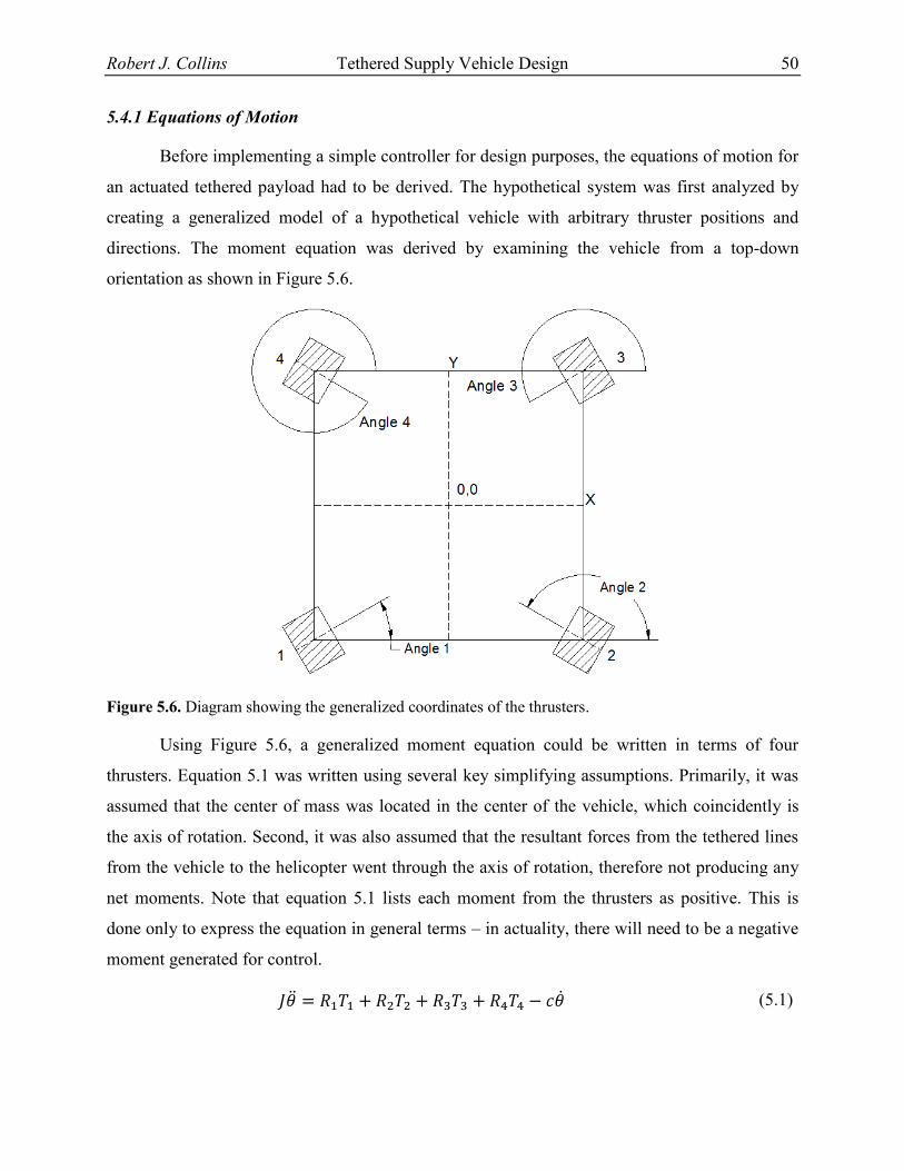
Robert J. Collins Tethered Supply Vehicle Design 50
5.4.1 Equations of Motion
Before implementing a simple controller for design purposes, the equations of motion for
an actuated tethered payload had to be derived. The hypothetical system was first analyzed by
creating a generalized model of a hypothetical vehicle with arbitrary thruster positions and
directions. The moment equation was derived by examining the vehicle from a top-down
orientation as shown in Figure 5.6.
Figure 5.6. Diagram showing the generalized coordinates of the thrusters.
Using Figure 5.6, a generalized moment equation could be written in terms of four
thrusters. Equation 5.1 was written using several key simplifying assumptions. Primarily, it was
assumed that the center of mass was located in the center of the vehicle, which coincidently is
the axis of rotation. Second, it was also assumed that the resultant forces from the tethered lines
from the vehicle to the helicopter went through the axis of rotation, therefore not producing any
net moments. Note that equation 5.1 lists each moment from the thrusters as positive. This is
done only to express the equation in general terms – in actuality, there will need to be a negative
moment generated for control.
(5.1)

Robert J. Collins Tethered Supply Vehicle Design 51
In addition to equation 5.1, an equation to relate the vehicle’s position from the wall was
necessary. Again, using Figure 5.6 and Figure 5.7, a force balance (equation 5.2) was written in
terms of the thrusters and the mass of the vehicle. In addition to accounting for thrusters, small
deflection linear pendulum dynamics were incorporated in the “x” direction. More detail on this
derivation can be found in the next chapter.
Figure 5.7. Diagram showing 2D pendulum motion.
( ) ( ) ( ) ( )
(5.2)
With equations 5.1 and 5.2 derived, the perpendicular distance and angle from the wall
could be controlled. These equations are reassembled into state space form as shown in equation
5.3.
[
]
[
]
[
]
[
( ( )
) (
( )
) (
( )
) (
( )
)]
[
] (5.3)
5.4.2. Thruster Placement for Controllability
With the equations of motion / equation 5.3 derived, it was possible to design a vehicle
for controllability. First, a Simulink model was created utilizing the state space equation listed

Robert J. Collins Tethered Supply Vehicle Design 52
equation 5.3 and a full state feedback controller, utilizing the control law –Ku in the feedback
loop. Saturation limits were put in place to limit the actuation of the thrusters (shrouded
propellers / ducted fans) between 0 and the top end limit of 3.3N. The Simulink model is shown
in Figure 5.8.
Figure 5.8. Original Simulink model used to design the vehicle for controllability.
Once the Simulink model shown in Figure 5.8 was created, a MATLAB code was written
to utilize the model. This MATLAB code iterated the physical parameters of the vehicle for a
given set of poles and initial conditions and logged the settling time (time it took for each state to
reach 0 to within 2%). The calculated results from the MATLAB code had to be balanced with
the requirements of the vehicle. For example, depending on the initial conditions of the vehicle,
the MATLAB script may have optimized the thrusters to be in a position to minimize settling
time turning in a particular direction, but leave the vehicle with little control authority if it
needed to turn the opposite direction.
It was ultimately decided to design a tethered vehicle with a three-thruster arrangement.
While a fourth thruster would arguably provide more control authority if oriented properly, it
was decided to use a three-thruster arrangement to minimize weight. By sticking to three
thrusters, the entire propulsion system would only contribute 2.97lb to the entire vehicle weight
(less than the 4lb requirement discussed previously in Chapter 3). The thruster placement
configuration chosen featured two fixed shrouds and one with a vectoring mechanism. The thrust
vectoring shroud will allow the vehicle to output .1g in a direction. However, because a

Robert J. Collins Tethered Supply Vehicle Design 53
linearized model was used (equations 5.1, 5.2), thrust vectoring was not incorporated in the
current controller. It was decided to “lock” the vectoring mechanism at a particular angle for
testing. The final design geometric parameters are shown in Table 5.1. These measurements are
based off of the geometric parameters shown in Figure 5.6.
Table 5.1. Thruster placement parameters, *indicates thrust vectoring shroud.
Angular Placement, degrees Thrust Moment Arm, m
Thruster 1 30 .0662
Thruster 2 120 -.0662
Thruster 3 250* .0619
As a final check on the thruster placement, plots were made to observe thruster output for
a given initial condition / disturbance. This was done to check if the thrusters were being driven
particularly hard. While the actuation of the thrusters depends partially on the pole placement of
the utilized controller (and therefore cause the thrusters to be driven hard), it could also indicate
that the geometric placements of the thrusters are not ideal. A plot of the thruster / shroud
actuations for a 10 degree yaw initial condition (the initial conditions were chosen so the linear
approximation of the dynamics remained valid) is shown in Figure 5.9. Figure 5.9 is ordered
sequentially with thruster one at the top, thruster two below thruster one, etc. Except for the
initial desire to actuate at full throttle for thruster one, none of the thrusters saturate during the
time of operation.

Robert J. Collins Tethered Supply Vehicle Design 54
Figure 5.9. Simulated thruster output for a 10 degree yaw initial condition. In this case, the tethered
vehicle is simply trying to rotate itself to be parallel with the detected wall. Except for thruster one at the
start of the simulation, none of the thrusters are actuated to the maximum saturation limit.
5.5 Vehicle Mechanical Design
At this point, the system architecture was designed and thruster placement was chosen.
The next step was to design the tethered vehicle to meet the requirements discussed in section
5.1 and to marry the subsystems together. This subsection discusses the mechanical design of the
tethered vehicle.
5.5.1 Designing for Requirements
Several requirements listed in section 5.1 directly impact the mechanical design of the
vehicle. For example, the weight requirement of the vehicle dictates the method of construction
and material of choice. In addition, the geometric constraints imposed on the vehicle by the
winch pod and sensors / electronics placement influence the overall shape and geometric features
of the vehicle. Perhaps most importantly, the strength requirement influences just about every
aspect of the vehicle and directly competes with the other requirements.
In order to address the geometric constraints of the vehicle, the previously-developed
USL winch pod must be considered. A solid model of the winch pod with the Yamaha RMAX
landing gear is shown in Figure 5.10. Note that the winch pod payload area is square in nature,
with the supporting legs converging to the electronics mounting surface area of the vehicle. To

Robert J. Collins Tethered Supply Vehicle Design 55
maximize the usage area of a vehicle, it was decided to design the vehicle to be of a square
planform area. Because the supporting legs converge to the electronics mounting surface area,
the length and width were limited to 16”x16”.
Figure 5.10. Yamaha RMAX landing gear with the USL developed winch pod attached. The tethered
vehicle was designed to fit in the underside volume.
With the overall shape and dimensions of the vehicle decided, the next step was to
address the vehicle’s weight. To maximize the useful load of the vehicle and helicopter, the
weight of the vehicle needed to be kept to a minimum. It was decided to fabricate the structure of
the vehicle out of components constructed from 6061 aluminum sheet, .030” thick and to avoid
the use of steel fasteners as much as possible. While many materials are light, aluminum was
also selected for manufacturability concerns. For example, the use of polymers or composites
could require molds / fixtures, processes such as vacuum-bagging, etc. Aluminum however is
able to be machined and bent easily.
5.5.2 Sensor and Electronics Placement
The next issue to address was the placement of the necessary instruments and onboard
computer. Placement of the major components is shown in Figure 5.11. The choice of instrument
placement was strategic rather than arbitrary. For example, the IMU is located in the center of
the vehicle, coinciding with the axis of rotation and the center of mass. The Hokuyo laser range
finder was placed on the leading edge of the vehicle so that the payload cannot obstruct the field

Robert J. Collins Tethered Supply Vehicle Design 56
of view. Placements of the microcontroller and onboard computer (and their respective
enclosures) were governed by the overall center of gravity of the vehicle.
Figure 5.11. Solid model of the tethered vehicle’s base structure. This illustrates the placements of all of
the major components.
5.5.3 Structural Considerations
In effort to stiffen the vehicle up considerably, a structure was designed underside the
vehicle. The structure was comprised of .030” thick aluminum sheet, bent to give a geometric
cross section similar to a “C channel.” This cross section was chosen to take advantage of the
area moment of inertia, which resulted in a large bending stiffness. The area moment of inertia of
all of the channels fabricated for the structure are equivalent, measuring in at .0022in4. Figure
5.12 illustrates the layout of the bent channel structure. Note that holes were drilled in the
vertical cross section component of each C channel beam. This was done in effort to lighten the
structure. It was desired to secure the vehicle’s base to the channel structure via aluminum rivets.

Robert J. Collins Tethered Supply Vehicle Design 57
Figure 5.12. The bottom of the vehicle is visible here to show the designed supporting structure. The C
channels are fabricated out of bent aluminum 6061 and feature lightening holes.
To validate the design of the vehicle’s chassis / structure, several linear perturbation finite
element models were developed in Abaqus CAE 6.10-2. The vehicle was loaded with a 20lb
evenly distributed load and constrained at all four corners in the Z (vertical) axis. Only one
corner was constrained in all three dimensions (Ux = Uy = Uz = 0) to allow the structure to
deform as if it were tethered. The material properties used in the model are shown below in
Table 5.2. The aluminum properties were obtained from [25].Note that the ABS material used
and printed by the rapid prototyping machine does not exhibit the same properties as ABS that
would otherwise be molded or extruded (properties used listed in [26]). In fact, the ABS material
printed by the rapid prototyping machine is not isotropic [27]. However, with little data on the
anisotropic constants of the FDM ABS, the model treats elements assigned the FDM ABS
properties as isotropic. While this is not correct, the FDM ABS parts modeled are not structural
and are not expected to carry any significant load. The finite element model of the vehicles

Robert J. Collins Tethered Supply Vehicle Design 58
chassis / structure includes the use of several different elements to represent the geometry of the
structure. In particular, continuum shell and brick elements were used. The components of the
assembly were constrained by tying the contacting nodes together.
Table 5.2. Material properties used in the linear static deformation finite element model.
Aluminum 6061
Young’s Modulus, E 10,000ksi
Poissons Ratio, ν .33
FDM ABS Polymer
Young’s Modulus, E 236ksi
Poissons Ratio, ν .31
Prior to running the model, hand calculations were performed to estimate the maximum
deflection and maximum bending stress on the C channel structural members of a simplified
model. Stresses and deflections were estimated for the members running front-to-back
(nominally 15.2” long) and left-to-right (nominally 16” long). This was done by assuming that
bending was in the direction of the interest, and that the perpendicular members were rigid. The
maximum bending stress and corresponding deflection was calculated by utilizing equations 5.4,
5.5, and 5.6 presented below. Note that 5.4 and 5.5 were derived for a simply supported beam.
( ) (5.4)
(5.5)
(5.6)
Once the approximated stress and deflection values were calculated, the finite element
model was executed. Several models were created with different meshes; mesh densities, etc
until the model converged to a solution. Figure 5.13 is a plot of the von mises stress over the
entire vehicle. Note that the maximum stress of 3000psi is occurring at the front-to-back C
channels located on the outside perimeter near the lightening hole. The maximum deflection of
.025” occurs in the front center of the vehicle, behind the Hokuyo laser range finder mount.
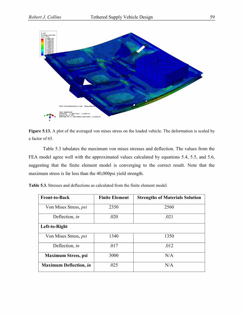
Robert J. Collins Tethered Supply Vehicle Design 59
Figure 5.13. A plot of the averaged von mises stress on the loaded vehicle. The deformation is scaled by
a factor of 65.
Table 5.3 tabulates the maximum von mises stresses and deflection. The values from the
FEA model agree well with the approximated values calculated by equations 5.4, 5.5, and 5.6,
suggesting that the finite element model is converging to the correct result. Note that the
maximum stress is far less than the 40,000psi yield strength.
Table 5.3. Stresses and deflections as calculated from the finite element model.
Front-to-Back Finite Element Strengths of Materials Solution
Von Mises Stress, psi 2350 2560
Deflection, in .020 .021
Left-to-Right
Von Mises Stress, psi 1340 1350
Deflection, in .017 .012
Maximum Stress, psi 3000 N/A
Maximum Deflection, in .025 N/A

Robert J. Collins Tethered Supply Vehicle Design 60
5.6. Vehicle Fabrication
Vehicle fabrication was fairly straight-forward, utilizing .030” thick 6061 aluminum. Part
profiles were cut using a mill (in lieu of a water-jet, or laser cutter) and bent with a brake. Once
the individual parts were fabricated, they were assembled by riveting them together using
AN470A-3-2 solid aluminum rivets. Figure 5.14 shows the vehicle while being fabricated – both
in the component phase and as it’s being assembled together. Figure 5.15 shows the final product
tethered to the ceiling of the Unmanned Systems Lab. In Figure 5.15, all subsystems are present.
The onboard computer and Hokuyo laser range finder are visible. Because testing will focus on
the linear control model presented briefly in this chapter and in chapter 6, the thrust vectoring
servo was not installed.
Figure 5.14. Left – the individual components of the vehicle structure are shown before assembly. Right
– vehicle is in the process of being riveted.
Without batteries, the entire vehicle with all of the systems and wires installed weighed
8.1lb, which is below the 5kg (11.0lb) limit requirement discussed earlier in the chapter. This
reduces the amount of thrust the thrusters must be able to produce to accelerate the vehicle .1g
from the approximate 1lbf discussed earlier. At this point, the vehicle is ready to have the
software uploaded to its onboard computer to tune the control algorithm. The next chapter
focuses on the control of the vehicle.
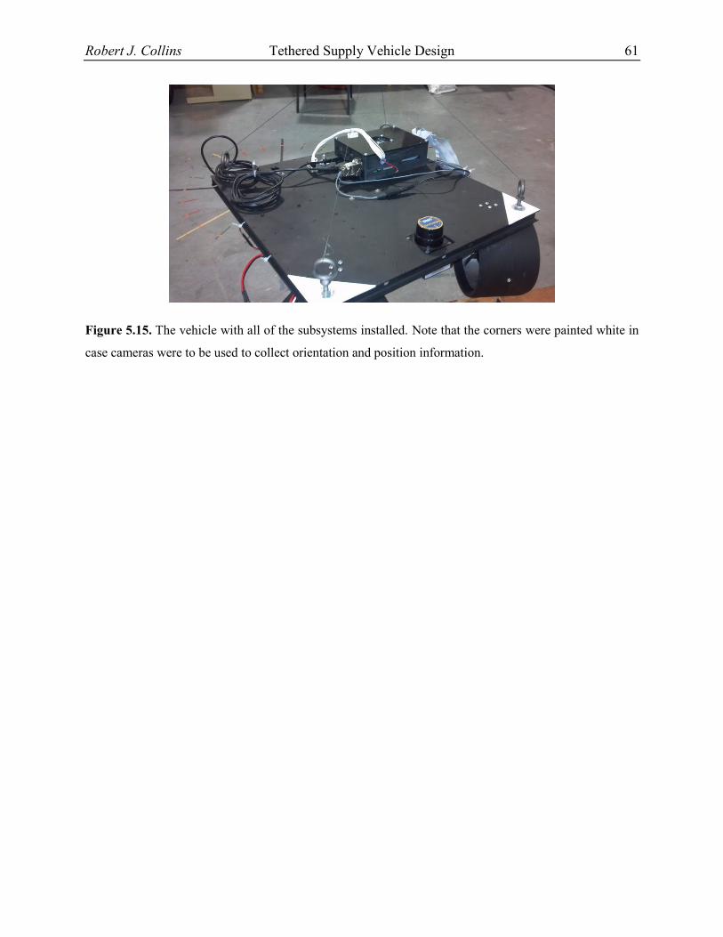
Robert J. Collins Tethered Supply Vehicle Design 61
Figure 5.15. The vehicle with all of the subsystems installed. Note that the corners were painted white in
case cameras were to be used to collect orientation and position information.

Robert J. Collins Controller Design and Implementation 62
Chapter 6 Controller Design and Implementation
Chapter 5 briefly covered the dynamic model and control scheme used to control the
vehicle as it relates to the vehicle’s design. This chapter however will focus more in-depth on the
dynamic model, controller, filtering, etc used to make the vehicle pilotless.
6.1 Spherical Pendulum Dynamics
The tethered vehicle paired with a helicopter resembles dynamics that can be represented
by a spherical pendulum model as it can be described by X, Y, and Z coordinates. To derive the
equations of motion, it was assumed that the base (helicopter) position was fixed, the tether was
massless and rigid, and the payload could be represented by a point mass. Figure 6.1 illustrates a
generic spherical pendulum system.
Figure 6.1. A generic model of a spherical pendulum attached to a fixed point.
Using the labeled parameters in Figure 6.1, the equations of motion were derived by
taking the Lagrangian of the system. The Lagrangian of the system in terms of the angles φ and θ
is shown in equation 6.1.

Robert J. Collins Controller Design and Implementation 63
( ( ) ) ( ) (6.1)
The equations of motion in terms of these angles can be found by applying the Euler-
Lagrange equations. There is more complete derivation of this shown in the appendix showing
this step. From equation 6.1, it is apparent that the Lagrangian is independent of φ. The resultant
equation of motion is shown in equation 6.2.
( ) ( ) ( ) (6.2)
Two immediate problems arise from trying to control a spherical pendulum as governed
by equation 6.2. First and foremost, the equation is nonlinear, presenting a problem for linear
control theory. Second, the equation is in terms of two angular coordinates, θ and φ, both of
which will not be measured. Instead, it is desired to measure the distance from the wall / obstacle
and a corresponding yaw angle (with the Hokuyo laser range finder and Microstrain 3DM-GX2
IMU. This means that the equations of motion should be written in the Cartesian coordinate
system. The linearized equation of motion, in terms of X is presented again below as equations
6.3. A similar equation can be derived for the Y direction; however it is not presented here as it
was not used in the control scheme. In addition, the linearized equation for yaw is presented as
6.4. Note that the nonlinear equations expressed in Cartesian coordinates are not presented. The
derivation is quite long, and is presented in numerous resources such as in [28].
( ) ( ) ( )
(6.3)
(6.4)
The linearized equations of motion presented above are unfortunately valid for only a
small operating range as they omit the difficulties surrounding the true nonlinear equations. For
example, the small angle approximation (sin(x) is approximately equal to x, and cos(x) is
approximately equal to 1) was used to linearize the equations. Large deflections in yaw therefore
cannot be modeled, nor controlled correctly. In addition, the angles φ and θ as defined in Figure
6.1 must remain sufficiently small. As stated earlier, the helicopter is assumed to be stationary.
Recall however that these assumptions and limitations are appropriate for the design range as it
was assumed the helicopter was going to be operated in a quasi-hovered state with small
pendulations.

Robert J. Collins Controller Design and Implementation 64
6.2 Collecting Data and Filtering
Before a controller can be utilized to stabilize the vehicle, the data collected from the
Hokuyo laser range finder and 3DM-GX2 IMU must be fused and filtered. This section of the
chapter discusses the acquisition and processing of the data.
6.2.1 Data Collection
Recall from the previous chapter that data is collected from both the laser ranger finder
and the IMU via USB and serial respectively. Even though both instruments are operating on
relatively fast communication interfaces, they are constrained by their maximum update rates.
These update rates, tabulated in table 6.1, are critically important to the success of any controller
attempting to control a dynamic system. The rates shown in Table 6.1 are ideal as they do not
account for processing / computational time. This is critically important to note for the scanning
laser range finder as the collected data points must be processed first with the wall and window
detection algorithm, which is already computationally intensive for the vehicle’s computer.
Table 6.1. Instrument Update Rates for the primary instruments used onboard the vehicle [22] [24].
Hokuyo URG-04LX 10Hz
3DM-GX2 IMU 250Hz
Accounting for the instrument update rate and all of the processing that must be done, the
vehicle’s instrument update rate is going to be slow. Steps can be taken to combat this however.
It is first noted in Table 6.2 that the dynamic states can theoretically be provided by both the
laser ranger finder and the IMU. Code was written to update the controller with data collected
just from the IMU (as opposed to using the IMU and laser range finder together) when laser
range finder data is unavailable. It’s important to note however that control solely off of the IMU
is normally not done as MEMS (Micro-Electrical-Mechanical) IMU measurements based on the
accelerometer and rate gyros have a bias error and tend to drift if not complemented with another
instrument. Even though the bias error can accumulate quickly, it was hoped that the update rate
of the laser range finder would be sufficient to correct the error and to provide accurate
measurements.
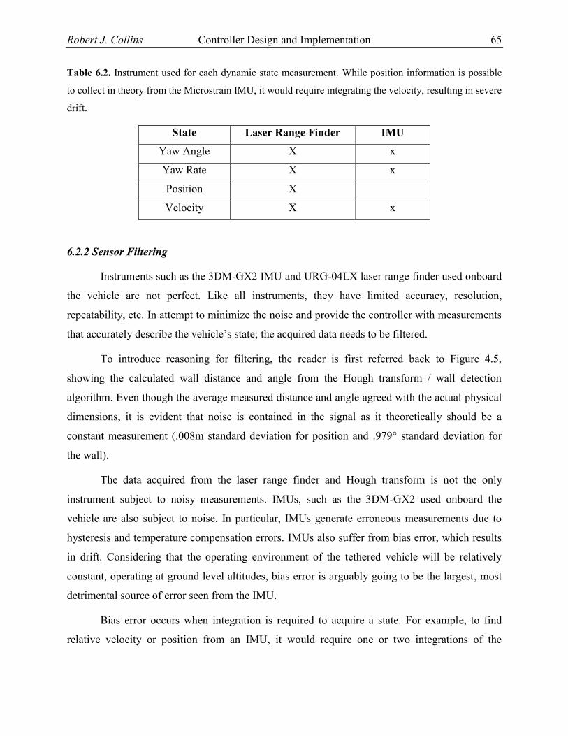
Robert J. Collins Controller Design and Implementation 65
Table 6.2. Instrument used for each dynamic state measurement. While position information is possible
to collect in theory from the Microstrain IMU, it would require integrating the velocity, resulting in severe
drift.
State Laser Range Finder IMU
Yaw Angle X x
Yaw Rate X x
Position X
Velocity X x
6.2.2 Sensor Filtering
Instruments such as the 3DM-GX2 IMU and URG-04LX laser range finder used onboard
the vehicle are not perfect. Like all instruments, they have limited accuracy, resolution,
repeatability, etc. In attempt to minimize the noise and provide the controller with measurements
that accurately describe the vehicle’s state; the acquired data needs to be filtered.
To introduce reasoning for filtering, the reader is first referred back to Figure 4.5,
showing the calculated wall distance and angle from the Hough transform / wall detection
algorithm. Even though the average measured distance and angle agreed with the actual physical
dimensions, it is evident that noise is contained in the signal as it theoretically should be a
constant measurement (.008m standard deviation for position and .979° standard deviation for
the wall).
The data acquired from the laser range finder and Hough transform is not the only
instrument subject to noisy measurements. IMUs, such as the 3DM-GX2 used onboard the
vehicle are also subject to noise. In particular, IMUs generate erroneous measurements due to
hysteresis and temperature compensation errors. IMUs also suffer from bias error, which results
in drift. Considering that the operating environment of the tethered vehicle will be relatively
constant, operating at ground level altitudes, bias error is arguably going to be the largest, most
detrimental source of error seen from the IMU.
Bias error occurs when integration is required to acquire a state. For example, to find
relative velocity or position from an IMU, it would require one or two integrations of the
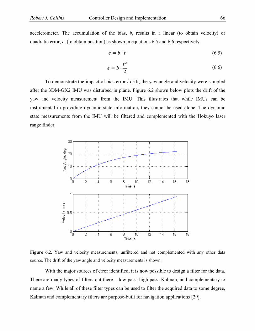
Robert J. Collins Controller Design and Implementation 66
accelerometer. The accumulation of the bias, b, results in a linear (to obtain velocity) or
quadratic error, e, (to obtain position) as shown in equations 6.5 and 6.6 respectively.
(6.5)
(6.6)
To demonstrate the impact of bias error / drift, the yaw angle and velocity were sampled
after the 3DM-GX2 IMU was disturbed in plane. Figure 6.2 shown below plots the drift of the
yaw and velocity measurement from the IMU. This illustrates that while IMUs can be
instrumental in providing dynamic state information, they cannot be used alone. The dynamic
state measurements from the IMU will be filtered and complemented with the Hokuyo laser
range finder.
Figure 6.2. Yaw and velocity measurements, unfiltered and not complemented with any other data
source. The drift of the yaw angle and velocity measurements is shown.
With the major sources of error identified, it is now possible to design a filter for the data.
There are many types of filters out there – low pass, high pass, Kalman, and complementary to
name a few. While all of these filter types can be used to filter the acquired data to some degree,
Kalman and complementary filters are purpose-built for navigation applications [29].
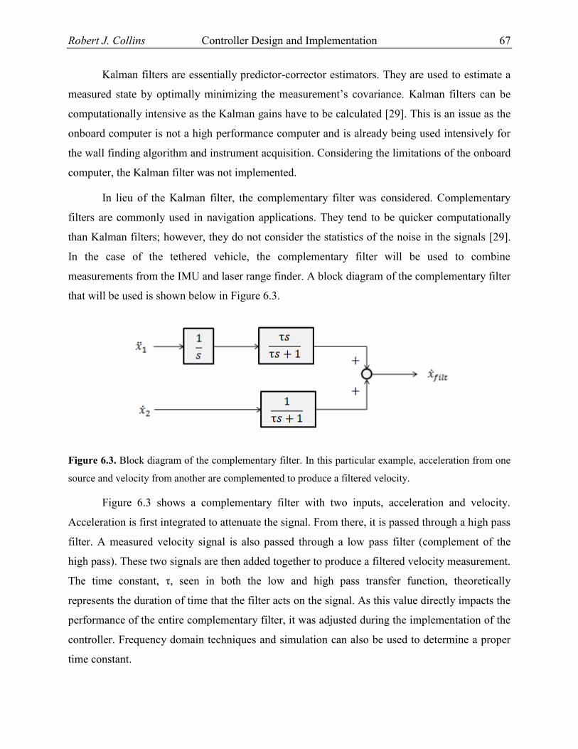
Robert J. Collins Controller Design and Implementation 67
Kalman filters are essentially predictor-corrector estimators. They are used to estimate a
measured state by optimally minimizing the measurement’s covariance. Kalman filters can be
computationally intensive as the Kalman gains have to be calculated [29]. This is an issue as the
onboard computer is not a high performance computer and is already being used intensively for
the wall finding algorithm and instrument acquisition. Considering the limitations of the onboard
computer, the Kalman filter was not implemented.
In lieu of the Kalman filter, the complementary filter was considered. Complementary
filters are commonly used in navigation applications. They tend to be quicker computationally
than Kalman filters; however, they do not consider the statistics of the noise in the signals [29].
In the case of the tethered vehicle, the complementary filter will be used to combine
measurements from the IMU and laser range finder. A block diagram of the complementary filter
that will be used is shown below in Figure 6.3.
Figure 6.3. Block diagram of the complementary filter. In this particular example, acceleration from one
source and velocity from another are complemented to produce a filtered velocity.
Figure 6.3 shows a complementary filter with two inputs, acceleration and velocity.
Acceleration is first integrated to attenuate the signal. From there, it is passed through a high pass
filter. A measured velocity signal is also passed through a low pass filter (complement of the
high pass). These two signals are then added together to produce a filtered velocity measurement.
The time constant, τ, seen in both the low and high pass transfer function, theoretically
represents the duration of time that the filter acts on the signal. As this value directly impacts the
performance of the entire complementary filter, it was adjusted during the implementation of the
controller. Frequency domain techniques and simulation can also be used to determine a proper
time constant.

Robert J. Collins Controller Design and Implementation 68
To illustrate the usefulness of the complementary filter, the angle from the wall is plotted
below in Figure 6.4. In the complementary filter, the laser range finder output was
complemented with the IMU’s angular velocity output. Figure 6.4 plots the calculated wall angle
(in blue) from the Hough transform / laser range finder and the total state output as calculated
from the complementary filter (in red).
Figure 6.4. The perpendicular angle from the wall filtered and unfiltered. The perpendicular angle from
the wall from the laser range finder is displayed in blue. The complementary filtered angle is shown in
red.
The blue (original as calculated by the laser range finder) plot shown in Figure 6.4 is
quite noisy compared to the filtered (red) plot. Considering that the tethered vehicle is a slow
moving system, it is unlikely it would ever see angular rates of change as indicated by the
original laser range finder output. If the vehicle was controlled off of the unfiltered input, it is
likely it would oscillate, if not diverge. Figure 6.5 plots the position from the wall as collected
from the laser range finder and complemented with the IMU output. While the noise associated
with position is much less, the filter nevertheless attenuates the signal.

Robert J. Collins Controller Design and Implementation 69
Figure 6.5. The perpendicular distance filtered and unfiltered. Perpendicular distance from the wall from
the laser range finder is shown in blue, while the filtered is shown in red.
It’s important to note that the complementary filter time constant, τ, is a function of the
sampling time between intervals, dt. With a real time operating system, it’s possible to control
the sampling intervals, meaning the time constant will be constant. The vehicle’s onboard
computer is not a real time operating system however. As such, sampling times from iteration to
iteration may be different, which may degrade the performance of the filter if severe enough.
6.3 Controller Design
This section of the chapter expands upon the controller design discussed in Chapter 5.
The results of testing the implemented discrete controller are also compared to simulations and
discussed.
6.3.1 Multiple Input Multiple Output Control
Multiple-input multiple-output control can be achieved in many different ways. In the
linear control world, this is commonly done by a full state feedback controller utilizing state-

Robert J. Collins Controller Design and Implementation 70
space equations. Optimal methods also exist for linear controllers, such as the linear quadratic
regulator. The controller designed for the tethered vehicle is a full state feedback controller; of
which iterative pole placement techniques were used.
Before a controller can be designed, a state space representation of the dynamic system
must be derived. Equation 6.8, reprinted from earlier in section 6.1 and also in Chapter 5, is
shown below and represents the state space representation of the system. This system will be
controlled using the linear control law shown in equation 6.9. Using equation 6.8, the controller
(6.9) will be able to control yaw angle, yaw angle rate, position from the wall, and velocity to the
wall. Recall that sway parallel to the wall and the motor / shrouded propeller dynamics are not
accounted for in these equations. Equation 6.8 utilizes the assumptions discussed in section 6.1.
In particular, small oscillations and yaw of the payload is necessary for equation 6.8 to be valid.
(6.7)
[
]
[
]
[
]
[
( ( )
) (
( )
) (
( )
) (
( )
)]
[
] (6.8)
The next step in designing a linear full state feedback controller is to determine
controllability. By calculating the controllability matrix, controllability of the system can be
determined. This is done by subtracting the rank of the controllability matrix from the maximum
length of the A matrix. Executing this calculation reveals that for the given physical parameters
of the system, no uncontrollable states exist. The system should be controllable given proper pole
placement.
(6.9)
Once controllability was determined, the open loop system was turned into a closed loop
system by placing a feedback loop with gain matrix K in the loop and utilizing the control law in
equation 6.9. A Simulink schematic is shown in Figure 6.6. Pole placement techniques were used
to calculate the gain matrix K. Considering pole placement determines the eigenvalues of the A-
BK matrix (the closed loop system), this is a critical step. Placing poles therefore directly
influences the dynamics of the system. Incorrectly placing poles can result in an unstable system.
Pole placement will also influence the system’s response (speed, oscillation, etc).

Robert J. Collins Controller Design and Implementation 71
Figure 6.6. Original Simulink model used to design the full state feedback controller.
Similar to the method explained in Chapter 5, pole placement was done iteratively by a
MATLAB script and Simulink model. Poles were changed for the given design parameters with
the goal of minimizing settling time. In addition, thruster output was examined to make sure the
thrusters were not saturating during operation. Several poles (and therefore gain matrices) were
selected and tested with mixed success (this process will be explained later).
It’s important to note that the full state feedback controller designed to control the vehicle
was designed in continuous time. This is significant as the controller will be executed on a
computer, where the state and actuation update rates will be discrete. Seeing as most
implementations are discrete, this isn’t necessarily an unknown practice. Implementing a
controller designed in continuous time will cause the eigenvalues of the system (and therefore
cause the dynamic response to change) when implemented on a discrete system.
The controller was simulated in continuous time and implemented discretely (using a
digital computer to execute it). Both results indicated that the system should remain stable. The
system responses of the continuous and discrete implementations are shown in Figure 6.7. Figure
6.8 plots the shrouded propeller output for the continuous and discrete controllers. Note that the
red plotted line is the discrete controller.
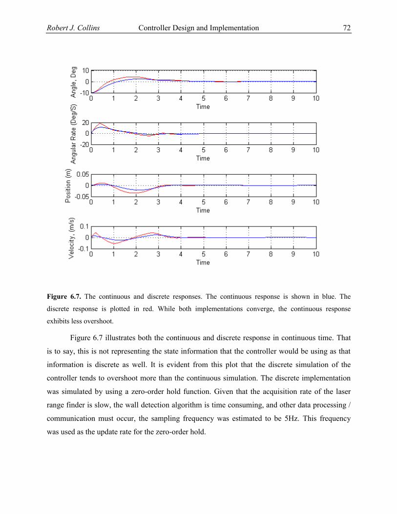
Robert J. Collins Controller Design and Implementation 72
Figure 6.7. The continuous and discrete responses. The continuous response is shown in blue. The
discrete response is plotted in red. While both implementations converge, the continuous response
exhibits less overshoot.
Figure 6.7 illustrates both the continuous and discrete response in continuous time. That
is to say, this is not representing the state information that the controller would be using as that
information is discrete as well. It is evident from this plot that the discrete simulation of the
controller tends to overshoot more than the continuous simulation. The discrete implementation
was simulated by using a zero-order hold function. Given that the acquisition rate of the laser
range finder is slow, the wall detection algorithm is time consuming, and other data processing /
communication must occur, the sampling frequency was estimated to be 5Hz. This frequency
was used as the update rate for the zero-order hold.

Robert J. Collins Controller Design and Implementation 73
Figure 6.8. Simulated actuator / thruster output for the continuous and discrete implementations of the
controller. The discrete controller is shown in red.
The controller was designed for the physical parameters shown in Table 6.3. These
values were predicted from computer generated solid models and verified with measurements.
These are important to note, as while the controller will exhibit some robustness, a significant
deviation from these physical values could cause divergence. In an actual implementation of the
vehicle, these parameters could change significantly depending on the payload and tether length.
Table 6.3. Physical parameters used in designing the linear full state feedback controller. The controller
was tested onboard a vehicle with these physical parameters
Parameter Value
Pendulum Length, m 3.8
Mass, kg 4.4
Moment of Inertia, kgm2 .121
Thrust Saturation, N 3.1
6.3.2 Modeling Deficiencies
Despite simulating the controller in discrete time, several modeling deficiencies exist. In
addition to the linearized dynamics the controller must use for a nonlinear problem, the
following deficiencies exist:

Robert J. Collins Controller Design and Implementation 74
The thrusters / shrouded propellers have dynamics of their own that are not accounted
for. In the model presented above, the controller is assuming an instantaneous response of
the shrouded propellers. In reality, the motors have a finite acceleration and therefore
need time to spin up to speed. Likewise, the shrouded propellers’ angular velocity cannot
be reduced instantaneously. These deficiencies are arguably the most important. In
addition, the dynamic effects associated with the shrouded propeller are not characterized
either (static thrust was characterized only at steady state).
Gyroscopic effects of the shrouded propellers are not accounted for. If the propellers are
spinning while the vehicle is rotating, forces will be generated due to the angular
conservation of momentum. These forces will vary with respect to the angular velocities
of the propellers and the vehicle.
Aside from the simulated 5Hz zero-order hold, the software acquisition and output is not
accounted for (ex communication between instruments, microcontroller, etc). Seeing as
the onboard computer is running Microsoft Windows with NI’s LabVIEW, it is possible
for the iteration / update rates of the controlling and acquisition loops to be variable as
low level timing control is not possible. It is for these reasons that the 5Hz rate may not
be realistic at times.
Long tether dynamic are not accounted for. The model assumes that the tether is always
in tension and aside from the joints, not flexible. In reality, a tether is unable to resist any
appreciable moment. Depending on the length of the tether, aerodynamic drag due to
translation, wind, etc, could influence the dynamics.
6.4 Controller Implementation
After designing the controller and simulating it in MATLAB, it was coded in LabVIEW
and installed on the vehicle’s onboard computer. Many implementations were attempted by
varying the matrix K and saturation limits. The response of each implementation was compared.
This section of the chapter discusses the testing of the vehicle controller. In addition, the several
issues were discovered during the testing of the controller are discussed.
6.4.1 Verifying the Controller
Many experiments were run to verify the operation of the designed controller. In
particular, the controller was tested to make sure the vehicle was stable and to verify its response

Robert J. Collins Controller Design and Implementation 75
to small disturbances. The vehicle was tested using DOW residential sheathing to simulate walls
/ windows. To simulate a tether, the vehicle was suspended from the ceiling of the Unmanned
Systems Lab using a 3.8m length 80lb test line.
Many implementations of different gain matrices K and actuator saturation limits were
tested with the vehicle. Even though simulations indicated stability, some implementations were
not stable for all time. In addition, it was found that the vehicle entered instability when the
position state deviated from zero. This is most likely due to the fact that the vehicle’s controller
did not control yaw very well. A plot of the yaw state as collected is shown in Figure 6.9.
Compared to the simulations for the same initial conditions shown also in Figure 6.9, the actual
implementation does not agree well as the actual controller does not settle. If the vehicle was
trying to control position as well, this extreme oscillation would violate the small angle
approximation and cause the vehicle to go unstable.
Figure 6.9. Comparison of actual yaw data to simulated data. Actual response is plotted as blue, while the
discrete response is shown in red. The implemented controller does not settle.
The behavior shown in Figure 6.9 was typical of all stable controllers implemented on the
vehicle. Physical parameters such as the mass, moment arms of the shrouds, center of gravity
(and rotation), and moment of inertia of the vehicle were measured and verified through

Robert J. Collins Controller Design and Implementation 76
software. The shrouded propeller saturation limits were also adjusted multiple times. In these
trials, it was discovered that 25% of the maximum producible thrust was the maximum allowable
saturation limit before the vehicle’s motion became divergent. The “thrust vectoring” shroud was
placed in multiple orientations, with no significant improvement. Despite these efforts, the
controller response did not noticeably improve. Several cases were run with the wires suspended
from the edge of the vehicle (used to power the vehicle). In these cases, the vehicle eventually
settled (attributed to the light damping / restoring force of the wires).
The failure of the controller to adequately control yaw and distance from the wall is
attributed to the model deficiencies discussed previously in this chapter (section 6.3.2). In
particular, it is thought that deriving a model that can account for more of the dynamics would be
beneficial. This includes modeling of the shrouded propellers and their respective electronic
speed controllers, the gyroscopic forces, and perhaps using more representative nonlinear
equations. A linear model based on pole placement or optimization techniques such as a linear
quadratic regulator may be used with some success if the shrouded propeller dynamics are more
appropriately accounted for.
A simulation was recreated in MATLAB Simulink using the same linear controller in
attempt to match the experimental data. This new model included the use of time constants in
attempt to simulate the inertia and response of the shrouded propellers. The simulated plot as
compared to the actual data is shown below in Figure 6.10. The period and amplitude of the
simulation are roughly equivalent to the actual collected data. Several sources of error include
the variable sampling increment and the simulation of collected data with noise and filtering. It’s
important to note though that the use of a time constant to represent the shrouded propellers can
be deceiving. In essence, all of the dynamic deficiencies are being lumped into the time constant.
While it is likely that the shrouded propellers do have a significant lag as discussed earlier, it is
difficult to ascertain the relative magnitude and contribution of each deficiency.

Robert J. Collins Controller Design and Implementation 77
Figure 6.10. Comparison of actual yaw data to corrected simulated data. Time constants are included to
represent the actual dynamics and control. The implemented (blue) and simulated controller (red) do not
settle.
6.5 Momentum Actuation and Control
In addition to using the shrouded propellers as actuators, yaw control by the use of a
momentum-exchange system was investigated, simulated, and tested. This was primarily done as
the controller developed for the shrouded propellers exhibited little control authority. In addition,
it was of interest if actuation by another method with the same hardware and sensors could
provide better authority. Momentum control was achieved by the use of a reaction wheel. In
general, reaction wheels find their use in space vehicle applications such as satellites. They are
generally used as part of a broader attitude control system, which may feature several reaction
wheels, thrusters, etc. Reaction wheels in these systems are often used to compensate for small
disturbances such as radiation pressure. Using a motor or other device to spin the wheel,
momentum can be exchanged between the vehicle and the actuator and the orientation of the
vehicle can be preserved [30].

Robert J. Collins Controller Design and Implementation 78
Reaction wheels do have their disadvantages. In particular, due to conservation of angular
momentum and the physical limitations of the motor / device to actuate the wheel, the wheel may
saturate. That is to say, the maximum speed of the reaction wheel may be reached before the
disturbance is compensated for.
The reaction wheel as an actuation method was implemented onboard the tethered vehicle
for several different reasons. First, the dynamic model of a single reaction wheel to control yaw
is relatively simple and can describe the dynamics more completely than the model used for the
shrouded propellers. System parameters such as the motor constants, moments of inertia, etc are
respectively published by manufacturers and can be designed for. In addition, by using the more
complete reaction wheel dynamic model, it may be possible to evaluate if system deficiencies
such as the slow update rates still act as a severe detriment to the controller.
6.5.1 Reaction Wheel Design
The reaction wheel actuation system was designed to be small enough to fit onboard the
vehicle in the payload area and to possess enough actuation authority to yaw the vehicle. First, a
motor, motor controller / driver, and gearbox were selected. These were selected based on
simulations conducted in MATLAB Simulink to determine the necessary torque to actuate the
vehicle based on a given initial condition and the maximum rotational velocity. A Maxon EC-
max30 brushless DC motor with a GP32 4.8:1 gearhead was selected to provide actuation to the
reaction wheel. To drive the wheel, a Maxon DEC 50/5 motor controller was selected. The DEC
50/5 is capable of speed and current control modes by the use of a 0-5V analog pin. In addition,
the 50/5 driver is able to reverse direction and brake the motor (although uncontrolled) by
shorting the coils. Finally, a National Instruments myDAQ was used to provide the 0-5V and
digital pins required by the DEC 50/5. Figure 6.11 shows the system layout for the reaction
wheel.
Figure 6.11. The reaction wheel system layout.
Several reaction wheels were designed and machined out of 6061 aluminum into a solid
circular disc. The wheel and motor were mounted at the vehicle’s center of mass. The physical

Robert J. Collins Controller Design and Implementation 79
parameters of the system as implemented are shown in Table 6.4. It’s important to note that the
machined wheel must be concentric and balanced, especially if the vehicle is expected to
counteract any disturbance.
Table 6.4. Physical parameters of the reaction wheel.
Parameter Value
Wheel Moment of Inertia, kg-m2 .0028
Motor Rotor Inertia, g-cm2 21.9
Motor Torque Constant, Nm/A .0243
Motor and Gearhead No-Load Max RPM 1940
Figure 6.12 is a photograph of the implemented system. The reaction wheel consumed
most of the usable payload area of the vehicle. An actual practical implementation would most
likely have to include a wheel below the payload area to ensure the vehicle is still useful.
Figure 6.12. The reaction wheel implemented onboard the vehicle.
6.5.2 Reaction Wheel Dynamic Model
As stated earlier, the reaction wheel dynamic model is simple consisting of mostly known
parameters. The model presented in equations 6.10 (rewritten as 6.11 in terms of the wheel
moment of inertia and acceleration) was derived using a torque balance. The torque, T, required
to actuate the vehicle can be written in terms of the moment of inertia of the wheel and angular
acceleration. Torque can also be expressed in terms of current and the torque-current constant of

Robert J. Collins Controller Design and Implementation 80
the motor. These relationships were used to develop a linear full state feedback controller,
controlling angle and angular rate of the vehicle.
(6.10)
(6.11)
The DEC 50/5 will be used to control current delivered to the motor. This is critical
because while many of the system parameters are known in this case, the characteristics of the
DEC 50/5 motor driver / controller are not known. While the 0-5V input to output current
relationship can be measured, the actual response, braking, slowing down (the motor will spin
down in an uncontrolled fashion), etc can be difficult to characterize and incorporate into control
dynamics. In addition, the gears in the gearhead will have some sort of backlash that can become
evident, especially if the wheel has to change direction or slow down substantially (during
testing, the backlash was audible during direction change). Nevertheless, equation 6.10 with the
system parameters discussed in this chapter was formed into a state space equation which was
used to implement a linear full state feedback controller.
6.5.3 Controller Implementation
As stated previously, a linear full state feedback controller was implemented to control
the vehicle via actuating the reaction wheel. It’s important to note here that during testing that
the motor was constrained through limits imposed in software. This was done to prevent the
motor from damaging the DEC 50/5 should the software controller want to brake / change
directions of the motor. This limited the amplitude of the disturbances that could be introduced
into the system.
The controller was first evaluated in its steady state performance. This was done ensuring
the vehicle was first parallel with the wall before the controller was enabled. Once the controller
was enabled, the yaw was collected and plotted in Figure 6.13. Note how the vehicle still
oscillates, although at a much smaller amplitude as before with the shrouded propellers (about 2
degrees from the mean 0). This oscillation is most likely due to the slow update rates (which
have not changed from the shrouded propeller actuation) and the model deficiencies.

Robert J. Collins Controller Design and Implementation 81
Figure 6.13. Yaw performance using the reaction wheel at steady state.
It’s important to note that the reaction wheel controller, while written in LabVIEW, was
not implemented on the PC104. The controller was implemented on a computer with an Intel
Core2 Duo clocked at 2.54GHz with 4.00GB of RAM, which is substantially faster than the
PC104. While computation time should decrease with this setup, the acquisition limitations of
the instruments (laser range finder and IMU) should stay the same. The computer running the
controller was not equipped onboard the vehicle. This required several wires to be connected to
the vehicle, which arguably provided some amount of damping and restoring torque.
Several tests were conducted by setting the vehicle to an initial condition. In these tests,
the wheel was able to turn the vehicle to have a 0 degree angle with the wall. The results of such
a test are shown in Figure 6.14.

Robert J. Collins Controller Design and Implementation 82
Figure 6.14. Yaw performance using the reaction wheel with an initial condition of approximately 15
degrees.
As Figure 6.14 illustrates, the vehicle was able to be turned successfully to the proper
orientation. Notice the vehicle still oscillates about the zero set point. This again is due to
probably the slow sampling rate and model deficiencies. Recall that the motor will spin freely
down in an uncontrolled manner. The lack of control is probably one of the single biggest
deficiencies of the model and most likely contributes the most to the oscillatory response. The
system response to other initial conditions was similar to that shown in Figure 6.14, possessing
the oscillatory behavior about 0 degrees. This was true so long as the Hokuyo laser range finder
was able to see a wall.
Even though the controller seemed to perform better than the controller using the
shrouded propellers, several practical considerations remain. First and foremost is the actuation
authority of the reaction wheel. A long duration or high amplitude disturbance torque can
saturate the reaction wheel rendering it useless. Second, the reaction wheel usually must be
designed to have a relatively high moment of inertia. This generally involves using a

Robert J. Collins Controller Design and Implementation 83
combination of a high density material and a large diameter wheel. These two traits contrast the
requirements of the vehicle to be light and to be able to support some sort of payload. The wheel
will not only lower the useful weight of the tethered vehicle but also use area and volume that
could otherwise be used to carry a useful load.

Robert J. Collins Conclusion and Recommendations 84
Chapter 7 Conclusion and Recommendations
This thesis presented the research and design methodology used in the development of
the helicopter slung actuated vehicle. The completed tasks and a discussion of recommended
changes to continue onward with this research are presented in this final chapter.
7.1 Summary of Work
The overall design requirements and project motivation / applications are discussed in the
first chapter. These design requirements with the consideration of the project motivation were
used to develop a helicopter slung vehicle for the purpose of precision placement of payloads.
The overall vehicle requirements imposed requirements on the vehicle’s subsystems.
The vehicle developed in this thesis was unique not only in terms of application, but also
in the fact that it required multiple, very different systems to be developed, tested, and
implemented. This included the development of the propulsion system, the wall and window
detection system, the controller, and the system architecture / mechanical design of the vehicle
itself. Each system was split into its own separate chapter, covering the design requirements of
that and the resultant design / implementation of each individual system.
The propulsion system was the first system to be presented in this thesis. Utilizing the
vehicle design requirements, design requirements specific to propulsion were developed and
presented. In particular, a system that was relatively quiet and could produce 1.0lbf in the
direction perpendicular to the wall was desired. After briefly examining multiple propulsion
mechanisms / machinery, it was decided to utilize shrouded propellers. Shrouded propellers were
researched to develop a set of more specific design requirements. From these requirements, a
shrouded propeller that had a nominal 5.0” inlet diameter and had a 4.0” chord length was
designed. To increase thrust output, a diffuser was designed, causing the shroud to have an area
ratio of 1.25.
Initially, the shrouded propeller was manufactured completely by an FDM rapid
prototyping machine utilizing a machined down remote control aircraft propeller. The shrouded
propeller was characterized in a series of static thrust tests. Power consumption, thrust, and thrust
vs pulse width of the electronic speed control were determined. Unfortunately however, the
prototype shroud had several deficiencies, the most important being an eccentric shroud.
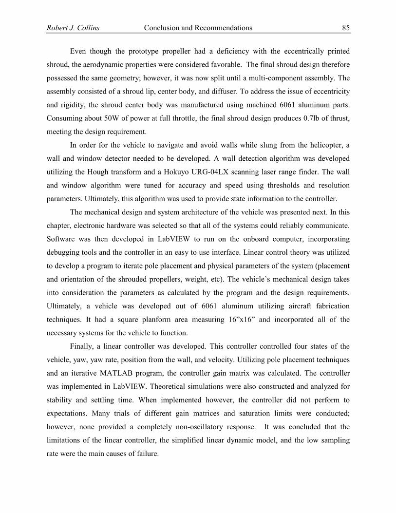
Robert J. Collins Conclusion and Recommendations 85
Even though the prototype propeller had a deficiency with the eccentrically printed
shroud, the aerodynamic properties were considered favorable. The final shroud design therefore
possessed the same geometry; however, it was now split until a multi-component assembly. The
assembly consisted of a shroud lip, center body, and diffuser. To address the issue of eccentricity
and rigidity, the shroud center body was manufactured using machined 6061 aluminum parts.
Consuming about 50W of power at full throttle, the final shroud design produces 0.7lb of thrust,
meeting the design requirement.
In order for the vehicle to navigate and avoid walls while slung from the helicopter, a
wall and window detector needed to be developed. A wall detection algorithm was developed
utilizing the Hough transform and a Hokuyo URG-04LX scanning laser range finder. The wall
and window algorithm were tuned for accuracy and speed using thresholds and resolution
parameters. Ultimately, this algorithm was used to provide state information to the controller.
The mechanical design and system architecture of the vehicle was presented next. In this
chapter, electronic hardware was selected so that all of the systems could reliably communicate.
Software was then developed in LabVIEW to run on the onboard computer, incorporating
debugging tools and the controller in an easy to use interface. Linear control theory was utilized
to develop a program to iterate pole placement and physical parameters of the system (placement
and orientation of the shrouded propellers, weight, etc). The vehicle’s mechanical design takes
into consideration the parameters as calculated by the program and the design requirements.
Ultimately, a vehicle was developed out of 6061 aluminum utilizing aircraft fabrication
techniques. It had a square planform area measuring 16”x16” and incorporated all of the
necessary systems for the vehicle to function.
Finally, a linear controller was developed. This controller controlled four states of the
vehicle, yaw, yaw rate, position from the wall, and velocity. Utilizing pole placement techniques
and an iterative MATLAB program, the controller gain matrix was calculated. The controller
was implemented in LabVIEW. Theoretical simulations were also constructed and analyzed for
stability and settling time. When implemented however, the controller did not perform to
expectations. Many trials of different gain matrices and saturation limits were conducted;
however, none provided a completely non-oscillatory response. It was concluded that the
limitations of the linear controller, the simplified linear dynamic model, and the low sampling
rate were the main causes of failure.

Robert J. Collins Conclusion and Recommendations 86
7.2 Suggestions for Future Work
This thesis presents a good foundation for an actuated tethered vehicle. Even so, there are
many improvements one could make should the research be continued. Deficiencies exist at a
system and vehicle level that should be corrected to increase reliability. This section of the
chapter identifies deficiencies that should be corrected in the future.
While the shrouded propellers satisfy the design requirements, they can be improved a
number of different ways. For example, the propellers used in the shrouded propeller are
commercially available propellers for remote control aircraft that were machined to fit inside the
shroud. Propellers can potentially be fabricated using injection molding techniques to better suit
the application. For example, the solidity ratio, chord length, number of blades, angle of
incidence, etc, can all be manipulated and optimized for the operating conditions of the shroud.
In addition to propellers, the shrouds can be redesigned to save weight and space. This
can be achieved principally by addressing the shrouded propellers length. Recall that the shrouds
were designed to be rather long to assist the diffuser. However, with experimental data showing
the diffuser is only causing modest gains in thrust, the diffuser can probably be shortened.
Decreasing the chord length of the shroud will reduce viscous drag, possibly allowing for an
increased thrust output. Nevertheless, shortening the chord length will decrease the weight of the
vehicle.
Since the shrouded propellers are the actuators the controller is using to orient the
vehicle, their dynamics are important. In this thesis, the characterization of the thrust and pulse
width signal delivered to the electronic speed controller was used in the controller to determine
the thrust output. In actuality, the shrouded propeller has dynamics of its own as the motor has a
finite acceleration. Modeling the shrouded propellers accurately would likely help in the control
of the vehicle.
The wall and window detector seems to work accurately and produce repeatable results.
However, the speed of the detector can probably be increased using a probabilistic Hough
transform. In any case, the Hokuyo URG-04LX is not sufficient for acquiring the data. With scan
rates of 100ms, the URG-04LX inherently limits the update speed of the vehicle. For a system
that needs to have a controller onboard to perform correctly, this limitation placed on the update

Robert J. Collins Conclusion and Recommendations 87
rate is certainly not ideal. To correct this, another instrument (or multiple instruments) should
probably be used to obtain faster acquisition rates.
In addition to the scanning laser range finder, acquisition and update rates are influenced
by the onboard PC104 computer. The PC104, used in many embedded applications, is not
necessarily the best computational platform to use for this application. Equipped with just an
Intel Atom processor and 1.0GB of RAM, the computer is far from state-of-the-art. In addition to
this, the onboard computer was running Microsoft Windows and LabVIEW, both of which can
be resource demanding. This combination of software left a lot to be desired as well – as
minimum timing control was available at this level. To correct this in the future, a computational
platform that has a real time processor should be investigated. FPGAs, National Instruments’
RIO, and various other platforms exist that could provide more computational power and access
to the lower level hardware. If a platform is selected that has digital GPIO ports available, the
ATmega1280 microcontroller used in the system architecture could be eliminated in its entirety.
Even though the simulated controller did well, the actual implemented controller left a lot
to be desired. The controller is undoubtedly influenced by the update rate issue discussed
previously. In addition, highly nonlinear system dynamics were linearized. This is inconsistent
with the actual dynamics and is somewhat responsible for poor controller performance,
especially when the system experiences a large perturbation, or needs to control position while
yawing. To correct this issue, a more advanced modern controller may need to be implemented.
While an optimal linear controller, such as the linear quadratic regulator, can be used with
probably a little more success on a faster system that modeled more of the dynamics (ex thruster
dynamics), it may be worth it to jump straight to a controller that can account for the nonlinear
dynamics. In addition, this system will be experiencing large disturbance forces as well from the
rotor blades, wind / wind gusts, etc – all of which may cause a linear controller to diverge.
While a tether ideally doesn’t collapse and can be modeled as a rigid link, this may not be
adequately representative enough of tether dynamics. Future work therefore may include
investigating scenarios at which the vehicle is deployed using a very long tether. For example,
the dynamics of a long tether may be susceptible to the wind and gust like disturbances. These
disturbances could cause the vehicle / tethered payload to deviate from its orientation and
position.

Robert J. Collins Bibliography 88
Bibliography
[1] Department of the Air Force, Airdrop of Supplies and Equipment: Rigging Airdrop
Platforms TO13C7-1-5, Washington, DC: Headquarters, 2001.
[2] Lockheed Martin, "K-MAX Delivers for U.S. Marines," 31 January 2012. [Online].
Available: http://www.lockheedmartin.com/us/ms2/features/120131-k-max-delivers-for-u-
s-marines.html. [Accessed 19 February 2012].
[3] J. Vaughan, A. Yano and W. Singhose, "Comparison of robust input shapers," Journal of
Sound and Vibration, vol. 315, no. 4-5, pp. 797-815, 2008.
[4] W. Singhose, J. Lawrence, K. Sorensen and D. Kim, "Applications and Educational Use of
Crane Oscillation Control," FME Transactions, vol. 34, no. 4, pp. 175-183, 2006.
[5] J. Lawrence and W. Singhose, "Command Shaping Slewing Motions for Tower Cranes,"
Journal of Vibrations and Acoustics, vol. 132, no. 1, 011002, 2010.
[6] R. A. Stuckey, "Mathematical Modelling of Helicopter Slung-Load Systems," DSTO
Aeronatuical and Maritime Research Laboratory, Victoria, Australia, 2002.
[7] J. E. May, "Tethered Payload Control from an Autonomous Helicopter," Virginia
Polytechnic Institute and State University, 2010.
[8] Input Shaping Lab @ Georgia Tech, "Flying Crane Research," 29 May 2007. [Online].
Available: http://singhose.marc.gatech.edu/FlyingCrane/index.html. [Accessed 21 February
2012].
[9] S.-R. Oh, J.-C. Ryu and S. K. Agrawal, "Dynamics and Control of a Helicopter Carrying A
Payload Using A Cable-Suspended Robot," University of Delaware, Newark, 2005.
[10] W. Kruger, "On Wind Tunnel Tests and Computations Concerning the Problem of
Shrouded Propellers," National Advisory Committee for Aeronautics, Washington, 1949.
[11] R. J. Platt, "Static Tests of a Shrouded and an Unshrouded Propeller," National Advisory
Committee for Aeronautics, Washington, 1948.
[12] H. H. Hubbard, "Sound Measurements for Five Shrouded Propellers at Static Conditions,"
National Advisory Committee for Aeronautics, Washington, 1950.
[13] D. M. Black, H. S. Wainauski and C. Rohrbach, "Shrouded Propllers - A Comprehensive
Performance Study," American Inst of Aeronautics and Astronautics, Philadelphia, 1968.
[14] R. O. Duda and P. E. Hart, "Use of the Hough Transform to Detect Lines and Curves in
Pictures," Artificial Intelligence Center, Menlo Park, 1971.
[15] C. Galambos, J. Matas and J. Kittler, "Progressive Probabilistic Hough Transform for line
detection," in Computer Vision and Pattern Recognition, 1999. IEEE Computer Society
Conference on., Fort Collins, 1999.
[16] P. Kultanen, L. Xu and E. Oja, "Randomized Hough Transform (RHT)," in Pattern
Recognition, 1990. Proceedings., 10th International Conference on, 1990.
[17] K. D. Korkan, G. M. Gregorek and D. C. Mikkelson, "A Theoretical and Experimental
Investigation of Propeller Performance Methodologies," in AIAA/ASME/SAE 16th Joint
Propulsion Conference, Hartford, 1980.
[18] A. Raspet, "The Ducted Propeller for STOL Airplanes 60-AV-11," in ASME Aviation

Robert J. Collins Bibliography 89
Conference, Dallas, 1960.
[19] A. Akturk and C. Camci, "Tip Clearance Investigation of a Ducted Fan Used in VTOL
UAVS," in ASME Turbo Expo Turbine Technical Conference, Vancouver, 2011.
[20] R. J. Weir, "Ducted Propeller Design and Analysis," Sandia National Laboratories,
Albuquerque, 1987.
[21] R. J. Weir, "Aerodynamic Design Considerations for a Free-Flying Ducted Propeller," in
AIAA Atmospheric Flight Mechanics Conference, Minneapolis, 1988.
[22] Hokuyo, "Hokoyo Laser Range Finder URG-04LX Specifications," [Online]. Available:
http://www.hokuyo-aut.jp/02sensor/07scanner/urg_04lx.html. [Accessed 20 January 2012].
[23] Embedded Solutions, "ADLS15PC," [Online]. Available: http://www.adl-
usa.com/products/cpu/datasheets/ADLS15PC.pdf. [Accessed 25 January 2012].
[24] MicroStrain, "3DM-GX2 Technical Product Overview," 13 July 2008. [Online]. Available:
http://files.microstrain.com/3dm-gx2_datasheet_v1.pdf. [Accessed 26 January 2012].
[25] Matweb, LLC, "Aluminum 6061-T6 Material Properties," Matweb, LLC, [Online].
Available:
http://www.matweb.com/search/DataSheet.aspx?MatGUID=1b8c06d0ca7c456694c7777d9
e10be5b&ckck=1. [Accessed 28 Dec 2011].
[26] Redeye, "Parts for Prototype and Production - ABS," Redeye, Eden Prairie, 2008.
[27] S.-H. Ahn, M. Montero, D. Odell, S. Roundry and P. K. Wright, "Anisotropic material
properties of fused deposition modeling ABS," Rapid Prototyping, vol. 8, no. 4, pp. 248-
257, 2002.
[28] E. M. Abdel-Rahman, A. H. Nayfeh and Z. N. Masoud, "Dynamics and Control of Cranes:
A Review," Journal of Vibration and Control, vol. 9, no. 7, pp. 863-908, 2003.
[29] W. T. Higgens, "A Comparison of Complementary and Kalman Filtering," Aerospace and
Electronic Systems, IEEE Transactions on, Vols. AES-11, no. 3, pp. 321-325, 1975.
[30] R. W. Froelich and H. Patapoff, "Reaction Wheel Control for Space Vehicles," Automatic
Control, IRE Transactions on, vol. 4, no. 3, pp. 139-149, 1959.
[31] W. Singhose, N. Singer and W. Seering, "Comparison of Command Shaping Methods for
Reducing Residual Vibration," in European Control Conference, Rome, Italy, 1995.

Robert J. Collins Appendices 90
Appendices

Robert J. Collins Shrouded Propeller Static Thrust Theory 91
Appendix A
Shrouded Propeller Static Thrust Theory
Thrust and power relations for shrouded propellers / ducted fans can be theoretically
calculated by the use of momentum theory. First consider the hypothetical shroud cross section
pictured below in Figure A-1 with a propeller and a diffuser.
Figure A-1. Cross section of a generic shrouded propeller.
Recall that the propeller spins, generating lift, and therefore thrust. So long as the flow
doesn’t separate from aggressive diffusion, the downstream flow remains attached to the walls.
Assuming the air is a constant density, a mass balance of the shrouded propeller can be written
where the subscript e refers to the exit and p refers to the propeller disc.
It is next noted that the power required for the generated thrust, assuming no losses, can
be written as follows.
With,
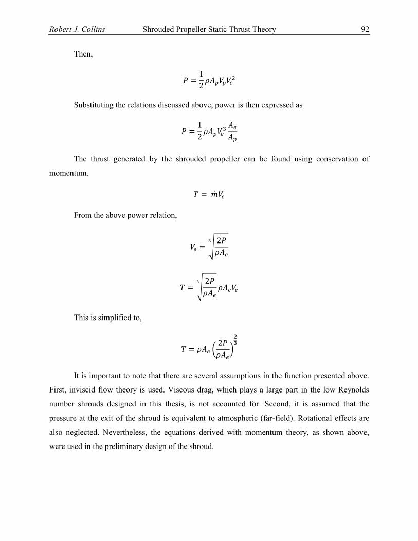
Robert J. Collins Shrouded Propeller Static Thrust Theory 92
Then,
Substituting the relations discussed above, power is then expressed as
The thrust generated by the shrouded propeller can be found using conservation of
momentum.
From the above power relation,
√
√
This is simplified to,
(
)
It is important to note that there are several assumptions in the function presented above.
First, inviscid flow theory is used. Viscous drag, which plays a large part in the low Reynolds
number shrouds designed in this thesis, is not accounted for. Second, it is assumed that the
pressure at the exit of the shroud is equivalent to atmospheric (far-field). Rotational effects are
also neglected. Nevertheless, the equations derived with momentum theory, as shown above,
were used in the preliminary design of the shroud.
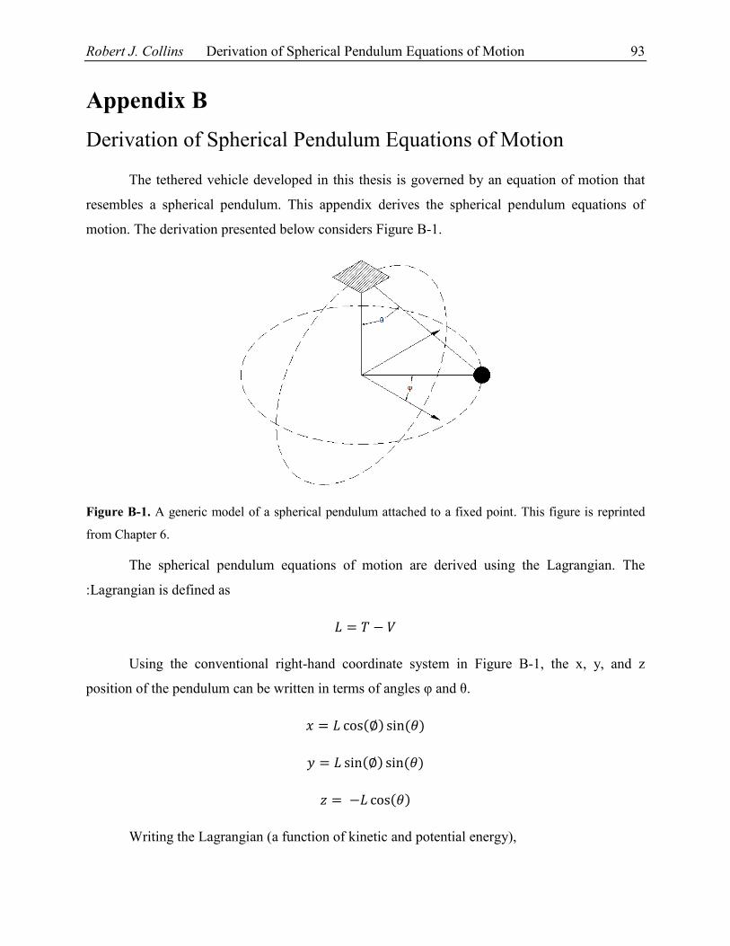
Robert J. Collins Derivation of Spherical Pendulum Equations of Motion 93
Appendix B
Derivation of Spherical Pendulum Equations of Motion
The tethered vehicle developed in this thesis is governed by an equation of motion that
resembles a spherical pendulum. This appendix derives the spherical pendulum equations of
motion. The derivation presented below considers Figure B-1.
Figure B-1. A generic model of a spherical pendulum attached to a fixed point. This figure is reprinted
from Chapter 6.
The spherical pendulum equations of motion are derived using the Lagrangian. The
:Lagrangian is defined as
Using the conventional right-hand coordinate system in Figure B-1, the x, y, and z
position of the pendulum can be written in terms of angles φ and θ.
( ) ( )
( ) ( )
( )
Writing the Lagrangian (a function of kinetic and potential energy),

Robert J. Collins Derivation of Spherical Pendulum Equations of Motion 94
( )
The equations of motion are easily written in terms of the angles φ and θ as opposed to
the rectangular coordinates x, y, and z. Taking the derivative of the x, y, and z relations presented
above, the Lagrangian can be rewritten as,
( ( ) ) ( )
Applying the Euler-Lagrange equations,
(
)
( ) ( ) ( )
This yields the equation of motion,
( ) ( ) ( )

Robert J. Collins Mechanical Prints 95
Appendix C
Mechanical Prints
The following table is a list of mechanical prints for the components of the vehicle that were
machined. Please refer to the page number for the corresponding print.
Component Quantity Page
Shroud Center Body Ring 1 96
Shroud Motor Mount 1 97
Stiffeners 10 98
Floorboard 1 99-106

Robert J. Collins Mechanical Prints 96

Robert J. Collins Mechanical Prints 97

Robert J. Collins Mechanical Prints 98

Robert J. Collins Mechanical Prints 99

Robert J. Collins Mechanical Prints 100

Robert J. Collins Mechanical Prints 101
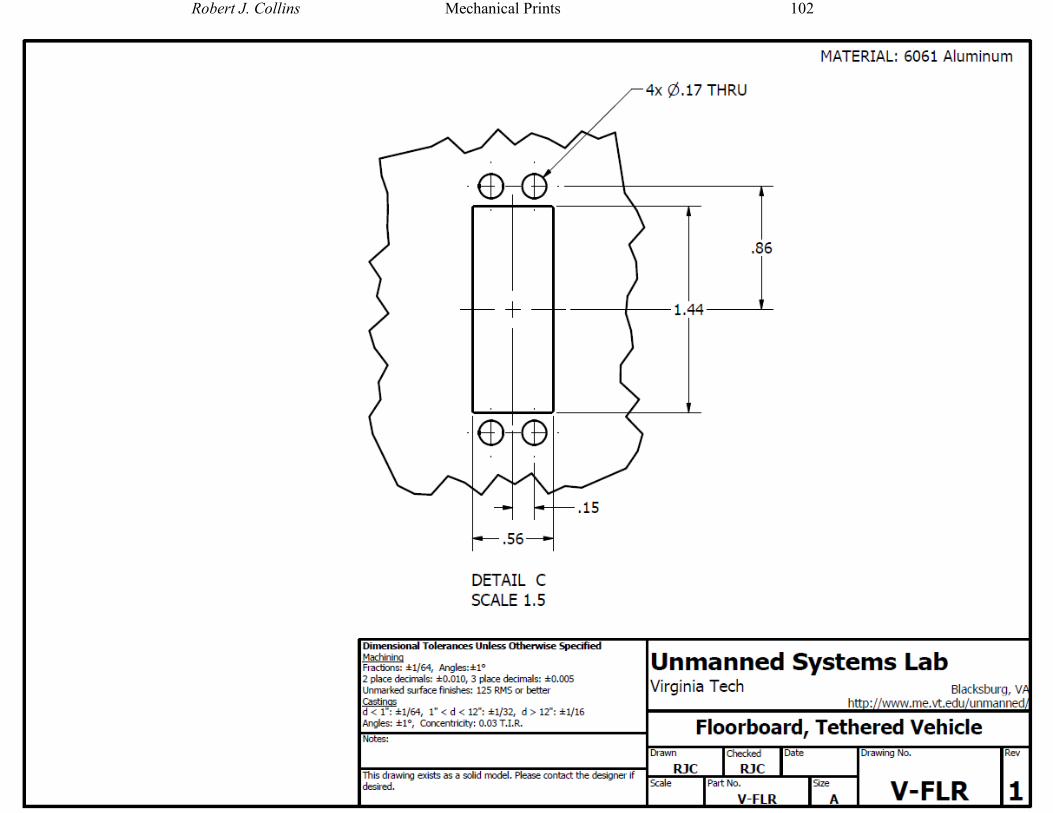
Robert J. Collins Mechanical Prints 102

Robert J. Collins Mechanical Prints 103

Robert J. Collins Mechanical Prints 104

Robert J. Collins Mechanical Prints 105

Robert J. Collins Mechanical Prints 106