Design of a bio-inspired controller for dynamic soaring in ... · Although designing Unmanned...

Design of a bio-inspired controller for dynamic

soaring in a simulated UAV

Renaud Barate, Stephane Doncieux and Jean-Arcady Meyer

Universite Pierre et Marie Curie - Paris 6, UMR 7606, AnimatLab/LIP6, 8 rue du

Capitaine Scott, Paris, 75015 France

E-mail: [email protected], [email protected],

[email protected]

Abstract. This article is inspired by the way birds like albatrosses are able to

exploit wind gradients at the surface of oceans for staying aloft during very long

periods while minimizing their energy expenditure. The corresponding behaviour

has been partially reproduced here via a set of Takagi-Sugeno-Kang (TSK) fuzzy

rules controlling a simulated glider. First, such rules were hand-designed. Then, the

rules were optimized with an evolutionary algorithm that improved their efficiency at

coping with challenging conditions. Finally, the robustness properties of the generated

controller were assessed with a view to its applicability to a real platform.

Keywords : Dynamic soaring, UAV, fuzzy rules, evolutionary algorithm.

This article has been published in Bioinspiration & Biomimetics journal under the

reference:

Renaud Barate, Stephane Doncieux and Jean-Arcady Meyer. “Design of a bio-

inspired controller for dynamic soaring in a simulated unmanned aerial vehicle”.

Bioinspir. Biomim. 1 (2006) 76-88.

Bioinspiration & Biomimetics copyright 2006 IOP Publishing Ltd.

Design of a bio-inspired controller for dynamic soaring in a simulated UAV 2

1. Introduction

Although designing Unmanned Aerial Vehicles (UAV) represents a great challenge for

engineers because such platforms have to face complex and dynamic environments,

numerous research efforts have been devoted to this endeavour and it has now become

relatively easy to build autonomous flying robots, even with off-the-shelf components

[1]. But the decisional autonomy of these platforms is still limited to a capacity to

follow a given trajectory defined by a set of GPS waypoints. For lots of applications,

a higher degree of autonomy is required, that would make it possible to give a robot

watching over forest fires, for instance, a simple order like “stay over this area”. This

would entail providing the robot with a map of its environment and with the capacity

of self-localizing within this map, but would avoid the necessity of pre-defining a series

of waypoints to be followed. More importantly, such an approach would afford the

robot the possibility of autonomously and opportunistically choosing its trajectory, so

as to spare its energy consumption, a major issue for current UAV technology. Indeed,

small-scale fixed-wing UAV – with wingspans less than two meters – currently exhibit

an energy autonomy of one or two hours because they are committed to permanent use

of their motors. If one could find a way to exploit the environment more efficiently, this

autonomy could be widely expanded. To this end, nature is a good source of inspiration

as lots of energy-saving strategies are exploited by birds.

Indeed, some birds are able to fly for very long periods. Albatrosses, for instance,

can spend days in the air without touching the ground. They can reach such a

performance because they are able to remain aloft without flapping their wings, mainly

by exploiting wind gradients, thus saving precious energy. Likewise, birds of prey like

eagles gain altitude by turning inside thermals, and mountain birds like jackdaws exploit

slope-winds to fly without flapping their wings. All these behaviours have been observed

by biologists [2, 3, 4, 5] and exploited by humans to efficiently pilot gliders [6]. However,

in the latter case, the glider is permanently controlled by the human pilot, and the

implementation of energy-saving behaviours in autonomous flying robots has scarcely

been attempted yet, with the notable exception of a recent work [7] on the exploitation

of thermals. The corresponding robot flies until a thermal is found, and then remains

inside it by turning round, thus gaining altitude.

This strategy is only one of those that can be deduced from animal behaviours. It

belongs to the static soaring category because it exploits the air flowing upwards: to

gain altitude, the robot “just” needs to remain inside the thermal. Another strategy,

that belongs to the dynamic soaring category, exploits wind gradients. Here, there is no

upward flow but a horizontal wind, the speed of which varies with altitude, as may be

the case above the ocean or above a mountain slope. To exploit such circumstances and

save energy, a bird or a glider must follow a cyclic trajectory, starting from a relatively

high altitude and flying down, wind in the back. Before hitting the water or the ground,

it must turn back sharply to face the wind, in order to exploit the speed attained during

the dive and so gain altitude. When its relative speed becomes too slow, it must turn


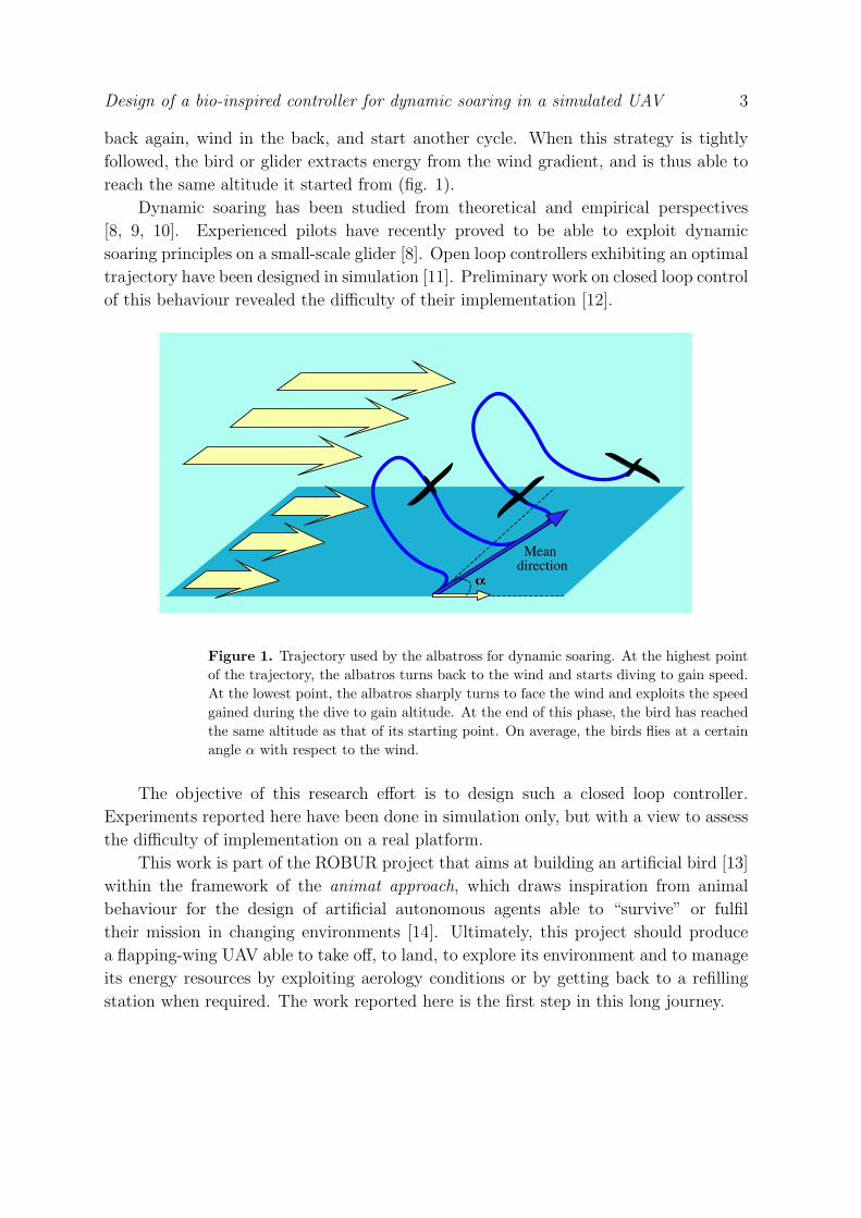
back again, wind in the back, and start another cycle. When this strategy is tightly

followed, the bird or glider extracts energy from the wind gradient, and is thus able to

reach the same altitude it started from (fig. 1).

Dynamic soaring has been studied from theoretical and empirical perspectives

[8, 9, 10]. Experienced pilots have recently proved to be able to exploit dynamic

soaring principles on a small-scale glider [8]. Open loop controllers exhibiting an optimal

trajectory have been designed in simulation [11]. Preliminary work on closed loop control

of this behaviour revealed the difficulty of their implementation [12].

Figure 1. Trajectory used by the albatross for dynamic soaring. At the highest point

of the trajectory, the albatros turns back to the wind and starts diving to gain speed.

At the lowest point, the albatros sharply turns to face the wind and exploits the speed

gained during the dive to gain altitude. At the end of this phase, the bird has reached

the same altitude as that of its starting point. On average, the birds flies at a certain

angle α with respect to the wind.

The objective of this research effort is to design such a closed loop controller.

Experiments reported here have been done in simulation only, but with a view to assess

the difficulty of implementation on a real platform.

This work is part of the ROBUR project that aims at building an artificial bird [13]

within the framework of the animat approach, which draws inspiration from animal

behaviour for the design of artificial autonomous agents able to “survive” or fulfil

their mission in changing environments [14]. Ultimately, this project should produce

a flapping-wing UAV able to take off, to land, to explore its environment and to manage

its energy resources by exploiting aerology conditions or by getting back to a refilling

station when required. The work reported here is the first step in this long journey.


2. Material and Methods

2.1. Flight model

In order to test different controllers designed for dynamic soaring, we developed a

specific flight simulator with a realistic aerodynamic model. This simulator is based

on a perception-action control loop with a time step of 40 ms, which means that 25

times per second the controller provides orders to the glider’s actuators, according to

the current state of its sensors. Wings are made of two panels with different dihedral

angles – i.e. 2o for the internal panel and 6o for the external – to improve the stability

of the glider.

Figure 2. The different controls of the simulated glider : ailerons, elevators, and

rudder.

The aerodynamic model integrates the forces exerted on the two panels that

constitute a wing, and on the two perpendicular surfaces that characterize the tail

(fig. 2). These forces depend on the characteristic curves that describe how the lift (Cz)

and drag (Cx) coefficients vary with a panel’s angle of attack [15]. The aerodynamic

force exerted on each panel is calculated according to the following formula [16]:


~FA =

−CX

0

−CZ

ρSVA2

2

~FA being the aerodynamic force exerted on a given panel, ρ the air density, S the

area of the panel, and VA the airspeed.

Aerodynamic forces on the body part of the glider are neglected here. The

independent calculations of the forces on each panel allow the model to take implicitly

into account some aerodynamic effects such as induced drag, environmental vortices, and

wind gradients. Indeed, in a wind gradient, the airspeed of each panel will be different,

and the resulting aerodynamic forces and momentums will reflect these differences. The

characteristic curves of the panels are calculated to take into account the panel’s aspect

ratio. Figure 3 shows the resulting lift/drag ratio when the independant forces are

integrated to calculate the aerodynamic force applied on the whole glider. However, it

should be noted that the turbulences and vortices generated by the glider’s geometry

are not taken explicitly into account. Aerodynamic ground effect is also not modelled

here. Although this choice can be discussed, we consider that the short period spent

near the ground, and the high bank angle at this point of the trajectory, allow us to

safely ignore this effect.

-20

-10

0

10

20

30

-20 -15 -10 -5 0 5 10 15 20 25

CZ

/ C

X

Angle of attack (degrees)

2m wing span (aspect ratio 8)2.75m wing span (aspect ratio 15.125)

3.5m wing span (aspect ratio 24.5)

Figure 3. Variation of the lift/drag factor (CZ/CX) according to the angle of attack

for the whole glider. Aspect ratios are taken into account in the calculation of the

characteristic curves of each panel. The total wing area is held constant at 0.5 m2, no

sideslip effect is present here.


These aerodynamic forces are then integrated using classical solid body equations

to determine the global linear and angular accelerations of the glider. Its weight is

added to these forces and the system’s state (position and velocity) is updated at each

time-step.

In this simplified aerodynamic model, the controls of the glider are assumed to

modify the angle of attack of its panels. Each swivelling control surface is thus

characterized by an efficiency coefficient ksi with i = 0 for the ailerons, i = 1 for

the elevator, and i = 2 for the rudder. This coefficient is roughly equivalent to the

proportion of the panel’s surface it occupies. We chose:

• ks0 = −0.12 (it has the same value for the internal and the external parts of a wing)

• ks1 = −0.15

• ks2 = −0.5

The amplitude of the controller’s action on a particular control surface is

represented by a value di (d0 = A corresponds to the aileron command, d1 = E is

the elevator command and d2 = R is the rudder command, as explained later on)

comprised between -1 and +1, which is assumed to modify the angle of attack αRi of

the corresponding panel according to the formula: αMi = αRi + di ∗ ksi, where αMi is

the modified value.

Hopefully, this procedure provides a realistic enough simulation to make it possible

to re-use the controllers thus generated on a real motorized glider. Be that as it may,

although this simulation is based on a motorized glider geometry, the corresponding

propulsion capacities are never used, and only the wind serves to move the UAV. Its

physical characteristics are accordingly set to:

• Mass: 3.6 kg

• Length: 1.5 m

• Wing span: 2.75 m (variable in the experiment described in subsection 3.2)

• Total wing area: 0.5 m2 (70% for the internal panel, 30% for the external panel)

• Wings sweep angle: 0o

• Wings dihedral angle: 2o for the internal panel and 6o for the external panel

• Wings twist angle: 2.5o

More details about the mass characteristics of the glider are presented in Appendix

A.

2.2. Wind model

The vertical wind gradient that may be used for dynamic soaring above the ocean

stretches over a thin layer (a few meters) in which the wind is slowed down by the

interactions with the water surface. Observations made for winds of low to medium

speed indicate that this gradient may be represented as a logarithmic function [17].


More precisely, we used the function described in [9] which defines the wind-speed VWat altitude h as:

VW = VWREF

log(h/H0)

log(HREF/H0)

HREF is the reference altitude, i.e., 10 meters in this application.

H0 is the altitude at which the wind-speed equals zero, here it is set to 0.03 meters.

VWREFis the wind-speed at reference altitude. Its default value is 20 m/s. This

speed will occasionally be changed in some experiments described later.

The wind gradient described by this function is presented on Fig. 4.

0

2

4

6

8

10

12

14

16

0 5 10 15 20 25

Alt

itu

de

(m)

Wind speed (m/s)

Wind gradientReference wind speed

Figure 4. Wind-speed gradient used in the model

2.3. Sensors and controls

The sensory system of birds has not been thoroughly studied yet, but some relevant

observations have been made [18]. Briefly, birds possess the same kind of visual receptors

as humans (rods and cones) but they can discriminate colours better, see ultra-violet

light, and perceive light polarization. They also have magnetic receptors, acting like

compasses. Their tactile perception allows them to precisely sense pressure, pressure

change, and pressure change acceleration, thus affording important information about

air speed and air acceleration.

Nevertheless, because a long-term objective of this work is to apply it to a real

glider, sensors as complex as those of birds weren’t used here. Instead, we relied on


more classical sensors to get the data necessary for flight control: an altimeter to get

the glider’s altitude, and an inertial measurement unit to get orientation angles. The

variables measured by these sensors were:

• z, glider’s altitude,

• ψ, glider’s heading with respect to the wind

• θ, glider’s pitch angle with respect to an horizontal plane

• ϕ, glider’s bank angle with respect to an horizontal plane.

We first considered that these sensors were perfect, in the sense that they were

expected to provide exact values in real time. Later on in this paper, the influence of

noisy sensors on the generated behaviour will be studied.

To control the glider, classical effectors were used, i.e., a pair of ailerons, a pair of

elevators, and a rudder (fig. 2). As explained above, the corresponding variables were:

• A, aileron command comprised between -1 (maximum bank to the right) and +1

(maximum bank to the left);

• E, elevator command comprised between -1 (maximum upward) and +1 (maximum

downward);

• R, rudder command comprised between -1 (maximum on the right) and +1

(maximum on the left).

2.4. TSK fuzzy rules

Controllers based on fuzzy rules have been successfully used for the control of several

UAV systems [19, 20]. Their main advantage is to call upon explicit rules, unlike neural

networks whose inner workings may be difficult to decipher. They are particularly well

suited for dealing with incomplete or uncertain data. The corresponding rules can be

hand-designed by a human, or automatically generated by an evolutionary algorithm.

The principle of such fuzzy controllers consists in designing a set of rules that

associate a particular action to a given sensory state. Such rules are made up with a

condition part and an action part. The former may refer to fuzzy sets associated with

each input, e.g., “IF z is low AND z is greatly negative”. The sum of the membership

values of each input variable gives the strength of the rule. The latter may be fuzzy

or not. Rules with fuzzy actions are called Mamdani rules [21], and sometimes require

a tricky defuzzification procedure to generate the orders to be send to the system’s

actuators. Instead, in this work, we used Takagi-Sugeno-Kang (TSK) rules [22] for

which the consequent of a rule is not a fuzzy set but a linear combination of the input

variables. This method allows faster calculations than classical defuzzyfication methods.

Thus, a typical TSK fuzzy rule would be for example “IF z is low AND z is greatly

negative THEN E = 0.25 + 0.5z − 0.25z”.

It is also simple to make TSK fuzzy rules evolve via an evolutionary algorithm, as

demonstrated, for instance, with the control of a real helicopter [23]. Fuzzy sets limits


and rule coefficients being simple real numbers, it’s easy to define the corresponding

cross-over and mutation operators, a point that will be touched on later in this section.

2.5. The controller’s bio-inspired design

In a first stage, we hand-designed a reference controller with rules inspired by

observations of real albatrosses. This way, we checked that a TSK controller is well

suited for this problem and we set a base for further evolutionary improvements.

In his 1982 observations [2], Pennycuick described the dynamic soaring behaviour

in these terms:

A bird soaring across wind, along a wave, would from time to time turn into

wind and pull up sharply, then turn at the top of the climb and glide off again

across wind. The turns initiating and completing this manoeuvre were often

abrupt and very steeply banked, up to 70o. This behaviour was seen in all the

albatross species, and also in the giant petrel and white-chinned petrel.

Consequently, we decided to decompose the dynamic soaring behaviour of our

controller into two phases:

• an ascending phase in which the bird faces the wind and gains altitude,

• a descending phase in which the bird is back to the wind and dives to gain speed.

More precisely, we wrote two sets of rules: one for turning toward the wind origin

when the glider is low (ascending phase), and one for turning back to the wind when

it is high (descending phase). The corresponding fuzzy sets were defined by ramp-type

membership functions (Fig. 5).

The turns defined by these two sets of rules need to be very sharp, therefore they

were triggered using the elevators with a very high bank angle. The rudder was used to

prevent the glider from plunging right down to the sea. As for the ailerons, they were

used to maintain the bank angle. With these principles, we wrote the first rules for the

reference controller. Then we empirically improved the values defining the fuzzy sets,

as well as other parameters of the rules, until we obtained an improved and coherent

behaviour. Here are the details of the three hand-designed rules for turning back to the

wind:

• When the glider is high, the elevators must be raised in order to trigger a sharp

descent, but they also have to control the pitch angle to prevent the glider from

diving too quickly. They also must get lowered at the end of the turn, when

the glider is almost back to the wind. Therefore, the first rule is ”If z is high,

E = −0.6 + 0.01θ + 0.006(ψ + 180)”.

• When the glider is high, it turns sharply to the right‡. The rudder must then be

put to the left in order to prevent the glider from diving due to the high bank

‡ We arbitrarily chose this direction, with the consequence that the glider moved from north-west to

south-east.


0

0.2

0.4

0.6

0.8

1

0 2 4 6 8 10 12 14 16

Deg

ree

of

mem

ber

ship

Altitude (m)

z is lowz is high

Figure 5. Fuzzy sets defined on variable z (altitude). Two sets are defined,

respectively for high and low altitudes, the corresponding degree of membership

progressively changing according to the glider’s altitude. In other words, when the

latter is lesser than five meters, the system’s altitude has more chances to be classified

as “low” than as “high”.

angle§. The corresponding R value depends on the bank angle itself, and on the

heading in order to trigger diving when the turn ends. Therefore, the second rule

is ”If z is high, R = −1.0 + 0.006(ψ + 180) + 0.01ϕ”.

• When the glider is high, we use the ailerons to increase the bank angle for the

turn to the right. The value for the ailerons depends on the bank angle because

we want to stabilize it, and on the heading because we want to decrease the

bank angle at the end of the turn. Therefore, the third rule is ”If z is high,

A = −1.0 + 0.006(ψ + 180) + 0.007ϕ”.

The three rules for turning toward the wind rely on the same principles:

• If z is low, E = −0.8 + 0.02θ + 0.005(ψ + 180) ;

• If z is low, R = 0.006(ψ + 180) + 0.01ϕ ;

• If z is low, A = 0.006(ψ + 180) + 0.007ϕ.

The positions of the control surfaces in each phase of the trajectory are shown

in figure 6. Here we assume that the wind blows from north to south. It should be

mentioned that the rules just described allow dynamic soaring in one direction only,

§ In this configuration, the rudder is almost horizontal and acts like the elevators in the glider’s nominal

position


i.e., from the north-west to the south-east. To prompt flights from north-east to south-

west, we just have to replace ψ by (360 − ψ), ϕ by −ϕ and to change the sign of the

rules for R and A. We will describe in section 3.3 some experiments we made to evolve

controllers able to fly in different directions.

In fact, it appeared that this hand-designed reference controller exhibited the kind

of behaviour we were interested in, but it was not really efficient. More specifically, it

worked only when the wind-speed was high enough, and it failed to keep the glider aloft

beyond four complete cycles. Nevertheless it constituted a good starting point for its

improvement via an evolutionary algorithm, as described in the following section.

2.6. Evolutionary optimization

The goal of the evolutionary algorithm described here was to generate a more efficient

and more robust soaring behaviour. This algorithm was initialized with the hand-

designed rules of the reference controller just described.

The genome of each controller was represented by a vector of real variables, each

number corresponding to a rule parameter, or to a boundary of the altitude fuzzy

set. Each generation of controllers but the first contained 100 individuals, and the

experiments involved 100 generations. The first generation contained 1000 individuals

in order to increase the number of interesting controllers at the beginning of the

evolutionary run, and thus to accelerate the convergence of the algorithm.

In each generation, the 20 best individuals were kept, while the other 80 individuals

were deleted (980 in the first generation) and replaced by 80 new ones. The fitness

criteria that were used depended on the experiments that were performed, and will be

described in the next section. Each creation of a new individual was done in two steps:

first a cross-over, then a mutation.

For the cross-over, two individuals were randomly selected from among the survivors

of the previous generation. The probability of selection depended on individual rankings,

individuals with higher fitnesses being chosen more often than those with lower fitnesses.

Each gene of a new individual was then inherited from one of its parents with an equal

probability.

Mutations consisted of slightly changing the value of each gene. The mutation of a

gene value γ was defined by:

γt+1 = γt + N (0, µ ∗ τ)

where the function N (0, µ ∗ τ) represents a normal distribution of zero mean and

standard deviation µ ∗ τ . µ is a mutation factor defined for each gene, and τ is

an attenuation factor τ which decreases the amplitude of the mutations in the last

generations. Methods for automatically adapting the mutation rate exist [24, 25], but

the use of an attenuation factor, as done here, lead to quicker convergence than such

alternative procedures.

The mutation factor µ was defined by:


Figure 6. Glider’s trajectory and position of its control surfaces in each phase. See

text for details.


• µ = 0.1 for genes corresponding to rule parameters,

• µ = 1.0 for genes corresponding to altitude fuzzy set boundaries.

The attenuation factor τ has been determined empirically. For generation g it was

defined by equation:

τ = exp(

−g

20

)

3. Experiments and results

3.1. Low wind-speed conditions

The first series of experiments consisted in using the evolutionary algorithm just

described to generate controllers able to secure a dynamic soaring behaviour in lower

wind-speed conditions than those required by the reference controller. To limit

simulation time, we assessed the fitness of an individual by the minimal wind-speed

that maintained it aloft for 1000 seconds, and tried to minimize this value.

For each individual, this process started with the nominal wind-speed to which the

reference controller was adapted – i.e., 20 m/s – and proceeded with a dichotomous

search. Individuals that could not fly for the whole of the evaluation period, even with

the reference wind speed, were ranked according to how long they stayed aloft.

For each generation, if the necessary wind-speed for the twentieth and less adapted

individual was less than the current reference wind speed, the corresponding value

became the new reference speed to be used for next generations. This procedure greatly

accelerated the computations.

Figure 7 shows the results obtained along 100 generations. It appears that the

best individual thus generated is able to exhibit a dynamic soaring behaviour with a

wind-speed of only 9.4 m/s. By comparison, the minimum wind-speed needed by the

albatross seems to be about 8.6 m/s [9].

It is interesting to compare the trajectory used by the reference controller with the

one used by the best evolved controller (Fig. 8 and 9). The first loses altitude in each

cycle and ends up in the water after only four cycles. The second keeps a constant

altitude at the top of each cycle and rapidly follows a periodical trajectory, although

the wind-speed is twice lower.

Table 1 summarizes the differences between the hand-designed controller and the

evolved one. These differences are neither negligible nor reflecting drastic changes. They

suggest that the design of dynamic soaring controllers, like those considered here at least,

is a difficult task, as small changes in the corresponding parameters may cause a glider

to operate perfectly well, or to crash after a few cycles only. This remark probably

explains why we never succeeded to evolve such controllers from scratch, and why they

proved to be sensitive to turbulences and sensory noise, as mentioned in section 3.4

below.


8

10

12

14

16

18

20

0 10 20 30 40 50 60 70 80 90 100

Min

imu

m w

ind

sp

eed

(m

/s)

Generation

Best individualReference speed

Figure 7. Evolution of the minimal wind-speed that secures dynamic soaring in the

simulated glider

0

5

10

15

20

25

0 100 200 300 400 500 600 700

Alt

itude

(m)

X (m)

Trajectory (longitudinal)End point

0

5

10

15

20

25

-20 -15 -10 -5 0 5 10

Alt

itude

(m)

Y (m)

Trajectory (transversal)End point

Figure 8. Longitudinal and transversal projections of the glider’s trajectory with the

reference controller (wind-speed : 20 m/s). The flight is not regular and ends after

four cycles at the “End point”.

3.2. Wing aspect ratio

The goal of this series of experiments was to evaluate the morphology of a real glider on

which the dynamic soaring behaviour studied here could be implemented. To this end,

we compared results obtained by changing the glider’s wing aspect ratio ARW , defined

as the ratio of the wing span SW and the chord CW for a rectangular wing, or as the

ratio of the squared wing span and the wing area AW for a wing of any shape (fig. 10):


0

5

10

15

20

25

0 200 400 600 800 1000 1200 1400

Alt

itude

(m)

X (m)

Trajectory (longitudinal)

0

5

10

15

20

25

-50 -40 -30 -20 -10 0 10 20

Alt

itude

(m)

Y (m)

Trajectory (transversal)

Figure 9. Longitudinal and transversal projections of the glider’s trajectory with the

best evolved controller (wind-speed : 10 m/s). The flight quickly becomes cyclic and

the altitude at the top of each cycle remains constant.

Hand-designed controller Evolved controller

Fuzzy sets

z is high, Ramp bounds 5.0 → 13.0 3.095691 → 11.452055z is low, Ramp bounds 2.0 → 9.0 1.857289 → 8.453340

Rules

z is high, E = −0.6 + 0.006(ψ + 180) + 0.01θ −0.599127 + 0.004392(ψ + 180) + 0.006740θz is high, G = −1.0 + 0.006(ψ + 180) + 0.01ϕ −1.056806 + 0.002087(ψ + 180) + 0.008521ϕz is high, A = −1.0 + 0.006(ψ + 180) + 0.007ϕ −0.831355 + 0.003803(ψ + 180) + 0.014658ϕz is low, E = −0.8 + 0.005(ψ + 180) + 0.02θ −1.288160 + 0.006382(ψ + 180) + 0.020173θz is low, G = 0.0 + 0.006(ψ + 180) + 0.01ϕ 0.000793 + 0.011099(ψ + 180) + 0.006601ϕz is low, A = 0.0 + 0.006(ψ + 180) + 0.007ϕ −0.002391 + 0.009162(ψ + 180) + 0.012029ϕ

Table 1. Comparison between hand-designed and automatically-evolved rules.

ARW =SWCW

=SW ∗ SWCW ∗ SW

=S2W

AW

In these experiments, we increased the wing aspect ratio by increasing the wing

span and decreasing the wing chord. The wing area and mass were held constant all

the while. Again, an evolutionary approach was used to seek the lowest wind-speed

compatible with dynamic soaring for a variety of aspect ratios. The corresponding

results are shown in figure 11.

These results show that dynamic soaring can be efficiently performed for aspect

ratios varying between 12 and 21. As a comparison, the aspect ratio of an albatross’

wing roughly equals 18 [9]. The existence of a lower limit can be related to the fact

that a low aspect ratio decreases the lift, and increases the drag of the wing. This

explains why gliders and migratory birds have wings with high aspect ratios. As for

the existence of an upper limit, it has to do with the nature of the trajectory used for

dynamic soaring. Indeed, when the glider is near the water, it makes a sharp turn on

the wing to face the wind. The bank angle is then very high, which means that a glider

with a 2-meter wing span won’t be able to get much lower than 1 meter before hitting

the water. The wind gradient being more important in the first meters above water,


Wing span

Wing area

Wing chord

Figure 10. Characterization of the wing span, the wing chord, and the wing area

that serve to calculate the wing’s aspect ratio.

8

9

10

11

12

13

14

8 10 12 14 16 18 20 22 24 26

Win

d s

pee

d

Wing aspect ratio

Minimum necessary speed (best results)Mean results and standard deviations

Albatross values

Figure 11. Minimum necessary wind-speed as a function of wing aspect ratio.

Efficient dynamic soaring, i.e., under slow wind-speed conditions, can be performed

for wing aspect ratios varying between 12 and 21.


a high aspect ratio can prevent efficient dynamic soaring, as it will prevent the glider

from going low enough to take advantage from the steepest part of the gradient‖.

3.3. Soaring direction

In the experiments just described, the goal for the glider was merely to stay aloft for the

longest time, and the average direction of the glider was not taken into account in the

fitness. In fact, the reference controller generates a trajectory whose overall direction

is oriented from north-west to south-east with a wind blowing from the north. Here,

we wanted to assess the possibility of evolving controllers able to move the glider in

different directions, against the wind for instance.

To this end, we changed the fitness function in order to select individuals that flew

in a given direction. More precisely, the corresponding fitness function was the difference

between the glider’s mean heading and the target’s heading, the goal being to minimize

this function. The heading variable ψ being defined as the angle between the wind and

the glider’s heading, the fitness function f(ind) was set to f(ind) = abs(ψmean−ψtarget).

For each generation, we selected the individuals whose headings were the closest to the

target’s one.

Only two experiments were made in order to determine the full range of directions

that could be achieved with the kind of controllers studied here. The first one sought

controllers generating flights against-the-wind (target heading = 180o), while the second

one sought controllers generating back-to-the-wind flights (target heading = 0o). These

experiments made it possible to determine the minimum and maximum angles relative

to the wind that delimit the directions in which the glider can fly.

Results obtained during the first experiment indicate that the maximum angle

between the glider’s heading and the wind’s origin was 53o. In the second experiment,

the minimum angle was 8o.

Inasmuch as symmetrical flying-angle values may be attained by making

appropriate changes in a controller’s fuzzy rules, it appears that angles between 8 and

-8o can be reached by adequately switching the desired direction between these two

values¶. It may be concluded from this section that the full range of flying directions

afforded by the variety of controller investigated in this work is [−53o; 53o] (Fig. 12).

To appreciate the significance of these results, we thoroughly examined the flying

behaviours generated by three evolved controllers: the one corresponding to a mean

heading of 53o – the maximum value –, the one corresponding to a mean heading of

8o – the minimum value –, and one corresponding to a mean value of 30o – arbitrarily

chosen in the preceding interval. The details of the rules that correspond to these three

controllers are given in Appendix B.

‖ As our evolved controller brings the glider down to 1.32m, one of its wings is approximately 0.15m

above the water during the sharp turn (wing length of 1.375 and bank angle of 58o).¶ if the glider spends 50% of its trajectory oriented toward 8o and 50% oriented toward -8o, the glider

direction will be 0o on average.


Figure 12. The range of average directions toward which a glider can fly using the

controllers evolved in this work.

It thus appears that these controllers implement different strategies. In particular,

the 53o controller oscillates less than the others (Fig. 13b, 13c, 13d) and remains

approximately between 0 and 10 meters whereas other controllers reach far higher

altitudes (Fig. 13a). The movement direction imposed by the 53o controller is almost

always further from the wind than those corresponding to the other controllers, even

reaching a peak at 90.5o (Fig. 13e). The movement direction angle is greater in the lower

part of the cycle than in the higher part for all three controllers. This is particulary

true with the 53o controller that makes the glider fly lower than with the two other

controllers : this way, it avoids being carried by the wind which is stronger at higher

altitudes.

With respect to the two other controllers, it also appears that the “53o” one

generates greater forces serving to accelerate along the lateral axis during the period

when the altitude is high (table 2). Such strategy increases the lateral speed of the

glider during the first cycles, with the consequence that it also increases the drag during

this critical phase that makes it possible to gain kinetic energy (Fig. 14 and 15). As a

result, the farther the glider is relatively to the wind direction, the more energy it looses.

According to our results, 53o seems to be the greatest angle for which an equilibrium

can be found, at least in the experimental setup used here.

These results stress the limits of our approach focussed on dynamic soaring only.


0

10

20

30

40

50

42 44 46 48 50 52 54

Alt

itude

(m)

Time (s)

8o

30o

53o

-150

-100

-50

0

50

100

42 44 46 48 50 52 54

Hea

din

g ψ

(o)

Time (s)

8o

30o

53o

(a) (b)

-60

-40

-20

0

20

40

60

80

100

42 44 46 48 50 52 54

Pit

ch θ

(o)

Time (s)

8o

30o

53o

-100

-50

0

50

100

150

42 44 46 48 50 52 54

Roll

φ (

o)

Time (s)

8o

30o

53o

(c) (d)

0

50

100

150

42 44 46 48 50 52 54

Movem

ent

dir

ecti

on (

o)

Time (s)

8o

30o

53o

(e)

Figure 13. Altitude (a), orientation angles (heading (b), pitch (c) and roll (d)) and

movement direction (e) of a glider flying toward three different mean directions : 8o,

30o and 53o relative to the wind. Data for 8o and 30o have been respectively shifted

by 2.4 s and 1.5 s, to synchronize the beginning of each cycle.


-10

-5

0

5

10

15

20

25

30

35

40

13 14 15 16 17 18 19 20

Forc

e (N

), A

ltit

ude

(m)

Time (s)

Fx 53Fx 30 (shifted)Fx 8 (shifted)

Altitude 53 (m)Average altitude 53

Figure 14. Resultants of aerodynamic forces projected on the longitudinal axis of the

glider (Fx). Fx is lesser with the 53o controller than with the two others. In particular,

it is negative and, most of the time, smaller than the others when z is greater than

zavg.

0

500

1000

1500

2000

2500

3000

13 14 15 16 17 18 19 20

Ener

gy (

J), A

ltit

ude

(1/1

00 m

)

Time (s)

kinetic energy 53kinetic energy 8 (shifted)

kinetic energy 30 (shifted)Altitude 53

Average altitude 53

Figure 15. Kinetic energy variations for controllers generating flights in different

directions. 6.9m being the average value of altitude corresponding to the 53o-controlled

glider, the period when altitude exceeds this value corresponds to the acceleration phase

of the glider. This acceleration is lesser for the 53o controller than for the other two.

Kinetic energies corresponding to the 30o and 8o controllers are shifted in time by resp.

1.1s and 1.8s, in order to synchronize the three cycles.


53o 30o 8o

Average Fyabs (N) 0.69 0.34 -0.08

Average altitude zavg (m) 6.9 15.5 19.6

Average Fyabs(N)

for z > zavg 14.9 3.98 -3.79

for z < zavg -12.19 -3.6 2.9

Table 2. Average value of projection on the Y-axis of the sum of aerodynamic forces

in the absolute frame. These values correspond to the first 60s of a test flight and

accordingly mostly characterize the transient phase. At steady state, the average

value of Fyabs is null, as the lateral speed is constant.

Indeed, the glider is unable to follow a trajectory that is, on average, directed against

the wind, a performance of which albatrosses are perfectly capable. This is due to the

fact that these birds may use other means than dynamic soaring for flying without

self-propulsion. For instance, Pennycuick observed albatrosses flying without flapping

their wings with a very low wind, or even with no wind at all [2] and, because dynamic

soaring is impossible in these conditions, he suggested that another source of energy is

used by these birds:

The observations suggest [...] that in practice most of the energy for windward

pullups comes from slope lift [...] and relatively little from the wind gradient.

The wind gradient may supply relatively more energy in downwind flight, but

no direct observations were obtained to support this.

It would therefore be necessary to model such slope currents along the waves to be

able to reproduce the trajectories of albatrosses more precisely.

3.4. Control robustness

Other experiments were run to test the robustness of the controllers developed here.

More precisely, we evaluated their robustness to variations in initial conditions, to wind

turbulences, and to sensory noise. It should be noted that these experiments were not

designed to assess a controller’s robustness to particular conditions, which would require

a much more realistic environmental model, but rather to evaluate the genericity of the

evolved controllers. We only look for an answer to the question “Are these controllers

able to cope with slight changes in the environment ?”. Answers to the questions “Are

these controllers able to cope with a real environment ?” and “Are these controllers

able to adjust their behaviour depending on the environment ?” are, of course, related

to this study, but they will be investigated thoroughly in a future work.

Concerning robustness to initial conditions, we evolved controllers as we did in the

first experiment, but starting with a wider range of altitude, heading and relative speed

conditions. These conditions were set at random in the following ranges:


−135o − δ ∗ 10o < ψ < −135o + δ ∗ 10o

15 m − δ ∗ 0.5 m < h < 15 m + δ ∗ 0.5 m

20 m/s − δ ∗ 0.5 m/s < V < 20 m/s + δ ∗ 0.5 m/s

If ten consecutive runs were successful – i.e. if the glider could remain aloft for the

whole experiment – we considered the individual as adapted to the variation rate δ.

The results that were obtained indicate that the best evolved controllers were able

to stand a variation rate of 9, which means they could maintain dynamic soaring with

initial conditions in the ranges:

−225o < ψ < −45o

10, 5 m < h < 19, 5 m

15, 5 m/s < V < 24, 5 m/s

Concerning robustness to turbulences, the fitness function was the maximum

amplitude of wind-speed perturbations tolerable to the controller. These perturbations

were represented as a noise vector added to the reference wind vector. At each time

step, the noise vector amplitude was modified by a random value between -0.04 and

+0.04 m/s and its heading was modified by a random value between -0.6 and +0.6o

(corresponding to a maximum change rate of 1 m/s/s and 15o/s). This noise vector

is added to the reference wind vector. Winds at other altitudes are then computed as

stated in section 2.2, so the noise is less important at lower altitudes where the wind is

slower.

Controllers able to keep the glider aloft for ten consecutive experiments with a given

maximum turbulence amplitude were considered adapted to this noise level. Results

indicate that the best evolved controllers were able to stand a maximum turbulence

amplitude of 1.7 m/s for a reference wind set at 20 m/s.

Finally, to assess the robustness to sensory noise, we did not use evolution. Instead,

we simply tested the controller evolved in the experiment described in subsection 3.1,

using a reference wind speed of 10 m/s and adding to the sensors a gaussian noise

with a zero mean and a standard deviation that was systematically varied. The results

presented here correspond to the maximum standard deviation value for which ten

consecutive experiments were successful, in the sense that the glider remained aloft for

more than 1000 seconds:

• Maximum standard deviation for noise on altimeter: 0.09 m

• Maximum standard deviation for noise on ψ: 1o

• Maximum standard deviation for noise on θ: 1o

• Maximum standard deviation for noise on φ: 1.5o

Although such results seem to indicate that robust control requires a sensory

precision that exceeds that of current off-the-shelf devices, it is still possible that

this conclusion will have to be amended if more robust controllers are sought through


improved evolutionary approaches. For instance, one could select individual able to

simultaneously cope with a low and turbulent wind, on the one hand, and with noisy

sensors, on the other hand. Likewise, it is still possible that more robust controllers will

be generated using rules better adapted to sensory noise and environmental conditions

than those that were used here.

4. Discussion

The main advantage of the dynamic soaring controllers described in this article is the

simplicity of their design and optimization : a first controller has been hand-designed and

then optimized by evolutionary algorithms. The trajectories these controllers generate

are very similar to those exhibited by albatrosses above the ocean, thus demonstrating

that such a natural behaviour can be implemented with few simple fuzzy-rules.

However, if they are able to keep a glider aloft in low wind conditions similar to

those an albatross can cope with during dynamic soaring, these controllers can’t get

energy from other aerological conditions, like slope wind, which this bird is able to

exploit for flying without flapping its wings. These conditions allow it to fly against the

wind for example, a behaviour that the controllers studied here are unable to exhibit.

To reach a performance similar to that of an albatross, several other controllers should

be designed, for instance a series of low-level controllers able to exploit other aerological

conditions, and a high-level controller able to switch between different behaviours, i.e.

from static soaring to dynamic soaring.

Despite the fact that the apparent lack of robustness of the controllers studied here

to noisy sensors, or to wind turbulence, could probably be improved with appropriate

evolutionary approaches, controlling dynamic soaring is intrinsically a difficult problem

because the corresponding trajectories must be very precise. In particular, when a glider

flies at a few centimetres above the ocean’s surface, small errors in sensors, or small wind

turbulences, may be enough to make it touch the water. To help avoid such a fatal issue,

robust filtering methods could be used, as well as avoidance-strategies based on optical

flow that have already proved to be efficient in similar contexts [26]. Likewise, other

rules could be tried that would hopefully correct the trajectory more often and more

precisely.

It is also interesting to note that, if the wing aspect ratio is kept small enough,

the parameters of the controllers obtained after evolution show only small differences

compared to those of the reference controller. This however has a great impact on

the performance of the glider, thus suggesting that the generated trajectories are very

sensitive to these parameters. This renders the evolution of such a controller from

scratch extremely difficult, as this process will get a substantial reward only when it is

near the optimal solution. Indeed, very few solutions have a high fitness, the majority

of them, especially those of the first generations, being characterized by low fitness

values that cannot guide evolution. It is highly probable that, even with other sorts

of controllers – e.g., neural networks – or with a different set of fuzzy rules, the same


bootstrapping difficulty would be experienced because of the required precision in the

generated trajectories.

5. Conclusion

Although dynamic soaring is a complex behaviour that needs to be very precisely

controlled, the results that have been presented here demonstrate that it may be

generated by a set of simple fuzzy rules bootstrapped by an educated guess. These

results also suggest that the implementation of such rules on a real glider capitalizing

on simple off-the-shelf sensors is possible, provided the corresponding platform is not

used in too challenging conditions, i.e., with a too low and turbulent wind, or with too

noisy sensors, and provided trajectories against the wind are not sought. Some hints

for relaxing these constraints have been given in the text.

6. Acknowledgements

This work was supported by a BQR grant from Pierre and Marie Curie University

(Paris 6). The authors wish to thank Thierry Druot for the development of the flight

simulator and for his help with the analysis of the huge amount of data produced by the

simulation. They also express their gratitude to the reviewers for their help in improving

the manuscript.

References

[1] http://www.nongnu.org/paparazzi/.

[2] C. J. Pennycuick. The flight of petrels and albatrosses (Procellariiformes), observed in South

Georgia and its vicinity. Phil. Trans. R. Soc. Lond. B, 300:75–106, 1982.

[3] R. Spaar and B. Bruderer. Migration by flapping or soaring: flight strategies of Marsh, Montagu’s

and Pallid Harriers in southern Israel. The Condor, 99(2):458–469, March-April 1997.

[4] N. G. Smith, D. L. Goldstein, and G. A. Bartholomew. Is long-distance migration possible for

soaring hawks using only stored fat? Auk, 103(3):607–611, July-September 1986.

[5] A. Hedenstrom, M. Rosen, S. Akesson, and F. Spina. Flight performance during hunting excursions

in Eleonora’s falcon falco eleonorae. The Journal of Experimental Biology, 202:2029–2039, 1999.

[6] J. Parle. Preliminary dynamic soaring research using a radio control glider. In 42nd AIAA

Sciences Meeting and Exhibit, Reno, Nevada, 5-8 january 2004. AIAA Paper 2004-132.

[7] M. J. Allen. Autonomous soaring for improved endurance of a small uninhabited air vehicle. In

43nd AIAA Sciences Meeting and Exhibit, Reno, Nevada, 10-13 january 2005. AIAA Paper

2005-1025.

[8] M. B. E. Boslough. Autonomous dynamic soaring platform for distributed mobile sensor arrays.

Technical report, Sandia National Laboratories, 2002.

[9] G. Sachs. Minimum shear wind strength required for dynamic soaring of albatrosses. Ibis,

147(1):1–10, January 2005.

[10] M. Davies. An exploratory analysis of dynamic soaring trajectories in shear layer. Technical

report, Stanford University, 2004.

[11] J. Wharington. Autonomous Control of Soaring Aircraft by Reinforcement Learning. PhD Thesis,

Royal Melbourne Institute of Technology, Melbourne, Australia, 1998.


[12] J. Wharington. Heuristic control of dynamic soaring. In Proceedings of the 5th Asian Control

Conference, 2004.

[13] S. Doncieux, J.B. Mouret, L. Muratet, and J.-A. Meyer. The ROBUR project: towards an

autonomous flapping-wing animat. In Proceedings of the Journees MicroDrones, Toulouse, 2004.

[14] J. A. Meyer and A. Guillot. Simulation of adaptive behavior in animats: Review and prospect.

In Meyer and Wilson, editors, Proceedings of The First International Conference on Simulation

of Adaptive Behavior. The MIT Press, 1991.

[15] R. Von Mises. Theory of flight, chapter 7, pages 139–169. Dover Publications, Inc., 1959.

[16] R. S. Shevell. Fundamentals of flight, chapter 3, pages 51–59. Prentice Hall, second edition, 1989.

[17] K. W. Ruggles. The vertical mean wind profile over the ocean for light to moderate winds. Journal

of Applied Meteorology, 9(3):389–395, 1970.

[18] R. C. Beason. Through a bird’s eye - exploring avian sensory perception. Bird Strike Committee

Canada, 2003.

[19] F. Hoffmann, T. J. Koo, and O. Shakernia. Evolutionary design of a helicopter autopilot. In 3rd

On-Line World Conference on Soft Computing (WSC 3), 1998.

[20] I. K. Nikolos, L. Doitsidis, V. N. Christopoulos, and N. Tsourveloudis. Roll control of unmanned

aerial vehicles using fuzzy logic. WSEAS Transactions on Systems, 4(2):1039–1047, 2003.

[21] E. H. Mamdani. Application of fuzzy algorithms for control of simple dynamic plants. In

Institution of Electrical Engineers, 1974.

[22] T. Takagi and M. Sugeno. Fuzzy identification of systems and its application to modelling and

control. In IEEE Transactions on Systems, Man and Cybernetics, volume 15. 1985.

[23] H. Shim, T. Koo, F. Hoffmann, and S. Sastry. A comprehensive study on control design of

autonomous helicopter, 1998.

[24] T. Back and H. P. Schwefel. Evolution strategies I: Variants and their computational

implementation. In Genetic Algorithms in Engineering and Computer Science, Proc. First

Short Course EUROGEN-95. 1995.

[25] H. P. Schwefel and T. Back. Evolution strategies II: Theoretical aspects. In Genetic Algorithms

iEngineering and Computer Science, Proc. First Short Course EUROGEN-95. 1995.

[26] L. Muratet, S. Doncieux, Y. Briere, and J.-A. Meyer. A contribution to vision-based autonomous

helicopter flight in urban environments. Robotics and Autonomous Systems, 50(4):195–209,

2005.

Appendix A. Mass characteristics of the glider

Table A1 summarizes the mass characteristics of the glider. The solid body equations

are calculated according to these values.

Appendix B. Control rules evolved for different flight directions

Table B1 specifies the rules for controllers evolved for different directions of flight relative

to the wind.


Element Position (m) Mass (kg) Center of gravity (m) Inertial matrixGlider frame Element frame Element frame

Right wing (int.)

(

−0.4020830.419744

−0.0146578

)

0.6

(

−0.0520833−9.73064e − 18

−0.01875

) (

0.0586406 2.61941e − 21 −0.0009765632.61941e − 21 0.00389561 1.01266e − 19−0.000976563 1.01266e − 19 0.0623956

)

Right wing (ext.)

(

−0.357441.06226−0.05273

)

0.2

(

−0.0385076−0.0196473−0.015557

) (

0.0218375 −0.00217837 −0.000621278−0.00217837 0.00227367 −0.000640059−0.000621278 −0.000640059 0.0240123

)

Left wing (int.)

(

−0.402083−0.419744−0.0146578

)

0.6

(

−0.0520833−9.73064e − 18

−0.01875

) (

0.0586406 2.61941e − 21 −0.0009765632.61941e − 21 0.00389561 1.01266e − 19−0.000976563 1.01266e − 19 0.0623956

)

Left wing (ext.)

(

−0.35744−1.06226−0.05273

)

0.2

(

−0.03850760.0196473−0.015557

) (

0.0218375 0.00217837 −0.0006212780.00217837 0.00227367 0.000640059

−0.000621278 0.000640059 0.0240123

)

Tail (horiz.)

(

−1.5016700

)

0.1

(

−0.04166675.51139e − 17

−0.00625

) (

0.0298906 −4.57276e − 19 −0.000260417−4.57276e − 19 0.002456 3.01145e − 20−0.000260417 3.01145e − 20 0.032331

)

Tail (vert.)

(

−1.310

−0.125

)

0.1

(

−0.052441−0.0203419−0.00645342

) (

0.00527651 −0.00164927 −0.000344249−0.00164927 0.00398502 −0.000179818−0.000344249 −0.000179818 0.00924467

)

Body

(

000

)

0.6

(

−0.5225−7.08019e − 18

−0.096875

) (

0.00368359 1.75473e − 18 −0.04421881.75473e − 18 0.31862 9.09995e − 19−0.0442188 9.09995e − 19 0.317811

)

Propulsion

(

000

)

0.3

(

−0.04−8.88112e − 19

−0.0388889

) (

0.000259259 7.08046e − 20 −0.001555567.08046e − 20 0.00189767 −1.48089e − 21−0.00155556 −1.48089e − 21 0.00189767

)

Technical load

(

−0.1500

)

0.9

(

−0.1−2.69981e − 18

−0.0583333

) (

0.000583333 1.144e − 19 −0.005833331.144e − 19 0.011355 −3.53334e − 20−0.00583333 −3.53334e − 20 0.011355

)

Whole glider

(

000

)

3.6

(

−0.429336−0.000179262−0.0546229

) (

0.752483 −0.000164927 −0.0788293−3.44249e − 05 1.00059 0.000924467

−0.0854511 −0.000398502 1.74149

)

Table A1. Mass characteristics of the simulated glider. Element frames have the

same orientation as glider frame, but they are translated by the position vector.

Manual controller Controller for 8o

Fuzzy sets


Rules

z is high, E = −0.6 + 0.006(ψ + 180) + 0.01θ −0.595588 + 0.003959(ψ + 180) + 0.008705θz is high, G = −1.0 + 0.006(ψ + 180) + 0.01ϕ −2.334902 + 0.000483(ψ + 180) + 0.006289ϕz is high, A = −1.0 + 0.006(ψ + 180) + 0.007ϕ −1.149783 + 0.005537(ψ + 180) + 0.012901ϕz is low, E = −0.8 + 0.005(ψ + 180) + 0.02θ −1.730784 + 0.000289(ψ + 180) + 0.016000θz is low, G = 0.0 + 0.006(ψ + 180) + 0.01ϕ 0.074608 + 0.007348(ψ + 180) + 0.009041ϕz is low, A = 0.0 + 0.006(ψ + 180) + 0.007ϕ 0.001825 + 0.010158(ψ + 180) + 0.007893ϕ

Controller for 30o Controller for 53o

Fuzzy sets


Rules

z is high, E = −0.595588 + 0.004847(ψ + 180) + 0.008689θ −0.598565 + 0.011557(ψ + 180) + 0.012849θz is high, G = −1.748078 + 0.004470(ψ + 180) + 0.009806ϕ −0.886981 + 0.006102(ψ + 180) + 0.007703ϕz is high, A = −0.986498 + 0.009999(ψ + 180) + 0.005711ϕ −1.135517 + 0.014454(ψ + 180) + 0.009268ϕz is low, E = −0.748618 + −0.001014(ψ + 180) + 0.018740θ −0.736545 + 0.003373(ψ + 180) + 0.025652θz is low, G = −0.004074 + 0.005250(ψ + 180) + 0.008782ϕ −0.000016 + 0.006232(ψ + 180) + 0.010888ϕz is low, A = −0.000089 + 0.006423(ψ + 180) + 0.007393ϕ 0.000988 + 0.013196(ψ + 180) + 0.014100ϕ

Table B1. Rules of three controllers generating flights in different directions relative

to the wind. Relatively small parameter changes entail quite different behaviours, as

described in section 3.3.

Design of a bio-inspired controller for dynamic soaring in ... · Although designing Unmanned...

Documents

Transcript of Design of a bio-inspired controller for dynamic soaring in ... · Although designing Unmanned...