DESIGN, MODELING, GUIDANCE AND CONTROL OF A VERTICAL

DESIGN, MODELING, GUIDANCE AND CONTROL OF A VERTICAL LAUNCH SURFACE TO AIR MISSILE

A THESIS SUBMITTED TO THE GRADUATE SCHOOL OF NATURAL AND APPLIED SCIENCES

OF MIDDLE EAST TECHNICAL UNIVERSITY

BY

RAZİYE TEKİN

IN PARTIAL FULFILLMENT OF THE REQUIREMENTS FOR

THE DEGREE OF MASTER OF SCIENCE IN

ELECTRICAL AND ELECTRONICS ENGINEERING

SEPTEMBER 2010

ii

Approval of the thesis:


Submitted by RAZİYE TEKİN in partial fulfillment of the requirements for the degree of Master of Science in Electrical and Electronics Engineering Department, Middle East Technical University by,

Prof. Dr. Canan Özgen __________ Dean, Graduate School of Natural and Applied Sciences Prof. Dr. İsmet Erkmen __________ Head of Department, Electrical and Electronics Engineering Prof. Dr. M. Kemal Leblebicioğlu __________ Supervisor, Electrical and Electronics Engineering Dept., METU Dr. Özgür Ateşoğlu __________ Co-Supervisor, Mechanical Engineering Dept., METU Examining Committee Members: Prof. Dr. Mübeccel Demirekler __________ Electrical and Electronics Engineering Dept., METU Prof. Dr. M. Kemal Leblebicioğlu __________ Electrical and Electronics Engineering Dept., METU Prof. Dr. Aydan Erkmen __________ Electrical and Electronics Engineering Dept., METU Prof. Dr. M. Kemal Özgören __________ Mechanical Engineering Dept., METU Assist. Prof. Dr. Ali Türker Kutay __________ Aerospace Engineering Dept., METU

Date: __________

iii

I hereby declare that all information in this document has been obtained and presented in accordance with academic rules and ethical conduct. I also declare that, as required by these rules and conduct, I have fully cited and referenced all material and results that are not original to this work.

Name, Surname: Raziye, Tekin

Signature:

iv

ABSTRACT


Tekin, Raziye

M.Sc., Electrical and Electronics Engineering Department

Supervisor: Prof. Dr. M. Kemal Leblebicioğlu

Co-Supervisor: Dr. Özgür Ateşoğlu

September 2010, 153 Pages

The recent interests in the necessity of high maneuverability and vertical launching

triggered namely the unconventional control design techniques that are effective at

high angle of attack flight regimes. For most of missile configurations, this interest

required thrust vector control together with conventional aerodynamic control.

In this study, nonlinear modeling and dynamical analysis of a surface to air missile

with both aerodynamic and thrust vector control is investigated. Aerodynamic force

and moment modeling of the presented missile includes the challenging high angle

of attack aerodynamics behavior and the so called hybrid control, which utilizes

both tail fins and jet vanes as control surfaces. Thrust vector and aerodynamic

control effectiveness is examined during flight envelope. Different autopilot

designs are accomplished with hybrid control. Midcourse and terminal guidance

algorithms are implemented and performed on target sets including maneuverable

targets. A different initial turnover strategy is suggested and compared with

standard skid-to-turn maneuver. Comparisons of initial roll with aerodynamic and

v

thrust vector control are examined. Afterwards, some critical maneuvers and hybrid

control ratio is studied with a real coded genetic algorithm. Rapid turnover for low

altitude targets, intercept maneuver analysis with hybrid control ratio and lastly,

engagement initiation maneuver optimization is fulfilled.

Keywords: Vertical Launch Surface to Air Missile, High Angle of Attack, Thrust

Vector Control, Hybrid Control, Rapid Turnover, Skid-to-Turn, Initial Roll

Maneuver, Maneuver Optimization, Optimal Hybrid Control Ratio.

vi

ÖZ

DİK FIRLATILAN KARADAN HAVAYA BIR FUZENİN TASARIM, MODELLEME, GUDUM VE KONTROLÜ

Tekin, Raziye

Yüksek Lisans, Elektrik ve Elektronik Mühendisliği Bölümü

Tez Yöneticisi: Prof. Dr. M. Kemal Leblebicioğlu

Ortak Tez Yöneticisi: Dr. Özgür Ateşoğlu

Eylül 2010, 153 Sayfa

Yüksek manevra kabiliyeti gereksinimi ve dik fırlatma özelliği, yüksek hücum

açılarında etkin olan geleneksel olmayan kontrol teknolojilerini tetiklemiştir. Bir

çok füze uygulamalarında, bu istek aerodinamik kontrol ile birlikte itki vektör

kontrol teknolojilerinin kullanımını gerektirmektedir.

Bu çalışmada, dik fırlatılan aerodinamik ve itki vektör kontrol teknolojilerine sahip

bir füzenin doğrusal olmayan modellemesi ve dinamik analizi yapılmıştır.

Aerodinamik kuvvet ve moment modellemesi, farklı davranışlara sahip yüksek

hücum açısı aerodinamik özellikleri içermektedir. Bu model üzerinde itki vektör

kontrol ve aerodinamik kontrolün etkinlik analizleri yapılarak, uçuş safhalarında

etkinliklikleri belirlenmiştir. Aerodinamik ve itki vektör kontrol yüzeylerinin

birlikte hareket ettirildiği (karma kontrol) kontrol tipi kullanılmıştır. Farklı otopilot

tasarımları karma bu kontrol yapısı içerisinde hazırlanmıştır. Arafaz ve son güdüm

algoritmaları modellenmiş ve manevra yapan hedefler de dahil olmak üzere çeşitli

hedefler üzerinde performansları değerlendirilmiştir. Kayarak dönen füze

yaklaşımı, ilk dönüş manevrası için değiştirilmiş ve farklı bir dönüş manevrası

önerilmiştir. Sonrasında, kritik manevraları ve karma kontrol katsayısı gerçek

vii

kodlu bir genetik algoritma ile eniyilenmeye çalışılmıştır. Eniyileştirme

çalışmaları, alçak irtifadaki hedefler için hızlı dönüş manevrası, karma kontrol

oranı ile birlikte yakalama manevrası ve son olarak da çarpışma manevrasına

yönelik olarak yapılmıştır.

Anahtar Kelimeler: Karadan Havaya Dik Fırlatılan Füze, Yüksek Hücum Açısı, İtki

Vektör Kontrol, Karma Kontrol, Hızlı Dönüş, Kayarak Dönen, İlk Yuvarlanma

Manevrası, Manevra Eniyilemesi, Eniyi Karma Kontrol Oranı.

viii

ACKNOWLEDGEMENTS

The author thanks to Prof. Dr. Kemal Leblebicioğlu for his guidance, advice,

criticism, and insight throughout the thesis.

The author thanks to Dr. Özgür Ateşoğlu for his kind support, motivation and

encouragement all the time. Even though he was not in Turkey during the last parts

of the study, his comments were valuable.

The author thanks to the following individuals from Roketsan: Koray S. Erer for

his support and criticism. İbrahim Kaya for his support in the preparation of the

Appendix. Kazım Küçükturhan for his support and understanding. Dr. Yavuk Aka

and Dr. Sartuk Karasoy for their support.

ix

TABLE OF CONTENTS

ABSTRACT............................................................................................................ IV

ÖZ ...........................................................................................................................VI

ACKNOWLEDGEMENTS ................................................................................. VIII

TABLE OF CONTENTS........................................................................................ IX

LIST OF FIGURES................................................................................................XII

LIST OF TABLES ..............................................................................................XVII

LIST OF SYMBOLS ........................................................................................ XVIII

CHAPTER

1.INTRODUCTION.............................................................................................. 1

1.1 Motivation ................................................................................................... 2

1.2. Contributions.............................................................................................. 4

1.3. Outline........................................................................................................ 6

2. A BRIEF OVERVIEW ON VERTICAL LAUNCH AND RELATED ISSUES

WITH VERTICAL LAUNCH MISSILES............................................................ 8

2.1. Control Technologies ............................................................................... 11

2.1.1. Aerodynamic Control........................................................................ 11

2.1.2. Thrust Vector Control (TVC)............................................................ 12

2.2. High Angle of Attack Aerodynamics....................................................... 14

2.2.1. Nonlinearities .................................................................................... 14

2.2.2. Aerodynamic Cross Coupling ........................................................... 15

2.2.3. Hysteresis .......................................................................................... 16

2.2.4. Time Dependent Effects.................................................................... 16

3. EQUATIONS OF MOTION ........................................................................... 18

3.1. Reference Coordinate Frames .................................................................. 18

3.2. Translational Dynamics............................................................................ 20

x

3.3. Rotational Dynamics ................................................................................ 22

3.4. Forces and Moments ................................................................................ 23

3.4.1. Aerodynamic Forces and Moments................................................... 24

3.4.2. Thrust Forces and Moments.............................................................. 27

3.4.3. Gravity Forces ................................................................................... 28

4. MISSILE CHARACTERISTICS .................................................................... 29

4.1. Physical Parameters.................................................................................. 29

4.2. Aerodynamic Characteristics ................................................................... 30

4.3. Propulsion Characteristics........................................................................ 35

4.4. Thrust Vector Control Characteristics...................................................... 36

4.5. Speed Characteristics ............................................................................... 37

4.6. Linearized Missile Analysis ..................................................................... 37

4.7. Thrust Vector & Aerodynamic Control Effectiveness Analysis.............. 43

5. AUTOPILOT DESIGN ................................................................................... 47

5.1. Pitch Autopilot Design............................................................................. 48

5.1.1. Pitch Rate Autopilot Design I ........................................................... 55

5.1.2. Pitch Rate Autopilot Design II .......................................................... 57

5.1.3. Pitch Rate Autopilot Design III......................................................... 62

5.1.4. Pitch Angle Autopilot ....................................................................... 66

5.1.4.1. Missile Turn Over Capability Analysis with Angle Autopilots. 69

5.2. Roll Autopilot Design .............................................................................. 71

5.2.1. Roll Angle Autopilot......................................................................... 73

5.2.2. Roll Rate Autopilot ........................................................................... 75

5.3. Acceleration Autopilot ............................................................................. 76

6. CONVENTIONAL GUIDANCE DESIGN .................................................... 84

6.1. Midcourse Guidance ................................................................................ 86

6.2. Terminal Guidance................................................................................... 90

6.3. Guidance and Control Simulation Results ............................................... 90

6.3.1. Non Maneuvering Targets................................................................. 91

7. TURNOVER STRATEGY ANALYSIS ....................................................... 101

7.1. Initial Roll Maneuver Comparison of the Aerodynamic and Thrust Vector

Control........................................................................................................... 102

xi

7.2. Skid to Turn and Skid to Turn with Initial Roll Strategy Comparison .. 108

8. GUIDANCE DESIGN OPTIMIZATION ..................................................... 113

8.1. Real Coded Genetic Algorithm.............................................................. 114

8.2. Rapid Turnover Maneuver for Low Altitude Intercept.......................... 117

8.3. Intercept Maneuver Analysis with Hybrid Control Ratio ...................... 123

8.4. Engagement Initiation Maneuver Optimization..................................... 127

8.5. 3D Engagement with Sub-Optimal Initial Guidance ............................. 133

9. DISCUSSION AND CONCLUSION ........................................................... 138

REFERENCES...................................................................................................... 143

APPENDIX ........................................................................................................... 148

THRUST VECTOR CONTROL MODELING................................................. 148

xii

LIST OF FIGURES

FIGURES

Figure 1 Vertical Launch System [11] ...................................................................... 8

Figure 2 Vertical Launch Concept for Naval Vessels [5] ......................................... 9

Figure 3 Trainable Launcher [12] ............................................................................. 9

Figure 4 Aerodynamic Control Surfaces................................................................. 12

Figure 5 Thrust Vector Control Techniques ........................................................... 13

Figure 6 Jet Vane..................................................................................................... 14

Figure 7 Missile Pitch Plane Stability Characteristics with AoA [3]...................... 15

Figure 8 Configuration Redesign Reduces Asymmetric Vortex [20] ..................... 16

Figure 9 Earth and Body Axes ................................................................................ 19

Figure 10 Generic VLSAM..................................................................................... 30

Figure 11 Cx Curve wrt. Alpha for Various Velocities ........................................... 32

Figure 12 Cm versus Alpha for Various Velocities ................................................. 33

Figure 13 CL Coefficient versus Alpha ................................................................... 33

Figure 14 CD Coefficient versus Alpha................................................................... 34

Figure 15 CL/CD versus Alpha ................................................................................ 34

Figure 16 CL - CD Coefficient versus Alpha Comparison at Mach=0.8.................. 35

Figure 17 Typical Thrust Profile............................................................................. 35

Figure 18 Ballistic Velocity Profile and Trajectory ................................................ 37

Figure 19 Eigen Values of Thrust (a) and Aerodynamic (b) Phases....................... 41

Figure 20 Linear-Nonlinear Response Comparisons .............................................. 43

Figure 21 Control Effectiveness of Thrust/Aero Control........................................ 45

Figure 22 ESSM TV-Aero Control Hybrid Control Actuator [5]........................... 46

Figure 23 State Equations’ Parameter Variations ................................................... 51

Figure 24 Control Parameters’ Variations .............................................................. 51

Figure 25 Natural Frequency of Pitch Rate Dynamics ........................................... 53

Figure 26 Damping Coefficient for Pitch Rate Dynamics ...................................... 53

xiii

Figure 27 DC Gain of Pitch Rate Dynamics ........................................................... 54

Figure 28 Pole Zero Map of Pitch Rate Dynamics ................................................. 54

Figure 29 Pitch Rate Controller Structure I ............................................................ 55

Figure 30 LTI Plants and Deflections I................................................................... 56

Figure 31 Pitch Rate Response and Deflection I (Nonlinear Simulation) .............. 57

Figure 32 Feedforward Gain for the Linearized Systems ....................................... 58

Figure 33 State Feedback Gains.............................................................................. 59

Figure 34 LTI Plants Responses to Unit Step and Deflections II ........................... 59

Figure 35 LTV Plants Response and Deflection II ................................................. 60

Figure 36 Autopilot Response to Symmetric Reference Input ............................... 60

Figure 37 Autopilot Response to non-Symmetric Reference Input ........................ 61

Figure 38 Deflection Angles ................................................................................... 61

Figure 39 Gains of the Controller ........................................................................... 63

Figure 40 LTI Responses and Deflection Angles III .............................................. 64

Figure 41 LTV Response and Deflection Command III ......................................... 64

Figure 42 Nonlinear and LTV Responses ............................................................... 65

Figure 43 Nonlinear and LTV Systems Deflections ............................................... 65

Figure 44 Theta Autopilot Loop.............................................................................. 66

Figure 45 LTI Responses ........................................................................................ 67

Figure 46 Nonlinear Simulation Response and Deflection..................................... 68

Figure 47 Altitude, Angle of Attack, Velocity, Pitch Rate During the Maneuver.. 68

Figure 48 X-H Graph at Fθ = 45º wrt. to Various Initial Turnover Altitudes ......... 70

Figure 49 X-H Graph at Fθ = 0º wrt. Various Initial Turnover Altitudes ............... 70

Figure 50 X-H Graph at Fθ =- 45º wrt. Various Initial Turnover Altitudes........... 71

Figure 51 Pole Zero Map of Roll Channel.............................................................. 72

Figure 52 Roll Angle Control Structure.................................................................. 73

Figure 53 LTI Responses ........................................................................................ 74

Figure 54 Roll Angle and Deflection Angle (nonlinear simulation)....................... 74

Figure 55 Roll Rate Controller Structure ................................................................ 75

Figure 56 LTI Responses of Roll Rate Control....................................................... 76

Figure 57 Roll Rate Reference and Response with Deflection Angle (Nonlinear) 76

xiv

Figure 58 Pole Zero Map of Acceleration Dynamics ............................................. 78

Figure 59 U U Effect on Linear-Nonlinear System Comparison........................... 79

Figure 60 Three Loop Acceleration Autopilot Loop .............................................. 80

Figure 61 LTI Responses of Closed Loop Systems ................................................ 81

Figure 62 Nonlinear Simulation Response and Deflection Angle .......................... 82

Figure 63 Angle of Attack During the Nonlinear Simulation................................. 82

Figure 64 Velocity and Dynamic Pressure Change During Simulation.................. 83

Figure 65 Integrated Guidance and Control Structure ............................................ 84

Figure 66 Targets of Air Defense Missile [11] ....................................................... 85

Figure 67 Guidance Concept................................................................................... 86

Figure 68 2D Midcourse Engagement Geometry ................................................... 88

Figure 69 Look Angle Change During Midcourse Phase ....................................... 89

Figure 70 Azimuth - Elevation Command Profile .................................................. 89

Figure 71 Missile-Target 1 Trajectory .................................................................... 92

Figure 72 Velocity & Angles of Attacks for Target 1............................................. 93

Figure 73 Body Angular Rates for Target 1............................................................ 93

Figure 74 Missile-Target 2 Trajectory .................................................................... 94

Figure 75 Velocity & Angles of Attacks for Target 2............................................. 95


Figure 77 Missile – Target 3 Trajectory ................................................................. 97

Figure 78 Velocity & Angle of Attacks for Target 3 .............................................. 98


Figure 80 Missile – Target 4 Trajectory ................................................................. 99

Figure 81 Velocity & Angle of Attacks for Target 4 .............................................. 99

Figure 82 Body Angular Rates for Target 4.......................................................... 100

Figure 83 Turnover Strategy ................................................................................. 102

Figure 84 Roll Angle During Flight...................................................................... 104

Figure 85 Engagement Trajectory Comparison During Flight ............................. 105

Figure 86 Closing Distance and Velocity Comparison During Flight .................. 105

Figure 87 Angle of Sideslip and Attack Comparison During Flight..................... 106

Figure 88 Body Rates (p ,q, r) Comparison During Flight ................................... 107

Figure 89 Accelerations Comparison During Flight ............................................. 107

xv

Figure 90 Roll Angle During Flight...................................................................... 109

Figure 91 Engagement Trajectories Two Strategies ............................................. 109

Figure 92 Closing Distance with Two Strategies.................................................. 110

Figure 93 Velocity Profile with Two Strategies.................................................... 110

Figure 94 Angles of Sideslip and Attack with Two Strategies ............................. 111

Figure 95 Body Rates (p, q ,r) with Two Strategies.............................................. 112

Figure 96 Accelerations with Two Strategies ....................................................... 112

Figure 97 Genetic Algorithm Search Procedure ................................................... 115

Figure 98 Rapid Turnover Maneuver.................................................................... 118

Figure 99 Best Fitness Values for Elite Populations Through Generations.......... 120

Figure 100 Guidance Command ........................................................................... 120

Figure 101 Deflection Throughout the Maneuver................................................. 121

Figure 102 Trajectories for Elite Populations Through Generations .................... 121

Figure 103 Velocities for Elite Populations .......................................................... 122

Figure 104 Flight Path Angle for Elite Populations.............................................. 122

Figure 105 Trajectories and Velocities for Position 1........................................... 125




Figure 109 Guidance Strategy............................................................................... 128

Figure 110 Look Angle Progress of the 1st Example............................................. 130

Figure 111 Look Angle Progress of the 2nd Example ........................................... 131

Figure 112 Look Angle Progress of the 3rd Example ........................................... 131

Figure 113 Look Angle Progress of the 4th Example............................................ 132

Figure 114 Look Angle Progress of the 5th Example............................................ 132

Figure 115 Guidance Strategy for 6 DOF Motion ................................................ 134

Figure 116 Missile Target Trajectory.................................................................... 135

Figure 117 Velocity, Angle of Attack and Sideslip Angles.................................. 136

Figure 118 Body Rates of the Missile................................................................... 136

Figure 119 Roll Angle........................................................................................... 137

Figure 120 Sub-Optimal Guidance Command and Look Angle........................... 137

Figure 121 Jet Vane............................................................................................... 148

xvi

Figure 122 “+” Form Jet Vane Configuration....................................................... 150

Figure 123 Lift and Drag Force of the Jet Vane ................................................... 153

xvii

LIST OF TABLES

TABLES

Table 1 VL Missile Characteristics......................................................................... 11

Table 2 VLSAM parameters ................................................................................... 30

Table 3 Phase I Linearization Parameters ............................................................... 39

Table 4 Phase 2 Linearization Parameters .............................................................. 40

Table 5 Gains of the Controller for 10 LTI Systems at Δt=0.35s ........................... 56

Table 6 Trim Points Used for Autopilot Design ..................................................... 79

Table 7 Design Parameters and Gains..................................................................... 81

Table 8 Target Set I Properties................................................................................ 91

Table 9 Simulations Results for Target Set I .......................................................... 91

Table 10 Target Set II Properties ............................................................................ 96

Table 11 Simulations Results for Target Set II ....................................................... 97

Table 12 Parameters for Rapid Turnover Maneuver Optimization....................... 119

Table 13 Optimization Results for Trajectory and Hybrid Control Ratio............. 125

Table 14 Parameters for Engagement Initiation Maneuver Optimization ............ 129

Table 15 Optimization Results for Several Look Angles ..................................... 130

Table 16 Target Properties for the Suggested Guidance Strategy ........................ 134

Table 17 Motor and Jet Vane Parameters ............................................................. 152

Table 18 Lift and Drag Force Results from Linear Theories................................ 152

Table 19 Critical Results from Linear Theories.................................................... 153

xviii

LIST of SYMBOLS

ZYX ,, Axes of earth fixed reference frame

zyx ,, Axes of body fixed reference frame

( , )a bC Orthogonal transformation matrix that represents a

transformation from frame bF to frame aF .

)(aiu ith unit basis vector of reference frame aF

( , )ˆ e bC Direction cosine matrix

ψθφ ,, Euler angles (in roll, pitch and yaw planes)

zyx VVV ,, Velocity components in earth fixed reference frame

wvu ,, Velocity components in body fixed reference frame

rqp ,, Components of angular velocity in the body fixed reference

frame with respect to the earth fixed reference frame →

F Sum of all externally applied forces to the missile

MV→

Total missile velocity

m Missile mass

zyx FFF ,, Components of total force acting on the missile expressed in

the body frame →

M Sum of all externally applied torques to the missile →

H Angular momentum of the missile

J Inertia dyadic

J Inertia matrix

yzxzxy III ,, Cross inertia terms

, ,xx yy zzI I I Elements of inertia matrix

xix

zyx MMM ,, Components of moment acting on the missile expressed in

the body frame

, ,x y zA A AF F F Aerodynamic force components

, ,x y zA A AM M M Aerodynamic moment components

, ,x y zT T TF F F Thrust force components

, ,x y zT T TM M M Thrust moment components

zyx ggg ,, Body frame components of the gravitational acceleration

Q Dynamic pressure

A Cross sectional area of the missile

d Missile diameter

ρ Air density

ρ0 Air density at sea level

h Altitude

, ,a Ae Arδ δ δ Aerodynamic control surface deflections (aileron, elevator,

rudder)

,Te Trδ δ Thrust vector control surface deflections (elevator, rudder)

K Hybrid control ratio

α Angle of attack

β Sideslip angle

γ Flight path angle

M Mach number

xC Axial force coefficient

yC Side force coefficient

zC Normal force coefficient

lC Rolling moment coefficient

mC Pitching moment coefficient

nC Yawing moment coefficient

DC Drag force coefficient

xx

LC Lift force coefficient

nω Natural frequency of a second order system

ζ Damping ratio

N Navigation constant

λ Line-of-sight angle

comφ Roll angle command

comθ Pitch angle command

AZλ Azimuth angle

ELλ Elevation angle

CR Closing distance

Tθ Thrust deflection in pitch plane

Tψ Thrust deflection in yaw plane

ε Look angle

AoA Angle of attack

K1, K2, K3 Controller gains

DoF Degree of freedom

TVC Thrust vector control

FOV Field of view

LTI Linear time invariant

LTV Linear time varying

PNG Proportional navigation guidance

A System matrix

B Control matrix

C Output matrix

x State vector

VLSAM Vertical Launch Surface to Air Missile

LOS Line of Sight

DCM Direction Cosine Matrix

1

CHAPTER 1

INTRODUCTION

Since their development in the early 1900’s, missiles have become an increasingly

critical element in modern warfare. A historical review of early missile

development can be found in [1]. In general missile systems can be categorized into

two classes: strategic or tactical. Strategic missiles are designed to travel long

distances towards known, stationary targets. Tactical missiles track or intercept

shorter range, maneuvering and non-maneuvering targets where its guidance and

control technologies turn out to be more critical [2]. Strategic missiles primarily

operate in exoatmospheric conditions while tactical missiles most commonly

operate in endoatmospheric conditions. In modern warfare, new technologies are

growing faster. As the capability of aircrafts are increasing, missile capabilities are

increasing in parallel to their development. Tactical missiles require higher turn

rates and larger maneuverability envelopes while reduced storage values. Hence,

high angle of attack maneuver regime and lateral acceleration capability is

increasing which leads to unconventional missile control technologies. Some

advanced missiles combine classical control technologies with thrust vector control

technologies and/or side jet technologies. The jet vane thrust vector control

technique begins with German V-2 missile and it is still in progress with different

types of thrust vector control technologies. Vertical launch missile systems are one

of the applications of which use thrust vector control. Vertical launch of a tactical

missile was performed at least as early as 1967 and since then has attracted interest

in different areas. Vertical launch-MICA, Evolved Sea Sparrow, IRIS-T,

Umkhonto and BrahMos are some of vertical launch missile systems which are

2

being developed on or in progress with different control technologies. As it can

easily be guessed, vertical launch missile systems fall into the critical technologies;

this explains why the literature on this topic is limited or almost nonexistent.

In trainable launcher missile systems, missile is pointed to the target with launcher.

However, in vertical launch missile systems, guidance and control unit has to direct

the missile to the target; thus, designing guidance and control units of vertical

launch missile systems is very important. Guidance and control algorithms should

have the capability to cover all of the space because of oncoming threats. The first

and most important challenge these systems encounter is the high angle of attack

behavior. Then, as these missile systems’ reach high velocities in a very short time,

their dynamics change very fast; this behavior requires additional control design

effort. Before autopilot design, dynamics have to be analyzed carefully. For

example, in many conventional systems, boost phase control is ignored even

though it is critical for these systems. Guidance algorithm, mostly midcourse

guidance algorithm has to be considered, because terminal guidance phase is

usually done with the proportional navigation which is effective and easy to

implement. But if, a further performance is required, terminal guidance phase has

to be taken into account carefully.

1.1 Motivation

The main aim of this thesis comes from the rarity of literature in agile dynamics

including the high angle of attack flight regime with aerodynamic and thrust vector

control. As it is well known there are many studies on autopilot and guidance

design of missiles, but many of them are point mass models, three degrees of

freedom with limited aerodynamic database and with constant mass and inertia. So,

many of the high order autopilot and guidance algorithms are easier to implement.

However, it is not so easy to work with highly nonlinear dynamical systems with

complex control capabilities. Control of agile dynamics is also a challenging issue.

There are some studies based on agile dynamics and control with different missile

control technologies. [3] describes agile dynamics with thrust vector control and

3

reaction jet control systems. Even though the mathematical models are presented,

control application and some of the keynotes are not mentioned. One of the other

open issues in this study is that it mentions about the fact that acceleration autopilot

in boost phase of the missile is not applicable, and so it is not preferred. [4] is about

an application based reaction jet control system. In that study, autopilot is divided

into three sections and high angle of attack regime is simplified. However, neither

of the studies present full order aerodynamic database. [5] is an application paper

of Evolved Sea Sparrow missile. In literature, [5] and [6] mention the angle of

attack values during turnover maneuvers. [6] is the only published study available

to the public on vertical launch turnover concept with a simplified mathematical

model. So the values of some critical parameters, states, etc. in these papers, such

as angle of attack, turn rates, thrust vector control effectiveness were very valuable

during most of the phases of this thesis work.

There are published studies in the library of METU about thrust vector control. [7],

[8] are master theses and [9] is a doctorate thesis. [7] was published in 1989 and it

describes especially the thrust vector control technologies and [8] is based on

secondary injection design and analysis process in computational fluid dynamics.

However, the master studies mentioned are not exactly on the concept of system

dynamics and control. [9] is on high angle of attack flight regime of fighter

aircrafts and we have been motivated by this study mostly.

Even though the worldwide literature on thrust vector control and vertical launch

systems is scarce, there are many countries with advanced military technologies

working hard on the development of such systems. However there is limited or

almost no study and not enough experience with thrust vector control systems yet

in Turkey. So, vertical launch missile design with both aerodynamic and thrust

vector control is considered in this thesis with the aim of being as realistic as

possible. It was also very exciting to obtain rather significant results and present

them. It is our hope that this thesis will lead to many new studies in this area in

Turkey.

4

1.2. Contributions

In this thesis, a vertical launch missile design strategy with enhanced control

capability is presented. Six degrees of freedom model of vertical launch missile

with both tail fins as aerodynamic control surfaces and jet vanes as thrust vector

control surfaces is described in details. Aerodynamic and thrust vector control

surfaces are used as elements of the hybrid (using both the aerodynamic and thrust

vector control surfaces simultaneously) control strategy.

In order to satisfy tactical requirements, high angle of attack regime is studied. An

aerodynamic database including high angle of attacks (-90<α <90) is generated. As

the literature in this area is highly confidential and there is not available

aerodynamic database, aerodynamic database is examined and presented in details.

Control effectiveness analysis of aerodynamic control and thrust vector control is

performed and this analysis illustrated the known fact that low dynamic pressure

results in less control effectiveness. [3] presents control effectiveness of RCS and

aerodynamic control between 0.1 and 1 Mach, but it is not presented for jet vanes.

There are no other works on the related issue to our knowledge.

Jet vanes and tail fins are coupled as in applications and a hybrid ratio selection

method is presented. In the related parts of the study, real coded genetic algorithm

is used to optimize hybrid control ratio and an approach to design the hybrid

control ratio is suggested. In literature, hybrid control ratio suggestion and an

optimization procedure is not presented and not examined.

There are many autopilot studies with different approaches, however as the flight,

velocity profile and the angle of attack region is wide, we carried doubt about the

possibility to have successive autopilots using classical control methods. In the

thesis, it is demonstrated that this is quite possible.

5

A midcourse guidance approach is proposed after vertical launch, and illustrated

with simulation results. This strategy is combined with proportional navigation

guidance and effectiveness of the guidance algorithm on several targets is

presented emphasizing that these methods can be useful for practical applications.

In addition to these, a different strategy is suggested during turnover from vertical

launch. The suggested methodology depends on initial roll maneuver during

vertical flight and after initial roll maneuver missile is controlled as in its standard

form which is skid to turn. The suggested turnover strategy and its results are also

new as far as we know in the open literature. Sharing all of the key points is also

significant.

Finally an optimal guidance strategy is implemented for initial guidance phase.

This strategy is related with different purposes of missile technology such as

erodable or jettisoned jet vanes design process and it is shown that it is

theoretically applicable. So, the presented values in the study such as 60 degrees of

angle of attack, 350 degrees per second body rates, thrust deflection limit, actuator

frequency are very significant.

The papers which are originated with this thesis are given below.

“Modeling and Vertical Launch Analysis of an Aero- and Thrust Vectored Surface

to Air Missile”, at “AIAA 2010 GNC/AFM/MST/ASC/ASE” Conference which is

about aerodynamic and dynamic modeling and results.

“Çevik Füze Dinamiği ve Denetimi Üzerine Temel İncelemeler”, at “Ulusal

Havacılık ve Uzay Konferansı”, which is about the highly varying body rate

dynamics and control.

“Hibrit Kontrollü - Dikey Fırlatılan Bir Hava Savunma Füzesinin Dinamiği ve

Hızlı Dönüş Manevrası için Otopilot Tasarımı”, at “Otomatik Kontrol Ulusal

Toplantısı 2010”, which is on mostly angle autopilot design and results.

6

“İleri Hız Değişiminin Füze Yanal Dinamiğine Etkileri Üzerine Bir İnceleme”, at

“Otomatik Kontrol Ulusal Toplantısı 2010”, which is about acceleration dynamics

of the nonlinear system.

“Bir Hava Savunma Füzesinin Dikey Fırlatma Fazının ve Etkin Dönme

Manevralarının İncelenmesi”, at “5. Savunma Teknolojileri Kongresi”, which is

carried on the pitch plane and comprise the parameters for turnover parameters and

thrust profile selection.

The ongoing paper studies are about optimal rapid turnover for low altitude targets,

intercept positioning maneuver analysis with optimal hybrid control ratio, and

engagement initiation maneuver optimization. Lastly a mixed control strategy with

all control deflections will be considered.

1.3. Outline

Chapter 2 is a brief overview on vertical launching, vertical launch surface to air

missiles and control technologies on these missile systems. Chapter 3 describes the

dynamical modeling of vertical launch missile including high angle of

aerodynamics, thrust vector force and moments. In nonlinear modeling,

aerodynamic forces, moments, gravity and parameters changing with respect to

time such as mass, center of gravity, and inertia are included. Chapter 4 provides

the final specifications and characteristics of the designed missile. Aerodynamic

characteristics, thrust vector and aerodynamic control effectiveness, stability are

analyzed in details. Chapter 5 is about autopilot design and performance results of

the autopilots. Different autopilots such as angle, rate and acceleration are designed

for different purposes also related with possible guidance strategies. Conventional

guidance algorithms for midcourse and terminal phase are designed in Chapter 6.

The midcourse guidance phase is similar to body pursuit guidance and proportional

navigation guidance is modeled for the terminal guidance phase. Their

performances are tested on different target sets, including low altitude, weaving

and diving targets. Chapter 7 presents a different turnover algorithm together with

7

its analysis and comprises it with the turnover strategy expressed in Chapter 6.

Chapter 8 is for the optimization processes for some maneuvers of vertical launch

missiles with a real coded genetic search algorithm. These maneuvers are about

optimal rapid turnover for low altitude targets, intercept maneuver analysis with

optimal hybrid control ratio, and engagement initiation maneuver.

8

CHAPTER 2

A BRIEF OVERVIEW ON VERTICAL LAUNCH AND RELATED ISSUES WITH VERTICAL LAUNCH MISSILES

Vertical Launch System (VLS) is an arrangement for launching guided missiles

vertically from a canister; see Figure 1, [10]. This maximizes weapon storage space

and availability as well as minimizing complexity. The launch system is open to

the sky which means missile is not pointed to the target or aligned. They rely on

their guidance to align them once they have left the launch system. Typically, these

systems are used aboard naval vessels (Figure 2), where space is tightly constrained

and complex systems (such as moving launchers or reloading rails) are difficult to

maintain.

Figure 1 Vertical Launch System [11]

9

Figure 2 Vertical Launch Concept for Naval Vessels [5]

Vertical launch prevents several attractive features over trainable launch systems.

First, it provides more missiles at one firing process. Figure 3 shows a trainable

launcher. Trainable launchers are capable of firing a limited missile before the

launcher must be trained back to the reload position. This loss of time could be

critical in the high density raid scenario. On the other hand, a vertically launched

system utilizes missiles stored in clustered, sealed canisters above or below deck.

The canisters serve as the firing platform for missiles as well as for shipping and

handling. Thus, due to the vertical box launcher concept, the entire missile can be

fired in a few seconds resulting in a substantial increase the number of missiles

fired over trainable launchers.

Figure 3 Trainable Launcher [12]

10

A second advantage that vertical launch offers over trainable is the all aspect

coverage. Trainable launchers require several installations on each side of the ship,

since the ship’s superstructure eliminates certain zones of fire from each launcher.

This poses the problem of possible exhaustion in a saturation raid while the other

systems, which are partially full, cannot be brought to bear on the threat. In a

vertically launched system the missile is launched vertically and when clear of the

ship’s structure it is then commanded a pitch over into the target plane.

Although there are advantages of vertical launch systems, there are also

disadvantages. One of these penalties is that vertical launch will tend to increase

the time of the flight of the missile to the target over that of a trainable launcher.

This could pose a serious problem for the engagement of a high speed sea

skimming threat at close ranges [6].

A second potential problem associated with vertical launch is velocity loss. This is

defined as the loss in missile velocity due to the turn over maneuver compared to

the velocity of a trainable launched missile would achieve at the same time. This

translates into reduced range and increased time to the target over that of a trainable

launcher.

In order to have a meaningful missile configuration, short-medium range vertical

launch missiles are searched and some missiles with technical specifications are

shown in Table 1. The missiles given in Table 1 are mostly blunt nosed, have

strakes on the nose which is directly related with the phantom yaw effect occurring

with high angle of attack aerodynamics. Their velocities are between 2 and 3 Mach.

Weight of the systems are about 116-170 kgs with diameters 150-180 mms. Their

length varies between 1.8-3.3 meters. Their range is 10-40 kms [13], [14], [15],

[16] and [17]. This search will be helpful for designing our generic vertical launch

missile.

11

Table 1 VL Missile Characteristics

IRIS-T VL-Mica MCT Umkhonto IR Archer

Mass (kg) 119 116 - 130 170

Diameter (mm)

150 160 135-180 180 115

Length (m)

3.25m 3.1m - 3.320 2.9

Range (km) 25 -20 9-10 12 12-10 40-20

Velocity (Mach)

2-3 M 3 M - 2.5 2.5

2.1. Control Technologies

One of the most important parts of a missile is the control system, because no

matter how sophisticated the guidance system may be or how clever the autopilot is

in compensating for the undesirable aerodynamic characteristics, they will be

useless if the controls do not generate the required control forces to enable the

demanded maneuvers. Traditionally, these control forces have been generated

using moveable aerodynamic surfaces; however, increasing demand for more

maneuverability has developed other control techniques, such as thrust vector

techniques. In the following sections, aerodynamic control and thrust vector control

methods will be explained.

2.1.1. Aerodynamic Control

There are basic configurations for aerodynamic control. Canards, wings and tail

fins are the moveable surfaces which are used for aerodynamic control, see Figure

4. The comparisons of the three aerodynamic control surfaces can be found in [18].

Dynamic pressure is a measure of control effectiveness, and since dynamic

pressure decreases as speed falls, and also with altitude, the result is that for a given

deflection, the missile loses aerodynamic control effectiveness at high altitude and

low speeds. Hence, unconventional control technologies which are called thrust

vector control technologies are used at high altitude and low speed.

12

Figure 4 Aerodynamic Control Surfaces

2.1.2. Thrust Vector Control (TVC)

Thrust vector control is a technique whereby the moment required to turn the

missile is generated by deflecting the primary thrust from centerline. Clearly this

method is not dependent on dynamic pressure, and can therefore produce large

control forces even at low speeds and high altitudes. Extremely high

maneuverability can be achieved using TVC. There are numerous methods of thrust

vectoring. In literature there are different approaches in classification of TVC

mechanisms, but a simple classification can be seen in Figure 5. For detailed

information about the thrust vector control technologies [5] and [19] can be

investigated.

Tail Wing Canard

13

Figure 5 Thrust Vector Control Techniques

In the fixed nozzle TVC systems, main flow from the rocket motor is deflected at

the exit plane using movable vanes or flaps, or by using fluid injection at nozzle

wall. Fixed nozzle TVC systems are further divided into two groups as secondary

injection and mechanical deflectors. Jet vane deflection is one of the most popular

mechanical deflection methods. The jet vane TVC technique predates movable

nozzle TVC, beginning with work on early liquid fuel rocket more than 70 years

ago. The first operational application was with German V-2 missile. In this method,

thrust vector control is accomplished by means of relatively small controlled vanes

which are immersed in the exhaust stream. Figure 6 shows a demonstration of a jet

vane test [20] where jet vanes are at the end of the nozzle.

This system is analogous to conventional aerodynamic control but with small

aerofoil in a very fast moving propulsion jet stream. This system needs low

actuation power and provides the control of roll, pitch and yaw angles. Suggested

materials for vane are: tungsten, graphite, tungsten infiltrated with copper or silver,

carbon reinforced by carbon-fiber and tungsten molybdenum alloys [21]. However,

it is critical that the material of the vane should be resistant to abrasion and erosion.

Therefore, tungsten infiltrated by copper or silver, and tungsten alloys is the most

reliable materials.

Fixed Nozzle Thrust Vector Control Systems

Secondary Injection

Mechanical Deflectors

Gas Injection Liquid Injection

•Inert Liquid •Reactive Liquid

•Warm Gas •Cold Gas

•Jet Vane •Jetavator •Jet Tab

•Jet Probe •Segmented

Nozzle

14

Figure 6 Jet Vane

2.2. High Angle of Attack Aerodynamics

While low alpha dynamic analysis can be simplified, the high incidences achieved

by modern combat aircraft and missiles created a need for more sophisticated

analytical methods to be developed. These techniques are mainly concerned with

the stability of the vehicle at high angles of attack. There are numerous

aerodynamic phenomena associated with high angles of attack region which are

non-existent or negligible at low incidence. This phenomenon can be summarized

in time dependent effects, hysteresis, non-linearities and cross couplings.

2.2.1. Nonlinearities

At high angle of attack, many of the aerodynamics characteristics of the missile

become a nonlinear function of the motion variables. This is contrary to Bryan’s

fundamental assumption of linearity, and means that the higher order terms of the

multidimensional Taylor’s expansion of the equation cannot simply be neglected

[22]. Missile’s static stability significantly changes with AoA. Figure 7 illustrates

the changing pitch plane stability with AoA. A positive slope is unstable and a

negative slope is stable. For the missile under investigation, aerodynamic control

ends at or near 30 degrees AoA, and some form of alternate control is needed to fly

at high angle of attack.

15

Figure 7 Missile Pitch Plane Stability Characteristics with AoA[3]

2.2.2. Aerodynamic Cross Coupling

Another very important effect of high angle of attack aerodynamics is the high

degree of cross coupling which occurs due to asymmetric flow patterns. The

conditions which may give rise to these cross coupling effects are briefly

longitudinal aerodynamic forces and moments as a result of lateral motions or vice

versa [23].

Asymmetric vortex shedding is a nonlinear phenomenon that must be addressed

when considering high AoA flight. These asymmetric vortices can cause the nose

to slice right or left and may require large control inputs to counter the effect. This

phenomenon is often referred to as a phantom yaw and can be mitigated by

addition of small strakes and/or nose bluntness [24]. Figure 8 is related with the

above declaration. As seen, it is possible to reduce the aerodynamic cross coupling

with stakes. From the point of view of controlling missiles, blunt nose is better than

sharp nose as long as the missile nose shape is concerned.

16

Figure 8 Configuration Redesign Reduces Asymmetric Vortex [20]

2.2.3. Hysteresis

Asymmetric vortex shedding and vortex burst are frequently responsible for

aerodynamic hysteresis effects at high angle of attack. The double valued

aerodynamic characteristics which occur are likely to produce significant effects on

the dynamic response, particularly in oscillatory motion. On the other hand, the

effects aerodynamic hysteresis on almost rectilinear motion to which the majority

of the missile trajectory can be approximated, is likely to be quite small [25].

2.2.4. Time Dependent Effects

As mentioned previously many aerodynamic characteristics, aerodynamic

characteristics depend not only the instantaneous values of the motion variables,

but also on the time rate of change of these variables. The reason is primarily the

convective time lag between changes in the flow field and that flow change being

felt by the rear parts of the missile. The most important motion variables in this

regard are the rates of change of incidence and the side slip angles ,α β which are

aerodynamically equivalent (in the first approximation) to translational

accelerations in the same plane of motion (i.e., ,w v ). The acceleration derivatives

17

have been known of for a long time since the standard wind tunnel techniques of

oscillation about fixed axes always yield composite derivatives such as Nβ . That is

to say, oscillation about fixed axes will produce forces and moments with

components due to both angular rates of rotation of the body, and rate of change of

the angle of attack. In the past it was a common practice to ignore ,α β effects and

use the composite derivates in place of the purely rotary ones or to introduce a

simple correction for them. At low angles of attack, the α and β effects are

usually negligible, and the errors introduced by this procedure enough to be

justified. So, at higher angles of attack, however the effects become more

substantial and can no longer be ignored or corrected for in a simple way.

18

CHAPTER 3

EQUATIONS OF MOTION

The dynamic equations of motion can be found from Newton’s 2nd law of motion

for rigid bodies which states that time rate of change of the momentum is equal to

the net force applied on the body and time rate of change of the angular momentum

is equal to the net moment applied on the body. In this chapter, reference

coordinate frames and the dynamical modeling of the vertical launch surface to air

missile which is designed for the thesis is described.

3.1. Reference Coordinate Frames

Two reference frames can be used to describe the motion of a missile, namely earth

fixed coordinate frame and missile body coordinate frame. The earth fixed

reference frame can be assumed to be inertial because the range of the missile is

short compared to the radius of the earth and motion of the missile is much faster

compared to earth motion [26]. The axes of the inertial reference frame are

represented by YX , and Z . Here X axis points towards north, Z axis points

downwards to earth’s center, and Y axis is the complementing orthogonal axis

found by the right hand rule. Body fixed reference frame has its origin at the

missile’s center of mass and its axes are XB, YB and ZB. Earth and body reference

coordinate frames are presented [27] as in Figure 9.

19

Figure 9 Earth and Body Axes

Any vector can be expressed in different coordinate frames as different column

vectors. These column vectors can be related to each other by using linear

transformations (rotations) between the specified coordinate frames. Such a

transformation can be represented as

( ) ( , ) ( )a a b br C r= (3.1)

( , )ˆ a bC is an orthogonal transformation matrix which represents a transformation

from frame bF to frame aF . The following property exists for this orthonormal

matrix

1( , ) ( , ) ( , )ˆ ˆ ˆ Ta b b a b aC C C−

= = (3.2)

Let )(a

iu and u jb( ) be the ith unit basis vector of reference frame aF and jth unit

basis vector of reference frame bF . Then the element at the ith row and the jth

column of matrix ( , )ˆ a bC can be expressed as

( , )

, ,ˆ cos ( )a bi j i jC θ= (3.3)

where

( ) ( )

,

a b

i j i iu uθ→ →⎛ ⎞⎜ ⎟=∠ →⎜ ⎟⎝ ⎠

(3.4)

20

Using the above equalities, the transformation between the body and the earth axis

can be written as

( , )ˆ e bX xY C yZ z

⎡ ⎤ ⎡ ⎤⎢ ⎥ ⎢ ⎥=⎢ ⎥ ⎢ ⎥⎢ ⎥ ⎢ ⎥⎣ ⎦ ⎣ ⎦

(3.5)

( , )ˆ e bC is called the direction cosine matrix (representing the transformation from

body frame to earth frame) and can be expressed uniquely using a set of Euler

angles as

( , )c c s s c c s c s c s s

ˆ c s s s s c c c s s s cs s c c c

e bCθ ψ φ θ ψ φ ψ φ θ ψ φ ψθ ψ φ θ ψ φ ψ φ θ ψ φ ψθ φ θ φ θ

− +⎡ ⎤⎢ ⎥= + −⎢ ⎥⎢ ⎥−⎣ ⎦

(3.6)

where c and s are shorthand notations for cosine and sine functions. Direction

cosine matrix (DCM) formulation is preferred to Euler angle formulation to avoid

the singularity problem.

( , ) ( , ) ( )

( / )ˆ ˆe b e b b

b eC C ω= ∫ (3.7)

Although the quaternion formulation is computationally more efficient, it is not

chosen because the DCM is more practical to interpret physically. Normalization of

the DCM is not carried out after the integration because it is not required owing to

the high simulation sample time (0.001 s) and the efficient integration algorithm

(fourth order Runge Kutta).

3.2. Translational Dynamics

For the derivation of translational dynamic equations, following equality will be

used.

21

EdF ( m V )dt

→ →

= (3.8)

Here, →

F represents the sum of all externally applied forces to the missile. →

V is the

total missile velocity and m is the missile mass. E Indicates that the

differentiations of the related vectors are done in the inertial frame. In the body

frame Eq. (3.8) can be written again as

BdF ( m V )| Vdt

→ →

= +ω× (3.9)

where B indicates that the differentiation is done in the body frame. In the body

frame, the relevant vectors will be represented by the following column vectors

( ) ( ) ( )x

B B By ang

z

F u pF F , V v , q

w rF

ω⎡ ⎤ ⎡ ⎤ ⎡ ⎤⎢ ⎥ ⎢ ⎥ ⎢ ⎥= = =⎢ ⎥ ⎢ ⎥ ⎢ ⎥⎢ ⎥ ⎢ ⎥ ⎢ ⎥⎣ ⎦ ⎣ ⎦⎣ ⎦

(3.10)

The force equilibrium can be written:

( ) ( )BF m v vω= + (3.11)

where

0

00

r qr pq p

−⎡ ⎤⎢ ⎥ω= −⎢ ⎥⎢ ⎥−⎣ ⎦

(3.12)

Substituting vectors in Eq. (3.12) and Eq. (3.10) into Eq. (3.11) and making the

necessary manipulations, the translational dynamic equations are found as

22

x

y

z

mu F q w r vmv F r u p w

mw F p v q u

= − +

= − +

= − +

(3.13)

where zyx FFF ,, are components of the total force acting on the missile expressed

in the body frame, including aerodynamic, thrust (propulsive) and gravitational

forces illustrated in Eq. (3.14) that all of them is expressed in details in the

following sections.

( )x x x

y y y

z z z

A T GxB

y A T G

z A T G

F F FFF F F F F

F F F F

⎡ ⎤+ +⎡ ⎤ ⎢ ⎥⎢ ⎥= = + +⎢ ⎥⎢ ⎥ ⎢ ⎥⎢ ⎥⎣ ⎦ + +⎢ ⎥⎣ ⎦

(3.14)

3.3. Rotational Dynamics

For the derivation of rotational dynamic equations, following equality will be used.

EdM ( H )dt

→ →= (3.15)

Here, →

M represents the sum of all externally applied torques to the missile and Eq.

(3.16) is the angular momentum of the missile.

angH J ω→= i (3.16)

where J is the inertia dyadic. In the body frame Eq. (3.15) can be written again as

ang B ang angdM J ( ) Jdt

ω ω ω→ ⎧ ⎫

= + ×⎨ ⎬⎩ ⎭

i (3.17)

The inertia dyadic can be expressed in the body frame by the following matrix

23

( ) x xy xzB

xy y yz

xz yz z

I I I

J I I I

I I I

∧⎡ ⎤− −⎢ ⎥

= − −⎢ ⎥⎢ ⎥− −⎢ ⎥⎣ ⎦

(3.18)

By using the indications in equalities representation of total moment including

aerodynamic and thrust moment equations in general form is

( )B ˆ ˆM J Jω ω ω= + (3.19)

The open form of moment equation is then like:

2 2

2 2

2 2

( ) ( ) ( ) ( )

( ) ( ) ( ) ( )

( ) ( ) ( ) ( )

x z y xy xz yzx

y y x z xy yz xz

z z y x xz yz xy

I p qr I I I q pr I r pq I q rMM I q pr I I I p qr I r qp I r p

M I r pq I I I p qr I q rp I p q

⎡ ⎤+ − − − − + − −⎡ ⎤ ⎢ ⎥⎢ ⎥ ⎢ ⎥= + − − + − − − −⎢ ⎥ ⎢ ⎥⎢ ⎥ ⎢ ⎥+ − − − − + − −⎣ ⎦ ⎣ ⎦

(3.20)

where zyx MMM ,, are the components of the total moment acting on the body

about its mass centre expressed in the body frame, including aerodynamic and

thrust components, in Eq. (3.21). These moment symbols are defined in the

following sections.

x x

y y

z z

A Tx

y A T

z A T

M MMM M MM M M

⎡ ⎤+⎡ ⎤ ⎢ ⎥⎢ ⎥ = +⎢ ⎥⎢ ⎥ ⎢ ⎥⎢ ⎥⎣ ⎦ +⎢ ⎥⎣ ⎦

(3.21)

The body axis of the missile is taken to be coincident with the principle axis of

inertia. Hence, product of cross inertia terms ( xyI , xzI and yzI is 0) vanish.

3.4. Forces and Moments

Forces that the system has can be categorized as aerodynamic forces, gravity forces

and thrust forces and the moments as aerodynamic moments, thrust moments.

These forces and moments are expressed in details in the following sections.

24

3.4.1. Aerodynamic Forces and Moments

In translational and rotational dynamic equations, force and moment components

are not expressed clearly; instead it is just emphasized that they have aerodynamic,

thrust and gravitational components. First of all, aerodynamic forces given at (3.22)

are explained.

( )x

y

z

A xB

aero A y

zA

F QSCF F QSC

QSCF

⎡ ⎤ ⎡ ⎤⎢ ⎥ ⎢ ⎥⎢ ⎥= = ⎢ ⎥⎢ ⎥ ⎢ ⎥⎢ ⎥ ⎣ ⎦⎣ ⎦

(3.22)

where aerodynamic force coefficients are functions of Mach M , angle of attack

and side slip , α β aileron, elevator and rudder deflection ,,a e rδ δ δ , body rotational

rates in pitch, yaw and roll axes , ,p q r as given below:

( , , , , , , , )

( , , , , , , )

( , , , , )

x x a e r

y y a r

z z e

C C M q rC C M p r

C C M q

α β δ δ δα β δ δ

α β δ

⎡ ⎤⎡ ⎤⎢ ⎥⎢ ⎥

= ⎢ ⎥⎢ ⎥⎢ ⎥⎢ ⎥

⎣ ⎦ ⎣ ⎦

(3.23)

In the thesis, since the missile under study is axi-symmetric and has cruciform

geometry, instead of formulating the aerodynamic force coefficients as nonlinear

functions of all independent flight variables, they are tabulated as shown. Thus,

their dependencies on the flight variables are superposed and they are represented

in a quasi-nonlinear fashion especially for the aerodynamic control surface

deflections and body angular rates as below:

0

0

0

2

22

a e

a r

r

e

x xδ a xδ ex

y y yδ a yδ r

z z

xδ r xq xr T

y p yr T

zδ e zq T

C ( M ,α,β ) C ( M )δ C ( M )δCC C ( M ,α,β ) C ( M )δ C ( M )δC C ( M ,α,β )

C ( M )δ ( C ( M )q C ( M )r )d /( V )

( C ( M )p C ( M )r )d /( V )C ( M )δ ( C ( M )q )d /( V )

+ +⎡ ⎤⎡ ⎤⎢ ⎥⎢ ⎥ = + + +⎢ ⎥⎢ ⎥⎢ ⎥⎢ ⎥⎣ ⎦ ⎣ ⎦

+ +⎡ ⎤⎢

+⎢⎢ +⎣

⎥⎥⎥⎦

(3.24)

25

The aerodynamic moments are also functions of dynamic pressureQ , final center

of gravityrefcx , reference surface S and diameter d .

Aerodynamic moments are:

( ) ( ( ))

( ( ))

x

y ref z

z ref y

A lB

aero A m c c A

A n c c A

M QSdCM M QSdC x x t F

M QSdC x x t F

⎡ ⎤⎡ ⎤⎢ ⎥⎢ ⎥⎢ ⎥⎢ ⎥= = + −⎢ ⎥⎢ ⎥

− −⎢ ⎥⎢ ⎥⎣ ⎦ ⎣ ⎦

(3.25)

where aerodynamic moment coefficients are functions of

, , , , , , , ,a e rM p q rα β δ δ δ as given below.

( , , , , , , )

( , , , , )( , , , , , , )

l l a r

m m e

n n a r

C C M p rC C M qC C M p r

α β δ δα β δ

α β δ δ

⎡ ⎤ ⎡ ⎤⎢ ⎥ ⎢ ⎥=⎢ ⎥ ⎢ ⎥⎢ ⎥ ⎢ ⎥⎣ ⎦ ⎣ ⎦

(3.26)

The tabulation of aerodynamic moment coefficients are very similar to

aerodynamic force coefficients. The compact form for them is given at (3.27).

Their dependencies on the flight variables are superposed and they are represented

in a quasi-nonlinear fashion especially for the aerodynamic control surface

deflections and body angular rates.

0

0

0

( , , ) ( ) ( )

( , , ) ( )

( , , ) ( ) ( )

( ( ) ( ) ) /(2 ) ( ( ) ) /(2 )

( ( ) ( ) ) /(2 )

a r

e

a r

l lδ a lδ rl

m m mδ e

n n nδ a nδ r

l p l r T

mq T

n p nr T

C M α β C M δ C M δCC C M α β C M δC C M α β C M δ C M δ

C M p C M r d VC M q d V

C M p C M r d V

⎡ ⎤+ +⎡ ⎤⎢ ⎥⎢ ⎥ = + +⎢ ⎥⎢ ⎥⎢ ⎥⎢ ⎥ + +⎣ ⎦ ⎢ ⎥⎣ ⎦⎡ ⎤+⎢ ⎥⎢ ⎥⎢ ⎥+⎣ ⎦

(3.27)

Center of gravity change with respect to time is as ( ) Imp( )( ) / TotImp

init init refc c c cx t x t x x= − − (3.28)

26

where initcx is initial center of gravity of the missile,

refcx is the mass of the missile

at the end of the burn. Impulse and total impulse expressions are also:

Impt

0( t ) T( t )dt′ ′= ∫ & TotImp boostt

0T( t )dt′ ′= ∫ (3.29)

Dynamic pressure in the equations (3.22) and (3.25) is expressed as

21Q V2ρ= (3.30)

ρ is the air density and it changes with the altitude h , as

( )

( )

4.2560

0.000151 h 10000

1 0.00002256 h ;h 10000mh 10000m0.412e ;

ρρ

− −

⎧ ⎫− ≤⎪ ⎪= ⎨ ⎬>⎪ ⎪⎩ ⎭ (3.31)

Here ρ0 is the air density at sea level (1.223 kg/m3). Aerodynamic coefficients

( iC ’s ( nmlzyxi ,,,,,= )) usually depend on the speed of missile configuration and

time history. But, according to the experimental results they are found to be

functions of βα , , mach, body rates ( p , q and r ), ••

βα , , aerodynamic control

surface deflections ( rea δδδ ,, ), centre-of-gravity changes and whether the main

propulsion system is on or off (plume effects).

Throughout the flight, some flight angles are introduced to describe the motion of

the missile. These angles are the angle of attack (α ) and the sideslip angle (β ).

Using the total velocity of the missile, α and β can be expressed as

w varctan & arcsinu V

α β⎡ ⎤ ⎡ ⎤= =⎢ ⎥ ⎢ ⎥⎣ ⎦ ⎣ ⎦ (3.32)

27

3.4.2. Thrust Forces and Moments

Thrust vector control forces and moments are modeled using a time varying thrust

that is deflected with jet vanes. It is assumed that jet vanes are coupled to each

others, so thrust deflection is obtained only in pitch and yaw planes. Furthermore,

the second assumption is that the jet vanes are not inside the nozzle but at the

outside of the nozzle and they are not closed with a shroud. These specifications

render to use yaw and pitch planes decoupled and provides linear modeling

between jet vane deflection and thrust deflection. For further information [28],

[29], [30], [31], [32] and [33] can be searched.

The relation between jet vane deflection and total thrust deflection which is usually

function of eTδ and

rTδ such as in [34];

( , ) & ( , )

e r e e r rT T T T T T T Tf fθ δ δ δ ψ δ δ δ= = (3.33)

This relation has been taken a constant number for the theses, 0.5, that means if jet

vanes are actuated to 20 degree total thrust has 10 degree for deflection. This

definition will be directly related with autopilot design. 10 degree thrust deflection

is the maximum deflection that is observed when jet vanes are used [35]. Also,

thrust vector control modeling can be examined in the Appendix. These

assumptions are supported with linear theories. However, linear theory is not a

final decision; it says that these assumptions are not far from reality. Thus, the

resulting thrust forces are:

( )x

y

z

T T TB

T T T

T TT

F T cos( )cos( )F F T sin( )

T sin( )cos( )F

θ ψψ

θ ψ

⎡ ⎤ ⎡ ⎤⎢ ⎥ ⎢ ⎥⎢ ⎥= = ⎢ ⎥⎢ ⎥ ⎢ ⎥−⎣ ⎦⎢ ⎥⎣ ⎦

(3.34)

where T is the total thrust, Tθ is the thrust deflection in pitch plane and thrust T thrustM l F= × (3.35)

28

where Tl is the moment arm of TVC. It is the distance between the center of

gravity of the missile and thrust vector unit center of gravity and it is a critical

design criteria and xl , yl and zl are the components of ( )BTl .

( )

00

0

x x

y y

z z

T z y T y T T z TB

T T z x T z T T x T T

y x y T T x TT T

M l l F T l s( )c( ) T l s( )M M l l F T l c( )c( ) T l sin( )c( )

l l T l c( )c( ) T l s( )M F

θ ψ ψθ ψ θ ψ

θ ψ ψ

⎡ ⎤ ⎡ ⎤⎡ ⎤ ⎡ ⎤− − −⎢ ⎥ ⎢ ⎥⎢ ⎥ ⎢ ⎥= = − = +⎢ ⎥ ⎢ ⎥⎢ ⎥ ⎢ ⎥⎢ ⎥ ⎢ ⎥⎢ ⎥ ⎢ ⎥− − +⎣ ⎦ ⎣ ⎦⎢ ⎥ ⎢ ⎥⎣ ⎦ ⎣ ⎦

(3.36)

3.4.3. Gravity Forces

Gravity forces are also the forces acting on the missile. Body frame force

components of the gravitational acceleration can be expressed as follows:

( )

sinsin coscos cos

x

y

z

G

BGravity G

G

F

F F mg

F

θφ θφ θ

⎡ ⎤ −⎡ ⎤⎢ ⎥ ⎢ ⎥= =⎢ ⎥ ⎢ ⎥⎢ ⎥ ⎢ ⎥⎣ ⎦⎢ ⎥⎣ ⎦

(3.37)

Unless otherwise stated, gravity compensation will be included as a part of the

guidance design process. Thus, during the derivation of linear autopilot models,

gravity terms can be neglected.

29

CHAPTER 4

MISSILE CHARACTERISTICS

In this section, modeled vertical launch surface to air missile is analyzed in details.

Firstly, physical parameters are given. After then, aerodynamic characteristics is

presented with related figures. Later, propulsion characteristics with thrust vector

control will be expressed. Finally, velocity and range profiles will be exhibited

within ballistic flight trajectory.

4.1. Physical Parameters

As the given agile missiles have a blunt nose with strakes, the designed missile has

a geometrical shape given in Figure 10. VLSAM has two control surfaces, one is

tail fin and the other one is jet vane. Its physical properties are given in Table 2

whose body fineless ratio is 16.5, which is high like agile missiles. As expected,

inertia is also high like high body fineless ratio missiles [35].

30

Figure 10 Generic VLSAM

Table 2 VLSAM parameters

Diameter 0.2 m

Length 3.3 m

Mass 135 kg (before burn)

Iyy 133.06 (before burn)

Ixx 1.27 (before burn)

xcg 1.94 (before burn)

4.2. Aerodynamic Characteristics

The high angle of attack maneuvers of surface to air missiles, i.e. vertical launch,

interception, etc, bring the necessity to the demand of the modeling of the

aerodynamic forces and moments in wide angles of attack ranges. Thus, in this

study, on the contrary to the investigated literature in which there is limited

aerodynamic data with limited numerical parameters, a new and complete

aerodynamic data base, over a wide range of angle of attack values, is generated. In

31

order to generate the necessary aerodynamic force and moment coefficients a semi-

empirical aerodynamic estimation tool, i.e. Missile DATCOM, is used. The

software is developed in 1985 and enhanced over the years to involve the

increasing need for high angle of attack flight regimes. This is also presented by

means of comparison of Missile DATCOM’s aerodynamic parameter estimation

capability, at high angles of attack, with certain wind tunnel test results for

different missile configurations.

Although Missile DATCOM is revised and enhanced for high angle of attack

values, for the sake of accuracy and reliability on the aerodynamic coefficients, it is

generally proposed to be used up to values for which 40α ≤ . This is also carried

out in this study and the aerodynamic coefficients are estimated by Missile

DATCOM for 40α ≤ flight regime. However, in order to complete the

aerodynamic data set, the generated aerodynamic data set is tailored and

extrapolated to 90α ≤ flight regime by using the study done in the related

previous literature between [36] and [45]. Analyses of the current aerodynamic

database and the comparisons with literature are presented.

Figure 11 shows Cx versus alpha at various velocities. As seen, sign of Cx changes

at about 30 or 50 degrees of alpha which is different from conventional missiles

because conventional missiles usually do not need alpha higher than 20 degrees.

Figure 12 shows Cm versus alpha at various velocities. As mentioned in previous

chapters, there is one main point which is about the stability of missile. About 30

and 40 degrees of alpha Cm passes from stable region to highly unstable region.

Afterwards, about 50 and 70 degrees of alpha, it is again stable. This stability

change will be extremely important in designing autopilots.

Figure 13 and Figure 14 show lift and drag coefficients versus alpha at various

velocities. If the figures are analyzed, drag and lift coefficients changes drastically

at velocities 1 and 1.4 mach. Afterwards, at low and high velocities, the coefficient

32

are relatively small. Figure 15 is the ratio of lift and drag coefficients which are

important for analyzing agility of designed missile. For further information, [35]

can be looked through. Figure 16 shows the comparison of coefficients. Left hand

side of the graph shows the thesis’s lift and drag coefficient, and the right hand side

is a coefficient figure from [4] which claims that the approach in the thesis is right.

Although the database is created without the aim of being similar to any database,

the result is important that the generated database is extremely ordinary from the

related studies.

-100 -50 0 50 100-2

-1.5

-1

-0.5

0

0.5

1

α (°)

Cx

M=0.2M=0.6M=1M=1.4M=1.8M=2.2

Figure 11 Cx Curve wrt. Alpha for Various Velocities

33

-100 -50 0 50 100-60

-40

-20

0

20

40

60

α (°)

Cm

M=0.2M=0.6M=1M=1.4M=1.8M=2.2

Figure 12 Cm versus Alpha for Various Velocities

-100 -50 0 50 100-25

-20

-15

-10

-5

0

5

10

15

20

25

α (°)

CL

M=0.2M=0.6M=1M=1.4M=1.8M=2.2

Figure 13 CL Coefficient versus Alpha

34

-100 -50 0 50 1000

5

10

15

20

25

30

35

40

45

50

α (°)

CD

M=0.2M=0.6M=1M=1.4M=1.8M=2.2

Figure 14 CD Coefficient versus Alpha

-100 -50 0 50 100-5

-4

-3

-2

-1

0

1

2

3

4

5

α (°)

CL/C

D

M=0.2M=0.6M=1M=1.4M=1.8M=2.2

Figure 15 CL/CD versus Alpha

35

-50 0 50-20

-10

0

10

20

30

40

α (°)

CL &

CD

CL

CD

( )α

Figure 16 CL - CD Coefficient versus Alpha Comparison at Mach=0.8

4.3. Propulsion Characteristics

Most of VLSAM missiles use solid rocket motor with boost/sustain or all boost

thrust profile. A typical thrust profile for these systems which has only boost motor

is shown in Figure 17, and has a sharp rise, followed by a period of approximately

constant thrust, with a sharp drop off at burnout.

Figure 17 Typical Thrust Profile

For simplicity, the thrust profile is usually approximated by a constant thrust for a

designated time. Designated time and thrust force is related with the Mach number

that the missile has to reach and its weight. Time to reach to the maximum thrust

36

force is a critical point, if it is a long time (1-1.5 s), turn over maneuver is hard to

achieve because velocity and dynamic pressure increases, and TVC effectiveness

decreases. Hence, thrust profile design is a critical issue. Detailed study about

effects of motor properties to quick turnover can be found at [46]. From the

analysis which is carried on [46], thrust force which consists of only boost motor is

35.000 N and total thrust time is 3.5 seconds is considered. The chosen thrust

profile takes missile velocity up to 2.5 Mach which is desired to be reached as in

many missile systems presented in Table 1.

4.4. Thrust Vector Control Characteristics

All TVC systems are limited in the maximum thrust deflection angle. This angle is

defined as the angle between the effective thrust line and the centerline of the

missile. There are some parameters related to vane deflection angle, vane

characteristics such as material, geometry, thickness, nozzle exhaust velocity,

temperature. The total deflected thrust angle is related to many design parameters,

such as shape of the jet vane, placement of the vane into the nozzle, exhaust Mach

number etc. [35] shows the maximum deflection of the total thrust with various

thrust vector control technologies. For the sake of simplicity, in the thesis, the

relation with elevation angle and vane deflection angle is chosen 0.5 which can be

stated like 0.5T eθ δ= . This relation means that 20 degrees of jet vane deflection

will obtain 10 degrees of thrust deflection. Thrust vector control modeling in the

Appendix has more details on this subject.

Another critical subject when dealing with jet vane technology is the vane

material. As the vanes are mounted at the end of nozzle, vane material has to be

chosen related with the algorithm requirement. If thrust vector capability is desired

to be used during the time motor burns, vanes should not dissolve or should erode

inconsiderable. Hence, these specifications are related with material problems.

Vane material is enduring and thrust vector control has sufficient linear

characteristics in the small angle of deflections. In the thesis, it is assumed that jet

vane erosion is negligible which is possible.

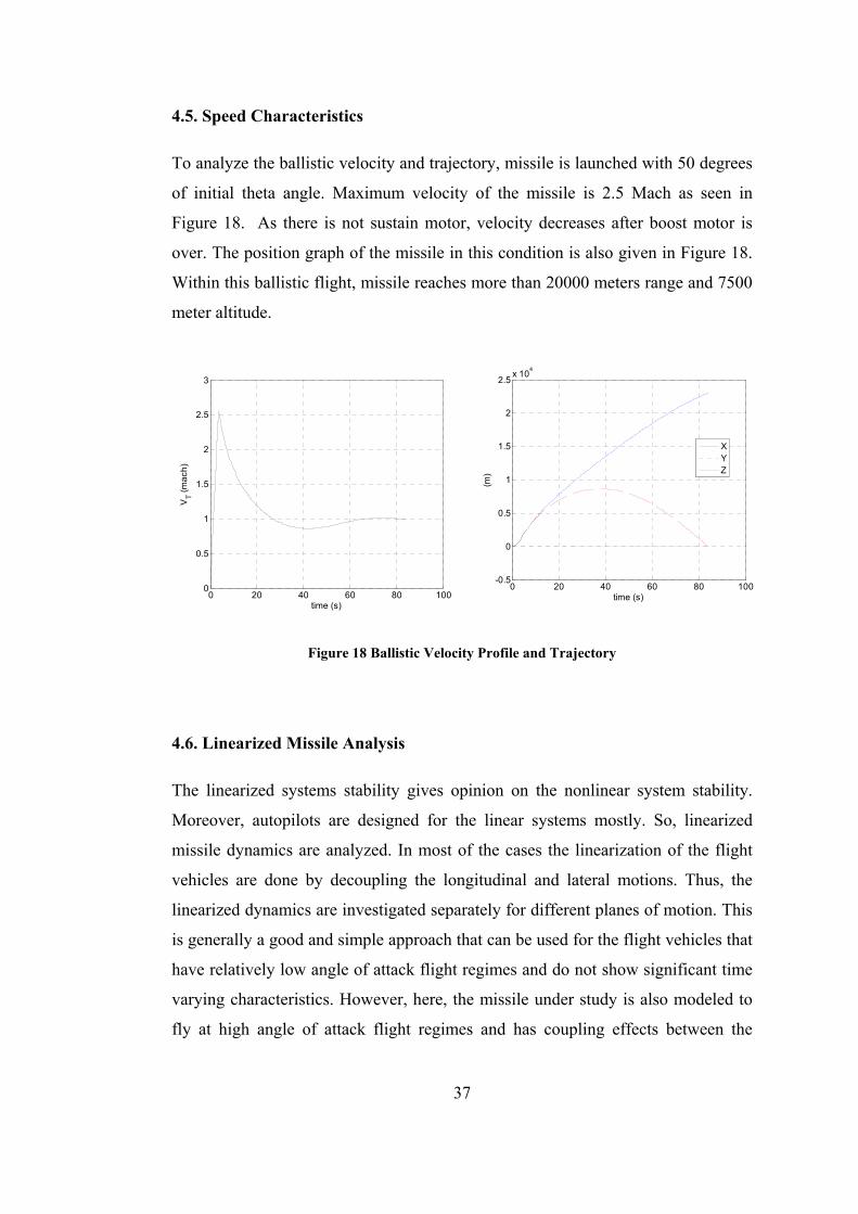
37

4.5. Speed Characteristics

To analyze the ballistic velocity and trajectory, missile is launched with 50 degrees

of initial theta angle. Maximum velocity of the missile is 2.5 Mach as seen in

Figure 18. As there is not sustain motor, velocity decreases after boost motor is

over. The position graph of the missile in this condition is also given in Figure 18.

Within this ballistic flight, missile reaches more than 20000 meters range and 7500

meter altitude.

0 20 40 60 80 1000

0.5

1

1.5

2

2.5

3

time (s)

VT (m

ach)

0 20 40 60 80 100-0.5

0

0.5

1

1.5

2

2.5x 104

time (s)

(m)

XYZ

Figure 18 Ballistic Velocity Profile and Trajectory

4.6. Linearized Missile Analysis

The linearized systems stability gives opinion on the nonlinear system stability.

Moreover, autopilots are designed for the linear systems mostly. So, linearized

missile dynamics are analyzed. In most of the cases the linearization of the flight

vehicles are done by decoupling the longitudinal and lateral motions. Thus, the

linearized dynamics are investigated separately for different planes of motion. This

is generally a good and simple approach that can be used for the flight vehicles that

have relatively low angle of attack flight regimes and do not show significant time

varying characteristics. However, here, the missile under study is also modeled to

fly at high angle of attack flight regimes and has coupling effects between the

38

planes of motion it is necessary to carry out the linearization coupled in both planes

of motion.

In this study the linearization of the nonlinear missile dynamics is done especially

for vertical launch, including the thrust, and the vertical climb, after the engine

burn-out, phases and the controls are locked. Thus, the trim flight conditions are

chosen as

0α β= =

0p q r s= = =

0a e r T e T rδ δ δ δ δ= = = = =

90θ = .

θ is given for visualization purposes, it is not related with Euler angle singularity.

Hence, the linear dynamics can be represented in the state space form. The

aerodynamic and the thrust vectoring surface deflections are the control inputs

( u uΔ = ) and all of the flight variables are the outputs ( y xΔ = Δ ) of the system:

x A x BuΔ = Δ + (4.1)

Here, A is system matrix, B is control matrix and u vector represents thrust vector

control and aerodynamic control inputs and the states are velocity, alpha, beta, roll,

pitch and yaw rates as given;

[ ]Tx U p q rα β φ θΔ = Δ Δ and [ ]T a e r T e T ru δ δ δ δ δ= . It shall be noted that, except UΔ and θΔ , Δ sign is not used for other state

variables for which the trim conditions are taken to be zero, i.e. the deviations from

the trim conditions are equal to the values of the states themselves.

39

Linearization is done for two phases. Missile is vertically launched and a

linearization time interval is decided as 20 seconds. The first 3.5 seconds of the

vertical flight is defined as phase 1, and there is thrust in this phase. In the first

phase, mass, inertia, velocity, center of gravity is changing with respect to time.

The second phase is where there is no thrust. Mass, center of gravity and inertia is

constant; the only changing missile parameter is its velocity. Both of the

linearization conditions for Phase I and II are given in Table 3 and Table 4.

Table 3 Phase I Linearization Parameters

Time (s) Altitude (m) Velocity (Mach) Dynamic Pressure (kg/m3)

0.3 11 0.21 3230

0.65 52 0.47 1610

1.01 126 0.74 38770

1.36 232 1.01 70760

1.72 370 1.27 110530

2.07 540 1.53 156710

2.43 739 1.79 208060

2.78 969 2.04 262860

3.14 1227 2.28 319300

3.5 1514 2.52 375930

40

Table 4 Phase 2 Linearization Parameters

Time (s) Altitude (m) Velocity (Mach) Dynamic Pressure (kg/m3)

4 1929 2.44 335170

5.77 3276 2.16 22123

7.55 4462 1.95 155240

9.33 5529 1.79 113590

11.11 6502 1.66 85490

12.88 7395 1.55 65680

14.66 8222 1.45 51230

16.44 8989 1.36 40390

18.22 9702 1.28 32090

20 10367 1.21 25710

After linearization process, stability analysis of the system is carried on. Eigen

values of A are seen in Figure 19. It has two parts, one is the thrust phase and the

other part is when there is no thrust force. In phase II, as the velocity decreases

immediately, the poles of the system approaches to the imaginary axes. In Table 4,

the last value of the velocity is 1.21 mach which means the linearization process is

being done for less 1.21 Mach. However, missile has to hit the target before its

velocity decreases to critical values with respect to the target. Although analysis for

lower velocity profile is not shown, it is clear that missile stability is decreasing

parallel to its velocity.

41

-4 -3 -2 -1 0-25

-20

-15

-10

-5

0

5

10

15

20

25Thrust Phase

Re

Im

-3 -2 -1 0-25

-20

-15

-10

-5

0

5

10

15

20

25Aerodynamic Phase

Re

Im

Figure 19 Eigen Values of Thrust (a) and Aerodynamic (b) Phases

Here, a state space representation at Mach = 0.27, altitude = 52 meter with two

control inputs is given. As it is seen, cross coupling terms depending on the angle

of attacks is included in linear equations. More state space representations are

presented at [34].

(a) (b)

42

-2.91 0.211e-3 0 0.997 00.211e-3 -2.91 0 0 0.9970.77 e-1 0.77e-1 -0.571 0 0

-12 -0.49e-2 0 -0.216 0 -0.49e-2 12 0 0 -0.216

0 0.089 00 0 0.089

-148 0 00 1

p pq qr r

α αβ β⎡ ⎤ ⎡ ⎤ ⎡ ⎤⎢ ⎥ ⎢ ⎥ ⎢ ⎥−⎢ ⎥ ⎢ ⎥ ⎢ ⎥⎢ ⎥ ⎢ ⎥ ⎢ ⎥= +⎢ ⎥ ⎢ ⎥ ⎢ ⎥⎢ ⎥ ⎢ ⎥ ⎢ ⎥⎢ ⎥ ⎢ ⎥ ⎢ ⎥⎣ ⎦ ⎣ ⎦ ⎣ ⎦

−

−

2.76 00 2.760 0

0.6 0 342 00 0 10.6 0 342

aTe

AeTr

Ar

δδ

δδ

δ

−⎡ ⎤ ⎡ ⎤⎢ ⎥ ⎢ ⎥⎡ ⎤⎢ ⎥ ⎢ ⎥ ⎡ ⎤⎢ ⎥⎢ ⎥ ⎢ ⎥+ ⎢ ⎥⎢ ⎥⎢ ⎥ ⎢ ⎥ ⎣ ⎦⎢ ⎥ −⎣ ⎦⎢ ⎥ ⎢ ⎥⎢ ⎥ ⎢ ⎥⎣ ⎦ ⎣ ⎦

(4.2)

Afterwards, nonlinear and linear system comparison is carried on. During the

comparison it is a very important task to schedule the linear dynamics with respect

to desired flight parameters. In general, the scheduling is done with respect to the

dominant flight parameters that are changing very rapidly when compared to the

other ones in such a way that they affect the coefficients of the linear and also

nonlinear system. A frequently used scheduling method, in missile flight dynamics

linearization, is carrying out the scheduling with respect to Mach number.

However, in the first phase velocity is changing with respect to time. Moreover,

center of gravity, inertia and mass is changing with respect to time. So, first phase

is scheduled with respect to time. Velocity scheduling is applied for the second

phase. Then, a deflection command set is applied for both of the phases and

nonlinear simulation. The angle of attack and pitch rate responses of the two

systems are shown in Figure 20. As seen, for a 1 degree of deflection of jet vanes

and tail fins, the systems’ responses are very close which claims the linearization is

approximately true.

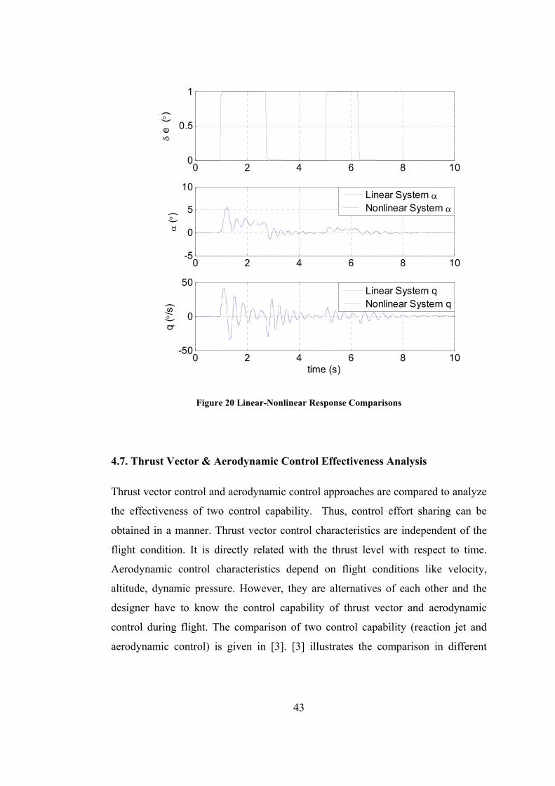
43

0 2 4 6 8 100

0.5

1

δ e ( °

)

0 2 4 6 8 10-5

0

5

10α

( °)

Linear System αNonlinear System α

0 2 4 6 8 10-50

0

50

time (s)

q ( °

/s)

Linear System qNonlinear System q

Figure 20 Linear-Nonlinear Response Comparisons

4.7. Thrust Vector & Aerodynamic Control Effectiveness Analysis

Thrust vector control and aerodynamic control approaches are compared to analyze

the effectiveness of two control capability. Thus, control effort sharing can be

obtained in a manner. Thrust vector control characteristics are independent of the

flight condition. It is directly related with the thrust level with respect to time.

Aerodynamic control characteristics depend on flight conditions like velocity,

altitude, dynamic pressure. However, they are alternatives of each other and the

designer have to know the control capability of thrust vector and aerodynamic

control during flight. The comparison of two control capability (reaction jet and

aerodynamic control) is given in [3]. [3] illustrates the comparison in different

44

altitudes. Here, it is preferred to make comparison during vertical launch which is

the main property of the missile.

As defined in [34] a state space model for the missile dynamics can be written as

A A T Tx Ax B u B u= + + (4.3)

where aero and thrust vector control inputs enter the system dynamic through TB

and AB matrices. Control effectiveness can be analyzed by computing the ratio of

these matrices throughout the flight envelope. So, the ratio of control inputs

(aerodynamic and thrust vector control) for angle of attack dynamics; and the flight

envelope is illustrated in Figure 21 as an example. As seen in Figure 21, thrust

vector control is more effective than aerodynamic control where velocity and

dynamic pressure are low. As velocity increases, so the dynamic pressure, the ratio

of the control capability decreases. After 1 Mach, control effectiveness is close to 1

which means aerodynamic control is as effective as thrust vector control. In the

end, where thrust is over, thrust vector control is no more available.

45

0 1 2 30

10

20

30

40

50

60Control Effectiveness

Mach

thr/a

ero

0 1 2 30

2000

4000

6000

8000

10000

12000

14000

16000

18000Flight Envelope

Mach

Alti

tude

(m)

Figure 21 Control Effectiveness of Thrust/Aero Control

The problem is that if there is a mechanical connection between these control

surfaces which means they are actuated by the same actuator system, what the ratio

should be or what advantages of actuating the control surfaces separately are. If this

problem is formulated, the overall state equations can be defined as where AB is

aerodynamic control, TB is thrust vector control inputs. If hybrid control is selected

the state equation can be written such as:

A Tx Ax ( B KB )u= + + (4.4)

And the control input is then:

[ ]Ta e ru δ δ δ= where /e Ae Te Kδ δ δ= = and /r Ar Tr Kδ δ δ= = .

46

The point is deciding to actuate the control surfaces (jet vanes and tail fins)

separately or coupled. As a design procedure, it can be decided to actuate control

surfaces separately. However, in literature, missiles which use tail fins and jet

vanes as control surfaces usually chose coupled actuating systems which is called

hybrid control [13], [14] and [47]. Figure 22 shows the hybrid control actuator of

ESSM missile; here both jet vanes and tail fins are actuated by one

electromechanical actuator.

Figure 22 ESSM TV-Aero Control Hybrid Control Actuator [5]

As both of the control surfaces are at the end of the missile, these control surfaces

are coupled to each other in order to packaging and power advantages. So coupled

usage of the control surfaces is preferred. This ratio is also a design period result. It

can be optimized with the known parameters like, control effectiveness, mechanical

design parameters, limited space, power needing, mass for actuator etc. which is

another study subject. However, as this study is not focused on optimization of the

coupling ratio, for the sake of simplicity, the ratio is taken where the control inputs

relatively same maneuvers, it is preferred 0.87 which means thrust vector control

surfaces are less actuated. This will also minimize the amount the thrust loss;

however in the thesis thrust loss is not a lot, less than % 1; however in real

applications thrust loss is more than % 1.

47

CHAPTER 5

AUTOPILOT DESIGN

There are nonlinear controller design methods for agile, highly varying dynamical

systems. [48] discusses control strategies for high angle of attack missiles, and

presents comparison of linear and nonlinear control approaches. [49] is an autopilot

design study for IRIS-T missile which is based on robust control theory. [50] is

similar to the study in [49]. [4] is a sliding mode control strategy for air-to-air

missiles. [51] is a brief application of classical autopilot structures working on high

angle of attack. [52] and [53] are studies of autopilot designs on adaptive control

theory. [52] discusses the controller design problem of the same application with a

similar approach. It considers some periods as time varying systems and suggests a

solution for this kind of highly varying dynamic systems. [54] is a master thesis on

bang – bang controllers for VLSAM; however it is a very brief study without any

detailed analysis. As seen, it is possible to find many different autopilot structures.

However, before high level autopilot structures, it is decided to understand and

analyze the capability of classical approaches and gain scheduling method in such

systems and it is decided to start autopilot design with classical approaches.

Autopilot designs are been considered in the scope of existing feedback sensors on

missiles such as gyros and accelerometers. Hence, body rates, angle and

acceleration autopilots are studied on. Autopilots are designed for the linearized

systems. Then, the autopilot structures are implemented into the nonlinear

mathematical model and the gains are scheduled which is mostly done practically.

The autopilots are activated after 0.2 seconds from launch, in order to be sure that

48

missile is at least at 5 meters height from the launcher. Missile is accelerated for

3.5 seconds and its velocity changes from 0 to 900 m/s (2.5 Mach) in 3.5 seconds.

After 3.5 seconds, its velocity is decreasing rapidly. Moreover center of gravity,

mass and inertia are also changing with respect to time, but constant after boost

motor burns.

Due to the rapid change in velocity and dynamic pressure, plant parameters change

rapidly. Beside these changes, desired angle of attack regions are also too wide as it

is VLSAM. Consequently, autopilots must be as robust as possible towards these

changes. As high angle of attack maneuvers are studied, cross couplings and

nonlinear behaviors also occur [51].

As a first step, cross couplings between the two motions can be considered as

disturbances and the autopilot should be capable of reducing the sensitivity of the

missile to those disturbances for an acceptable level. Outputs of autopilot module

are the desired deflection commands which will be realized by tail and jet vane

deflections. These commands will be the input to the missile dynamics.

In the following part, body rate, angle, and acceleration autopilots are presented.

After each autopilot design is completed, its performance is tested in the nonlinear

simulation environment that includes nonlinear autopilot module (formed by gain

scheduling method) and nonlinear missile model. Autopilots are tested with

reference command signals.

5.1. Pitch Autopilot Design

In the derivation of autopilot model that will be used within the application of

control system, equations of motion should also be linearized around equilibrium

flight (trim) points. As mentioned in the linear missile analysis, because of cross

coupling dynamics, agile missile dynamics are not decoupled for pitch, yaw and

roll planes. However, if the coupling terms are taken into account as disturbance,

some of standard approaches (short period approximation) can be applied. In this

section, a linearization procedure is performed. First of all, for a skid-to-turn

49

missile, aiming to have no roll rate and keeping roll angle at a constant steady state

value, and also decoupling pitch and roll-yaw plane state equations result in taking

roll rate approximately zero.

In short period approach, one of the main assumptions is missile’s velocity is not

changing. However, in boost phase, missile is highly accelerating and the

assumption is not completely true [55]. As control is critical in boost phase where it

lasts for 3.5 seconds, velocity change has to be taken into account. If derivation of

angle of attack is examined, rate of change of the velocity (acceleration of the

missile) is seen to be included in the equations (4.5) and (4.6).

wu wu w uu uu

α α−= = −2 (4.5)

It is assumed that u and u are constant at the linearization instant so the Eq. (5.1)

becomes:

w U Uα α= + (4.6)

Using the linearized forms of aerodynamic coefficients given in the previous

section, linear dynamic equations are obtained as follows:

2q e

xm m m e

yy yy yy

TlQ S d Q S ddq C C q C KI U I Iα δ

α δ⎛ ⎞⎛ ⎞

= + + −⎜ ⎟⎜ ⎟ ⎜ ⎟⎝ ⎠ ⎝ ⎠ (4.7)

21 q

e

z z

z e

Q S Q S dC U C U qm m U

U Q S TC Km m

α

δ

αα

δ

⎛ ⎞⎛ ⎞⎛ ⎞− + +⎜ ⎟⎜ ⎟⎜ ⎟⎝ ⎠ ⎝ ⎠⎜ ⎟= ⎜ ⎟⎛ ⎞⎜ ⎟+ −⎜ ⎟⎜ ⎟⎝ ⎠⎝ ⎠

(4.8)

As a simplification, equations (7.6)-(7.7) can be stated as

eq eq M M q Mα δα δ= + + (4.9)

50

( ) ( 1)eq e

UZ Z ZUα δα α δ= − + + + (4.10)

The stability derivatives used in the equations (4.9) and (4.10) are:

2

2 q

e e

m q myy yy

tm

yy yy

Q S d Q S dM C , M C ,I I U

TlQ S d M C KI I

α

δ δ

α = =

= + (4.11)

22 q

e e

Z q Z

z

Q S Q SdZ C , Z C ,mU mUQ S T Z C KmU mU

α

δ

α

δ

= =

= + (4.12)

where K is the hybrid control ratio. State space representation is then:

1

eq

eq

U ZZ ZA BU

MM M

δα

δα

⎡ ⎤− + ⎡ ⎤⎢ ⎥= = ⎢ ⎥⎢ ⎥ ⎣ ⎦⎢ ⎥⎣ ⎦

(4.13)

In the following section controller design process will be presented. Dynamical

system analyses are critical for understanding of all systems. Thus, before

controller design, system dynamics must be understood well. Firstly, change in

parameters of A and B matrices are examined. As seen in Figure 23 and Figure 24,

stability derivatives change rapidly within the time of boost phase. Especially

changes of Mα and eMδ are so drastic. Moreover, trend of the changes are not

linear; it is seen that around the time 1.5 second there is a peak change. This change

can be related with transonic region aerodynamic characteristics. After 1.5th

second, parameters change with another tendency which is because of transonic

region behavior [51]. As seen in Figure 23 and Figure 24, most of the coefficients

reach a peak value at 1.5th second where velocity is 1.15 Mach.

51

0 0.5 1 1.5 2 2.5 3 3.5-4

-3

-2

-1

A11

0 0.5 1 1.5 2 2.5 3 3.5-600

-400

-200

0

A21

0 0.5 1 1.5 2 2.5 3 3.5-2

-1.5

-1

-0.5

0

time (s)

A22

Figure 23 State Equations’ Parameter Variations

0 0.5 1 1.5 2 2.5 3 3.5-3.5

-3

-2.5

-2

-1.5

-1

-0.5

0 0.5 1 1.5 2 2.5 3 3.5-800

-700

-600

-500

-400

-300

time (s)

B1

B2

Figure 24 Control Parameters’ Variations

52

In addition to varying parameter analyses, pitch rate natural frequency and damping

coefficient changes are analyzed. Firstly, the transfer function of pitch rate with

respect to hybrid elevator deflection (thrust vector and aerodynamic control where

hybrid control ratio is 0.87) is obtained which is given in Eq. (4.14) and (4.15):

2

( )( )( ) ( ) ( )

e e e

e q q q

M s Z U U M M Zq ss s s M Z U U Z U U M M Z M

δ α δ α δ

α α α αδ− − +

=− + − + − − −

(4.14)

( )

( ) , 2

qn q q

n

M Z U Uw Z U U M M Z M

wα

α α α ξ+ −

= − − − = (4.15)

Then, natural frequency and the damping coefficient of the system for the boost

phase are given in Figure 25 and Figure 26. One of the main issues in natural

frequency and damping coefficient change is, as velocity increases natural

frequency of the system increases with similar trend of the velocity profile.

Damping coefficient decreases highly when velocity increases. Figure 27 shows the

DC gain of the system during the boost phase. In the early stages of the flight time,

its value is high. Immediately after the initial phase, its value decreases rapidly like

an exponential function. Figure 28 is the pole zero map of the pitch rate dynamics.

It can be examined better with the location of the poles and zeros. The same

transonic region system behavior can also be seen in pole-zero map. This behavior

was not recognized so clearly when boost phase is divided into 10 discrete time

steps ( 0.35tΔ = s). It is recognized during the autopilot design process. Although

the linear controllers’ performance was good, linear time varying responses were

not as good as expected. In order to analyze poles and zeros in more details, boost

phase is divided into 40 discrete time intervals ( 0.0875tΔ = s) and controllers are

designed for 40 plants.

53

0 0.5 1 1.5 2 2.5 3 3.50

5

10

15

20

25

time (s)

wn (r

ad/s

)

Figure 25 Natural Frequency of Pitch Rate Dynamics

0 0.5 1 1.5 2 2.5 3 3.50

0.1

0.2

0.3

0.4

0.5

0.6

0.7

time (s)

ζ

Figure 26 Damping Coefficient for Pitch Rate Dynamics

54

0 0.5 1 1.5 2 2.5 3 3.5-20

0

20

40

60

80

100

120

140

time (s)

DC

gai

n

Figure 27 DC Gain of Pitch Rate Dynamics

-3 -2.5 -2 -1.5 -1 -0.5 0-25

-20

-15

-10

-5

0

5

10

15

20

25Pole-Zero Map

Real Axis

Imag

inar

y Ax

is

Figure 28 Pole Zero Map of Pitch Rate Dynamics

55

5.1.1. Pitch Rate Autopilot Design I

In this section, pitch rate is controlled with classical pitch rate controller. This type

of controller is widely used in missile autopilots. Structure of the controller is given

in Figure 29. Controller includes a zero and an integrator to inhibit steady state

error. The state space representation and the parameters of the matrices are given in

the previous section, so transfer function representation is not given again.

Figure 29 Pitch Rate Controller Structure I

It is obvious that the dominant pole placement technique cannot be applied with

two free parameters. So, the parameters can be determined by time or frequency

characteristics. Zeros of the controllers are placed in root locus and performance is

examined for all frozen linear plants. The gains of the autopilot are given in Table

5. The responses of 10 linear time invariant plants and the deflections are seen in

Figure 30. Settling time is less than 1 second in general and system behavior is like

a first order system. These gains are scheduled with respect to time in the nonlinear

simulation. The nonlinear simulation response and deflection is given in Figure 31.

In all nonlinear simulation, nonlinear first order control actuator dynamics (w:300

rad/s) is included.

- ( )( )e

q ssδ

1 ( )iK s ws+

-

56

Table 5 Gains of the Controller for 10 LTI Systems at Δt=0.35s

K1 wi

LTI 1 0.168 1.15

LTI 2 0.26 2.185

LTI 3 0.364 2.898

LTI 4 0.4 4.14

LTI 5 0.46 2.76

LTI 6 0.48 3.45

LTI 7 0.44 3.68

LTI 8 0.48 3.91

LTI 9 0.5 4.14

LTI 10 0.52 4.37

0 0.5 1 1.5 2 2.50

0.5

1

q ( °

/s)

0 0.5 1 1.5 2 2.5

-0.3

-0.2

-0.1

0

time (s)

δ e( °)

first system

last system

Figure 30 LTI Plants and Deflections I

57

0 0.5 1 1.5 2 2.5 3 3.5-10

-5

0

5

10

q ( °

/s)

0 0.5 1 1.5 2 2.5 3 3.5-2

-1

0

1

2

time (s)

δ e ( °)

referenceresponse

Figure 31 Pitch Rate Response and Deflection I (Nonlinear Simulation)

5.1.2. Pitch Rate Autopilot Design II

To analyze another control structure for the pitch rate dynamics, autopilot structure

with state feedback is studied on. The A and B matrices of the pitch dynamics are

given for the boost phase in Figure 23 and Figure 24. In this design procedure, a

state feedback and feed forward gain is preferred. One of the desired poles is

placed at the zero of the open loop system to improve the transient response and the

other pole is placed at 1.25 times of nw (Figure 25) of the linearized systems

because of actuator time constant. The design procedure is applied to 40 linear time

invariant plants (Δt=0.0875 s). The feed forward gain and state feedback gains are

illustrated in Figure 32 and Figure 33. The responses of each plant and the

deflections are seen in Figure 34. The responses of the LTI plants are quite well.

However, when the plants are changed with respect to the linearized time schedule,

response of the plant (linear time varying plant) varies. Interestingly, step response

is not as good as LTI responses, see Figure 35. The second step of performance

analysis of the design is using the autopilot in nonlinear simulation. As the feed-

58

forward gain is used in autopilot structure, the response will get worse whenever

system is away from the linearization points. Figure 36 is the comparison of LTV

plant and nonlinear plant with an approximately symmetric signal. Autopilot

response is acceptable. But, it is hard to say it for the response in Figure 37. For

related deflection angles, see Figure 38. This result directs a designer to find

another autopilot structure.

0 5 10 15 20 25 30 35 400.01

0.015

0.02

0.025

0.03

0.035

0.04

Linearized System Number

Feed

forw

ard

Gai

n

Figure 32 Feedforward Gain for the Linearized Systems

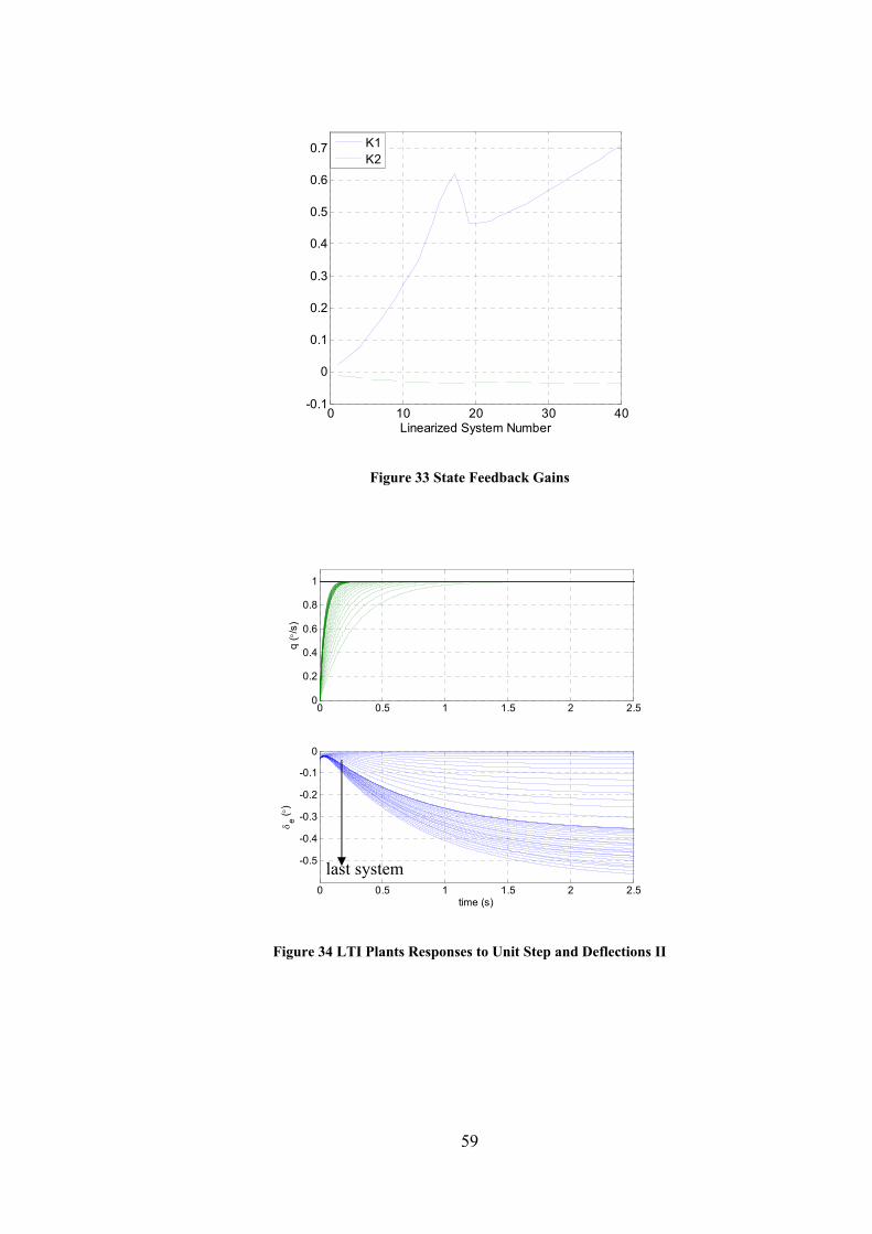
59

0 10 20 30 40-0.1

0

0.1

0.2

0.3

0.4

0.5

0.6

0.7


K1K2

Figure 33 State Feedback Gains

0 0.5 1 1.5 2 2.50

0.2

0.4

0.6

0.8

1

q ( °

/s)

0 0.5 1 1.5 2 2.5

-0.5

-0.4

-0.3

-0.2

-0.1

0

time (s)

δ e ( °)

Figure 34 LTI Plants Responses to Unit Step and Deflections II

last system

60

0 0.5 1 1.5 2 2.50

0.5

1

q ( °

/s)

0 0.5 1 1.5 2 2.5 3 3.5-0.8

-0.6

-0.4

-0.2

0

time (s)

δ e ( °)

referenceresponse

Figure 35 LTV Plants Response and Deflection II

0 0.5 1 1.5 2 2.5 3 3.5-30

-20

-10

0

10

20

30

time (s)

q ( °

/s)

referencenonlinear res.ltv res.

Figure 36 Autopilot Response to Symmetric Reference Input

61

0 0.5 1 1.5 2 2.5 3 3.5-30

-20

-10

0

10

20

30

40

50

time (s)

q ( °

/s)

referencenonlinear res.ltv res.

Figure 37 Autopilot Response to non-Symmetric Reference Input

0 0.5 1 1.5 2 2.5 3 3.5-1

0

1

2

3

4

5

6

7

time (s)

δ e ( °)

nonlinear δeltv δe

Figure 38 Deflection Angles

62

5.1.3. Pitch Rate Autopilot Design III

As controlled pitch rate dynamics is a type-one system and zeros of the system

affects the transient response, practical suboptimal tracker method is studied on. In

this section, practical suboptimal control structure with application to pitch rate

dynamics will be held. The mentioned control structure and the necessity behind

integrating the error is briefly described at [56].

By integrating the error dynamics to the system dynamics, the new state space

representation is obtained as:

x A x B

u r, y C xC Iξξ

•

•

⎡ ⎤ ⎡ ⎤ ⎡ ⎤ ⎡ ⎤ ⎡ ⎤⎢ ⎥ = + + =⎢ ⎥ ⎢ ⎥ ⎢ ⎥ ⎢ ⎥⎢ ⎥ −⎣ ⎦ ⎣ ⎦ ⎣ ⎦ ⎣ ⎦⎣ ⎦

0 00 0

(4.16)

where

comq qξ = − (4.17)

and the control input is

[ ]u K 2 K3 x K1ξ= − + (4.18)

Overall gain matrix which can be chosen with pole placement method is:

[ ]TK K 2 K3 K1= − (4.19)

For the boost phase of the system, one of the poles is placed at the zero of the

system. The other poles are placed to the natural frequency and 1.3 times of the

natural frequency of the linear systems. The state feedback gains are illustrated in

Figure 39. Closed loop responses of linear systems and the elevation commands are

illustrated in Figure 40. The slowest one of the linear systems (0.3 seconds after

vertical launch) settles down before 2 seconds and the maximum deflection angle is

0.6º. To analyze the performance of the overall system during the boost phase,

63

linear time varying model is used with the given control structure. The controller’s

parameters are also changed and interpolated with respect to time. In this structure

which will be the behavior of vertical launch system, the response and the

deflection of the system is given in Figure 41. As seen, the step response of the

system is not the like the ones given in Figure 40. This is a direct consequence of

dealing with a highly varying system result whose parameter changes are given in

Figure 23 and Figure 24, [52]. In order to analyze the final performance of the

controller, controller structure is embedded into the nonlinear simulation and a

reference input is given to the nonlinear system. The reference input, LTV and

nonlinear system responses are given in Figure 42 and the deflections of LTV and

nonlinear system is in Figure 43. It is clearly seen that the nonlinear response is not

as satisfactory as expected which shows that it is not possible to have the desired

responses with pure gain scheduling.

0 10 20 30 40-0.1

0

0.1

0.2

0.3

0.4

0.5

0.6

0.7


K1K2K3

Figure 39 Gains of the Controller

64

0 0.5 1 1.5 2 2.5 30

0.5

1

q ( °

/s)

0 0.5 1 1.5 2 2.5 3

-0.6

-0.4

-0.2

0

time (s)

δ e ( °)

Figure 40 LTI Responses and Deflection Angles III

0 1 2 3 4 50

0.5

1

1.5

q ( °

/s)

0 1 2 3 4 5

-0.6

-0.4

-0.2

0

time (s)

δ e ( °)

Figure 41 LTV Response and Deflection Command III

last system

65

0 0.5 1 1.5 2 2.5 3 3.5

-60

-50

-40

-30

-20

-10

0

10

20

30

40

time (s)

q ( °

/s)

referencenonlinear res.ltv response

Figure 42 Nonlinear and LTV Responses

0 0.5 1 1.5 2 2.5 3 3.5-5

0

5

10

15

20

time (s)

δ e ( °)

nonlinear ltv

Figure 43 Nonlinear and LTV Systems Deflections

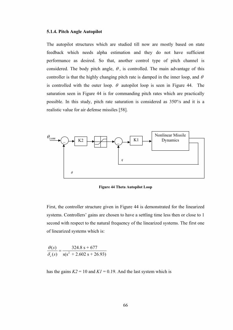
66

5.1.4. Pitch Angle Autopilot

The autopilot structures which are studied till now are mostly based on state

feedback which needs alpha estimation and they do not have sufficient

performance as desired. So that, another control type of pitch channel is

considered. The body pitch angle, θ , is controlled. The main advantage of this

controller is that the highly changing pitch rate is damped in the inner loop, and θ

is controlled with the outer loop. θ autopilot loop is seen in Figure 44. The

saturation seen in Figure 44 is for commanding pitch rates which are practically

possible. In this study, pitch rate saturation is considered as 350º/s and it is a

realistic value for air defense missiles [58].

Figure 44 Theta Autopilot Loop

First, the controller structure given in Figure 44 is demonstrated for the linearized

systems. Controllers’ gains are chosen to have a settling time less then or close to 1

second with respect to the natural frequency of the linearized systems. The first one

of linearized systems which is:

2

( ) 324.8 s + 677( ) s(s + 2.602 s + 26.93)e

ss

θδ

=

has the gains K2 = 10 and K1 = 0.19. And the last system which is

Nonlinear Missile Dynamics

K2 comθ

θ

q

_ _ K1

67

2

( ) 761.5 s + 917.5( ) s(s + 3.12 s + 543.4)e

ss

θδ

=

has the gains K2 = 37 and K1 = 0.58. The two linearized systems’ response to a

step input can be seen in Figure 45. Afterwards, the controller is embedded into the

nonlinear simulation and scheduled with respect to time. Desired command and

response with deflection is seen in Figure 46. In this scenario, missile is vertically

launched and after it reaches 5m altitude, and control starts. For one second, zero

command is sent to turnover the missile. Then this command is changed to pitch up

till 2.5 seconds and finally for the last second command is directionally reversed.

As seen, the turnover maneuver is successfully accomplished. The autopilot

performance to turnover the pitch up - pitch down maneuvers are quite well within

the varying parameters profile given in Figure 47 where angle of attack is changing

between 0 and 60 degrees, velocity is accelerated from 0 to 2.5 Mach during 3.5

seconds.

0 0.5 1 1.5 2 2.5 30

0.2

0.4

0.6

0.8

1

time (s)

θ ( °

)

lti system 1lti system 40

Figure 45 LTI Responses

68

0 0.5 1 1.5 2 2.5 3 3.5

0

20

40

60

80

θ ( °

)

0 0.5 1 1.5 2 2.5 3 3.5-0.4

-0.2

0

0.2

0.4

time (s)

δ e (rad

)

θ commandθ response

Figure 46 Nonlinear Simulation Response and Deflection

0 200 400 600 800 1000 12000

200

400

H (m

)

X (m)

0 0.5 1 1.5 2 2.5 3 3.5-60-40-20

020

α ( °

)

0 0.5 1 1.5 2 2.5 3 3.50123

VT (M

ach)

0 0.5 1 1.5 2 2.5 3 3.5-400

-200

0

q ( °

/s)

time (s)

Figure 47 Altitude, Angle of Attack, Velocity, Pitch Rate During the Maneuver

69

5.1.4.1. Missile Turn Over Capability Analysis with Angle Autopilots

In an effort to determine the capability of hybrid controlled VLSAM, 3 scenarios

are formed. In all of the scenarios, missile starts the turnover maneuver from

different altitudes. In each turnover altitude, theta commands are applied until 3.5

seconds. In the first scenario, θ starts from 90 degrees, a θ command of 45

degrees is applied till the boost motor is over. Figure 48 shows the variation of

altitude and downrange of missile during 45 degrees of continuous theta command.

In the second scenario, θ starts from 90 degrees, and then a θ command of 0

degrees is applied till the boost motor is over. Control commands are started to be

sent at different altitudes. The minimum turnover altitude is more than 150 meters

and the maximum turnover altitude is more than 400 meters as seen in Figure 49.

In the third scenario, a θ command of -45 degrees is executed. Figure 50 shows the

minimum downrange with minimum altitude capability of the missile. If the

missile starts the turnover maneuver at 5 meters altitude, it can approach 200

meters range within an altitude of 50 meters. But if, it starts turning at 100 meters

altitude, it can approach 500-600 meters downrange within an altitude of about 270

meters.

70

0 200 400 600 800 10000

200

400

600

800

1000

1200

H (m

)

X (m)

h=5mh=25mh=50mh=75mh=100mh=200mh=400m

Figure 48 X-H Graph at Fθ = 45º wrt. to Various Initial Turnover Altitudes

0 200 400 600 800 1000 1200 14000

50

100

150

200

250

300

350

400

450

H (m

)

X (m)

h=100mh=75mh=50mh=25mh=5m

Figure 49 X-H Graph at Fθ = 0º wrt. Various Initial Turnover Altitudes

71

0 100 200 300 400 500 6000

50

100

150

200

250

300

H (m

)

X (m)

h=5mh=25mh=50mh=75mh=100m

Figure 50 X-H Graph at Fθ =- 45º wrt. Various Initial Turnover Altitudes

5.2. Roll Autopilot Design

Using the linearized forms of aerodynamic coefficients as in the previous section,

linear dynamic equations for the roll plane are obtained as follows:

2 ap

l l l alxx

Q S d dp C C C p CI Uα β δ

α β δ⎛ ⎞

= + + +⎜ ⎟⎝ ⎠

(4.20)

pφ = (4.21)

In equations (7.8)-(7.9), the stability derivatives used are:

2

2 p

a a

p l lxx xx

l lxx xx

Q Sd Q S dL C , L C ,I U I

Q S d Q S dL C , L CI I

β

α δ

β

α δ

= =

= = (4.22)

72

xx p aI p L p L a L Lδ α βδ α β= + + + (4.23)

If the terms connected with attack angles α and β are treated as disturbances the

roll rate derivative can be rewritten as:

xx p aI p L p L aδ δ= + (4.24)

where transfer function is expressed as:

( )( )

a

a xx p

Lp ss sI L

δ

δ=

− (4.25)

Pole of the transfer function in equation (4.25) with respect to mach and altitude for

thrust phase is given in Figure 51. Rise in velocity directly results decrease in time

constant.

Pole-Zero Map

Real Axis

Imag

inar

y Ax

is

-3.5 -3 -2.5 -2 -1.5 -1 -0.5 0-1

-0.8

-0.6

-0.4

-0.2

0

0.2

0.4

0.6

0.8

1

machincreases

Figure 51 Pole Zero Map of Roll Channel

73

5.2.1. Roll Angle Autopilot

Roll angle control is performed with the same approach as in the theta control. The

angle of sideslip and attack components are taken into account as disturbances.

Roll commands are desired to be realized as soon as possible within actuator

limitations. Firstly, controller structure given in Figure 52 is demonstrated for the

linearized systems. Controllers gains are chosen to have a settling time changing

from 1 to 5 seconds with respect to the natural frequency of linearized systems. The

first linearized system is:

( ) 49.9 ( ) s(s + 0.402)a

ss

φδ

= .

It has the gains K2 = 0.8 and K1 = 0.02. The last system is

( ) 2810( ) s(s + 3.18)a

ss

φδ

=

having the gains K2 = 2 and K1 = 0.04. The step responses of the first and fortieth

systems are shown in Figure 53. Controller’s gains are updated for all of the

linearized systems. Afterwards, the controller is embedded into the nonlinear

simulation. Desired command, response and deflection are seen in Figure 54.

Figure 52 Roll Angle Control Structure

Nonlinear Missile Dynamics

K2 comφ

φ

p

_ _ K1

74

0 2 4 6 8 100

0.2

0.4

0.6

0.8

1

time (s)

φ ( °

)

system 1system 40

Figure 53 LTI Responses

0 1 2 3 4

-100

-50

0

50

φ ( °

)

0 1 2 3 4-5

0

5

δ a ( °)

time (s)

referenceφ response

Figure 54 Roll Angle and Deflection Angle (nonlinear simulation)

75

5.2.2. Roll Rate Autopilot

In roll plane, another control parameter is the roll rate, p. High angle of attacks’

effects are omitted. So, the same transfer functions without the integrator which are

given in the roll angle autopilot and the pole-zero maps given in Figure 51 are

valid for the roll rate dynamics.

In order to control the roll rate, the controller structure in Figure 55 is applied to the

linearized systems. The controllers for the first and the last linearized boost phase

systems are given below:

10.051 0.02sC

s+

= and 400.023 0.04sC

s+

= .

Step responses of closed loop systems can be seen in Figure 56. Overall settling

time is less than 1.6 seconds. After controllers’ gains are scheduled with respect to

time in the nonlinear simulation environment, a reference command is send to the

roll channel which is given in Figure 57. Both controllers’ response and aileron

deflection command is quite well. Roll angle for the achieved roll rate is also given

in Figure 57.

Figure 55 Roll Rate Controller Structure

( )( )a

p ssδcomp

p

1 2K s Ks+_

76

0 0.5 1 1.5 20

0.2

0.4

0.6

0.8

1

time (s)

p ( °

)

system 1system 40

Figure 56 LTI Responses of Roll Rate Control

Figure 57 Roll Rate Reference and Response with Deflection Angle (Nonlinear)

5.3. Acceleration Autopilot

The autopilot structures till now are planned to be used in the midcourse guidance

phase. However, acceleration autopilot is preferred for the terminal guidance. In

order to use proportional navigation guidance, it will be beneficial to design

77

acceleration autopilot for the phase where pure aerodynamic control surfaces are

used. The state space equation for the pitch plane integrated with actuator dynamics

is:

,

1 00

0 0

e

e

q

q e c

e

UZ Z ZU

q M M M q

α δ

α δ

α αδ

δ δ ωω

⎡ ⎤− +⎢ ⎥⎡ ⎤ ⎡ ⎤ ⎡ ⎤⎢ ⎥⎢ ⎥ ⎢ ⎥ ⎢ ⎥= +⎢ ⎥⎢ ⎥ ⎢ ⎥ ⎢ ⎥⎢ ⎥⎢ ⎥ ⎢ ⎥ ⎢ ⎥−⎣ ⎦ ⎣ ⎦ ⎣ ⎦⎢ ⎥

⎢ ⎥⎣ ⎦

(4.26)

ez ea Z Zα δα δ= + (4.27)

where actuator transfer function is

,

( )( )

e

e c

ss s

δ ωδ ω

=+

(4.28)

that can be written in the state space form as

,( ) ( )e e e csδ ω δ δ= − + (4.29)

To analyze the acceleration dynamics, pole-zero analysis is carried on. Figure 58

shows the pole and zeros of acceleration dynamics. As it is known, in this study,

there is only one boost motor; so that after the boost phase is over velocity

decreases quickly. Decrease in the velocity results a corresponding decrease in the

stability of the acceleration dynamics as seen in Figure 58.

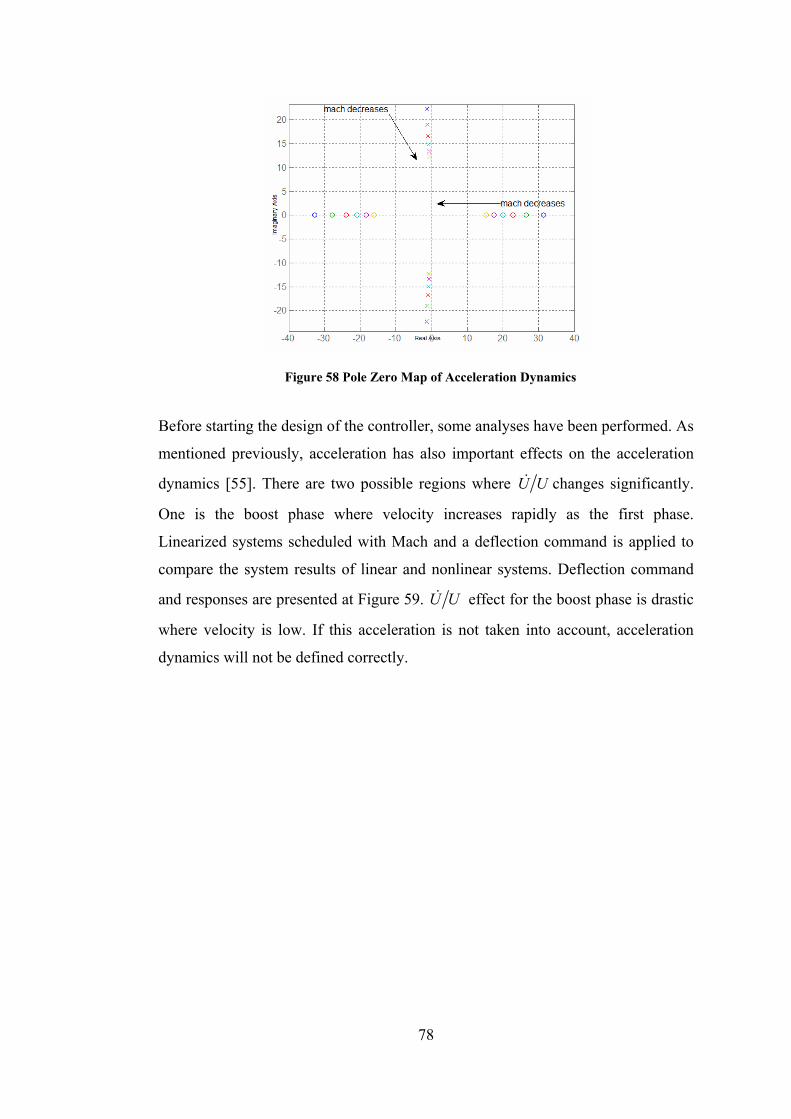
78

Figure 58 Pole Zero Map of Acceleration Dynamics

Before starting the design of the controller, some analyses have been performed. As

mentioned previously, acceleration has also important effects on the acceleration

dynamics [55]. There are two possible regions where U U changes significantly.

One is the boost phase where velocity increases rapidly as the first phase.

Linearized systems scheduled with Mach and a deflection command is applied to

compare the system results of linear and nonlinear systems. Deflection command

and responses are presented at Figure 59. U U effect for the boost phase is drastic

where velocity is low. If this acceleration is not taken into account, acceleration

dynamics will not be defined correctly.

79

0 0.5 1 1.5 2 2.5 3 3.5-150

-100

-50

0

50

100

acce

lera

tion

(m/s2 )

0 0.5 1 1.5 2 2.5 3 3.50

0.2

0.4

0.6

0.8

1

time (s)

δ e ( °)

with udotnonlinearwithout udot

Figure 59 U U Effect on Linear-Nonlinear System Comparison

The second condition where change in U U is the terminal phase where high

acceleration is needed for interception. In the terminal phase, this change has to be

considered if needed. Trim points for the acceleration autopilot are given in Table

6. Acceleration autopilot design depends basically on classical 3 loop autopilot

structure [57] with specified design parameters in Table 7. Structure of the three

loop autopilot is also presented in Figure 60.

Table 6 Trim Points Used for Autopilot Design

Variables Trim Points

Angle of Attack (deg.) 0º

Velocity (Mach)

2.41 2.09 1.87 1.69 1.55

1.43 1.32 1.23

Altitude (m) 1514 1929 3276 4462 5529

6502 7395 8222

Here is a transfer function of acceleration dynamics where velocity is 2.41 Mach

and altitude is 1514 m:

80

2

2( ) 222 302.5 2.542 5( ) 2.66 499.8

z

e

a s s s es s sδ

− − +=

+ +

and

2

2( ) 95.3 74.49 3.425 5( ) 1.445 180.5

z

e

a s s s es s sδ

− − +=

+ +

where velocity is 419 m/s and altitude is 8222 m.

Figure 60 Three Loop Acceleration Autopilot Loop

Designed control structure is applied to linearized systems within the design

criteria are given in Table 7. The controllers’ gains are also given in Table 7 and

they are changing between the given gains given for the first and last linearized

system. Settling time and rise time is decided with respect to linearized systems

natural frequencies and actuator bandwidths. The LTI responses for the linearized

systems are presented in Figure 61. The autopilot structure and the gains are

embedded into the nonlinear simulation and scheduled with velocity to examine its

performance in the nonlinear model. Response to a 0.5 Hz 20 m/sn2 square wave

command is illustrated in Figure 62. The angle of attack change while performing

the reference command is also given in Figure 63. As expected, deflection angle

and angle of attack are increasing in order to achieve the desired acceleration

command because missile’s velocity is decreasing. The changing parameters,

velocity and dynamic pressure, are also exhibited to come to a decision of autopilot

_ _ _

81

performance in Figure 64. As seen, acceleration commands are performed while

velocity and dynamic pressure are changing very rapidly.

Table 7 Design Parameters and Gains

Settling Time (sec) < 1.5

Rise Time (sec) < 0.5

[K1 K2 K3 K4] [ ]0.1119 -0.0119 -20.4 1.035 -

[ ]0.0898 -0.0086 -22.7 1.0125

0 0.5 1 1.5 2 2.5 3-0.2

0

0.2

0.4

0.6

0.8

1

1.2

time (s)

a z(m/s

n2 )

Figure 61 LTI Responses of Closed Loop Systems

82

4 6 8 10 12

-20

0

20

40

a z (m/s

2 )

4 6 8 10 12-5

0

5

10

δ e ( °)

time (s)

referenceresponse

Figure 62 Nonlinear Simulation Response and Deflection Angle

4 6 8 10 12-5

-4

-3

-2

-1

0

1

2

3

4

α ( °

)

time (s)

Figure 63 Angle of Attack During the Nonlinear Simulation

83

4 6 8 10 121

1.5

2

2.5

VT (m

ach)

4 6 8 10 121

2

3

4x 105

Q (p

asca

l)

time (s)

Figure 64 Velocity and Dynamic Pressure Change During Simulation

(Mac

h)

Q (P

asca

l)

84

CHAPTER 6

CONVENTIONAL GUIDANCE DESIGN

Guidance refers to variety of methods to intercept a target. Guidance can be divided

as target related guidance and non target related guidance. Figure 65 (adapted from

[59]) shows the general block diagram of target related guidance. As there are

many theoretical guidance methods, there are many concepts of guidance, too.

Lock on before and after launch abilities are also related with missile capability.

Indeed, all capabilities are related with requirements and sensor systems.

Figure 65 Integrated Guidance and Control Structure

Air defense missile systems may have inertial navigation systems, GPS, and

tracking or surveillance radar systems. Air defense missiles’ targets are aircrafts,

missiles, helicopters and UAVs, as seen in Figure 66. As the target variety is large,

there exist different guidance algorithms which need the information of target’s

position, velocity and type which can be supplied by radar systems. Guidance

85

algorithms may be designed integrated with autopilot system or separately [27],

[49], [50], [65], and [66]. Mostly, autopilot and guidance algorithms are designed

separately. In this thesis, guidance algorithms and autopilots are designed

separately.

Figure 66 Targets of Air Defense Missile [11]

Guidance algorithms are generally divided into two phases as midcourse and

terminal guidance. Midcourse guidance starts from launch phase lasts until terminal

guidance phase. Midcourse guidance phase is a first step of guidance in order to

decrease the effort of terminal phase. Also, in midcourse guidance phase most of

the seeker systems do not usually work and, midcourse guidance is performed with

inertial navigation instruments and/with radar systems. However, some vertical

launch systems, as an example Figure 67 (adapted from [59]) divide guidance

phase to three phases, as initial phase, midcourse and terminal phase. Thrust vector

control strategies or capabilities usually force to define initial guidance phase. In

the thesis, guidance phase is firstly divided into two sections, midcourse and

terminal. In the following chapters, after maneuver optimizations, guidance phase

will also be defined as initial, midcourse and terminal phase.

After brief introduction, switching conditions from midcourse guidance to terminal

guidance has to be defined. These switch conditions are;

86

• field of view (FOV) angle less than ±3º and

• lock on range less than 3000 meters

which are used in all nonlinear simulations.

Figure 67 Guidance Concept

Here, guidance algorithms which are implemented are introduced. The traditional

Proportional Navigation (PN) guidance methodology for terminal phase and

midcourse phase are constructed. The guidance methods are implemented and

performance analysis is considered on defined target sets.

6.1. Midcourse Guidance

Midcourse guidance phase starts from launch phase and lasts until terminal

guidance phase. Firstly, relative position vector is found in earth frame coordinates,

(5.1), then the relative position vector is expressed in body frame coordinates in

Eq. (5.2). After then, unit vectorization process is held in Eq. (5.3).

87

[ ]

[ ] [ ]

T( e )C C

T TMissile T arg et

P X Y Z

X Y Z X Y Z

=

= − (5.1)

( )b,e( b ) ( e )

C CP C P= (5.2)

( b )

C( b )

C

Pu

P= (5.3)

[ ][ ]AZ0 1 0 u

arctan1 0 0 u

λ⎛ ⎞

= ⎜ ⎟⎜ ⎟⎝ ⎠

(5.4)

[ ]( )EL arcsin 0 0 1 uλ = − (5.5)

Look angle is the angle between the line of sight and missile body angle which is [ ]( )arccos 1 0 0 uε = (5.6)

Figure 68 illustrates the 2D midcourse engagement geometry. In the 2D geometry

the look angle and the azimuth/elevation angles are the same. Defined midcourse

guidance commands the difference between the body angle and the look angle in

order to point the missile body to the target as body pursuit guidance approach.

88

Figure 68 2D Midcourse Engagement Geometry

Generated azimuth and elevation angles are sent as guidance commands to angle

autopilots. Advantage of this approach is that target is always in the field of view

before terminal guidance phase. Figure 69 shows look angle change versus time for

a target that its initial position is [ ]7500 1500 2500 T− m and velocity is

[ ]200 0 0 T− m/s. The figure confirms that the midcourse guidance phase steers

the missile to the trajectory which provides target is in the field of view of missile.

Figure 70 illustrates the angle commands generated with the defined midcourse

guidance algorithm.

reference line

line of sight ε:look angle

θ: body angle

θ′: midcourse guidance command

89

0 0.5 1 1.5 2 2.5 30

10

20

30

40

50

60

70

80

time (s)

look

ang

le ( °

)

Figure 69 Look Angle Change During Midcourse Phase

0 0.5 1 1.5 2 2.5 3-10

-8

-6

-4

-2

0

2

4

time (s)

( °)

azimuth commandelevation command

Figure 70 Azimuth - Elevation Command Profile

90

6.2. Terminal Guidance

After midcourse guidance, terminal guidance is applied to intercept the target. In

general, proportional navigation is used because of its simplicity in terminal phase.

Within the complexity of target maneuver, derived approaches of PN guidance can

be preferred. Theoretically, PN guidance law issues acceleration command,

perpendicular to the missile velocity or closing velocity [2]. Mathematically, the

guidance law can be stated as

c Ma N w V= ⋅ × (6.1)

where ca is the normal acceleration command, N is a unitless, designer chosen

gain (usually in the range of 3-5) known as the navigation ratio, w is the angular

velocity of LOS and MV is missile velocity.

6.3. Guidance and Control Simulation Results

In order to test the performance of guidance and control system in nonlinear

simulation environment, two target sets are created. These two sets include 4

targets in total. The first target set includes a static target at low altitude, and a

crossing target. The second target set includes maneuvering, and forthcoming

targets. Forthcoming target dives to the launch point of the missile with PNG gain

3 and the other target starts weaving maneuver when distance between missile and

itself is equal to 1500 meters. Maneuvering target accelerates with a 5g and 0.5 Hz

sinusoidal acceleration.

The midcourse and PNG terminal guidance strategies defined in previous section

are used as guidance strategies. The switching from midcourse to terminal guidance

is a hard switch that whenever target is in the field of view of the missile ( 3≤ ± )

and the closing range is less than 3000 meters, guidance algorithm switches to

terminal guidance from midcourse guidance. Midcourse guidance algorithm

produces guidance commands and these commands are reference inputs for angle

91

autopilots and terminal guidance commands are executed by acceleration

autopilots.

6.3.1. Non Maneuvering Targets

The first target set is given in Table 8. Target 1 is a static target at very low

altitude. Target 2 is a high velocity target at medium altitude and it is a crossing

and diving target, its total velocity is 141 m/s.

Table 8 Target Set I Properties

Target 1 Target 2

Initial Position (m) [ ]6000 2500 30− [ ]3000 1500 3000−

Initial Velocity (m/s) Static [0 100 100]

Time of flight, midcourse and terminal guidance durations and miss distances are

listed in Table 9. It can be said that the guidance strategies and autopilots

performances are quite acceptable. Miss distances are less than 1 meter in ideal

conditions.

Table 9 Simulations Results for Target Set I

Target 1 Target 2

Time of Flight (s) 12.5 8.07

Midcourse (s) 6.79 3.51

Terminal (s) 5.71 4.56

Miss Distance (m) 0.06 0.02

Final Velocity (Mach) 1.32 1.72

92

Figure 71, Figure 72, and Figure 73 illustrate the trajectory, angle of attack, sideslip

and body angular rates during maneuver for target 1. Missile reaches about 350

meters altitude and gets closer to 30 meter altitude while it is getting to 6000

meters downrange. Less than 40 degrees of angle of attack and more than 10

degrees angle of sideslip and related body angular rates are obtained during the

maneuver. As the turn type is skid to turn, very small amount of roll rate is taken

by the missile which is related with the roll autopilot performance.

0 2000 4000 6000

0

500

1000

1500

2000

2500

X (m)

Y(m

)

0 2000 4000 60000

50

100

150

200

250

300

350

400

X (m)

H (m

)

missiletarget 1

missiletarget 1

Figure 71 Missile-Target 1 Trajectory

93

0 2 4 6 8 10 12-40

-20

020

α ( °

)

0 2 4 6 8 10 12-20

-10

0

10β(°)

0 2 4 6 8 10 120

2

time (s)

VT (m

ach)

Figure 72 Velocity & Angles of Attacks for Target 1

0 2 4 6 8 10 12-5

0

5x 10-3

p (ra

d/s)

0 2 4 6 8 10 12-4

-2

02

q (ra

d/s)

0 2 4 6 8 10 12-10123

time (s)

r (ra

d/s)

Figure 73 Body Angular Rates for Target 1

VT(

Mac

h)

94

Figure 74, Figure 75, and Figure 76 present the same properties for the target 2.

Trajectory is illustrated in Figure 74. Figure 75 shows angle of sideslip, attack and

velocity of the missile during flight. As the missile is crossing, angle of sideslip is

increasing in terminal guidance phase with respect to the angle of attack.

0 2000 4000

0

500

1000

1500

2000

2500

X (m)

Y(m

)

0 2000 40000

500

1000

1500

2000

2500

3000

3500

X (m)

H (m

)

missiletarget 2

missiletarget 2

Figure 74 Missile-Target 2 Trajectory

95

0 2 4 6 8-20

-10

010

α ( °

)

0 2 4 6 8-20

-10

0

10β(°)

0 2 4 6 80

2

time (s)

VT (m

ach)

Figure 75 Velocity & Angles of Attacks for Target 2

0 2 4 6 8-5

0

5x 10-3

p (ra

d/s)

0 2 4 6 8-4

-2

0

2

q (ra

d/s)

0 2 4 6 8-2

0

2

time (s)

r (ra

d/s)


(Mac

h)

96

6.3.2. Maneuvering Targets

The second target set is presented in Table 10. Target 3 is demonstrating a

tactical/strategic missile, attacking to the launch point of the missile. Its speed is

400 m/s and it is in its terminal phase guidance with navigation constant 3. Target 4

is a weaving target which has an importance in defining missile performance. This

target starts weaving when it is close to missile.

Table 11 shows the time of guidance phases, miss distance and final velocity and as

seen the miss distance for the weaving target is the worst which is 1.26 meters in

ideal conditions. However, miss distance in such systems that is less than 5 meters

is acceptable.

Table 10 Target Set II Properties

Target 3 Target 4

Initial Position (m) [ ]10000 1000 3000− [ ]7500 2500 500−

Initial Velocity (m/s) [ ]400 0 0− [ ]200 0 0−

Maneuver PNG to the missile

launch point with N=3

Starts maneuvering at

1500 m closing distance

the with acceleration

ay=5.g.sin(π .t)

97

Table 11 Simulations Results for Target Set II

Target 3 Target 4

Time of Flight (s) 11.26 11.29

Midcourse (s) 8.01 6.98

Terminal (s) 3.25 4.31

Miss Distance (m) 0.52 1.26

Final Velocity (Mach) 1.43 1.27

Figure 77, Figure 78 and Figure 79 show the trajectory of missile and target 3,

angle of attack and sideslip, velocity profile and the body rates of the missile

during flight.

0 5000 10000-100

0

100

200

300

400

500

600

700

800

900

1000

X (m)

Y(m

)

0 5000 100000

500

1000

1500

2000

2500

3000

X (m)

H (m

)

missiletarget 3

missiletarget 3

Figure 77 Missile – Target 3 Trajectory

98

0 2 4 6 8 10 12-40

-20

0

20

α ( °

)

0 2 4 6 8 10 12-4

-2

0β(°)

0 2 4 6 8 10 120

1

2

3

time (s)

VT (m

ach)

Figure 78 Velocity & Angle of Attacks for Target 3

0 2 4 6 8 10 12-0.01

0

0.01

p (ra

d/s)

0 2 4 6 8 10 12-3

-2

-1

0

1

q (ra

d/s)

0 2 4 6 8 10 12-1.5

-1

-0.5

0

0.5

time (s)

r (ra

d/s)


(Mac

h)

99

Figure 80 shows the trajectories of the missile and target 4 which is maneuvering

for the last 1500 meters of closing range. Figure 81 and Figure 82 illustrate

properties of flight during intercept with target 4. As the target is weaving, missile

is also weaving in the terminal phase.

Figure 80 Missile – Target 4 Trajectory

0 2 4 6 8 10 12-40

-20

0

α ( °

)

0 2 4 6 8 10 12-20

0

20

β(°)

0 2 4 6 8 10 120

1

2

time (s)

VT (m

ach)

Figure 81 Velocity & Angle of Attacks for Target 4

(Mac

h)

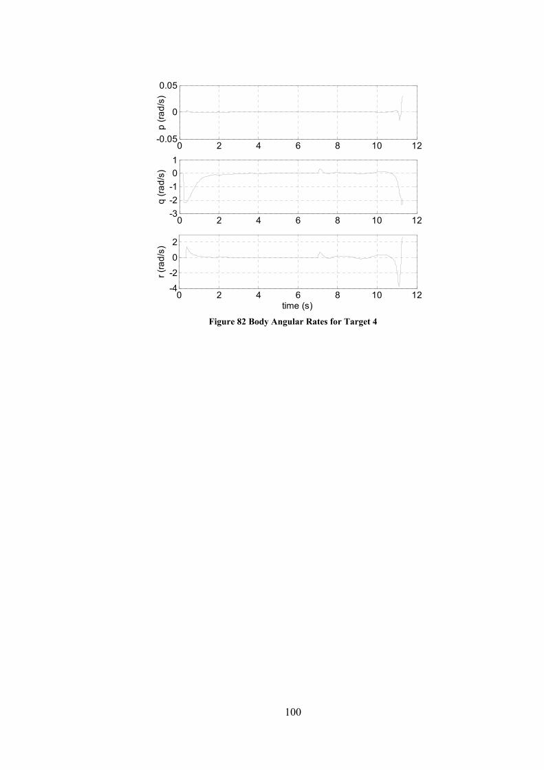
100

0 2 4 6 8 10 12-0.05

0

0.05

p (ra

d/s)

0 2 4 6 8 10 12-3-2-101

q (ra

d/s)

0 2 4 6 8 10 12-4

-2

0

2

time (s)

r (ra

d/s)


101

CHAPTER 7

TURNOVER STRATEGY ANALYSIS

In the previous section, in the vertical launch phase, the missile is controlled as it is

skid to turn. In this section, an enhanced strategy will be studied especially for the

turnover of the missile in short time. The proposed strategy is actually a mixed

ascend and turnover maneuver composed of an initial roll and then skid to turn.

That kind of maneuvering is also used for air to air missiles [3].

Figure 83 shows the expressed strategy. In vertical flight missile makes an initial

roll maneuver and then starts turn over maneuver. The main point of the initial roll

maneuver is that the pitch plane of the missile’s body coordinates is placed in

approximately the same vertical plane with the target. Hence, missile will need less

lateral acceleration and reduce sideslip angle. The results are discussed in details in

the following section.

102

Figure 83 Turnover Strategy

7.1. Initial Roll Maneuver Comparison of the Aerodynamic and Thrust Vector

Control

In this section, aerodynamic and thrust vector control over initial roll maneuver is

performed. A static target at [3000, 3000,-300] is being tried to hit with two

turnover strategy and with different control capabilities. The azimuth angle so the

initial roll command is 45°. In order to prevent wrong decision of autopilot because

of the Euler angles singularity at θ =90º, roll angle commands are generated with

integral of the roll rate. During the initial roll maneuver, yaw channel is not

controlled as it does not need control, the cross coupling terms do not result

effective yaw motion at velocities close to 0. But after initial roll, the yaw channel

and pitch channel control starts with respect to the guidance command profile.

Turnover Starting

Point

V

Skid to Turn

Initial Roll Maneuver

Vertical Flight

103

As shown in the previous chapters, during vertical flight missile velocity is very

low so the dynamic pressure, which means aerodynamic control, is insufficient and

this roll maneuver can be achieved in a short time with thrust vector control, but

the thrust vector control model described in section 3.4.2 cannot create axial

moment. But it is possible that if all of the jet vanes turn into the same direction for

the cruciform fin style and the resulting force can be multiplied with the distance

from the center of pressure of jet vane to the center of nozzle to create axial

moment (see Appendix). During the initial roll maneuver, all jet vanes are used for

roll maneuver and this necessity brings a modeling convenience for roll moment

created by thrust vector control system. As the nozzle and jet vane design is not the

subject of this thesis, from the fact defined above, an axial moment can been taken

into account linearly by aileron deflection. So, a look up table is implemented for

axial force moment for thrust vector control. The maximum value of axial moment

created with maximum jet vanes deflection is considered as 220 Nm which is a

realistic moment value. For example, [28] describes the moments and forces

created by jet vane thrust vector control system. In that study, large amount of lift

forces so the moments are created with a low level of thrust. Also, a simple thrust

vector control design is presented in the Appendix and the obtained maximum roll

moment is 217 Nm.

In order to examine effectiveness of the two different control inputs, initial roll

maneuver is commanded to place missile coordinates in approximately the same

vertical plane with the target. Roll command starts with simulation run time, after

0.3 seconds pitch and yaw channel autopilots are active. Figure 84 shows the roll

angle trend with two control technologies. As the roll moment created by TVC is

more than aerodynamic roll moment at the early times of vertical launch (<0.3s),

roll angle settles down quickly with TVC. Settling time of desired roll angle with

TVC is <0.3 seconds and <1.6 seconds with aerodynamic control.

104

0 1 2 3 4 5-50

-40

-30

-20

-10

0

time (s)

roll

angl

e ( °)

tvc rollaero roll

Figure 84 Roll Angle During Flight

Figure 85 and Figure 86 illustrate the trajectories, closing distance and velocity

profile with two control methods. They show that there is not a major difference in

the terms of flight time and closing distance. Angle of attack and sideslip profiles

are given in Figure 87. As seen, roll maneuver with TVC does not cause angle of

sideslip. Instead as missile is not at the same plane with the target with

aerodynamic roll maneuver in desired time interval, it has quite enough angle of

sideslip which is not different than skid to turn style.

105

Figure 85 Engagement Trajectory Comparison During Flight

0 2 4 6 80

1000

2000

3000

4000

RC

(m)

0 2 4 6 80

1

2

3

time (s)

VT (m

ach)

tvc rollaero roll

tvc rollaero roll

Figure 86 Closing Distance and Velocity Comparison During Flight

(Mac

h)

106

0 1 2 3 4 5 6 7 8-40

-30

-20

-10

0

10

β( °

)

0 1 2 3 4 5 6 7 8-80

-60

-40

-20

0

20

time (s)

α ( °

)

tvc rollaero roll

tvc rollaero roll

Figure 87 Angle of Sideslip and Attack Comparison During Flight

Figure 88 shows the body angular rates, as missile’s velocity and dynamic pressure

is not enough to create effective roll moment; the desired roll rate is developing

lately for aerodynamic roll control. However with TVC, the desired roll rate

develops quickly. Figure 89 shows the acceleration during flight. As the same

behavior, ay acceleration is used to turn towards the target, but there is very small

amount of acceleration in the Y axis (10-3) with initial roll control with TVC. As the

coordinates of the missile and target is in the same plane, missile just has az

acceleration to turnover to the target, which of all means, to have less lateral

acceleration and initial roll maneuver needs roll control with TVC.

107

0 2 4 6 8-6-4-20

p (ra

d/s)

0 2 4 6 8-6-4-20

q (ra

d/s)

0 2 4 6 80246

time (s)

r (ra

d/s)

tvc rollaero roll

tvc rollaero roll

tvc rollaero roll

Figure 88 Body Rates (p ,q, r) Comparison During Flight

0 2 4 6 8-400-200

0200400

a x (m/s

2 )

0 2 4 6 8-50

0

50

a y (m/s

2 )

0 2 4 6 8-50

0

50

100

time (s)

a z (m/s

2 )

tvc rollaero roll

tvc rollaero roll

tvc rollaero roll

“

Figure 89 Accelerations Comparison During Flight

108

7.2. Skid to Turn and Skid to Turn with Initial Roll Strategy Comparison

As explained in the previous chapter, if target and missile is going to be in the same

pitch plane, initial roll maneuver has to be performed quickly. After initial roll,

missile will turnover towards to the target rapidly. There is one point that has to be

considered, the results given in the previous sections are for static targets. A static

target which has a component in Y axis can be hit with only the initial roll and

pitch maneuver as seen. However, if target has a velocity with respect to the

missile, initial roll will not be enough to hit the target. So that, missile needs to use

its yaw channel autopilot as it is a skid to turn missile.

In order to analyze this maneuver, a target has been define at [5000,-2500,-500] m

and with velocity [100,100, 0] m/s. the same critics to switch to terminal phase is

used, FOV ± 3 degrees and lock on range is 3000 meters. If the simulations are

analyzed, flight time lasts for 12.75 seconds, and 5.83 seconds for midcourse

guidance phase. Desired roll angle and response of the system is given in Figure

90. Missile rolls and then it tries to hold that roll angle. Figure 91 shows

trajectories of missile and target with the two turnover strategies. As seen, there is

not much difference in the scope of trajectories. Figure 93 shows the closing

distance and the velocity profiles through flight time. As seen, there is not even a

major difference between two strategies, but there is a small different velocity trend

during turnover because thrust loss is not defined for roll channel deflection. Full

skid to turn strategy has much velocity loss during turn over than the suggested

turnover strategies. The final velocities are very close to each other, because initial

roll maneuver is performed where velocity is very low and the aerodynamic axial

force has not yet produced in large amounts.

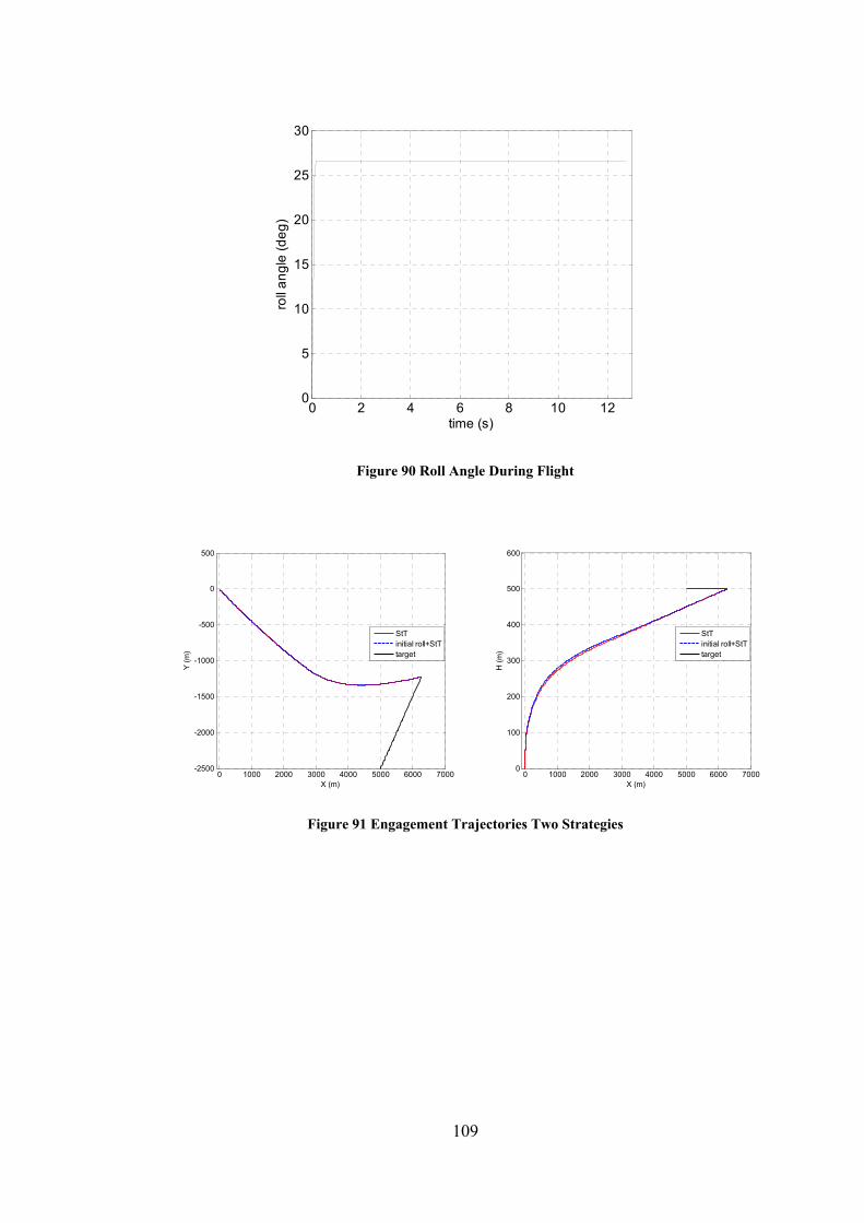
109

0 2 4 6 8 10 120

5

10

15

20

25

30

time (s)

roll

angl

e (d

eg)

Figure 90 Roll Angle During Flight

0 1000 2000 3000 4000 5000 6000 7000-2500

-2000

-1500

-1000

-500

0

500

X (m)

Y (m

)

StTinitial roll+StTtarget

0 1000 2000 3000 4000 5000 6000 70000

100

200

300

400

500

600

X (m)

H (m

)

StTinitial roll+StTtarget

Figure 91 Engagement Trajectories Two Strategies

110

0 2 4 6 8 10 120

1000

2000

3000

4000

5000

6000

time (s)

RC

(m)

StTinitial roll +StT

Figure 92 Closing Distance with Two Strategies

Figure 93 Velocity Profile with Two Strategies

Figure 94 is the angle of sideslip and attack during maneuvers. Skid to turn

strategy’s angle of side slip is approximately 25 degrees, but the suggested strategy

does not need to have a side slip angle because of the initial roll maneuver, and this

111

roll maneuver does not have a significant effect in the terminal phase tendency.

Angle of attack is approximately the same in the first phase (initial and midcourse),

but in the terminal phase, mixed strategy need a little much angle of attack than the

skid to turn. Maximum 4.6 degree of angle of attack for skid to turn and 1.6 degree

of angle of attack for the mixed strategy is obtained. However, this change can be

ignored with respect to the angle of sideslip difference.

0 2 4 6 8 10 12-20

0

20

40

β(°)

0 2 4 6 8 10 12-60

-40

-20

0

20

time (s)

α ( °

)

StTinitial roll+StT

StTinitial roll+StT

Figure 94 Angles of Sideslip and Attack with Two Strategies

Figure 95 explains one of the major differences between the two methods. In skid

to turn, missile has to reach a higher velocity value to have a body rate for yaw

maneuver; however in this strategy, missile rolls at a low velocity value and never

has a yaw rate in this scenario. After midcourse phase is over, missile has the same

trend in terminal phase. Figure 96 shows accelerations of missile during maneuver.

Axial accelerations are closely the same, but lateral accelerations differ as seen. It

is shown that skid to turn needs more lateral accelerations than the suggested

strategy, so the yaw rate. This initial roll strategy simplifies the maneuver and

reduces the required lateral accelerations, yaw or pitch plane, during the flight.

112

0 2 4 6 8 10 12-20246

p (ra

d/s)

0 2 4 6 8 10 12-6-4-202

q (ra

d/s)

0 2 4 6 8 10 12-6-4-202

time (s)

r (ra

d/s)

StTinitial roll+StT

StTinitial roll+StT

StTinitial roll+StT

Figure 95 Body Rates (p, q ,r) with Two Strategies

0 2 4 6 8 10 12-200

0

200

400

a x (m/s

2 )

0 2 4 6 8 10 12-100

0

100

200

a y (m/s

2 )

0 2 4 6 8 10 12-50

0

50

100

time (s)

a z (m/s

2 )

StTinitial roll+StT

StTinitial roll+StT

StTinital roll+StT

Figure 96 Accelerations with Two Strategies

113

CHAPTER 8

GUIDANCE DESIGN OPTIMIZATION

In this chapter, optimization via defined cost functions is applied to three chosen

problems of vertical launch missiles. After all, guidance commands are generated

as an output of the optimization. One of the main interests in this area is to analyze

and define the capability of the missile during rapid turnover for low altitude

targets. [60] is the only study found in literature on vertical launch missile turnover

optimization with a simple mathematical model. It uses differential dynamical

programming method and system is controlled with only thrust vector control.

In this thesis, the mentioned study is further enhanced and the optimization process

is applied over a 6 DoF nonlinear mathematical model. Thus, the first guidance

problem is based on the examination of the turnover capability of the missile.

Hence, the “Rapid Turnover Maneuver for Low Altitude Intercept” is studied and

the corresponding guidance commands are generated.

The second test case is cast in order to find a solution that gives an opinion on the

hybrid control ratio which drives the mechanical design and reduction ratio

between the thrust vector control and aerodynamic tail fins. The optimization is

mainly studied for “Intercept” maneuver that drives the missile to a constant

position within defense volume to intercept an attacking target.

The third test case is constructed to analyze the initial guidance phase which

actually results in a desired target intercept. Thus, the “Engagement Initiation”

114

maneuver is studied and the look angle of the missile is minimized to successfully

initiate the target intercept.

8.1. Real Coded Genetic Algorithm

Genetic algorithms, (GAs), are search methods based on the principles of natural

selection and genetics. They were first introduced by [61], and were extensively

explored by [62]. GAs have been proved to be efficient in many different areas

such as image processing [63], and system identification [64]. It is also possible to

see the application of genetic search methods in guidance and control, trajectory

optimization applications such as [65], [66] and [67]. Unlike the conventional

gradient based searching algorithms, GAs are inherently parallel, because they

simultaneously evaluate many points in the parameter space, called search space.

Real-coded genetic algorithm (RCGA) differs from the traditional binary-coded

GAs. It uses floating point representations in the searching procedure. The

chromosomes are the arrays of unknowns instead of bit strings. It works without

the need of coding and encoding procedures and reduces the computation time. The

procedure of real coded genetic algorithm applied in this study is given in Figure

97. Algorithm has fitness function, ordering, selection, crossover, mutation and

elitism algorithms for the best populations among the past and new populations.

115

Figure 97 Genetic Algorithm Search Procedure

Initialization: The initial population of candidate solutions is usually generated

randomly across the search space. However, domain specific knowledge or other

information can be easily incorporated. In this study, initial populations are

generated on basic knowledge of guidance commands generated from the

midcourse method mentioned in midcourse guidance section. Basic guidance

commands are then formed with random data production process. After then,

guidance commands are processed by a masking system which saturates the high

level guidance commands. Guidance commands are filtered with a low pass filter

in order to satisfy a guidance command frequency components at the end and the

time lag caused because of the filter is negligible.

116

Evaluation: Once the population is initialized or an offspring population is

created, the fitness values of the candidate solutions are evaluated.

Selection: Selection allocates more copies of those solutions with higher fitness

values and thus imposes the survival of the fittest mechanism on the candidate

solution. The main idea of the selection is to prefer better solutions to worse ones.

Roulette Wheel, stochastic universal, ranking and tournament selection are some of

the methods which are used generally. In this search algorithm, a linear function

mapping is used. The best and the worst fitness values are mapped to 0 and 1. The

other fitness functions so the populations are mapped in between them.

Crossover: Crossover combines parts of two or more parental solutions to create

new, possibly better solutions. The selected populations are chosen with Roulette

Wheel method). The number of crossover is predefined. Crossover procedure is

given in (8.1) where α is an algorithm parameter which is taken as 0.65 and s,p,s′

are vectors (chromosomes).

' . (1 ).s s pα α= + − (8.1)

Mutation: While crossover operates on parents, mutation locally but randomly

modifies a solution. Again there are many variations of mutations, but it is usually

involves one or more changes made to an individual’s traits. In addition to

classical mutation processes, the search algorithm increases both the search area

and the amplitude of mutation if the best fitness value is the same for last two or

more times of the generation.

Elitism: The method is also 1 elitist so the top performing individual of each

generation is assured to be included in the next population.

Replacement: The offspring population created by selection, crossover, mutation

and elitism replaces the original parental population. Many replacement techniques

117

such as elitist replacement, generation-wise replacement and steady state

replacement methods are used in genetic algorithms. Here, elitist replacement

method is used.

Decision Variables: In the construct optimization problem two decision variables

are considered. They are maximum generation number and fitness value. If the

maximum number of generation or the minimum fitness value is obtained, search

algorithm stops.

Cost Function to Fitness Function: There are several methods for calculation

fitness function over cost function. In this study, two methods are used. One of the

methods is normalizing the cost function and scaling it to a maximum and

minimum function values. Then minimum cost is converted maximum fitness and

vice versa. The second method is subtracting cost function from a very larger

number. As the cost function is minimized, result of the subtraction is increases.

8.2. Rapid Turnover Maneuver for Low Altitude Intercept

Rapid turnover maneuver requires high angle of attack capability. As seen in

Figure 98, missile launches vertically and starts to turn over at a safety altitude for

rapid turnover maneuver. At the end of the maneuver, missile velocity vector is

desired to be parallel to the inertial ( 0fγ = ) X axis which means missile can go

horizontally to the X axis. This maneuver usually defines missile critic

requirements. In order to analyze the designed missile turnover capability and

analyze the missile rapid turnover capability, an optimization algorithm is

implemented with real coded genetic search method.

118

Figure 98 Rapid Turnover Maneuver

Problem formulation can be defined as;

1- Minimize the rapid turnover altitude at minimum time with the constraints

that missile velocity vector is horizontal at this altitude

2- Minimize the rapid turnover maneuver time

So, the cost function is formulated as;

f1 2

f max max

minimize Jt hJ=

t hξ ξ+

(8.2)

where 1ξ and 2ξ are weighting coefficients. maxh and f maxt are the maximum

values of turning altitude and time. Results are normalized with respect to these

maximum values which are given in Table 12.

Turning Point

Vertical Flight

V

119

Table 12 Parameters for Rapid Turnover Maneuver Optimization

Variable Value

maxh 300 m

f maxt 3.5 s

1ξ 0.5

2ξ 0.5

Final condition of the simulation is 0fγ = that means velocity vector is parallel to

the X axis. The constraints in the optimization are:

20 20

350 350

90 90

0f

u

/ s q / s

α

γ

− ≤ ≤

− ≤ ≤

− ≤ ≤

=

(8.3)

Figure 99 and Figure 100 show the best fitness values and optimal guidance

command. Figure 101 illustrates the deflection command throughout the maneuver.

Figure 102 presents trajectories through generations. The maximum fitness value is

0.94 for the last 10 generations which lead us to at least a local optimal point. It

shows fitness values of improved populations. Elite population of the first

generation can only reach to altitude higher than 80 meters, however the 3rd, 6th and

14th generations elite populations can reach to 70 to 60 meters altitude with flight

path angle 0 degree. Through generations, the turnover range also decreases. The

range decreases from 250 meters to 50 meters.

120

0 5 10 15 20 25 300.76

0.78

0.8

0.82

0.84

0.86

0.88

0.9

0.92

0.94

number of generations

best

fitn

ess

Figure 99 Best Fitness Values for Elite Populations Through Generations

0 0.2 0.4 0.6 0.8 1

-60

-50

-40

-30

-20

-10

0

10

time (s)

guid

ance

com

man

d ( °)

Figure 100 Guidance Command

121

0 0.2 0.4 0.6 0.8 1

-5

0

5

10

15

20

time (s)

δ e( °)

Figure 101 Deflection Throughout the Maneuver

-50 0 50 100 150 200 2500

10

20

30

40

50

60

70

80

90

X (m)

H (m

)

g1g3g6g14g23

Figure 102 Trajectories for Elite Populations Through Generations

Figure 103 shows the velocity profile during rapid turnover maneuver. The first

elite population maneuver lasts for about 1.8 seconds and its last velocity is much

more than 1 Mach and the last generation’s elite population maneuver lasts for

about 1 second and finishes the maneuver less than 0.4 Mach. Also, the best elite

122

population linearly decreases flight path angle form 90 degrees to 0 degree in about

1 second, see Figure 104.

0 0.5 1 1.50

0.2

0.4

0.6

0.8

1

time (s)

VT (m

ach)

g1g3g6g14g23

Figure 103 Velocities for Elite Populations

0 0.5 1 1.50

10

20

30

40

50

60

70

80

90

100

time (s)

γ (°)

g1g3g6g14g23

Figure 104 Flight Path Angle for Elite Populations

(Mac

h)

123

8.3. Intercept Maneuver Analysis with Hybrid Control Ratio

As mentioned in the 3.4.2 the hybrid control ratio between aerodynamic control

and thrust vector control is a design decision. This ratio is the mechanical coupling

ratio of the control inputs, and it is not being changed during flight. For the sake of

simplicity, the hybrid control ratio had been decided according to the control

effectiveness of the two control inputs. As seen at Figure 21, the ratio of the control

inputs are close to each other after the velocity becomes higher than 1 Mach. To

have the same control effectiveness with aerodynamic control and use less thrust

vector control, the ratio had been taken 0.87. In order to analyze the chosen ratio’s

effectiveness and give an idea to hybrid control ratio decision, an optimization

process has been supplied. The optimization algorithm finds the optimal hybrid

control ratio K which couples both of the control inputs given at (8.4) and

optimizes its trajectory during the flight. Here, (8.4) is given to simplify the

problem and remind the term hybrid control ratio. However, the hybrid control

ratio is changed in the nonlinear simulation.

A 1 T 2

A T

x Ax B u B ux Ax ( B KB )u= + += + +

(8.4)

where A is system matrix, BA is the control input of aerodynamic control, BT is the

thrust vector control input matrices and the K is hybrid control ratio defined in

section 4.6.

In order to find an optimal hybrid control ratio, different points are defined. Missile

is trying to reach the desired points and optimization algorithm is trying to find a

feasible trajectory and hybrid control ratio. So, problem formulation of the

optimization can be given as;

Minimize maneuver time

Minimize miss distance

Minimize control effort which of all define the cost function below:

124

22

0

tf

f c

min imize J

J=t R ( u dt )+ + ∫ (8.5)

The constraints are;

20 20

350 350

90 90

u

/ s q / s

α

− ≤ ≤

− ≤ ≤

− ≤ ≤

(8.6)

As seen from the Table 13, hybrid control ratio increases whenever missile needs to

get close to a lower altitude. This result was an expected result, because missile

needs more acceleration to go a critical point such as 50 meters above ground

which means more control power requirement. Another result is the increase in the

final time of the maneuvers; on the contrary initial distance to the desired point is

decreasing. This result is also a result of a critical maneuver needs more time to be

successful. Miss distances are all less than 1 meter which is quite well. This result

remarks that an optimal trajectory is also found with real coded genetic algorithm

search method. Figure 105, Figure 106, Figure 107 and Figure 108 shows the best

trajectories and velocities of each point at each generation. Throughout generations,

miss distance is decreasing, but a generalization for final time cannot be made

directly, because at each flight the traveled distance is changing.

In conclusion, if a vertical launch missile control system will be a hybrid control,

the mechanical coupling ratio has to be considered with respect to the critical

maneuver. In this study, the ratio has been changed between 0.5 and 2.5. This

optimization study says that, the chosen ratio which was taken into account at the

early stages of the thesis is quite proper which defines the critical maneuver

between 100 and 300 meters altitude.

125

Table 13 Optimization Results for Trajectory and Hybrid Control Ratio

Desired Positions (m)

Miss Distance (m)

tfinal (s)

Hybrid Control Ratio

[1000;0;-50] 0.60 3.23 0.957

[1000;0;-100] 0.74 3.17 0.909

[1000;0;-300] 0.56 3.11 0.81

[1000;0;-500] 0.33 3.18 0.673

0 200 400 600 800 10000

50

100

150

200

250

X (m)

H (m

)

0 0.5 1 1.5 2 2.5 3 3.50

0.5

1

1.5

2

2.5

time (s)

VT (m

ach)

g1g4g12g18

g1g4g12g18

Figure 105 Trajectories and Velocities for Position 1

(Mac

h)

126

0 200 400 600 800 10000

50

100

150

200

X (m)H

(m)

0 0.5 1 1.5 2 2.5 30

0.5

1

1.5

2

time (s)

VT (m

ach)

g1g4g10g15

g1g4g10g15


0 200 400 600 800 10000

100

200

300

400

X (m)

H (m

)

0 0.5 1 1.5 2 2.5 30

0.5

1

1.5

2

time (s)

VT (m

ach)

g1g7g12g16

g1g7g12g16


(Mac

h)

(Mac

h)

127

0 200 400 600 800 10000

200

400

600

X (m)H

(m)

0 0.5 1 1.5 2 2.5 30

0.5

1

1.5

2

time (s)

VT (m

ach)

g1g8g11g16

g1g8g11g16


8.4. Engagement Initiation Maneuver Optimization

In the initial phase where missile is not yet pointed to the target, an initial guidance

can be defined that missile will be pointed to the target at the end of the initial

guidance that the maneuver in this phase is the engagement initiation maneuver.

After missile is pointed to the target, midcourse and terminal phase guidance

algorithms will be active. This pointing procedure is quite similar to trainable

launcher application, but here pointing missile to the target is a part of missile

guidance and control system not launcher’s mission and it is much more applicable

rather than trainable launcher. Launcher needs more space to turn 360º; however

missile can be pointed in any direction with its guidance and control system

without increased space need. There may be also other reasons for defining

engagement initiation maneuver; for example jet vanes may erode or thrust vector

control section is thrown away after turnover maneuver in order to inherit thrust

loss and extra weight of thrust vector control unit and because of these reasons,

initial guidance will be critical.

(Mac

h)

128

In the section, guidance of a vertical launch missile has been divided into three

phases; initial which is for engagement initiation, midcourse and terminal phases,

illustrated in Figure 109, and an optimization algorithm is applied in order to have

an optimal engagement initiation. In such an algorithm, elapsed time for maneuver

and successful pointing will be very critical. After engagement initiation, it is

important that missile can see or track the directed point and lock on the target.

Another critical parameter is the control effort, in other words energy optimization

has to be taken into consideration. To sum up, the cost function used for initial

guidance, the expressions are formulated in Eq. (8.7). Cost function is normalized

with maximum time, control effort and κ defined in Eq. (8.8). κ includes the

maximum term and also the square of look angle in order to have more effect. In

Eq. (8.7), 1ξ , 2ξ and 3ξ are weighting coefficients, ε is look angle, u is control

effort. maxft and maxfε are the maximum values of maneuver time and look angle.

NormalizeU is the maximum value for the energy cost. Results are normalized with

respect to these maximum values.

Figure 109 Guidance Strategy

129

2

01 2 3

tf

f

f max max Normalize

min imize J

u dtt

Jt U

κξ ξ ξκ

⎛ ⎞⎜ ⎟⎜ ⎟

= + + ⎜ ⎟⎜ ⎟⎜ ⎟⎝ ⎠

∫ (8.7)

[ ]

2

0 3 3k max

k

ε ε

κ ε

= − − −

= + (8.8)

Constraints of dynamical systems are obliquely the constraints of the optimization

algorithm which are given in Eq. (8.6).

Table 14 Parameters for Engagement Initiation Maneuver Optimization

Parameter Value f maxt 1.5 s

maxκ 12

NormalizeU 0.2

1ξ 0.4

2ξ 0.3

3ξ 0.3 Optimization results are summarized in Table 15. Some positions are defined and

some initial look angles related with the given positions are presented as example

look angles. Maximum fitness function, final time and velocity at the final time are

also shown in order to make comparison. Time to point the missile to a direction

that target is in the field of view, is decreasing as initial look angle is decreasing

and maximum velocity is decreasing as a consequence of this result. Look angles

progress for each example throughout generations are presented in Figure 110,

Figure 111 and Figure 112. Progress trend of each example differs, because of wide

range of initial condition of populations and mutation success. If Figure 112 is

analyzed carefully, initial guidance problem turns into initial guidance command

130

problem. For initial look angle less than 50 degrees, an optimal guidance command

for maximum 0.2 seconds is optimal initial guidance starting command.

Table 15 Optimization Results for Several Look Angles

Example Initial Look

Angle (º)

Position (m)

Max. Fitness

tfinal (s)

Velocity (Mach)

1st 83 [1000;0;-30] 4.94 0.525 0.329

2nd 73 [1000;0;-300] 4.94 0.522 0.33

3rd 63 [2000;0;-1000] 4.92 0.445 0.308

4th 53 [2000;0;-1500] 4.93 0.414 0.294

5th 26.6 [2000,0;-4000] 4.95 0.335 0.246

0 0.5 1 1.50

10

20

30

40

50

60

70

80

90

time (s)

look

ang

le ( °

)

g1g3g8g19

Figure 110 Look Angle Progress of the 1st Example

131

0 0.1 0.2 0.3 0.4 0.5 0.60

10

20

30

40

50

60

70

80

time (s)

look

ang

le ( °

)

g1g6g10g16

Figure 111 Look Angle Progress of the 2nd Example

0 0.2 0.4 0.6 0.80

10

20

30

40

50

60

70

time (s)

look

ang

le ( °

)

g1g3g7g14

Figure 112 Look Angle Progress of the 3rd Example

132

0 0.2 0.4 0.6 0.8 1 1.20

10

20

30

40

50

time (s)

look

ang

le ( °

)

g1g4g11g18

Figure 113 Look Angle Progress of the 4th Example

0 0.2 0.4 0.6 0.8 1 1.20

10

20

30

40

50

60

70

80

90

time (s)

look

ang

le ( °

)

g1g3g5g10

Figure 114 Look Angle Progress of the 5th Example

133

8.5. 3D Engagement with Sub-Optimal Initial Guidance

In this section the guidance commands obtained from optimizations, which are

calculated for the engagement initiation, are used within a 3D engagement scenario

considering the 6 DoF motion of the missile. In order to apply this test case, the

calculated optimal guidance commands, that steers the missile towards to the

targets defined in the previous section, are defined as a discrete function of look

angle. In order to calculate the command values with respect to the instantaneous

look angles a look up table is constructed using the results of the previous section.

Thus, the pre-determined optimal guidance commands are constructed to cover the

possible defense volume of the missile in a “sub-optimal” fashion.

Since the optimal guidance commands are already generated for pitch plane, if the

missile rolls initially to orient its body pitch plane motion to the same plane with

the target, this proposed that sub-optimal engagement initiation strategy can be

applied. After sub-optimal guidance phase with initial roll maneuver, midcourse

and terminal guidance algorithms, proposed in the Chapter 6, are applied with the

same switching criteria. Figure 115 shows the suggested guidance strategy. An

example scenario is applied for this guidance strategy. The target’s properties are

given in Table 16. This target has maneuver weaving maneuver in pitch and yaw

planes.

134

Figure 115 Guidance Strategy for 6 DOF Motion

Table 16 Target Properties for the Suggested Guidance Strategy

Initial Position (m)

[6000; -3000; -2500]

Initial Velocity (m/s) [ ]200 0 0−

Maneuver

Starts maneuvering at 2000 m closing distance the

with acceleration

ay=5.g.sin(0.1.π.t)

az=5.g.sin(0.1. π.t) Figure 116 presents the missile and target trajectory, as target has maneuver both in

pitch and yaw planes, and a constant velocity, all of the combinations of motion at

Vertical Flight

Roll Maneuver

Skid to Turn

Sub-Optimal Initial Guidance

Midcourse Guidance

Terminal Guidance

Skid to Turn Initial Roll

Skid to Turn

Turnover Starting

Point

135

each plane is given. Figure 117 shows velocity, angle of sideslip and attack. In the

midcourse phase missile has not a significant angle of side slip because of initial

roll maneuver. More than 20 degrees of angle of attack is seen in the optimal initial

guidance and midcourse guidance phases. Figure 118 illustrates the body rates of

the missile during flight. Although at the end of midcourse, body rates are quite

inconsiderable, as the guidance switches to terminal guidance body rates again

increase. Miss distance is 0.815 meters. Figure 119 illustrates the roll angle during

flight and Figure 120 shows the initial guidance command the look angle during

the initial guidance command.

0 1000 2000 3000 4000 5000

-4000

-2000

0

Y (m

)

X (m)

0 1000 2000 3000 4000 5000 60000

1000

2000

3000

Z (m

)

X (m)

-3000 -2500 -2000 -1500 -1000 -500 00

1000

2000

3000

Z (m

)

Y (m)

missiletarget

missiletarget

missiletarget

Figure 116 Missile Target Trajectory

136

0 2 4 6 80

1

2

3

V T(m

ach)

0 2 4 6 8-40

-20

0

20α

( °)

0 2 4 6 8-10

0

10

20

β ( °

)

time (s)

Figure 117 Velocity, Angle of Attack and Sideslip Angles

0 1 2 3 4 5 6 7 8 9

0

2

4

6

p(ra

d/s)

0 1 2 3 4 5 6 7 8 9-3

-2

-1

0

1

q (ra

d/s)

0 1 2 3 4 5 6 7 8 9-1

-0.5

0

0.5

r (ra

d/s)

time (s)

Figure 118 Body Rates of the Missile

(Mac

h)

137

0 2 4 6 80

5

10

15

20

25

time (s)

roll

angl

e ( °)

Figure 119 Roll Angle

0 0.2 0.4 0.6 0.8 10

20

40

60

look

ang

le ( °

)

0 0.2 0.4 0.6 0.8 1-80

-60

-40

-20

0

time (s)

initi

al g

uida

nce

com

man

d ( °)

Figure 120 Sub-Optimal Guidance Command and Look Angle

138

CHAPTER 9

DISCUSSION AND CONCLUSION

The aims of this study is to obtain a nonlinear model for a generic hybrid controlled

VLSAM, and analyze the constructed system under the effect of high angle of

attack flight characteristics by 6 DoF simulations and linearization.

The dynamic modeling of VLSAM is carried out by implementing the well-known

Newton-Euler equations with rigid body assumptions including thrust vector forces

and moments. This is followed by aerodynamic data construction. On the contrary

to the investigated literature, in which there is limited aerodynamic data with

limited numerical parameters due to confidentiality purposes, a new and complete

aerodynamic data base over a wide range of angle of attack values is generated.

This is generally done by using a semi-empirical aerodynamic data estimation tool,

Missile DATCOM. However, in order to complete the aerodynamic data set, the

generated set is tailored and extrapolated to α ≤ 90° flight regime. The general

tendencies of the aerodynamic coefficients with respect to different velocities are

presented and analyzed. Static stability and aerodynamic characteristics are

analyzed and results are discussed. After then, the accuracy and validity of the

constructed VLSAM model is investigated by 6 DoF nonlinear simulations.

In order to design autopilot a linearization algorithm is carried on. Since the system

under study has two different flight phases as the first phase where there is thrust

and the second phase without thrust, which are different from each other, the

linearization of the missile dynamics is separated in two different categories. Since

139

time is the most dominant parameter that affects the thrust, impulse, and, the mass,

inertia, center of gravity of the missile and the velocity variation of the missile in

that phase, the scheduling is done with respect to time for the boost phase.

Linearization scheduling is done with respect to velocity as it is done in the in the

conventional systems, for the second phase. After the linearization study, the

accuracy and validity of the linearized model are tested. This is done by comparing

the outputs of the linear system model with the outputs of the nonlinear system

model, under the effect of the control input commands, jet vanes and tail fins. The

nearly perfect match of the linear and nonlinear system outputs showed that the

scheduling with respect to time for the first phase and scheduling with respect to

velocity for the second phase of the flight can be used reliably for the linear system

models. Following the linearization of the nonlinear dynamics, with the proposed

scheduling methods, control sensitivity and stability analysis of the missile for the

vertical launch phase is carried out. This analysis showed that the kinetic energy of

the missile decreases with decreasing velocity. This causes the eigen values of the

linear system move to the right hand side of the imaginary axis.

Missile dynamics are separated into three planes, pitch, yaw and roll after

linearization. Controllers are designed as the missile is a skid-to-turn missile.

Controllers design is also challenging as the system parameters are changing

rapidly. Body rate, angle and acceleration autopilots are designed with classical

approaches. The reasons behind the different autopilot types are to examine

different dynamic behaviors and to be adaptable to guidance requirements. As

autopilot design phase is considered before the design of guidance algorithms,

autopilot has to respond the guidance command and/or conversion logic has to be

designed. Autopilot performances are tested in the nonlinear model. According to

the outputs, designed autopilots have different performance characteristics. Angle

autopilot has the best performance than rate autopilots. This autopilot is

compensating the fast dynamics in the inner loop, and the outer loop compensates

the relatively slow dynamics. Moreover, the other autopilot types can also be used

with proper guidance algorithms.

140

Next, body pursuit guidance as midcourse guidance and proportional navigation

guidance for terminal guidance are studied and implemented. Switching conditions

from midcourse to terminal are determined. For yaw and pitch planes, angle

autopilots are chosen for the midcourse guidance phase and acceleration autopilot

is used for the terminal phase. In the roll plane body rate autopilot is preferred for

all of the flight time. After guidance algorithms are implemented, target sets are

defined and categorized into two sets as non maneuverable and maneuverable. The

first target set includes a low altitude static target and a target which is crossing and

diving with constant velocities is chosen. The second target set consists of

maneuverable targets, one is an oncoming target and the other is a target that has a

weaving maneuver in the terminal phase. The nonlinear simulations with the

designed autopilots and guidance algorithms have successful results on the target

sets. Some critical parameters such as angle of attack and side slip, body rates,

accelerations and trajectories are also presented.

In addition to guidance and autopilot algorithm development, a different turnover

strategy is suggested. Here, missile has an initial roll maneuver in order to be in the

same vertical plane with the target during vertical launch and so, missile has less

acceleration in yaw plane and has significantly less angle of side slip. The

comparison of initial roll maneuver with thrust vector control or aerodynamic

control is also examined. Differences of the roll maneuver with aerodynamic and

thrust vector control surfaces are shown and conclusions are presented, then. As it

is not possible to control the missile with aerodynamic control surfaces when the

missile velocity is close to 0, initial roll maneuver with aerodynamic control causes

nothing but very close skid-to-turn mode and missile has angle of sideslip because

of that. However, initial roll maneuver with thrust vector control does not have any

angle of sideslip for the same target. This result was an expected results and the

importance of thrust vector control in the initial phase of the missile is thus

exhibited.

The last part of the thesis includes some critical maneuver optimizations. All of the

optimization algorithms produce guidance commands. Open loop guidance

141

commands are performed by autopilots. In this section, a rapid turnover maneuver

optimization is carried on firstly. The aim of this is to optimize the most critical

maneuver for a very low altitude target. The second optimization problem is

studied for suggesting a methodology to define the hybrid control ratio which is a

mechanical coupling and has a preset value. In this methodology, some critical

positions are chosen and the missile is guided to these points optimally. Miss

distance and hybrid control ratios are presented. In this search, it is obtained that

for a critical maneuver missile needs more control power as expected. So, it can be

clearly said that hybrid ratio can be pre-set with respect to the desired tactical

requirements. Lastly, engagement initiation maneuver optimization is studied and

initial guidance commands are generated. The first aim of this optimization is to

search for the optimal guidance commands to direct the missile to the target. The

second aim is to define criteria for thrust vector usage. As it is well known, in some

applications jet vanes are not in use for the whole flight time. As the jet vanes are

the cause of extra drag, they result in some decrease in velocity. Thrust vector

control unit may be preferred to be erodable or they may be jettisoned during flight.

The problem is to determine the maximum duration that the jet vanes have to be

effective. Here, the guidance commands are found which yields answers to the

problems above implicitly. In order to merge the open and closed loop guidance,

the optimal open loop guidance commands are generated for some initial look

angles and interpolated. The different turnover strategy and the open loop guidance

command set is implemented for the nonlinear simulation. Open loop guidance

commands are scheduled with respect to the look angle. This strategy is performed

with a maneuvering target. A miss distance less than 1 meter is obtained.

We think that the present study needs some improvements in the following issues:

1. Intercept maneuvers can be enlarged to cover all the space with a varying

hybrid control ratio (two actuators for two control surfaces as in some

applications) and it can be developed for intercept positioning instead of

body pursuit midcourse guidance.

2. Full range guidance algorithms can be developed by merging the initial

TVC regime with the aerodynamic tracking guidance regime.

142

3. Developed controllers / autopilots can be improved by using more advanced

controller design techniques such as adaptive control.

4. Controllers are going to be developed which utilizes all the control surfaces

at the same time.

We plan to continue our academic work in these topics and a set of publications

will be prepared.

143

REFERENCES

[1] M.J. Hemsch, “Tactical Missile Aerodynamics: General Topics”, Vol. 141,

Progress in Astronautics and Aeronautics, AIAA, Washington DC. 1992.

[2] P. Zarchan, “Tactical and Strategic Missile Guidance”, Vol. 124, Progress in

Astronautics and Aeronautics, AIAA, Washington DC. 1990.

[3] K. A. Wise, D. J. Broy, “Agile Missile Dynamics and Control”, Journal of

Guidance, Control and Dynamics, Vol. 21, No. 3, June 1996.

[4] A. Thukral, M. Innocenti, “A Sliding Mode Missile Pitch Autopilot Synthesis

for High Angle of Attack Maneuvering”, J. Propulsion, Vol. 6, No. 3, May 1998.

[5] A. Facciano, K. Seybold , T. Kutz ,D. Widmer, “Evolved Seasparrow Missile

Jet Vane Control System Prototype Hardware Development”, J. Spacecraft and

Rockets, Vol. 39, No. 4, pp. 522-531, 2002.

[6] R. Solis, “An Analysis of the Vertical Launch Phase of a Missile Concept”,

AIAA, Aerospace Sciences Meetings, January 1983.

[7] C.Y. Kaya, “Thrust Vector Control of a Rocket Vehicle Associated with

Aerodynamic Control”, M. S. Thesis Mechanical Eng., METU, October 1989.

[8] E. Erdem, “Thrust Vector Control with Secondary Injection”, M. S. Thesis

Mechanical Eng., METU, September 2006.

[9] Ö. Atesoglu, “High Alpha Maneuvering and Stabilization Control of Flight

Vehicles”, Phd. Thesis Mechanical Eng., METU, July, 2007

[10] http://en.wikipedia.org/wiki/Vertical_launching_system_20_05_2010.

[11]http://defense-studies.blogspot.com/2010/07/hmasnewcastle-and-hmas

warramunga.html

[12] http://en.wikipedia.org/wiki/File:Buk-M1-2_9A310M1-2.jpg.

[13] www.en.wikipedia.org/wiki/IRIS-T, 12 January 2010.

[14]http://www.deneldynamics.co.za/brochures/Broc0266_Umkhonto-

IR%20external.pdf.

[15] www.en.wikipedia.org/wiki/MBDA_MICA, 14 January 2010.

144

[16] http://en.wikipedia.org/wiki/LFK_NG, 14 October 2009.

[17] www.en.wikipedia.org/wiki/Umkhonto, 1 February 2009.

[18] Control Actuation System Workshop/System Analysis Reference, Martin

Marietta Training Notes, Martin Marietta Inc., 1993.

[19] R.F.H. Woodberry, R.J. Zeamer, “Solid Rocket Thrust Vector Control”,

NASA-SP-8114, 1974.

[20] http://www.armscontrolwonk.com/images/1472.jpg.

[21]http://www.knovel.com/web/portal/browse/Thrust_Vector_Control.

[22] P. H. Reisenthel, “Development of a Nonlinear Indicial Model for

Maneuvering Fighter Aircraft”, AIAA Aerospace Sciences Meeting, 1996.

[23] M. Y Park, W. Kim, S. Kim, S. H. Park and J. W. Lee, “Asymmetric Vortices

Around a Body in a High Angle of Attack Supersonic Flow” Journal of the Korean

Physical Society, Vol. 55, No. 5, November 2009.

[24] H. Sadeghi, M. Mani, M. A. Ardakan, “Effect of Amplitude and Mean Angle

of Attack on Wake of an Oscillating Airfoil”, World Academy of Science,

Engineering and Technology, 2008.

[25] E. Abney, M. McDaniel, “High Angle of Attack Aerodynamic Predictions

Using Missile Datcom”, AIAA Applied Aerodynamics Conference, June 2005.

[26] Ö. Ateşoğlu, “Different Autopilot Designs and Their Performance Comparison

for Guided Missiles”, M .S. Thesis Aerospace Eng., METU, December 1996.

[27] P.K. Menon, E. J Ohlmeyer,” Integrated Design of an Agile Missile Guidance

and Control Systems”, Proceedings of the 7th Mediterranean Conference on Control

and Automation (MED’99), June 1999.

[28] E. Orbekk, “Thrust Vector Model and Solid Rocket Motor Firing

Validations”, 44th AIAA/ASME/SAE/ASEE Joint Propulsion Conference and

Exhibit, July 2008.

[29] A. I. El-Sharkawy, “Experimental Studies on Thrust Vector Control in Solid

Propellant Rockets”, 13rd AIAA/SAE Propulsion Conference, July 1977.

[30] G. Sung, Y. S. Hwang, “Thrust-Vector Characteristics of Jet Vanes Arranged

in X-Formation within a Shroud”, Journal of Propulsion and Power, Vol. 20, No. 3,

2004.

145

[31] E. Orbekk, “Novel TVC System Utilizing Guide Vanes With Jet Flap’s İnto A

High Efficiency Compact Nozzle”, 41st AIAA/ASME/SAE/ASEE Joint Propulsion

Conference and Exhibit, July 2005.

[32] P.A Giragosian, “Theoretical and Experimental Aerodynamic Correlation of

Jet Vane Control Effectiveness, AIAA Atmospheric Flight Mechanics Conference,

August 1981.

[33] V. Harrisson, A. deChamplin, D. Kretschmer, R. Farinaccio, R. A. Stowe,

“Force Measurement Evaluating Erosion Effects on Jet Vanes for a Thrust Vector

Control System ”, 39th AIAA/ASME/SAE/ASEE Joint Propulsion Conference and

Exhibit, July 2003.

[34] R. Tekin, Ö. Atesoğlu, K. Leblebicioğlu, “Modeling and Vertical Launch

Analysis of an Aero- and Thrust Vectored Surface to Air Missile”, AIAA

GNC/AFM/MST/ASC/ASE Conference, August 2010.

[35] http://www.scribd.com/doc/12515933/Tactical-Missile-Design-

Presentation-Fleeman, 02_17_2009.

[36] L. H. Smith, R. H. Nunn, “Aerodynamic Characteristics of an Axisymmetric

Body Undergoing a Uniform Pitch Motion”, J. Spacecraft, Vol. 13, No. 1, January

1976.

[37] J. E. Fidler, M. C. Bateman, “Asymmetric Vortex Effects on Missile

Configurations”, J. Spacecraft, Vol. 2, No. 11, November 1975.

[38] A. B. Wardlaw Jr., A.M. Morrison, “Induced Side Forces on Bodies of

Revolution at High Angle of Attack”, J. Propulsion, Vol. 3 No. 10, October 1976.

[39] H. Jorgensen, “Reduction of Static Aerodynamic Characteristics for Slender

Bodies with Lifting Surfaces at very High Angle of Attack”, NASA TR R-474,

September 1977.

[40] J. Nielsen, “The Present Status and the Future of Missile Aerodynamics”,

NASA N88-29773, January 1988.

[41] Martin Marietta, “Aerodynamic Stability Technology for Maneuverable

Missiles”, AFFDL-TR-76-55 Vol. 1, March 1979.

[42] P. Giragosian, “Aerodynamic Considerations in the Design of a Vertically

Launched, Advanced Interdiction Missile”, AIAA Atmospheric Flight Mechanics

Conference, August 1982.

146

[43] D. E Lesieutre, J. Love, M. Dillenius, “High Angle of Attack Missile

Aerodynamics Including Rotational Rates-Program M3HAX”, Atmospheric Flight

Mechanics Conference, July 1996.

[44] P. Liu, X. Deng, “Experimental Investigation of Aerodynamic Characteristics

on Slender Bodies at High Angle of Attack”, Vol. 49, No. 1, March 2003.

[45] E. Smith, S. Hebbar, M. Platzer, “Aerodynamic Characteristics of a Canard

Controlled Missile at High Angle of Attack”, Journal of Spacecraft and Rockets,

Vol. 31, No. 5, October 1994.

[46] R. Tekin, Ö. Ateşoğlu, K. Leblebicioğlu, “Bir Hava Savunma Füzesinin Dikey

Fırlatma Fazının ve Etkin Dönme Manevralarının İncelenmesi”, 5. Savunma

Teknolojileri Kongresi, June, 2010.

[47] S. Wassom, L. Faupell,” Integrated Aerofin/Thrust Vector Control for Tactical

Missiles”, J. Propulsion, Vol. 7, No. 3, June, 1991.

[48] E. Devaud, H. Siguerdidyane, S. Font, “Some Control Strategies for a High

Angle of Attack Missile Autopilot”, Control Engineering Practice 8, pp. 885-892,

2003.

[49] H. Buschek, M. McDaniel, “Design and Flight Test of a Robust Autopilot for

IRIS-T Air to Air Missile”, Control Engineering Practice 11, pp. 551-558, 2003.

[50] H. Buschek, “Full Envelope Autopilot Design Using Gain Scheduled Robust

Control”, Journal of Guidance, Control and Dynamics, Vol. 22, No. 1, pp. 115-122,

1999.

[51] R. Tekin, Ö. Ateşoğlu, K. Leblebicioğlu, “Hibrit Kontrollü - Dikey Fırlatılan

Bir Hava Savunma Füzesinin Dinamiği ve Hızlı Dönüş Manevrası için Otopilot

Tasarımı”, Otomatik Kontrol Ulusal Toplantısı, September 2010.

[52] C. Song, “Adaptive Control of Linear Time Varying Systems with

Applications to Missile Autopilots”, Phd. Thesis, University of Florida, 1989.

[53] A. Tsourdos, B. A. White, Adaptive Flight Control Design for Nonlinear

Missile”, Control Engineering Practice,Vol. 13, No. 3, pp.373-382, 2005.

[54] T. B. Mull, “Use of Minimum Time Controllers in Vertically Launched

Surface to Air Missiles “, Master Thesis, Naval Postgraduate School, June 1992.

[55] K. S. Erer, R. Tekin, “İleri Hız Değişiminin Füze Yanal Dinamiğine Etkileri

Üzerine Bir İnceleme“, Otomatik Kontrol Ulusal Toplantısı, September 2010.

147

[56] K. Ogata, “Modern Control Engineering”, Prentice Hall, 4th Edition, 2002.

[57] A. Arrow, D. E. Williams, “Comparison of Classical and Modern Missile Autopilot Design and Analysis Techniques”, J. Guidance, Vol. 12, No.2, pp. 220-227, 1987. [58] R. Tekin, Ö. Ateşoğlu, K. Leblebicioğlu, “ Çevik Füze Dinamiği ve Denetimi

Üzerine Temel İncelemeler”, Ulusal Havacılık ve Uzay Konferansı, September

2010.

[59] http://acgsc.org/Meetings/Meeting_97/General%20Session/4.2.2.1.ppt.

[60] H.O. Jonnson, G. Malmberg, “Optimal Thrust Vector for Vertical Launch of

Tactical Missiles”, Journal of Guidance, Control, and Dynamics, Vol. 5 No. 1, pp:

17-21, 1982.

[61] J.H. Holland, “Adaptation in Natural and Artificial Systems“, University of

Michigan Press, Ann Arbor, MI, 1975.

[62] D.E Goldberg, “Genetic Algorithm in Search, Optimization, and Machine

Learning”, Addison-Wesley, Reading, MA, 1989.

[63] D.M. Etter, M.J. Hicks, K.H. Cho, “Image Registration by Genetic Search”

Proc. IEEE Soueastcon’84, pp. 460–464, 1984.

[64] K. Kristinsson, D.A Dumont, “Genetic Algorithms in System Identification”,

3rd IEEE Int. Symp. Intell. Contr., Arlington, VA, pp. 597–602, 1988.

[65] L.S Crawford, V.H.L Cheng, P.K. Menon, “Synthesis of Flight Vehicle

Guidance and Control Laws Using Genetic Search Methods”, AIAA Guidance and

Navigation Conference, August 1999.

[66] C.L. Lin, R-M. Lai, “Parameter Design for a Guidance and Control System

Using Genetic Approach”, Aerospace Science Technology 5, pp: 425–434, 2001.

[67] A. H. Kasem, “Trajectory Optimization via Simulation Using Incremented

Genetic Algorithms”, the Canadian Aeronautics and Space Journal, Vol. 52, No. 1,

March 2006.

148

APPENDIX

THRUST VECTOR CONTROL MODELING

Jet vanes are fins mounted at the exit of a rocket nozzle, Figure 121. The purpose is

to deflect part of the flow, thus providing side force. In order to give an idea of the

lift force created by a jet vane, a simplified analytical model is presented.

Figure 121 Jet Vane

The simplified model is for jet vanes that are not in a shroud but at the end of the

nozzle exit and the position of the jet vanes are important. The lift force produced

by jet vanes corresponds to the side force that jet vane system generates. 2D

analysis overestimates the lift force generated by a real jet vane. This is caused by

wing effects in the supersonic flow. In some references, a constant value is

149

suggested as a correction factor. In many cases, linear theory is enhanced with

experiments and a correction factor is determined for the specific case. However, in

order to give a brief idea about thrust vector modeling, these assumptions are not

taken into account and basic thrust vector modeling is expressed.

To determine the lift force calculations from linear theory, the following equations

can be directly applied. The lift and drag forces on a jet vane is

21

2 LL PC M Sγ ∞=

21

2 DD PC M Sγ ∞=

where

• P : Pressure

• M∞ :Velocity at the exit of the nozzle

• S : Reference surface

• γ : Specific heat ratio

• LC and DC : Lift and drag coefficients of the jet vane

• L : Lift

• D : Drag

and

.S c s=

where s is span and c is chord of the jet vane. It is also possible to define S, the reference surface as function of time as there is

erosion on the surface of the vane with respect to the vane material and motor

output materials.

The lift and drag coefficients are

150

2

41

LCMδ

∞

=−

2

2

2

41

kD

tCcM

δ∞

⎛ ⎞⎛ ⎞= +⎜ ⎟⎜ ⎟⎜ ⎟⎝ ⎠− ⎝ ⎠

where

δ is deflection of the jet vane, c is chord and tk is thickness.

Forces generated on the vane opposite of the flow are the cause of the drag force.

Total drag force is the sum of the each drag force of each jet vane and it can be

expressed as below:

1 2 3 4loss drag drag drag dragT F F F F= + + +

Figure 122 “+” Form Jet Vane Configuration

Thrust forces and moment equations for “+” form jet vane configuration illustrated

in Figure 122 is given below:

151

1 3

4 2

Tx loss

Ty Lift LiftT

z Lift Lift

F T TF F FF F F

⎡ ⎤ ⎡ ⎤−⎢ ⎥ ⎢ ⎥= −⎢ ⎥ ⎢ ⎥⎢ ⎥ ⎢ ⎥−⎣ ⎦⎣ ⎦

1 2 3 4( )...

TLift Lift Lift Lift t

T Ty y TT T

z z T

L F F F F lM F lM F l

⎡ ⎤ + + +⎡ ⎤⎢ ⎥ ⎢ ⎥=⎢ ⎥ ⎢ ⎥⎢ ⎥ ⎢ ⎥⎣ ⎦⎣ ⎦

where T is the main thrust. In this equation, the moments created by drag forces

are neglected.

Moment arm in the equation of roll moment created by thrust vector control system

is tl and it is the distance from nozzle center to the center of pressure on the jet

vane. The moment arm of roll moment can be expressed as;

2tl d coP= −

where d is the nozzle exit diameter and coP is the center of pressure.

The moment arm for pitch and yaw moments is, Tl , the distance between center of

gravity of the missile and center of gravity of thrust vector control system which is:

_T cg cg tvcl x x= −

Total side force is defined as:

2 2

side y zT F F= +

Total thrust deflection angle is

θ =arctan ( )side

loss

TT T−

.

152

Table 17 shows the parameters for a simple jet vane system design for the thesis.

Table 17 Motor and Jet Vane Parameters

Thrust 35000 N

Pressure 368417 Pa

Mach 2.9

Chord, c 0.084 m

Span, s 0.041m

Gamma,γ 1.17

Thickness, kt 0.009

Roll moment arm, tl 0.018 m

Table 18 shows the lift and drag forces of one jet vane at 10 and 20 degrees of

deflection. 3012 N lift force and 362 N drag force is obtained at 20 degrees of

deflection. It is obvious that lift force is a linear function of jet vane deflection but

not the drag force.

Figure 123 shows the lift and drag force trend from 0 to 20 degrees of jet vane

deflection.

Table 18 Lift and Drag Force Results from Linear Theories

Deflection (°) Lift(N) Drag(N)

10 1506 362

20 3012 1150

153

0 5 10 15 200

500

1000

1500

2000

2500

3000

vane deflection (°)

(N)

Figure 123 Lift and Drag Force of the Jet Vane

Critic design specifications of this system are given in Table 18. In this system at

least, maximum %13.15 of the main thrust is lost because of drag forces.

Maximum side force is 8520 N. Maximum roll moment is 217 Nm when if all the

jet vanes are deflected for roll motion. Maximum azimuth and elevation angles are

11.21 degrees. The relation between azimuth or elevation deflection and jet vane

deflection is 0.56T tvcθ δ= . These results are outputs of the linear theory; as it is

well known these results are overestimated values. However, a better motor and jet

vane can be designed. But this is out of the aim of this thesis.

Table 19 Critical Results from Linear Theories

Thrust Loss %13.15

Max. Side Force 8520 N

Max. Roll Moment 217 Nm

Azimuth, Tθ 11.21°

Elevation, Tψ 11.21°

DESIGN, MODELING, GUIDANCE AND CONTROL OF A VERTICAL

Documents

Transcript of DESIGN, MODELING, GUIDANCE AND CONTROL OF A VERTICAL