Design and Modeling of Real-time Shared-Taxi Dispatch Algorithms

1

Jung, Jayakrishnan, and Park

Design and Modeling of Real-time Shared-Taxi Dispatch Algorithms 1

2

Jaeyoung Jung* 3

Assistant Research Scientist, Ph. D. 4

Institute of Transportation Studies 5

University of California, Irvine 6

4000 Anteater Instruction and Research Bldg (AIRB) 7

Irvine, CA 92697-3600 8

Phone: +1–949–824–5989 / FAX: +1–949–824–8385 9

Email: [email protected] 10

11

12

R. Jayakrishnan 13

Professor 14

Institute of Transportation Studies 15

Department of Civil and Environmental Engineering 16

University of California, Irvine 17

4000 Anteater Instruction and Research Bldg (AIRB) 18

Irvine, CA 92697-3600 19

Phone: +1–949–824–2172 / FAX: +1–949–824–8385 20


22

23

Ji Young Park 24

Associate Research Fellow, Ph. D. 25

Office for Convergence Technology 26

The Korea Transport Institute 27

315, Goyangdaero Ilsanseo-gu 28

Goyang-si, Gyeonggi-do 411-701, South Korea 29

Phone: +82-31-910-3163 / FAX: +82-31-910-3227 30


32

33

34

35

36

37

38

39

40

41

42

43

44

45

*Corresponding author 46

Submission data: August 1, 2012 47

Paper length: 5850 + 250*8 (figures and tables) = 7850 words 48

49

TRB 2013 Annual Meeting Paper revised from original submittal.

2


ABSTRACT 1

Taxi is certainly the most popular type of on-demand transportation service in urban areas because taxi 2

dispatching systems offer more and better services in terms of shorter wait times and travel convenience. 3

However, a shortage of taxicabs has always been critical in many urban contexts especially during peak 4

hours and taxi has great potential to maximize its efficiency by employing shared-ride concept. There are 5

recent successes in real-time ridesharing projects that are expected to bring substantial benefits on energy 6

consumption and operation efficiency, and thus it is essential to develop advanced vehicle dispatch 7

algorithms to maximize occupancy and minimize travel times in real-time. This paper investigates how 8

taxi services can be improved by proposing shared-taxi algorithms and what type of objective functions 9

and constraints could be employed to prevent excessive passenger detours. Hybrid Simulated Annealing 10

(HSA) is applied to dynamically assign passenger requests efficiently and a series of simulations are 11

conducted with two different taxi operation strategies. The simulation results reveal that allowing ride-12

sharing for taxicabs increases productivity over the various demand levels and HSA can be considered as 13

a suitable solution to maximize the system efficiency of real-time ride sharing. 14

15

16

17

18

19


3


Design and Modeling of Real-time Shared-Taxi Dispatch Algorithms 1

1. INTRODUCTION 2

Real-time ridesharing is defined as dynamically utilizing the empty seats in passenger cars by assigning 3

passengers on demand, which is quite different from the early version of carpooling projects that were not 4

feasible for real-time response due to the lack of advanced information technologies. As real-time 5

ridesharing projects have been successfully initiated, the potential benefits of ridesharing are expected to 6

be substantial in reducing fuel consumption, carbon emissions, and traffic congestion. For customers, 7

ridesharing can also reduce travel costs for driving and parking. Newer design of Demand Responsive 8

Transit (DRT) with true real-time routing, which can be named RTRT (Real-Time Routed Transit 9

Systems) have emerged in recent years (1, 2, and 3), but those concepts are not fully refined for practical 10

service in real world. Zimride, Avego, and SideCar (4, 5, and 6) are well known services recently initiated 11

for private ridesharing by simply matching drivers and riders in real-time as passengers travel in urban 12

areas. These services utilize vehicles operated by regular car owners and not commercial drivers. 13

However, it has been known that those private ridesharing services could raise potential concerns 14

about passenger insurance and fare-collection system since the service vehicles are operated by private 15

vehicles and drivers. In addition, rideshare on any given vehicle can be offered only when that private 16

vehicle is moving, and not all the time. To overcome these issues, real-time shared-taxi offers an 17

alternative that is similar. Shared-taxi can be characterized as an on-demand ride-share service operated 18

by an online dispatch center such that the system is capable of taking service requests from individual 19

customers in real-time and establishing service vehicle schedules. While real-time dispatching of such 20

systems is a new concept, shared-ride in taxi, at least in certain forms, is not new. According to a study by 21

Cervero (7), it already flourished in Washington D.C. during World War II due to gas shortage. Taxicab 22

drivers displayed their current destination signs so that riders would hail the cabs to share the ride to the 23

same destinations. For an example of an online real-time response taxi service, Uber (8) in certain U.S. 24

urban areas provides a Smartphone-based on-demand taxi service, though not involving ridesharing yet 25

because taxi-sharing is currently prohibited by law in many cities in the U.S. However, shared-taxi 26

services are being initiated in many countries. In China, the Beijing government recently allowed taxi-27

sharing due to the shortage of taxicabs during rush hours. That scheme however required all passengers to 28

get in the car at the same location. In Singapore, Taiwan, and Japan, dynamic shared-taxi services are 29

conducted or initiated to link passengers who travel to the same area (9, 10, and 11). 30

In this paper, an optimization scheme is developed for the real-time vehicle routing in fully 31

flexible shared-taxi systems and a simulation study is conducted to investigate how such a shared-taxi 32

system can improve passenger travel compared to conventional taxi services by utilizing vehicle 33

resources more efficiently. Real-time shared-taxi operation with associated algorithms is studied with 34

realistic scenarios, to evaluate the system performance and the efficiency of solving the vehicle routing 35

problem. The remainder of the paper is organized as follows. In the next section, the real-time shared-taxi 36

is specified as a constrained problem of pickup and delivery for dynamic ride-sharing and three different 37

algorithms are provided. Next, a simulation environment is introduced with two different taxi operation 38

schemes. Finally, the simulation results are discussed with a sensitivity analysis. 39

2. REAL-TIME SHARED-TAXI DISPATCH PROBLEM 40

In many countries, taxis are operated by an online dispatch center with the help of communication 41

technologies and geo-location services by utilizing GPS (Global Positioning System) and digital maps. 42

Since providing a quality passenger service requires fast and efficient vehicle dispatch algorithms, it is 43

assumed that online taxi dispatch systems are operated with the help of computer algorithms, advanced 44

communication, and Automatic Vehicle Location (AVL) systems. Cervero (7) differentiates such services 45

from conventional carpooling services in several ways: (1) Vehicles are operated by taxi drivers; (2) 46

Vehicle pickup schedules are assigned dynamically to minimize passenger waiting time and in-vehicle 47

travel time; (3) Vehicle operations are scheduled and controlled by the central dispatch system. The use of 48


4


shared-ride concept in taxi service allows passengers to satisfy the riding public’s preference as well as to 1

save costs. 2

In real-time taxi dispatch system, when a new request is identified by the system operator, the 3

service request is delivered to the system queue where each customer is labeled with time windows and 4

locations of trip origin and destination. Meanwhile, the dispatch algorithm takes a service request from 5

the queue and finds a best available taxi for the travel request within the time windows. If there’s no 6

available taxi to meet the constraints, the dispatch system can reject the request. Once a vehicle is 7

assigned the updated schedule, the vehicle uses the shortest (fastest) path to the pickup and drop-off 8

locations based on real-time traffic information provided by the dispatch system. 9

In a shared-taxi system, the dispatch algorithm needs to find not only the best available vehicle 10

among candidates, but also an optimal route with the newly updated schedules that avoids the violation of 11

vehicle capacity constraints and the time window constraints of previously assigned passengers as well as 12

the new passenger. 13

14

15 (a) (b) 16

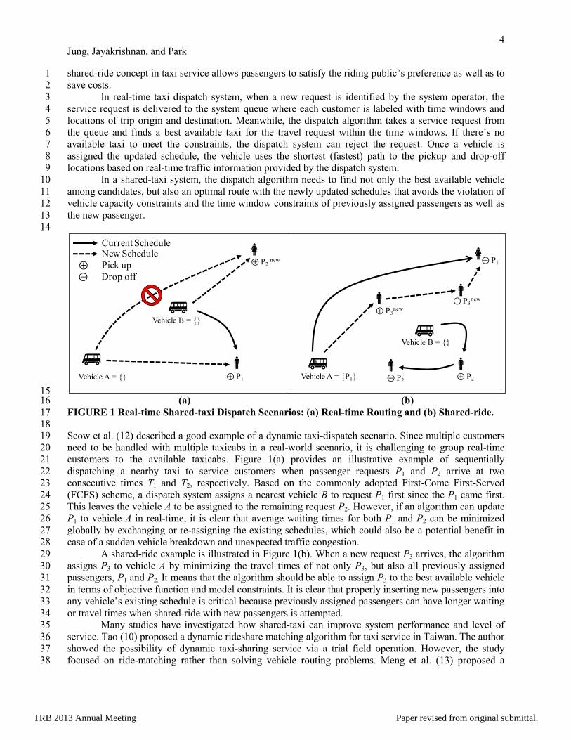
FIGURE 1 Real-time Shared-taxi Dispatch Scenarios: (a) Real-time Routing and (b) Shared-ride. 17

18 Seow et al. (12) described a good example of a dynamic taxi-dispatch scenario. Since multiple customers 19

need to be handled with multiple taxicabs in a real-world scenario, it is challenging to group real-time 20

customers to the available taxicabs. Figure 1(a) provides an illustrative example of sequentially 21

dispatching a nearby taxi to service customers when passenger requests P1 and P2 arrive at two 22

consecutive times T1 and T2, respectively. Based on the commonly adopted First-Come First-Served 23

(FCFS) scheme, a dispatch system assigns a nearest vehicle B to request P1 first since the P1 came first. 24

This leaves the vehicle A to be assigned to the remaining request P2. However, if an algorithm can update 25

P1 to vehicle A in real-time, it is clear that average waiting times for both P1 and P2 can be minimized 26

globally by exchanging or re-assigning the existing schedules, which could also be a potential benefit in 27

case of a sudden vehicle breakdown and unexpected traffic congestion. 28

A shared-ride example is illustrated in Figure 1(b). When a new request P3 arrives, the algorithm 29

assigns P3 to vehicle A by minimizing the travel times of not only P3, but also all previously assigned 30

passengers, P1 and P2. It means that the algorithm should be able to assign P3 to the best available vehicle 31

in terms of objective function and model constraints. It is clear that properly inserting new passengers into 32

any vehicle’s existing schedule is critical because previously assigned passengers can have longer waiting 33

or travel times when shared-ride with new passengers is attempted. 34

Many studies have investigated how shared-taxi can improve system performance and level of 35

service. Tao (10) proposed a dynamic rideshare matching algorithm for taxi service in Taiwan. The author 36

showed the possibility of dynamic taxi-sharing service via a trial field operation. However, the study 37

focused on ride-matching rather than solving vehicle routing problems. Meng et al. (13) proposed a 38

Vehicle A = {}

Vehicle B = {}

⊕ P1

Current Schedule

⊕ P2new

Vehicle A = {P1}

Vehicle B = {}

⊕ P2

⊕ P3new

⊖ P1

⊖ P3new

⊖ P2

New Schedule

⊕ Pick up

⊖ Drop off


5


Genetic Network Programming algorithm for a multiple-customer strategy for a taxi dispatch system and 1

showed that their Multi-Customer Taxi Dispatch System (MCTDS) can enhance the quality of the taxi 2

service within a grid-type artificial network including 25 intersections. Lee et al. (14) introduced a two-3

step taxi-pooling dispatch system and provided a sensitivity analysis of the system performance. That 4

study tackled the taxi-pooling problem for a feeder system that transport passengers to a metropolitan 5

rapid transit (MRT) station, which implied that the passenger destinations were limited to one point (a 6

many-to-one problem). 7

3. MODELING SHARED-TAXI DISPATCH ALGORITHMS 8

This chapter defines the objective functions and problem constraints. Then, three different algorithms for 9

shared-taxi are introduced and compared: (a) a Nearest Vehicle Dispatch (NVD) algorithm that is most 10

commonly used in real applications; (b) an Insertion heuristic (IS) that handles real-time passenger 11

requests in a fast and simple manner; and (c) a Hybrid Simulated Annealing (HSA) that assign passengers 12

efficiently and dynamically to available vehicles. 13

Model Constraints and Objectives 14

Compared to conventional DRT systems that usually have been focusing either pickup or dropoff as 15

passenger time-window constraints, passengers’ concerns in shared-taxi will be how long they wait for a 16

service and how long detour they have by allowing their rides with other passengers because taxi trips are 17

characterized as an instantaneous short trip in urban areas. Consequently, three types of constraints are 18

introduced: (1) vehicle capacity; (2) maximum passenger wait time; and (3) maximum detour factor. 19

Differently from a many-to-one problem, a vehicle needs to pick up and drop off passengers continually 20

without service cycle. Thus checking the number of available seats among the vehicles’ schedules is 21

essential when inserting a new schedule. It is noted that in practical dynamic vehicle routing, trip requests 22

can be rejected by service providers due to the limited number of vehicles, especially when the passengers 23

have time windows or maximum detour constraints. In this paper, passengers are considered not to wait 24

longer than a certain period. The time window for passenger waiting time (e.g., 15 min) is capable of 25

strictly preventing the indefinite deferment of unassigned passengers. The final constraint is on a 26

maximum detour factor guaranteeing an upper bound on the passengers’ in-vehicle traveling time 27

between their origins and destinations. This constraint prevents excessive detours caused by too many 28

passengers being assigned on a vehicle trip. The maximum detour factor thus has an important impact in 29

determining the level of service. 30

Two types of objectives are considered: (1) Minimizing passenger waiting times and detours 31

caused by ride sharing; (2) Maximizing system profit from accepting passengers selectively based on the 32

current schedule. Since each algorithm could have different numbers of delivered passengers during 33

simulation with the objective function (1), scoring is proposed based on the number of delivered and 34

rejected requests, average waiting time, and average travel time. When scores are found in this way, a 35

lower score (cost) indicates better performance. 36

37

(1) 38

39

: Penalty value for a dropped request, 7200 sec 40

: A set of rejected requests during the simulation 41

: A set of completed requests during the simulation 42

: Travel time of passenger

43

: Waiting time of passenger

44

45

The system profit is proposed based on the profit found from vehicle operating cost (which in turn is 46

based on vehicle distance traveled) and service revenue (which is based on the number of delivered 47

passengers). In common taxi fare collection schemes, the fare starts at a basic flat fare with additional 48


6


charges applying according to distance traveled and time waited. As the study context is an urban area in 1

South Korea, the relevant fare structure in this study is as per the following three components found in 2

general for taxi fare in South Korea. 3

4

Basic fee: This basic fare covers the first two kilometers. 5

Per mile (or kilometer) charge: An additional charge is applied every 144 meters. 6

Waiting charge: If the taxi speed drops below 15 km/hour, an additional charge is added every 35 7

seconds. 8

9

In this study, we assume that the service revenue consists of two parts: fixed revenue and distance based 10

revenue. The operating cost can be obtained using the vehicle distance traveled, as follows. In this case, a 11

higher value indicates better performance. 12

13

(2) 14

15

: Fixed revenue (basic fare, 2000) 16

: Weight of distance based revenue, 1.0 17

: Weight of vehicle operating cost, 0.4 18

: Passenger door-to-door distance excluding the basic fare distance 19

: Vehicle distance traveled (km) 20

Nearest Vehicle Dispatch 21

Nearest Vehicle Dispatch (NVD) is the most widely employed strategy in current on-line taxi dispatch 22

systems with single customer group. NVD has the following two steps. In step 1, when a new passenger 23

request arrives, the algorithm seeks a geographically nearest available vehicle from the passenger’s origin 24

location so as to provide quick and efficient response times. Checking feasible time windows is carried 25

out at step 1. Once a nearest vehicle is selected, an optimal schedule is found at step 2 by assuming that 26

the vehicle’s pickup and delivery schedule can be independently optimized (similar to the driver or an in-27

vehicle computer doing that) based on the current location and the existing schedule. Since this greedy 28

algorithm only considers reaching the passenger with the shortest distance possible, it doesn’t need a 29

complicated dispatch algorithm. However, passengers could necessarily detour because the algorithm 30

doesn’t consider existing schedules, the time spent by passengers on board, or the trip origins and 31

destinations of those passengers. 32

Insertion Heuristic 33

While NVD searches only for a nearest feasible vehicle to assign a new passenger, Insertion heuristic (IS) 34

compares all feasible vehicles to find a best available vehicle for its objective. Although this study 35

focuses on a many-to-many vehicle routing problem, the proposed Insertion heuristic is based on a First-36

Come First-Served (FCFS) policy in which a new request is considered individually and independently 37

from other new requests. The proposed IS has four steps as follows if the objective is to minimize waiting 38

times and detours: (1) Each passenger trip is identified by its origin and destination; (2) Collect available 39

vehicles to insert a new trip request in the corresponding service area; (3) Select a vehicle by minimizing 40

service waiting time and travel time of the new passengers as well as the existing passengers; (4) Update 41

the vehicle schedule with a new request. The detailed procedure is following: 42

43

1. A new passenger request, zi (i I ) comes in, and pickup and delivery locations and the number 44

of passengers in the group are identified. 45

2. Once the system searches for a vehicle j among all available vehicles J, (j J), it confirms 46

whether the constraints meet or not with new pickup and dropoff events, ei,pick

and ei,drop

, 47

associated with zi. If they are acceptable, the incremental cost ICj (ei,pick

, ei,drop

) based on its 48


7


current schedule K, (k K) is calculated to determine the optimal vehicle. In the same procedure, 1

it searches for the best insertion positions for the new events among the current schedules Ej by 2

calculating the expected waiting and travel time of the new passenger as well as previously 3

assigned passengers. The best vehicle is updated with the total cost Cj found and corresponding 4

insertion positions for ei,pick

and ei,drop

. 5

3. If there are no more available vehicles to consider, the dispatch algorithm assigns the passenger to 6

the vehicle with the minimum incremental cost, ICj. Otherwise, the passenger request is rejected 7

due to the constraints. 8

4. Once the best vehicle is determined, the pickup and delivery schedules (ei,pick

and ei,drop

) are 9

inserted into the optimal position among the existing schedules of the vehicle. 10

5. Dispatch the vehicle following the schedule to serve the new passenger. 11

12

(3) 13

(4) 14

(5) 15

16

: Waiting time of the previously assigned passenger with

17

: Waiting time of the new passenger zi with the m-th pickup order (0 < m) 18

: Travel time of the previously assigned passenger with ek 19

: Travel time of the new passenger zi with the n-th dropoff order (m < n) 20

21

The Cj in (3) can be calculated based on the vehicle’s current schedule Ej. Waiting time for passengers 22

can be obtained with pickup events whereas travel time can be calculated with delivery events. ICj in (5) 23

includes two terms respectively: (a) The total cost calculated for the updated schedule including ei,pick

and 24

ei,drop

; (b) The total cost calculated for the current schedule of vehicle j. Note that since adding a new 25

schedule causes extra costs for a vehicle, the incremental cost should be always positive. The formulation 26

(4) returns not only the total cost, but also the optimal insertion positions for the new events. The cost 27

function can be replaced by the system profit in a similar manner, if needed. 28

The proposed insertion heuristic is fairly easy and straight-forward to implement, and shows 29

computational efficiency, but it has limitations on dynamic pickup and delivery operations. The primary 30

limitation is that it has no dynamic schemes capable of re-optimizing vehicle schedules by shifting or 31

exchanging previously assigned passenger pickup and delivery schedules. Thus it should be expected that 32

it would normally achieve a sub-optimal solution. The problem of finding an optimal solution is however 33

not easy as the well-known combinatorial issues ensue. This leads us to developing an optimization 34

scheme that while still is heuristic, can reach near optimal solutions, as described next. 35

Hybrid Simulated Annealing 36

Simulated Annealing (SA), first suggested by Metropolis et al. (15) and defined by Kirkpatrick et al. (16) 37

is a generic probabilistic meta-heuristic, which is capable of finding an approximately accurate solution 38

for the global optimum of a complex system with a large search space. The name of Simulated Annealing 39

(SA) involves a technique such as heating and cooling of a material in annealing in metallurgy. It is 40

widely known that the heat treatment in metallurgy enables the property of material to change in its 41

hardness and strength. SA is a stochastic relaxation method based on an iterative procedure starting at an 42

initial “higher temperature” with the system in a known configuration, the word “temperature” being used 43

to give an intuitive connection to metallurgy. The iterative procedure of SA improves the cost function 44

until the current temperature cools down. At higher temperatures, the atoms are likely to become unstable 45

from the initial position, which means that the algorithm is allowed to have flexibility in searching the 46

feasible space, while at lower temperatures it has more chances to find improvement with local search 47


8


than the initial state (16). In comparison with NVD and IS, SA provides a systematic re-optimization 1

scheme to assign new requests as well as update existing vehicle schedules in real-time. 2

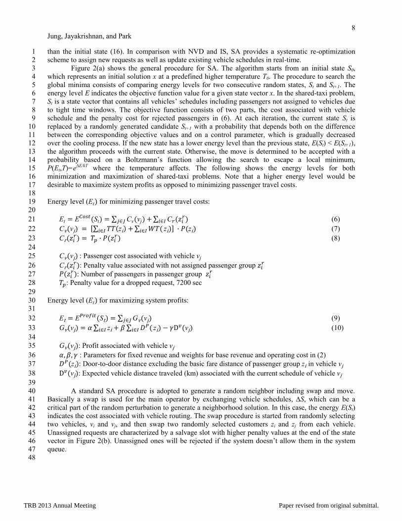
Figure 2(a) shows the general procedure for SA. The algorithm starts from an initial state S0, 3

which represents an initial solution x at a predefined higher temperature T0. The procedure to search the 4

global minima consists of comparing energy levels for two consecutive random states, St and St+1. The 5

energy level E indicates the objective function value for a given state vector x. In the shared-taxi problem, 6

St is a state vector that contains all vehicles’ schedules including passengers not assigned to vehicles due 7

to tight time windows. The objective function consists of two parts, the cost associated with vehicle 8

schedule and the penalty cost for rejected passengers in (6). At each iteration, the current state St is 9

replaced by a randomly generated candidate St+1 with a probability that depends both on the difference 10

between the corresponding objective values and on a control parameter, which is gradually decreased 11

over the cooling process. If the new state has a lower energy level than the previous state, E(St) < E(St+1), 12

the algorithm proceeds with the current state. Otherwise, the move is determined to be accepted with a 13

probability based on a Boltzmann’s function allowing the search to escape a local minimum, 14

P(Et,T)=e∆E/kT

where the temperature affects. The following shows the energy levels for both 15

minimization and maximization of shared-taxi problems. Note that a higher energy level would be 16

desirable to maximize system profits as opposed to minimizing passenger travel costs. 17

18

Energy level ( for minimizing passenger travel costs: 19

20

(6) 21

(7) 22

(8) 23

24

: Passenger cost associated with vehicle 25

: Penalty value associated with not assigned passenger group

26

: Number of passengers in passenger group

27

: Penalty value for a dropped request, 7200 sec 28

29

Energy level ( for maximizing system profits: 30

31

(9) 32

(10) 33

34

: Profit associated with vehicle 35

: Parameters for fixed revenue and weights for base revenue and operating cost in (2) 36

: Door-to-door distance excluding the basic fare distance of passenger group in vehicle 37

: Expected vehicle distance traveled (km) associated with the current schedule of vehicle 38

39

A standard SA procedure is adopted to generate a random neighbor including swap and move. 40

Basically a swap is used for the main operator by exchanging vehicle schedules, ∆S, which can be a 41

critical part of the random perturbation to generate a neighborhood solution. In this case, the energy E(St) 42

indicates the cost associated with vehicle routing. The swap procedure is started from randomly selecting 43

two vehicles, vi and vj, and then swap two randomly selected customers zi and zj from each vehicle. 44

Unassigned requests are characterized by a salvage slot with higher penalty values at the end of the state 45

vector in Figure 2(b). Unassigned ones will be rejected if the system doesn’t allow them in the system 46

queue. 47

48


9


1

2 3

(a) 4 5

6 7

(b) 8 9

FIGURE 2 (a) Simulated Annealing Procedure and (b) System State Vector. 10 11

When inserting a new customer to the vehicle’s schedule, the existing vehicle schedules need to be 12

updated. A heuristic insertion algorithm is adopted to keep the individual vehicle’s schedule optimized, 13

called Hybrid Simulated Annealing (HSA). One reason is that the validity of a newly generated neighbor 14

should be checked while generating a neighborhood solution because the swap and move operations can 15

generate infeasible solutions with the aforementioned random search. Unexpected infeasible solutions 16

would however cause a significant impact on system efficiency and solution accuracy. For this reason, 17

many types of SA applications combine a general SA procedure with another heuristic technique that 18

enables the search moves to be within the feasible space. Searching a random candidate, the grayed part 19

in Figure 2(a), can be replaced by the IS algorithm proposed in the previous section due to the 20

characteristics of the shared-taxi problem with constraints such as vehicle capacity and time windows. 21

SA starts with parameters, iteration Iiter, initial temperature T0, final temperature Tc, cooling rate 22

Rc, and Boltzmann constant K. Iiter denotes the number of iterations at a particular temperature. Setting the 23

New Temperature, T(t)

Initial Energy State

E0(S0), T0

t = t + ∆t

Random perturbation

to search a system state, St

Energy, Et = E(St)

Et < Et - ∆t

No

Converged?No

Yes

Acceptance Probability

P(Et , T)

Random r [0,1]

r < P(Et , T)

Accept St

St ← t

Reject St

St ← St - ∆t

Yes No

Final results

1 Unassigned Pax

5

+

5

-

6

+

6

-

3

+

3

-

1

+

4

+

4

-

1

-

10

+

7

+

10

-

7

-

2 3 4

2 8 9

+ -Pickup Dropoff


10


number of iteration is critical for a multiple vehicle routing problem because a higher number of iteration 1

provides a higher opportunity to move around the search space expanded as the number of vehicles 2

increases. An alternative is to change the number of iterations dynamically, depending on a temperature. 3

For example, a large number of iterations are required to thoroughly explore the local optimum. On the 4

other hand, the number of iterations is not necessarily large at higher temperatures. Setting the 5

temperature plays a critical role in acceptance probability, which means that the value of initial 6

temperature depends on the scale of the cost of a problem-specific objective function. The initial 7

temperature should not be high enough that the algorithm simply conducts a random search, causing 8

excessive computation time. A preliminary search can be used to estimate the initial temperature by 9

calculating an average objective increase, in formula (11), where is a desired average increase of 10

acceptance probability. According to Crama and Schyns (17), usually [0.8, 0.9], and Rc and K are 11

normally set with r ∈ [0.80, 0.99] and k ∈ [0.1, 1.0], respectively. 12

13

(11) 14

15

Note that the selection of parameters including the number of iterations and temperature might not only 16

affect the quality of the solution, but also has significant influence on the algorithm’s run-time. It is 17

known that a good initial solution improves the quality of solution as well as the convergence time. To 18

generate a good feasible solution for SA in real-time scheduling, other meta-heuristic techniques can be 19

used with combination of parallel computing techniques (18). 20

4. SIMULATION IMPLEMENTATION 21

Simulation Design 22

A shared-taxi simulator is written in Microsoft Visual C++, which is capable of implementing various 23

types of algorithms and visualizing all simulation elements (e.g., tracking vehicles and passengers) as in 24

Figure 3(b). The simulator imports digital maps designed for map display, geo-coding, and includes faster 25

vehicle routing with realistic roadway attributes such as road categories, turning prohibition, one-way, 26

posted speed, numbers of lanes, link lengths, and link shapes. For a simulation in urban area, Seoul area is 27

abstracted from the national transportation network, and it contains 8,382 links and 6,321 nodes. The link 28

shapes used here are as per the transportation network in the KOTI (Korea Transport Institute) regional 29

transportation planning model. 30

For taxi demand generation, the demand data used are as in the KOTI regional transportation 31

planning model. As of 2011, the trip demand consists of auto, bus, subway, rail, taxi, and other types of 32

demands, which covers Seoul with a total of 560 zones. Under the usual assumption of spatial uniformity 33

of demand around a zone centroid, point-to-point dynamic taxi demands are randomly generated in 34

accordance with destination probabilities from the taxi demand table of each centroid. The real-time 35

service requests arrive according to a Poisson process in a temporal manner. Figure 3(a) shows the trip 36

length distribution of 12,000 trip requests generated based on the taxi demand table with the minimum 37

trip length, 1.5 km for the taxi service. It shows that majority of trip demands are within 10 km. The 38

average trip length is 6.3 km and the expected door-to-door travel time 13.3 min under the assumption 39

that vehicles can travel at 60-90% of the posted speeds on the network. 40


11


1 (a) (b) 2 3

FIGURE 3 (a) Trip distribution of requests and (b) Shared-taxi Simulator with Seoul Network. 4 5

Simulation Scenarios 6

According to the Seoul Taxi Association, a total of 72,000 taxi licenses are registered including owner-7

driver taxis, and a total fleet of 40,000 vehicles are actually operated as of 2011. A total of 600 service 8

vehicles are considered in the simulation, which is equivalent to 1.5% of the total number of vehicles 9

operated in Seoul. The initial vehicle positions are randomly generated over the simulation area. We 10

consider 4-seater taxicabs for shared rides. As for demand levels, four different demand levels (9,000, 11

12,000, 15,000, and 18,000 requests equivalent to 3.7, 5.0, 6.3, and 7.5 requests/km2-hr) are considered 12

based on the request pool generated in Table 1. The total simulation time is set to 4 hours including 30 13

min as a warm-up period. An average of 1-min boarding and alighting times are assumed for each 14

passenger, with a normal distribution N(1.0, 1.0). Three different algorithms, namely, NVD, IS, and HSA 15

are tested. For HSA, 60 sec is considered as the period for successive re-optimization. We set the 16

maximum 6,000 iterations at each annealing temperature and the lowest temperature 0.2. 17

Two types of customer policies are considered. First, Single Customer Operation (SCO) is the 18

traditional taxi service without ride sharing. Each passenger trip request is matched to the best available 19

empty vehicle according to the objective function. Multiple Customer Operation (MCO) allows taxicabs 20

to pick up multiple customers whose origins and destinations could be different, but minimizing their 21

waiting time and travel time or maximizing profits as long as the vehicle has vacancy. 22

23

TABLE 1 Simulation Scenarios 24

Shared-taxi simulation

Shared Taxi settings

Service area (km2)

Simulation time (hours)

Warm up (hours)

Number of service vehicles

Vehicle capacity (passengers/vehicle)

Maximum waiting time

Maximum detour factor

Operation types1

Demand and Algorithm settings

Demand levels (thousand requests/4-hour)

Routing algorithms2

605

4

0.5

600

1 and 4

15 min

2.0

SCO, MCO

9, 12, 15, and 18

NVD, IS, and HSA 1: SCO: Single Customer Operation, MCO: Multiple Customer Operation 25

0

0.5

1

1.5

2

2.5

1 4 7 10 13 16 19 22 25 28 31 34 37 40

Trip

s (t

ho

usa

nd

)

Trip Distance (km)


12


2: NVD: Nearest Vehicle Dispatch, IS: Insertion heuristic, HSA: Hybrid Simulated Annealing 1

5. SIMULATION RESULTS 2

Two performance measures are introduced in order to compare the system efficiency and performance, 3

Level-of-Service (LOS) index ( ) and Ride-time index ( ), which are discussed by Black (19) is adopted 4

to compare the system efficiency in shared-ride transportation systems. Note that these indices may be a 5

little misleading, as lower values indicate better. The door-to-door ride time in (12, 13) is the travel time 6

when no other passengers are picked up or dropped enroute (i.e., equivalent to the time for driving a 7

personal auto) given the same network conditions. 8

9

10

11

Minimizing Wait and Travel Times 12

Figure 4 shows performance measures of 4-seater taxi with passenger travel cost minimization. Regarding 13

passenger delivery, HSA apparently performs better than other two algorithms. However, when the 14

passenger demand stays lower levels (9,000 and 12,000 requests), there’s no significant difference 15

between IS and HSA in terms of passenger delivery and reject in Figure 4(a) and 4(b). As expected, NVD 16

performs worst due to the lack of optimality whereas both IS and HSA consider passengers’ waiting and 17

traveling time. NVD assigns greedily passengers to the nearest vehicles to minimize passenger waiting 18

time without any consideration of passengers’ origins and destinations, so it is clearly seen that the LOS 19

index of NVD shows lowest among other algorithms although the ride-time index of NVD shows highest 20

even with lower demand levels in Figure 4(c) and 4(d). 21

In table 2, average waiting times remain from six to twelve minutes, which are far below the 22

maximum waiting time constraint, 900 sec. That is explained by another bound constraint with maximum 23

detour factor, 2.0. It is also important to note that ride-time index can be slightly over 2.0 because 24

passengers’ boarding and alighting times are assumed randomly during the simulation. For instance, 25

excessive longer boarding or alighting times of one passenger will affect the travel time of other 26

passengers on board in shared-ride operation. At higher levels of passenger requests, the ride-time indices 27

of IS and HSA are almost 2.0. The average vehicle distance traveled decreases as the demand increases in 28

IS and HSA, which is very consistent with increased vehicle loads. 29

Figure 4(e) and 4(f) show the objective function cost comparisons of the simulation results. The 30

normalized costs by the total number of requests are also given. Apparently, HSA outperforms than both 31

NVD and IS. Although there’s no difference between IS and HSA at the lowest demand level, IS shows 32

higher costs similar to NVD as the demand level increases. Since IS simply finds the best vehicle to insert 33

a new passenger at a time - not considering the all passengers at the same time - the deterioration of 34

system performance is unavoidable compared with HSA that periodically optimizes the entire vehicle 35

schedules, which can’t be achieved by a simple heuristic solution. It is also noted that the penalty value 36

(7200 sec) for rejected requests in HSA can impact significantly on both the number of delivered 37

passengers and the quality of service simultaneously. 38


13


1

2 (a) (b) 3

4

5 (c) (d) 6

7

8 (e) (f) 9

10

FIGURE 4 Performance measures (Minimizing Cost with MCP): (a) Number of Delivered 11

Passengers, (b) Number of Rejected Requests, (c) LOS Index, (d) Ride time Index, (e) Total Cost, 12

and (f) Normalized Cost. 13 14

Maximizing Profit 15

When applying the profit maximization for algorithms, HSA algorithm tends to accepts passengers’ 16

requests selectively to maximize its objective. Figure 5 shows the system performance. Different from the 17

previous results, the numbers of delivered and rejected passengers in Figure 5(a) and 5(b) are very similar 18

over three algorithms. In Figure 5(e), both IS and HSA shows the similar profits at the lowest demand 19

compared to the number of service vehicles while the profit of NVD is far below of IS and HSA. As 20

7

8

9

10

11

12

13

9k 12k 15k 18k

De

live

red

Pas

sen

gers

(k)

Demand Levels

NVD

IS

HSA

0

1

2

3

4

5

6

9k 12k 15k 18k

Re

ject

ed r

eq

ue

sts

(k)

Demand Levels

NVD

IS

HSA

0.0

0.2

0.4

0.6

0.8

1.0

1.2

1.4

9k 12k 15k 18k

LOS

Ind

ex

Demand Levels

NVD

IS

HSA

1.0

1.2

1.4

1.6

1.8

2.0

2.2

2.4

9k 12k 15k 18k

Rid

e T

ime

Ind

ex

Demand Levels

NVD

IS

HSA

2

4

6

8

10

12

14

16

9k 12k 15k 18k

Tota

l co

st (t

ho

usa

nd

ho

urs

)

Demand Levels

NVD

IS

HSA

0.3

0.4

0.5

0.6

0.7

0.8

0.9

1.0

1.1

9k 12k 15k 18k

Co

st (n

orm

aliz

ed

)

Demand Levels

NVD

IS

HSA


14


passenger demand increases, the profit with HSA keeps increasing gradually while the profit with IS stays 1

constant after the demand level, 15,000. This can be explained on the basis of the optimization concept of 2

HSA. The HSA is capable of re-optimizing vehicle schedules by shifting or exchange previously assigned 3

passengers’ schedules. The same patterns are observed in the cost minimization in the previous section, 4

but applying the penalty (7200 sec) in HSA for real-time passenger delivery system where rejecting 5

passengers is necessary, might cause additional impacts on system performance unless the penalty values 6

are carefully evaluated, as mentioned earlier, while NVD and IS don’t reject any of requests as long as the 7

requests meet the constraints. When comparing passenger door-to-door distances, it is shown that HSA 8

algorithm clearly tends to accept passengers who have longer travel distance in the profit maximization 9

(average door-to-door trip length of delivered passengers, 6.4 km/request) than in the cost minimization 10

(5.9 km). This is because vehicles would have a higher chance to fully utilize its available seats with 11

longer passenger trips rather than with shorter trips. 12

In table 2, the average vehicle distance travel with IS and HSA (60 - 85 km) with the profit 13

maximization strategy are significantly lower than the values (83 - 95 km) obtained with the cost 14

minimization in the same table. It is reasonable that the dispatch algorithm tries to maximize system profit 15

(equivalent to minimize operating costs), directly linked to vehicle distance traveled. It is noted that the 16

cost minimization strategy not only minimizes the passenger waiting time and travel time, but also tries to 17

maximize the passenger delivery as long as the incremental cost is less than the predefined penalty, while 18

the focus of the profit maximization rejects requests is to achieve a higher system profit without any 19

consideration of passenger delivery. 20


15


1

2 (a) (b) 3

4

5 (c) (d) 6

7

8 (e) (f) 9

10

FIGURE 5 Performance measures (Maximizing profit with MCO): (a) Number of Delivered 11

Passengers, (b) Number of Rejected Requests, (c) LOS Index, (d) Ride time Index, (e) Total Profit, 12

and (f) Normalized Profit. 13 14

15

6

7

8

9

10

11

12

9k 12k 15k 18k

De

live

red

Pas

sen

gers

(k)

Demand Levels

NVD

IS

HSA

0

1

2

3

4

5

6

9k 12k 15k 18k

Re

ject

ed R

eq

ue

sts

(k)

Demand Levels

NVD

IS

HSA

0.0

0.2

0.4

0.6

0.8

1.0

1.2

1.4

9k 12k 15k 18k

LOS

Ind

ex

Demand Levels

NVD

IS

HSA

1.0

1.2

1.4

1.6

1.8

2.0

2.2

2.4

9k 12k 15k 18k

Rid

e T

ime

Ind

ex

Demand Levels

NVD

IS

HSA

15

20

25

30

35

40

45

50

55

9k 12k 15k 18k

Tota

l Pro

fit

(th

ou

san

d)

Demand Levels

NVD

IS

HSA

2.0

2.5

3.0

3.5

4.0

4.5

5.0

5.5

6.0

9k 12k 15k 18k

Pro

fit

(no

rmal

ize

d)

Demand Levels

NVD

IS

HSA


16


1

TABLE 2 Detailed performance measures with MCO 2

Minimize Cost Maximize Profit

Vehicle Routing Schemes NVD IS HSA IS HSA

9,000-request

Total delivered passengers (requests)

Average wait time home (min)

Average passenger travel time (min)

Level-of-Service index

Ride-time index

Rejected passengers (requests)

Average vehicle load (passengers/veh)

Average vehicle dist. traveled (km)

7,146

6.55

21.49

0.54

1.76

12

1.61

78.09

7,551

8.74

15.04

0.67

1.15

6

0.94

92.81

7,586

8.04

15.01

0.61

1.14

4

0.93

88.31

7,211

9.44

24.03

0.75

1.91

66

1.57

60.92

7,140

9.69

23.75

0.75

1.83

225

1.47

62.41

12,000-request





Ride-time index




8,830

8.85

23.82

0.76

2.04

601

2.44

84.27

9,679

9.79

20.02

0.78

1.60

100

1.82

88.07

9,972

9.83

18.06

0.76

1.40

27

1.54

87.65

8,952

10.36

24.93

0.84

2.01

814

2.15

76.41

8,704

10.84

25.50

0.81

1.91

1,195

1.94

74.74

15,000-request





Ride-time index




9,724

9.86

24.50

0.85

2.12

2,451

2.78

85.95

10,392

10.61

22.92

0.88

1.90

1,837

2.53

85.99

11,292

11.27

20.85

0.90

1.67

1,136

2.14

83.88

9,996

10.74

25.50

0.88

2.08

2,418

2.56

83.05

9,842

11.47

27.12

0.84

2.00

2,762

2.35

82.19

18,000-request





Ride-time index




10,284

10.50

24.74

0.91

2.14

4,745

2.92

85.85

10,689

11.06

23.57

0.94

2.00

4,377

2.77

85.19

11,934

11.66

21.19

0.96

1.74

3,382

2.35

83.12

10,453

11.14

25.43

0.93

2.12

4,686

2.80

84.58

10,270

11.96

28.08

0.87

2.03

5,075

2.57

84.09

3

Benefits of Shared-taxi 4

Another simulation is performed to investigate the benefit of shared-taxi with the comparison between 5

SCO and MCO in Figure 6. SCO allows only one customer group in a taxi at any time during the service 6

period. There could be two different strategies for the scheduling of single customer vehicles. The first 7

strategy is that the new customers can be assigned only to idling vehicles with no current schedules while 8

the second is that new customers can be assigned to any vehicles satisfying the associate time constraints. 9


17


For example, in the second strategy a new schedule could be updated to a vehicle even before the vehicle 1

has finished the current schedule of the passenger on board. From preliminary simulation runs, it was 2

found that the first strategy delivers 25% less number of passengers, but it shows smaller waiting times at 3

home compared to the second strategy. In this simulation, the second strategy is employed due to its 4

similarity in the assumption used in the shared-taxi operation. The cost minimization scheme is applied 5

because the study focuses on the number of delivered passengers and their travel times. 6

SCO and MCO are compared using HSA in Figure 6. Significantly notable increases can be seen 7

in the number of delivered passengers with MCO in Figure 6(a). At the highest demand level, MCO 8

shows about 4,000 more delivered passengers than SCO. The number of rejected passengers in MCO 9

stays at the lower level at the lower demand levels, and then starts increasing, indicating that the shared-10

ride system rarely drops passengers given the fleet size and passenger demands. It is very interesting that 11

LOS index with MCO is lower than with SCO in Figure 6(c). It can be explained that MCO has a higher 12

probability to pick up passengers. Consequently the passengers might wait for a shorter time than the case 13

of SCO in which a vehicle can go to pick up a passenger only after dropping off the passenger on board. 14

Ride-time index with MCO keeps increasing as the trip requests increase, but stay below 2.0 due to the 15

proposed constraint in Figure 6(d). It is reasonable that the ride-time indices with SCO stay at the same 16

level across all algorithms and scenarios, at a value of 1.0, because the vehicles are not allowed to be in 17

shared-ride operation. 18

As for a combined index from summing both ride-time and LOS indices, MCO shows a lower 19

value than SCO at the lowest demand level. This denotes that the proposed shared-ride system could not 20

only serve more passengers, but also provides better quality of service (QoS) by allowing ride-sharing at 21

certain demand levels. Most importantly, MCO has more than tripled its average vehicle load than SCO 22

indicating higher vehicle utilization compared to SOC. However, the number of delivered passengers 23

does not increase as much. It implies that the average vehicle load should be carefully considered as a 24

performance indicator because it could include side effects related to passenger trip lengths. It should be 25

noted however that the passengers’ convenience and comfort is not the focus in this study. Those are 26

aspects which significantly affect the demand, but are beyond the scope of this study that focuses on the 27

operational efficiency. Regarding vehicle travel distance in Figure 6(f), MCP shows less average travel 28

distance (85.7 km) than SCO (97.1 km), which can also expect less vehicle operating costs than SCO. 29


18


1

2 (a) (b) 3

4

5 (c) (d) 6

7

8 (e) (f) 9

10

FIGURE 6 Performance Comparison between SCO and MCO: (a) Number of Delivered Passengers, 11

(b) Number of Rejected Requests, (c) LOS Index, (d) Ride time Index, (e) Average Vehicle Load 12

(passengers/vehicle), and (f) Average Vehicle Distance Moved (km) during the simulation. 13

14

6. CONCLUSION 15

Taxi is a convenient and fast and flexible transportation method in urban areas. A dynamic shared-taxi 16

system is proposed with three types of taxi dispatch algorithms. It is assumed that all vehicles can 17

optimize their schedule at the individual vehicle level with given pickup and delivery schedules. It is 18

shown that HSA systematically optimizes the entire schedules of the vehicles in real-time, which is not 19

possible with eight NVD or IS in this study. From the simulation study, it is seen that the proposed 20

0

2

4

6

8

10

12

14

9k 12k 15k 18k

De

live

red

Pas

snge

rs (k

)

Demand Levels

SCO MCO

0

2

4

6

8

10

12

14

9k 12k 15k 18k

Re

ject

ed P

assn

gers

(k)

Demand Levels

SCO MCO

0.4

0.6

0.8

1.0

1.2

1.4

1.6

1.8

2.0

9k 12k 15k 18k

LOS

Ind

ex

Demand Levels

SCO MCO

0.4

0.6

0.8

1.0

1.2

1.4

1.6

1.8

2.0

9k 12k 15k 18k

Rid

e T

ime

Ind

ex

Demand Levels

SCO MCO

0.5

0.7

0.9

1.1

1.3

1.5

1.7

1.9

2.1

2.3

2.5

9k 12k 15k 18k

Avg

. Ve

hic

le L

oad

Demand Levels

SCO MCO

70

75

80

85

90

95

100

9k 12k 15k 18k

Avg

. Ve

hic

le D

ista

nce

Mo

ve

Demand Levels

SCO MCO


19


shared-taxi system has potential in improving the system performance compared to the conventional form 1

of taxi service. However, increasing travel time of passengers (vehicle ride time) is inevitable, and the 2

demand impacts need to be investigated within the given detour constraint. 3

In this study, we assumed that all passengers are willing to share their rides with other passengers 4

and the simulation results show great potentials that ride-sharing can reduce the taxi fare by improving the 5

system productivity. However, in real practice, not all passengers want to share their ride. Considering 6

that many passengers are still not allowing ride-sharing for their comfort or convenience, it should be 7

addressed that the proposed shared-taxi model can deal with this issue depending on the passengers’ 8

different willingness (e.g., individual preference for maximum waiting time and detour) towards ride-9

sharing in real-time. Moreover, taxis would have greater capability for it than other transportation means 10

because individual vehicles can dynamically switch their operation between single and multiple customer 11

schemes. The proposed shared-taxi concept will be applied to increase the efficiency of EV (Electric 12

Vehicle) taxi operation, which usually suffers from limitations by short driving range and battery 13

charging. Also, the author want to emphasize that the share-ride system proposed in this study can be 14

easily converted to a real-time shared-van (shuttle) service. 15

7. ACKNOWLEDGEMENT 16

This project is funded by the Korea Transport Institute (KOTI), as part of “Electric Vehicle 2011”, 17

initiated by the National Research Council for Economics, Humanities and Social Science, South Korea. 18

19

20


20


REFERENCES 1

1. Dial, R. B. (1995). Autonomous Dial-a-Ride Transit Introductory Overview. Transportation Research, 2

Vol. 3C, No. 5, pp. 261-275. 3

2. Cortés, C. E. and Jayakrishnan, R. Design and Operational Concepts of High-Coverage Point-to-Point 4

Transit System. In Transportation Research Record: Journal of the Transportation Research Board, 5

No. 1783, National Research Council, Washington, D.C., 2002, pp. 178-187. 6

3. Jung, J. and Jayakrishnan, R. High Coverage Point-to-Point Transit: Study of Path-Based Vehicle 7

Routing Through Multiple Hubs. In Transportation Research Record: Journal of the Transportation 8

Research Board, No. 2218, Transportation Research Board of the National Academies, Washington, 9

D.C., 2011, pp.78-87. 10

4. Zimride. http://www.zimride.com. Accessed July 17, 2012. 11

5. Avego. http://www.avego.com. Accessed July 17, 2012. 12

6. SideCar. http://www.side.cr. Accessed July 17, 2012. 13

7. Cervero, R. Paratransit in America: Redefining Mass Transportation. Praeger Publishers, Westport, 14

Conn., 1997. 15

8. Uber. http://www.uber.com. Accessed July 17, 2012. 16

9. Split-it. http://www/split-it.sg. Accessed July 31, 2012 17

10. Tao, C. C. Dynamic Taxi-sharing Service Using Intelligent Transportation System Technologies. 18

Wireless Communications, Networking and Mobile Computing, 2007, International Conference on. 19

21-25 Sep, 2007, pp. 3209-3212. 20

11. Tsukada, N. and Takada, K. Possibilities of the Large-Taxi Dial-a-ride Transit System Utilizing GPS-21

AVM, Journal of Eastern Asia Society for Transportation Studies, EASTS, Bangkok, Thailand, 2005, 22

pp. 1-10. 23

12. Seow, K. T., Dang, N. H., and Lee, D. H. A Collaborative Multiagent Taxi-Dispatch System. IEEE 24

Transactions on Automation Science and Engineering, Vol. 7, Issue 3, 2010, pp. 607-616. 25

13. Meng, Q. B., Mabu, S., Yu, L., and Hirasawa, K. A Novel Taxi Dispatch System Integrating a Multi-26

Customer Strategy and Genetic Network Programming. Journal of Advanced Computational 27

Intelligence and Intelligent Informatics, Vol. 14, No. 5, 2010, pp. 442-452. 28

14. Lee, K. T., Lin, D. J., and Wu, P. J. Planning and Design of a Taxipooling Dispatch System. In 29

Transportation Research Record: Journal of the Transportation Research Board, No. 1930, 30

Transportation Research Board of the National Academies, Washington D.C., 2005, pp. 86-95. 31

15. Metropolis, N., Rosenbluth, A. W., Rosenbluth, M. N., Teller, A. H., and Teller, E. Equations of state 32

calculations by fast computing machines. Journal of Chemical Physics, Vol. 21, No. 6, 1953, pp. 33

1087-1092. 34

16. Kirkpatrick, S., Gelatt, C. D., and Vecchi, M. P. Optimization by Simulated Annealing. Science, Vol. 35

220, No. 4598, 1983, pp. 671-680. 36

17. Crama, Y., and Schyns, M. Simulated annealing for complex portfolio selection problem. European 37

Journal of Operational Research. Vol. 150, Issue 3, 2003, pp. 546-571. 38

18. Janaki Ram, D., Sreenivas, T. H., and Ganapathy Subramaniam, K. Parallel Simulated Annealing 39

Algorithms. Journal of Parallel and Distributed Computing, Vol. 37, Issue 2, 1996, pp. 207-212. 40

19. Black, A. Urban Mass Transportation Planning. McGraw-Hill Series in Transportation. McGraw-Hill, 41

New York, 1995. 42

43

44

45


Design and Modeling of Real-time Shared-Taxi Dispatch Algorithms

Documents

Transcript of Design and Modeling of Real-time Shared-Taxi Dispatch Algorithms