Design and manufacture of textile composites
492
Transcript of Design and manufacture of textile composites


i
Design and manufacture of textile composites

Related titles from Woodhead’s textile technology list:
3-D textile reinforcements in composite materials (1 85573 376 5)
3-D textile reinforced composite materials are obtained by applying highly productivetextile technologies in the manufacture of fibre preforms. The damage tolerance andimpact resistance are increased as the trend to delamination is drastically diminisheddue to the existence of reinforcements in the thickness direction. 3-D textilereinforcements in composite materials describes the manufacturing processes, highlightsthe advantages, identifies the main applications, analyses the methods for prediction ofmechanical properties and examines the key technical aspects of 3-D textile reinforcedcomposite materials. This will enable materials scientists and engineers to exploit themain features and overcome the disadvantages in relation to laminated compositematerials.
Green composites (1 85573 739 6)
Life cycle assessment is becoming increasingly important at every stage of a product’slife from initial synthesis through to final disposal, and a sustainable society needsenvironmentally safe materials and processing methods. With an internationallyrecognised team of authors, Green composites examines polymer composite productionand explains how environmental footprints can be diminished at every stage of the lifecycle. This book is an essential guide for agricultural crop producers, governmentalagricultural departments, automotive companies, composite producers and materialsscientists all dedicated to the promotion and practice of eco-friendly materials andproduction methods.
Bast and other plant fibres (1 85573 684 5)
Environmental concerns have regenerated interest in the use of natural fibres for amuch wider variety of products, including high-tech applications such as geotextiles,and in composite materials for automotive and light industry use. This new study coversthe chemical and physical structure of these natural fibres; fibre, yarn and fabricproduction; dyeing; handle and wear characteristics; economics; and environmentaland health and safety issues.
Details of these books and a complete list of Woodhead’s textile technology titlescan be obtained by:
∑ visiting our website at www.woodheadpublishing.com∑ contacting Customer Services (e-mail: [email protected];
fax: +44 (0) 1223 893694; tel.: +44 (0) 1223 891358 ext.30; address: WoodheadPublishing Limited, Abington Hall, Abington, Cambridge CB1 6AH, England)
ii

Published by Woodhead Publishing Limited in association with The Textile InstituteWoodhead Publishing LimitedAbington Hall, AbingtonCambridge CB1 6AHEnglandwww.woodheadpublishing.com
Published in North America by CRC Press LLC, 6000 Broken Sound Parkway, NW,Suite 300, Boca Raton FL 33487, USA
First published 2005, Woodhead Publishing Limited and CRC Press LLC© Woodhead Publishing Limited, 2005The authors have asserted their moral rights.
This book contains information obtained from authentic and highly regarded sources.Reprinted material is quoted with permission, and sources are indicated. Reasonableefforts have been made to publish reliable data and information, but the authors andthe publishers cannot assume responsibility for the validity of all materials. Neitherthe authors nor the publishers, nor anyone else associated with this publication, shallbe liable for any loss, damage or liability directly or indirectly caused or alleged to becaused by this book.
Neither this book nor any part may be reproduced or transmitted in any form or byany means, electronic or mechanical, including photocopying, microfilming andrecording, or by any information storage or retrieval system, without permission inwriting from the publishers.
The consent of Woodhead Publishing Limited and CRC Press LLC does not extendto copying for general distribution, for promotion, for creating new works, or forresale. Specific permission must be obtained in writing from Woodhead PublishingLimited and CRC Press LLC for such copying.
Trademark notice: Product or corporate names may be trademarks or registeredtrademarks, and are used only for identification and explanation, without intent toinfringe.
British Library Cataloguing in Publication DataA catalogue record for this book is available from the British Library.
Library of Congress Cataloging in Publication DataA catalog record for this book is available from the Library of Congress.
Woodhead Publishing Limited ISBN-13: 978-1-85573-744-0 (book)Woodhead Publishing Limited ISBN: 10-1-85573-744-2 (book)Woodhead Publishing Limited ISBN-13: 978-1-84569-082-3 (e-book)Woodhead Publishing Limited ISBN-10: 1-84569-082-6 (e-book)CRC Press ISBN 0-8493-2593-5CRC Press order number: WP2593
The publishers’ policy is to use permanent paper from mills that operate asustainable forestry policy, and which has been manufactured from pulpwhich is processed using acid-free and elementary chlorine-free practices.Furthermore, the publishers ensure that the text paper and cover board usedhave met acceptable environmental accreditation standards.
Project managed by Macfarlane Production Services, Markyate, Hertfordshire([email protected])Typeset by Replika Press Pvt Ltd, IndiaPrinted by T J International Limited, Padstow, Cornwall, England
iv

Contents
Contributor contact details ix
Introduction xiiiA C LONG, University of Nottingham, UK
1 Manufacturing and internal geometry of textiles 1S LOMOV, I VERPOEST, Katholieke Universiteit Leuven, Belgiumand F ROBITAILLE, University of Ottawa, Canada
1.1 Hierarchy of textile materials 11.2 Textile yarns 21.3 Woven fabrics 101.4 Braided fabrics 271.5 Multiaxial multiply non-crimp fabrics 351.6 Modelling of internal geometry of textile preforms 471.7 References 60
2 Mechanical analysis of textiles 62A C LONG, University of Nottingham, UK, P BOISSE, INSA Lyon,France and F ROBITAILLE, University of Ottawa, Canada
2.1 Introduction 622.2 In-plane shear 632.3 Biaxial in-plane tension 732.4 Compaction 882.5 References 107
3 Rheological behaviour of pre-impregnated textilecomposites 110P HARRISON and M CLIFFORD, University of Nottingham, UK
3.1 Introduction 1103.2 Deformation mechanisms 1113.3 Review of constitutive modelling work 1163.4 Characterisation methods 129
v

3.5 Forming evaluation methods 1373.6 Summary 1423.7 Acknowledgements 1423.8 References 143
4 Forming textile composites 149W-R YU, Seoul National University, Korea and A C LONG,University of Nottingham, UK
4.1 Introduction 1494.2 Mapping approaches 1494.3 Constitutive modelling approach 1554.4 Concluding remarks and future direction 1754.5 Acknowledgements 1784.6 References 178
5 Manufacturing with thermosets 181J DOMINY, Carbon Concepts Limited, UK, C RUDD, University ofNottingham, UK
5.1 Introduction 1815.2 Pre-impregnated composites 1815.3 Liquid moulding of textile composites 1875.4 References 196
6 Composites manufacturing – thermoplastics 197M D WAKEMAN and J-A E. MÅNSON, École Polytechnique Fédéralede Lausanne (EPFL), Switzerland
6.1 Introduction 1976.2 Consolidation of thermoplastic composites 1986.3 Textile thermoplastic composite material forms 2056.4 Processing routes 2176.5 Novel thermoplastic composite manufacturing routes 2336.6 Conclusions 2366.7 Acknowledgements 2366.8 References 237
7 Modeling, optimization and control of resin flowduring manufacturing of textile composites withliquid molding 242A GOKCE and S G ADVANI, University of Delaware, USA
7.1 Liquid composite molding processes 2427.2 Flow through porous media 2447.3 Liquid injection molding simulation 2477.4 Gate location optimization 254
Contentsvi
7.5 Disturbances in the mold filling process 2597.6 Active control 2687.7 Passive control 2747.8 Conclusion 2857.9 Outlook 2867.10 Acknowledgements 2887.11 References 288
8 Mechanical properties of textile composites 292I A JONES, University of Nottingham, UK and A K PICKETT,Cranfield University, UK
8.1 Introduction 2928.2 Elastic behaviour 2928.3 Failure and impact behaviour 3128.4 References 327
9 Flammability and fire resistance of composites 330A R HORROCKS and B K KANDOLA, University of Bolton, UK
9.1 Introduction 3309.2 Constituents – their physical, chemical, mechanical and
flammability properties 3329.3 Flammability of composite structures 3469.4 Methods of imparting flame retardancy to composites 3499.5 Conclusions 3599.6 References 360
10 Cost analysis 364M D WAKEMAN and J-A E MÅNSON, École Polytechnique Fédéralede Lausanne (EPFL), Switzerland
10.1 Introduction 36410.2 Cost estimation methodologies 36610.3 Cost build-up in textile composite applications 37410.4 Case study 1: thermoplastic composite stamping 38210.5 Case study 2: composites for the Airbus family 39610.6 Conclusions 40210.7 Acknowledgements 40210.8 References 402
11 Aerospace applications 405J LOWE, Tenex Fibres GmbH, Germany
11.1 Introduction 40511.2 Developments in woven fabric applications using
standard prepreg processing 406
Contents vii

11.3 Carbon fibre multiaxial fabric developments 40811.4 Improvement in standard fabric technology for
non-prepreg processing applications 41611.5 Braided materials 41711.6 Tailored fibre placement 41811.7 Preforming 41911.8 Repair of fabric components 423
12 Applications of textile composites in theconstruction industry 424J CHILTON, University of Lincoln, UK and R VELASCO,University of Nottingham, UK
12.1 Introduction 42412.2 Fibre reinforced polymers 42412.3 Membrane structures 42612.4 Case studies 42912.5 Future developments 43112.6 References 435
13 Textile reinforced composites in medicine 436J G ELLIS, Ellis Developments Limited, UK
13.1 Splinting material 43613.2 Walking support frame 43813.3 Bone plates 43913.4 General application 44113.5 Living composites 442
14 Textile composites in sports products 444K VAN DE VELDE, Ghent University, Belgium
14.1 Introduction 44414.2 Materials 44514.3 Design 44714.4 Production technology 44914.5 Applications 45014.6 Conclusion 45614.7 Acknowledgement 45614.8 References 456
Glossary 458
Index 463
Contentsviii

Contributor contact details
Introduction
Professor A.C. LongSchool of Mechanical, Materials andManufacturing EngineeringUniversity of NottinghamUniversity ParkNottingham NG7 2RDUK
Email: [email protected]
Chapter 1
Professor S. Lomov and Professor I.VerpoestKatholieke Universiteit LeuvenDepartment of MTMKasteelpark Arenberg 44B-3001, HeverleeBelgium
Email:[email protected]:[email protected]
Dr F. RobitailleFaculty of Engineering161 Louis PasteurRoom A306Ottawa, OntarioCanada K1N 6N5
Email: [email protected]
Chapter 2
Professor P. BoisseLaboratoire de Méchanique desContacts et des solidesLaMCoS, UMR CNRS 5514INSA de LyonBâtiment Jacquard27 Avenue Jean Capelle69621 Villeurbanne CedexFrance
Email:[email protected]
Professor A. C. LongSchool of Mechanical, Materials andManufacturing EngineeringUniversity of NottinghamUniversity ParkNottingham NG7 2RDUK
Email: [email protected]
Dr F. RobitailleFaculty of Engineering161 Louis PasteurRoom A306Ottawa, OntarioCanada K1N 6N5
Email: [email protected]
ix

Contributor contact detailsx
Chapter 3
Dr P. Harrison and Dr M. CliffordSchool of Mechanical, Materials andManufacturing EngineeringThe University of NottinghamUniversity ParkNottingham NG7 2RDUK
Tel: (44) (0)115 8466134Fax: (44) (0)115 9513800Email: [email protected]
Chapter 4
Professor A. C. LongSchool of Mechanical, Materials andManufacturing EngineeringUniversity of NottinghamUniversity ParkNottingham NG7 2RDUK
Email: [email protected]
Assistant Professor W-R. YuSchool of Materials Science andEngineeringSeoul National UniversitySan 56-1Shillim 9 dongKwanak-guSeoul 151-742Korea
Email: [email protected]
Chapter 5
Professor C. RuddSchool of Mechanical, Materials andManufacturing EngineeringUniversity of NottinghamUniversity ParkNottingham NG7 2RDUK
Email:[email protected]
Professor J. DominyCarbon Concepts LtdUnit A2, Lower Mantle CloseBridge Street Industrial EstateClay CrossDerbyshire S45 9NUUK
Email: [email protected]
Chapter 6 and 10
Dr M. D. Wakeman and ProfessorJ-A. E. MånsonLaboratoire de Technologiedes Composites et PolyméresÉcole PolytechniqueFédérale de LausanneLausanneSwitzerand
Tel: (41) 21 693 4281Email: [email protected]: [email protected]

Chapter 7
Dr A. Gokce and Professor S. G.AdvaniDepartment of MechanicalEngineeringUniversity of DelawareNewarkDE 19716USA
Email: [email protected]: [email protected]
Chapter 8
Dr I. A. JonesSchool of Mechanical, Materials andManufacturing EngineeringUniversity of NottinghamUniversity ParkNottingham NG7 2RDUK
Email: [email protected]
Professor A. K. PickettCranfield UniversitySchool of Industrial andManufacturing ScienceBuilding 61, CranfieldBedfordshire MK43 0ALUK
Tel: (44) (0)1234 754034Fax: (44) (0)1234 752473Email: [email protected]
Chapter 9
Professor A. R. Horrocks andDr B. K. KandolaCentre for Materials Research &InnovationUniversity of BoltonDeane RoadBolton BL3 5ABUK
Tel: +44 (0)1024 903831Email: [email protected]
Chapter 11
Dr J. LoweTenax Fibers GmbH & Co. KGKasinostrasse 19-2142 103 WuppertalGermany
Email: [email protected]
Chapter 12
Professor J. ChiltonLincoln School of ArchitectureUniversity of LincolnBrayford PoolLincoln LN6 7TSUK
Email: [email protected]
Dr R. VelascoSchool of the Built EnvironmentUniversity of NottinghamUniversity ParkNottingham NG7 2RDUK
Email:[email protected]
xiContributor contact details

Chapter 13
Mr J. G. Ellis, OBEEllis Developments LimitedThe ClocktowerBestwood VillageNottinghamNG6 8TQUK
Tel: 44 (0)115 979 7679Email: [email protected]
Chapter 14
Dr K. Van de VeldeGhent UniversityDepartment of TextilesTechnologiepark 907B-9052 Zwijnaarde (Ghent)Belgium
Email:[email protected]
Contributor contact detailsxii

Textile composites are composed of textile reinforcements combined with abinding matrix (usually polymeric). This describes a large family of materialsused for load-bearing applications within a number of industrial sectors. Theterm textile is used here to describe an interlaced structure consisting ofyarns, although it also applies to fibres, filaments and yarns, and most productsderived from them. Textile manufacturing processes have been developedover hundreds or even thousands of years. Modern machinery for processessuch as weaving, knitting and braiding operates under automated control,and is capable of delivering high-quality materials at production rates of upto several hundreds of kilograms per hour. Some of these processes (notablybraiding) can produce reinforcements directly in the shape of the finalcomponent. Hence such materials can provide an extremely attractivereinforcement medium for polymer composites.
Textile composites are attracting growing interest from both the academiccommunity and from industry. This family of materials, at the centre of thecost and performance spectra, offers significant opportunities for newapplications of polymer composites. Although the reasons for adopting aparticular material can be various and complex, the primary driver for theuse of textile reinforcements is undoubtedly cost. Textiles can be producedin large quantities at reasonable cost using modern, automated manufacturingtechniques. While direct use of fibres or yarns might be cheaper in terms ofmaterials costs, such materials are difficult to handle and to form into complexcomponent shapes. Textile-based materials offer a good balance in terms ofthe cost of raw materials and ease of manufacture.
Target application areas for textile composites are primarily within theaerospace, marine, defence, land transportation, construction and powergeneration sectors. As an example, thermoset composites based on 2D braidedpreforms have been used by Dowty Propellers in the UK since 19871. Herea polyurethane foam core is combined with glass and carbon fibre fabrics,with the whole assembly over-braided with carbon and glass tows. The resultingpreform is then impregnated with a liquid thermosetting polymer via resintransfer moulding (RTM). Compared with conventional materials, the use of
Introduction
A C L O N G , University of Nottingham, UK
xiii

Introductionxiv
textile composites in this application results in reduced weight, cost savings(both initial cost and cost of ownership), damage tolerance and improvedperformance via the ability to optimise component shape. A number ofstructures for the Airbus A380 passenger aircraft rely on textile composites,including the six metre diameter dome-shaped pressure bulkhead and wingtrailing edge panels, both manufactured by resin film infusion (RFI) withcarbon non-crimp fabrics, wing stiffeners and spars made by RTM, the verticaltail plane spar by vacuum infusion (VI), and thermoplastic composite (glass/poly (phenylene sulphide)) wing leading edges. Probably the largestcomponents produced are for off-shore wind power generation, with turbineblades of up to 60 metres in length being produced using (typically) non-crimp glass or carbon fabric reinforcements impregnated via vacuum infusion.Other application areas include construction, for example in composite bridgeswhich offer significant cost savings for installation due to their low weight.Membrane structures, such as that used for the critically acclaimed (inarchitectural terms) Millennium Dome at Greenwich, UK, are also a form oftextile composite. Numerous automotive applications exist, primarily forniche or high-performance vehicles but also in impact structures such aswoven glass/polypropylene bumper beams.
This book is intended for manufacturers of polymer composite components,end-users and designers, researchers in the fields of structural materials andtechnical textiles, and textile manufacturers. Indeed the latter group shouldprovide an important audience for this book. It is intended that manufacturersof traditional textiles could use this book to investigate new areas and potentialmarkets. While some attention is given to modelling of textile structures,composites manufacturing methods and subsequent component performance,this is intended to be substantially a practical book. So, chapters on modellinginclude material models and data of use to both researchers and manufacturers,along with case studies for real components. Chapters on manufacturingdescribe both current processing technologies and emerging areas, andgive practical processing guidelines. Finally, applications from a broadrange of areas are described, illustrating typical components in each area,associated design methodologies and interactions between processing andperformance.
The term ‘textile composites’ is used often to describe a rather narrowrange of materials, based on three-dimensional reinforcements produced usingspecialist equipment. Such materials are extremely interesting to researchersand manufacturers of very high performance components (e.g. spacetransportation); an excellent overview is provided by Miravette2. In thisbook the intention is to describe a broader range of polymer compositematerials with textile reinforcements, from woven and non-crimp commodityfabrics to 3D textiles. However random fibre-based materials, such as shortfibre mats and moulding compounds, are considered outside the scope of

this book. Similarly nano-scale reinforcements are not covered, primarilybecause the majority of these are in short fibre or platelet forms, which arenot at present processed using textile technologies.
The first chapter provides a comprehensive introduction to the range oftextile structures available as reinforcements, and describes their manufacturingprocesses. Inevitably this requires the introduction of terminology related totextiles; a comprehensive description is given in the Glossary. Also describedare modelling techniques to represent textile structures, which are becomingincreasingly important for prediction of textile and composite properties fordesign purposes. Chapter 2 describes the mechanical properties of textiles,primarily in the context of formability for manufacture of 3D components.The primary deformation mechanisms, in-plane shear, in-plane extensionand through-thickness compaction, are described in detail, along with modellingtechniques to represent or predict material behaviour. Chapter 3 describessimilar behaviour for pre-impregnated composites (often termed prepregs),focusing on their rheology to describe their behaviour during forming. Chapter4 demonstrates how the behaviour described in the previous two chapterscan be used to model forming of textile composite components. This includesa thorough description of the theory behind both commercial models andresearch tools, and a discussion of their validity for a number of materialsand processes. Chapters 5 and 6 concentrate on manufacturing technologiesfor thermoset and thermoplastic composites respectively. Manufacturingprocesses are described in detail and their application to a range of componentsis discussed.
In Chapter 7, resin flow during liquid moulding processes (e.g. RTM) isdiscussed. This starts with a description of the process physics but rapidlyprogresses to an important area of current research, namely optimisation andcontrol of resin flow during manufacturing. Chapter 8 describes the mechanicalproperties of textile composites, including elastic behaviour, initial failureand subsequent damage accumulation up to final failure. The first half of thechapter provides an excellent primer on the mechanics of composites ingeneral, and shows how well-established theories can be adapted to representtextile composites. The second half on failure and impact builds upon thisand concludes with a number of applications to demonstrate the state of theart. In Chapter 9 flammability is discussed – an important topic given thetypical applications of textile composites and the flammability associatedwith most polymers. Chapter 10 introduces concepts associated with technicalcost modelling, which is used to demonstrate interactions between themanufacturing process, production volume and component cost. Finally thelast four chapters describe a number of applications from the aerospace,construction, sports and medical sectors.
Introduction xv

References
1. McCarthy R.F.J., Haines G.H. and Newley R.A., ‘Polymer composite applications toaerospace equipment’, Composites Manufacturing, 1994 5(2) 83–93.
2. Miravette A. (editor), 3-D Textile Reinforcements in Composite Materials, WoodheadPublishing Ltd, Cambridge, 2004.
Introductionxvi

1
1.1 Hierarchy of textile materials
Textiles technologies have evolved over millennia and the term ‘textile’ nowhas a very broad meaning. Originally reserved for woven fabrics, the termnow applies to fibres, filaments and yarns, natural or synthetic, and mostproducts derived from them. This includes threads, cords, ropes and braids;woven, knitted and non-woven fabrics; hosiery, knitwear and garments;household textiles, textile furnishing and upholstery; carpets and other fibre-based floor coverings; industrial textiles, geotextiles and medical textiles.
This definition introduces three important notions. First, it states thattextiles are fibrous materials. A fibre is defined as textile raw material,generally characterised by flexibility, fineness and high ratio of length tothickness; this is usually greater than 100. The diameter of fibres used intextile reinforcements for composites (glass, carbon, aramid, polypropylene,flax, etc.) varies from 5 mm to 50 mm. Continuous fibres are called filaments.Fibres of finite length are called short, discontinuous, staple or chopped withlengths from a few millimetres to a few centimetres.
Fibres are assembled into yarns and fibrous plies, and then into textiles.The second important feature of textiles is their hierarchical nature. Onecan distinguish three hierarchical levels and associated scales: (1) fibres atthe microscopic scale; (2) yarns, repeating unit cells and plies at the mesoscopicscale; and (3) fabrics at the macroscopic scale. Each scale is characterised bya characteristic length, say 0.01 mm for fibre diameters, 0.5–10 mm for yarndiameters and repeating unit cells, and 1–10 m and above for textiles andtextile structures. Each level is also characterised by dimensionality wherefibres and yarns are mostly one-dimensional while fabrics are two- or three-dimensional, and by structural organisation where fibres are twisted intoyarns, yarns are woven into textiles, etc.
Textiles are structured materials. On a given hierarchical level one canthink of a textile object as an entity and make abstraction of its internalstructure: a yarn may be represented as a flexible rod, or a woven fabric as
1Manufacturing and internal geometry
of textiles
S L O M O V, I V E R P O E S T, Katholieke UniversiteitLeuren, Belgium and
F R O B I T A I L L E , University of Ottawa, Canada

Design and manufacture of textile composites2
a membrane. This approach is useful but the internal structure must beconsidered if one wishes to assess basic features and behaviour of textileobjects such as the transverse compression of yarns or shear behaviour offabrics. The diversity of textile technologies results in a large variety ofavailable textile structures. Figure 1.1 depicts textile structures that are widelyused as reinforcements for composites; these are discussed in this chapter.
The properties of a fabric are the properties of fibres transformed by thetextile structure. The latter is introduced deliberately during manufacturing.Modern fibres turn millennium-old textile technologies into powerful toolsfor creating materials designed for specific purposes, where fibre positionsare optimised for each application. Textile manufacturing methods and internalstructure are two important topics that are addressed in this chapter.
1.2 Textile yarns
1.2.1 Classification
The term yarn embraces a wide range of 1D fibrous objects. A yarn hassubstantial length and relatively small cross-section and is made of fibresand/or filaments, with or without twist. Yarns containing only one fibre aremonofilaments. Untwisted, thick yarns are termed tows. Flat tows are calledrovings in composite parlance; in textile technology this word designates anintermediate product in spinning. Sizing holds the fibres together and facilitatesthe processing of tows; it also promotes adhesion of fibres to resin in composites.In twisted yarns, fibres are consolidated by the friction resulting from twist.A twist is introduced to a continuous filament yarn by twisting. For a twistedyarn made of staple fibres the process is called spinning and involves a longchain of preparatory operations. There are different yarn spinning processes(ring spinning, open-end spinning, friction spinning) leading to yarns withdifferent internal distributions of fibres. Note that these are distinct fromfibre spinning processes such as wet spinning, melt spinning or gel spinning,which are used to make individual fibres, most often from various polymers.
Fibres of different types are easily mixed when yarn spun, producing ablend; thermoplastic matrix fibres can be introduced among load-carryingfibres in this way. Finally, several strand yarns can be twisted together,forming a ply yarn.
1.2.2 Linear density, twist, dimensions and fibrousstructure of yarns
The linear density is the mass of a yarn per unit length; the inverse quantityis called yarn count or number. Common units for linear density are given inTable 1.1. Linear density, the most important parameter of a yarn, is normalised

Manufacturing and internal geometry of textiles 3
(a)
(b)
(c)
(d)
(e)
(f)
(g)
(h)
(i)
1.1
Text
ile s
tru
ctu
res:
(a–
c) 2
D w
ove
n f
abri
cs;
(d)
3D w
ove
n f
abri
cs;
(e,
f) 2
D b
raid
ed f
abri
cs;
(g,
h)
wef
t-kn
itte
d f
abri
cs;
(i)
mu
ltia
xial
mu
ltip
ly w
arp
-kn
itte
d f
abri
c.

Design and manufacture of textile composites4
by specifications and controlled in manufacturing. The unevenness, orcoefficient of variation of linear density, is normally below 5% for continuousfilament yarns while for spun yarns special measures in manufacturing keepit within a specified range. For yarns made of short and stiff fibres such asflax the unevenness can be as high as 15–20%.
The twist K of a yarn is a number of turns per unit length. Values of twistfor yarns used in composite reinforcements are normally below 100 m–1. Thetwist angle is the inclination of fibres on the surface of the yarn due to twist(Fig. 1.2). If d is the yarn diameter and h = 1/K is the length of the period oftwist, the twist angle is calculated as:
tan = = b p pdh
dK 1.1
Table 1.1 Units of linear density and yarn count
Unit Definition
Tex (SI) 1 tex = 1 g/kmDenier 1 den = 1 g/9 kmMetric number 1 Nm = 1 km/kgGlass (UK and US) NG = 1 pound/1 yard
d
h
1.2 Calculation of twist angle.

Manufacturing and internal geometry of textiles 5
The twist angle is indicative of the intensity of frictional interactionbetween fibres inside a yarn, and of the tensile resistance of a staple yarn. Itprovides an estimation of the deviation of the orientation of fibres from theyarn axis and ideal load direction in the case of textile reinforcements forcomposites; the effective modulus of an impregnated yarn can be estimatedas proportional to cos4b. For example, a yarn of diameter d = 0.5 mm andtwist K = 100 m–1 would lead to b = 9∞ and cos4b = 0.95, resulting in adecrease in stiffness of 5% for the impregnated yarn.
Fibrous yarns do not have precise boundaries; their dimensions are arbitrary.Considering a circular yarn with similar dimensions along all radii, the diameterof a cylinder having the same average density as that yarn is:
d TV
= 4f fpr 1.2
where T is the linear density of the yarn, rf is the fibre density and Vf is thefibre volume fraction in the yarn (which is generally unknown). In practice,eqn 1.2 is rewritten:
d C T = 1.3
where an empirical coefficient C applies to each yarn type. Typical values ofC correspond to Vf = 0.4 to 0.6. Measuring d presents difficulties with valuesdepending on the pressure applied to the yarn and on image processing ofyarn cross-sections. These can be avoided by extrapolating the results oftransverse yarn compression tests to zero load. Remarkably, values of Cobtained empirically for very different yarns (cotton, wool, polyester, aramid,glass, etc.) all lie in the range 0.03–0.04 (d in mm and T in tex), which isuseful for first estimations.
Rovings and tows used in composites are normally sized, leading to better-defined surfaces without loose fibres. Roving cross-sections can beapproximated by elliptical, lenticular or various other shapes with a width-to-thickness ratio of 3 to 10. Actual dimensions depend on manufacture-induced spreading; however, relationships exist between linear density andsection dimensions (Fig. 1.3). Fibres are positioned randomly within cross-sections. Clusters separated by random voids are formed, and these remainpresent upon compaction. Fibres do not align in theoretically ideal hexagonalarrays because of fibre crimp1.
1.2.3 Mechanical properties of yarns
During textile manufacture, yarns are subjected to different loads and constraintsthat define their final configuration in the textile. The behaviour of yarnsunder load is non-linear and non-reversible owing to their fibrous nature andinter-fibre friction. The most important yarn deformation modes in determining

Design and manufacture of textile composites6
the internal geometry of a fabric are bending, which allows interlacing ofyarns and generates yarn interaction forces in the fabric, and transversecompression which results from these interactive forces and defines the shapeof yarns in the fabric. Tension and torsion are generally unimportant forunloaded fabrics.
Bending of textile yarns
Yarn bending is characterised by a bending diagram M(k) where M is thebending moment and k is the curvature, with k = 1/R where R is the radiusof curvature. Typical bending diagrams registered on the Kawabata (KES-F)bending tester2 appear in Fig. 1.4 for a sized carbon tow; the lower cycle was
y = 1.790 E–04x + 1.691E–01R 2 = 9.896 E-01
y = 0.0883x0.5117
R 2 = 0.6743
0 1000 2000 3000 4000 5000 6000
0 1000 2000 3000 4000 5000 6000Linear density (tex)
Th
ickn
ess
(mm
)
1.2
1.0
0.8
0.6
0.4
0.2
0
Tow
wid
th (
mm
)
8.00
7.00
6.00
5.00
4.00
3.00
2.00
1.00
0.00
1.3 Thickness and width of glass rovings (from differentmanufacturers).

Manufacturing and internal geometry of textiles 7
shifted vertically for clarity. The initial stage of bending (stage I – k lowerthan 0.2 cm–1, R higher than 5 cm) features high stiffness values associatedto fibres linked by sizing and friction3; the yarn acts as a solid rod. Curvatureradii in fabrics are of the order of a few millimetres. hence stage I is notrelevant to their internal structure: standard practice stipulates that bendingrigidity should be determined between k = 0.5 and k = 1.5 cm–1. The slopeover stages II and III is averaged and bending rigidity is calculated as:
B M = DDk 1.4
The bending diagram also provides information on the hysteresis, typicallydefined as the difference between values of the bending moment at k = 1 cm–1
upon loading and unloading; this is rarely used in practice but helps inunderstanding the physics of the phenomenon: clearly the behaviour is notelastic. There are many simple test methods for determining B using thedeformation of the yarn under its own weight4,5. These are easier to use buttheir application to thick, rigid tows used in composites is limited as smalldeformations lead to large errors.
The bending rigidity of a yarn can be estimated from the bending rigidityof single fibres. Each fibre in a yarn containing Nf circular fibres of diameterdf and modulus Ef has a bending rigidity of:
BE d
ff f
4
= 64
1.5
Fibres in a yarn are held together by friction and/or bonding. In oneextreme the yarn can be regarded as a solid rod, while in the other extremeeach fibre bends independently. Lower and upper estimates of the yarn bending
M, N mm
0.6II
I
III
–2 –1 0 1 2
k, 1/cm
–0.6
1.4 Bending diagrams for carbon roving (3.2 ktex).

Design and manufacture of textile composites8
rigidity can be derived as Nf Bf £ B £ N f2 Bf; the difference between these
two extremes is great as Nf is counted in hundreds or thousands. Experimentsshow that for rovings typical of composite reinforcements the lower estimationis valid:
B ª NfBf 1.6
Figure 1.5 shows measured bending rigidity values for glass and carbonrovings and estimates from eqn 1.6. The trend for glass rovings is not linearas fibre diameters differ (13 to 21 mm) for different yarns. The carbon towsare all made of fibres with a diameter of 6 mm. The difference in the fibrediameters explains why bending rigidity of the glass rovings is higher. Theoutlier point in Fig. 1.5, located below the trend line, results from internalfibre crimp in an extremely thick (80K) tow.
1.5 Bending rigidity of glass and carbon rovings.
Compression of textile yarns
When compressed a textile yarn becomes thinner in the direction of the forceand wider in the other direction, Fig. 1.6. Changes in yarn dimensions can beexpressed using coefficients of compression h:
h h11
1,02
2
2,0( ) =
( ), ( ) =
( )Q
d Qd
Qd Q
d1.7
Glass meas.Glass, est.Carbon, meas.Carbon, est.
0 1000 2000 3000 4000 5000 6000Linear density (tex)
7
6
5
4
3
2
1
0
B (
N m
m2 )

Manufacturing and internal geometry of textiles 9
where d1 and d2 are the yarn dimensions, Q is the load, h1 < 1, h2 > 1 andsubscript 0 refers to the shape at Q = 0. The load Q is defined as a force perunit length, which is simpler to use than a pressure because of changes inyarn dimensions.
Measuring h1 is straightforward. The Kawabata compression tester2 is thestandard tool for doing this. As shown in Fig. 1.6 the first and secondcompression cycles differ substantially but subsequent cycles are similar to
1.6 Compression of textile yarns. Top: schematic of test configurationand typical KES-F curves (two loading cycles). Bottom:compressibility of glass rovings.
Q
d2
d1
1
2
Q (cN/cm)
50
40
30
20
10
00.9 0.8 0.7 0.6 0.5 0.4 0.3 0.2 0.1 0
d1 (mm)
276 tex735 tex1100 tex2275 tex4800 tex
0 0.02 0.04 0.06 0.08Q (N/mm)
d1/
d10
1
0.9
0.8
0.7
0.6
0.5

Design and manufacture of textile composites10
the second. The first cycle measures forces associated to factors such as theimperfect flatness of relaxed rovings, which disappear in subsequent cycles.Latter cycles should be regarded as characteristic of yarn behaviour. Figure1.6 also shows compression curves for glass rovings of different linear density,to be compared with zero-load thickness data in Fig. 1.3. Non-linearity isevident from Fig. 1.6. The curves may be approximated by a power law:
1 – ( )( ) –
= *
1
1 1min
hh h
aQQ
ÊË
ˆ¯ 1.8
where h1min is the maximum compressibility of the yarn (Q Æ µ). The curvefor the 276 tex glass roving can be approximated with h1min = 0.398, Q* =0.014 N/mm and a = 0.612. Measuring h2 is a different issue for which nostandard procedure exists. Published techniques6–8 involve observing thedimensions of a yarn compressed between two transparent plates. Experimentalresults show that:
h h2 1– , = 0.2ª a a to 0.3 1.9
1.3 Woven fabrics
1.3.1 Parameters and manufacturing of woven fabric
A woven fabric is produced by interlacing warp and weft yarns, identified asends and picks. It is characterised by linear densities of warp and weft yarns,a weave pattern, a number of warp yarns per unit width PWa (ends count,inverse to warp pitch or centre-line spacing pWa), a number of weft yarns perunit length PWe (picks count, inverse to weft spacing pWe), warp and weftyarn crimp, and surface density.
Figure 1.7 represents a weaving loom. Warp yarns are wound on the warpbeam, rolling off it parallel to one another under regulated tension. Eachwarp yarn is linked to a harness, a frame positioned across the loom with aset of heddles mounted on it. The heddle is a wire or thin plate with an eyethrough which a warp yarn goes. When a harness goes up or down, the warpyarns connected to it go up (warp 2) or down (warp 1). A shed is formed,which is a gap between warp yarns where a weft yarn may be inserted usinga weft insertion device such as a shuttle, projectile, air/water jet or rapier.The weft yarn is positioned by battening from a reed, a grid of steel platesbetween which warp yarns extend. The reed is mounted on a slay whichmoves back and forth; the backward motion opens space for weft insertionwhile the forward motion battens the weft. Once a weft yarn is in positionthe harnesses move in opposite directions, closing the shed and locking theweft in the fabric. The fabric is moved forward by the cloth beam and theprocess is repeated (Fig. 1.7). In the final fabric roll the warp ends extend

Manufacturing and internal geometry of textiles 11
along the roll direction while the weft picks extend parallel to the roll axis.Lateral extremities are sometimes referred to as the selvedge.
The ends count, picks count and weave pattern are respectively determinedby the total number of warp yarns on the beam and the fabric width, by therotation speed of the cloth beam, and by the sequence of connection betweenwarp yarns and harnesses and the harness motions. All motions happenwithin one rotation of the main shaft. The rotation speed of this shaft determinesthe number of weft yarns inserted per minute. Modern looms rotate at 150 to1000 rpm. The loom speed determines the productivity A, the area of fabricproduced in a given time:
A nbP
= We
1.10
where n and b are the loom speed and fabric width. Typical values for acomposite reinforcement produced on a loom with a projectile weft insertionare n = 300 min–1, PWe = 4.0 cm–1, b = 1.5 m. Productivity here is then 67.5m2/h or, assuming a surface density of 300 g/m2, 20 kg/h.
Weft insertion
Weaving looms are classified according to weft insertion devices: shuttle,projectile (‘shuttleless’), rapier, air or water jet. Air jet insertion is unsuitable
Harness 2
Reed 2. Insert the weft
Inserted weft
3. Batten the weft
Slay
Cloth beam
4. Take thefabric off.
Determinesthe picks
count.
ShedWarp 2
Heddle
Warp 1
Harness 1
Warp tensionmechanism
Warp
Warpbeam
1b. Open the shed. Deter-mines the weave pattern.
1a. Release the stored warp yarns.Control tension of the warp.Determines the ends count.
1.7 Schematic diagram of a weaving loom.

Design and manufacture of textile composites12
for thick glass and carbon tows. Weft insertion speeds are typically between7 and 35 m/s, depending on the insertion technique employed. These relateto the productivity of different looms. If weft insertion takes a fraction a ofthe weaving cycle (typically a =1/4 to 1/3), loom speed can be estimated as:
n vb
= a 1.11
where v is the average velocity of the weft insertion.A shuttle is a device shut from side to side of the loom. It carries a spool
with a weft thread that is unwound during insertion. Automatic looms workon the same principle as shuttle hand looms. In order to carry enough weftyarn, the shuttle must be large. The shed must open wide with considerablewarp tension to prevent it from tearing. Shuttles with masses of about 500 gprevent velocities above 10 m/s. Noisy shuttle looms consume much energybut can insert any type of weft yarn with ease, including heavy tows. Theyare widely used to produce composite reinforcements.
Shuttleless looms use a projectile instead of a shuttle. The projectile doesnot carry a spool and can be much lighter, about 50 g. A weft yarn is fixedto the projectile and unwound from the bobbin during insertion. The projectileis kept on target by a grid fixed to a reed, preventing contact with warp yarns.This allows smaller shed opening, while the lighter projectile leads to highinsertion speeds (up to 20 m/s). Shuttleless looms can carry heavy yarns upto a certain limit.
Air looms use an air jet as the weft carrier. A length of weft yarn is cut offand fed into an air nozzle. An air jet carries the yarn across the loom in atunnel attached to a reed. The tunnel helps maintaining the jet speed. Onwide looms (above 1 m) additional nozzles accelerate the jet along the weftyarn path. High velocity of insertion (up to 35 m/s) ensures maximumproduction speed but weft linear densities are limited to 100 tex, restrictingusage of these looms for composite reinforcements.
Water looms use a water jet for weft yarn insertion. This allows handlingof heavier yarns, including thick tows for composite reinforcements, butexcludes moisture-sensitive fibres such as aramids.
Rapier looms insert weft yarns using mechanical carriers. Yarns are storedon a bobbin and connected to the left rapier, which moves to the centre. Theright rapier does the same from the other side. When they meet, the yarn istransferred mechanically from one rapier to the other and cut off before anew weaving cycle is started. Rapier looms are relatively slow (~ 7 m/s) buthave no restrictions in weft thickness, and consume less energy than shuttleor projectile looms.

Manufacturing and internal geometry of textiles 13
Shedding mechanisms
Shedding mechanisms lift and bring down warp yarns in a prescribed order,creating sheds. Groups of warp yarns are lifted and lowered by harnesses;their number determines weave complexity, with the maximum usually being8 or 16 but sometimes as many as 32. The motion of harnesses can beeffected by cams or dobby. Alternatively the motion of each warp yarn canbe controlled separately, allowing any weave pattern. Such sheddingmechanisms are called Jacquards.
Consider a shedding mechanism with harnesses. Figure 1.8 illustrates theway to weave a desired pattern. The pattern shows crossovers of warp (columns)and weft (rows) yarns. In the paper-point diagram, squares corresponding tocrossovers where the warp is on top of the weft appear in black, otherwisethey are white. Top (face) and bottom (back) refer to fabric on the loom.Circles in the loom up order diagram indicate which harness controls whichwarp yarns, and crosses in the shedding diagram indicate the lifting sequenceof the harnesses.
Loom up order Shedding order
Harnessno.
54321
Weftno.
54321
1 2 3 4 5
Shed no.
1 2 3 4 5
Warp no.Weave pattern
Harness positions at shed no. 2
3
21
54
Harness no.Warp no.
1 2 3 4 5
1.8 Weave design and movement of harness.
In cam shedding mechanisms, each cam controls the motion of one harness.To change a weave pattern one must change the cams. Dobby sheddingmechanisms control harnesses through more complex electronic programs.They are used when the number of cams on a loom, usually eight, is insufficientfor a chosen weave pattern. Jacquard machines control the motions of warpyarns independently. Warp yarns go through the heddles which are connectedwith the Jacquard machine by harness cords, lifting and lowering the heddlesaccording to a program. Such machines are used to make 3D reinforcements.

Design and manufacture of textile composites14
1.3.2 Weave patterns
Figure 1.9 depicts elements of a woven pattern used for weave classification.The pattern is represented with a paper-point diagram, with black squarescorresponding to crossovers where the warp yarn is on top. The minimumrepetitive element of the pattern is called a repeat. The repeat can have adifferent number of warp (NWa) and weft (NWe) yarns.
Repeat size
Weft Nwe = 7
Move or step
fwa = 1 Swa = 2
fwa = 5
Float
Nwa = 6
1.9 Elements of a typical weave.
The length of a weft yarn on the face of the fabric, measured in numberof intersections, is called weft float (fWe). For common weaves it is equal tothe number of white squares between black squares on any weft yarn. Thewarp float (fWa) is defined similarly. Consider two adjacent weft yarns andtwo neighbouring warp intersections on them. The distance between them,measured in number of squares, is called move or step (s). This characterisesthe shift of the weaving pattern between two weft insertions. Different yarnsin the pattern shown in Fig. 1.9 have different floats and steps. In commonweaves these parameters take uniform and regular values, as described below.
Fundamental weaves
The family of weaves having the most regular structures and used as basisfor other weaves is called fundamental weaves. They are characterised by asquare repeat with NWa = NWe = N. Each warp/weft yarn has only one weft/warp crossing with f = 1 for warp/weft, and the pattern of adjacent yarns isregularly shifted with s being a constant.
Warp

Manufacturing and internal geometry of textiles 15
The plain weave, Fig. 1.10, is the simplest fundamental weave with repeatsize N = 2 and step s = 1. Each weft yarn interlaces with each warp yarn.Twill weaves, Fig. 1.11, are characterised by N > 2 and s = ±1. Constant shiftby one position creates typical diagonals on the fabric face. If the step ispositive, diagonals go from the lower left to the upper right of the pattern anda right or Z-twill is formed. If the step is negative, the twill is called left orS-twill. Different twill patterns are designated as fWa/fWe where fWa is thenumber of warp intersections on a yarn (warp float) and fWe is the number ofweft intersections on a yarn (weft float). If there are more warp intersectionsthan weft ones on the fabric face, the twill is a warp twill. The term weft twill
Left twill 1/2s = – 1
(Right) twill 1/2s = 1
Weft twill 2/1 s = 1
Twill 1/4
1.10 Plain weave.
1.11 Twill weaves.

Design and manufacture of textile composites16
for the opposite case is normally omitted. A full designation for a twillweave reads (right)|left or warp|(weft) twill fWa/fWe where terms in bracketscan be omitted and vertical lines mean ‘or’. Twill weaves are often characterisedby a propensity to accommodate in-plane shear, resulting in good drapecapability (see section 2.2).
Satin weaves, Fig. 1.12, are characterised by N > 5 and | s | > 1. Sparsepositioning of the interlacing creates weaves in which the binding places arearranged with a view to producing a smooth fabric surface devoid of twilllines, or diagonal configurations of crossovers. The terms warp satin, orsimply satin, and weft satin, or sateen, are defined similarly as for twills. Nand s cannot have common denominators, otherwise some warp yarns wouldnot interlace with weft yarns, which is impossible (Fig. 1.12). The mostcommon satins (5/2 and 8/3) are called 5-harness and 8-harness. In compositesliterature the terms 3-harness and 4-harness (or crowfoot) can be found.Such satins are actually twills (Fig. 1.12). Satins are designated as N/s; a fulldesignation of a satin weave reads warp|(weft) satin N/s, or N harness and sstep satin|sateen. Rigorously, each warp yarn interlaces with each weft yarnonly once, each weft yarn interlaces with each warp yarn only once, interlacingpositions must be regularly spaced, and interlacing positions can never beadjacent – both along the warp and weft.
Satin 5/2
‘Sateen 6/2’
3-Harness or ‘crowfoot’satin = left twill 1/2
3-Harness or ‘crowfoot’satin = left twill 1/3
8-Harness satin (satin 8/3)
1.12 Satin weaves.

Manufacturing and internal geometry of textiles 17
Modified and complex weaves
Fundamental weaves can serve as a starting point for creating complex patterns,to create some design effect or ensure certain mechanical properties for thefabric. Figure 1.13 shows modified weaves created by doubling warpintersections in plain (resulting in rib and basket weaves) and twill patterns.Such weaves are identified by a fraction fWa/fWe, where fWa is the number ofwarp intersections on a warp yarn and fWe is the number of weft intersectionson a yarn (Fig. 1.13a–c). Complex twills can have diagonals of differentwidth identified by a sequence fWa1/fWe1, . . . fWaK/fWeK, (Fig. 1.13d). A twillpattern can also be broken by changing diagonal directions (sign of s), creatinga herringbone weave (Fig. 1.13e). If an effect of apparent random interlacingis desired the repeat can be disguised (crepe weave) by combining differentweaves in one pattern (Fig. 1.13f).
(a) (b) (c) (e)
(d) (f)
1.13 Modified and complex weaves: (a) warp rib 2/2; (b) basket 2/2;(c) twill 2/2; (d) twill 2/3/1/2; (e) herringbone; (f) crepe (satin 8/3 +twill 2/2).
Tightness of a 2D weave
The weave tightness or connectivity is determined by the weave pattern andquantifies the freedom of yarns to move. This is not to be confused withfabric tightness, which is the ratio of yarn spacing to their dimensions. Theweave tightness characterises the weave pattern, providing an indication onfabric properties as a function of weave type. Two simple ways to characteriseweave tightness follow:
Tightness = liaison
Wa We
NN N2
1.12

Design and manufacture of textile composites18
where Nliaison is the number of transitions of warp/weft yarns from one sideof the fabric to another and the denominator is multiplied by 2 so as to havea value of 1 for plain weaves, and:
Tightness = 2 + Wa Wef f
1.13
Equation 1.12 will be used in the remainder of the chapter. Lower weavetightness values indicate less fixation of the yarns in a fabric, less fabricstability and better fabric drapability. As the fabric is less stable it tends to bedistorted easily as shown by differences in fabric resistance to needle penetration(Fig. 1.14a). Higher tightness means also higher crimp, which deterioratesfabric strength (Fig. 1.14b).
Multilayered weaves
Conventional weaving looms allow the production of multilayered weavesused for heavy apparel and footwear. Multilayer integrally wovenreinforcements are often called 3D or warp-interlaced 3D weaves. A multilayerweave is shown in Fig. 1.15. The weave is called 1.5-layered satin as thepattern is similar to satin on the fabric face and the fabric has two weft layersand one warp layer – 1.5 being an average. The weave pattern is morecomplex. Positions where warp yarns appear at the fabric face above theupper weft layer (Arabic figures) are black. Positions between the upper andthe weft layers lower (Roman figures) appear as crosses and positions at theback of the fabric appear in white.
The weaving pattern does not reveal the weave structure clearly. Thespatial positioning of yarns is created by stopping the fabric upon insertionof a lower weft and only resuming after insertion of an upper weft, henceinserting two wefts at the same lengthwise position in the fabric. The spatialweave structure is better revealed by a section in the warp direction, (Fig.1.15b). A fabric with L weft layers can have warps occupying L + 1 levels,level 0 being the fabric face and level L being the back. Each warp is codedas a sequence of level codes and the entire weave is coded as a matrix.
In composite reinforcements warps are often layered as shown in Fig.1.16. Warp paths are coded as warp zones, identifying sets of warp yarnslayered over each other. The 1.5-layered satin of Fig. 1.15 has four warpzones, each occupied by one yarn. Yarns going through the thickness of afabric are called Z-yarns. Multilayered composite reinforcements are termedorthogonal when Z-yarns go through the whole fabric between only twocolumns of weft yarns (Fig. 1.16a), through-thickness angle interlock whenZ-yarns go through the whole fabric across more than two columns of weftyarns (Fig. 1.16b) or angle interlock when Z-yarns connect separate layersof the fabric (Fig. 1.16c).

Manufacturing and internal geometry of textiles 19
Matrix coding of weaves allows the analysis of their topology. Considerfor example the front warp yarn in Fig. 1.16b with level codes {wi} = {0, 2,4, 2}. This coding means that the yarn path goes from the top of the fabric(level 0) on the left, to beneath the second weft (level 2), to the bottom of thefabric (level 4), then back to level 2 before the pattern repeats. Considercrimp intervals, which are yarn segments extending between two crossovers.Over the first crimp interval the yarn interacts with weft yarns in layers
1.14 Influence of fabric tightness on the fabric properties:(a) resistance of cotton fabrics (warp/weft 34/50 tex, 24/28 yarns/cm)to needle penetration; (b) strength factor of yarns in aramid fabrics(ratio of the strength of the fabric per yarn to the strength of theyarn).
Plain
Satin 5/2
Twill 2/2
Twill 2/6
Satin 8/3
0 0.5 1Tightness
(a)
Nee
dle
pen
etra
tio
n f
orc
e (c
N)
40
30
20
10
0
Str
eng
th f
acto
r
1
0.9
0.8
0.70 0.2 0.4 0.6 0.8 1
Tightness(b)

Design and manufacture of textile composites20
1 I 2 II 3 III 4 IV
4
3
2
1
IV
4
III
3
II
2
I
1
1 2 3 4
Layer 1
Layer 2
(a)
Level 0
Level 1
Level 2
(b)
1 0 1 2
2 1 0 1
1 2 1 0
0 1 2 1
Warp 1
Warp 2
Warp 3
Warp 4
1.15 1.5-Layered satin: (a) weaving plan and structure; (b) coding.
(a) (b) (c)
1.16 Types of multilayered weaves: (a) orthogonal; (b) through-the-thickness angle interlock; (c) angle interlock.

Manufacturing and internal geometry of textiles 21
l11 = 1 and l1
2 = 2 , where the subscript and superscript identify the crimpinterval and each of its ends. The yarn is above its supporting weft at the leftend (1) of the crimp interval ( = 1)1
1P and below its supporting weft at theright (2) end ( = –1)1
2P . For all the crimp intervals of this yarn:
l l P P
l l P P
l l P P
l l P
11
12
11
12
21
22
21
22
31
12
11
12
41
12
11
= 1, = 2, = +1, = –1
= 3, = 4, = +1, = –1
= 4, = 3, = –1, = +1
= 2, = 1, = –1, PP12 = +1
1.14
These values can be obtained from the intersection codes {wi}, using thefollowing algorithm:
w w l l w L P Pw L
w L
w w l w l w P P
i i i i i i ii
i
i i i i i i i i
= = = min ( + 1, ), = = +1, <
–1, = < = , = + 1, = +1, = –
+11 2 1 2
+11 2
+11 2
fi ÏÌÓ
fi 11
> = + 1, = , = –1, = +1+11 2
+11 2w w l w l w P Pi i i i i i i ifi
1.15
Similar descriptions of weft yarns are obtained from intersection codesand crimp interval parameters for warp yarns. For a weft yarn i at layer l, thefirst warp yarn with l li
1 = or l li2 = (supported by weft yarn i at layer l) is
found from the crimp interval parameters list; this is the left end of the firstcrimp interval on the weft yarn. The support warp number is thus found, witha weft position sign inverse to that of the warp. Then the next warp yarnsupported by weft (i, l) is found; this is the right end of the first weft crimpinterval and the left end of the second. This is then continued for all crimpintervals.
1.3.3 Geometry of yarn crimp
The topology and waviness of interlacing yarns are set by the weave pattern.The waviness is called crimp. The term also characterises the ratio of thelength of a yarn to its projected length in the fabric:
cl
l l =
– yarn
yarn fabric1.16
Crimp is caused primarily by out-of-plane waviness; reinforcements do notfeature significant in-plane waviness because of the flat nature of their rovings.Typical crimp values range from less than 1% for woven rovings to values ofwell over 100% for warp-interlaced multilayered fabrics. The wavy shape ofa yarn in a weave may be divided in intervals of crimp, say between intersectionsA and B; Fig. 1.17. Considering a warp yarn, let p and h be distances

Design and manufacture of textile composites22
6 5 4 3 2 1 0
A
00.
20.
40.
60.
81
h/p (b)
dW
a
hW
e
dW
e
qW
a
pW
e
hW
a
0.5
0 0.5
Pei
rce
circ
ula
r
Ela
stic
a Sp
line
Pei
rce
ellip
tica
l
00.
20.
40.
60.
81
(d)
(c)
z
A
Q
z(x)
Q
B
p
hd
1
xD Z
d2
(a)
F
1.17
Ele
men
tary
cri
mp
in
terv
al:
(a)
sch
eme;
(b
) ch
arac
teri
stic
fu
nct
ion
s; (
c) P
eirc
e’s
mo
del
; (d
) co
mp
aris
on
bet
wee
nva
rio
us
mo
del
s.

Manufacturing and internal geometry of textiles 23
between points A and B along the warp direction x and thickness z, with pdefined as the yarn spacing. The distance h is called the crimp height. If thisis known one may wish to describe the middle line of the yarn over the crimpinterval:
z(x) : z(0) = h/2; z¢(0) = 0; z(p) = –h/2; z¢(p) = 0 1.17
The actual shapes of warp and weft yarn cross-sections can be very complex,even if dimensions d1 and d2 known are known (subscripts ‘Wa’ and ‘We’,Fig. 1.17c). Two simplified cases will be considered here. In the first, cross-section shapes are defined by the curved shape of interlacing yarns. This isacceptable when fibres move easily in the yarns, for example with untwistedcontinuous fibres. In the second case cross-section shapes are fixed anddefine the curved shape of interlacing yarn. This is representative ofmonofilaments or consolidated yarns with high twist and heavy sizing.
Elastica model
In the first approach one can consider yarn crimp in isolation, find an elasticline satisfying boundaries represented by eqn 1.17 and minimise the bendingenergy:
W Bzz
xp
= 12
( )( )
(1 + ( ) )d min
0
2
2 5/2Ú ¢¢¢
Æk 1.18
where B(k) is the yarn bending rigidity which depends on local curvature. Afurther simplification using an average bending rigidity leads to the well-known problem of the elastica9 for which a solution can be written usingelliptical integrals. Calculations are made easier with an approximation ofthe exact solution:
zh
x x Ahp
x x x x xp
= 12
(4 – 6 + 1) – ( – 1) – 12
, = 3 2 2 2ÊË
ˆ¯
ÊË
ˆ¯ 1.19
where function A(h/p) is shown in Fig. 1.17b; the value A = 3.5 provides agood approximation in the range 0 < h/p < 1. The first, underlined term ofeqn 1.19 is the solution to the linear problem. This cubic spline very closelyapproximates the yarn line.
As the yarn shape defined by eqn 1.19 is parameterised with thedimensionless parameter h/p, all properties associated with the bent yarncentreline can be written as a function of this parameter only. This allows theintroduction of a characteristic function F for the crimp interval, used todefine the bending energy of the yarn W, transversal forces at the ends of theinterval Q and average curvature k, (Fig. 1.17b):
W Bzz
xB
pF h
p
p
= 12
( ) ( )
[1 + ( ) ]d =
( )
0
2
2 5/2k kÚ ¢¢¢
ÊË
ˆ¯ 1.20

Design and manufacture of textile composites24
Q Wh
Bph
F hp
= 2 = 2 ( )k Ê
ˈ¯ 1.21
k = 1 ( )
[1 + ( ) ]d = 1
0
2
2 5/2pzz
xp
F hp
p
Ú ¢¢¢
ÊË
ˆ¯ 1.22
If a spline approximation of eqn 1.19 and linear approximation of eqn1.20 are used,
W B z x B hp
p
= 12
( ) ) d = 6 ( )0
22
3k kÚ ¢¢( 1.23
and F ª 6(h/p)2 (dotted line, Fig. 1.17b). The difference with the exact F(h/p) is negligible.
Peirce type models
In the second approach, yarn cross-sections take set shapes. The simplestmodel for this case, proposed by Peirce10 and still widely used, is based ontwo assumptions: weft cross-sections are regarded as circular when consideringcrimp intervals for warp yarns, and warp yarns are straight when not incontact with the weft (Fig. 1.17c). The vertical distance between centres ofthe weft yarns is the weft crimp height hWe. As the warp and weft yarns arein contact the following geometric constraint holds:
hWa + hWe = dWa + dWe = D 1.24
The yarn spacing p, yarn length l and contact angle q must satisfy the followingrelations:
p l D D
h l D DWe Wa Wa Wa Wa
Wa Wa Wa Wa Wa
= ( – )cos + sin
= ( – )sin + (1 – cos )
q q qq q q
1.25
The same equations may be written for weft yarns:
p l D D
h l D DWe We We We We
We We We We We
= ( – ) cos + sin
= ( – )sin + (1 – cos )
q q qq q q
1.26
The system 1.24–1.26 providess five equations for six unknowns hWa, hWe,lWa, lWe, qWa and qWe. If one of the crimp heights is given or some relationbetween them is assumed then all parameters can be determined. Peirce’smodel can represent non-circular cross-sections in a similar manner.
Mixed model
The two above models have their advantages and limitations. Figure 1.17(d)compares yarn mid-line shapes obtained from the different models. Differences
Manufacturing and internal geometry of textiles 25
are small, justifying a mixed model where average characteristics of crimpintervals are obtained from (1.20–1.22), taking advantage of the singleparameter h/p involved in these equations, while yarn shapes over crimpintervals are defined by Peirce-type models for an assumed cross-sectionshape. This approach is taken in the following section.
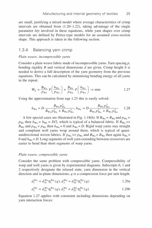
1.3.4 Balancing yarn crimp
Plain weave, incompressible yarns
Consider a plain weave fabric made of incompressible yarns. Yarn spacing p,bending rigidity B and vertical dimensions d are given. Crimp height h isneeded to derive a full description of the yarn geometry from the previousequations. This can be calculated by minimising bending energy of all yarnsin the repeat:
WBp
Fhp
Bp
FhpS
ÊË
ˆ¯
ÊË
ˆ¯ Æ = + minWa
We
Wa
We
We
Wa
We
Wa1.27
Using the approximation from eqn 1.23 this is easily solved:
h DB p
B p B ph D
B p
B p B pWaWe We
3
Wa Wa3
We We3 We
Wa Wa3
Wa Wa3
We We3 =
+ , =
+ 1.28
A few special cases are illustrated in Fig. 1.18(b). If BWa = BWe and pWa =pWe then hWa = hWe = D/2, which is typical of a balanced fabric. If BWa >>BWe and pWa = pWe then hWa = 0 and hWe = D. Rigid warp yarns stay straightand compliant weft yarns wrap around them, which is typical of quasi-unidirectional woven fabrics. If pWa >> pWe and BWa = BWe then again hWa =0 and hWe = D. Long segments of weft yarn extending between crossovers areeasier to bend than short segments of warp yarns.
Plain weave, compressible yarns
Consider the same problem with compressible yarns. Compressibility ofwarp and weft yarns is given by experimental diagrams. Subscripts 0, 1 and2 respectively designate the relaxed state, yarn dimension in the verticaldirection and in-plane dimensions; q is a compression force per unit length.
d d q d d q1Wa
10Wa
1Wa
2Wa
20Wa
2Wa = ( ), = ( )h h 1.29a
d d q d d q1We
10We
1We
2We
20We
2We = ( ), = ( )h h 1.29b
Equation 1.27 applies with constraint including dimensions depending onyarn interaction forces:

Design and manufacture of textile composites26
h h dQ
dd
QdWa We 10
Wa1Wa
2Wa 10
We1We
2We + = + h h
ÊËÁ
ˆ¯
ÊËÁ
ˆ¯
1.30
where the transversal forces Q are calculated from eqn 1.21, giving:
QB
p hF
hp
Bp h
Fhp
= + Wa
We Wa
Wa
We
We
Wa We
We
Wa
ÊË
ˆ¯
ÊË
ˆ¯ 1.31
Equation 1.30 assumes that the zone over which Q acts has dimensionsequal to in-plane yarn dimensions; a better description of the yarn contactzone would improve the model. The non-linear system (eqn 1.29–1.31) canbe solved iteratively by setting:
p Wap We
dWe
d Wa
hWa
hWe (a)
(b)
d20 = 2.6 mm d10 = 0.24 mm
Beforecompression Compressed
in the fabricCompressibility of the yarns
1.21.1
10.90.80.70.6
h 1, h 2
0 5 10 15 20Q(cN/mm)
Compressible 428.7 0.47 0.4 36Solid 429.1 0.53 0.5 32
mg/m2
Thickness(mm)
c(%)
Fibre volumefraction,Vf (%)
(c)
1.18 Balance of crimp in plain weave: (a) scheme; (b) three specialcases; (c) change in yarn dimensions for typical fabric withcompressible yarns.

Manufacturing and internal geometry of textiles 27
d d d d d d d d h h1Wa
10Wa
2Wa
20Wa
1We
10We
2We
20We
We Wa = , = , = , = , =
= ( + )/21Wa
1Wed d 1.32
Transversal forces are computed from eqn 1.31, yarn dimensions are obtainedfrom eqn 1.29 and the minimum problem of eqn 1.27 is solved for hWa andhWe. Then convergence is checked by comparing with values from eqn 1.32and the above steps are repeated as necessary.
Figure 1.18(c) shows an example of changes in yarn dimensions for aglass plain weave with tow linear density of 600 tex, tow bending rigidity of0.44 N mm2 and ends/picks count 36/34 yarns/cm. The compression diagramin Fig. 1.18(c) was measured using the KES-F tester. Results show that theyarns are compressed considerably, changing the fabric thickness by 8%.
1.4 Braided fabrics
1.4.1 Parameters and manufacturing of a 2D braidedfabric
In braiding, three or more threads interlace with one another in a diagonalformation, producing flat, tubular or solid constructions. Such fabrics canoften be used directly as net-shape preforms for liquid moulding processessuch as resin transfer moulding (RTM). This section discusses 2D flat ortubular braids.
Braiding process
The principle of braiding is explained in Figs 1.19 and 1.20 for a maypolemachine. Carriers move spools in opposite directions along a circular path.Yarn ends are fixed on a mandrel and interlace as shown in Fig. 1.19. Interlacedyarns move through the convergence zone of the machine, towards the mandrelwhich takes the fabric up the loom. The yarns follow helical paths on themandrel and interlace each time spools meet. Producing a thin, tight braidedlace or a circular tube does not require a mandrel. On the other hand, 2Dbraids produced on shaped mandrels can be used as reinforcements forcomposite parts. Braiding over shaped mandrels allows the introduction ofcurvature, section changes, holes or inserts in the reinforcement withoutneed to cut the yarns, as shown in the photograph in Fig. 1.19.
In the process described above spools must travel to and from the innerand outer sides of the circular path to create interlacing. Fig. 1.20 shows thenecessary spool motions for a part of the path. Carriers with odd and evennumbers move from left to right (clockwise) and from right to left (counter-clockwise) respectively. The notched discs are located on the circumference

Design and manufacture of textile composites28
of the machine, spool carrier axles are located in these notches and adjacentdisks rotate in opposite directions. Consider carrier 1; once taken by a diskto a position where notches superpose with those of the neighbouring diskthe carrier is transferred to that disk by centrifugal force and a rotating guide.Because of the difference in rotation directions, spool 1 is taken toward the
V (take up) Mandrel
Fell point
Convergence zone
Spool plane
+ w– w
Carrier with spool
CarriersConvergence
zone
Mandrel
(a)
(b)
1.19 Scheme and photograph of a maypole braider: diagonalinterlacing of the yarns, where only two carriers are shown. Insets:non-axisymmetric mandrel and braided products with holes andinserts.

Manufacturing and internal geometry of textiles 29
outside of the machine by the second disk. The same happens to its counterpart2 carried by the notched disks in the opposite direction. Hence carriers 1 and2 cross each other and change sides, creating interlacing. Figure 1.21(a)shows carrier paths producing a tubular braid. If the sequence of disks isinterrupted, the carriers create a flat braid as shown in Fig. 1.21(b). In modernbraiders notched disks are replaced by horn gears and carrier feet are directedalong slots in a steel plate covering the gears.
Additional yarns extending along the braid axis can be incorporated,producing what are commonly described as triaxial braids. They do nottravel on carriers but are fed from stationary guides situated at the centres ofhorn gears, Fig. 1.21(c). Such inlays or warp yarns are supported by thebraided yarns and are almost devoid of crimp. They are common inreinforcements.
Braid patterns and braiding angle
Patterns created by braiding are similar to weaves and can be described inthese terms (Fig. 1.22). Braids are identified in the same way as twills, byfloats lengths for the two interlacing yarn systems. Three patterns have specialnames: diamond (1/1), regular or plain (2/2) and hercules (3/3) braids. Aplain weave and a plain braid correspond to different patterns.
1
2
3
4
52
1 4 3
2
5
4
1
25 4 1 6
1.20 Horn gears and movements of the yarn carriers.

Design and manufacture of textile composites30
1.21 Carrier paths and braided patterns: (a) circular braid; (b) flatbraid; (c) braid with inlays (triaxial braid).
(a)
(b)
(c)

Manufacturing and internal geometry of textiles 31
1.22 Geometry of a braid unit cell: (a) dimensions of the unit cell;(b) geometry of crimp; (c) yarn crimp in a braid with inlays (darkeryarns).
d
p
s
a
I
(a)
(b)
(c)
h z(x ¢)
d ¢
x ¢p
z

Design and manufacture of textile composites32
The repeat of a braid is defined as the number of intersections required fora yarn to leave at a given point and to return to the equivalent position furtheralong the braid (arrows, Fig. 1.21). This measure is called plait, stitch or pickand equals the total number of yarns in a flat braid or half their number intubular braids. The definition differs from that of repeat in weaves; to avoidconfusion the term unit cell is used to identify the basic repetitive unit of apattern. The most important parameter of a braid is the braiding angle betweeninterlaced yarns (Fig. 1.22), calculated from the machine speed and mandreldiameter Dm:
a p = 2 arctan mD n
v1.33
where n and v are the rotational speed (s–1) and take-off speed. The angledepends on the mandrel diameter; if a complex mandrel is used the take-upspeed must be constantly adjusted to achieve a uniform angle. By varyingthe take-up speed variable angles can be induced, allowing stiffness variationsfor the composite part. The practical range of braiding angles is between 20∞and 160∞.
Equation 1.33 implies that the mandrel is circular (or at least axisymmetric),but as shown in Fig. 1.19 this is not a requirement for the process. Anaverage braid angle for a non-axisymmetric mandrel can be obtained byreplacing the term pDm in eqn 1.33 with the local perimeter of the mandrel.However, it has been observed that the braid angle changes significantlywith position around any section of a complex mandrel. Models have beenproposed recently to predict this behaviour11,12.
A braider can be set vertically or horizontally. The former is common forthe production of lace or general tubular braids, and the latter for braidingover long mandrels. Typical carrier numbers are up to 144. Rotation andtake-up speeds can reach 70 rpm (depending on carrier numbers) and 100 m/min respectively. Productivity as mass of fabric per unit time can be estimatedby the equation:
A TvN D TNn =
cos2
= 2
sin 2
m
ap
a 1.34
where T and N are the yarn linear density and number of carriers. Theproductivity can reach several hundreds of kilograms per hour; braiding ismore productive than weaving by an order of magnitude.
1.4.2 Internal geometry of 2D braids
The internal geometry of braids is governed by the same phenomenonmentioned for woven fabrics namely yarn crimp. The non-orthogonal interlacingof the yarns results in certain peculiarities. Consider a braided unit cell. Let

Manufacturing and internal geometry of textiles 33
n be a float in the braid pattern identified as n/n; n = 2 in Fig. 1.22. Unit celldimensions are given by the braiding angle, stitch length per unit cell s andline length per unit cell l:
l s = tan 2a 1.35
The shape of yarn centrelines can be modelled in a similar way as for wovenfabrics (Fig. 1.22b). On a section of the fabric including the centre of a yarn(axis x¢), spacing p and dimensions d¢ of support cross-sections are given by:
p s
n
l
nd d =
4 sin 2
= 4 cos
2
, = sin
2a a a¢ 1.36
where d is the yarn width. A function z(x¢) is constructed for a given crimpheight h using an elastica or Peirce-type model and crimp balance is computedusing the algorithm previously formulated. Observation of triaxial braidsreveals mostly straight and crimp-free inlays extending along the machinedirection. This is expected for balanced braids, while unbalanced braids arequite rare in practice. The presence of inlays changes the crimp height ofinterlacing yarns but the algorithms for the calculation of the mid-line shapeand crimp balance remain unchanged, (Fig. 1.22c).
When the braided yarns are not perpendicular the yarn paths will betwisted, so that yarn cross-sections appear rotated. This also applies to wovenfabrics subjected to shear deformation (for example during fabric draping).
1.4.3 3D braided fabrics
3D braiding presents some similarities with 2D braiding. In 2D maypolebraiding only two sets of carriers rotate around the braiding axis in oppositedirections, creating a single textile layer. In contrast, 3D braids can be regardedas multiple layers of interlaced yarns which are connected more or lessextensively by individual yarns extending through the thickness. It is possibleto braid preforms where the level of interlacing between different layers issuch that it becomes impossible to discern the distinct layers in the finalpreform. Carrier paths may be defined over concentric circles or Cartesianarrays, which are square or rectangular.
Two examples of 3D braiding processes are described by Byun and Chou13,known as the four-step and two-step processes. The four-step process (Fig.1.23a) uses a framework of yarn carriers in a rectangular or circular array. Asthe name suggests, the process consists of four steps, each involving alternatemovements of the rows and columns of yarn carriers. Between cycles theyarns are ‘beaten up’ into the structure and the braid is hauled off by onepitch length. The two-step process (Fig. 1.23b) involves a large number ofaxial yarns arranged in the required preform geometry, with a smaller number

Design and manufacture of textile composites34
of yarn carriers arranged around them. The carriers are moved through thearray of axial yarns in two alternate directions.
Such processes can be used to produce preforms featuring yarns thatextend along many directions. Yarn directions are not limited to a plane, andthis constitutes the main advantage of the process. However, any increase inout-of-plane properties is achieved at the expense of in-plane properties. 3Dbraids generally feature axial yarns. Preforms of various shapes can beproduced, for composite parts of which the geometry is very different to theshells associated to parts based on 2D textiles such as weaves or non-crimpfabrics. Such applications are still relatively rare; rocket engines constitute aclassic example while biomedical engineering is one area of emergence.
1.23 Schematic illustration of the (a) four-step and (b) two-step 3Dbraiding processes.
Braidedpreform
Braidingdirection
Yarn carrier
Machine bed
Step oneStep two
Step threeStep four
(a)
Steptwo
Stepone
Braider yarn Axial yarn
(b)

Manufacturing and internal geometry of textiles 35
1.5 Multiaxial multiply non-crimp fabrics
The above textile reinforcements offer economical advantages while beingeasier to process than prepregs. However, compromises are made on theperformance of the composite because of crimp that causes fibre misalignments.Non-crimp fabrics combine unidirectional crimp-free fibre layers by assemblingthem together by stitching – sewing or knitting – and/or bonding by chemicalagents.
1.5.1 Terminology and classification
European standard EN 13473 defines a multiaxial multiply fabric as
A textile structure constructed out of one or more laid parallel non-crimpednot-woven thread plies with the possibility of different orientations, differentthread densities of single thread plies and possible integration of fibrefleeces, films, foams or other materials, fixed by loop systems or chemicalbinding systems. Threads can be oriented parallel or alternating crosswise.These products can be made on machines with insertion devices (parallel-weft or cross-weft) and warp knitting machines or chemical bindingsystems.
The definition stresses that fibrous plies are laid up with threads. Stitchingthe plies together by warp-knitting can be achieved in such a way that thestitches pierce the plies between the laid yarns, resulting in an open preformarchitecture; Fig. 1.24a. On the other hand wide threads (flat tows) laid closetogether form continuous fibrous plies bound by warp-knitting with piercingsites positioned according to the needle spacing, without any connection totow positioning. Needles pierce the fibrous plies and distort them locally;Fig. 1.24b. Such a preform construction is close to ideal unidirectionaluniform plies. The latter case is the most common, and is the subject of thissection.
A fabric is characterised by the nature of the fibres (E/G/C/A glass, carbonor aramid), surface density of each ply (g/m2), fibre direction in each plygiven as an angle with respect to the machine direction in the range [–90∞,90∞], type of binding agent, nature of the binding agent (polyamide/poly(ethylene)/poly(ether sulphone)/poly(ethylene terephthalate/polypropylene;PA/PE/PES/PET/PP, chemical binder) and surface density of the bindingagent. For example the designation stipulated by the standard for a 3-ply+45∞/–45∞/0∞ glass fabric stitched by a polyester yarn is:
[G, 235, +45∞ // G, 235, –45∞ // G, 425, 0∞][PES, 12, L]
with a total surface density of 907 g/m2. Ply weight depends on yarn weightand placement density. In general yarn weight is characterised by a number

Design and manufacture of textile composites36
of filaments ranging from 3K to 80K for carbon tows. Surface densitiesusually range from 100 g/m2 upwards. Higher yarn weights normally translateinto higher ply surface density values for a closely covered surface. Lowsurface density values may be reached with thick tows by spreading, using aspecial unit. Yarns with higher fibre count present the economical advantagesof cheaper raw material and faster production. Low ply surface weights aredesirable as lighter fabrics have better drapability. Current technology achieves150 g/m2 with 12K yarns in the weft or 24K in 0∞ layers.
1.5.2 Manufacturing
Producing a multiaxial multiply fabric involves laying plies or weft insertion,and stitching or knitting them together. Hence the machine has two mainparts, a weft insertion device and a knitting unit.
(a)
(b)
1.24 Multiaxial multiply warp knitted fabrics: (a) open structure, withstitching sites in between the tows; (b) continuous plies, withstitching penetrating the tows forming ‘cracks’ in the plies.

Manufacturing and internal geometry of textiles 37
Weft insertion
Weft insertion carriages travelling across the machine lay several towssimultaneously at a desired angle across the fabric. The tows are fixed to theneedles of the moving chains. The length of the weft insertion part of atypical machine is about 10 m and allows up to three layers with angles from20∞ to 90∞ or –20∞ to –90∞. The speeds of weft insertion carriages dictate thefibre angles. Measurements show that the orientation of oblique fibres candeviate from the prescribed value by several degrees.
Weft inserted tows together with optional 0∞ plies are stitched by a warp-knitting device. A powder binder (e.g. epoxy) can be added beforehand tofacilitate composite processing. A foil or non-woven ply may be added belowthe plies. A warp-knitting device as described below stitches the plies by anaction of needles, which are collected in a needle bed and move upwards,piercing the plies.
Walking needle
Stitching of ply construction by warp-knitting is optimised to decreasemisalignment and disturbance of the weft yarns by the knitting needles. Inolder knitting units needles move in one direction only, standing at a certainangle to the plies. The needles move linearly upwards to catch the warpknitting yarn and then down to pull the yarn through the ply, building astitching mesh. Plies move constantly forward. The relative movement ofplies and needles in the horizontal direction causes misalignment duringpenetration, the extent of which depends on the stitching length and otherparameters. This limitation was reduced drastically by the development ofthe walking needle device, introducing a new needle movement where theneedle is placed at 90∞ to the textile and moves in the vertical direction aswell as in the direction of ply movement during penetration. The relativehorizontal motion between the textile and needle is minimal. The needlehead is designed to penetrate the ply construction by pushing away thefilaments of reinforcing yarns, minimising the damage.
Warp knitting
The principle of warp knitting is illustrated in Fig. 1.25. An actual warpknitted fabric or a knitted web, whereby warp knitting is used to stitchunidirectional fibrous plies, is an assembly of loops formed by the interactionof needles and guides. Yarns are fed through all guides and all needles arefixed on a needle bar, moving simultaneously and forming a loop aroundevery needle in every cycle.
Consider a warp yarn about to be looped, going thorough the guide at thebeginning of the knitting cycle (Fig. 1.25a). Knitting needles are in their

Design and manufacture of textile composites38
upper position. Loops forming the edge of the fabric are on the stems of theneedles. The guide carries the new yarn around a needle, forming a new loop(Fig. 1.25b,c). The needle moves down, connecting the new loop with theold one sitting on its stem (Fig. 1.25d,e); in the case of ply stitching the loopis pulled through the plies. The textile is pulled and a new cycle starts. Theknitting action creates loop connections in the machine (course) direction.Movements of the guides across the needle bed create connections in thecross (wale) direction, forming a warp-knit pattern; Fig. 1.26. The positionsof the gaps between the needles, where guides pass in subsequent knittingcycles, can be used to code the pattern by the so-called Leicester notation.Consider a diagram of the guides’ movement, called a lapping diagram (Fig.1.26). Rows of dots represent needle positions in plane view. The numberingof needles assumes that the pattern mechanism is on the right side. As theguides position themselves in the spaces between needles, the positions
1.25 Principle of warp knitting, showing interaction of the knittingneedles and guides.
Guide New yarn
D
Needles(a) (b)
(c) (d)
(e) (f)
New loop is formed Guidemoves to
a newneedle

Manufacturing and internal geometry of textiles 39
1.26 Warp-knit pattern formation and coding.
Gapidentifiers
4
3
2
1
Basicknittingsequences:
{3, 2}{4, 3}{1, 2}
Loops seen on theback of the fabric
Pattern seen onthe face of the
fabric

Design and manufacture of textile composites40
between vertical columns of dots represent lateral shifts of the guides. Thepattern is a sequence of these numbers:
s1–S1/s2–S2/ … / sN–SN 1.37
where si and Si are the positions of the guide forming the ith loop and N isthe number of knitting cycles in the pattern. Positions si and Si refer to gapsbetween needles where the elementary movement of guides start. A pair si–Si represents an overlap motion (guides move behind needles) while Si/si+1 isan underlap motion (guides move in front of needles). The following considerpatterns where overlaps extend by one needle only, i.e. Ási–Si Á= 1.
When fibrous plies are stitched, the pattern is seen on the face of thefabric (Fig. 1.26). These yarns are laid on the face of the fabric by the guides.On the back of the fabric chains of loops are seen, extending in the machinedirection. These loops are formed on separate needles and interconnect throughthe knitting action of the needles.
1.5.3 Internal geometry
Positions of the stitching sites
A stitching yarn pierces the fibrous plies at positions defined by the needlespacing in the needle bed (spacing in cross direction A) and by the speed ofthe material feeding in the knitting device (spacing in machine direction B).The value of A is also expressed by the machine gauge, a number of needlesper inch. In a warp-knitted fabric devoid of fibrous plies, yarn tension leadsto significant deviations of the actual loop spacing in the relaxed fabric. Inthe case of multiaxial multiply fabrics the stitching yarn is fixed by thefibrous plies, resulting in fairly regular spacing. Figure 1.27 gives an exampleof spacing variability for such a fabric. Deviations in the positions of stitchinglead to deviations of the loops from the ideal machine direction; the deviationcan be as high as 15∞.
Geometry of the stitching loop
The loop geometry can be assumed using a geometric approach or describedusing a mechanical approach where the shape is calculated from equilibriumequations applied to the looped yarns. The latter approach is unsuitable hereas loop positions are set by the plies, and large fluctuations of loop shapesare observed in practice. Hence the geometric approach is considered moreappropriate.
Stitching yarns normally have a low linear density of around 10 tex withtyically 15 filaments, and low twist (<100 m–1). They are easily compressible,which explains the large observed variations of their dimensions. Stitch yarn

Manufacturing and internal geometry of textiles 41
1.27 Spacing of the stitching loops for a carbon 0/–45/50 fabric:(a) definition of A and B and (b) measured values for adjacent wales.
(a)
A (
mm
)
6.00
5.00
4.00
3.00
2.00
1.00
0.001 2 3 4 5 6 7 8 9 10 11
Course no.
B (
mm
)
3.50
3.00
2.50
2.00
1.50
1.00
0.50
0.001 2 3 4 5 6 7 8 9 10
Course no.(b)

Design and manufacture of textile composites42
shapes are observed to vary within the repeating pattern, with cross-sectionsranging from circular to flattened (elliptical) and with varying dimensions14.
The geometry of the yarn centreline is defined by identifying a set ofanchor points A–M along the loop and approximating the centreline betweenthe anchor points by straight lines or circular arcs. In Fig. 1.28 h is the totalthickness of the plies; arcs AB, CD, FE, GH, IJ and KL have constant radiiand diameter d0. The loop width w depends on knitting tension. Considerabletension produces narrow loops with w ª 3d0; lesser tension increases w to 4to 5 times d0.
Interactions of the stitching with fibrous plies
Stitching causes deviations to fibre orientations. These deviations can resultin linear channels (Fig. 1.29a), or be localised near stitching sites as cracks(Fig. 1.29b). Localised cracks have a rhomboidal shape of width b andlength l. A channel is formed when localised cracks touch or overlap. Thedirection of cracks and channels corresponds to that of fibres in the ply. Thecracks/channels are also evident inside the fabric, where they provide routesfor resin flow. In a composite they create resin rich zones which can play animportant role in the initiation of damage.
Crack and channel dimensions feature much scatter (Fig. 1.29c). Table1.2 shows measured crack and channel dimensions for various fabrics. Crackwidths are approximately proportional to the thickness of the stitch yarn, sothat an empirical coefficient k can be used to calculate b = kd0, where d0 isthe compacted stitch diameter. Fibres in a powdered fabric are more difficultto displace, explaining the low values of k and l/b for the latter fabric. In non-powdered fabrics channels are wider than cracks, with rough k averages of 4(cracks) and 7 (channels) and l/w values for cracks of about 20. Dimensionsare also influenced by knitting tension.
When large channels extend along the machine direction, stitch yarn sectionson the fabric face or loops on the back can sink in the channels. Thisphenomenon plays a major role in nesting of non-crimp fabric layers inlaminates. When this sinking occurs the layers can come closer, closing anygap between them that might be introduced by stitched yarns laying on thesurface of the fabric. This is evidenced by compression curves of multiplelayers of fabric such as a biaxial ‘B’ –45∞/45∞ and quadriaxial ‘Q’ 0∞/–45∞/90∞/45∞; Fig. 1.30. In the former, stitch yarns extend across the fibre directionand cannot sink in cracks. The face of the latter textile has wide channelsinto which stitches sink deeply (Fig. 1.30a), allowing nesting. Hence thethickness per layer of the compressed fabric ‘Q’ decreases with an increasein number of layers while it stays constant for fabric ‘B’.

Manufacturing and internal geometry of textiles 43
zy
A B
G
HI
K
L MC
D
FE
x
y
I
d0 H
d0
G
d1m
inJ
KL
ME
xF
y
A
B
AJ
IG
BF
d0
wE
x
D
Cd
2max
LK
J
1.28
Geo
met
ry o
f th
e st
itch
ing
lo
op
s, s
ho
win
g p
osi
tio
ns
of
anch
or
po
ints
.
h

Design and manufacture of textile composites44
0 0.5 1.0 1.5b (mm)
Freq
uen
cy
0.30
0.25
0.20
0.15
0.10
0.05
0
0.3 0.4 0.5 0.6 0.7 0.8 0.9 1b (mm)
(c)
Freq
uen
cy
0.30
0.25
0.20
0.15
0.10
0.05
0
(a) (b)
1.29 Channels and cracks in the fibrous layers: (a) channels in a 0∞(face) ply; (b) crack in a 45∞ (back) ply; (c) distribution of channel/crack widths.

Manufacturing and internal geometry of textiles 45
Tab
le 1
.2
Dim
ensi
on
s o
f ch
ann
els
and
cra
cks
in m
ult
iaxi
al m
ult
iply
car
bo
n f
abri
cs
Fab
ric
Sti
tch
ing
Cra
ck/c
han
nel
w (
mm
)l
(mm
)k
l / w
Mat
eria
l, lin
ear
d0
(mm
)d
ensi
ty
–45/
–45,
12K
PE
S,
7.6
tex
0.08
8Fa
ce c
rack
s0.
276
5.05
3.13
18.3
Bac
k cr
acks
0.43
47.
155.
3916
.5
0/90
, 24
KP
ES
, 7.
6 te
x0.
088
Face
ch
ann
els
0.62
n/a
7.04
n/a
Bac
k ch
ann
els
0.36
n/a
4.09
n/a
0/–4
5/90
/45
PE
S,
7.6
tex
0.08
8Fa
ce c
han
nel
s0.
658
n/a
7.47
n/a
Bac
k cr
acks
0.48
37.
285.
4815
.0
45/–
45,
12K
PE
S,
6 te
x0.
071
Face
cra
cks
0.28
7.43
3.94
26.5
Bac
k cr
acks
0.27
7.85
3.80
29.1
0/90
, 12
K,
po
wd
ered
PA,
10 t
ex0.
107
Face
ch
ann
els
0.18
n/a
1.68
n/a
Bac
k cr
acks
0.53
3.46
4.95
6.53

Design and manufacture of textile composites46
(a)
1 layer
4 layers
2 layers
Th
ickn
ess
per
lay
er (
mm
)
1.3
1.2
1.1
1.0
0.9
0.8
0.7
0.60 1 2 3 4 p(kPa)
(b)
Th
ickn
ess
per
lay
er (
mm
)
1.4
1.3
1.2
1.1
1.0
0.9
1 layer
4 layers
2 layers
0 1 2 3 4 p(kPa)(c)
1.30 Sinking of the stitching in channels in the fibrous plies: (a) fabric‘Q’ (see text), photo and schematic, and compression curves for (b)biaxial fabric ‘B’ and (c) quadriaxial fabric ‘Q’.

Manufacturing and internal geometry of textiles 47
1.6 Modelling of internal geometry of textile
preforms
Textiles are hierarchically structured fibrous materials. As discussed in theclassic paper by Hearle et al.15 this description of the nature of textilesallows efficient construction of mathematical models for the geometry andthe mechanical behaviour of textile structures. In spite of the generallyrecognised usefulness of this approach, it has not been used to its full strengthfor the creation of textile structure models. During the 1930s the first seriousmechanical treatments of the structure of textile materials were published byPeirce10, Pozdnyakov16 and Novikov17. Since then, numerous publicationshave been proposed on the mechanical behaviour of textiles, culminating ina comprehensive treatment on Mechanics of Flexible Fibre Assemblies in198018. In the following years the ideas and approaches outlined in this bookwere pursued further. Textile mechanics at the outset of the 21st centuryincludes models of the internal geometry of textile structures such ascontinuous-filament and staple yarns, random fibre mats, woven and knittedfabrics. The hierarchical description of textile structures is implementedusing the minimum energy principle as introduced by Hearle and Shanahan19
and de Jong and Postle20. This allows the decomposition of a structure intoa set of structural elements, leading to models that are physically sound andcomputationally feasible. It should be noted that the principle of minimumenergy is heuristic when applied to non-conservative mechanical systemssuch as textiles.
Following the hierarchical approach one can consider a description of theinternal geometry of a fabric on two different levels: the yarn paths modedescribing the spatial configuration of yarns and the fibre distribution modedescribing spatial distribution properties of the fibrous assembly. In the formercase the fabric is regarded as an agglomeration of yarns – slender curvedbodies. Their spatial positions are defined by description of yarn midlinesand cross-section at each point of the midlines. The internal fibrous structureof the yarns is not considered. In the latter case the fibrous structure of yarnsshould be defined. The definition of the spatial positions of yarns stateswhether any point in the unit cell lies inside a yarn or not; if so, parametersof the fibrous assembly at this point are determined. The yarn path mode issufficient for the calculation of simpler data related to the internal geometry,such as surface density, fabric thickness and local inter-yarn porosity. Thefibre distribution mode is needed when detailed information on the fibrousstructure is required.
1.6.1 Yarn path mode
Figure 1.31 illustrates the description of yarn spatial configuration. The mid-line of the yarn shown in Fig. 1.31b is given by the spatial positions of the
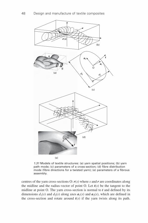
Design and manufacture of textile composites48
centres of the yarn cross-sections O: r(s) where s and r are coordinates alongthe midline and the radius-vector of point O. Let t(s) be the tangent to themidline at point O. The yarn cross-section is normal to t and defined by itsdimensions d1(s) and d2(s) along axes a1(s) and a2(s), which are defined inthe cross-section and rotate around t(s) if the yarn twists along its path.
O
r(s)
(b)
(a)
A
B
ta2
a1
O
d2 d1
(c)
(d)
PVf
f
(e)
1.31 Models of textile structures: (a) yarn spatial positions; (b) yarnpath mode; (c) parameters of a cross-section; (d) fibre distributionmode (fibre directions for a twisted yarn); (e) parameters of a fibrousassembly.

Manufacturing and internal geometry of textiles 49
Because of this rotation the system [a1a2t] may differ from coordinate systemalong the path.
A definition of the spatial position of a yarn with a given cross-sectionshape therefore consists of the five functions r(s), a1(s), a2(s), d1(s), d2(s).Models defining these functions for different textile structures were describedin previous sections. Two approaches are possible for definition of the midlinepath r(s): a simpler geometric and a more complex mechanical one.
Geometric approach
In the geometric approach, midline anchor points are defined from topologicalinformation for the textile structure. These points can be located at yarncontacts or crossovers for some textiles, as the distance between contactingyarns is known from cross-section dimensions. For more complex textiles inmay be necessary to introduce additional points to represent some curvatures.Yarn midlines are represented by smooth lines going through these points;typically Bézier curves are used21–23.
The main advantage of the geometric approach is that it can represent anytextile structure under one single format while producing simple and portabledefinitions. As a result, downstream models of the physical properties oftextiles and their composites can be used with these geometric definitions,regardless of the textile manufacturing process. Furthermore, the format isequally well suited to simpler closed-form physical property models as it isto more computationally intensive ones. The philosophy behind the geometricapproach consists in creating geometric models that are ensured to beappropriate, devoid of interference for example, with the view of refining theassumed initial geometry through mechanical methods, and this for anytextile and manufacturing processes. Figure 1.32 shows diverse examples,with anchor points forming 3D linear segments represented as vectors on theleft and the resulting geometric models on the right. Any interferences resultingfrom user input were corrected by a geometric algorithm where sections aremodified arbitrarily and yarn Vf remains constant. Another major advantageis that it allows explicit consideration of important practical phenomenasuch as the statistical variation of dimensions inherent within actual textiles.
Although the geometric approach method offers the advantages of simplicity,speed and certainty over aspects such as interference, the models that itproduces clearly depend on user input. The anchor points are predefined andassumptions are made about yarn interaction or crimp height, for example.Symmetry considerations can assist but only to a certain extent, and in itsbasic form predictive geometry determination is not possible. For an accuratedescription, dimensions must be measured from real fabrics.

Design and manufacture of textile composites50
Mechanical approach
A mechanical approach to the modelling of yarn paths requires a mathematicaldescription of the interaction of contacting yarns. In relaxed fabrics thisinvolves bending and compression of yarns; twisting may also be present.Therefore, it also requires appropriate experimental data for the yarns inthese deformation modes. If this is available, the model must account forcontacts between interacting yarns and describe the equilibrium of the finalconfiguration. The minimum energy principle is normally used for thisdescription. Examples of such models were shown above for weaves and braids.
1.32 Geometric approach to textile modelling for a range of textiles,showing vectorial description of yarn paths (left) and resulting textilemodels (right).

Manufacturing and internal geometry of textiles 51
Computational efficiency is critical in the mechanical approach and thereforethe definition of fabric geometry should use the principle of hierarchy andstructure decomposition. The repeat is a natural structural unit for fabricsand contains a number of yarns {Y} that contact others. The contact regionsoccupy certain zones on the yarns. Characteristic points provide naturalboundaries for structural elements of the repeat (Fig. 1.31a). In a wovenfabric the structural elements consist of intervals of warp and weft yarnslocated between subsequent crossovers, where characteristic points are located.
A yarn Y consists of a set of structural elements {e}Y, each characterisedby the coordinates of its end points AYe and BYe, the dimensions of the contactregions near the end-points, and the forces acting on the contact regions. Theexact shape and dimensions of the contact regions on a structural elementand the forces acting on them are determined by yarn interactions in thestructure.
The basic assumption of the decomposition routine is that the spatialpositions of the end-points of structural elements play a central role incalculating the geometry of that element. Supposing that the end positions ofthe structural elements for all yarns in a repeat are known and fixed, contactregions develop near the end-points due to yarn interactions, and internalforces arise in the contact zones. Geometric constraints imposed on thestructure by the end-point positions determine the local deformations ofyarns at contact regions and the shape and dimensions of these regions,which in turn determine the contact forces.
In general cases a set of parameters q1, q2, q3, … are designated thatdetermine the complex mechanical behaviour of structural elements. Relatingto the assumption formulated in previous paragraphs, these parameters consistof the positions of end-points of the structural elements, {qi} = {A, B}.
Consider now the problem of computing the spatial position of yarns inthe fabric repeat space. Let rY(s) be the parametric representation of thecentreline of yarn Y. According to the minimum energy principle the set ofrY(s) for all yarns in the fabric repeat should satisfy:
S( )
[ ( )] minY YW sr Æ 1.38
If rY(s) is split into separate functions for each structural element e on yarnY this takes the form:
S S( ) ( )
[ ( )] minY e
YeW sr Æ 1.39
which can be recast as:
S S( ) ( )
1 2 3 [ ( ; , , )] minY e
YeW s q q qr º Æ 1.40

Design and manufacture of textile composites52
This global minimisation problem can be reformulated as a series ofminimisation problems for structural elements:
min [ ( ; , , )]( ) ( ) ( )
1 2 3rr
s Y eYeW s q q qS S º
= min min { [ ( | , , )]}1 2 3, , ( ) ( ) ( ) 1 2 3q q q Y e s YeW s q q q
ººS S
rr 1.41
Each minimisation problem should be solved with parameters {qi} fixed,yielding the solution:
min( )r s
{W[r(s | q1, q2, q3 …)]} fi r(s | q1, q2, q3…) 1.42
which is used to calculate the energy of the structural element:
r(s | q1, q2, q3 …) fi W(q1, q2, q3 …) 1.43
The function W, which depends only on parameters of the structural element,is termed the characteristic function of the structural element. The minimisationproblem (1.40), which has the functions rY(s) as arguments, is reduced to thefollowing minimisation problem:
S SY e
YeW q q q ( , , ) min1 2 3º Æ 1.44
where the arguments are a set of scalar parameters {qi}. This leads to asystem of non-linear algebraic equations instead of differential or integralequations, which would result from eqn 1.38. A practical application of thisappears in section 1.3.3 for a simple weave. Note that the energy functionsinvolved in eqn 1.44 may represent bending, compression and torsion andaccounting for non-linearity.
Mechanical models aim to be predictive and to determine the structure offabrics from independent measurements of yarn properties. In some casesthis cannot be achieved as yarns undergo mechanical loading during fabricmanufacture and the resulting deformations are not relaxed, leading todeviations between reality and analysis based on equilibrium in the relaxedstate. This is especially true for cases when manufacturing tensions are extreme,say for example in 3D weaving. For such cases one must rely on a geometricmodel coupled with physical measurements taken from the fabric.
Using yarn path mode
The yarn path mode (mesoscopic geometric model) is a necessary step inbuilding models at the microscopic scale (fibre distribution mode). Mesoscopicmodels also have inherent value: they define yarn volumes and thereforeinter-yarn porosity, as well as local fibre directions of yarns. Information on

Manufacturing and internal geometry of textiles 53
the local direction of the yarns is essential for most predictive models of thephysical properties of textiles, say for example in micro-mechanical modelsof composites to calculate the homogenised stiffness matrix of the unit cell,or in permeability models for composites processing. One approach to theformer consists in defining ellipsoidal inclusions with stiffness propertiesequivalent to those of elements of the impregnated yarn, and then using thesolution of Eshelby for homogenising the stiffness of agglomerated inclusions24.Both approaches rely on a representation of the local, microscopic fibrousstructure as a unidirectional array of fibres, the equivalent stiffness of whichis obtained from empirical formulae25 or finite element analysis results26.These issues are discussed further in Chapter 8.
The second use of the yarn path mode is related to numerical modelling.The geometry of yarn volumes can be easily transferred to mesh generators;(Fig. 1.33). Yarn segments can be assembled into solid models of fabrics andmeshed. The geometry of the empty volumes extending between the yarns isfar more intricate; this must also be meshed for problems of flow and heattransfer through textiles and for all problems related to textile composites.Although commercial solid modellers can sometimes process this, good resultsoften require very high mesh densities. Other solution techniques that do notuse conformal meshing, or that simplify the problem, constitute importanttopics towards the routine use of such tools as a support to industrial designof textile applications. Figure 1.34 shows a 2.5D mesh used for calculatingin-plane permeability tensors of textile reinforcements based on a simplified,efficient technique27.
1.6.2 Fibre distribution mode
Yarn path mode geometric modelling describes yarn volumes but says nothingabout the fibrous structure of yarns, unit cells or fabrics. The fibre distributionmode provides such information. Consider a point P (Fig. 1.31e) and afibrous assembly in the vicinity of this point. The assembly can be characterisedby different parameters including physical and mechanical properties of thefibres near point P (which may vary throughout the fabric), fibre volumefraction Vf and direction f. Length distribution of fibres near the point, averagecurvature and other parameters can be specified if the point is in a yarn. Afibre distribution mode model should provide such information for any point P.
Using fibre distribution mode
The ability to query the fibrous structure near arbitrary points can be used inmany applications dealing with mesh representations of heterogeneous media.In finite element representations of fabrics the fibre distribution mode is usedto determine mechanical properties for each element. Figure 1.33(c) illustrates
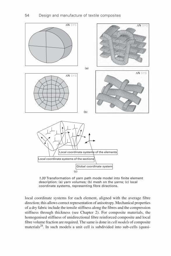
Design and manufacture of textile composites54
local coordinate systems for each element, aligned with the average fibredirection; this allows correct representation of anisotropy. Mechanical propertiesof a dry fabric include the tensile stiffness along the fibres and the compressionstiffness through thickness (see Chapter 2). For composite materials, thehomogenised stiffness of unidirectional fibre reinforced composite and localfibre volume fraction are required. The same is done in cell models of compositematerials28. In such models a unit cell is subdivided into sub-cells (quasi-
1.33 Transformation of yarn path mode model into finite elementdescription: (a) yarn volumes; (b) mesh on the yarns; (c) localcoordinate systems, representing fibre directions.
LN SYSLN SYS
LN SYSLN SYS
(a)
(b)
Local coordinate systems of the elements
Local coordinate systems of the sections
Global coordinate system
(c)

Manufacturing and internal geometry of textiles 55
finite elements), the effective stiffness of which is calculated from averageproperties of the local fibrous assembly or matrix.
In models of flow through the reinforcement, a regular mesh or lattice isdefined in the unit cell. Nodes of the lattice can lie outside or inside theyarns. In the former case the Navier–Stokes equation governs the fluid flownear the node. In the latter case the flow is described by the Brinkmannequation. The local permeability of the media is calculated using a unidirectionaldescription of the fibrous assembly near the node. These equations are solvedsimultaneously for all the nodes in the unit cell, using, for example, thelattice Boltzmann method29 or commercial software30.
1.6.3 Implementation of textile hierarchical model
Table 1.3 shows the hierarchy of structural elements in textile composites,and the modelling problems associated with each scale. Unnecessary mixtureof hierarchical levels should be avoided: yarn data should be used to predictbehaviour of fabrics as opposed to fibre data, and so forth. Each hierarchylevel is occupied by models which use data from that level and the next lowerto predict properties of the defined structure at the next upper level.
Object oriented programming provides a powerful tool for the constructionvirtual textiles. Associated data fields and methods are outlined in Table 1.4.The results of geometric modelling serve as crucial input to models ofcomposites processing and mechanical behaviour. The main advantage isthat local variations in textile geometry, and hence in physical properties,
1.34 Mesh representing local yarn and resin/free volume mid-planesfor a single crossover of a plain weave. Each element has anassociated thickness (free volumes) or permeability (yarn). Thismodel is used for the ‘streamsurface’ permeability predictionmethod27.

Design and manufacture of textile composites56
can be accounted for explicitly. A composite material, as the final product inthe sequence ‘fibre to yarn to textile to preform to composite’, is included inthe hierarchical description of the textile, taking full advantage of the versatilityof the approach.
Fabrics are usually assembled into laminates to form reinforcements withappropriate thickness. The layers of the laminate are not precisely positionedone against another, causing a geometric and mechanical phenomenon ofnesting. Nesting plays an important role in determining the physical propertiesof dry laminated reinforcements and composite parts. It causes statisticaldistribution of the laminate properties, both within one part and betweendifferent parts. A study of the nesting effect is therefore important for thecorrect representation of the internal geometry in predictive models ofprocessing and performance and for the assessment of the statisticalcharacteristics of properties, determining processing parameter windows andconfidence intervals for the performance indicators. Such an approach ispossible using a hierarchical model of the type described here31.
Table 1.3 Hierarchy of structure and models of a textile composite
Structure Elements Models
Yarn (tow) Fibres Fibre distribution in the yarn and itschange under load/strainMechanical properties of the yarn
Fabric (woven, Yarns Geometry of yarns in the fabric andknitted…) its change under load/strain
Mechanical behaviour of the fabricrepeat under complex loading
Composite unit cell Fabric Mechanical properties (stiffnessmatrix/non-linear law; strength)
Matrix Permeability tensor
Composite part (Deformed/ Behaviour under loadingdraped) unit Flow of the resincells Behaviour in the forming process

Manufacturing and internal geometry of textiles 57Ta
ble
1.4
Im
ple
men
tati
on
of
virt
ual
tex
tile
mo
del
via
OO
P a
pp
roac
h
Ob
ject
Dat
aM
eth
od
s
Gro
up
Fiel
ds
Fib
reG
ener
alLi
nea
r d
ensi
ty (
tex)
Dia
met
er (
mm
)D
ensi
ty (
g/c
m3 )
Mec
han
ics
Ela
stic
co
nst
ants
Ten
acit
y (M
Pa)
Ult
imat
e el
on
gat
ion
Yarn
Gen
eral
Yarn
typ
e: m
on
ofi
lam
ent,
Co
mp
ute
mas
s fo
r a
giv
en l
eng
thco
nti
nu
ou
s fi
lam
ent
or
spu
nLi
nea
r d
ensi
ty (
tex)
Geo
met
ry o
f th
eA
ssu
med
sh
ape:
elli
pti
cal/
Co
mp
ute
vo
lum
e o
f th
e g
iven
yar
ncr
oss
-sec
tio
nle
nti
cula
r/re
ctan
gu
lar
len
gth
Dim
ensi
on
s o
f cr
oss
-sec
tio
n i
nD
eter
min
e, w
het
her
th
e g
iven
po
int
free
sta
te d
01, d
02 (
mm
)( x
, y )
lie
s in
sid
e th
e ya
rnC
om
pre
ssio
nTy
pe
of
com
pre
ssio
n b
ehav
iou
r:C
om
pu
te c
om
pre
ssed
yar
nn
o c
om
pre
ssio
n,
spec
ifie
dd
imen
sio
ns
un
der
a g
iven
fo
rce
per
com
pre
ssio
n l
awu
nit
len
gth
Co
mp
ress
ion
co
effi
cien
t h 1
= d
1/d
10/
Co
mp
ute
co
mp
ress
ion
of
two
fun
ctio
n o
f co
mp
ress
ive
forc
e Q
inte
rsec
tin
g y
arn
s fo
r g
iven
no
rmal
per
un
it l
eng
thfo
rce
and
in
ters
ecti
on
an
gle
Flat
ten
ing
co
effi
cien
t h 2
= d
2/d
20/
fun
ctio
n o
f co
mp
ress
ive
forc
e Q
per
un
it l
eng
thB
end
ing
Ben
din
g c
urv
e ‘t
orq
ue–
curv
atu
re’
Co
mp
ute
ben
din
g r
igid
ity
valu
e B
(lin
ear
for
con
stan
t b
end
ing
for
a g
iven
cu
rvat
ure
rig
idit
y) M
( k)
(Co
ntd
)

Design and manufacture of textile composites58
Tab
le 1
.4 (
Co
nti
nu
ed)
Ob
ject
Dat
aM
eth
od
s
Gro
up
Fiel
ds
Fric
tio
nFr
icti
on
law
yar
n-y
arn
in
th
e fo
rmC
om
pu
te f
rict
ion
fo
rce
for
a g
iven
F =
fNn,
wh
ere
N i
s a
no
rmal
fo
rce
no
rmal
fo
rce
Yarn
wit
hIn
her
its
dat
a an
d m
eth
od
s o
f ya
rn.
Ad
ds
the
follo
win
g a
nd
rep
lace
s (b
old
) so
me
of
yarn
met
ho
ds
fib
re d
ata
Gen
eral
Twis
t (1
/m)
Co
mp
ute
th
e tw
ist
ang
leTw
ist
dir
ecti
on
(S
or
Z)
Co
mp
ute
lin
ear
den
sity
fro
m f
ibre
dat
aFi
bre
Fib
re d
ata
(fib
re o
bje
ct)
Co
mp
ute
fib
rou
s co
nte
nt
and
fib
reN
um
ber
of
fib
res
in c
ross
-sec
tio
nd
irec
tio
n i
n t
he
vici
nit
y o
f th
e g
iven
Fib
re d
istr
ibu
tio
n i
n t
he
yarn
po
int
( x,
y ).
Co
mp
ress
ion
Co
mp
ute
co
mp
ress
ed y
arn
dim
ensi
on
san
d f
ibre
dis
trib
uti
on
in
it
Ben
din
gC
om
pu
te b
end
ing
res
ista
nce
fro
mfi
bre
dat
a
Yarn
pat
hIm
ple
men
ts y
arn
pat
h m
od
eFi
bro
us
asse
mb
lyH
old
s a
refe
ren
ce t
o y
arn
wit
hfi
bre
dat
a o
bje
ctYa
rn p
ath
Arr
ay o
f d
escr
ipti
on
s o
f d
imen
sio
ns
Co
mp
ute
yar
n v
olu
me,
len
gth
an
dan
d o
rien
tati
on
of
yarn
cro
ss-s
ecti
on
sm
ass
Co
mp
ute
ave
rag
e fi
bre
vo
lum
e fr
acti
on
Fab
ric
Gen
eric
des
crip
tio
n o
f a
fab
ric
Fib
rou
s as
sem
bly
Arr
ay o
f ya
rn p
ath
ob
ject
sB
uild
th
e ya
rn d
escr
ipti
on
s (a
bst
ract
).C
om
pu
te o
vera
ll fa
bri
c p
aram
eter
s:d
imen
sio
ns
of
un
it c
ell,
area
ld
ensi
ty,
fib
re v
olu
me
frac
tio
nC
om
pu
te l
oca
l fi
bre
dat
a at
giv
en p
oin
t

Manufacturing and internal geometry of textiles 59
Tab
le 1
.4 (
Co
nti
nu
ed)
Ob
ject
Dat
aM
eth
od
s
Gro
up
Fiel
ds
Vis
ual
ise
the
fab
ric
Exp
ort
dat
a fo
r m
icro
-mec
han
ical
an
dp
erm
eab
ility
an
alys
is
Wo
ven
fab
ric
Inh
erit
s fr
om
fab
ric
ob
ject
. A
dd
s an
d r
epla
ces
(bo
ld)
the
follo
win
gTo
po
log
yW
eave
co
din
gYa
rns
Ref
eren
ces
to y
arn
wit
h f
ibre
dat
ao
bje
cts
for
all
yarn
s in
fab
ric
rep
eat
Sp
acin
gE
nd
s/p
icks
co
un
tFi
bro
us
asse
mb
lyB
uild
th
e ya
rn d
escr
ipti
on
s

Design and manufacture of textile composites60
References
1. Kurashiki T., Zako M. and Verpoest I., ‘Damage development of woven fabriccomposites considering an effect of mismatch of lay-up’, Proc. 10th European Conf.on Composite Materials, Brugge, June 2002 (CD edition).
2. Kawabata, S., The Standardisation and Analysis of Hand Evaluation, Osaka, TextileMachinery Society of Japan, 1975.
3. Hearle J.W.S., Grosberg P. and Baker S., Structural Mechanics of Fibres, Yarns andFabrics, New York, Wiley Interscience, 1969.
4. Abbot G.M., ‘Yarn-bending and the weighted-ring stiffness test’, J. Textile Institute,1983 74(5) 281–286.
5. Lomov S.V., Truevtzev A.V. and Cassidy C., ‘A predictive model for the fabric-to-yarn bending stiffness ratio of a plain-woven set fabric’, Textile Research J., 200070(12) 1088–1096.
6. Grishanov S.A., Lomov S.V., Harwood R.J., Cassidy T. and Farrer C., ‘The simulationof the geometry of two-component yarns. Part I. The mechanics of strand compression:simulating yarn cross-section shape’, J. Textile Institute, 1997 88 part 1(2) 118–131.
7. Harwood R.H., Grishanov S.A., Lomov S.V. and Cassidy T., ‘Modelling of two-component yarns. Part I: The compressibility of yarns’, J. Textile Institute, 1997 88Part 1 373–384.
8. Potluri P., Wilding M.A. and Memon A., ‘A novel stress-freezing technique forstudying the compressional behaviour of woven fabrics’, Textile Research J., 200272(12) 1073–1078.
9. Love A.E.H., A Treatise on the Mathematical Theory of Elasticity, New York, DoverPublications, 1944.
10. Peirce F.T., ‘The geometry of cloth structure’, J. Textile Institute, 1937 28(3) T45–T96.
11. Long A.C., ‘Process modelling for liquid moulding of braided preforms’, CompositesPart A, 2001 32(7) 941–953.
12. Kessels J.F.A. and Akkerman R., ‘Prediction of the yarn trajectories on complexbraided preforms’, Composites Part A, 2002 33(8) 1073–1081.
13. Byun J.H. and Chou T.W., ‘Process–microstructure relationships of 2-step and 4-step braided composites’, Composites Sci. Technol., 1996 56 235–251.
14. Lomov S.V., Belov E.B., Bischoff T., Ghosh S.B., Truong Chi T. and Verpoest I,‘Carbon composites based on multiaxial multiply stitched preforms. Part 1. Geometryof the preform’, Composites Part A, 2002 33(9) 1171–1183.
15. Hearle J.W.S., Konopasek M. and Newton A., ‘On some general features of a computer-based system for calculation of the mechanics of textile structure’, Textile ResearchJ, 1972 42(10) 613–626.
16. Pozdnyakov B.P., Fabric Resistance to Tension in Different Directions, Moscow-Leningrad, GIZLegProm., 1932, 70 (in Russian).
17. Novikov N.G., ‘A fabric structure and its design with the geometrical technique’,Textilnaya Promishlennost, 1946 6(2) 9–17 (in Russian).
18. Hearle J.W.S., Amirbayat J. and Twaites J.J. (editors), Mechanics of Flexible FibreAssemblies, Alphen aan den Rijn, Sijthoff and Nordhof, 1980.
19. Hearle J.W.S. and Shanahan W.J., ‘An energy method for calculations in fabricmechanics’, J Textile Institute, 1978 69(4) 81–110.
20. de Jong S. and Postle R., ‘A general energy analysis in fabric mechanics usingoptimal control theory’, Textile Research J., 1978 48(3) 127–135.

Manufacturing and internal geometry of textiles 61
21. Robitaille F., Clayton B.R., Long A.C., Souter B.J. and Rudd C.D., ‘Geometricmodelling of industrial preforms: woven and braided textiles’, Proc. Institution ofMechanical Engineers Part L, 1999 213 69–84.
22. Robitaille F., Clayton B.R., Long A.C., Souter B.J. and Rudd C.D., ‘Geometricmodelling of industrial preforms: warp-knitted textiles’, Proc. Institution of MechanicalEngineers Part L, 2000 214 71–90.
23. Goktepe O. and Harlock S.C., ‘Three-dimensional computer modelling of warpknitted structures’, Textile Research J, 2002 72(3) 266–272.
24. Huysmans G., Verpoest I. and Van Houtte P., ‘A poly-inclusion approach for theelastic modelling of knitted fabric composites’, Acta Materials, 1998 46(9) 3003–3013.
25. Chamis C.C., ‘Mechanics of composite materials: past, present and future’, J.Composites Technol. Res., 1989 11(1) 3–14.
26. Carvelli V. and Poggi C., ‘A homogenization procedure for the numerical analysis ofwoven fabric composites’, Composites Part A, 2001 32(10) 1425–1432.
27. Robitaille F., Long A.C. and Rudd C.D., ‘Geometric modelling of textiles for predictionof composite processing and performance characteristics’, Plastics Rubber andComposites, 2002 31(2) 66–75.
28. Vandeurzen P., Ivens J. and Verpoest I., ‘Micro-stress analysis of woven fabriccomposites by multilevel decomposition’, J. Composite Materials, 1998 32(7) 623–651.
29. Belov E.B., Lomov S.V., Verpoest I., Peters T., Roose D., Parnas R.S., Hoes K. andSol V., ‘Modelling of permeability of textile reinforcements: lattice Boltzmann method’,Composites Sci. Technol., 2004 64(7–8) 1069–1080.
30. Long A.C., Wong C.C., Sherburn M. and Robitaille F., ‘Modelling the effect of fibrearchitecture on permeability for multi-layer preforms’, Proc 25th SAMPE EuropeInt. Conf., Paris, March/April 2004, pp. 325–330.
31. Lomov S.V., Verpoest I., Peeters T., Roose D. and Zako M., ‘Nesting in textilelaminates: geometrical modelling of the laminate’, Composites Sci. Technol., 200363(7) 993–1007.

62
2.1 Introduction
This chapter describes the mechanical behaviour of textile reinforcements,with the primary aim of understanding their behaviour during forming andconsolidation processes. A number of deformation mechanisms are available.However, during typical composites manufacturing processes, it is generallyagreed that the most important of these are in-plane shear and tensile behaviourand through-thickness compaction. Of these mechanisms, the ability of fabricsto shear in-plane is their most important feature during forming, althoughgiven their low shear stiffness, in-plane tensile behaviour represents thelargest source of energy dissipation. Compaction behaviour defines the fibrevolume fraction that can be obtained after manufacturing. Other propertiessuch as fabric bending and ply/tool friction are not considered here, primarilybecause these have received relatively little attention elsewhere and littledata are available.
This chapter introduces a number of experimental methods for characterisingthe deformation of textiles. These methods have been developed within researchstudies, usually to obtain material data for manufacturing simulation (seeChapter 4). One important consideration here is that none of these tests isstandardised – and in fact nearly all published studies use slightly differenttest methods and specimen dimensions. This issue is being addressed atpresent as part of a round-robin exercise1. Several standard tests are used inthe wider textiles community (e.g. BS ISO 4606:1995, BS 3356:1990, BS3524-10:1987). Of particular relevance here is the ‘Kawabata EvaluationSystem for Fabrics (KES-F)’, a series of test methods and associated testingequipment for textile mechanical behaviour including tensile, shear, bending,compression and friction2. However, while this system has been used widelyfor clothing textiles, its application to reinforcement fabrics has been limited3.This is probably because KES-F provides single point data at relatively lowlevels of deformation, coupled with the limited availability of the (expensive)testing equipment.
2Mechanical analysis of textiles
A C L O N G, University of Nottingham, UK,P B O I S S E , INSA Lyon, France and
F R O B I T A I L L E , University of Ottawa, Canada

Mechanical analysis of textiles 63
As discussed in Chapter 1, the geometry of textile reinforcements can bedescribed at a number of length scales. Individual fibres represent themicroscopic scale, with large numbers of fibres (typically several thousand)making up the tow or yarn. The scale of the yarns and of the fabric repeatingunit cell is the mesoscopic scale. Finally, the fabric structure constitutes themacroscopic scale. The macroscopic mechanical behaviour of fabrics dependson phenomena at smaller scales, and in particular it is dependent on geometricand contact non-linearities. Such considerations will be used throughout thischapter to develop predictive models for textile mechanical behaviour.
2.2 In-plane shear
2.2.1 Characterisation techniques
As mentioned above, in-plane (or intra-ply) shear is generally considered tobe the primary deformation mechanism during forming of textile reinforcementsto three-dimensional geometries. Characterisation of this mechanism hastherefore received a great deal of attention. The objectives are usually twofold:to measure the non-linear mechanical response of the material during shear,and to characterise the limit of deformation. At the simplest level, mechanicalbehaviour is of interest for ranking of materials in terms of ease of forming.More recently such data have been required for mechanical forming simulationsoftware based on finite element analysis (see Chapter 4). Here shear forceshould be normalised by a representative length to eliminate sample sizeeffects. The limit of forming is often characterised by measurement of the‘locking angle’, which represents the maximum level of shear deformationthat can be achieved before fabric wrinkling occurs. In practice this limitvaries widely and is highly dependent on the test method employed. Theprimary use of locking angle data is to identify areas of wrinkling withinkinematic draping codes for fabric forming.
The majority of published studies have characterised resistance to intra-ply shear using two approaches (Fig. 2.1). Bias extension tests, involvinguniaxial extension of relatively wide samples in the bias direction, are favouredby a number of researchers4–6, as the testing procedure is relatively simple.However the deformation field within the sample is non-uniform, withmaximum shear observed in the central region and a combination of shearand inter-yarn slip observed adjacent to the clamped edges. In addition theshear angle cannot be obtained directly from the crosshead displacement, sothat the test must be monitored visually to measure deformation. Neverthelessthis test can provide a useful measure of the locking angle, which in this caserepresents the maximum shear angle achieved during the test. Above thisangle deformation occurs entirely by inter-yarn slip, indicating that the energyrequired to achieve shear deformation has reached a practical limit. Although

Design and manufacture of textile composites64
this may not indicate the exact angle at which wrinkling would occur, itsmeasurement is repeatable as the bias extension test is not affected significantlyby variability in boundary conditions. Bias extension testing is discussed inmore detail in Chapter 3, in the context of forming of pre-impregnatedcomposites.
The other popular test method for shear resistance of textile reinforcementsis the picture frame test7–10. Here the fabric is clamped within a frame hingedat each corner, with the two diagonally opposite corners displaced using amechanical testing machine. Cruciform specimens are used typically, withthe corners of specimens removed adjacent to the bearings in the corners.Samples must be mounted such that the fibres are parallel to the sides of thepicture frame prior to testing. Any small misalignment will lead to tensile orcompressive forces in the fibre directions, resulting in large scatter in measuredforce readings. Nevertheless the picture frame test has proved popular as itproduces uniform shear deformation (if performed with care).
A number of picture frame test results obtained at Nottingham are reportedhere as examples of typical behaviour. The picture frame shearing equipmentused is illustrated in Fig. 2.1, where the distance between the clamps (l) is145 mm. Crimped clamps are used typically to ensure that the fabric doesnot slip from the grips during testing. The apparatus is operated using aHounsfield mechanical testing machine, which monitors axial load versuscrosshead displacement. Here the results are converted into shear force versusshear angle using the following relationships. The shear force (Fs) can beobtained from the measured force in the direction of extension (Fx) using:
FF
sx =
2 cos F 2.1
Gaugelength
F
Crossheadmounting
Clampingplate
Bearings
2.1 Characterisation tests for in-plane shear of biaxial fabrics – biasextension (left) and picture frame shear (right).

Mechanical analysis of textiles 65
where the frame angle F is determined from the crosshead displacement Dx
and the side length of the shear frame (l) using:
F = cos 12
+ 2
–1 xDl
ÈÎÍ
˘˚
2.2
The shear angle (reduction in inter-yarn angle) is given by:
q p F = 2
– 2 2.3
For tests reported here, a pre-tensioning rig was used to position dryfabrics within the picture frame. This consists of a frame within which fabricsamples are clamped prior to mounting in the picture frame. Two adjacentsides of the pre-tensioning frame are hinged, to which a measured force isapplied to impart tension to the fabric. This device serves two purposes, toalign the material within the rig and to enhance repeatability. For the resultsreported here, a tension of 200 N was applied to fibres in each direction. Alltests were conducted at a crosshead displacement rate of 100 mm/min, althoughexperiments at other rates for dry fabric have produced almost identicalresults11. A minimum of six tests were conducted for each fabric, with errorbars produced using the t-distribution at 90% confidence limit.
Initial yarn width and pitch (centreline spacing) values were measuredusing image analysis from digital images oriented normal to the fabric.Video images were also used to estimate the locking angle, although here theprocedure was more effective with the camera placed at an oblique angle tothe plane of the fabric. Samples were marked with horizontal lines, whichbuckled when wrinkling occurred. A range of glass fibre reinforcementswere tested, including woven fabrics and non-crimp fabrics (NCFs).Descriptions of the fabrics tested are given in Table 2.1, which also includeslocking angles averaged for at least four samples.
As shown in the table, for woven fabrics shear angles of at least 55∞ wereachieved before wrinkling was observed. Skelton5 proposed a lower limitwhen adjacent yarns come into contact (i.e. yarn width is equal to yarnpitch). Application of this model to the fabrics described in Table 2.1 is oflimited use, as the predicted locking angles are typically 20∞ lower thanthose measured. Here, fabric locking occurred some time after adjacent yarnscame into contact. For the light plain weave (P150), the relatively largespacing between the yarns permitted large shear angles, and in fact onlythree of the six samples wrinkled before the end of the shear test. Thelocking angle was lower for the heavier plain weave (P800). Woven fabricscan be ranked for locking angle using the ratio between initial yarn (tow)pitch and width, which is sometimes referred to as the fabric tightness. Forwoven fabrics a high ratio appears to indicate a high locking angle. The sameprocedure appears to apply to non-crimp fabrics, although ratios here are

Design and manufacture of textile composites66
Tab
le 2
.1 F
ibre
arc
hit
ectu
re d
escr
ipti
on
s an
d m
easu
red
lock
ing
an
gle
s fo
r w
ove
n a
nd
no
n-c
rim
p g
lass
fab
rics
ch
arac
teri
sed
in s
hea
r . In
eac
hca
se,
tow
pro
per
ties
an
d s
pac
ing
s w
ere
iden
tica
l in
war
p a
nd
wef
t
Fab
ric
Sty
leFi
bre
Su
rfac
eTo
w l
inea
rTo
wTo
wTo
w p
itch
/Lo
ckin
g a
ng
leID
ang
les
den
sity
den
sity
pit
chw
idth
wid
th(s
tan
dar
d(∞
)(g
/m2 )
(tex
)(m
m)
(mm
)d
evia
tio
n)
P15
0P
lain
0/90
147
150
2.04
1.22
1.67
ª68∞
(–)
wea
ve
P80
0P
lain
0/90
800
1600
4.01
3.09
1.30
60∞ (1
.4)
wea
ve
S80
0-01
4-H
arn
ess
0/90
800
270
0.68
0.62
1.10
55∞
(1.7
)sa
tin
S80
0-02
4-H
arn
ess
0/90
788
1450
3.70
2.80
1.32
61∞
(1.6
)sa
tin
T80
02:
2 Tw
ill0/
9079
025
006.
304.
401.
4362
∞ (1
.7)
wea
ve
Eb
x936
Tric
ot
1&1
±45
936
388
0.82
0.70
1.17
62∞
(–)
NC
F
Eb
x318
*P
illar
±45
318
990.
620.
471.
3237
∞/64
∞ (–
)N
CF
*Lo
ckin
g a
ng
le f
or
this
mat
eria
l dep
end
s o
n d
irec
tio
n o
f te
stin
g. V
alu
e fo
r fa
bri
c sh
eare
d p
aral
lel t
o s
titc
hin
g is
sig
nif
ican
tly
low
er t
han
val
ue
wh
en s
hea
red
per
pen
dic
ula
r to
sti
tch
.

Mechanical analysis of textiles 67
generally lower than those for woven fabrics with similar locking angles. Inaddition, for these materials the locking angle can depend on the direction oftesting, with different behaviour observed when the fabric is sheared parallelor perpendicular to the stitching thread (as discussed below).
Typical shear compliance curves for woven fabrics are shown in Fig. 2.2.Figure 2.2(a) compares the behaviour of fabrics with similar surface densities
P800
S800-02
T800
P800 predicted
S800-02 predicted
T800 predicted
Sh
ear
forc
e (N
)
600
500
400
300
200
100
00 10 20 30 40 50 60 70 80
Shear angle (∞)(a)
P800T150P800 predictedP150 predicted
Sh
ear
forc
e (N
)
300
250
200
150
100
50
00 10 20 30 40 50 60 70 80
Shear angle (∞)(b)
2.2 Experimental and predicted shear compliance curves for wovenfabrics. (a) Effect of weave pattern: plain weave (P800), 4-harnesssatin weave (S800-02) and 2:2 twill weave (T800). (b) Effect of surfacedensity for plain weave: P150 (150 g/m2) and P800 (800 g/m2).

Design and manufacture of textile composites68
but different fibre architectures. The plain weave (P800) requires the highestforce to achieve a particular shear angle, while the twill weave (T800) is themost compliant. Clearly this is related to the ratio between yarn width andpitch as described above, although difference in weave style is also significant(as discussed in the next section). Similar observations can be made fromFig. 2.2(b), which compares the behaviour of a two plain weaves with differentsurface densities. For all fabrics tested, two distinct regions may be identifiedwithin the shear compliance curve. The initial resistance to shear is relativelylow, and is likely to be caused by friction at the yarn crossovers as suggestedby Skelton5. Once adjacent yarns come into contact, the resistance increasessignificantly as the yarns are compressed together. This is the region wherewrinkling is usually observed. If the test were continued, the curve wouldtend towards an asymptote corresponding to maximum yarn compaction (i.e.close packing of the filaments within each yarn).
Figure 2.3 shows typical shear compliance curves obtained for NCFs withboth tricot and pillar warp-knit stitching threads. The tricot warp-knit resemblesa ‘zigzag’ pattern, whereas the pillar warp-knit is similar to a chain stitch. Inboth cases it is apparent that the compliance is lower when the fabric issheared parallel to the stitching direction. Testing in this direction results ina tensile strain within the stitch, which causes an increase in shear force. Theeffect is more pronounced for the pillar warp-knit, as the majority of thestitching thread is aligned with the applied force. Here testing parallel to thestitch results in a linear increase in force until the stitching thread snaps.After this point the force is reduced until inter-yarn compaction occurs. Thedirectionality exhibited by NCFs during shear can result in non-symmetricfibre patterns during forming, as described in Chapter 4.
2.2.2 In-plane shear modelling
Given the large number of reinforcements available, it is desirable to developa model for fabric shear behaviour, both to predict resistance to shear and thechange in fabric geometry. Broadly, this must capture the evolution of thefabric geometry during shear, and include contributions from each deformationmechanism to the overall shear behaviour. From the experimental analysesabove, it may be concluded that the primary mechanisms are shear at yarncrossovers and friction between yarns, both at crossovers and between parallelyarns. NCFs also dissipate energy via relative displacement and stretching ofthe stitching threads. The geometry of the fabric can be relatively complex,so that precise determination of forces or energy dissipated via any individualmechanism may be difficult to determine. For example in woven fabricsparallel yarns are only in contact with each other over a fraction of theirlengths, and crossover contact may act over relatively complex curved surfaces.Hence to produce an analytical model, a number of simplifications are required.

Mechanical analysis of textiles 69
Skelton5 suggested that resistance to in-plane shear for woven fabrics wasa result of friction at yarn crossovers, and developed an expression for shearstiffness as a function of the number of crossovers. However, this implied alinear relationship between shear force and shear angle, which is not the casefor large deformations (as illustrated above). Kawabata et al.12 performed amore detailed study for a plain woven fabric. In this work the torque requiredto rotate a single yarn crossover was expressed as an empirical function ofcontact force and shear angle. Yarn paths were modelled using a saw toothpattern (straight lines between crossovers), which allowed the contact force
Sh
ear
forc
e (N
)
600
500
400
300
200
100
00 10 20 30 40 50 60 70 80
Shear angle (∞)(a)
Ebx 936 parallelEbx 936 perpendicular
Sh
ear
forc
e (N
)
200
160
120
80
40
00 10 20 30 40 50 60 70 80
Shear angle (∞)(b)
Ebx 318 parallelEbx 318 perpendicular
2.3 Shear compliance curves for ±45∞ NCFs tested parallel andperpendicular to the stitch. (a) tricot 1&1 warp-knit (Ebx936); (b) pillarwarp-knit (Ebx318).

Design and manufacture of textile composites70
to be derived from the tensile forces in the yarns. This model is described indetail in section 2.3.4 in the context of in-plane tensile behaviour. However,it is of limited use for modelling of fabric shear, as it relies on specialisedequipment to determine the parameters for the yarn interaction model.
McBride and Chen13 modelled the yarn paths using sinusoidal curves,which were allowed to evolve during shear deformation. Bias extension testswere performed for a number of plain weave reinforcements, with imageanalysis used to study the evolution in yarn spacing and yarn width duringshearing. Yarn width was found to remain constant until adjacent yarns cameinto contact, after which the yarns were compacted. For all materials, fabricthickness (measured using a fabric micrometer) remained constant prior towrinkling. These results may be explained by the fact that an increase inthickness would require elongation of the yarns, resulting in forces significantlyhigher than those measured above.
Souter11 developed a general model for shear resistance of woven fabrics.A combination of inter-yarn friction at rotating crossovers and compactionbetween adjacent yarns was used to predict shear resistance. Yarn cross-sections were assumed to be lenticular based on microscopy, with yarns inintimate contact at crossovers and following straight paths between crossovers.The distance between yarn crossovers along each yarn remained constant(i.e. inter-yarn slip was neglected), whereas the yarn width reduced onceyarns came into contact. Fabric thickness was assumed constant during shearing,based on experimental observations by the authors and supported by thosefrom McBride and Chen13.
The resistance to shearing at each yarn crossover was modelled byconsidering the torque (Tc) required to rotate a yarn crossover, defined byKawabata et al.12 as:
Tc = mc ¥ Fc ¥ Reff 2.4
where mc is the coefficient of friction (taken as 0.3), Fc is the contact forcebetween the yarns and Reff is the effective radius of rotation of the contactarea (i.e. the radius of a circle with the same area as the yarn crossover). Yarnwidth was assumed to remain constant until adjacent yarns came into contact(i.e. the yarn width is equal to the yarn pitch). After this point the yarn widthwas reduced to prevent adjacent yarns passing through each other.
Inter-yarn contact force was calculated by resolving the contributionsfrom yarn tension and compaction into the direction normal to the crossover.The resulting contact force depends on the weave style, as woven fabrics canconsist of a number of contact geometries as illustrated in Fig. 2.4. Compactionwas modelled here using the model from Cai and Gutowski14, who developedthe following equation for the fibre bundle pressure:
s bb 11
bb 11 b12 =
( – )e F
F F F2.5

Mechanical analysis of textiles 71
where the bulk strain in the yarn is defined as:
evvb
f
f0 = 1 – 2.6
In the above, vf and vf0 are the current and initial fibre volume fractions, andF11, Fb1 and Fbb are terms of the yarn compliance tensor, which are functionsof fibre modulus, fibre waviness (wavelength divided by amplitude for anotional sinusoidal fibre path) and maximal fibre volume fraction. Parametersdetermined by McBride15 for compaction of unidirectional yarns were usedin the present study.
The torque required to shear the fabric is obtained by summing the torquefor each crossover (Tc). The shear force for each specimen can then becalculated from the number of unit cells it contains (N):
Fl
Ti
N
s=1
c = 1 cos
iq S 2.7
This method of analysis was applied to the four different woven fabricsdescribed in Table 2.1. Results from the model are included in Fig. 2.2,showing good agreement with experimental data. In particular, the modelrepresents the two observed regions within the shear compliance curve very
Type 1 Type 2 Type 3
Lc
Tw
Ts
Lc
Tw
Ts
Lc
Tw
Ts
Lc
Tw/cos(q)
Ts
Lc
Tw/cos(q)
Ts
Lc
Tw/cos(q)
Ts
2.4 Three different types of tow crossover: before shearing (top) andduring shearing (bottom). Lc = contact length; Tw = tow width; Ts =tow spacing.

Design and manufacture of textile composites72
clearly. Before yarns come into contact, the resistance to shear is small as theyarn contact force is low. Once yarns contact the shear force increasessignificantly as the contact force includes an additional (and substantial)contribution from yarn compaction.
The above modelling approach has recently been extended to NCFs16.The primary differences here are that the yarns are assumed to be perfectlystraight, so that significant energy is dissipated via shearing and compactionbetween parallel yarns. In addition the stitch contributes a significant resistanceto shearing via stitch tension and inter-stitch friction. These were modelledusing a simple geometric representation for a tricot stitch (Fig. 2.5). Resultsfrom this model are shown in Fig. 2.6, which illustrates the difference inshear behaviour predicted for two ±45∞ tricot-stitched fabrics with differentstitch lengths. The model is able to represent the asymmetric shear behaviourtypical of NCFs, and also predicts the effect of the stitch geometry on thisbehaviour.
dt
c
2.5 Tricot stitch pattern for NCF model (left), and stitch unit-cell(right). It is assumed that fabric thickness (t) remains constant, anddimensions c and d evolve as the fabric is sheared.
This section has presented approaches based on analytical modelling topredict the shear response of textile reinforcements. An alternative here is touse 3D finite element analysis to predict fabric shear behaviour. Thisapproach has many attractions, eliminating many of the simplifying assumptionsrequired by analytical models. The approach described in section 2.3.5has recently been applied to this problem. Such techniques are very useful inthe design of reinforcement materials, allowing behaviour to be predictedprior to fabric manufacture and providing useful information to the fabricdesigner. To assess the effects of fabric mechanics on forming, predictionsfrom these approaches can be used directly as input data for simulations offabric forming17, which may allow fabric formability to be optimised for aparticular component.

Mechanical analysis of textiles 73
Ebx 936FGE 106
Sh
ear
forc
e (N
)
100
80
60
40
20
0
–20
–40
–60
–80
–100–60 –45 –30 –15 0 15 30 45 60
Shear angle (∞)
2.6 Predicted shear compliance curves for two ±45∞ tricot stitchedNCFs with different stitch lengths (Ebx 936 c = 2 mm; FGE 106 c = 2.5mm). Positive shear angles represent shearing parallel to the stitch,whereas negative values represent shearing perpendicular to thestitch.
2.3 Biaxial in-plane tension
2.3.1 Introduction to tensile behaviour of textiles
This section concentrates on tensile behaviour of textile reinforcements whenloaded in the fibre directions. Whereas NCFs exhibit relatively linear behaviour,as the fibres remain largely parallel to the plane of the fabric, woven fabricsare well known to have non-linear mechanical properties. Hence wovenfabrics form the focus of this section. The diameter of individual fibreswithin the yarns is very small (5–7 mm for carbon and 5–25 mm for glass)compared with their length. Consequently they can only be submitted to atensile stress in the fibre direction h1:
s = s11 h1 ƒ h1 s11 ≥ 0 2.8
Fibres are assembled into yarns. Different yarn structures can be obtainedaccording to the fibre arrangement within the yarn. This section considersyarns that are simply juxtaposed (untwisted). This permits relative sliding ofthe fibres if yarns are subjected to bending, so that the stress state in the yarndefined by eqn 2.8 remains valid.
From the stress state, it is convenient to define the tension in the yarn:
T SA
11 11 = dy
Ú s , T = T11h1 ƒ h1 2.9

Design and manufacture of textile composites74
where Ay is the sum of the surfaces of the fibres constituting the yarn.If two yarn networks in directions h1 and h2 are considered (Fig. 2.7a), the
stress state for the domain defined by these two yarn networks is of the form:
s = s11h1 ƒ h1 + s 22 h2 ƒ h2 2.10
and the tensor of the tensions that can be transmitted:
T = T11h1 ƒ h1 + T22h2 ƒ h2 2.11
T SA
11 11 = dy1
Ú s , T22 = A
Sy2
22dÚ s , T11 ≥ 0, T22 ≥ 0 2.12
2.7 Bidirectional textile domains: (a) non-woven; (b) woven.
h2
h1
(a)
h2
h1
(b)
In the above, superscripts 11 and 22 indicate loading parallel to the two yarndirections. When the warp and weft yarns are woven, T11 and T22 interactbecause of the interlaced structure. Yarns within woven fabrics are ‘wavy’ orcrimped (Fig. 2.8). Under tensile loads, yarns tend to straighten and to becomeflattened. In the extreme case, where transverse yarns are free to displace,loaded yarns become totally straight, with transverse yarns becoming highlycrimped (Fig. 2.8, T22 = 0). In intermediate cases, an equilibrium state isreached where the two directions show undulation variations. It is clear thatthis phenomenon is biaxial and that the two directions interact. The tensilebehaviour of woven fabrics is non-linear at low tensions, even if the yarn islinear in tension (Fig. 2.9). As will be shown in the following sections thisresponse depends on the ratio between warp and weft strains. This non-linear phenomenon is observed in the macroscopic tensile behaviour of fabrics,but it is due to geometrical non-linearities at the mesoscopic (repeating unit-cell) scale and is amplified by yarn compaction at the microscopic scale.

Mechanical analysis of textiles 75
2.3.2 Tensile behaviour surfaces
For a woven domain subjected to in-plane tension (Fig. 2.7), the stress statecan be described by the tension tensor, which is of the form:
T = T11(e11, e22) h1 ƒ h1 + T22(e11, e22) h2 ƒ h2 2.13
The tensions in warp and weft directions, T11 and T22, depend on both axialstrains, e11 and e22, because of warp and weft interactions as described above.For a woven domain made of ncell elementary woven cells submitted to in-plane biaxial tension, the dynamic equation can be written in the following form:
Sp
np
=1 11
cell
( )e h pT11 pL1+ pe22(h) pT22pL2 – Text(h) = W
rÚ ü h dV 2.14
" h/h = 0 on Gu
2.8 Tension interactions due to interlacing in woven fabrics.
Load(N/yarn)
Yarn
Fabric
Strain (%)
2.9 Non-linear tensile behaviour for woven fabrics based on linear elasticyarns.
T 22 = 0 T 22 < T11 T 22
T 11 T 11
T22T 22 = 0 T 22
T 11
T 11
T 11 > T 22
T 11 for T 22 = 0

Design and manufacture of textile composites76
Text (h) is the virtual work due to exterior loads:
T V Sext ( ) = d – dt
h h hW GÚ Úf t 2.15
In the above, f and t are the prescribed volume and surface loads, respectively.Gu and Gt are boundaries of the fabric domain (W) with prescribed displacementsand surface loads, respectively. L1 and L2 are yarn segment lengths in the twoyarn directions for an individual cell, and r is the material density.
In eqn 2.13 the tensile mechanical behaviour of the fabric reinforcementis defined by relations between the yarn tensions, which in turn are functionsof both yarn strains. Woven fabric tensile behaviour is defined by two biaxialmechanical surfaces, which define the warp or weft loads as a function of thebiaxial strains. These are identical if the fabric is balanced, i.e. if the yarnsand their paths are the same in the warp and weft directions. Three differentanalysis techniques are presented for this behaviour in the following sections:experimental measurement, simplified analytical models and 3D finite elementanalysis.
2.3.3 Experimental analysis of the biaxial tensilebehaviour
In this section biaxial tensile experiments are described, the primary aim ofwhich is to determine the two tension surfaces linking warp and weft tensionsto the corresponding strains. A number of specialist biaxial tensile deviceshave been designed for fabric testing18, 19. The device used in this study isoperated using a conventional tensile/compressive testing machine, and needsno servo-control between the two tensile axes. It is an extension of devicesdeveloped for sheet metal, and works via two deformable lozenges20, 21 asillustrated in Fig. 2.10. When the machine crosshead is raised, it compressesthe whole system. This generates a displacement in both the warp and weftdirections within a specimen set in the middle of the device. A cruciformspecimen is used, where only the square central region (50 mm wide) is ofinterest. The arms of the cruciform have the transverse yarns removed, sothat these regions are uncrimped. This is essential to avoid the use of systemsthat allow transverse deformation (as required in the Kawabata device, forexample18, 19).
Various ratios (denoted k) between strains in the warp and weft directionscan be imposed by adjusting the dimensions of the testing fixture in onedirection. In addition a regulation system allows the inter-yarn angle to bemodified from 90∞ (i.e. effects of fabric shear on tensile behaviour can bemeasured). Load cells, positioned directly behind the specimen, give thetotal load in each direction. Strain measurements are performed using either
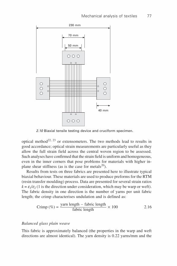
Mechanical analysis of textiles 77
optical method22, 23 or extensometers. The two methods lead to results ingood accordance; optical strain measurements are particularly useful as theyallow the full strain field across the central woven region to be assessed.Such analyses have confirmed that the strain field is uniform and homogeneous,even in the inner corners that pose problems for materials with higher in-plane shear stiffness (as is the case for metals20).
Results from tests on three fabrics are presented here to illustrate typicalbiaxial behaviour. These materials are used to produce preforms for the RTM(resin transfer moulding) process. Data are presented for several strain ratiosk = e1/e2 (1 is the direction under consideration, which may be warp or weft).The fabric density in one direction is the number of yarns per unit fabriclength; the crimp characterises undulation and is defined as:
Crimp (%) = yarn length – fabric length
fabric length 100¥ 2.16
Balanced glass plain weave
This fabric is approximately balanced (the properties in the warp and weftdirections are almost identical). The yarn density is 0.22 yarns/mm and the
70 mm
50 mm
230 mm
40 mm
2.10 Biaxial tensile testing device and cruciform specimen.

Design and manufacture of textile composites78
crimp is 0.4%. The individual yarns have slightly non-linear tensile behaviourbecause fibre cohesion in the yarn is not particularly efficient and the filamentsare not rigorously parallel. The tenacity of the glass yarns is 350 N and theirstiffness is 38 KN. Tension versus strain curves for the fabric are highly non-linear at low forces and then linear for higher loads (Fig. 2.11a). This non-linearity is a consequence of non-linear geometric phenomena occurring atlower scales, more precisely straightening at the mesoscale and compactionat the microscale. This non-linear zone depends on the prescribed strainratio, which illustrates the biaxial nature of the fabric behaviour. The non-linear zone is largest for tests in which displacement in the other direction isfree (i.e. uniaxial tests, k = 0). Here the yarns tend to become completelystraight under very low loads. Once the yarns in one direction become straight,the behaviour of the fabric is very similar to that of the yarn alone. The valueof the strain corresponding to this transition is representative of the fabriccrimp in the loading direction. The experimental results are highlyreproducible24, 25. From the tension–strain curves for different strain ratios itis possible to generate the experimental biaxial behaviour surface (Fig. 2.11b).
Balanced carbon 2 ¥ 2 twill weave
This balanced fabric is made of yarns composed of 6000 high-strength carbonfibres. In both warp and weft directions the yarn density 0.35 yarns/mm.Their tenacity is 420 N, and their uniaxial tensile behaviour is approximatelylinear (Fig. 2.12a). The fabric crimp is 0.35%. Biaxial tensile curves fordifferent strain ratios are presented in Fig. 2.12(a), and the tension surface isshown in Fig. 2.12(b). Although the yarns exhibit linear behaviour, the tensileforce versus strain behaviour of the fabric is highly non-linear at low loadsand then linear at higher loads. The non-linearity decreases as k is increased,in a similar manner to the glass plain weave fabric. Failure has been reachedfor e = 0.8% (k = 1)25 while the non-linear zone extends to approximately0.3%. Consequently, when a woven material is loaded, for instance duringforming, a major part of the fabric is in a state where its behaviour is highlynon-linear; it is, then, important to describe this non-linearity in the mechanicalbehaviour.
Highly unbalanced glass plain weave
The stiffness of the weft yarn of this fabric is 75 kN per yarn and that of thewarp is 8.9 kN per yarn. Consequently the fabric is very unbalanced. Thebehaviour of the fabric is thus significantly more non-linear than that of theindividual yarns. The two warp and weft behaviour curves (and surfaces) aredifferent (Figs 2.13a&b). The weft, which is much more rigid, has a behaviourthat is influenced very little by the warp strain. The tension surface is obtained
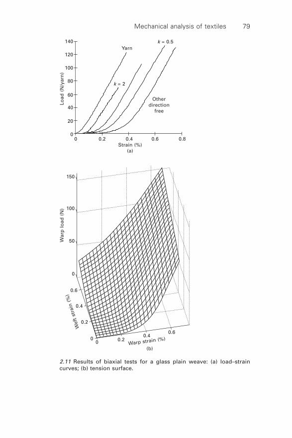
Mechanical analysis of textiles 79
Load
(N
/yar
n)
140
120
100
80
60
40
20
00 0.2 0.4 0.6 0.8
Strain (%)(a)
k = 0.5Yarn
k = 2
Otherdirection
free
War
p l
oad
(N
)
150
100
50
0
0.6
0.4
0.2
0
Wef
t st
rain
(%
)
0 0.20.4
0.6
Warp strain (%)
(b)
2.11 Results of biaxial tests for a glass plain weave: (a) load–straincurves; (b) tension surface.

Design and manufacture of textile composites80
Load
(N
/yar
n)
250
200
150
100
50
00 0.2 0.4 0.6
Strain (%)(a)
k = 0.5
Yarn
k = 2
Otherdirection
free
k = 1
2.12 Results of biaxial tests for a carbon 2 ¥ 2 twill weave: (a) load–strain curves; (b) tension surface.
War
p l
oad
(N
)
250
200
150
100
50
0
Wef
t st
rain
(%
)
0.6
0.4
0.2
00 0.2
0.40.6
Warp strain (%)
(b)

Mechanical analysis of textiles 81
by a straight translation in the warp strain direction. In contrast, the warpstrain depends strongly on the weft strain.
2.3.4 Analytical models
The biaxial experiments described above are rather difficult to perform andit is convenient to use simplified analytical models to predict the mechanicalbehaviour of the fabric from parameters related to the weave structure andthe mechanical characteristics of the yarns. Such models can be very fast andcan allow the influence of material parameters to be examined. Many modelshave been proposed in the textile science literature18, 26–29. Here the well-known Kawabata model18 is described, and a second model that is consistentwith the geometry of the woven fabric is presented.
TestsPredictions
k = 1k = 0.5
k = 2Weft
Freewarp
direction
0 0.25 0.5 0.75 1Strain (%)
(a)
Load
(N
/yar
n)
50
40
30
20
10
0
TestsPredictions
k = 1
k = 0.5
k = 2
Warp
Freeweft
direction
0 0.1 0.2 0.3 0.4 0.5 0.6 0.7Strain (%)
(b)
Load
(N
/yar
n)
250
200
150
100
50
0
2.13 Results of biaxial tests for an unbalanced glass plain weave:(a) weft load–strain curve; (b) warp load–strain curve.

Design and manufacture of textile composites82
Kawabata model
In this model, yarns within a plain weave are described by straight lines asshown in Fig. 2.14. From the geometry of the mesh the following equationcan be derived for the strain in each yarn direction:
efa = {4[e0a + (–1)awa]2 + L02
a (1 + ea)2}1/2 ( + 4 ) – 102
02 –1/2L ea a
2.17
The angle between each yarn and x3 is:
cos qa = 2[e0a + (–1)awa]{L02
a (1 + ea)2 + 4[e0a + (–1)awa]2}–1/2
2.18
2.14 Geometric representation of a plain weave in Kawabata’s model.
In the above, a (= 1 or 2) refers to the yarn direction, and wa is the yarndisplacement in the x3 direction. Other symbols are defined in Fig. 2.14.Equilibrium conditions and the projection of the loads onto the fabric meanplane leads to:
T Tf1
1 f1
2 cos = cos q q Taa = Tfa sin qa Fc = 2 fT a cos qa 2.19
where Fc is the compressive force between yarns along x3. The tensile behaviourof each yarn is given by:
T gf f = ( )a ae 2.20
A large number of studies have been published concerning the mechanicsof yarn compression14, 18, 29–32, and this is discussed in the context of fabriccompaction in section 2.4. Here an empirical compaction law is used, whichis different from that proposed by Kawabata18:
x3
x2
q01
P02
q02
P01x1Mean planeof the fabric
L02
e02
e01
L01

Mechanical analysis of textiles 83
f(Fc) = A[2 – exp(– BFc) – exp(– CFc)] = w1 – w2 2.21
The compaction coefficients A, B and C are identified using an inversemethod33, 34 from the biaxial test at k = 1.
The system of equations given above can be reduced to one non-linearequation depending on transverse displacement, and can be solved by dichotomyif strains are imposed. If loads are known, it is necessary to solve the wholesystem; an iterative method (e.g. Broyden) can be used efficiently. Goodagreement between the model and experimental results for different valuesof k is demonstrated in Fig. 2.15. Additional results for the fabrics presentedin section 2.3.3 are given by Buet-Gautier & Boisse25.
2.15 Comparison between Kawabata’s model and experimental data fora glass plain weave.
ExperimentModelling
Yarn
k = 2
k = 1
k = 0.5
0 0.1 0.2 0.3 0.4 0.5 0.6Strain (%)
120
100
80
60
40
20
0
Load
(N
/yar
n)
This model is simple and efficient. However, the 3D geometry of theyarns built on the straight segments penetrate through each other, and inorder to obtain good results as shown in Fig. 2.15 the values of parametersA, B and C are not consistent with physical values for the fabric. The goal ofthe next model is to avoid penetration of the yarns (to be geometricallyconsistent) and to work with physical values.
A geometrically consistent yarn model for fabric tensile biaxial behaviour
Here yarn longitudinal sections are curved lines with surfaces that are inconsistent contact with each other at yarn crossovers. Yarn cross-sections aredefined by the intersection of two circular arcs with different diameters.Between yarn crossovers, the yarns are assumed to follow straight paths.

Design and manufacture of textile composites84
Consequently, the yarn paths are represented by circular arcs and straightsegments (Fig. 2.16). The geometry is defined in the general case (unbalancedfabric) by a set of seven material parameters. It is convenient to measure forthe warp (a = 1) and weft (a = 2) direction, the crimp ea, the intervalbetween two yarns aa and the yarn width ca. The last parameter required isthe thickness of the fabric w. It can be shown that the solution of this systemcan be reduced to two non-linear equations giving ja1:
tan 4 – 12
( – )cos
– = 11
2–1 2
1/2
j ja aa a
aa a aL
a ca c c¢ ¢
¢ ¢ ¢ÈÎÍ
˘˚
ÏÌÓ
¸˝˛
2.22
where a ¢ = 3–a. If the fabric is balanced, only three parameters (crimp, yarnwidth and interval between two yarns) are necessary to define the wholegeometry. For the balanced glass plain weave presented in Fig. 2.11, thegeometric measurements are ca = 3.80 mm, aa = 4.55 mm and ea = 0.40%.The geometric model leads to ja1 = 0.134, ca = 2.30 mm, ba = 0.130 mm andw = 0.710 mm. These calculated quantities agree well with their physicalmeasurements, for example the fabric thickness w. The 3D geometry obtained
z y
x
M22
M21M10
M20
M11
M12
(a)
S21
S22
Mean line(O22, R22, j 22)
M12
M11
M10
zG1
j 11
R11
O11
z01
b22
b21
b2
ha
w
b1
(b)
2.16 Geometry of the consistent model (a) and section through themodel along one yarn direction (b).

Mechanical analysis of textiles 85
can be used directly for generation of finite element meshes, as will bedescribed in the following section.
The relations between the two strains and tensions in the warp and weftdirections are obtained from equilibrium in the deformed configuration:
Tfa = PRa1 Ra¢1 ja1 T
aa = Tfa cos j1a 2.23
where P is the contact pressure between crossing yarns. Axial strains in theyarn direction (which are assumed to be small) and the strains in the planeof the fabric are respectively:
e a a a
af
0
0 =
– L LL
e aaa a
a = 1
2
– 202
02
a a
a
Ê
ËÁ
ˆ
¯˜ 2.24
where the subscript 0 indicates the initial value (prior to loading). The tensilebehaviour of the yarns is given by eqn 2.20. Transverse compaction stiffnessis defined by relating the parameter r = |z2 – z1|, which describes the relativedisplacement between yarn paths, with the loads on the mesh. As suggestedabove, this stiffness depends both on the compaction state and the yarntensions:
r A e eC T T
= 2 – – –BSP –2
( + )f1
f2È
Î͢˚
2.25
where S is the yarn contact surface area. Considering the difficulty in performinga simple test to measure compaction of the yarn, the coefficients A, B and Care again determined by an inverse method using the result of the biaxial testfor k = 1.
If a strain state of the fabric (e11, e22) is prescribed, the equations in thedeformed state give the two warp and weft yarn tensions (T11, T22). It can beshown21, 35 that this set of equations can be reduced to a non-linear system oftwo equations that can be solved using an iterative (Newton) method. Thetension surface obtained in the case of the balanced plain weave glass fabricis compared with the experimental surface in Fig. 2.17. Both surfaces are ingood agreement, particularly at low strains where non-linearity is mostpronounced.
2.3.5 3D finite element analysis of the unit cellunder tension
3D finite element (FE) analysis is an alternative to the two previous approachesto determine the biaxial tensile surfaces for fabric reinforcements. This givesinformation on local phenomena that influence the global fabric mechanicalbehaviour. It can be used before fabrication to define the geometricalcharacteristics and the types of yarn for a fabric in order to obtain the desired

Design and manufacture of textile composites86
2.17 Tensile behaviour surface for balanced glass plain weave:(a) experimental and (b) geometrically consistent model prediction.
War
p l
oad
(N
)
150
100
50
0
Wef
t st
rain
(%
)
0.6
0.4
0.2
00 0.2 0.4 0.6
Warp strain (%)(a)
War
p l
oad
(N
)
150
100
50
0
Wef
t st
rain
(%
)
0.6
0.4
0.2
00 0.2 0.4 0.6
Warp strain (%)(b)

Mechanical analysis of textiles 87
mechanical properties. This is particularly interesting for complex fabricsmanufactured in small quantities and used in highly demanding structuralapplications such as aerospace components. In addition the FE approachallows the influence of material parameters (e.g. crimp, yarn density, weavepattern) on the biaxial mechanical properties of the fabric to be analysed indetail36.
The yarn is composed of a large number of fibres with small cross-sectionsthat are very flexible and can slide in relation to each other. Consequentlyyarn mechanical behaviour is highly non-linear, and exhibits very low rigidityin all directions other than parallel to the fibres. Furthermore, the transversestiffness depends on yarn compaction and tension. The equivalent materialused in 3D FE analysis must account for this behaviour. This can be achievedusing an elastic orthotropic model where the principal frame is defined withdirection 1 parallel to the yarn, with very small shear moduli (G12, G13, G23)and Poisson ratios (n12, n13, n23), and with low transverse moduli (E2, E3) incomparison with the longitudinal modulus (E1). Because local geometricnon-linearities are of primary importance, the simulation must be performedusing large strain theory. Since the axial (1 direction) and transverse moduliare very different, it is important to specify the mechanical characteristics inthe appropriate directions during the analysis. Therefore, the yarn stiffnessesare prescribed in material directions, i.e. linked to the finite elements in theircurrent position. In each of these material directions, hypoelastic behaviouris considered.
The longitudinal modulus may be constant or strain dependent, and canbe determined by tension tests on single yarns. As already noted, yarncompaction plays a major role in the deformation of woven fabrics. In thecurrent FE-based approach, local values of the mechanical properties areneeded, so that to model compaction the transverse modulus E3 is required.When the yarns are under tension, it can be observed that it is more difficultto compress them. It is therefore necessary to take this tension into account.Here, yarn compaction is represented by the evolution of the transversemodulus, which increases if transverse and longitudinal strains increase:
E E E n m3 0 33 11 = + | |e e e 2.26
where E0, m and n are three material parameters. Ee is the transverse Young’smodulus in the unloaded state, which is almost zero for the fabric yarnsdescribed in section 2.3.3. Equation 2.26 is consistent with results given byglobal yarn compression models for the evolution of the yarn thickness30, 31.When loading starts, the transverse stiffness increases because the voidsbetween fibres are reduced. Finally, the stiffness tends to an asymptoticvalue, which is very large in comparison with the value at low strain. As forthe analytical models presented above, an inverse method33, 34, 36 was used todetermine the parameters E0, m and n, using the results for a biaxial test with

Design and manufacture of textile composites88
k = 1. In this 3D simulation of the woven unit cell, a numerical difficultycomes from the very large difference between weak (or zero) values of somemoduli (particularly shear modulus) and the modulus in the direction of theyarn. This can result in spurious zero energy modes. The hourglass controlmethod, developed for finite elements with reduced integration, is used hereto avoid this problem37, 38. A master–slave approach is used to model contactbetween the yarns. It has been observed that contact non-linearities are importantfor the twill weave, but less so for the plain weave.
Figure 2.18 presents the unit cell mesh for the carbon 2 ¥ 2 twill weave(30 000 degrees of freedom), as described in section 2.3.3 The tensile behavioursurface obtained from computations under biaxial tensile loads with differentstrain ratios is also shown. This is in good agreement with the surfacedetermined by experiments (Fig. 2.12); similarly good agreement betweenFE predictions and experimental data was obtained for the other fabricsdescribed earlier21. Curves obtained from FE analysis are included in thegraphs in Fig. 2.13 (dotted lines) for the unbalanced fabric, again demonstratinggood agreement.
The 3D FE analyses show that yarn compaction is extremely important inmost cases. This is particularly evident under equal biaxial strains (i.e. k =1), where the yarn compaction (logarithmic) strain reaches a maximum valueof 40% for the glass plain weave (Fig. 2.19). In contrast, under uniaxialloading (k = 0), compaction is negligible: the stretched yarn becomes straightwhile the undulation of the free yarn increases (Fig. 2.19a).
The 2.5D carbon fabric presented in Fig. 2.20 is used in aerospace structuralcomponents. The weave pattern is such that the weft yarns cross two warplayers, so avoiding delamination between the different plies. The FE modelpresented in Fig. 2.20 has 53 000 degrees of freedom. The warp yarns areinitially straight. This explains why biaxial tests give the same response inthe warp direction for different strain ratios, so that the tensile behavioursurface is flat (Fig. 2.20b). On the other hand, the response in the weftdirection is non-linear and depends on the strain ratio (Fig. 2.20c). Given thecomplexity of such fabric reinforcements, 3D FE simulations can facilitatefabric design so that the appropriate type of yarn and weave pattern for agiven application can be determined before fabric manufacture. Results ofcomputations for other fabrics are given by Boisse and coworkers21, 36.
2.4 Compaction
2.4.1 Importance of compaction in the processing textilepreforms and composites
The widespread use of textile preforms and reinforcements for compositesmanufacturing results from the easy handling of large quantities of fibres

Mechanical analysis of textiles 89
(a)
Wef
t st
rain
(%
) 0.6
0.4
0.2
00 0.2
0.40.6
Warp strain (%)
(b)
250
200
150
100
50
0
War
p l
oad
(N
)
2.18 3D finite element analyses for biaxial tensile behaviour ofcarbon 2 ¥ 2 twill weave. (a) FE mesh and (b) predicted tensilebehaviour surface.

Design and manufacture of textile composites90
Warpdirection
Weftdirection
(a)
(b)
(c)
23%
40%27%
2.19 Yarn compaction during tensile loading of a plain weave, forstrain ratios of (a) k = 0 and (b, c) k = 1.
offered by these material forms, which make fast and economical productionpossible. Despite lower costs, stringent imperatives on processing andperformance are nonetheless present when manufacturing composites fromtextiles. Preforms must be processed in a configuration that eases manufacturingand maximises the properties of the final part.
In RTM (section 5.3.1), the injection of the resin through the preform iseased by low fibre volume fractions. These must be kept within a certainrange, above a minimum value in order to prevent movement of the preformin the mould upon injection and below a maximum value to ensure that resinflows at sufficiently high rate under practicable injection pressures. Finalparts must feature high fibre volume fractions as this ensures minimal resinusage and high specific properties, as well as limiting the possible occurrenceof resin-rich areas.
Similar considerations apply to VI (vacuum infusion, section 5.3.2). Inthis process the vacuum level and the design of the mould and gates affectthe thickness at each point of the part, in its final state and at all times duringprocessing. In turn the thickness affects preform permeability, flow, fillingdynamics and pressure distribution. Thickness and compaction behaviour ofthe textile reinforcement have a major influence on process kinetics for VI.
Compaction behaviour also plays an important role in the stamping oftextile-reinforced thermoplastic composites. Here the reduction in thicknessis an integral part of the manufacturing cycle, and must be timed accordingly.Initially, any air must be evacuated by flowing along and/or between solidfibres. Then the viscosity of the polymer (present as fibres or in partly

Mechanical analysis of textiles 91
Warp
Weft
(a)
Wef
t lo
ad (
N)
200
150
100
50
0
War
p st
rain
(%
)
0.6
0.4
0.2
00
0.20.4
0.6
Weft strain (%)(c)
War
p l
oad
(N
)
400
300
200
100
0
Wef
t st
rain
(%
) 0.6
0.4
0.2
00 0.2 0.4 0.6
Warp strain (%)(b)
2.20 3D finite element analysis for biaxial tensile behaviour of a 2.5Dfabric: (a) FE mesh and (b, c) predicted tensile behaviour surfaces.

Design and manufacture of textile composites92
consolidated form) is lowered throughout the preform, so that thoroughconsolidation can take place under increased compaction forces. Critically,these operations must be completed within a minimal cycle time. The thermalbehaviour of the material throughout the cycle depends on the imposedcompaction level. Knowledge of the fibre volume fraction in a part beingprocessed is also critical to minimising voids.
Textiles in their unloaded state have a low fibre volume fraction (typicallybetween 10 and 25%39) which must be increased during processing. Thefinal fibre volume fraction and the rates at which it is increased are generallycrucial to the economic production of quality parts. Hence control of thecompaction is essential.
Predictive simulation tools for composites manufacturing processes arebecoming increasingly available (see Chapters 4 and 7). Accurate predictionsrequire accurate data, including compaction data. However, the usefulness ofsuch compaction data extends beyond process modelling and control.Knowledge of the compaction behaviour is equally important to thespecification of manufacturing equipment and textile reinforcements for RTM.Process engineers need to know what forces are involved in bringing a preformto a target fibre volume fraction, and which textiles may be most amenableto this. Similarly, when selecting a vacuum pump for VI moulding one needsto know what preform thicknesses can be achieved for a given port set-upand part dimensions, so that the manufacturing operation can be designedappropriately and operated with confidence.
The precise scope of this section is detailed below, followed by a descriptionof the phenomena covered here. Further information on the effect of diverseparameters that relate to industrial situations is presented, and practicalrecommendations are made. While the information applies to any manufacturingprocess where textile reinforcements are used, throughout this section theconcepts and their practical consequences are discussed for three processes,namely RTM, VI and thermoplastic stamping.
2.4.2 Scope of the section
This section describes the behaviour of textile reinforcements subjected tocompaction forces normal to their plane. The focus is on the relation betweenthe force F applied to the textile and its thickness h, which can be convertedrespectively to a pressure P by dividing by the projected area A, and to a fibrevolume fraction vf.
In manufacturing, pressure is typically applied between the two rigidsurfaces of a mould (RTM, stamping, etc.) or between a lower rigid tool anda flexible membrane (VI, diaphragm forming, etc.). In this section the pressurerefers to the force applied on a textile compacted between two platens offinite area. The pressure is obtained by dividing the value of the force by the

Mechanical analysis of textiles 93
area of the platens, assuming that the textile sample has the same dimensions.Textiles are made of yarns, which in turn are made of fibres. As it is transmittedthrough the textile, the externally applied force is actually split into numeroussmall forces that are transmitted at the numerous points of contact betweenindividual fibres. Therefore, the concept of an average pressure that is constantover the surface of the platens is an approximation. A more detailed investigationwould reveal higher pressures on the yarns and no pressure in the empty gapsseparating them (Fig. 2.21). The pressure distribution on any given planecutting through the material would reflect the geometry of the preform onthat plane, with pressure levels on individual yarns being significantly higherthan the average applied pressure. Here the compaction pressure is definedas the applied force divided by the area of the platens, including the yarnsand the empty volumes defined between them.
P
Averagepressure
Localpressure
2.21 Definitions of local and average pressure during textilecompaction.
The other variable recorded in a compaction test is the preform height(thickness), which is subsequently expressed as a fibre volume fraction. Thereason for this is that preforms can be made of any number of textile layers.A given preform will often feature varying numbers of textile layers indifferent locations, as well as diverse combinations of different textiles.Using a single relationship between the applied pressure and the resultingfibre volume fraction is simpler and more general. Also, the fibre volume

Design and manufacture of textile composites94
fraction of a part is often more critical to designers than the thickness.However, although the concept of a fibre volume fraction applied to a singlelayer of textile compacted between two rigid platens is unambiguous, realpreforms are generally made of more than one textile layer. In such cases thevolume, or thickness, occupied by each layer is not precisely defined andindividual layers typically run into each other. Fibres from a given layer canlodge themselves between fibres from another layer, and at a larger scale thepeaks and valleys formed, say, by a woven textile can either fill each otheror not, (Fig. 2.22). This phenomenon is known as nesting and affects the wayin which the applied force is transmitted through textile layers.
2.22 Illustration of nesting between fabric layers – no nesting (top)and maximum nesting (bottom).
Experiments have shown that the compaction behaviour of multilayerstacks of a given textile differs from that of a single layer of the samematerial39. While a single relation between P and vf for a given textile maybe used as a guideline, in simulation one should ensure that the data representthe actual lay-up envisaged for production, especially when a high-fibrevolumes fraction is required. Furthermore, properties such as in-planepermeability of preforms or bending stiffness of composites depend on therelative thickness of individual textile layers. Preforms are sometimes built

Mechanical analysis of textiles 95
with random mats located at their core or distributed through the thickness,and enclosed between layers of directional reinforcements. Such preformswill show high in-plane permeability without major reductions in their specificbending stiffness if the compaction of the random mats is controlled. Thereader should note that European Standard BS EN ISO 5084:1997 ‘Textiles– Determination of thickness of textiles and textile products’, which supersedesBS 2544, involves a static test where the textile is subjected to one nominalload only. The evolution of vf as a function of P is not supplied by the test.
Compaction data such as those presented here are usually gathered fromtests where platens are parallel and textiles are flat and normal to the compactionaxis. A typical rig used to perform such tests is illustrated in Fig. 2.2340.
2.23 Testing fixture for reinforcement compaction40.
A
B
C
D
E
F
G

Design and manufacture of textile composites96
Textile layers are compacted between platens A and C. Other items B to Gin the figure are used to perform compaction tests on samples saturated influid, as discussed later in the text. The two platens are mounted to the ramand fixed traverse of a universal testing machine and the ensemble is loaded,usually at a constant displacement rate in the order of 1 mm/min. Calibrationtests performed with an empty rig allow the subtraction of the deformationof the rig from the total deformation at a given force, ensuring that only thecompaction of the textile layers is recorded. The sample is compacted eitherto a predetermined load or to a predetermined fibre volume fraction, dependingon the information sought. Upon reaching this state, a number of things mayhappen. The displacement will be held constant to record the relaxation at aconstant fibre volume fraction, or the force will be held constant to recordcompaction creep, or the sample will be unloaded at the same rate in orderto record a compaction hysteresis.
The surfaces of production tools are rarely flat in their entirety, and theyare not parallel where changes in thickness occur. Therefore at most pointsof the tool surfaces the compaction direction is not parallel to the axis of thepress. In simulations these factors are accommodated by projecting the pressdisplacement on the normal to the tool surface for every point of that surface,and by obtaining the corresponding pressure level. One may note that assumingthat a textile compacts along the normal to the tool surfaces is not rigorouslycorrect, as the actual relative motion of the surfaces includes a lateral componentto any normal that is not parallel to the axis of the press. No publishedexperimental data document this phenomenon, and hence it is usually neglected.
The term compaction can be used in the context of individual tows oryarns. Tow compaction happens when textiles are compacted, and is alsoobserved when textiles are sheared (section 2.2) and submitted to tension(section 2.3). Tow compaction is discussed in more detail in Chapter 1.While it may be possible to infer tow compaction properties from experimentsperformed on textiles through intelligent use of textile models, the focushere is industrial production. Basic compaction cycles are described, andphenomena such as behaviour upon impregnation, relaxation and unloadingare discussed. The important aspect of repeatability and statistical distributionof the data is covered, along with implications for mould design.
2.4.3 Basic compaction and relaxation curves
Figure 2.24 shows a typical compaction and unloading cycle for a stack oftextile reinforcements. In this case the distance between platens was reducedat a constant rate of 0.5 mm/min, held constant for 1 min and returned to itsinitial value at the same rate. The curve shows the evolution of the compactionpressure P as a function of the average fibre volume fraction vf for six layersof a woven textile; vf varies between 0.40 and 0.60 and the maximum pressure

Mechanical analysis of textiles 97
is 1.0 MPa or 10 bar; such high compaction pressures represent a practicalmaximum. The compaction part of the cycle can be characterised by aninitial fibre volume fraction vf,o which relates to the unloaded textile, arepresentative fibre volume fraction vf,r read at a predetermined pressurelevel, and an average stiffness defined over part of the loading curve wherepressure levels are significant. The curve shows that compaction pressure Pbuilds up rapidly with vf and that over the range of fibre volume fractionsused in production parts, a small increase in vf requires a large increase inpressure.
As one aims at maximising the fibre volume fraction in commercial parts,textiles are often compacted to levels where P increases very rapidly with vf,making knowledge of the compaction behaviour critical in selecting a press.In processes such as RTM the press must equilibrate the compaction pressureas well as the pressure of the resin injected in the tool. Slower injection rateslead to longer production times but allow marginally higher fibre volumefractions for a given press; such aspects must be considered carefully whendesigning production equipment. The resistance to changes in vf withfluctuations in P is advantageous in VI as small fluctuations in vacuumlevels do not affect the reproducibility of local part thicknesses. However, itshould be pointed out that vf is more sensitive to P at the lower levels ofpressure involved in that latter process. Finally, it is generally easier tocontrol the stamping of thermoplastics when conducted under a membraneas opposed to a positive displacement press; this is important especially as
Co
mp
acti
on
pre
ssu
re P
1.0
0.8
0.6
0.4
0.2
0.00.35 0.40 0.45 0.50 0.55 0.60 0.65 0.70 0.75
Fibre volume fraction Vf
2.24 Typical compaction and unloading curves for a stack of plainweave reinforcements, tested at a constant displacement ratecompaction test (pressure in MPa).

Design and manufacture of textile composites98
achievement of low void content requires accurate timing of heating andcompaction.
The dotted line in Fig. 2.24 corresponds to the relaxation step where thedistance between platens is held constant, and to load removal. The mostprominent feature is that the two curves for loading and unloading do notsuperimpose, hence the behaviour is not elastic. A practical consequence isthat if vf is overshot, say in preform stamping, the properties of the finalassembly will be altered. For example, if a RTM preform targeted at a fibrevolume fraction of 50% reached a value of 55% during its production(preforming) it would produce lower compaction pressures upon closure ofthe actual RTM mould (constant thickness), possibly resulting in a displacementof the preform upon resin injection. However, the same phenomenon canhave fortuitous consequences. In VI compaction pressure is highest when thepreform is dry, and it is progressively reduced behind the flow front. Pre-compacted preforms show reduced spring back for the same compactionpressure, hence higher fibre volume fractions may be reached in the finalparts. More generally, energy is absorbed when a textile is compacted, itsstructure is altered, and in most cases it will not return to its initial height.
Figure 2.25 illustrates a typical time relaxation curve. The curve showsthe evolution of P with time t when the distance separating the platens is heldconstant after the initial compaction. Once a certain maximum pressure levelis reached and platen travel is stopped the pressure reduces. If after a certain
0 50 100 150 200 250 300 350 400Time (s)
No
rmal
ised
co
mp
acti
on
pre
ssu
re
1.2
1.0
0.8
0.6
0.4
0.2
0.0
2.25 Typical pressure relaxation curve, where the pressure ismeasured as a function of time with the reinforcement held at aconstant thickness.
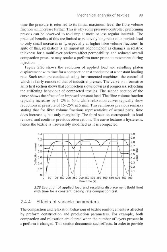
Mechanical analysis of textiles 99
time the pressure is returned to its initial maximum level the fibre volumefraction will increase further. This is why some pressure-controlled preformingpresses can be observed to re-clamp at more or less regular intervals. Thepractical benefits of this are limited as relatively long relaxation periods leadto only small increases in vf, especially at higher fibre volume fractions. Inspite of this, relaxation is an important phenomenon as changes in relativethickness for a multilayer preform affect permeability, and reduced overallcompaction pressure may render a preform more prone to movement duringinjection.
Figure 2.26 shows the evolution of applied load and resulting platendisplacement with time for a compaction test conducted at a constant loadingrate. Such tests are conducted using instrumented machines, the control ofwhich is fairly remote to that of industrial presses. The curve is informativeas its first section shows that compaction slows down as it progresses, reflectingthe stiffening behaviour of compacted textiles. The second section of thecurve shows the effect of an imposed constant load. The fibre volume fractiontypically increases by 1–2% in 60 s, while relaxation curves typically showreductions in pressure of 15–25% in 5 min. This reinforces previous remarksstating that for fibre volume fractions representative of actual parts, timedoes increase vf but only marginally. The third section corresponds to loadremoval and confirms previous observations. The curve features a hysteresis,hence the textile is irreversibly modified as it is compacted.
Def
lect
ion
(m
m)
1.4
1.2
1.0
0.8
0.6
0.4
0.2
00 50 100 150 200 250 300 350 400 450 500 550 600 650 700
Run time (s)
1.00.90.80.70.60.50.40.30.20.10
Load
(kN
)
2.26 Evolution of applied load and resulting displacement (bold line)with time for a constant loading rate compaction test.
2.4.4 Effects of variable parameters
The compaction and relaxation behaviour of textile reinforcements is affectedby preform construction and production parameters. For example, bothcompaction and relaxation are altered when the number of layers present ina preform is changed. This section documents such effects. In order to provide

Design and manufacture of textile composites100
a usable summary of general trends, the effect of parameters on a number ofvariables are considered.
For compaction the following quantities were introduced previously: theinitial fibre volume fraction vf,o of the unloaded textile, the representativefibre volume fraction vf,r read at a predetermined pressure level, and theaverage stiffness defined over a set range of pressure levels. Another variablethat will be commented upon is the rate at which the rigidity of the textileincreases as the textile is compacted; this will be referred to as the stiffeningindex. For relaxation, a reduction in compaction pressure is observed at aconstant thickness and therefore the reduction in pressure observed after aperiod of 5 min will be commented upon; this will be referred to as thepressure decay.
The parameters investigated for both compaction and relaxation are thenumber of layers (NOL) and saturation by a fluid (SAT). In the latter case,experimental observations show that the compaction behaviour of a set numberof layers of reinforcement differs if the reinforcement is compacted dry orsaturated with resin. Considering VI for example, this means that when theresin front reaches a given point of the preform, the compaction behaviour atthat point changes, effectively becoming less stiff. This can result in a localreduction in thickness at the flow front, a phenomenon usually visible to thenaked eye. Additional parameters will also be commented upon. Forcompaction, the effect of the number of cycles (NOC) applied to a preformwill be discussed. This applies to numerous practical situations such as RTMoperations where preforms are often manufactured in a separate operation tothe actual moulding.
The observed effects of the NOL on compaction are as follows. Differentauthors have reported different trends, which may be explained by the differenttextiles and pressure levels used. For some textiles compacted to higherpressures, it has been shown that stacks made of a higher number of layersare more difficult to compact to a given fibre volume fraction vf with compactioncurves progressively shifting to the left (lower fibre volume fractions), mostlyat higher pressures. At the onset of compaction multilayer stacks are easierto compact because of nesting; however, at higher pressures these preformsare usually more difficult to compact to a given vf, hence fibre volumefractions are lower for a given pressure and the curve shifts to the left. Whilevf,o usually increases with NOL, vf,r shows the opposite trend at high pressures.Therefore both the rigidity and stiffening index tend to increase with NOL(Fig. 2.27). Other authors who have used lower compaction pressures, whichare more indicative of manufacturing using VI for example, find that multilayerpreforms are easier to compact to higher fibre volume fractions. Their resultsare not contradictory as they use different pressure levels. Besides, the effectof the number of layers on the compaction behaviour is often relatively weakand some authors have observed conflicting trends.

Mechanical analysis of textiles 101
Preforms made of a higher number of layers show more relaxation inpressure at constant thickness. The pressure decay, defined as the ratio of thepressure observed after 5 mins to the maximum applied pressure, is typicallyreduced by up to 10% for thicker preforms.
The effects of compacting a reinforcement saturated in a fluid, say resin,are as follows. It should be noted that what is discussed here is quasi-staticcompaction, i.e. compaction at displacement rates that are sufficiently low torender insignificant the pressure generated by the fluid as it is squeezed outof the reinforcement stack. The phenomenon investigated in the reportedexperiments is the effect of saturation, and lubrication, on the individualcontacts between fibres where forces are transmitted. Typical results for theeffect of saturation are given in Fig. 2.28. Experiments show that saturated(vf, P) compaction curves are generally shifted to the right, that is towardshigher fibre volume fractions. The initial fibre volume fraction vf,o andrepresentative fibre volume fraction vf,r are generally higher by a few percent. As both values of the fibre volume fraction, the rigidity and stiffeningbehaviour, are generally unaffected; the compaction behaviour remainsessentially identical but marginally higher values of fibre volume fractionare observed at given values of the compaction pressure. This can be observedpractically for VI as the preform usually compacts to a slightly lower thickness(higher vf) as the flow front reaches a given position. The effect cannot beobserved easily for RTM; however, once enclosed in a mould it is thoughtthat the load on a preform will progressively reduce as a result of time
3 Layers6 Layers12 Layers
Co
mp
acti
on
pre
ssu
re (
MP
a)
2.5
2.0
1.5
1.0
0.5
0.00.40 0.45 0.50 0.55 0.60 0.65 0.70 0.75 0.80 0.85
Fibre volume fraction Vf
2.27 Textile compaction data for stacks with different numbers oflayers for a non-crimp fabric reinforcement.

Design and manufacture of textile composites102
relaxation, and that a further reduction will be observed upon impregnation.It is therefore important to use a sufficiently thick preform that will lead toappropriate initial levels of compaction pressure, in order to ensure properpositioning of the preform in the tool throughout the process.
Saturation usually has a strong effect on the relaxation part of the cycle.Saturated stacks reach somewhat higher volume fractions when compacted,and they exhibit significantly less relaxation; after 5 mins the pressure usuallyremains between 75 and 90% of its initial value. It is believed that thisbehaviour can be explained by the lubrication of fibre-to-fibre contact points.Individual fibres will slide more easily for a saturated stack and are thereforemore likely to attain a higher degree of stability for a given compactionpressure. As a result, fibres are less likely to move under pressure, exhibitingless relaxation.
The above comments are corroborated when one considers the compactionbehaviour of a preform subjected to repeated compaction cycles. Figure 2.29shows typical compaction cycles imposed on a multilayer preform; themaximum pressure level is constant at 1.0 MPa41. The figure clearly showsthat the compaction and load release curves shift to the right on successivecycles. The shift is more marked on the first repeat and progressively diminisheson successive cycles. Both vf,o and vf,r increase, and this increase is typicallymore marked than those observed with saturated preforms, notably on thefirst cycle. The fibre volume fraction observed at higher pressures increases,but less than it does at low fibre volume fractions. Consequently, the rigidityand stiffening index also increase markedly on successive cycles. Suchbehaviour is observed over a number of cycles; the difference over successive
Co
mp
acti
on
pre
ssu
re (
MP
a)
1.2
1.0
0.8
0.6
0.4
0.2
0.0
DrySaturated
0.40 0.45 0.50 0.55 0.60 0.65Fibre volume fraction (Vf)
2.28 Effect of fluid saturation in textile compaction behaviour.

Mechanical analysis of textiles 103
cycles diminishes progressively but does not appear to stabilise, at least over50 cycles. This, along with the fact that an important hysteresis is observedon each cycle, points to the fact that reorganisation of the fibres happens asthe textile is compacted and keeps happening on successive cycles. While oflittle practical importance for processes such as RTM, this provides goodinsight on the behaviour of textile reinforcements. Furthermore, this behaviourmay have consequences for VI where the preform is compacted under vacuum,unloaded upon injection and possibly reloaded during bleeding.
The above trends can be put in perspective by looking at the naturalvariability observed upon compaction of nominally identical stacks of textilereinforcements. Figure 2.30 shows typical data scatter for 12 identicalcompaction samples. Here the textile reinforcements were compacted to alower maximum pressure of 0.1 MPa, which usually leads to more scatter fora given pressure. However, and although the trends discussed above emergeclearly from carefully conducted experiments, the amplitude of the scattershown in Fig. 2.30 is similar to some of the weaker trends, say for examplethe effect of the number of layers on compaction curves. Actual productionequipment is generally not selected for operation at its limit; in spite of this,variability data should be included when considering necessary forces andcontrol accuracy.
Co
mp
acti
on
pre
ssu
re (
MP
a)
1.0
0.8
0.6
0.4
0.2
0.00.35 0.40 0.45 0.50 0.55 0.60 0.65 0.70 0.75
Fibre volume fraction (Vf)
Cycle 1
Cycle 11
Cycle 21Cycle 31
Cycle 41
Cycle 51
2.29 Pressure curves for successive compaction cycles applied to amultilayer plain weave preform.

Design and manufacture of textile composites104
2.4.5 Modelling
A number of authors have proposed models for the compaction behaviour oftextiles (a thorough review of these is given by Robitaille and Gauvin39).Such models usually aim to fulfil one of two objectives: phenomenologicalmodels attempt to explain the behaviour from the fundamental principles ofmechanics while empirical models provide a simple and usable representationof experimental data. Although both approaches were investigated forcompaction, no credible explanation is available for the time relaxation oftextile reinforcements and in this case a limited number of empirical modelssimply aim at quantifying the phenomenon.
The most widely known and used phenomenological compaction modelwas proposed by Cai and Gutowski14. The main concept behind this modelis that individual fibres form arches between their contact points; as compactionprogresses it is assumed that the number of contact points increases as thelength of the arches is essentially proportional to the thickness of thereinforcement being compacted. Consequently, beam bending theory dictatesthat the arches progressively become more rigid as their number increases,resulting in a marked stiffening behaviour. The authors have proposed differentequations (see equation 2.5 for an alternative example), but perhaps the mostgeneral is expressed as:
P A
vv
v v
comp s
f
fo
f fa
4= – 1
1 –
1
ÊË
ˆ¯
ÊË
ˆ¯
2.27
Co
mp
acti
on
pre
ssu
re (
MP
a)
0.12
0.10
0.08
0.06
0.04
0.02
0.000.35 0.40 0.45 0.50 0.55 0.60 0.65
Fibre volume fraction (Vf)
2.30 Compaction data for 12 tests conducted on samples of the samereinforcement, showing the significant data scatter that is to be expected.

Mechanical analysis of textiles 105
where vf,o and vf,a are the initial and maximal fibre volume fractions, As is anempirical constant, and vf and Pcomp are the fibre volume fraction and thecompaction pressure. It should be noted that owing to its nature andphenomenological origin the model uses the fibre volume fraction as theindependent variable, which is not ideal; the form of the equation can makethe extraction of a fibre volume fraction at a given compaction pressureawkward.
Gutowski’s work provides very interesting and valuable insight into thecompaction phenomenon; however, it really applies to homogeneous assembliesof parallel fibres. Results of experiments conducted on reinforcements ofvarious architectures clearly show that the textile structure, or the way inwhich tows or yarns of various sizes are assembled into a planar assemblythat is homogeneous and continuous at the macroscopic scale, but heterogeneousand discontinuous at the mesoscopic scale, strongly affect the behaviour. Itis possible, for example, to classify compaction curves for random mats,woven textiles and stitched directional reinforcements into relatively distinctgroups; this important point is discussed further in the following paragraphs.Furthermore, getting a good fit for the diverse coefficients of the models canbe challenging in some cases, and values obtained for coefficients with aclear physical meaning such as vf,o and vf,a often do not match reality whenthe model is applied to heterogeneous textiles. The model was really developedfor assemblies of aligned fibres and the lack of correspondence between thefitted and experimental values reduce its attractiveness to some extent.
The alternative consists of using empirical models. While studying changesin the values of the coefficients of such models with experimental parametershelps in identifying trends, there is no pretence at a quantitative, mechanicaldescription of the phenomena involved in the process. However, this can becompensated by the fact that similar models can be used to describe relaxationbehaviour, enabling both phenomena to be included in process simulationsand treated in the same way. Empirical models of compaction and relaxationare not satisfactory in all circumstances. Numerous published works haveprovided remarkable phenomenological insight into compaction and otherproperties of fibre assemblies, as well as models that can represent realbehaviour for actual fibrous structures such as ropes. Finite element analysessimilar to those described in section 2.3.5 would appear to be a promisingapproach here, and this is expected to be an area of significant activity in thenear future. At this time most of these models require very significantcomputational power, but work is ongoing and in the future, more efficientmodels that can reasonably be used to support actual production of compositeparts may appear.
Most empirical models of the compaction revolve around some form ofthe power law. The authors and numerous others have used the followingexpression to fit experimental compaction data:

Design and manufacture of textile composites106
v v P Bf fo comp = ◊ 2.28
where vf,o is the fibre volume fraction recorded under a pressure of 1 Pa andB is an empirical factor called the stiffening index. Because of the mathematicalform of the equation the latter value provides a good indication of the rate ofincrease of the rigidity as a function of vf ; as such it is practically veryuseful. Here the pressure is the independent variable, and the equation iseasily fitted to data.
Robitaille and Gauvin39 proposed a similar model for time relaxation:
PP
C t D
o
(1/ ) = 1 – 2.29
where C is the pressure decay after 1 sec, D is the relaxation index, Po is theinitially applied pressure and P is the compaction pressure observed at timet which is the independent variable.
The above empirical formulae have allowed the formal identification ofall the trends mentioned above. The compaction model was also successfullyintegrated into a number of process simulation models. Tables of coefficientsfor both equations can be found in the literature for a range of materials39, 40
and it is very straightforward to fit experimental data to the equations. Whilethese models do not explain the physics of compaction and relaxation andone must identify the coefficients associated to each stack of reinforcementsthat may be used in production, they are very useful in practice.
A recent study further extends the benefits of the compaction model whenconsidering a number of structurally different reinforcements42. The curveshown in Fig. 2.31 is a compaction master curve, which presents the evolution
2.31 Compaction master curve, showing a relationship between stiffeningindex and initial fibre volume fraction values (equation 2.28) for a rangeof reinforcements.
Random fibresIncreasing numberof layers and cycles
Oriented fibres
0 0.05 0.10 0.15 0.20 0.25 0.30 0.35 0.40 0.45vfo
B
0.40
0.35
0.30
0.25
0.20
0.15
0.10
0.05
0

Mechanical analysis of textiles 107
of the stiffening index B as a function of the initial fibre volume fraction vf,o
for an array of reinforcements. The curve shows a fairly clear generalrelationship between the two parameters. Furthermore, all randomreinforcements are found on the left side of the curve, most woven fabricsoccupy the centre and textiles featuring highly oriented fibres (e.g. NCFs)are found on the right. Practically this translates into the fairly simple factthat random textiles initially show low fibre volume fractions and that theystiffen relatively slowly, while crimp-free assemblies of unidirectional fibresfeature high initial fibre volume fractions and stiffen very rapidly.
References
1. Blanchard P., Cao J., Chen J. and Long A.C. (co-chairs), NSF workshop on compositesheet forming, Lowell, MA, Sept 2001. http://www.mech.northwestern.edu/fac/cao/nsfworkshop/index.htm
2. Saville B.P., Physical Testing of Textiles, Cambridge, Woodhead Publishing Ltd,1999.
3. Lomov S.V., Verpoest I., Barburski M. and Laperre J., ‘Carbon composites based onmultiaxial multiply stitched preforms. Part 2. KES-F characterisation of thedeformability of the preforms at low loads’, Composites Part A, 2003 34(4) 359–370.
4. Potter K.D., ‘The influence of accurate stretch data for reinforcements on the productionof complex structural mouldings’, Composites, July 1979 161–167.
5. Skelton J., ‘Fundamentals of fabric shear’, Textile Research J., Dec. 1976 862–869.6. Wang J., Page R. and Paton R., ‘Experimental investigation of the draping properties
of reinforcement fabrics’, Composites Sci. Technol., 1998 58 229–237.7. Canavan R.A., McGuinness G.B. and O’Braidaigh C.M., ‘Experimental intraply
shear testing of glass-fabric reinforced thermoplastic melts’, Proc. 4th Int. Conf. onAutomated Composites, Nottingham, Sept. 1995, 127–138.
8. Long A.C., Rudd C.D., Blagdon M. and Johnson M.S., ‘Experimental analysis offabric deformation mechanisms during preform manufacture’, Proc. 11th Int. Conf.on Composite Materials, Gold Coast, Australia, July 1997, V: 238–248.
9. Prodromou A.G. and Chen J., ‘On the relationship between shear angle and wrinklingof textile composite preforms’, Composites Part A, 1997 28A 491–503.
10. Mohammad U., Lekakou C., Dong L. and Bader M.G., ‘Shear deformation andmicromechanics of woven fabrics’, Composites Part A, 2000 31 299–308.
11. Souter B.J., Effects of fibre architecture on formability of textile preforms, PhDThesis, University of Nottingham, 2001.
12. Kawabata S., Niwa M. and Kawai H., ‘The finite-deformation theory of plain-weavefabrics Part III: The shear-deformation theory’, J. Textile Institute, 1973 64(2) 61–85.
13. McBride T.M. and Chen J., ‘Unit-cell geometry in plain-weave fabrics during sheardeformations’, Composites Sci. Technol., 1997 57 345–351.
14. Cai Z. and Gutowski T.G., ‘The 3D deformation behavior of a lubricated fiberbundle’, J. Composite Materials, 1992 26(8) 1207–1237.
15. McBride T.M., The large deformation behavior of woven fabric and microstructuralevolution in formed textile composites, PhD Thesis, Boston University, 1997.

Design and manufacture of textile composites108
16. Harrison P., Wiggers J., Long A.C. and Rudd C.D., ‘A constitutive model based onmeso and micro kinematics for woven and stitched dry fabrics, Proc. 14th Int. Conf.on Composite Materials, San Diego, July 2003.
17. Harrison P., Yu W.-R., Wiggers J. and Long A.C., ‘Finite element simulation offabric forming, incorporating predictions of a meso-mechanical energy model’, Proc.7th Int. European Scientific Association for Material Forming Conf., Trondheim,Norway, April 2004, 139–142.
18. Kawabata S., Niwa M. and Kawai H., ‘The finite-deformation theory of plain weavefabrics Part I: The biaxial deformation theory’, J. Textile Institute, 1973 64(2) 21–46.
19. Kawabata S., ‘Nonlinear mechanics of woven and knitted materials’, in Chou T.W. andKo F.K. (eds) Textile Structural Composites, Amsterdam, Elsevier, 1989, pp 67–116.
20. Ferron G., ‘Dispositif de traction biaxiale DAX2’, Document Tech-metal, Mézières-Lès-Metz, 1992 (in French).
21. Boisse P., Gasser A. and Hivet G., ‘Analyses of fabric tensile behaviour. Determinationof the biaxatension-strain surfaces and their use in forming simulations’, CompositesPart A, 2001 32(10) 1395–1414.
22. Launay J., Lahmar F., Boisse P. and Vacher P., ‘Strain measurement in tests on fibrefabric by image correlation method’, Adv. Composite Lett., 2002, 11(1) 7–12.
23. Dumont F., Hivet G., Rotinat R., Launay J., Boisse P. and Vacher P., ‘Identificationdes caractéristiques mécaniques de renforts tissés à partir de mesures de déformationspar corrélation d’images’, Mécanique & Industries, in press (in French).
24. Buet-Gautier K, Analyse et simulation du comportement mécanique des renfortscomposites tissés, PhD Thesis, University of Orléans, 1998 (in French).
25. Buet-Gautier K. and Boisse P., ‘Experimental analysis and models for biaxialmechanical behaviour of composite woven reinforcements’, Experimental Mechanics,2001, 41(3), 260–269.
26. Anandjiwala R.D. and Leaf G.A.V., ‘Large-scale extension and recovery of plainwoven fabrics’, Textile Research J., 1991 61(11) 619–634.
27. Realff M.L., Boyce M.C. and Backer S., ‘A micromechanical approach to modellingtensile behavior of woven fabrics’, in Stokes V.K. (ed) Use of Plastics and PlasticComposites: Materials And Mechanics Issues, New York, ASME MD-Vol. 46, 1993,285–294.
28. Dastoor P.H., Ghosh T.K., Batra S.K. and Hersh S.P., ‘Computer-assisted structuraldesign of industrial woven fabrics. Part III: Modelling of fabric uniaxial/biaxialload-deformation’, J. Textile Institute, 1994 85(2) 135–157.
29. Lomov S.V., Gusakov A.V., Huysmans G., Prodromou A. and Verpoest I., ‘Textilegeometry preprocessor for meso-mechanical models of woven composites’, CompositesSci. Technol., 2000 60 2083–2095.
30. Grishanov S.A., Lomov S.V., Harwood R.J., Cassidy T. and Farrer C., ‘The simulationof the geometry of two-component yarns. Part I: The mechanics of strand compression:simulating yarn cross-section shape’, J. Textile Institute, 1997 88(2) 118–131.
31. Harwood R.J., Grishanov S.A., Lomov S.V. and Cassidy T., ‘Modelling of two-component yarns. Part I: The compressibility of yarns’, J. Textile Institute, 199788(4) 373–384.
32. Baoxing C. and Chou T.W., ‘Compaction of woven-fabric preforms in liquid compositemolding processes: single layer deformation’, Composite Sci. Technol., 1999 591519–1526.
33. Marquardt D.W., ‘An algorithm for least squares estimation of nonlinear parameters’,J. Soc. Indus. Appl. Math, 1963 11(2) 431–441.

Mechanical analysis of textiles 109
34. Schnur D.S. and Zabaras N., ‘An inverse method for determining elastic materialproperties and a material interface’, Int. J. Numerical Methods Eng., 1992 33 2039–2057.
35. Hivet G., Modélisation mesoscopique du comportement biaxial et de la mise enforme des renforts de composites tissés, PhD Thesis, University of Orléans, 1998 (inFrench).
36. Gasser A., Boisse P. and Hanklar S., ‘Analysis of the mechanical behaviour of dryfabric reinforcements. 3D simulations versus biaxial tests’, Comp. Material Sci.,2000 17 7–20.
37. Flanagan D.P. and Belytschko T., ‘A uniform strain hexahedron and quadrilateralwith orthogonal hourglass control’, Int. J. Numerical Methods Eng., 1981 17 679–706.
38. Pian T.H. and Chen D., ‘On the suppression of zero energy deformation modes’, Int.J. Numerical Methods Eng., 1983 19 1741–1752.
39. Robitaille F. and Gauvin R., ‘Compaction of textile reinforcements for compositesmanufacturing. I: Review of experimental results’, Polymer Composites, 1998 19(2)198–216.
40. Robitaille F. and Gauvin R., ‘Compaction of textile reinforcements for compositesmanufacturing. II: Compaction and relaxation of dry and H2O-saturated wovenreinforcements’, Polymer Composites, 1998 19(5) 543–557.
41. Robitaille F. and Gauvin R., ‘Compaction of textile reinforcements for compositesmanufacturing. III: Reorganization of the fiber network’, Polymer Composites, 199920(1), 48–61.
42. Correia N., Analysis of the vacuum infusion process, PhD Thesis, University ofNottingham, 2004.

110
3.1 Introduction
Virtual design and manufacture of industrial components can provide significantincreases in efficiency and reductions of cost in the manufacturing process.This factor provides strong motivation for the composites industry to developsimulation technology for continuous fibre reinforced composites (CFRC)(e.g. Smiley and Pipes 1988; O’Bradaigh and Pipes 1991; de Luca et al.1996, 1998; Pickett et al. 1995; McEntee and O’Bradaigh 1998; O’Bradaighet al. 1997; Sutcliffe et al. 2002; Lamers et al. 2002a,b; Yu et al. 2002;Sharma and Sutcliffe 2003). The overriding goal is to make CFRC materialsa more attractive option, in a market where composites are often viewed asexpensive alternatives to more traditional materials, such as metal and plastic.One of the main challenges in the simulation process is the development ofconstitutive models that can predict accurately the unique and complexrheological behaviour of viscous CFRC, including textile reinforcedthermoplastic composites and thermosetting prepreg composites.
Continuous fibre reinforced composites can be divided into uniaxial CFRCthat contain reinforcement in one direction and fabric or textile reinforcedcomposites. The constitutive modelling and associated experimental workon viscous uniaxial and cross-ply CFRC laminates (i.e. laminates consistingof multiple layers of uniaxial CFRC) have received considerable attentionover a period of more than a decade. However, until recently, relatively littleattention was paid to the characterisation and modelling of viscous textilecomposites. This situation has changed in recent years; indeed, characterisationand constitutive modelling of viscous textile composites now constitute anactive area of research.
The aim of this chapter is to provide the reader with an overview of thecurrent state of rheological modelling of viscous textile composites togetherwith the experimental methods available to characterise their rheology. Insection 3.2, a brief discussion of the deformation mechanisms involved inthe forming of viscous textile composites is given. Section 3.3 is a review of
3Rheological behaviour of pre-impregnated
textile composites
P H A R R I S O N and M C L I F F O R D,University of Nottingham, UK

Rheological behaviour of pre-impregnated textile composites 111
the constitutive modelling work for viscous textile composites. The idealfibre reinforced model (IFRM) is discussed in sections 3.3.1 to 3.3.3. Herethe term ‘ideal’ refers to fibre reinforced incompressible materials that areinextensible along the fibre direction (Hull et al. 1994). Attention is drawnto the difficulty in formulating constituent-based predictive models for viscoustextile composites using this approach. Attempts to deal with this limitationappear in the literature and these are discussed in sections 3.3.4 and 3.3.6.The inextensibility constraint has been relaxed in some models, as discussedin section 3.3.5. Section 3.4 provides a description and discussion ofexperimental test methods typically employed in characterising the rheologyof viscous textile composites. Finally, section 3.5 describes a visual analysissystem used in determining the deformation mechanisms acting during theforming of viscous textile composites over complex shaped components.This technique provides a convenient tool for evaluating the predictions ofnumerical forming codes.
3.2 Deformation mechanisms
Various deformation mechanisms can occur during forming of a sheet oftextile composite material (e.g. Cogswell 1992, 1994; Friedrich et al. 1997;Murtagh and Mallon 1997; Mallon and O’Bradaigh 2000). These deformationscan be classified according to the length scale over which they occur. Figure3.1 illustrates various macroscopic deformations. When considering a singlelayer of textile composite sheet, a single mode of deformation known asintra-ply shear, dominates; see Fig. 3.1(a). As will be shown, intra-ply shearis by far the most important and widely studied mechanism in continuummodels for textile composites. Intra-ply shear, or trellis deformation, can bevisualised by thinking of a woven composite material as a pin-jointed netmade from inextensible fibres, with the joints occurring at tow crossoverpoints. As the net is forced to deform, the tows rotate about the crossoverpoints, which results in the material shearing. This is the only mode ofdeformation considered by the IFRM (see section 3.3), and is also the onlymode of deformation modelled by kinematic draping codes (see section 4.2).
Given the relatively high tensile modulus of the reinforcement in, forexample, glass or carbon fibre-based textile composites intra-ply extension,Fig. 3.1(b), may seem an irrelevant deformation mechanism during forming(i.e. intra-ply shear should offer a much lower energy, and therefore preferable,mode of deformation). However, fibres may extend during forming withoutexcessive forces due to uncrimping of the tows (fibre bundles or yarns) in thetextile. Thus, a small degree of intra-ply extension may be expected even intextile composites with high modulus reinforcement. Recent attempts toaccount for fibre extensibility (and at the same time avoid numerical problemsassociated with the inextensibility constraint) in finite element (FE) simulations

Design and manufacture of textile composites112
have been made using different approaches (e.g. Lamers et al. 2002a; Xue etal. 2003; Yu et al. 2003) (see section 3.3.6). It is interesting to note thatrecent interest in self-reinforced polymer–polymer composites (e.g. Prosseret al. 2000; Harrison et al. 2002d) has made intra-ply extension of evengreater relevance, as tows in this type of composite have much lower modulusthan for typical woven composites.
(a)
(b)
(c)
(d)
3.1 Macroscopic deformation mechanisms during forming of textilecomposite material, including (a) intra-ply shear, (b) intra-plyextension, (c) inter-ply slip and (d) inter-ply rotation.

Rheological behaviour of pre-impregnated textile composites 113
For multilayered composites, slip between adjacent layers during formingmust also be considered, including inter-ply slip, Fig. 3.1(c) and inter-plyrotation, Fig. 3.1(d). Inter-ply slip and rotation describe the relative motionof one ply over another as components are formed from multi-ply lay-ups(e.g. Friedrich et al. 1997; Murtagh and Mallon 1997; Lamers et al. 2003;Phung et al. 2003). These modes of deformation are essential if geometrieswith double curvature are to be formed from multilayer composites withoutwrinkling, particularly when using plies of initially different orientations.
Recently, homogenisation methods have been used to predict the behaviourof representative volume elements within textiles from consideration ofindividual tow (fibre bundle) and inter-tow deformations (i.e. mesoscaledeformations). Indeed, the potential of textile modelling at the mesoscalehas been greatly enhanced recently by increases in computing power and isbecoming a growing area of interest for researchers (e.g. Hsiao and Kikuchi1999; Harrison et al. 2004a; Lomov et al. 2002; Hagege et al. 2003). Examplesof mesoscale deformations are shown in Fig. 3.2. Various distinct modes oftow deformation can be identified including tow-shear, Fig. 3.2(a), and tow-squeezing plus tow-twisting (one mode) and tow-bending (two modes) about
(a)
(b)Y
Z
X
3.2 Mesoscale deformation mechanisms during forming of textilecomposite material, including (a) tow shear and (b) tow squeezing,twisting and bending. Relative motion between tows can also occurwithin the ply, including (c) crossover shear and (d) inter-tow shear.Finally, intra-ply slip is another potential deformation mechanismand can be classified as either (e) crossover slip or (f) inter-tow slip.

Design and manufacture of textile composites114
(c)
(d)
(e)
(f)
3.2 Continued

Rheological behaviour of pre-impregnated textile composites 115
the tow axes, Fig. 3.2(b). Mesoscale tow deformations permit macroscaleforming of the textile as well as facilitating textile specific deformationssuch as mesoscale fibre buckling. The relative motion of neighbouring towsand their subsequent interaction is also an important factor when modellingtextile deformation at the mesoscale. Examples include crossover shear, Fig.3.2(c) (Harrison et al. 2002a,b; Zouari et al. 2003), which potentially induceslarge shear strain rates in the matrix fluid between superposed tows, andinter-tow shear, Fig. 3.2(d), which arises when the shear rate across tows isless than the average shear rate across the textile composite sheet (see section3.3.6).
The nature of mesoscale models means that they can include informationsuch as tow architecture, tow and inter-tow kinematics and can also possiblyincorporate so-called intra-ply slip mechanisms. Two distinct types of intra-ply slip can be identified, crossover slip, Fig. 3.2(e) (e.g. Lai and Young1999), and inter-tow slip, Fig. 3.2(f) (Harrison et al. 2004b). These mechanismsare a direct result of relative displacements between neighbouring tows andhave been observed to play an important role during the deformation oftextile composites. Intra-ply slip occurs most readily in loosely wovencomposites and in some cases can actually improve the formability of thetextile (Long et al. 2002). However, too much crossover slip can leave resin-rich regions or, in extreme cases, unwanted holes in components as the towsmove apart. Crossover slip is important during press forming and hand lay-up, while inter-tow slip is apparent during bias extension tests, Fig. 3.2(f)(Harrison et al. 2004b).
Finally, prediction of individual tow properties can be made using knowledgeof factors such as matrix rheology and fibre volume fraction, from considerationof micro-scale fibre–fluid interactions within the individual tows. Theseinteractions are illustrated in Fig. 3.3 and include both (a) intra-tow transverseshear and (b) intra-tow axial shear (see section 3.3.2).
(a) (b)
3.3 (a) Shearing the composite parallel to the fibre direction gives ameasure of the longitudinal viscosity, hL. (b) Shearing the compositeacross or transverse to the fibre direction gives a measure of thetransverse viscosity, hT. Micromechanical models based on thesefibre organisations have been developed that relate the matrixviscosity and fibre volume fraction to the two viscosities.

Design and manufacture of textile composites116
Many of the modelling approaches developed to describe the deformationsrequired to form components have as their goal the elimination of fibrebuckling (mainly in relation to uniaxial CFRC) and wrinkles. Although theprediction of these is therefore of prime importance, relatively little workhas concentrated on the development and subsequent growth of wrinkles(Hull et al. 1991, 1994; Friedrich et al. 1997; Li and Gutowski 1997;O’Bradaigh et al. 1997; Mander et al. 1997; Martin et al. 1997b; De Luca etal. 1998; Yu et al. 2003). The prediction of wrinkles is an important area forfuture work.
3.3 Review of constitutive modelling work
In this section, a review of the constitutive modelling of viscous textilecomposites is presented. Examination of the literature reveals various modellingapproaches. The first and most widely studied is that of continuum mechanics,in particular models based on the IFRM (section 3.3.1). The IFRM hasproved successful in many respects, not least in obtaining analytical solutionsto specific well-defined flow deformations. However, certain limitations ofthe theory have become apparent. These include difficulties found in model-parameter evaluation for ‘real’ textile composites through experimentalcharacterisation and problems involved in implementing these equations inFE codes.
The review of IFRMs includes work on both viscous uniaxial (section3.3.2) and biaxial (section 3.3.3) CFRC. While at first sight, the case of theuniaxial IFRM is not directly applicable to textile composites, this work isnevertheless considered for two reasons. The first is to illustrate one of themore ambitious yet desirable goals of CFRC constitutive models, that is, thedevelopment of fully predictive models based on properties such as fibrevolume fraction and resin viscosity (see also sections 3.3.4 and 3.3.6). Successin this area would dramatically reduce the need for extensive experimentalcharacterisation programmes (section 3.4). The second is because at leastone approach to textile deformation modelling, the energy summation method(section 3.3.6), is based on the uniaxial rather than biaxial IFRM.
When implementing a material model in an FE code, an importantconsideration is the effect of the kinematic constraints of the model on thenumerical calculations. The inextensibility constraint of the IFRM leads toarbitrary tensile stresses in the reinforcement directions (see section 3.3.1),stresses that can cause potential problems when calculating force equilibrium.This issue has led certain workers to develop alternative constitutive modelsfor sheet forming predictions (section 3.3.5).

Rheological behaviour of pre-impregnated textile composites 117
3.3.1 The ideal fibre reinforced model for viscous fluids
The continuum theory of the mechanics of CFRC in a solid or elastic statewas developed initially by Spencer and referred to as the elastic ideal fibrereinforced model (Spencer 1972, 1984). This work was adapted by Rogers(1989a) to the case of viscous CFRC through use of the ‘correspondenceprinciple’ of viscoelasticity. The underlying assumptions of the IFRM forviscous composites have been outlined many times previously (e.g. Hull etal. 1994; Rogers 1989a, 1990; Spencer 2000; McGuiness and O’Bradiagh1998; Mallon and O’Bradaigh 2000) and are repeated here for convenience.
As with the elastic IFRM, two important approximations are used inobtaining solutions in the stress analysis, those of incompressibility andfibre-inextensibility. These conditions can be expressed mathematically asfollows. Using D, the rate of deformation tensor which can be written incomponent form as
Dvx
v
xiji
j
j
i = 1
2 +
∂∂
∂∂
ÊËÁ
ˆ¯
3.1
where vi are the velocity components of a particle at position xi, theincompressibility condition can be written as
Dvxii
i
i = = 0
∂∂ 3.2
where the repeated suffix summation convention applies. This first familiarconstraint is often used in fluid mechanics. The second constraint of fibreinextensibility is more particular to CFRC theory. The reinforcement fibresare considered as continuously distributed throughout the material and foruniaxial reinforcement are defined at any point by a unit vector, a(x, t) or fortextile composites with two directions of reinforcement by a(x, t) and b(x, t).Thus, the inextensibility conditions can be expressed in component form as
aiajDij = aiaj∂∂
vx
i
j = 0 , bibjDij = bibj
∂∂
vx
i
j = 0 3.3
The fibres convect with the material and so vary in both space and time,hence the material derivative can be used to find the rate of change of a (orb):
DaDt
at
vax
a a av
xi i
ji
jij i j k
j
k = + = ( – )
∂∂
∂∂
∂∂
d 3.4
where dij is the Kronecker delta. If eqn 3.3 holds then eqn 3.4 reduces to
DaDt
avx
ik
i
k =
∂∂
3.5

Design and manufacture of textile composites118
Furthermore, for quasi-static flows, the equilibrium equations
∂∂s ij
t = 0 3.6
also hold, where sij is the stress tensor. A consequence of these assumptionsis that the stress tensor may be decomposed as:
� = –pI + TAA + � 3.7
for the uniaxial case with one direction of reinforcement or:
� = –pI + TAA + TBB + � 3.8
for the viscous textile composite with two directions of reinforcement. HereI denotes the unit tensor and A and B are the tensor products:
A = a ƒ a, B = b ƒ b
The first two terms appearing on the right-hand side of eqn 3.7 and the firstthree on the right-hand side of eqn 3.8 are reaction stresses, –pI is an arbitraryhydrostatic term arising from the incompressibility condition and T is anarbitrary tension in the fibre direction arising from the inextensibility constraint.Subscripts A and B indicate the reinforcement direction. � is the extra stresstensor. Determining an appropriate form of � is the goal of the constitutivemodelling using continuum theory.
In the fibre reinforced viscous fluid model the assumption is generallymade that � depends on both the rate of deformation tensor, D, and the fibrereinforcement directions (one direction for uniaxial composites). Accordingto Spencer (2000) � must be form invariant with respect to rigid rotationsand so has to be an isotropic function of its arguments. The representation ofa tensor function of vectors and tensors is an algebraic problem whose solutionis known and can be read off from tables (Spencer 1971; Zheng 1994). Theeventual form taken by the extra stress tensor depends on numerous factors,such as whether � is linear or non-linear with D, the number of reinforcementdirections in the constitutive model and the presence of material symmetry(Spencer 2000). Various forms of � presented in the literature are discussedin sections 3.3.2 and 3.3.3.
However, before discussing these constitutive models, it is useful to providea brief review of the work done on uniaxial CFRC. In doing so, an importantobjective in the work on CFRC becomes clear, namely prediction of compositerheology through knowledge of the matrix rheology, the fibre volume fractionof the composite and, in the case of textile composites, the weave architecture.The motivations for such constituent-based predictive modelling are two-fold. Firstly, once the material behaviours of the constituent components areknown, then the rheology of any composite comprised of the matrix phaseplus continuous inextensible fibres could be predicted, thus allowing the pre-

Rheological behaviour of pre-impregnated textile composites 119
manufacture optimisation of a composite to suit a potential application.Secondly, characterising the rheological behaviour of, for example, athermoplastic matrix polymer at different shear rates and temperatures isrelatively easy using modern rheometers, compared with the difficult task ofcharacterising a composite material at different shear rates and temperatures(see Section 3.4). Both factors would lead to significant reductions in timeand cost in the manufacturing process. For these reasons, much effort hasalready been made in pursuing predictive models for uniaxial CFRC. Thesame motivations also apply for textile composites, though as will be seen,the difficulties in producing such a predictive model for textile reinforcedviscous composites are greater than for the case of viscous uniaxial CFRC.
3.3.2 Constitutive behaviour of viscous uniaxial CFRC
The rheological modelling of viscous uniaxial CFRC, composites containingfibre reinforcement in just one direction, is closely related to the modellingof viscous textile composites. Rogers (1989a, 1990) was the first to presenta three-dimensional linear form for the extra stress tensor for viscous uniaxialCFRC:
� = 2hTD + 2(hL – hT)(AD + DA) 3.9
A notable feature of this model is the appearance of two constant modelparameters, hL and hT, which can be related to two distinct material properties;the ‘longitudinal’ and ‘transverse’ viscosities of the composite. These twoviscosities result from the dynamic interaction between fibre and matrixphases during shear of the composite. This interaction occurs on a microscopicscale and is shown in the schematic of Fig. 3.3. The diagram shows that thecomposite’s transverse viscosity results from individual fibres ‘rolling’ pastone another, while the longitudinal viscosity results from the fibres slidingpast one another along their length. Both hL and hT are very sensitive to thefibre volume fraction and can be orders of magnitude higher than the matrixviscosity.
Equation (3.9) has been used successfully to perform theoreticalinvestigations of the flow of uniaxial CFRC. Indeed, analytical solutions forthe stresses occurring in certain simple forming operations have been suggestedas test cases for numerical codes (Rogers 1990; Rogers and O’Neill 1991)and the model has also been applied in producing theoretical analyses offibre buckling and wrinkling in shear-flows (Hull et al. 1991, 1994). However,fundamental to performing any accurate numerical forming simulation for‘real’ materials, based on such a constitutive model, is knowledge of therelevant model parameters. Evidently, the question of measuring and perhapseven of predicting the model parameters appearing in eqn 3.9 is crucial.Indeed much work has been performed in pursuing these goals.

Design and manufacture of textile composites120
Various methods have been devised to measure the two viscosities (Advaniet al. 1997). Dynamic testing has been conducted using both rotational(Cogswell and Groves 1988; Scobbo and Nakajima 1989; Groves 1989;Groves and Stocks 1991; Cogswell 1992) and linear (Scobbo and Nakajima1989; Wheeler and Jones 1991; Roberts and Jones 1995) oscillatoryexperiments. Large strain experiments have also been devised and includesteady shear linear ‘pull-out’ experiments (Goshawk and Jones 1996), squeezeflow experiments (Rogers 1989b; Barnes and Cogswell 1989;Balasubramanyam et al. 1989; Jones and Roberts 1991; Wheeler and Jones1995; Shuler and Advani 1996; Goshawk et al. 1997), a vee-bending method(Martin et al. 1995, 1997b Mander 1998; Dykes et al. 1998) and a pictureframe test (McGuiness and O’Bradaigh 1998).
Many of these investigations have been concerned not just with measuringthese two viscosities, but also with relating hT and hL directly to the matrixviscosity, hm (Cogswell and Groves 1988; Groves 1989; Scobbo and Nakajima1989; Balasubramanyam et al. 1989; Cogswell 1992; Roberts and Jones1995; Goshawk and Jones 1996; Shuler and Advani 1996). Indeed, the interestin relating hL and hT to hm has led to the development of analytical models,for example, eqn 3.10 and 3.11 (Christensen 1993) and eqn 3.12 (Coffin etal. 1995). Analytical predictions are plotted together with experimental datain Fig. 3.4.
h ab
h12f
f fm =
1 + ( / )
[1 – ( / )] [1 – ( / )]
v F
v F v F
ÏÌÔ
ÓÔ
¸˝ÔÔ
a = 0.8730, b = 0.8815 3.10
h ab
h23f
f f
3
m = 1 + ( / )
[1 – ( / )] [1 – ( / )]
v F
v F v F
ÏÌÔ
ÓÔ
¸˝ÔÔ
a = –0.1930, b = 0.5952 3.11
h h h12 23f
m = = 11 – /v F
ÏÌÓ
¸˝˛
3.12
where vf is the fibre volume fraction and F is the maximum packing fraction,F = p /4 for a square array or F = p / (2 3 ) for hexagonal array of fibre.Predictions using eqns 3.10–3.12 in Fig. 3.4 are calculated using the maximumpacking fraction for a square array of fibres. Other analytical models developedfor long discontinuous fibres include those presented by Binding (1991) andPipes (1992).
Materials tested in the experimental investigations are specified in thelegends of Fig. 3.4(a) and (b). APC-2 refers to a thermoplastic compositeconsisting of carbon fibres (ª 7 mm diameter) in a poly(etheretherketone)(PEEK) matrix while AS-4 refers to a thermoplastic composite consisting ofcarbon fibres in a poly(arylenesulphide) (PAS) matrix. Other model materials

Rheological behaviour of pre-impregnated textile composites 121
Coffin et al. (1995)Christenssen (1993)Groves (1989) low strain rate (APC-2)
Cogswell and Groves (1988) (APC-2))Scobbo and Nakajima (1989) (As-4)Roberts and Jones (1995) (Nylon–Syrup)Goshawk and Jones (1996) (Nylon–Syrup)Scobbo and Nakajima (1989) (APC-2)McGuiness and O¢Bradaigh (1998) (APC-2)
(a)Lo
ng
itu
din
al a
nd
mix
ed v
isco
siti
es/M
atri
x vi
sco
sity 10000
1000
100
10
10.2 0.3 0.4 0.5 0.6 0.7
Fibre volume fraction
Coffin et al. (1995)Christensen (1993)Balasubramanyam et al. (1989)Roberts and Jones (1995) (Nylon–Syrup)Goshawk and Jones (1996) (Nylon–Syrup)Shuler and Advani (1996) (Nylon–Clay)Shuler and Advani (1996) (Glass–Clay)Shuler and Advani (1996) (APC-2)McGuiness and O¢Bradaigh (1998)
(b)
Tran
sver
se v
isco
sity
/Mat
rix
visc
osi
ty
10000
1000
100
10
10.2 0.3 0.4 0.5 0.6 0.7
Fibre volume fraction
3.4 Data showing ratio between composite and matrix viscositiesversus fibre volume fraction from a number of different experimentalinvestigations on uniaxial CFRC. Micromechanical model predictionsare also shown. (a) Longitudinal plus mixed mode viscositymeasurements and predictions. (b) Transverse viscositymeasurements and predictions. The investigation and material aregiven in the legends.

Design and manufacture of textile composites122
used in the various investigations include glass (ª 10–17 mm diameter) ornylon (ª 210–1000 mm diameter) reinforcing fibres embedded in a matrix ofeither modelling clay or golden syrup.
Figure 3.4(a) shows longitudinal viscosities plus other apparent viscositiesthat represent mixed modes of longitudinal and transverse flow induced byrotational rheometers (closed points) while Fig. 3.4(b) shows transverseviscosities. Most experimental data reviewed in Fig. 3.4 revealed a highlynon-linear response to shear rate; thus data are subject to the conditionsunder which they were obtained (e.g. shear strain rate, steady or dynamicdata) and are therefore approximate values. Even so, it is clear from Fig. 3.4that while analytical predictions give a good approximate for a lower limit tothe real viscosities of uniaxial composites, these predictions can dramaticallyunderestimate the actual viscosities by an order of magnitude or more. Indeed,viscosities measured on the same thermoplastic composite (APC-2) in differentinvestigations using picture frame, squeeze flow and torsional rheometrytesting methods have been reported to vary enormously, by a factor of up to1000 (McGuiness and O’Bradaigh 1998). Thus, comparison between theoreticalpredictions and experimental results may well depend on the materials andexperimental methods used to collect the data. At present, the reason for thediscrepancy between results remains unclear, although this is possibly relatedto fibre entanglements, non-ideal organisations of fibres, fibre bendingrigidity and sample dimensions. A bench-marking exercise, involvingseveral experimental methods and materials, would serve to clarify thisambiguity.
3.3.3 Constitutive models for viscous textile compositesbased on the IFRM
The initial approach to modelling textile composites, as with uniaxial CFRC,was through the use of the IFRM. However, in this case two fibre directionsof reinforcement are incorporated in the assumptions of the continuum theory,as outlined in section 3.3.1. In this section, the biaxial continuum modelsappearing in the literature are reviewed. Their advantages and disadvantagesare discussed before turning attention to methods and models that have beenproposed recently as alternatives to the IFRM.
The most general form of the extra stress tensor that is linear with D, fora material with two directions of reinforcement, was presented by Spencer(2000)1:
1 An excellent introduction to the continuum mechanical modelling of viscous textilecomposites.

Rheological behaviour of pre-impregnated textile composites 123
� = 2h1D + 2h2(AD + DA) + 2h3(BD + DB) + 2h4(CD + DCT)
+ 2h5(CTD + DC) 3.13
where C = a ƒ b, CT = b ƒ a 3.14
and h1 to h5 are viscosity parameters of the model. Following Spencer(2000), eqn (3.13) can be simplified by making certain basic assumptions.For example, assuming the two families of fibres are mechanically equivalent,eqn 3.13 reduces to the form
� = 2h1D + 2h2(AD + DA + BD + DB) + h5 (trCD)(C + CT) 3.15
Equivalent forms of eqn 3.12 have been presented previously (Rogers1989a; Johnson 1995). Equation 3.15 simplifies further by considering thecase of a plane sheet, a usual practice when analysing the constitutive equationsof uniaxial CFRC and textile composites. Equation 3.15 is of particularinterest since numerous attempts have been made to fit this model toexperimental data, though none of these comparisons have proved particularlysuccessful (McGuiness et al. 1995; Murtagh and Mallon 1995; Canavan etal. 1995; Yu et al. 2000). Indeed, McGuiness et al. (1995) concluded thatelastic effects must be included in any successful model, while Yu et al.(2000) suggested that no possible combination of the parameters h1, h2, h5
could tune the shape of the predicted curve to match their own experimentaldata.
For these reasons, various modifications to the linear biaxial continuummodel with constant coefficients have since been proposed. The most generalnon-linear form of the extra stress tensor for an incompressible anisotropicviscous fluid with two directions of inextensible reinforcement was presentedby Spencer (2000):
� = y1D + y2D2 + y3 (AD + DA) = y4 (BD + DB) + y5(CD + DCT)
+ y6(CTD + DC) + y7(AD2 + D2A) + y8(BD2 + D2B) 3.16
where the response functions y1, . . . , y8 are functions of the invariants
trCD, trD2, trAD2, trBD2, trCD2, cos 2f 3.17
where tr represents the trace operation and 2f is the angle between the twofibre reinforcement families.
Equation 3.16 is too complicated to be of practical use without priorconsideration of certain simplifying assumptions. Thus, the special case of aplane sheet with power law behaviour was considered and it was suggestedthat by using this model, the material parameters could be measured byfitting predictions to picture frame data, where experiments are performed atdifferent strain rates. Indeed, in an earlier investigation, McGuiness andO’Bradaigh (1997) proposed isotropic non-linear viscous and viscoelastic

Design and manufacture of textile composites124
models as well as their equivalent anisotropic counterparts. Two viscosities,h12 and h33, with power law behaviours were introduced to represent theresistance to in-plane and through thickness deformations and a Kelvin model(spring and dashpot in parallel) was used to introduce viscoelasticity, asrecommended by Canavan et al. (1995). Models proposed by McGuinessand O’Bradaigh (1997) are summarised by Mallon and O’Bradaigh (2000).Comparisons between experimental data produced by the picture frameexperiment (see section 3.4) and model predictions were presented. Themost appropriate choice of constitutive model was found to depend on theparticular material under investigation. Thus, McGuiness and O’Bradiagh(1997) were able to demonstrate how picture frame tests can be used tocharacterise the rheological response of a given textile composite in terms ofnon-linear rheological models. However, the main drawback with this approachis the large number of experiments required to fit the model parameters.
Another notable success of the continuum approach has been its capacityto predict the asymmetric stress response to shear in opposite directions ofcertain textile architectures, through consideration of fabric symmetries(Spencer 2000). This unexpected stress response was measured experimentallyin picture frame tests (Canavan et al. 1995; McGuinness and O’Bradaigh 1997).
The most recent modification to biaxial continuum models incorporatingthe inextensibility constraint has been to include plastic yield behaviour (Yuet al. 2000; Spencer 2002). Yu et al. (2000) use a modified version of eqn3.15 by including an equivalent von Mises yield criteria in the model andcompared the model with experimental data. Spencer (2002) described amore general model including both plastic and non-linear behaviour though,as yet, the model remains untested against experimental data.
It should be noted that there is an important difference between thesebiaxial constitutive models and those applicable to uniaxial CRFC (see section3.3.2). That is, for uniaxial CFRC the viscosity parameters, for example ineqn 3.12, can be related directly to simple micro-mechanical shearingmechanisms (see Fig. 3.3). However, while the viscosity parameters in eqns3.13, 3.15 and 3.16 may be related indirectly to these micro-mechanics(Spencer 2000) a simple relationship between biaxial-model viscosityparameters and micro-mechanical mechanisms no longer exists. For thisreason, the development of simple micro-mechanical models, which predictthe relationship between the matrix viscosity, hm, and the model parametersappearing in these equations is impossible. Since determination of theparameters in the various biaxial constitutive models requires a considerableamount of experimental work, especially if various temperatures are to beconsidered, the need for constituent-based predictive models is just as importantfor modelling textile composites as for modelling uniaxial CFRC. Thus,alternative modelling techniques are now being employed to meet this end(see sections 3.3.4 and 3.3.6).

Rheological behaviour of pre-impregnated textile composites 125
Finally, as was noted in the introduction, the strong constraints inherent inthe IFRM have been found to cause problems when attempting to implementthis model in numerical codes. Thus, while the IFRM is useful in providinganalytical solutions to specific simple flow problems, relaxation of theseconstraints is often required when implementing constitutive models in FEsoftware. This point has played a significant role in the development of someof the more recent constitutive models that are suitable for implementationin FE codes.
3.3.4 Predictive models for viscous textile compositesbased on homogenisation methods
The homogenisation technique can be applied to periodic materials andconsequently has proved useful in modelling the deformation stresses (andthermal properties) of textile composites (Hsiao and Kikuchi 1999; Peng andCao 2002). The method involves modelling the composite using FE analysison various length scales and using the smaller length scale models to predictthe material properties at a larger length scale. Results from the larger-scalepredictions can then be fed back into the smaller scale and the process isrepeated. Thus, use of the homogenisation method facilitates formingpredictions based on fibre angle, volume fraction and properties of theconstituent materials in the textile composite (Hsiao and Kikuchi 1999). Themethod potentially solves one of the main limitations of the biaxial IFRM,i.e. the need for expensive and time-consuming characterisation experimentsrequired to fit model viscosity parameters. A second problem associatedwith the IFRM, namely numerical problems caused by the fibre inextensibilityconstraint, was tackled by use of a numerical penalty method. However, thehomogenisation method does have its drawbacks, including the difficulty inproducing FE meshes of the potentially complicated weave-architectures,the associated large amount of computational power required to run thesesimulations and the difficulty involved in implementing such a model incommercially available FE codes owing to the lack of an explicitly writtenconstitutive equation.
3.3.5 Explicit constitutive models for viscous textilecomposites with fibre extensibility
As with the IFRM this family of constitutive models is expressible in explicitmatrix form; however, the models differ in that they avoid the strong constraintof fibre inextensibility. Indeed a main aim here has been to develop modelsthat are easy to implement in commercial FE codes. Different approacheshave been employed, including the development of entirely new non-orthogonalconstitutive models (Xue et al. 2003; Yu et al. 2002, 2003) as well as direct

Design and manufacture of textile composites126
modification of the IFRM (Lamers et al. 2002a,b, 2003). The model of Yu etal. (2002) was developed through consideration of stresses induced in aconceptualised pin-jointed net structure consisting of non-orthogonal towsof given tensile modulus. The resulting constitutive equation was formulatedby calculating linear elastic stresses induced in the non-orthogonal net structureby a superposition of imposed tensile and simple shear strains. Consequently,the equation is valid for small axial strain deformations along the reinforcementdirections. However, the incremental form of the equation means that it canbe implemented in numerical codes and used to model large strain behaviour.Use of the non-orthogonal reference frame allows the shear behaviour measuredin picture frame tests to be incorporated directly into the model.
In another non-orthogonal model (Xue et al. 2003) material tensile propertieswere determined through tests on textiles with orthogonal tows, i.e. beforeshear (Boisse et al. 2001), while shear properties were determined frompicture frame tests (see section 3.4). The stress tensor is expressed in the 2Dnon-orthogonal reference frame using these properties and then transformedto the global Cartesian frame for use in FE calculations. The resulting modelis valid for large strains. Finally, another approach has been simply to relaxthe strong constraints of fibre inextensibility and incompressibility to producea modified IFRM (Lamers et al. 2002a,b, 2003). At present the main drawbackof these explicit models is that, as with the IFRM, a large amount ofcharacterisation experiments are required to fit the material parameters. Indeed,this problem is exacerbated for some of the latest non-orthogonal modelssince these have been developed for rate-independent mechanics, i.e. shearforce is characterised by an elastic rather than viscous material response. Apotential solution to this problem is to fit these explicit models to shear forceversus shear angle curves predicted using energy summation methods (seesection 3.3.6). Further information regarding the implementation of explicitmodels in FE software can be found in Chapter 4.
3.3.6 Shear force prediction for viscous textilecomposites based on energy summation
A predictive method of calculating the shear force versus shear angle behaviourof textile composites has been proposed based on energy summation. Themain inputs of the model are the fibre volume fraction and viscosity of theviscous matrix (Harrison et al. 2002a,b, 2003). The method is based on acombination of simple models that are used to calculate the energy dissipationof various micro- and mesoscale deformations. Deformation of the tows ismodelled using uniaxial continuum theory (Rogers 1989a) plus associatedtransverse and longitudinal viscosity micro-mechanical models (e.g.Christensen 1993; Coffin et al. 1995). In addition, mesoscale observations ofinter-tow shear within the textile composite have resulted in the development

Rheological behaviour of pre-impregnated textile composites 127
of a simple ‘crossover shear’ model (see Fig. 3.2d). This model is based onobservations of heterogeneous shear strain within the textile (see Fig. 3.5a)(Harrison 2002a; Potter 2002), which results in the relative rotation ofsuperposed tows. Note that a homogeneous shear across the textile wouldimply that tows within the textile should shear at the same rate as the averageshear rate across the textile. If this were the case then the white lines markedon the textile, shown in Fig. 3.5a, would be continuous rather than broken.This would imply zero relative velocity and hence zero shearing of thematrix fluid between the crossovers.
(a) (b)
Y
X
3.5 (a) Example of discontinuous shear strain profiles across varioustextile materials. The broken form of initially continuous lines drawnon the 2 ¥ 2 twill weave glass/polypropylene thermoplasticcomposite, sheared in a bias extension test at 180 ∞C, serves toillustrate the in-plane strain profile. (b) Relative velocity field beneatha single tow crossover where velocities are indicated by vector lines.A rectangular element is drawn around one of the points in order todiscretise the crossover area for energy calculations. In this example,the tow shear strain rate
˙g qt = /2 and the shear angle q = 30∞.
Incorporation of the observed mesoscale kinematics (i.e. heterogeneousshear) has two important effects. Firstly, modified versions of the homogeneousrate of deformation tensor must be used for both tow and inter-tow regions.Secondly, a relative velocity exists between the two sets of reinforcementtows at the tow crossovers thus energy dissipation in this region must beconsidered (see Fig. 3.5b).
The advantage in this method is the low computational power required tomake shear force versus shear angle predictions, making it a fast, efficientmethod of producing first estimates of the material behaviour as a functionof shear rate, shear angle and temperature. Example results from the energy

Design and manufacture of textile composites128
model are compared against normalised experimental bias extension (seesection 3.4.2) measurements in Fig. 3.6 (from Harrison et al. 2003). Thenormalisation procedure is described in section 3.4.3. Experiments wereperformed on a pre-consolidated glass/polypropylene 2 ¥ 2 twill weavethermoplastic composite at 165 and 180 ∞C. Valid experimental data for highshear angles are impossible to obtain using the bias extension test. However,picture frame tests (see section 3.4.1) can produce this data and havecorroborated the sharp increase in shear force predicted by the model. Inputsinto the energy model included matrix shear rheology, fibre volume fraction,observed tow kinematics and weave architecture. Future work is still requiredin order to predict tow kinematics during forming.
Experiment 165 ∞CPrediction 165 ∞C
0 10 20 30 40 50 60 70 80 90Material shear angle (∞)
(a)
No
rmal
ised
axi
al f
orc
e (N
/m) 200
150
100
50
0
Experiment 180 ∞CPrediction 180 ∞C
0 10 20 30 40 50 60 70 80 90Material shear angle (∞)
(b)
No
rmal
ised
axi
al f
orc
e (N
/m) 200
150
100
50
0
3.6 Bias extension test results together with theoretical predictions.Experiments were performed on a pre-consolidated glass/polypropylene 2 ¥ 2 twill weave thermoplastic composite at(a) 165 ∞C and (b) 180 ∞C.
Since energy calculations produce force versus shear angle curves ratherthan predicting stresses within the material, this energy summation approachis not strictly speaking a constitutive model. However, results can be used to

Rheological behaviour of pre-impregnated textile composites 129
fit parameters of the constitutive models described in sections 3.3.3 and3.3.5. In so doing, far less picture frame and bias extension experimentswould be required and their intended purpose would be model evaluationrather than characterisation and parameter fitting.
3.4 Characterisation methods
Various experimental methods for characterising the rheology of wovenimpregnated CFRC have been proposed. Experimental data from such testscan play two important roles; either in fitting the parameters of constitutivemodels derived from continuum mechanical assumptions, or else in evaluatingthe accuracy of constitutive models based on a constituent-based predictiveapproach. The characterisation of textile composites using rotational rheometerswas suggested originally by Rogers (1989a), though more specialised testmethods have since been developed. Two test methods in particular haveseen widespread application, namely the picture frame test (McGuiness etal. 1995; Canavan et al. 1995; Long et al. 1997; McGuiness and O’Bradaigh1997, 1998; Harrison et al. 2002a; Wilks et al. 1999; Mallon and O’Bradaigh2000; Lussier et al. 2002; Lussier and Chen 2000; Lebrun et al. 2003; Milaniet al. 2003) and the bias extension test (Yu et al. 2002; Murtagh and Mallon1995; Lebrun and Denault 2000; Lebrun et al. 2003; Milani et al. 2003;Harrison et al. 2003). As industry makes greater use of manufacturing designtools such as finite element simulations, the need to standardise these testprocedures is urgent. Work in this direction has been conducted recently(Blanchard et al. 2001; Lebrun et al. 2003; Harrison et al. 2004b; Peng et al.2004).
3.4.1 Picture frame test
The picture frame (or rhombus) test has been used to measure the forcegenerated by shearing technical textiles and textile composites. A sample offabric is held in a ‘picture frame’ hinged at each corner (see Fig. 3.7). Theframe is loaded into a tensile test machine, and two diagonally oppositecorners are extended, imparting pure, uniform shear in the test specimen ona macroscopic scale. There is no uniformly applied standard test procedure,and individual researchers have modified the test method to improve therepeatability and accuracy of test data. One point requiring particular attentionis the restraining technique used to hold the sample in the picture frame(McGuiness and O’Bradaigh 1998). Some researchers prefer to constrain theends of the fabric using pins and a very low clamping force to avoid fibretensile strain and excessive bending of tows (Harrison et al. 2003). Othersprefer to prevent fibres from slipping, by tightly clamping the edges of thetest specimens under a clamping plate (Milani et al. 2003).

Design and manufacture of textile composites130
Recently a method of reducing error due to fibre tensile strain through theuse of sample ‘tabs’ has been suggested (Lebrun et al. 2003). The choice ofrestraining method is made according to the variability of the experimentaldata, which depends on the type of material under investigation. The axialforce required to pull the crosshead of the testing machine is recorded andthe shear force can be calculated subsequently using:
FF
spf
= 2 cos F 3.18
where F is the frame angle and Fpf is the measured axial picture frame force.Test data are often analysed to produce graphs of shear force against shearangle, where the shear angle is defined as:
q = p /2 – 2F 3.19
Alternatively, axial force can be plotted rather than the shear force tofacilitate comparison of the data with bias extension results, which are notnecessarily the result of pure shear (see section 3.2). Consideration of thegeometry of the test shows that q can be related directly to the displacementof the crosshead, dpf, by
Fpf dpf·
Crossheadmounting
Clampingplate
Bearings
Lpf
F
Clampingpins
3.7 Picture frame shear rig. Lpf is the side length measured from thecentre of the hinges, Fpf is the axial force measured by the crossheadmounting,
d pf is the rate of displacement of the crosshead mounting
and the material shear angle, q, is defined as p /2 – 2F.

Rheological behaviour of pre-impregnated textile composites 131
q p = 2
– 2 cos 12
+ 2
–1 pf
pf
dL
ÈÎÍ
˘˚
3.20
where Lpf is the side length of the picture frame, i.e. the distance betweencentres of the picture frame bearings and dpf is the displacement of thecrosshead mounting (see Fig. 3.7).
The picture frame test procedure is simple to perform and results arereasonably repeatable. Since the deformation of the material is essentiallyhomogeneous throughout the deforming sample (edge effects being ignored),the kinematics of the material deformation are readily calculated, facilitatingrheological analysis of the results (McGuiness and O’Bradaigh 1997). Amajor benefit of the test is that the shear angle and current angular shear ratecan be related directly to the crosshead displacement and displacement rate.However, one of the main concerns with the test is the boundary conditionimposed on the sample. Loose pinning of the sample edges in the sideclamps may fail to induce the required kinematics, whereas tight clampingof the sample edges can cause spurious results if the sample is even slightlymisaligned. Another concern with the boundary conditions of the pictureframe test is related to the influence of the metal rig on the temperatureprofile across the sample. During the high-temperature testing required forthermoplastic composites, the rig has been shown to cool the materialimmediately adjacent to the deforming sample, which may influence resultssignificantly (see section 3.4.3).
Normalised results (shear force divided by side length of picture frame,Lpf) from picture frame experiments conducted at room temperature at threeconstant angular shear rates, 0.93, 4.65 and 9.3∞ s–1, on a 5-harness satinweave carbon–epoxy prepreg are shown in Fig. 3.8. The issues regardingnormalisation of shear data from characterisation experiments are discussedin section 3.4.3. Each curve is an average of four tests. The data show anon-linear increase in shear force with increasing shear rate, indicative of ashear-thinning viscous material response.
3.4.2 Bias extension test
The bias extension test involves clamping a rectangular piece of wovenmaterial such that the warp and weft directions of the tows are orientatedinitially at ±45∞ to the direction of the applied tensile force. The materialsample can be characterised by the length/width ratio, l = Lo/wo, where thetotal length of the material sample, Lo, must be at least twice the width, wo.The reason for this can be seen when analysing the idealised deformation ofa material sample in a bias extension test.
Figure 3.9 shows an idealised bias extension test sample with l = 2, inwhich the material is divided into three regions. If the tows within the sample

Design and manufacture of textile composites132
are considered inextensible and no inter-tow or crossover slip occurs withinthe sample, then one can show that the shear angle in region A is alwaystwice that in region B, while region C remains undeformed. The deformationin region A can be considered equivalent to the deformation produced by thepure shear of a picture frame test. The length of the material sample must beat least twice its width in order for the three different deformation regions toexist. Increasing the length/width ratio, l, to higher values serves to increasethe area of region A.
Like picture frame tests, bias extension tests are simple to perform andprovide reasonably repeatable results. The test provides an excellent methodof estimating a material’s locking angle, i.e. the angle at which intra-ply slip(see section 3.2) and/or out-of-plane bending (wrinkling) become significantdeformation mechanisms during bias extension tests. A convenient methodof detecting the onset of these alternative deformation mechanisms is tomonitor the test kinematics. For example, when l = 2 the shear angle inregion A of Fig. 3.9 should obey eqn (3.20) as long as deformation mechanisms,such as intra-ply slip, are insignificant compared with trellis shearing (Harrisonet al. 2002c 2004b).
Unlike the picture frame test, as long as the material sample is tightlyclamped, the boundary conditions are much less relevant to the test result.Optimum clamping conditions can be achieved by cutting the clamping areas(shown in Fig. 3.9) along the fibre reinforcement directions. Also, owing tothe nature of the sample deformation induced by the bias extension test, theinfluence of relatively cool material adjacent to the metal clamps duringhigh-temperature testing is of less importance than in picture frame tests.
Sh
ear
forc
e p
er u
nit
len
gth
(N
/m)
3000
2500
2000
1500
1000
500
00 10 20 30 40 50 60 70
Shear angle (∞)
3.8 Picture frame experiments conducted at room temperature atthree constant angular shear rates, 0.93, 4.65 and 9.3∞ s–1 (frombottom to top) on a 5-harness satin weave carbon–epoxy prepreg.

Rheological behaviour of pre-impregnated textile composites 133
However, the test does suffer from certain drawbacks. Firstly, the shearangle and angular shear rate in the material must be measured either by time-consuming visual analysis (which can be complicated further if the sampleis to be heated in an oven) or by stopping the test at various displacementsand taking measurements from the cooled samples. Secondly, the deformationfield within the material is not homogeneous, preventing simple rheologicalanalysis of the results. Finally, the test induces a combination of both pureshear and intra-ply slip. In terms of rheological analysis this presents extradifficulty, though conversely, this deformation may be used to advantage asa means to investigate intra-ply slip as a potential deformation mechanism ofwoven CFRC. Normalised test results from bias extension tests are presentedin section 3.4.3.
3.4.3 Normalisation of characterisation test results
Ideally, the determination of material properties in a characterisation testshould be independent of the test method and sample geometry. For example,the shear modulus or shear viscosity (depending on modelling approach) andconsequently the shear force produced during the testing of a material should
Clamp areawo
Lo
Clamp area Clamp area
(a) (b)
C
B B
A
Lbe
B B
C
B B
C
A
B B
C
Clamp area
3.9 An idealised bias extension test sample with l = Lo/wo = 2 whereLo and wo are the initial length and width of the bias extensionsample respectively. Region A undergoes pure shear. It can beshown that the shear angle in region B is half that in region A.Region C remains undeformed throughout the test and consequentlydoes not contribute to the shear force. For bias extension tests withl = 2, Lbe is the side length of region A and is used to normaliseforce, displacement and displacement rates.

Design and manufacture of textile composites134
be independent of both sample dimensions (picture frame and bias extensiontests) and length/width ratio (bias extension test). The differences in samplegeometry and test kinematics induced by the picture frame and bias extensiontests mean that an appropriate normalisation technique must be used beforeresults from different tests can be compared directly.
Normalisation of shear force data from picture frame tests has beenconsidered recently (Harrison et al. 2002c, 2004b; Peng et al. 2004). Energyarguments have been used to show that, when the shape of the original testspecimen is square, i.e. only a small amount of material is missing from thecorners of the sample when loaded in the picture frame, force measurementsrecorded by the picture frame test should be normalised with respect to acharacteristic length. A convenient length to use is the side length of thepicture frame, Lpf. Thus:
FL
FL
1
pf1
2
pf2= 3.21
where the subscripts 1 and 2 refer to two different picture frames of arbitrarysize. Energy arguments can also be applied in normalising bias extension testresults. Indeed, bias extension results could be normalised by a characteristiclength for comparison between results from tests on different sized sampleswith the same length/width ratio, l, conducted at the same shear rate. However,a method of normalising bias extension data for comparison with pictureframe tests is less obvious because of the different deformations occurring inthe samples of the two experiments. In Harrison et al. (2003) an energyargument is presented that involved determining the relative contribution tothe deformation energy from regions A and B of a sample of arbitrary length/width ratio (see Fig. 3.10).
The argument is based on a number of simple approximations and so acertain amount of disagreement between normalised data from the pictureframe and bias extension experiments is expected. Nevertheless, the biasextension normalisation procedure provides a convenient method of usingthe two different test methods to check the validity of experimentally producedresults. By assuming that the textile composite deforms as a ‘constrainedNewtonian fluid’, the energy argument leads to the following relationship(Harrison et al. 2003):
FL R X
FL
pf
pf
be
be=
( – 1)(2 – 3 + 2 )
l
l 3.22
where Fbe is the axial force measured by the bias extension test, Lbe is thecharacteristic length shown in Fig. 3.10, and
X = 14
cos [1 + 3 sin ( /2)cos ( /2)[1 + 3 sin ( )
2 2
2 2
q qq q
ÏÌÓ
¸˝˛
3.23

Rheological behaviour of pre-impregnated textile composites 135
and
Rd L
d L =
( – 1)
be pf
pf be
˙
˙l 3.24
Error introduced by any non-Newtonian response will become more significantas the ratio R diverges from unity. The above analysis holds only as long asthe bias extension test sample follows idealised kinematics. This is a reasonableapproximation for low shear angles but begins to fail at higher shear anglesbecause of the occurrence of inter-ply slip in bias extension tests.
In order to plot and compare results of picture frame and bias extensiontests it is convenient to define a normalised crosshead displacement thatgives an alternative measure of deformation in the material than the shearangle. For the picture frame test this can be defined simply as dpf/Lpf whereasfor a bias extension test the normalised displacement is defined as dbe/Lbe(l– 1), where dbe is the displacement of the crosshead mounting in the biasextension tests. The value of this normalisation technique is illustrated inFig. 3.11.
Figure 3.11(a) and (b) show comparisons of the normalised force measuredusing picture frame and bias extension tests on a 2 ¥ 2 twill weave pre-consolidated glass/polypropylene thermoplastic composite (fibre volumefraction = 0.35, melt temperature approximately 160 ∞C, thickness = 0.54mm) at 165 and 180 ∞C and at a normalised displacement rate of 5.7 min–1.
Before shear
After shear
F d·
C
B B
A Lo
C
B B
wo wo
C
B B
A
C
B B
3.10 Bias extension test sample of arbitrary length/width ratio, l.

Design and manufacture of textile composites136
No
rmal
ised
axi
al f
orc
e (N
/m) 200
150
100
50
00 0.1 0.2 0.3 0.4 0.5 0.6 0.7 0.8
Normalised displacement(a)
3.11 Normalised picture frame (black lines) and bias extension (greylines) results for a pre-consolidated glass/polypropylene 2 ¥ 2 twillweave thermoplastic composite at (a) 165 ∞C and (b) 180 ∞C and (c)for a 5-harness satin weave carbon/epoxy prepreg at roomtemperature.
No
rmal
ised
axi
al f
orc
e (N
/m) 200
150
100
50
00 0.1 0.2 0.3 0.4 0.5 0.6 0.7 0.8
Normalised displacement(b)
No
rmal
ised
fo
rce
(N/m
)
4000
3000
2000
1000
00 0.1 0.2 0.3 0.4 0.5 0.6 0.7 0.8
Normalised displacement(c)

Rheological behaviour of pre-impregnated textile composites 137
Likewise, Fig. 3.11(c) shows a comparison of the normalised force measuredusing picture frame and bias extension tests on a thermosetting 5-harnesssatin weave carbon/epoxy prepreg (fibre volume fraction = 0.55, thickness =0.5 mm) at room temperature and at a normalised displacement rate of 0.69min–1. The force data from each experiment were normalised according tothe procedures described above. Results are taken from Harrison et al. (2004b).
For the thermoplastic composite the normalised force data show excellentagreement at 180 ∞C but at 165 ∞C the results diverge at high normalised-displacements. This was because of the cooling effect of the picture frame,an effect that inhibited melting of the material near the metal clamps. Thusthe normalisation technique can be used to compare the results of the twotests to check for possible error due to the experimental method. InFig. 3.11(c) results from experiments on the thermosetting prepreg compositeserve to illustrate the large difference in shear force typically produced by athermosetting prepreg composite (sheared at room temperature) and athermoplastic composite sheared above its melt temperature (Fig. 3.11aand b).
3.5 Forming evaluation methods
Once appropriate constitutive model parameters (section 3.3) have beendetermined or evaluated using characterisation tests (section 3.4), they canbe implemented in numerical codes (see Chapter 4). Checking the accuracyof the predictions of these forming simulations against formed componentsprovides the final step in validating the whole virtual forming operation.Grid strain analysis and its application in composite sheet forming have beendiscussed previously (Martin et al. 1997a). Here an optical system is reported,known as CAMSYS Automated Strain Analysis and Measurement Environment(ASAME), that can measure strains and fibre shear angles from formedcomponents both efficiently and accurately. This commercial metal forminganalysis system has been adapted to determine the deformation of dry fabricsand composites (Long et al. 1997, 2002). The procedure is as follows:
1. A square grid with a (known) regular spacing is marked on a sheet of thematerial to be formed. For 0/90∞ woven composites, the grid shouldcoincide with the tow directions.
2. A component is formed using the prepared material. Any process can beanalysed in theory, as long as the manufacturing route does not obscurethe gridlines.
3. Photographs are taken of the formed component. At least two photographshave to be taken of each region of interest. The photographs must alsoinclude a target cube, supplied by the manufacturer of the system. Thecube allows the processing software to compute the 3D coordinates ofeach gridline.

Design and manufacture of textile composites138
4. The photographs are combined and analysed by computer software tocompute the coordinates of gridlines and nodes.
5. By computing the angle formed at the intersection of gridlines, intra-plyshear can be calculated.
6. By comparing the gridline spacing with the marked grid, fibre slip orfibre extension can be calculated.
As an example, the system is used to analyse two hemispherical componentsformed using two different materials by the vacuum forming process. Thefirst material was a double layer of woven thermoplastic commingled glass/polypropylene composite material – a balanced 2 ¥ 2 twill woven fabric ofdensity 1.5 g/cm3 consisting of a yarn of 60% by mass commingled E-glassand polypropylene, denoted Material A. The second material was a singlelayer of woven (5-harness satin weave) preimpregnated thermosetting carbon/epoxy material, of density 1.301 g/cm3, consisting of a tow of 55% byvolume carbon fibre with epoxy matrix, denoted Material B. A female mouldwas used for each component, with a radius of 60 mm.
3.5.1 Shear deformation
Using the optical system, the shear angle distribution for each hemispherewas measured. The results are displayed in Fig. 3.12 for Materials A and B.The distributions are reasonably symmetric between quadrants. Maximumshear occurs along the bias axis of each quadrant. However, Material B(prepreg) exhibits slightly higher levels of shear than Material A (thermoplastic)in the highly deformed regions. The maximum shear angle for the prepregwas 55∞, compared with 46∞ for the thermoplastic. This difference is presumablydue to the different rheological behaviours of the two composite materials aswell as uncertainties associated with the hand lay-up procedure.
The information captured using this technique can be presented in numerousways for comparison with numerical simulation results. For example, Fig.3.13 shows the fibre pattern predicted by a kinematic drape model (KDM).This model does not take any material properties into account and is basedon a mapping procedure that calculates the draping of a pin jointed netacross the surface of the component. The method incorporates the fibreinextensibility constraint.
In order to visualise graphically the difference in shear angle between theformed components and the kinematic drape predictions, shear angle is plottedalong a section of maximum shear in Fig. 3.14. For the hemisphere formedusing Material A, two quadrants were analysed. Variation in the two sets ofdata illustrates the degree of asymmetry in the formed component. For eachcomponent, shear angle increases along the section in a manner similar tothat predicted by the KDM, until a maximum shear angle is reached at theflange region.

Rheological behaviour of pre-impregnated textile composites 139
As another example, a global picture of the difference in shear angleacross the components may be obtained by displaying the frequency withwhich any particular shear angle occurs. A graph showing such data is presentedin Fig. 3.15, along with data for the KDM. Lower shear angles were obtainedmore frequently for Material B than for Material A, although the range ofangles was higher for Material B. The distribution predicted by a kinematicdrape simulation covers a wider range of angles than achieved with eithermaterial. Lower shear angles (<5∞) were predicted more frequently than
Shear angle (∞)60.0056.2552.5048.7545.0041.2537.5033.7530.0026.2522.5018.7515.0011.25
7.503.750.00
Shear angle (∞)60.0056.2552.5048.7545.0041.2537.5033.7530.0026.2522.5018.7515.0011.25
7.503.750.00
3.12 Shear angle distribution for hemisphere formed from Material A(commingled glass/polypropylene, top) and Material B (carbon/epoxyprepreg, bottom).

Design and manufacture of textile composites140
occurred in the experimental measurements, probably due to the difficulty inlaying up the material symmetrically (i.e. in practice each quadrant was pre-sheared by a small amount). The predicted distribution is most similar to thatobtained using Material B (prepreg). This frequency distribution method ofvisualising the data can also be used to compare the shear distributionsrequired to form different components, making it a useful design tool indeciding which lay-up or geometry to choose.
3.5.2 Secondary deformation mechanisms
When a textile composite is formed to a 3D shape such as a hemisphere, anumber of deformation mechanisms occur (see section 3.2). The primarymechanism is intra-ply shear. However, un-crimping of tows and crossoverslip can also contribute to the material deformation. The optical systemdescribed here is capable of measuring not just the shear angle betweenreinforcement directions at any point but also the distance between nodes ofthe deformed grid (see section 3.5.1). Using this information extension andcontraction along the lengths of the reinforcement directions can also bemeasured. Figure 3.16 shows the extension ratio (final grid spacing dividedby initial spacing) experienced by the two materials during forming.
The extension ratio is positive in the region close to the pole of the
Shear angle (∞)9080706050403020100
142%
0 14.27Z
YX
3.13 Shear angle distribution predicted by kinematic drape model.The kinematic drape model is based on a geometric mapping of apin-jointed fibre network, and ignores material forming rheologywhen calculating the fibre pattern.

Rheological behaviour of pre-impregnated textile composites 141
hemisphere and negative on the part close to the flange. Positive extensionratio is due to the lay-up of the material over the tool. The material is pusheddown into the tool leading to the un-crimping of tows in the region close tothe pole. However, yarns close to the flange are pushed together, producinga negative extension ratio. Extension ratios for Material A were in the range0.78 to 1.24, while those for Material B were 0.87 to 1.10. Although MaterialA has a large tow width and inter-tow spacing, Material B has a small towwidth and little inter-tow spacing. The Material A textile structure facilitatesrelative movement between tows, leading to higher extension ratios. Similartrends are observed in each direction for the each material. Higher changesin grid spacing were observed for Material A, which would explain the lowershear angles observed for this material. As before, information captured
Material AMaterial BKDM
Sh
ear
ang
le (∞)
70
60
50
40
30
20
10
00 50 100 150
Section distance (mm)(b)
3.14 Validation of predicted fibre patterns for a hemisphere. (a) Linesalong sections of maximum shear, with insert showing formedcomponent and measuring cube. (b) Comparison between measuredand predicted shear angles along a section of the hemispheres.
(a)
5 6 7 8
32 41

Design and manufacture of textile composites142
using this optical technique can be presented in numerous ways for comparisonwith numerical simulation results. Indeed, observations of material extensionshave prompted various workers to perform numerical simulations incorporatingextensible fibre reinforcement behaviour (Lamers et al. 2002a, 2003; Sharmaand Sutcliffe 2003).
3.6 Summary
The rheological modelling and characterisation of viscous textile compositeshave progressed significantly since 1995. Through incorporation of non-linear material behaviour in continuum models (section 3.3.3), various workershave shown how these materials can be characterised using specialisedexperimental techniques (section 3.4). However, the number of parametersappearing in these models has meant an extensive number of tests must beperformed for each characterisation, which is a long and costly process. Aresponse to this problem has been the use of homogenisation and energysummation techniques, facilitated by recent dramatic increases in computationalspeed. These methods predict the rheological behaviour of viscous textilecomposites using knowledge of the composites structure and behaviour ofthe constituent materials. Methods of evaluating predictions of computersimulations of complex material deformations that implement these rheologicalmodels are becoming more sophisticated and rigorous (section 3.5).
3.7 Acknowledgements
We thank the following organisations for their support: EPSRC, BAESYSTEMS, BP Amoco, ESI Software, Ford Motor Company, QinetiQ, Saint-
Material AMaterial BKinematic drape model
Freq
uen
cy (
%)
35
30
25
20
15
10
5
05 10 15 20 25 30 35 40 45 50 55 60 65
Shear angle (∞)
3.15 Frequency distribution comparing shear angles obtained forMaterial A (commingled fabric) and Material B (prepreg)hemispheres with kinematic drape model predictions.

Rheological behaviour of pre-impregnated textile composites 143
Gobain Vetrotex, MSC Software Ltd, and the Universities of Cambridge andLeeds. The authors also thank both Prof. A.J. Spencer and Dr W.R. Yu forhelpful discussions on this work. We also acknowledge R. Garcia Gil and M.Sherburn for their contributions.
3.8 References
Advani S.G., Creasy T.S. and Shuler S.F. (1997), Composite Sheet Forming: Rheology ofLong Fiber-reinforced Composites in Sheet Forming, 323–369, 8, ed. BhattacharyyaD., S.G. Pipes Elsevier, Amsterdam.
1.301.261.221.191.151.111.071.041.000.960.920.890.850.810.770.740.70
1.301.261.221.191.151.111.071.041.000.960.920.890.850.810.770.740.70
3.16 Extension ratio distribution for a hemisphere formed andconsolidated using Material A (thermoplastic, top) and Material B(prepreg, bottom).

Design and manufacture of textile composites144
Balasubramanyam R., Jones R.S. and Wheeler A.B. (1989), Modelling transverse flowsof reinforced thermoplastic materials. Composites, 20, 1, 33–37.
Barnes J.A. and Cogswell F.N. (1989), Transverse flow processes in continuous fibre-reinforced thermoplastic composites. Composites, 20, 1, 38–42.
Binding D.M. (1991), Capillary and contraction flow of long-(glass) fibre filledpolypropylene Composites Manufacturing, 2, 3/4, 243–252.
Blanchard P., Cao J., Chen J. and Long A.C. (2001), National Science Foundation Workshopon Composite Sheet Forming, http://www.mech.northwestern.edu/fac/cao/nsfworkshop/index.htm, Lowell, MA, 5–7 September.
Boisse P., Gasser A. and Hivet G. (2001), Analyses of fabric tensile behaviour: determinationof the biaxial tension-strain surfaces and their use in forming simulations. Composites:Part A, 32, 1395–1414.
Canavan R.A., McGuiness G.B. and O’Bradaigh C.M. (1995), Experimental intraplyshear testing of glass-fabric reinforced thermoplastic melts, 4th International Conferenceon Automated Composites (ICAC ’95), Nottingham, September, 127–139.
Christensen R.M. (1993), Effective viscous flow properties for fibre suspensions underconcentrated conditions. Journal of Rheology, 37, 1, 103–121.
Coffin D.W., Pipes R.B. and Simacek P. (1995), First-order approximations for the effectiveshearing viscosities of continuous-fiber suspensions. Journal of Composite Materials,29, 9, 1196–1180.
Cogswell F.N. (1992), Thermoplastic Aromatic Polymer Composites, Butterworth-Heinemann Ltd, Oxford.
Cogswell F.N. (1994), Continuous fibre systems, in Flow and Rheology in CompositeManufacturing, 127–144, Ch. 10, Ed. Advani S.G., Pipes R.B., Elsevier, Amsterdam.
Cogswell F.N. and Groves D.J. (1988), The melt rheology of continuous fibre reinforcedstructural composite materials. Xth International Congress on Rheology, Sydney, 275–277.
De Luca P., Lefebure P., Pickett A.K., Voldermayer A.M. and Werner W. (1996), Thenumerical simulation of press forming of continuous fiber reinforced thermoplastics.28th International SAMPE Technical Conference, 4–7, November Seattle, Washington.
De Luca P., Lefebure P. and Pickett A.K. (1998), Numerical and experimental investigationof some press forming parameters of two fibre reinforced thermoplastics: APC2-AS4and PEI-CETEX. Composites Part A, 29A, 101–110.
Dykes R.J., Martin T.A. and Bhattacharyya, D. (1998), Determination of longitudinal andtransverse shear behaviour of continuous fibre-reinforced composites from vee-bending.Composites Part A, 29A, 39–49.
Friedrich K., Hou M. and Krebs J. (1997), Composite Sheet Forming: Thermoforming ofContinuous Fibre/Thermoplastic Composite Sheets, 91–162, Ch. 4, Ed. BhattacharyyaD., Pipes S.G., Elsevier, Amsterdam.
Goshawk J.A. and Jones R.S. (1996), Structure reorganisation during the rheologicalcharaterisation of continuous fibre-reinforced composites in plane shear. CompositesPart A, 27A, 279–286.
Goshawk J.A., Navez V.P. and Jones R.S. (1997), Squeezing flow of continuous fibre-reinforced composites. Journal of Non-Newtonian Fluid Mechanics, 73, 327–342.
Groves D.J. (1989), A characterisation of shear flow in continuous fibre thermoplasticlaminates. Composites, 20, 1, 28–32.
Groves D.J. and Stocks D.M. (1991), Rheology of thermoplastic composite carbon fibrecomposite in the elastic and viscoelastic states. Composites Manufacturing, 2, 3/4,179–184.

Rheological behaviour of pre-impregnated textile composites 145
Hagege B., Boisse P. and Billoet J.L. (2003), Specific simulation tools for the shapingprocess of knitted reinforcements. 6th International ESAFORM Conference on MaterialsForming, 28–30 April, Salerno, 871–874.
Harrison P., Clifford M.J., Long A.C. and Rudd C.D. (2002a), Constitutive modelling ofimpregnated continuous fibre reinforced composites: a micro-mechanical approach.Plastics, Rubber and Composites, 2, 31, 76–86.
Harrison P., Clifford M.J., Long A.C. and Rudd C.D. (2002b), A micro-mechanicalconstitutive model for continuous fibre reinforced impregnated composites. 5thInternational ESAFORM Conference on Materials Forming, 15–17 April, Krakow,275–278.
Harrison P., Clifford M.J. and Long A.C. (2002c), Shear characterisation of woven textilecomposites, 10th European Conference on Composite Materials, 3–7 June, Brugge.
Harrison P., Long AC., Clifford M.J., Garcia Gil R., Ward I.M. and Hine P.J. (2002d),Investigation of thermoformability and molecular structure of CurvTM: AutomotiveComposites and Plastics, 3–4 December, Basildon, ESSEX, UK.
Harrison P., Clifford M.J., Long A.C. and Rudd C.D. (2003), Constitutive modelling ofshear deformation for impregnated textile composites. 6th International ESAFORMConference on Materials Forming, 28–30 April, Salerno, 847–850.
Harrison P., Clifford M.J., Long A.C. and Rudd C.D. (2004a), A constituent based predictiveapproach to modelling the rheology of viscous textile composites. Composites: PartA 38, 7–8, 915–931.
Harrison P., Clifford M.J. and Long A.C. (2004b), Shear characterisation of woven textilecomposites: a comparison between picture frame and bias extension experiments.Composites Science and Technology, 64, 10–11, 1453–1465.
Hsiao S.W. and Kikuchi N. (1999), Numerical analysis and optimal design of compositethermoforming process. Computing Methods in Applied Mechanical Engineering, 177,1–34.
Hull B.D., Rogers T.G. and Spencer A.J.M. (1991), Theory of fibre buckling and wrinklingin shear flows of fibre-reinforced composites. Composites Manufacturing, 2, 3/4.
Hull B.D., Rogers T.G. and Spencer A.J.M. (1994), Theoretical analysis of forming flowsof continuous fibre resin systems. Flow and Rheology in Composite Manufacturing,203–256, Ch. 10, Ed. Advani S.G., Pipes R.B., Elsevier, Amsterdam.
Johnson, A.F. (1995), Rheological model for the forming of fabric reinforced thermoplasticsheets. Composites Manufacturing, 6, 153–160.
Jones R.S. and Roberts R.W. (1991), Ply reorientation in compression. CompositesManufacturing, 2, 3/4, 259–266.
Lai C.L. and Young W.B. (1999), Modelling fibre slippage during the preforming process.Polymer Composites, 20, 4, 594–603.
Lamers E.A.D., Akkerman R. and Wijskamp S. (2002a), Fibre orientation modelling forrubber press forming of thermoplastic laminates. 5th International ESAFORM Conferenceon Material Forming, Krakow, 323–326, 14–17, April.
Lamers E.A.D., Akkerman R. and Wijskamp S. (2002b), Drape modelling of multi-layerfabric reinforced thermoplastic laminates. Proc. 6th International Conference on TextileComposites (TexComp 6), Philadelphia, USA, September.
Lamers E.A.D., Wijskamp S. and Akkerman R. (2003), Drape modelling of multi-layeredcomposites. 6th International ESAFORM Conference on Material Forming, Salerno,823–826, 28–30, April.
Lebrun G. and Denault J. (2000), Influence of the temperature and loading rate on theintraply shear properties of a polypropylene fabric. 15th American Association for

Design and manufacture of textile composites146
composites, 25–27 September, College Station, Texas, 659–667.Lebrun G., Bureau M.N. and Denault J. (2003), Evaluation of bias-extension and picture-
frame test methods for the measurement of intraply shear properties of PP/glasscommingled fabrics. Composite Structures, 61, 341–352.
Li H. and Gutowski T. (1997), Composite Sheet Forming: The Forming of ThermosetComposites, 441–472, Ch. 11, Ed. Bhattacharyya D., Pipes S.G., Elsevier, Amsterdam.
Lomov S.V., Belov E.B. and Verpoest I. (2002), Behaviour of textile reinforcement incomposite forming: mathematical modelling of deformability, internal geometry andpermeability of the perform. 5th International ESAFORM Conference on MaterialForming, Krakow, Poland, 271–274, 14–17, April.
Long A.C. Rudd C.D., Blagdon M. and Johnson M.S. (1997), Experimental analysis offabric deformation mechanisms during preform manufacture. Proc. 11th InternationalConference on Composite Materials (ICCM-11), Gold Coast, Australia, 5, July, 238–248.
Long A.C., Gil R.G., Clifford M.J., Harrison P., Sharma S.B. and Sutcliffe M.P.F. (2002),Experimental analysis of fabric deformation during forming of textile composites. 5thInternational ESAFORM Conference on Material Forming, Krakow, Poland, 279–282, 14–17, April.
Lussier D. and Chen J. (2000), Material characterisation of woven fabrics for thermoformingof composites. 15th American Association for Composites, 25–27 September, CollegeStation, Texas, 301–310.
Lussier D.S., Chen J. and Sherwood J.A. (2002), Viscosity based models for shear ofglass/thermoplastic fabrics. 5th International ESAFORM Conference on MaterialForming, Krakow, Poland, 283–286, 14–17, April.
Mallon P.J. and O’Bradaigh C.M. (2000), in Comprehensive Composite Materials, Volume2: Polymer Matrix Composites, Eds Talreja R., Manson J.A.E., Series eds Kelly A.,Zweben C., Elsevier, Amsterdam, 874–913.
Mander S.J. (1998), Roll forming of fibre reinforced thermoplastic composites. PhDThesis, University of Auckland, New Zealand.
Mander S.J., Panton S.M., Dykes R.J. and Battacharyya D. (1997), Composite SheetForming: Roll Forming of Sheet Materials, 473–515, Ch. 12, Ed. Bhattacharyya D.,Pipes S.G. Elsevier, Amsterdam.
Martin T.A., Bhattacharyya D. and Collins I.F. (1995), Bending of fibre-reinforcedthermoplastic sheets. Composites Manufacturing, 6, 177–187.
Martin T.A., Christie G.R. and Bhattacharyya D. (1997a), Composite Sheet Forming:Grid Strain Analysis and its Application in Composite Sheet Forming, 217–245, Ch.6, Ed. Bhattacharyya D., Pipes S.G. Elsevier, Amsterdam.
Martin T.A., Mander S.J., Dykes R.J. and Bhattacharyya D. (1997b), Composite SheetForming: Bending of Continuous Fibre-Reinforced Thermoplastic sheets, 371–401,Ch. 9, Ed. Bhattacharyya D., Pipes S.G. Elsevier, Amsterdam.
McEntee S.P. and O’Bradaigh C.M. (1998), Large deformation finite element modellingof single-curvature composite sheet forming with tool contact. Composites Part A,29A, 207–213.
McGuiness G.B. and O’Bradaigh C.M. (1997), Development of rheological models forforming flows and picture frame testing of fabric reinforced thermoplastic sheets.Journal of Non-Newtonian Fluid Mechanics, 73, 1–28.
McGuiness G.B. and O’Bradaigh C.M. (1998), Characterisation of thermoplastic compositemelts in rhombus-shear: the picture frame experiment. Composites Part A, 29A, 115–132.

Rheological behaviour of pre-impregnated textile composites 147
McGuiness G.B., Canavan R.A., Nestor T.A. and O’Bradaigh M.O. (1995), A pictureframe intra-ply sheet forming of composite materials. Proceedings of the AmericanSociety of Mechanical Engineers (ASME) Materials Division, ASME, 1107–1118.
Milani A.S., Nemes J.A., Pham X.T. and Lebrun G. (2003), The effect of fibre misalignmenton parameter determination using picture frame test. Proc. 14th International Conferenceon Composite Materials (ICCM-14), San Diego, US, July.
Murtagh A.M. and Mallon P.J. (1995), Shear characterisation of unidirectional and fabricreinforced thermoplastic composites for pressforming applications. Proc. 10thInternational Conference on Composite Materials (ICCM-10), Whistler, Canada, 373–380, August.
Murtagh A.M. and Mallon P.J. (1997), Composite Sheet Forming: Characterisation ofShearing and Frictional Behaviour during Sheet Forming, 163–216, 5, Eds BhattacharyyaD., Pipes S.G., Elsevier, Amsterdam.
O’Bradaigh C.M. and Pipes R.B. (1991), Finite element analysis of composite sheet-forming process. Composites Manufacturing, 2, 3/4, 161–170.
O’Bradaigh C.M., McGuiness G.B. and McEntee S.P. (1997), Composite Sheet Forming:Implicit Finite Element Modelling of Composites Sheet Forming Processes, 247–322,Ch. 7, Eds Bhattacharyya D., Pipes S.G., Elsevier, Amsterdam.
Peng X.Q. and Cao J. (2002), A dual homogenization and finite element approach formaterial characterization of textile composites. Composites: Part B, 33, 45–56.
Peng X.Q., Cao J., Chen J., Xue P., Lussier D.S. and Liu L. (2004), Experimental andnumerical analysis on normalization of picture frame tests for composite materials.Composites Science and Technology, 64, 11–21.
Phung T., Paton R. and Mouritz A.P. (2003), Characterisation of interply shearing resistanceof carbon–epoxy unidirectional tape and fabric prepregs. 6th International ESAFORMConference on Materials Forming, 28–30 April, Salerno, Italy, 867–870.
Pickett A.K., Queckborner T., De Luca P. and Haug E. (1995), An explicit finite elementsolution for the forming prediction of continuous fibre-reinforced thermoplastic sheets.Composites Manufacturing, 6, 237–243.
Pipes R.B. (1992), Anisotropic viscosities of an orientated fibre composite with a powerlaw matrix. Journal of Composite Materials, 26, 10.
Potter K. (2002), Bias extension measurements on cross-plied unidirectional prepreg.Composites Part A, 33, 63–73.
Prosser W., Hine P.J. and Ward I.M. (2000), Investigation into thermoformability ofhot compacted polypropylene sheet. Plastics, Rubber and Composites, 29, 8, 401–410.
Roberts R.W. and Jones R.S. (1995), Rheological characterisation of continuous fibrecomposites in oscillatory flow. Composites Manufacturing, 6, 161–167.
Rogers T.G. (1989a), Rheological characterisation of anisotropic materials. Composites,20(1), 21–27.
Rogers T.G. (1989b), Squeezing flow of fibre reinforced viscous fluids. Journal ofEngineering Mathematics, 23, 81–89.
Rogers T.G. (1990), Shear characterisation and inelastic torsion of fibre reinforced materials’,in Inelastic Deformation of Composite Materials, ed. Dvorak G.J., Springer-Verlag,New York.
Rogers T.G. and O’Neill J.M. (1991), Theoretical analysis of forming flows of fibre-reinforced composites. Composites Manufacturing, 2, 3/4, 153–160.
Scobbo J.J. and Nakajima N. (1989), Dynamic mechanical analysis of molten thermoplastic/continuous graphite fiber composites in simple shear deformation. 21st International

Design and manufacture of textile composites148
Society for the Advancement of Materials and Process Engineering (SAMPE-21)Technical Conference, 25–28, September, Atlantic City, New Jersey.
Sharma S.B. and Sutcliffe M.P.F. (2003), A simplified finite element approach to drapingof woven fabric. 6th International ESAFORM Conference on Materials Forming, 28–30 April, Salerno, 887–890.
Shuler S.F. and Advani S.G. (1996), Transverse squeeze flow of concentrated alignedfibers in viscous fluids. Journal of Non-Newtonian Fluid Mechanics, 65, 47–74.
Smiley A.J. and Pipes R.B. (1988), Analyses of the diaphragm forming of continuousfiber reinforced thermoplastics. Journal of Thermoplastic Composite Materials, 1,298–321.
Spencer A.J.M. (1971), Theory of invariants, in Continuum Physics, Ed. Eringen A.C.,Academic Press, New York, 240–353.
Spencer A.J.M. (1972), Deformation of Fibre-reinforced Materials, Clarendon Press,Oxford.
Spencer A.J.M. (1984), Continuum Theory for Strongly Anisotropic Solids, CISM Coursesand Lectures No. 282, Spinger-Verlag, New York.
Spencer A.J.M. (2000), Theory of fabric-reinforced viscous fluids. Composites Part A,31, 1311–1321.
Sutcliffe M.P.F., Sharma S.B., Long A.C., Clifford M.J., Gil R.G., Harrison P. and RuddC.D. (2002), A comparison of simulation approaches for forming of textile composites.5th International ESAFORM Conference on Materials Forming, 15–17 April, Krakow,311–314.
Wheeler A.B. and Jones R.S. (1991), A characterisation of anisotropic shear flow incontinuous fibre composite materials. Composites Manufacturing, 3/4, 192–196.
Wheeler A.B. and Jones R.S. (1995), Numerical simulation of fibre reorientation in theconsolidation of a continuous fibre composite material. Composites Manufacturing, 6,263–268.
Wilks C.E., Rudd C.D., Long A.C. and Johnson C.F. (1999), Rate dependency duringprocessing of glass/thermoplastic composites. Proc. 12th International Conference onComposite Materials (ICCM-12), Paris.
Xue P., Peng X. and Cao J. (2003), A non-orthogonal constitutive model for characterisingwoven composities. Composites Part A, 34, 183–193.
Yu W.R., Pourboghrat F., Chung K., Zampaloni M. and Kang T.J. (2002), Non-orthogonalconstitutive equation for woven fabric reinforced thermoplastic composites. CompositesPart A, 33, 1095–1105.
Yu W.R., Zampaloni M., Pourboghrat F., Chung K. and Kang T.J. (2003), Sheet hydroformingof woven FRT composites: non-orthogonal constitutive equation considering shearstiffness and undulation of woven structure. Composite Structures, 61, 353–362.
Yu X., Zhang L. and Mai Y.W. (2000), Modelling and finite element treatment of intra-ply shearing of woven fabric. International Manufacturing Conference in China (IMCC2000), 16–17 August, Hong Kong.
Zheng Q.S. (1994), Theory of representations for tensor functions. Applied MechanicalReview, 47, 554–587.
Zouari B., Dumont F., Daniel J.L. and Boisse P. (2003), Analyses of woven fabric shearingby optical method and implementation in a finite element program. 6th InternationalESAFORM Conference on Materials Forming, 28–30 April, Salerno, Italy, 875–878.

149
4.1 Introduction
This chapter describes modelling approaches for forming of textile compositesheets into three-dimensional components. Forming processes consideredhere involve both dry fabrics (for liquid moulding) and pre-impregnatedcomposites. A number of simulation techniques exist within the researchcommunity, and several of these have been implemented within commercialsoftware packages. The aim of these models is to predict the fibre orientationswithin the formed component, from which additional information can bededuced, e.g. ply templates for net-shape forming, component thicknesses(for prepreg) or fibre volume fractions (for dry fabric), and compositemechanical properties. Virtually all the work in this field has concentrated onfabrics with two orthogonal fibre directions (i.e. bidirectional fabrics andtheir composites), and hence this description applies exclusively to suchmaterials. Two modelling approaches are described in detail in this chapter.The first is based on a simple mapping procedure, and the second on amechanical approach utilising finite element (FE) analysis.
4.2 Mapping approaches
4.2.1 Kinematic models
A number of researchers have developed kinematic simulations of draping orforming for textile reinforcements1–4. Several of these models have beenimplemented within commercially available software packages (e.g.MSC.Patran Laminate Modeler5, Vistagy FiberSIM6). In this approach, thefabric is modelled as a pin-jointed net (or ‘fishnet’), which is mapped ontothe surface of the forming tool by assuming that tow segments are able toshear at the joints (tow crossovers). A unique draped pattern can be obtainedby specifying two intersecting tow paths, referred to as generators, on thesurface of the forming tool. The remaining tows are positioned using a
4Forming textile composites
W - R Y U, Seoul National University, Korea andA C L O N G, University of Nottingham, UK

Design and manufacture of textile composites150
mapping approach, which involves solving geometric equations to determinethe intersection of the surface with possible crossover points for the towsegments. Several strategies are available for specifying the generator paths,with either geodesic or projected paths used typically. Correct specificationof the generators is critical, as these will determine the positions of allremaining tows. An example of this type of analysis is shown in Fig. 4.1,
4.1 An example of kinematic draping simulation. (a) Draped fibrepattern based on geodesic generator paths (marked in bold). (b)Predicted net-shape for ± 45∞ ply.
(a)
(b)

Forming textile composites 151
which illustrates the predicted fibre pattern obtained using a kinematic modelwith geodesic generator paths. Also shown is the predicted net-shape, whichcan be used as a ply cutting template.
The kinematic approach provides a very fast solution, with typical runtimes of less than 10 seconds for complex components. Commercial packageshave established interfaces with computer-aided design (CAD) and meshgeneration software, and interfaces with ply cutting and placement (laserguide) systems also exist. However, as stated above the solution is dependenton accurate specification of the generator paths. In practice these may beaffected by material and process boundary conditions. One other issue is thatpurely kinematic models are unable to differentiate between materials otherthan in the specification of the locking angle, which is used to indicatepossible areas of wrinkling. Consequently an identical fibre pattern is obtained,regardless of variations in material forming characteristics or processingtechnique. Nevertheless the ease of use of commercially available kinematicmodels has meant that they are used widely by composites manufacturers,notably in the aerospace and high-performance automotive (e.g. Formula 1)sectors.
4.2.2 Iterative draping simulation
Generally the geometric/kinematic approach to drape simulation works wellfor symmetric shapes draped with balanced materials. However for non-symmetric geometries, correct placement of the two generator tow pathsmay be problematic, and it may not be possible to identify their positionsintuitively. In addition, as has been shown in Chapter 2, materials such asnon-crimp fabrics (NCFs) exhibit a preferential direction for deformation.This means they are more difficult to shear in one direction, with shearforces for a given shear angle typically up to five times higher for shearingparallel to the stitch than for shearing perpendicular to the stitch. A typicalexample of this is shown in Fig. 4.2, which shows the shear resistance for a±45∞ glass fabric retained using a tricot stitch.
During preform manufacture with NCFs, the resulting fibre pattern maybe different from that obtained using a balanced fabric. The use of a mechanicalforming simulation would allow consideration of material directionality, asdescribed in section 4.3.3, although this requires a significant level of expertiseand increased computation time. The alternative approach presented here isbased on the use of a geometric mapping algorithm within an iterative scheme(an approach first suggested by Bergsma3). The energy required to produceeach mapping is calculated, with the mapping resulting in the lowest energyassumed to represent the actual behaviour of the fabric. In reality thedeformation energy is the sum of several components, although here onlyintra-ply (in-plane) shear resistance is considered, as this is thought to be

Design and manufacture of textile composites152
most indicative of the effect of fabric construction on deformation.The fabric shear energy (work done during shearing, Us) can be calculated
simply from the area under the torque-shear angle curve:
U Ts0
( ) = ( )dq g gq
Ú 4.1
where T(g) is the torque required to achieve a shear angle g. This expressioncan be evaluated by fitting an empirical relationship to the shear force versusshear angle curve, measured for example using a picture frame shear test(see Chapter 2). For NCFs, two curves may be specified to represent shearingparallel and perpendicular to the stitching thread. The total energy is calculatedwithin the drape simulation by summing the contribution at each node (towcrossover).
A simple way to determine the mapping resulting with the minimumenergy is to use an iterative scheme based on the two generator tow paths.This approach involves finding the two intersecting paths that result in thelowest total energy. A Hooke and Jeeves minimisation method is used7,where the generator path is defined one step at a time from a user-definedstarting point. Each successive set of nodes is positioned by iterating thegenerator path angle to achieve the minimum increase in shear energy. Forreasons of computational efficiency, this technique is preferred to a globalminimisation algorithm in which the entire generator path is modified ateach stage of the process. However as nodes in contact with the tool aresubject to additional constraints due to friction, the present approach is likelyto be reasonably accurate.
Ebx 936 ParallelEbx 936 Perpendicular
Sh
ear
forc
e (N
)
600
500
400
300
200
100
00 10 20 30 40 50 60 70 80
Shear angle (∞)
4.2 Shear force versus shear angle curves for a ±45∞ glass NCF witha tricot stitch, sheared both parallel and perpendicular to thestitching direction.

Forming textile composites 153
The above algorithm has been implemented within the ‘DrapeIt’ softwarepackage at the University of Nottingham (as described in detail by Souter8).An automotive component is used here to evaluate and to validate the model.The geometry is based on a transmission tunnel for a high-performancevehicle, produced by resin transfer moulding (RTM). Preforms were producedby hand lay-up over a male former. An arrangement of several discreteforming pads was developed to hold the fabric onto the component surfaceduring lay-up. These assisted in the lay-up process and resulted in improvedrepeatability during preform manufacture. Figure 4.3 compares predictedfibre patterns for this geometry obtained using a variety of techniques. Figure4.3(a) was obtained using a purely kinematic algorithm with geodesic generatorpaths. Figure 4.3(b) was generated using the energy minimisation algorithmwith shear data for a plain weave fabric. It is clear that the energy minimisationalgorithm has reduced the shear deformation over the surface significantlycompared with the kinematic model; if the shear strain energies for eachsimulation are analysed, a reduction of 35% is recorded. Figure 4.3(c) wasgenerated using shear data for a ±45∞ carbon NCF, having similar shearcompliance data to that given in Fig. 4.2. In this case fabric deformation wasincreased in quadrants that were sheared in the preferential direction.
Figure 4.4 compares predicted and measured shear angles along the lengthof the component for the NCF. Fabric layers were marked with an orthogonalgrid, and shear angles were determined by measuring the relative position ofgrid points using digital vernier callipers. The results agree over the majorityof the length, although the model over-estimates the shear deformation at therear of the tunnel. For experimentally produced preforms, wrinkles werepresent in this location. Darts (triangular cuts) were used to alleviate wrinkling,reducing the overall shear deformation in the region. These discontinuitieswere not represented in the forming simulation.
From the above it may be concluded that software packages based on akinematic mapping approach are easy to use, and that they can provide a fastand accurate solution for relatively simple geometries. Where either thecomponent or material behaviour is non-symmetric, an iterative energy-basedmapping may provide greater accuracy. Nevertheless this approach is still asimplification when compared with the real process. Specifically, it does notconsider all the boundary conditions or material properties that are relevantto real forming processes. For example an automated process may include apinching frame or blank-holder to support the material and to suppresswrinkling. Thermoplastic composites usually require a non-isothermal formingprocess, where material properties will change as the material is cooledduring forming. Such material behaviour and boundary conditions may requirethe use of a mechanical modelling approach, as described in the followingsection.

Design and manufacture of textile composites154
(a)
(b)
(c)
4.3 Predicted fibre patterns for an automotive transmission tunnel.(a) Geometric mapping with geodesic generator paths. (b) Iterativeanalysis with shear data for a plain weave. (c) Iterative analysis withshear data for a ±45∞ tricot stitched NCF.

Forming textile composites 155
4.3 Constitutive modelling approach
4.3.1 Introduction
In developing composites manufacturing processes, process engineers needto analyse the full forming process, considering factors such as toolconfiguration and processing conditions. This requires detailed analysis ofthe material during the forming process, considering material behaviour andprocess variables. For this purpose the FE method is considered useful,despite long computation times and requirements for an in-depth knowledgeof FE analysis and constitutive models. This is because it can predict thefinal formed shape including stress and strain distributions, and the effectson these from the tool configuration and its interaction with the material. ForFE modelling and analysis, constitutive equations are required to describethe mechanical behaviour of the material during forming. This is dependenton the reinforcement structure and (for prepreg) the matrix rheology.Mechanical behaviour of dry fabrics and prepreg were described in detail inChapters 2 and 3 respectively. In this chapter, constitutive modelling forcontinuous fibre reinforced composites will be discussed, along with itsapplication to forming simulation.
Fabric-based composites not only improve mechanical and physicalproperties but also enable rapid, automated production of composite structures.Numerous manufacturing processes have been proposed over the years toshape composite prepreg or preforms, ranging from compression mouldingto diaphragm forming and hydroforming. Owing to their high success withmetals, various attempts have also been made to apply sheet forming techniques
4.4 Comparison of predicted and measured shear angles along thelength of the transmission tunnel draped with a ±45∞ tricot stitchedNCF. Measurements were taken along the centre line from left toright with reference to Fig. 4.3(c).
PredictedMeasured
Sh
ear
ang
le (∞)
60
50
40
30
20
10
00 200 400 600 800 1000 1200 1400 1600
Distance (mm)

Design and manufacture of textile composites156
to composites9, 10. One difficulty here is the limited draping capability offabrics, which are prone to wrinkling. To design an appropriate sheet formingprocess for fabric-based composites, significant research on constitutivemodelling for woven structures has been performed. This can be classifiedinto two general categories: continuum mechanics and non-continuummechanics-based models. The non-continuum approach can be used formodelling of textile preforms without resin. This enables draping simulationsbefore resin injection during RTM, with (for example) particle dynamicsrepresenting the intersection point between warp and weft threads11.
For continuous fibre reinforced composite forming analysis, the continuum-based approach is preferred because of its ability to model complex deformationbehaviour. In general, for composite modelling the material can be treated aseither homogeneous or non-homogeneous. Based on non-homogeneousconcepts, truss and shell (membrane) elements can be used to model thetextile structure and resin matrix, respectively12, 13. In this meso-cell approach,the microstructural interaction between the matrix and the reinforcement isaccounted for by using common nodes to define the truss and shell (ormembrane) elements. Therefore, the meso-cell approach can account for theevolution of the microstructure during forming. However, since this approachtakes a large amount of computation and pre-processing time, the homogeneouscontinuum approach is usually preferred.
Many models assuming homogeneous material properties have beendeveloped, utilising well-defined mathematical theories (such as orthotropicconstitutive equations), thereby reducing the computational cost (e.g. Donget al.14). These studies assume the preservation of the initial orthotropy ofthe fabric during forming, which is common practice in sheet metal forminganalysis. This assumption is not accurate for the analysis of fabric-basedcomposites, since the change in fibre angle is significant and hence theprincipal material directions change as the material is formed. Several effortshave been made to develop numerical models capable of capturing this fibreangle evolution. This has resulted in non-orthogonal continuum-basedconstitutive equations for unidirectional composites that with fibreinextensibility and incompressibility assumptions15 based on the ideal fibrereinforced model (IFRM)16, 17. This approach has been applied to diaphragmforming analysis for unidirectional thermoplastic composites18, and hasrecently been extended to thermoplastic composites with woven fabricreinforcements19.
A great deal of research has been devoted to the use of homogenisationmethods to account for the evolution of microstructural parameters and alsoto predict the macroscopic deformed shape of composites. Homogenisationmethods involve modelling a unit cell in 3D and then solving a set of governingequations to obtain the homogenised material properties of the compositebased on a geometric description of the unit cell20. In spite of the computational

Forming textile composites 157
disadvantages, including long computational times, the homogenisation methodhas been used to model a multitude of domains such as the micro-level of thefibre and the meso-level of the fabric21. Recently, a new method has beendeveloped that reduces computational cost and accounts for microstructuraleffects on the forming behaviour of thermoplastic composites. The methodutilises numerical techniques to extract non-linear elastic material propertiesbased on the homogenisation method under a continuum mechanicsframework22. An extensive review of constitutive modelling and its applicationto forming analysis is provided by Lim and Ramakrishna23.
In order to simulate forming behaviour, constitutive models are usuallyimplemented within FE software. Since commercial FE software such asABAQUS24, MARC25, PAM-FORM26 and LS-DYNA27 are able to modelnon-linear behaviour, including material and geometric (contact) non-linearity,it is beneficial to use such software. Here, two solution schemes are available:the implicit and explicit FE methods. Although analyses for some simpleforming problems can utilise the implicit method, the increase in complexityof forming problems brings with it a number of difficulties, particularlyvariable contact conditions. For this reason the explicit approach is preferablefor forming simulation of textile composites28, 29. Implicit and explicit FEmethods are described in detail in Chapter 8 in the context of compositemechanical behaviour.
4.3.2 Non-orthogonal constitutive model
It is the shearing mechanism that enables bidirectional fabrics to conformonto the tool during sheet forming, because fibres in tows are very stiff andcan be assumed to be inextensible (apart from a small initial extension inwoven fabrics due to fibre straightening or ‘uncrimping’). Because of shearing,material axes represented by the warp and weft directions become non-orthogonal. Before discussing a method to treat the non-orthogonal nature ofthe material axes, the limitations of an orthotropic assumption of materialaxes are discussed to emphasise the necessity for a non-orthogonal constitutiveequation.
As an example, a square sheet of woven composite was subjected to ashear boundary force on its right-hand edge while the left-hand edge wasconstrained not to move in the x-direction but was free to move in the y-direction. To prevent rigid body motion of the sheet, the lower left cornerwas completely fixed as shown in Fig. 4.5(a). A total of 10 ¥ 10 rectangularplane stress elements were used with an orthotropic, elastic constitutiveequation. A small shear modulus was used with large Young’s moduli in boththe x and y material directions. The predicted shape in Fig. 4.5(b) shows asignificant change in length of the left edge. This length change comes fromthe assumption that the material axes remain orthogonal during deformation

Design and manufacture of textile composites158
(they can rotate, but remain orthogonal). This issue is discussed in moredetail by Yu et al.30
Given the obvious problems associated with the orthotropic material law,several approaches have been proposed to predict deformation behaviour ofbidirectional textiles. Structural elements are often used to represent thetows within the fabric structure, for example one-dimensional beam elementscan be used to represent tow sections between crossovers. This approach cansimulate the non-orthogonality of two fibre directions; however, interactionproperties (e.g. at tow crossovers or resistance to deformation offered by thematrix for prepregs) are usually determined empirically through repeatednumerical simulations, with material properties adjusted to provide correlationwith experiments12, 13.
An alternative approach relies on continuum mechanics, where the fabricstructure is modelled using one element type30, 31. One advantage of thisapproach is that the constitutive equation developed is not dependent on theelement type; also out-of-plane deformation can be simulated. Here, a non-orthogonal constitutive equation is introduced and its applications to formingsimulation are discussed. This was developed by Yu et al.30, using a type ofhomogenisation method to extract macro-material properties by deriving ananalytical form for the stress–strain relationship. The constitutive equationconsists of two parts: contributions from fibre directional properties andshear properties.
Fibre directions
Fixed boundary condition
Shearforce
2
3 1(a) (b)
4.5 Simple shear simulation30. (a) Geometry and boundary condtions.(b) Deformed shape using orthotropic constitutive equation (E11 = 19GPa, E22 = 19 GPa, n = 0.1, G = 0.01 MPa).

Forming textile composites 159
Fibre directional properties
To model the stress and strain relationship dependent on the fibre directionalproperties, it is important for a constitutive equation to include fibre directions,tow spacing and tow parameters (e.g. fibre diameter). As shown in Fig. 4.6,a structural net comprising several unit cells, one of which is a pair of warpand weft tows with pinned joints, was considered. In modelling of thecontribution of fibre directional properties to the constitutive equation, thewarp and weft tows are assumed to rotate freely at crossover points. Here,the final form of the equation is presented to explain the difference betweenthe current constitutive form and other forms such as isotropic and orthotropicelastic equations:
DDD
sss
G G G
G G G
a
b
xx
yy
xy
Ebc
a
h
ac
a
h
bc
a
h
abc
ba
ac
ba
bc
Eac
ba
È
Î
ÍÍÍ
˘
˚
˙˙˙
ÊË
ˆ¯ÊËÁ
ˆ¯
ÊË
ˆ¯ÊËÁ
ˆ¯
ÊË
ˆ¯ÊË
ˆ¯
ÊË
ˆ¯ÊËÁ
ˆ¯
ÊË
ˆ¯ÊËÁ
ˆ¯
Ê
=
+
+
2 2
2 2
˜
˜ËË
ˆ¯ÊË
ˆ¯
ÊË
ˆ¯ÊËÁ
ˆ¯
ÊË
ˆ¯ÊËÁ
ˆ¯
ÊË
ˆ¯ÊË
ˆ¯
È
Î
ÍÍÍÍÍÍÍ
˘
˚
˙˙˙˙˙˙˙
È
Î
ÍÍÍ
˘
˚
˙˙˙
abc
b
h
ac
b
h
bc
b
h
abc
xx
yy
xy
G G G
eee
2 22
DDD
4.2
where a(= | |rb cos F) and b (= | |
rb sin F) are the projections of the weft tow
on the local x- (warp direction) and y-axes respectively, while a (= | |ra ) and
| |rh (= (b/a) a ) are the lengths of the warp within a unit cell and the extended
height of the weft tow, respectively, as shown in Fig. 4.6 (c = thickness). The
2
y
g -fib
re
Fixedpinning
point
f F
1
a -Fibre
X
h
rb
ra
f Fb
a
l
4.6 A structural net (left) and unit cell (right) of a fabric reinforcedcomposite.

Design and manufacture of textile composites160
two vector quantities, ra and
rb , express the magnitudes and directions of the
warp and the weft in a unit cell and define the main internal variables for theconstitutive equation. The Ea and G terms in eqn 4.2 are introduced torepresent the stiffness of the warp and the weft tows, and are defined asfollows:
Ea = EaAa, G = AgEg/(a2 + b2)3/2 4.3
where Aa is the cross-sectional area of the warp tow, which is calculatedfrom the number of filaments in the tow and the diameters of the filaments,and Ea is the elastic modulus of the fibres, while Aa and Eg are the correspondingproperties for the weft tow.
Shear properties
Since eqn 4.2 considers only fibre directional properties, a model to incorporateshear stiffness into the constitutive equation is also required. Here, two methodsare discussed, one of which utilises a fictitious spring, while anotherincorporates measured shear properties directly. The former is simple andeffective to represent shear stiffness, but it has a drawback in determining thespring constants, which may require repeated numerical simulation, adjustingthe spring constants to match the simulation results to the experiment. Thisidea for treating the inter-tow friction and subsequent locking represents theeffect of tow compaction, as the originally orthogonal tows are sheared andhence move closer together (see Fig. 4.7). In eqn 4.2, an additional stiffnessterm, E b , can be added to represent the shear stiffness. A full description ofthis approach is given by Yu et al.30; a similar approach has been developedrecently by Sharma and Sutcliffe32.
Weft
Elastic spring(stiffness Eb)
Warp
4.7 Scheme for modelling of shear stiffness by a fictitious spring.
An alternative method has been developed, which is rigorous enough toincorporate the material shear force curve directly into the constitutive equation.

Forming textile composites 161
The material shear behaviour can be determined either experimentally oranalytically as described in Chapters 2 and 3. First, the stresses acting on thenon-orthogonal frame are identified during picture frame shear using a covariantbasis and the definition of the traction vector. A short description for theshear stiffness model is given in the following section and readers can referto Yu et al.33, 34 for a detailed derivation.
Consider a square picture frame hinged at each corner as illustrated inFig. 4.8. The resultant force, FR(g), is recorded, and this can be converted tothe shear force acting on the sides of the frame as follows:
FF
sR =
( )2 cos ( /4 – /2)
gp g 4.4
FR(g )
g
Warp
Weft
q = 90∞
FR(g )
FR(g )
s 21
s12
Warp
Weft
s 12
g 2
FR(g )
g 1 s 21 E2
E1
4.8 Schematic of the picture frame shear test (left) and contra-variantstress (s12, s21) components acting along normalised covariant basevectors (g1, g2).
On the other hand, during picture frame shear, the actual stresses acting onthe specimen can be expressed based on the normalised covariant base vectors(g1 and g2). Note that bold characters represent vector or tensor quantities.The covariant bases (representing two fibre directions), g1 and g2, are unitvectors that may enable two diagonals of the contra-variant metric tensor tobe obtained as follows:
g E E1 11
1 12
2 11 2
12 2 = + , ( ) + ( ) = 1g g g g 4.5
g E E2 21
1 22
2 21 2
22 2 = + , ( ) + ( ) = 1g g g g 4.6
g g g g g11 1 12
22 2 2 = = 1sin
= = ◊ ◊q
g 4.7

Design and manufacture of textile composites162
where E1 and E2 are inertial bases as shown in Fig. 4.8. Then, the stressesacting on the specimen may be expressed in contra-variant component formfrom which the tangent stiffness (dsssss/dg) due to shear angle increment can beobtained. The stress increment (dsssss) due to shear angle increment (dg) is thengiven by:
DDD
sss
xx
yy
xy
G g g G g g g gG g g G g g g g
G g g g g
È
Î
ÍÍÍ
˘
˚
˙˙˙
È
Î
ÍÍÍ
˘
˚
˙ = 0 0 2 + ( – )0 0 2 + ( – )0 0 ( + )
1 11
21
2 11
22
12
21
1 12
22
2 11
22
12
21
1 11
22
21
12
˙˙
È
ÎÍÍ
˘
˚˙˙
00Dg
4.8
where
Glh
Fg F g g1
s 11s
11 11 = 1 dd
+ ( – 1)gÏÌÓ
¸˝˛
, GFlh
g2s 11 = Êˈ¯ 4.9
in which lh is cross-sectional area of the specimen.Note that eqn 4.8 is expressed based on a coordinate system that is different
from the coordinate system used in the derivation of eqn 4.2. The coordinatesystem used in eqn 4.2 was constructed based on the warp direction as localx direction, while eqn 4.8 was derived using a coordinate system that bisectsthe two fibre directions. Therefore, eqn 4.8 needs to be transformed into thecoordinate system of eqn 4.1, with the results added to provide the overallconstitutive equation.
4.3.3 Application of non-orthogonal constitutivemodel to forming simulation
To explore the validity of the non-orthogonal equation and its application tocomposites manufacturing processes, the deformation behaviour of both dryfabric and thermoplastic prepreg are analysed and discussed below.
Stamping simulation for woven dry fabric
This simulation was performed to investigate the forming behaviour of aplain woven fabric using the non-orthogonal constitutive equation. Predictedresults were compared with experiments with respect to the boundary profileand fibre angle distribution of the draped preform. An FE model for thedraping simulation was constructed as shown in Fig. 4.9 to represent theforming apparatus described by Mohammed et al.35 The radius of the uppermould in this model was 100 mm while that of the lower mould was 97 mm.As the upper mould moved downwards, the fabric was draped over the lowermould, which consisted of a hemispherical dome surrounded by a flat base.The distance from the centre of the lower mould to the edge of the flat base

Forming textile composites 163
was 260 mm. A 320 ¥ 320 mm square of plain woven fabric was used in theexperimental study35. For the simulation, 1250 triangular shell elements wereused to model a quarter section of the woven fabric due to symmetry. Thematerial properties for the fabric blank were calculated based on the structureand material properties of the woven fabric used in the experiment. Thefriction coefficient between the moulds and the fabric blank was obtainedfrom published data14. The material and process variables used in the analysisare listed in Table 4.1. Note that this simulation was performed utilising aspring to represent shear resistance and its stiffness value was tuned toproduce good agreement with experimental results.
4.9 Finite element model for hemispherical stamping simulation ofwoven fabric.
Upper mould
Fabric blank
Lower mould
Table 4.1 Material and structural properties of woven fabricused in draping simulation
E-glass plain weave
Sheet material
a fibre stiffness ( )E a 90 kN
b fibre stiffness ( )E g 90 kNHardening parameter
( )E b 10 N
Structural parameters
Thickness 0.58 mmYarn space 6.25 mm
Friction coefficient
Upper mould–sheet 0.5Lower mould–sheet 0.2

Design and manufacture of textile composites164
Figure 4.10 shows the edge profile of the deformed woven preform. Thepredicted and measured profiles agree very closely, although there is a littledisagreement in the weft direction. This may be due to the assumption thatthere are no material and structural differences between warp and weft directionsin the current simulation.
180
160
140
120
100
80
60
40
20
0
Y (
mm
)
0 20 40 60 80 100 120 140 160 180X (mm)
ExperimentSimulation
4.10 Comparison between boundary profiles of draped preform fromexperiment35 and analysis30.
Predicted local fibre orientations are represented in Fig. 4.11. Fibreorientation contours were obtained experimentally by measuring the orientationof the deformed gridlines inscribed on the fabric prior to draping35. Whenconsidering the fibre angle contour for the simulated draped fabric, a regionrepresenting 90∞ inter-fibre angles is observed around the apex of the lowermould, which corresponds to the zero-shear zone. At the equator, where thehemispherical dome changes to the flat surface, the fabric deformation ismaximum and an inter-fibre angle of 35.2∞ was predicted, compared with anexperimentally measured fibre angle of 34∞. From these comparisons, it canbe concluded that the non-orthogonal constitutive equation can simulate theforming behaviour for this material accurately.

Forming textile composites 165
Stamping simulation for woven thermoplastic prepreg
The non-orthogonal equation (4.2) can also be applied to thermoplastic prepregor thermoset prepreg. Here it is assumed that the resin matrix and its interactionwith the fibres can be characterised using a picture frame shear test. Thedeformation behavior of the prepreg is then simulated using eqns 4.2 and 4.8with the experimental shear data for the prepreg. Rate and temperature effectsduring forming are ignored in this approach, although Harrison et al.36 haverecently implemented a system to account for such effects using a ‘look-uptable’ of material properties, where shear stiffness data are specified as afunction of rate and temperature. The alternative is to use a viscous constitutivelaw directly (see Chapter 3 and de Luca et al.28), although this is relativelycomplicated and usually requires model parameters to be determinedempirically by comparison between predicted results and specimen tests.
For experimental forming two types of specimens were prepared using acommingled woven fabric: a dry woven fabric with tows comprisingcommingled glass and polypropylene filaments (as received from the company)and a pre-consolidated plate of the same material (0.5 mm thickness). Theconsolidated plate was prepared using a ‘hot/cold’ process in a doublecompression moulding press with two sets of platens: one hot (205 ∞C) andthe other cold (66 ∞C). The fabric samples were placed between two polishedsteel plates, which were then placed into the hot press for approximately 5mins under 0.344 MPa (50 psi) pressure. Once the matrix had melted, theplates were shuttled to the cold press. Here a larger pressure 1.032 MPa (150psi) was applied for another 5 mins. For shear property measurement, fourlayers of commingled woven fabric were consolidated into a laminate, which
4.11 Predicted fibre angle distribution (radians) for woven fabrichemisphere30.
Fibre angle (radian)+ 1.568e + 00+ 1.488e + 00+ 1.409e + 00+ 1.329e + 00+ 1.250e + 00+ 1.170e + 00+ 1.091e + 00+ 1.011e + 00+ 9.318e – 01+ 8.524e – 01+ 7.729e – 01+ 6.934e – 01+ 6.139e – 01

Design and manufacture of textile composites166
was subsequently tested using picture frame shear apparatus37. Tests wereconducted at the appropriate forming temperature (up to 190 ∞C) at a constantvelocity of 2 mm/s. Typical experimental data for this material are shown inFig. 4.12.
ExperimentFitted
40
30
20
10
0
Load
(N
)
0 10 20 30 40 50 60 70Shear angle (∞)
4.12 Averaged experimental load vs. shear angle curve duringpicture-frame shear. Error bar represents the standard deviation ofthe data from five specimens37.
The thermoforming press set-up is illustrated in Fig. 4.13. Instead ofusing a matched female die, the lower chamber was left open to the atmosphere,without any pressure or mould surface used to force the material to take theshape of the punch. To allow the woven thermoplastic blank to draw-in, a 4mm clearance was maintained between the upper and lower blank-holders.Utilising this set-up specimens were formed and the results were comparedagainst the simulated shapes. The material was drawn to a depth of 0.045 72m (1.8 inch) using a punch rate of 2 mm/s.
Specimens were formed using both the dry fabric and pre-consolidatedmaterials. The formed shapes showed little difference, despite the fact thatthe pre-consolidated sheet contained an even distribution of matrix prior toforming whereas the fabric consisted of separate reinforcement and matrixfilaments. Fibre angle variations measured along an arc at 45∞ to the warpdirection are shown in Fig. 4.14, in which inter-fibre angle is plotted againstarc length from the centre of the specimen.
A circular mesh was constructed using shell elements to simulate stampforming with the material properties given in Table 4.2. For this simulationusing the non-orthogonal constitutive equation, an explicit solver was used

Forming textile composites 167
4 mm
Punch
50.8 mm
R = 3 mm
Holder
R = 6 mm
Diechamber
Blank
52.50 mm
88.90 mm
4.13 Thermoforming set-up for woven thermoplastic composites.
+45∞ direction (preform)–45∞ direction (preform)+45∞ direction (plate)–45∞ direction (plate)Prediction (HL = 0.6)
Fib
re a
ng
le (∞)
100
90
80
70
60
50
40
300 20 40 60 80 100 120
Arc length (mm)
4.14 Inter-fibre angle variations along arc length in ±45∞ direction fordry commingled fabric (preform) and pre-consolidated (plate)samples33.

Design and manufacture of textile composites168
to avoid any divergence problems inherent in the implicit solver due tomaterial non-linearity and contact between the punch and the material. Figure4.15 shows the stamped shape and fibre angle distribution, which is comparedwith experimental data in Fig. 4.14. Good agreement was obtained betweenexperimental and simulation results using the non-orthogonal constitutiveequation, with the only significant discrepancies around the equator of thehemispherical dome.
Table 4.2 Structural and material properties of commingled glass–polypropylene plain woven material
Description Property
Structural parameter
Elastic modulus of fibres 73 GPaYarn spacing 5.25 mmPlate thickness (1 layer) 0.5 mm
Yarn parameter
Filaments in warp yarn 1600Filaments in weft yarn 1600Filament diameter 18.5 mm
Fibre angle
+1.357e + 02+1.281e + 02+1.205e + 02+1.130e + 02+1.054e + 02+9.783e + 01+9.270e + 01+8.514e + 01+7.757e + 01+6.001e + 01+5.244e + 01+4.488e + 01
4.15 Formed shape and fibre angle distribution (degrees) predictedusing the non-orthogonal constitutive equation and shear materialproperties33.
Forming simulation of NCF preform
Studies performed previously at the University of Nottingham8, 38 have shownthat fabric construction can have a significant effect on the shear propertiesof reinforcements and therefore on their deformed patterns, even for simpleshapes such as hemispheres. This is particularly evident for NCFs, in which

Forming textile composites 169
reinforcement tows are held together using a warp-knit stitching thread. Thestitches in an NCF offer resistance to shearing, so that shearing behaviour inthe direction parallel to the stitch can be quite different from that perpendicularto the stitch. This issue was discussed in section 4.2.2, where an iterativemapping approach was used to simulate the forming of NCFs. However, asalready noted, this approach does not consider all of the boundary conditionsrelevant to the forming process. This section models the asymmetric shearbehaviour of NCFs using the non-orthogonal constitutive equation, includingthe shear stiffness model in eqn 4.8. It will focus on whether a continuummechanics model can simulate the skew symmetric shape of NCF preformswhen formed using a hemispherical set-up.
For this example, a ± 45∞ NCF with a tricot stitch was chosen, and itsstructural parameters are listed in Table 4.3. The shear behaviour of the NCFwas measured by picture frame shear testing8, and results plotted in Fig. 4.2show a large difference in shear response according to the shear direction.Non-linear shear force data with respect to shear angle were incorporatedinto the constitutive equation through eqn 4.8, for which the test results wereapproximated using non-linear regression. It is not unusual to have somefluctuations in the measured data from picture frame shear testing, particularlyat low shear angles. Therefore, the measured data were divided at an arbitrarysmall shear angle (5∞), below which an exponential function was used andabove which a polynomial function was used as shown in eqn 4.10. Thecoefficients for these equations are listed in Table 4.4.
if g < 5∞, Fs = k1g + k2 (1 – e )– 3k g
if g ≥ 5∞, Fs = a0 + a1(g – 5) + a2(g – 5)2 + a3(g – 5)3
+ a4(g – 5)4 + a5(g – 5)5 + a6(g – 5)6 4.10
Table 4.3 Structural and material properties of NCF (COTECH EBX 936)
Description Property
Structural parameter
Elastic modulus of fibres 65 GPaYarn spacing 0.82 mmThickness (assumed) 0.5 mm
Yarn parameter
Filaments in warp yarn 600Filaments in weft yarn 600Filament diameter 16 mm
Next, the shear force data was utilised in the constitutive model to simulatethe deformation behaviour of the NCF reinforcement. As a first simulation,the picture frame shear test, which was used to determine the non-linear

Design and manufacture of textile composites170
shear force curve, was simulated using the same dimensions as the experimentalspecimen8. Membrane finite elements were used to model the picture framespecimen, thus ignoring transverse shear and bending deformations. In thissimulation, an implicit solver was utilised. Since the NCF does not show anythickness change during shearing until a large shear angle is reached8, aconstant thickness condition was imposed in this virtual test of picture-frameshear. In Fig. 4.16 predicted load profiles are compared with experimentaldata, demonstrating good agreement and thus confirming that the shear stiffnessmodel in eqn 4.8 is suitable for simulating NCF shear deformation.
To show the validity of the combined non-orthogonal constitutive equationand shear stiffness model in forming simulation for NCFs, a hemisphericalforming process was modelled. The tool for the process consisted of a die, ablank-holder and a punch. The dimension of the punch (radius = 60 mm) wasdetermined based on the forming station at the University of Nottingham8,while other dimensions were selected to maintain a 2 mm clearance betweenthe punch and the die. Then, an FE model was constructed using triangularelements for the NCF blank and rigid elements for the forming tools, similarto that shown in Fig. 4.9.
An initial study was undertaken to choose the most appropriate elementtype to represent the fabric. This involved comparison of results obtainedusing membrane and shell elements. Since the shell element in FE analysisconsiders a through thickness stress gradient to describe bending behaviourof the material, it involves bending and transverse shear strains in addition toin-plane (membrane) strains. In contrast membrane elements consider onlyin-plane deformation with no stress gradient through thickness. Hence theuse of shell elements requires increased computational time, with analyseshere taking three times as long for shell elements than for membrane elements.As the predicted fibre patterns obtained using the two element types werealmost identical, membrane elements were used in the present study. However,
Table 4.4 Coefficients for the non-linear curve fitting for NCF shear stiffnessparallel and perpendicular to the stitching direction
Coefficients Parallel Perpendicular
k1 1.3639 0.1063k2 1.1470 0.9604k3 20.9684 6.6138a0 7.9670 1.4621a1 1.3639 1.0634 ¥ 10–1
a2 0.4098 2.8111 ¥ 10–2
a3 –4.2656 ¥ 10–2 –4.1599 ¥ 10–3
a4 1.7480 ¥ 10–3 2.0179 ¥ 10–4
a5 –3.2532 ¥ 10–5 –4.0126 ¥ 10–6
a6 2.2958 ¥ 10–7 2.8625 ¥ 10–8

Forming textile composites 171
shell elements should be considered if the bending behaviour of NCFs ischaracterised and recognised as an important factor to determine formingbehaviour. Furthermore, the shell element is indispensable if spring-forwardafter forming is considered.
The effect of the blank-holding force (BHF) on the forming behaviour ofthe NCF was investigated by a parametric study. Here the friction coefficientbetween the forming tools and the NCF was assumed to be 0.1. BHF valuesof 0, 1000 and 5000 N (0, 17 421 and 87 105 Pa in pressure) were considered.An increase in BHF is expected to develop tension in the fabric, so that the
ExperimentSimulation
Sh
ear
forc
e (N
)
600
450
300
150
00 10 20 30 40 50 60 70
Shear angle (∞)(a)
ExperimentSimulation
Sh
ear
forc
e (N
)
90
72
54
36
18
00 10 20 30 40 50 60 70
Shear angle (∞)(b)
4.16 Comparison of predicted and experimental shear force-shearangle curves. (a) Parallel shear direction and (b) perpendicular sheardirection to the stitch in NCF.

Design and manufacture of textile composites172
formed shape becomes more symmetric as experienced during experimentsat Nottingham8, 38. This may be possible because high tension applied throughthe blank-holder suppresses the difference between the shear behaviouraccording to the positive (parallel to stitch) and the negative (perpendicularto stitch) shear directions. Figure 4.17(a) shows an asymmetric fibre patternand the possibility of wrinkling when forming is simulated with zero BHF(with only a small blank-holder mass, 650 g, included in the simulation).Figure 4.17(b) shows that the formed shape becomes more symmetric as theBHF increases. This information is useful to design the forming process fora symmetric product, such as a safety helmet, from NCF. In Fig. 4.18, predictedshear angles are compared with experimental measurements8 along the lineof maximum shear on the hemisphere surface, i.e. the bias direction. For theexperiments a minimal BHF was used to stop the material from foldingduring forming. Here the difference in shear angle according to the sheardirection was significant, with shear angles in quadrants sheared perpendicularto the stitching thread up to 10∞ higher than those sheared parallel to thestitch. Predicted shear angles for zero BHF matched experimental valuesvery closely. An increase in BHF is predicted to reduce the shear angledifference between quadrants sheared parallel and perpendicular to the stitch.This is particularly evident at the equator of the hemisphere, where sheardeformation is most severe. This matches the trend observed experimentallyfor other components8.
A number of simulations were performed to assess the effect of initialblank shape on the formed pattern. In the metal forming field, many researchstudies were dedicated to the initial blank shape design, with the aim ofoptimising deformation for a specific product (e.g. Chung and Richmond39,
40). The basic idea behind ideal forming starts with the definition of a paththat produces a desired homogeneous deformation with minimum plasticwork. It is also assumed that formability of local material elements is optimumwhen they deform according to a minimum work path. An ideal process isthen defined as one having local deformations optimally distributed in thefinal shape, from which the ideal configuration for the initial stage can bedetermined. Little work has been reported on ideal forming for compositematerials. Tucker and coworkers41, 42 analysed random fibre mats by utilisinga forming limit diagram. They determined a potential describing formabilitythat included stretch of the mat and the forming limit, and minimised thepotential to seek an ideal initial blank shape where all elements residedwithin the forming limit. Experimental observations related to the importanceof blank shape design were reported by O’Bradaigh9, who formed severalspecimens modified from a square blank by progressively removing materialfrom the blank and found that blank shape affected wrinkling behaviour.
To investigate the effect of blank shape on the formed fibre pattern, aforming simulation was performed for a circular blank with a radius of 150

Forming textile composites 173
4.17 Effect of blank-holder force (BHF) on the formed shapes: (a) BHF= 0 N; (b) BHF = 5000 N. Shear angles are in degrees.
Shear angle+5.200e + 01+4.507e + 01+3.813e + 01+3.120e + 01+2.427e + 01+1.733e + 01+1.040e + 01+3.467e + 00–3.467e + 00–1.040e + 01–1.733e + 01–2.427e + 01–3.120e + 01–3.813e + 01–4.507e + 01–5.200e + 01
31
2
(a)
Shear angle
+5.200e + 01+4.507e + 01+3.813e + 01+3.120e + 01+2.427e + 01+1.733e + 01+1.040e + 01+3.467e + 00–3.467e + 00–1.040e + 01–1.733e + 01–2.427e + 01–3.120e + 01–3.813e + 01–4.507e + 01–5.200e + 01
31
2
(b)

Design and manufacture of textile composites174
mm. The difference between the square and the circular blanks exists in theexcess material that lies outside of the blank-holder. The entire edge of thecircular blank is initially inside the blank-holder, while the square blank hasexcess in the bias direction. As the fibres have a high modulus, the edges in
Sh
ear
ang
le (∞)
60
50
40
30
20
10
0
–100 50 100 150 200 250
Distance from pole (mm)(a)
ExperimentSimulation BHF0Simulation BHF2Simulation BHF4
Sh
ear
ang
le (∞)
60
50
40
30
20
10
00 50 100 150 200 250
Distance from pole (mm)(b)
ExperimentSimulation BHF0Simulation BHF2Simulation BHF4
4.18 Comparison between predicted and experimentally measuredshear angles for hemisphere formed using an NCF. In the legendBHF0 = 0 N, BHF2 = 1000 N and BHF4 = 5000 N. (a) Quadrant whereshear is parallel to the stitching direction. (b) Quadrant where shearis perpendicular to the stitching direction.
Forming textile composites 175
the fibre directions of both the square and circular blanks will be drawn induring forming. Then, they will be kept under the blank-holder throughoutthe forming process. However, the edges in the bias directions in the squareblank, which are extensible via in-plane shearing, will add resistance toforming. This resistance may make shearing in the bias direction difficult,resulting in less shear deformation for the square blank than for the circularblank. As a result the square blank shows a more symmetric formed shapethan the circular blank, as shown in Fig. 4.19. This difference is highlightedin Fig. 4.20, which compares the predicted shear angle distributions for bothblank shapes. This feature may be advantageous for producing symmetricformed shapes from NCF. More generally this study suggests that blankshape is an important parameter in the design of an optimum forming processfor NCF.
4.4 Concluding remarks and future direction
This chapter has presented modelling techniques for forming of bidirectionalfabrics and their composites. Kinematic drape models are now relativelymature, and are used widely particularly for hand- lay-up of prepreg. Herethe material is modelled as a pin-jointed net, with a geometric approachbased on in-plane shear used to map the fabric onto the component surface.This offers a rapid solution, and integration within established CAD/CAM(computer-aided design/manufacture) environments. However the approachis limited in that it cannot represent effects of manufacturing process conditions(e.g. rate, temperature, blank-holder force) or material variables (shear stiffness,tool/ply friction). Some of these limitations are alleviated by modifying themapping algorithm, using an iterative method where total deformation energyis minimised to select the appropriate mapping. The first step here is toincorporate shear compliance data within the analysis, so that non-symmetricgeometries and materials with preferential deformation directions can bemodelled. Such an approach was demonstrated in this chapter, and has beenshown to provide a more accurate solution than kinematic models for non-crimp fabrics. However there are still limitations here. While current researchactivities at Nottingham aim to introduce additional energy dissipation terms(e.g. ply-tool friction), a mapping approach is unlikely to represent the physicalprocess accurately, particularly for forming of thermoset or thermoplasticprepregs, where rate and temperature effects may be important. Mappingapproaches also only offer a crude approach to predicting wrinkling, viaspecification of a ‘locking angle’. In practice material wrinkling is a mechanicalproblem, and occurs in regions subjected to compressive forces beyond thelocal buckling limit.
The alternative to a mapping approach is to use a mechanical model,where deformation is simulated over a number of time steps. Given an

Design and manufacture of textile composites176
Shear angle+4.031e + 01+3.301e + 01+2.571e + 01+1.840e + 01+1.110e + 01+3.800e + 00–3.501e + 00–1.080e + 01–1.811e + 01–2.541e + 01–3.271e + 01–4.001e + 01–4.731e + 01
2
31
(a)
Shear angle+4.043e + 01+3.227e + 01+2.412e + 01+1.596e + 01+7.810e + 00–3.444e – 01–8.499e + 00–1.665e + 01–2.481e + 01–3.296e + 01–4.112e + 01–4.927e + 01–5.742e + 01
2
31
(b)
4.19 Effect of blank shape on the formed shape for an NCFhemisphere. (a) Square blank shape (side length = 300 mm). (b)Circular blank shape (diameter = 300 mm). Shear angles are indegrees.

Forming textile composites 177
appropriate constitutive model, this approach is able to represent accuratematerial behaviour and can include realistic boundary conditions. This chapterhas focused on one particular model, a non-orthogonal constitutive equation,and its validity and application to forming simulation. Through severalsimulation examples, forming analyses were performed focusing on threefactors: the constitutive equation for the reinforcement, the interface behaviourbetween the tool and reinforcement, and mechanical processing parameterssuch as blank-holding force. The model presented here was validated usingthese examples, and one can conclude that it is reasonably accurate. However,there are numerous published studies on constitutive modelling for formingsimulation of continuous fibre reinforced composites. To provide processengineers in industry with an appropriate simulation tool, and to facilitate itsutilisation for process design, it is important to recognise both the validityand limitations of a particular constitutive equation. Benchmark simulationsfor a specified problem would be a good way to compare the many constitutivemodels available, and an international benchmarking exercise has been initiatedrecently to address this issue43.
Since composite sheet forming frequently involves multilayer laminatesformed in a single operation, work in this field should be expanded to multilayeranalyses by modelling the interface between layers. Two approaches arepossible here – either the layers can be modelled separately28 or a layeredelement can be used44 (similar to layered shells used extensively for analysisof laminates). In either case, friction or viscous modelling for the interfaceis required. Here relatively little data are available, particularly for dry fabrics.
4.20 Predicted shear angle distributions for NCF hemispheres withdifferent blank shapes.
Sh
ear
ang
le (∞)
60
50
40
30
20
10
0
–100 50 100 150 200 250
Distance from pole (mm)
Square: perpendicularCircular: perpendicularSquare: parallelCircular: parallel

Design and manufacture of textile composites178
Such data are also required to model automated stamping processes where ablank-holder is used to support the material. Understanding of this type ofprocess is essential if textile-based composites are to progress into high-volume applications.
In this chapter a simulation example was provided to emphasise theimportance of blank shape on the deformed fibre pattern for a specific product;this highlights optimisation of blank shape and ideal forming analysis as animportant research topic. More generally there is a need for an integratedapproach to optimisation in the manufacture of textile composite components.Sheet forming affects several other stages in the manufacturing/performancecycle, for example resin flow in RTM45, 46 and component mechanicalproperties47, 48. At present each of these stages is analysed in isolation, sothat the overall solution may not be optimum. Materials optimisation is alsoimportant here, where ideally one should be able to model manufacturingand performance for any combination of polymer and textile without carryingout a long series of characterisation tests. This requires predictive modellingof constitutive behaviour using the approaches discussed in Chapters 2 and3, and such analyses are now being utilised directly within forming analysesfor dry fabric49 and prepreg36. Ultimately such work should result in a generaland robust predictive modelling approach for the design and manufacture oftextile composite components.
4.5 Acknowledgements
Dr Yu would like to express his gratitude to Dr Farhang Pouboghrat atMichigan State University (USA) and Dr Kwansoo Chung at Seoul NationalUniversity (Korea), who enthusiastically supported research work ondevelopment of the non-orthogonal constitutive equation.
4.6 References
1. Smiley A.J. and Pipes R.B., ‘Analysis of the diaphragm forming of continuous fiberreinforced thermoplastics’, J. Thermoplastic Composite Materials, 1988 1 298–321.
2. Van West B.P., Pipes R.B., Keefe M. and Advani S.G., ‘The draping and consolidationof comingled fabrics’, Composites Manufacturing, 1991 2 10–22.
3. Bergsma O.K., ‘Computer simulation of 3D forming processes of fabric reinforcedplastics’, Proc. 9th Int. Conf. on Composite Materials (ICCM-9), Madrid, 1993, pp.560–567.
4. Long A.C. and Rudd C.D., ‘A simulation of reinforcement deformation during theproduction of preforms for liquid moulding processes’, Proc. IMechE Part B, 1994208 269–278.
5. MSC. Patran Laminate Modeler, www.mscsoftware.com6. FiberSIM 4.0, www.vistagy.com7. Bunday B.D., Basic Optimisation Methods, London, Edward Arnold Ltd, 1984.

Forming textile composites 179
8. Souter B.J., Effects of fibre architecture on formability of textile preforms, PhDThesis, University of Nottingham, 2001.
9. O’Bradaigh C.M., ‘Sheet forming of composite materials’, in Advani S.G. (ed) Flowand Rheology in Polymer Composites Manufacturing, Amsterdam, Elsevier, 1994,517–569.
10. Krebs J., Friedrich K. and Bhattacharyya D., ‘A direct comparison of matched-dieversus diaphragm forming’, Composites Part A, 1998 29 183–188.
11. Breen D.E., House D.H. and Wozny M.J., ‘A particle-based model for simulating thedraping behavior of woven cloth’, Textile Research J., 1994 64(11) 663–685.
12. Cherouat A. and Billoet J.L., ‘Mechanical and numerical modeling of compositemanufacturing processes deep-drawing and laying-up of thin pre-impregnated wovenfabrics’, J. Materials Processing Technolo., 2001 118(1–3) 460–471.
13. Sidhu R.M.J.S., Averill R.C., Riaz M. and Pourboghrat F., ‘Finite element analysisof textile composite preform stamping’, Composites Structures, 2001 52 483–497.
14. Dong L., Lekakou C. and Bader M.G., ‘Solid-mechanics finite element simulationsof the draping of fabrics: a sensitivity analysis’, Composites Part A, 2000 31 639–652.
15. O’Bradaigh C.M. and Pipes R.B. ‘A finite element formulation for highly anisotropicincompressible elastic solids’, Int. J. Numer. Meth. Eng., 1992 33 1573–1596.
16. Spencer A.J.M., Deformations of Fibre Reinforced Materials, Oxford, ClarendonPress, 1972.
17. Rogers T.G., ‘Rheological characterization of anisotropic materials’, Composites,1989 20(1) 21–27.
18. O’Bradaigh C.M., McGuinness G.B. and Pipes R.B., ‘Numerical analysis of stressesand deformations in composite materials sheet forming:central indentation of a circularsheet’, Composites Manufacturing, 1993 4(2) 67–83.
19. Spencer A.J.M., ‘Theory of fabric-reinforced viscous fluids’, Composites Part A,2000 31 1311–1321.
20. Hsiao S.W. and Kikuchi N., ‘Numerical analysis and optimal design of compositethermoforming process’, Comput. Methods Appl. Mech. Engrg., 1999 177 1–34.
21. Takano N., Uetsuji Y., Kahiwagi Y. and Zako M., ‘Hierarchical modeling of textilecomposite materials and structures by the homogenization method’, Modeling Simul.Mater. Sci. Eng., 1999 7 207–231.
22. Peng X.Q. and Cao J., ‘A dual homogenization and finite element approach formaterial characterization of textile composites’, Composites Part B, 2002 33 45–56.
23. Lim T.C. and Ramakrishna S., ‘Modeling of composite sheet forming: a review’,Composites Part A., 2002 33 515–537.
24. ABAQUS FEA software, www.abaqus.com25. MSC Marc, www.mscsoftware.com26. ESI PAM-FORM, www.esi-group.com27. Livermore Software Technology Corporation LS-DYNA, www.dyna3d.com28. de Luca P., Lefebure P. and Pickett A.K., ‘Numerical and experimental investigation
of some press forming parameters of two fibre reinforced thermoplastics: APC2-AS4 and PEI-CETEX’, Composites Part A, 1998 29 101–110.
29. Pickett A.K., Queckborner T., de Luca P. and Haug E., ‘An explicit finite elementsolution for the forming prediction of continous fibre-reinforced thermoplastic sheets’,Composites Manufacturing, 1995 6(3–4) 237–243.
30. Yu W.R., Pourboghrat F., Chung K., Zampaloni M. and Kang T.J., ‘Non-orthogonalconstitutive equation for woven fabric reinforced thermoplastic composites’, CompositesPart A, 2002 33 1095–1105.

Design and manufacture of textile composites180
31. Xue P., Peng X. and Cao J., ‘A non-orthogonal constitutive model for characterizingwoven composites’, Composites Part A, 2003 34 183–193.
32. Sharma S.B. and Sutcliffe M.P.F., ‘A simplified finite element approach to drapingof woven fabric’, Proc. 6th Int. ESAFORM Conf. on Material Forming, Salerno,Italy, Apr 2003, pp. 887–890.
33. Yu W.R., Zampaloni M., Pourboghrat F., Liu L., Chen J., Chung K. and Kang T.J.,‘Sheet forming analysis of woven FRT composites using picture-frame shear testand non-orthogonal constitutive equation’, Int. J. Materials and Product Technology,2004 21(1–3) 71–88.
34. Yu W.R., Harrison P. and Long A.C., ‘Forming simulation of non-crimp fabric usingnon-orthogonal constitutive equation’, Composites Part A, 2005 36 1079–1093.
35. Mohammed U., Lekakou C. and Bader M.G., ‘Experimental studies and analysis ofthe draping of woven fabrics’, Composites Part A, 2000 31 1409–1420.
36. Harrison P., Yu W.R., Long A.C. and Clifford M.J., ‘Simulation of viscous textilecomposite sheet forming based on a unit cell energy model’, Proc. 11th EuropeanConf. on Composite Materials, Rhodes, Greece, June 2004.
37. Lussier D. and Chen J., ‘Material characterization of woven fabrics for thermoformingof composites’, Proc. American Society for Composites 15th Technical Conference,College Station, Texas, Sept 2000, pp. 301–310.
38. Long A.C., Souter B.J. and Robitaille F., ‘Mechanical modelling of in-plane shearand draping for woven and non-crimp reinforcements’, J. Thermoplastic CompositeMaterials, 2001 14 316–326.
39. Chung K. and Richmond O., ‘Ideal forming–I. Homogeneous deformation withminimum plastic work’, Int. J. Mechanical Sci., 1992 34(7) 575–591.
40. Chung K. and Richmond O., ‘Ideal forming-II. Sheet forming with optimumdeformation’, Int. J. Mechanical Sci., 1992 34(8) 617–633.
41. Dessenberger R.B. and Tucker C.L., ‘Ideal forming analysis for random fibre preforms’,Transactions of the ASME, 2003 125 146–153.
42. Tucker C.L., ‘Forming of advanced composites’, in Gutowski T.G. (ed) AdvancedComposite Manufacturing, New York, John Wiley & Sons, 1997, pp. 297–372.
43. Blanchard P., Cao J., Chen J. and Long A.C. (co-chairs), NSF workshop on compositesheet forming, Lowell, M.A., Sept 2001, http://www.mech.northwestern.edu/fac/cao/nsfworkshop/index.htm
44. Lamers E.A.D., Shape distortions in fabric reinforced composite products due toprocessing induced fibre reorientation, PhD Thesis, University of Twente, 2004.
45. Long A.C., Preform design for liquid moulding processes, PhD Thesis, University ofNottingham, 1994.
46. Bickerton S., Simacek P., Guglielmi S.E. and Advani S.G., ‘Investigation of drapingand its effect on the mold filling process during manufacturing of a compoundcurved composite part’, Composites Part A, 1997 28A 801–816.
47. Crookston J., Long A.C. and Jones I.A., ‘Modelling effects of reinforcementdeformation during manufacturing on elastic properties of textile composites’, PlasticsRubber and Composites, 2002 31(2) 58–65.
48. van den Broucke B., Tuner F., Lomov S.V., Verpoest I., de Luca P. and Dufort L.,‘Micro-macro structural analysis of textile composite parts: case study’, Proc. 25thInt. SAMPE Europe Conf., Paris, April 2004, pp. 194–199.
49. Boisse P., Daniel J.L. and Soulat D., ‘Meso-macro approach for the simulation oftextile composite forming’, Proc. 7th Int. Conf. on Textile Composites, Yamagata,Japan, Sept 2004.

181
5.1 Introduction
This chapter describes manufacturing processes for textile composites basedon thermoset resin systems. A wide range of processes are available here,summarised in Table 5.1 in terms of their ability to be used with differentreinforcement or textile forms. In the present chapter processing issues andmaterial considerations associated with two families of processing routeswill be addressed: pre-impregnated composites and liquid moulding.
5Manufacturing with thermosets
J D O M I N Y, Carbon Concepts Limited, UK andC R U D D, University of Nottingham, UK
Table 5.1 Comparison of processing routes for textile-based thermoset composites,illustrating capability with respect to different reinforcement forms
Open mould Prepreg Liquid(wet lay-up) moulding
True unidirectional No Yes NoWeaving Yes Yes YesWeft knitting Yes Unlikely YesWarp knitting Yes Yes YesBraiding Yes Unlikely YesNon-wovens Yes Unlikely Yes
5.2 Pre-impregnated composites
In many composites processing methods, the matrix is added to the fibres atthe time of manufacture. Resin transfer moulding and conventional hand lay-up are examples of this. An alternative approach is for the material supplierto bring the resin and fibre together, so that the user has only to lay thematerial onto a tool and then process it. These materials are called pre-impregnates, almost universally referred to as prepregs.
Like any other thermosetting composite material, the curing process requiresheat and pressure. The trick with prepregs is to allow them a reasonableshelf-life while ensuring that they process at an acceptable temperature. To

Design and manufacture of textile composites182
achieve this the prepreg will typically be stored in a freezer and then curedat an elevated temperature. A further complication is that the prepreg musthave a useful ‘out-life’, which is the maximum time during which the prepregcan be uprocessed without curing. The earliest prepregs produced in the1960s necessitated quite high cure temperatures and had very short out-lives.Now it is possible for them to be stored in a freezer, have an out-life ofpossibly several months and a cure temperature of between 50 and 200 ∞C.Not surprisingly, the higher temperature cure materials have the longer out-lives.
Prepregs tend to be epoxy resins reinforced with carbon, glass or aramidfibres. Other matrix materials are occasionally used, in for example, high-temperature polymer composites.
5.2.1 Material systems
The earliest prepregs were developed for the aerospace industry. They werebased on carbon fibre reinforcements and required very high pressures andtemperatures to cure them. This drove the users to either autoclaving or hotpressing to achieve the necessary conditions (possibly 3 bar and 200 ∞C).The cost of these processes became very high. Not only was the equipment,such as the autoclave, expensive, but so also were the materials and thetooling and consumables needed to withstand the aggressive processingconditions.
For around two decades, prepregs were limited to niche applications inlarge aerospace structures, generally in non-critical parts. For many andcomplex reasons, the anticipated move of large civil aircraft aerospace tocarbon prepregs in primary structures never really happened, and the materialsremained inaccessible to industry, generally because of their high costs anddifficult processing. Military aircraft did adopt prepreg materials, to thepoint that now most of the structure is carbon fibre. Light aviation alsoadopted composites with enthusiasm. Aircraft such as the Slingsby Fireflywere essentially entirely composites. However, these have only recently startedto move towards prepregs.
In the early 1980s, two factors led to important developments in prepregtechnology. The first was that some areas of motorsport, particularly Formula1, adopted prepreg composites. While this did not significantly change thetechnology, it did raise the profile. The other was the widespread adoption ofcarbon fibre composites for racing yachts, particularly in the America’s Cup.Along with other applications, the yachts introduced a requirement for prepregmaterials on parts that could not be autoclaved. It also meant that the curingtemperatures had to be lower as the new customers, often with very largeparts (e.g. yacht hulls) would not be able to pay very high ‘aerospace’ pricesfor tooling capable of operating at around 200 ∞C.

Manufacturing with thermosets 183
This spawned a new technology, quite separate from its aerospace ancestry.In the UK, companies such as the Advanced Composites Group and SPSystems developed a new family of prepregs which offered:
∑ high quality from a vacuum bag process;∑ achievable processing temperatures (from about 50 ∞C);∑ acceptable costs.
It was these developments that opened up prepregs to ‘middle industry’.
5.2.2 Advantages of prepreg materials
A prepreg material essentially combines the properties of the reinforcingfibre, which for textile composites may be in the form of woven or non-crimp fabric, with a high-performance epoxy resin matrix. The main advantagesare:
∑ optimum fibre volume fraction;∑ minimum variability;∑ easy to cut accurately, either by hand methods or machine;∑ controllable tack to allow plies to stay in place during fabrication;∑ plies hold their shape and can be placed accurately;∑ simple vacuum bag processes are available using tooling and processing
techniques that are familiar to the industry.
The main disadvantages are that prepregs tend to be more expensive thanseparate resin and fibre systems, and need to be frozen for long-term storage.
5.2.3 Processing of prepregs
Almost any polymer matrix composite requires some degree of heat andpressure to complete the cure. The first prepregs were consolidated using amatched die moulding process to achieve the pressure, and an oven to achievethe temperature. Today, many of the prepregs used in some parts of aerospaceand related industries still require autoclaves for consolidation and cure atrelatively high temperatures of around 200 ∞C. The autoclave is necessary toachieve the minimum possible level of voids within the structure, giving thehighest quality. The high-temperature cure is traditionally necessary to giveuseful working temperatures in the finished composite of between 120 and150 ∞C.
When prepregs were developed that could be cured under a vacuum atmodest temperatures, they became useful in a much wider range of applications.Prepreg technology became available to many industries where specialistequipment such as the autoclave was not available and temperatures of 200∞C could not be achieved. Some of these prepregs were originally designed

Design and manufacture of textile composites184
as tooling materials where the low weight and high stiffness of composites,particularly those based on carbon fibre, were advantageous, but the partswere often too large for high-temperature autoclave cure. Very large structures,including the hulls and masts of America’s Cup yachts, could be producedfrom prepregs, using vacuum bags and large simple ovens (effectively heatedsheds) to cure the composite.
Modern prepreg systems offer extreme flexibility and can be processedunder any conditions that can achieve the equivalent pressure to one atmosphereand the cure temperature (typically 50 ∞C upwards). Far from being restrictedto autoclaves, modern processing techniques include:
∑ vacuum bagging;∑ pressing;∑ internal pressure bags;∑ diaphragm moulding.
A typical, simple prepreg process is the SPRINTTM process illustrated inFig. 5.1. For conventional prepreg, the only difference is that the resin filmsare integrated into the fabric rather than the discrete layers of resin shown inthe diagram. The mould surface is treated with a proprietary release coating.The prepreg is then stacked on top. Once the lay-up is complete, the prepregis covered with a release sheet. Some material systems may need this toallow resin to bleed through into the breather felt. The breather layer isnecessary to allow even application of the vacuum. If it is not present, thevacuum will pull the bag tight to the surface and some areas will ‘lock-off’and not see the full vacuum. Glass tow vents are placed at intervals aroundthe periphery of the laminate to allow air, but not resin, to exit. Finally, thewhole stack is covered with the vacuum bag, which is sealed to the mould,generally using a mastic tape. Ports are required to vent the bag to thevacuum pump, and to fit a pressure gauge to monitor the process. For partsthat require the very highest quality or some specialist prepreg systems
5.1 Process stack for the SPRINTTM process. Conventional prepreg issimilar, other than that the resin is integrated into the fabric ratherthan the discrete layers central to the SPRINTTM concept. Figurereproduced by kind permission of SP Systems Ltd.
Breather To vacuum
Glass tow
Resin films
Sealant tape
Non-perforatedfilm
Bagging film
Dryfibres
Mouldsurface

Manufacturing with thermosets 185
which require a very high process pressure, the mould may be placed in anautoclave, which will apply pressures of several atmospheres. While theautoclave does offer very high quality, it is a very expensive piece of equipmentwith correspondingly high overheads, and its benefit for the bulk of compositeapplications is questionable. The industry is generally developing processesand materials that avoid the need for autoclaves. Once the vacuum is established,the part will be cured in an oven. Most prepregs will require a cure temperatureof between 50 and 200 ∞C.
5.2.4 The cost equation
The initial cost of purchasing prepreg materials can be around double that ofseparate resin and fibre systems. However, since prepregs are generally easierto use and better controlled than ‘wet’ systems, the cost of the finished partmay not be very different. Table 5.2 compares the use of a typical, low-temperature prepreg with more conventional wet systems.
For small parts, prepregs are often most suitable as the quantity of materialis low and precise handling becomes an important issue. For very largestructures, processes such as resin transfer moulding (RTM) and vacuuminfusion (VI) (see section 5.3) may generally be more appropriate, owing tothe significance of materials in the cost equation. In between these extremes,the manufacturer will have to consider the true cost of all the elementscontributing to cost – not just that of the material. A final consideration is themanufacturer’s normal preference. For instance a company that normallyuses prepreg would incur considerable hidden cost in retraining its staff touse RTM or VI.
5.2.5 Hybrid systems
In recent years there has been a new family of materials developed, whichare essentially a combination of conventional prepregs and the dry infusionprocess, which uses alternating layers of dry fabric and resin film. Materialssuch as SPRINTTM from SP Systems look very similar to conventional prepreg,but apply the resin to one side of the fabric, rather than distributing it throughthe thickness. The advantage of this is that the fabric itself provides pathwaysto allow all of the air to be extracted under vacuum, before the resin is heatedto the point that it starts to flow. This produces a high-quality, low-voidagecomposite without the need for high processing pressures and autoclaves.Figure 5.1 illustrates the process ‘stack’, and a complete boat hull bagged upand in process is shown in Fig. 5.2.

Design and manufacture of textile composites186
5.2.6 Conclusion
There is little doubt that, from structural considerations, prepregs offer amaterial system that will produce a consistent part of very high quality. Thenegative side of the equation is cost, both in terms of the initial cost of thematerial and its storage and cure requirements. Only an analysis of theparameters of a particular part within the context of a particular manufacturerwill indicate the cost effectiveness of the material.
Table 5.2 Comparison of advantages and disadvantages associated with prepreg withwet lay-up
Prepreg Wet lay-up
Material cost High. Often difficult to Medium to low.obtain in small quantities.
Tooling Relatively high cure Room temperature cure allowstemperatures mean that the use of most low-costsome thought must be materials.given to the toolingmaterials. Even at 50 ∞Csome woods, paints andplastics start to becomeunstable.
Consumables The lack of free resin often Resin will tend to preventallows consumables such as reuse of consumables.breather fabrics, to bereused.
Cutting Prepreg fabrics are very Dry fabrics tend to be unstablestable due to the presence and unravel at the edges.of the resin. It can be cut This makes cutting to size verywith anything from a knife to difficult, resulting in a trimmingan NC machine. Very accurate problem after cure. Stabilisedcutting is possible. fabrics are available but are
expensive.
Control of Prepreg fabrics are stable, Wet fabrics can be difficult tofabric easy to lay with precision lay down evenly and are almost
and drape well. impossible to position precisely.Stabilised fabrics can bedifficult to drape.
Surface finish Excellent with suitable Can be difficult to reliablytooling. achieve a good surface finish.
Component The controlled resin Although it is possible toquality implicit in the use of produce very high-quality parts
prepregs results in very by wet lay-up and vacuumconsistent fibre volume bagging, the repeatability isfractions and laminate very dependent upon thethickness. experience of the operator.

Manufacturing with thermosets 187
5.3 Liquid moulding of textile composites
Of all the potential conversion routes for textile-based intermediates, liquidmoulding is arguably the most flexible, combining the small batch flexibilitywith the low emissions and higher quality levels of prepreg, without the highon-costs associated with those materials. Liquid moulding describes a familyof closed mould processes whereby a dry reinforcement is impregnated witha liquid thermosetting resin. Table 5.3 summarises the most widely usedprocesses and terminology.
Apart from some of the technical reasons for using liquid moulding, it isalso of strategic importance that liquid moulding is used almost exclusivelyfor producing engineering sub-assemblies or complete structures – ratherthan semi-finished goods – with the cost benefits associated with eliminatingthis intermediate stage. A materials cost save of 40% might be expected,compared with prepregs.
A large part of the flexibility lies in the facility to change textile architecturesto suit the application (for processing or performance reasons) without theneed to re-engineer the upstream process (as would be the case with prepregs,compounds, etc.). This also offers the only sustainable route (for thermosets)for non-mainstream fabrics – 3D weaves, braids, etc.
5.2 A large boat hull being manufactured using the SPRINTTM
process. Figure reproduced by kind permission of SP Systems Ltd.

Design and manufacture of textile composites188
The mainstream liquid moulding applications are RTM products in theautomotive industry and elsewhere in industrial goods. The principal resinsare unsaturated polyester (for automotive body structures) and epoxies orbismaleimides for aerostructures. Several monographs were produced in themid-1990s which provide a general introduction to the field1–3. The lastdecade of the 20th century was marked by a moderate increase in the RTMmarket and a much wider acceptance of the technology for low-volumeapplications. This can be attributed to a combination of legislative changesconcerning styrene emissions and cost reduction exercises in the transportationindustries. The technology has matured considerably during this period withthe emergence of materials, computer-aided design (CAD) systems, toolingsolutions all more or less tailored to the process. The developments might belargely summarised as the refinement of polyester RTM and the evolution ofa parallel technology, equally robust for high-performance aerospace resins.Less well known, perhaps, have been attempts made over the same period toadapt the technology to thermoplastics resins – notably polyamides andpolyesters, an intriguing possibility as this market segment continues itsbuoyant growth.
The purpose of this section is to summarise the basic science and technologyof RTM and to review the important developments which have taken placepost-1995 in the related fields of resin film infusion (RFI), structural reactioninjection moulding (SRIM) and vacuum infusion. More fundamental issuesrelated to process modelling are described in Chapter 7.
Table 5.3 Glossary of terminology related to liquid moulding
RTM Resin transfer moulding – positive pressure, matchedmould variant with polymer resins.
VARI Vacuum assisted resin injection – adaptation of RTMusing vacuum sink to enhance pressure gradient.
SRIM Structural reaction injection moulding – adaptation ofRTM using reactive processing equipment andtechniques, usually for urethanes.
VI, VARTM, Vacuum impregnation processes using one hard toolRIFT, SCRIMP plus vacuum membrane. Usually involves flow-
enhancing medium. Some variants are patentprotected.
RFI Resin film infusion – (usually) through thicknessimpregnation by stacking films and fabrics, increasingmaterials available in kit form.

Manufacturing with thermosets 189
5.3.1 Resin transfer moulding (RTM)
Key featuresMatched mouldsLow pressure processingStructural and cosmetic partsLow-volume applicationsDarcy’s law:
Q KA px
= m∂∂
where Q = volumetric flow; K permeability, A cross-sectional area, ppressure and x distance (parallel to flow direction)
The basic process (Fig. 5.3) involves a positive pressure resin supply and apair of matched moulds. The fabric charge (preform) is loaded, the mouldclosed and resin is introduced at superatmospheric pressures (2–20 bar istypical). Darcy’s law is usually assumed to apply and the time taken toimpregnate the preform therefore depends on the pressure gradient, the resinviscosity and the hydraulic conductivity or permeability of the fibre bed.Impregnation times range from a few minutes to several hours and the resinneeds to be formulated taking this quantity into account. The resin may besupplied via a simple pressure pot or, more usually, some form of positivedisplacement pump.
Load preform
Inject resin
Eject
Deflash
5.3 RTM process schematic.

Design and manufacture of textile composites190
The process can be configured in many ways, depending upon the applicationand the industrial environment. However, a typical manufacturing cell wouldinvolve low stiffness tooling (glass fibre reinforced plastic, GRP, or nickelshells) backed by a fabricated stiffening structure with peripheral clamping.A pneumatic, reciprocating pump would deliver polyester resin, dosed witha low-temperature initiator and passed through a static mixer en route to themould. The mould may be heated by resistance elements or fluid-carryingpipes; either may be embedded within the mould structure. Porting is essentialto admit the resin and to vent the air. These may be inside or outside the maincavity; the latter is often preferable for cosmetic parts to avoid witnessmarks. Single injection ports are the norm, although it is possible to usemulti-porting (e.g. for large area mouldings), but special care is obviouslyrequired to avoid air entrapment where flow fronts coalesce.
Unsaturated polyester and epoxy resins account for the majority ofapplications, the major constraint being viscosity – 0.5 Pa s represents apractical upper limit. Higher viscosity systems such as aerospace epoxies orbismaleimides may require reactive diluents or substantial preheating inorder to bring them into this range. Such systems (and other hot-settingformulations) are generally handled as premixed, one pot systems while lowtemperature curing resins (especially unsaturated polyesters) are dosed withperoxide initiators on-line.
Reinforcements for RTM include a wide range of mats, fabrics and non-woven structures. In-plane permeability in the dominant property for mostapplications and virtually all intermediates will fall within the range that canbe processed. Notable exceptions are forms based largely on monofilaments(owing to the hydraulic radius effect) and many chopped strand mats (owingto the tendency for fibre washing which arises from highly soluble binders).It should be noted also that permeability is a strong function of wetted area(and therefore fibre volume fraction), as well as fibre orientation.
Various proprietary products are used to create high-permeability regionsas processing aids. Perhaps the simplest approach is the elimination ofalternating tows in, e.g., a woven or multiaxial warp knit fabric, with obviousconsequences for mechanical performance. Alternatives include polyestermonofilament netting, as used widely during infusion processing (see below)or so-called flow enhancement fabrics, notably Injectex® which includes aproportion of warp-bound tows to create relatively large inter-tow conduitsfor resin flow.

Manufacturing with thermosets 191
5.3.2 Vacuum infusion (VI)
Key featuresControl of styrene vapourThickness, Vf controlElimination of prepregging stageHigh consumables cost
In this process (Fig. 5.4) the upper half of the mould pair is replaced with avacuum membrane. This reduces the tooling cost significantly and providesan increasingly important fabrication route for large structures where thethroughput requirement is small. The key advances over open-mouldalternatives are control of volatiles, thickness and fibre volume fraction (Vf)and resin consumption. Although the basic technology is more than 50 yearsold, recent industrial interest has been strong and driven almost exclusivelyby legislation on styrene emissions. In this context, the benefits of vacuumconsolidation such as higher and more consistent volume fractions aresignificant, but secondary considerations.
5.4 Vacuum infusion process schematic.
The usual infusion set-up involves a GRP mould operated at roomtemperature. The fabric is laid-up by hand, followed by the ancillary materials– peel ply, breather felt, infusion mesh and vacuum membrane. Sealing relieson mastic tape, as with conventional vacuum bag moulding, and the facilityto pull an effective vacuum. While the impregnation process is relatively fastfor most set-ups (owing largely to the infusion mesh), the overall manufacturingtime may be quite similar to those for wet laminated products. This is becausethe mould preparation – reinforcement, infusion mesh placement and bagging– are all critical, manual operations. Nevertheless, infusion continues tomake inroads into the wet laminating sector, largely driven by legislativepressures.
Resins for vacuum infusion are generally low-viscosity variants on standard(i.e. laminating resins) epoxies and polyesters. The flow requirements are no
Flow-enhancing layer
Vacuum filmReinforcement stack
Resin front
Mould body

Design and manufacture of textile composites192
more demanding than for conventional RTM, although the process is usuallydone at room temperature and so there is not usually a temperature-relatedviscosity reduction. One of the consequences of moulding at sub-atmosphericpressures is the danger of degassing. Infusion temperatures are generallysufficiently low to inhibit styrene boiling but the risk of pulling dissolvedgases out of solution remains. This is the subject of a useful discussion byBrouwer et al.4, who recommend degassing the resin before infusion in thepresence of a nucleating agent (e.g. ScotchbriteTM) or sparging (bubblingthrough an air stream at reduced pressure).
Given the limited pressure gradient (since the maximum pressure differencebetween source and sink is usually 1 atmosphere) most operators rely uponan infusion mesh to create a high permeability zone at the surface of thelaminate. Typically, this consists of a knitted monofilament which combineshigh porosity with low transverse compliance to provide the important flowgallery which makes for reasonable infusion times. Multiple infusion meshlayers are also beneficial – these may be either distributed or contiguous,although obviously this adds to consumables costs since the mesh is notgenerally reusable and creates a sacrificial resin film.
High-permeability zones, such as those created by the infusion mesh,mean that the flow within a typical laminate with any significant thicknesswill be three-dimensional. Flow leads at the surface and lags at the underside– the so-called lead-lag effect. This has several consequences:
∑ The infusion needs to continue until the lagging face is thoroughlyimpregnated.
∑ The infusion mesh may need to be cut back from the vented edge of thepart to allow the flow front to recover.
∑ The magnitude of the effect will vary with the reinforcement style and thelaminate thickness.
One further consequence of vacuum-driven processes of this sort is theindirect control of laminate thickness. During impregnation, the local thicknessdepends upon the pressure difference across the vacuum membrane and thetransverse compliance of the reinforcement. Both factors will vary with timeand position because, firstly, the pressure inside the bag depends upon itsdistance from the injection point and secondly because the transversecompliance varies with saturation and (probably) with time also. Practically,this means a gradual reduction in laminate thickness from the inlet to theflow front. A small ‘ditch’ may also be observed at the flow front because ofthe increased compliance of the saturated reinforcement. The evolution ofthe thickness post-filling is determined largely by the process control strategy.Many operators will bleed resin from the laminate to increase the fibrefraction and reduce the void fraction. Andersson5, for example, notes theprogressive consolidation during this phase.

Manufacturing with thermosets 193
5.3.3 Structural reaction injection moulding (SRIM)
Key featuresPolyurethane processingHigh capital costsHigh throughputs
SRIM is essentially the marriage of reaction injection moulding and RTM(see Fig. 5.5). Because the injection involves monomers, the viscosity is lowenough to enable extremely short filling times – a few seconds is typical.Although, in principle, many polymers can be processed this way, the importantcommercial applications involve polyurethanes and polyureas. The automotiveindustry is more or less the exlusive market for SRIM products – semi-structural items such as fascias, bumper beams and interior trim panels areall current. Although the technology applies equally to ordered textile structures,most of the reinforcement that is processed this way involves various formsof non-woven. This reflects partly the performance criteria for currentapplications; also the need for rapid impregnation and fairly high washingresistance at fairly low fibre volume fraction.
5.5 Comparison of RTM with SRIM.
ResinInitiator
Static mixer
RTM Non-reacting flow
Polyol Isocyanate
Mix-head
SRIM Reacting flow
Moderate delivery pressuresStatic mixingPolyesters/epoxiesSlow/moderate processingLow investment
High delivery pressuresImpingement mixingUrethanesHigh-speed processingHigh investment
SRIM also offers some possibilities for processing of thermoplastics. Theearliest system for polyamide 6 was developed in the early 1980s and isusually termed NYRIM. This involves the anionic polymerisation of g-caprolactam, and was developed originally by Monsanto6–8 and later sold to

Design and manufacture of textile composites194
DSM. The main market for these materials is industrial cast polyamides(although some operators also incorporate milled glass reinforcement). Amore recent formulation for polyamide 12 was developed by EMS Chemie9,using a liquid initiator for laurolactam polymerisation (although the samesystem can be used with carolactam to produce PA6). Studies at EPFL10
have examined a continuous version of the process for producing semi-finished goods via reactive pultrusion, where this somewhat demanding processcan be operated in a steady state. Liquid moulding processes involvingthermoplastic polymers are described in more detail in section 6.4.
5.3.4 Resin film infusion (RFI)
Key featuresB-staged resinsIncremental vacuum bagging techniqueLow throughputs
The introduction of several commercial ‘kit’ systems has renewed industrialinterest in RFI, particularly in the aerospace and marine industries. RFI wasinitially patented in 1986 by Boeing11 but has not received widespread technicalinterest outside the aerospace industry, where some work has been performedon composite wing stiffeners. Several semi-finished products have beenintroduced that package fabric and resin film together in a variety of ways.
The conceptual process involves interleaving fabric and B-staged films inthe appropriate ratio before bagging and autoclaving in a similar fashion toprepreg processing. While offering ostensibly lower materials costs toconventional prepregs, progress was hindered by poor availability of suitableresins and limited understanding of the practicalities. Few systematic studieshave been published although there has been some research effort in both theUSA12 and Australia.
In response to industrial demands for materials cost reduction and in aneffort to preserve existing markets, several materials suppliers now offermaterials in kit form for RFI-type processes. Such products are sometimestermed semi-pregs, since the fabrics are either partially impregnated or aretacked to a B-staged resin film. An increasing number of product variantsincludes surfacing films, syntactic cores, etc., and some of these are illustratedin Fig. 5.6. Here there is some overlap with the ‘hybrid systems’ describedin section 5.2.5.
Whichever approach is used to combine the fabric and resin, several commonand distinguishing features can be identified:
∑ The presence of integral breather channels within the dry portions of thefabric.

Manufacturing with thermosets 195
∑ In some cases, superior draping characteristics to conventional prepregsdue to the incomplete impregnation.
∑ Relatively short lay-up times, since the laminate is generally designed tobe laid up as a single ply.
∑ The relatively short flow paths mean that minimum viscosity resins arenot required and so higher molecular weight products can be used than aretypically necessary in RTM.
As with conventional prepregs, the materials are designed to be processedusing vacuum bag and oven or autoclave. Heat and pressure are applied andthe resin flows the short distance, either in the plane or through the thicknessof the fabric, before crosslinking fully.
Applications include low-volume manufacturing of automotive body panels,wind turbine blades and high-performance marine structures. Body panelsystems incorporate typically a syntactic core containing glass microspheres.This reduces panel mass and enables, e.g., carbon fabrics to be used costeffectively. Cosmetic body panels may also include a satin weave cloth tomask fibre strike-through or a sandable surfacing film. Frost et al.13 havemade an initial comparison of several commercial systems.
Most of the published research focuses on process simulation, usuallyevolved from RTM simulation codes. Loos14 presents results for a composite
5.6 Schematic representation of RFI kit systems.
Woven glass/carbon fabric
B-staged epoxy resin film
Woven glass/carbon fabric
Fibre–resin–fibre RFI system
Selectively impregnatedglass/carbon fabric
Selectively impregnatedglass/carbon fabric
Selectively impegnated RFIsystem
Selectively impregnated RFIbody panel system
Dry carbon fabric
Optional glass/epoxy surfacing film
Resin-rich syntactic core
Dry carbon fabric
Woven glass/carbon fabric
Syntactic core
B-staged epoxy resin film
Woven glass/carbon fabric
RFI body panel system
B-staged epoxy resin film
Selectively impregnated glass surface veil

Design and manufacture of textile composites196
stiffener based on their 3D RFI process model, simulating flow front position,impregnation time, temperature distributions, resin viscosity, degree of cure,preform deformations, fibre volume fractions and final cured shape. Otherstudies include those of Blest et al.15, Antonucci et al.16 and Sevostianov etal.17 which deal specifically with cavitations and resulting void formationsin RFI.
5.4 References
1. Rudd C.D., Long A.C., Kendall K.N. and Mangin C.E., Liquid Moulding Technologies,Woodhead Publishing Ltd, 1997.
2. Kruckenburg T. and Paton R. (ed.) Resin Transfer Moulding for Aerospace Structures,Kluwer Academic Publishers, 1998.
3. Potter K.D., Resin Transfer Moulding, Chapman and Hall, 1997.4. Brouwer W.D., van Herpt E.C.F.C. and Laborus M.,Vacuum injection moulding for
large structural applications, Composites Part A, 2003 34 551–558.5. Magnus Andersson H., Visualisation of composites manufacturing, Doctoral Thesis,
Luleå University of Technology, 2003.6. Riggs C.D., NYRIM catalyst and prepolymer for polyamide block copolymers,
Proc. National Technical Conference, Society of Plastics Engineers, 1983, pp. 102–103.
7. Recktenwald D.W., Advances in formulating and processing polyamide blockcopolymers, Proc. SPI/SPE Plastics Show & Conference – East, 1984, Society ofPlastics Engineers, pp. 151–158.
8. Gabbert J.D. and Hedrick R.M., ‘Advances in systems utilizing polyamide blockcopolymers for reaction injection moulding’, Kunststoffe – German Plastics, 198575(7) 14–16.
9. Mairtin P.O. and O’Bradaigh C.M., Processing and mechanical properties evaluationof a commingled carbon-fibre/PA-12 composite, Proc. Int. Conf. on AutomatedComposites, Bristol, Sept 1999, pp. 55–62. Institute of Materials.
10. Luisier A., Bourban P.E. and Manson J-A.E., Reaction injection pultrusion of PA12composites: process and modelling, Composites Part A, 2003 34 583–595.
11. US Patent 4,622,091, 1986.12. Dow M.B. and Dexter H.B., Development of stitched, braided and woven composite
structures in the ACT Program and at Langley Research Center (1985 to 1997),summary and bibliography, NASA report NASA/TP-97-206234, Nov. 1997.
13. Frost M., Solanki D. and Mills A., Resin film infusion process of carbon fibrecomposite automotive body panels, SAMPE Journal, 2003 39(4) 44–49.
14. Loos A.C., Rattazzi D. and Batra R.C., A three-dimensional model of the resin filminfusion process, Journal of Composite Materials, 2002 36 1255–1273.
15. Blest D.C., McKee S., Zulkifle A.K. and Marshall P., Curing simulation by autoclaveresin infusion, Composites Science and Technology, 1999 59 2297–2313.
16. Antonucci A., Giordano M., Inserra S. and Nicolais L., A case study of resin filminfusion technology: the manufacturing of a composite stringer, Proc. 10th EuropeanConference on Composite Materials (ECCM-10), June 2002, Brugge, Belgium.
17. Sevostianov I., Verijenko V.E. and von Klemperer C.J., Mathematical model ofcavitation during resin film infusion process, Composite Structures, 2000 48 197–203.

197
6.1 Introduction
Thermoplastic-based composites differ from thermoset-based composites dueto the nature of the matrix because the often time-consuming chemical reaction(crosslinking) is not required during the processing of thermoplastics. Harmfulchemical emissions are generally reduced during processing. The considerableshelf-life of thermoplastics is also an advantage because sub-ambient storageis not required. Thermoplastic composites offer increased recyclability andcan be post-formed or reprocessed by the application of heat and pressure. Alarge range of tough matrix materials is also available.
The manufacture of components from textile thermoplastic compositesrequires a heating process, either directly before the final moulding process,where an oven plus a cool tool is used (non-isothermal processing), or in ahot mould (isothermal processing). This is needed to raise the polymer matrixtemperature sufficiently above the melt temperature (Tm) to reduce viscosityfor impregnation of the textile structure during the final conversion process.The application of pressure to give intimate contact and hence heal adjacentyarns and plies, reducing void content, completes consolidation followed bycooling, under pressure, to solidify and crystallise the matrix to finish thecycle (Fig. 6.1)1. Heat transfer thus forms the principal boundary conditiongoverning process cycle times, with a corresponding potential for lowerconversion costs. These basic steps define the many processing techniquesthat can be used to transform different material forms into the final product,where considerable flexibility exists to heat and shape the textile composites.One limitation for manufacturing techniques that results from the continuous,well-ordered and close-packed fibre architectures is that these materials donot flow in the same way as a fibre suspension to fill a tool, but must insteadbe deformed by draping mechanisms (see Chapters 3 and 4). Where flowdoes occur, this is local to the fibre bundle or, in certain cases, across thestationary fibre bed.
However, this limitation notwithstanding, a wide variety of both materials
6Composites manufacturing – thermoplastics
M D W A K E M A N and J - A E M Å N S O N,École Polytechnique de Fédérale Lausanne (EPFL), Switzerland

Design and manufacture of textile composites198
and processing techniques have been developed for both niche applicationsand components produced at high volumes. Several commercially availablealigned fibre forms are available that are suitable for conversion by a varietyof processes and this market sector has an estimated growth rate of 20% perannum.
This chapter starts with an overview of the impregnation and consolidationprocesses for thermoplastics that have driven both materials developmentand the choice of final conversion process. This is followed by a summary ofthermoplastic composite pre-impregnation manufacturing routes, and a reviewof final conversion processes for textile thermoplastic composites. The chapterconcludes by reviewing forthcoming processing techniques for hybrid textilecomposite structures.
6.2 Consolidation of thermoplastic composites
6.2.1 Impregnation
The impregnation of fibre beds with thermoplastics is inherently more difficultthan with equivalent processes for most thermosets owing to the high viscosityof thermoplastics at melt temperature. For example, polypropylene (PP) at195 ∞C has a viscosity2 of 410 Pa s, which is over 500 times the upper limitof 0.8 Pa s for unsaturated polyester resin. Since flow can be approximatedby Darcy’s law, the time for impregnation of a fibre bed by a constantviscosity material is given by eqn 13, where the impregnation time (or
Tm
Tc
Tg
Mat
eria
l te
mp
erat
ure
Polymer Tm
Polymer/fibresH
eatin
g
Co
nso
lidat
ion Cooling
DemouldingCrystallisation
Solidification under pressure
Void reduction
• Intimate contact• Healing between yarns and plies• Impregnation
Consolidatedcomposite
Heating time Cooling timeConsolidation time
Time
6.1 Thermal cycle for thermoplastic composite processing (adaptedfrom Månson et al.1). Tm = melt temperature, Tc = crystallisationtemperature, Tg = glass transition temperature.

Composites manufacturing – thermoplastics 199
pressure) can be minimised by reducing the mass transfer distance, x, or theviscosity, m:
tx V
K p p pimp
2f
a c g =
(1 – )2 ( + – )
m6.1
where:x = impregnation distanceK = fibre bed permeability in the Z-directionm = matrix viscositypa = the applied pressurepc = the capillary pressurepg = the gas pressureVf = the reinforcing fibre volume fraction
Intimate mingling techniques reduce the impregnation (mass transfer)distance of the matrix into the fibre bed during processing, reducingconsolidation pressures. There is often an associated increase in product costwith increasing homogeneity2. Reduced impregnation times improve throughputand minimise thermal degradation of the polymer. Simple increases in pressure,during direct-melt impregnation for example, are likely to be counter-productivesince this will also reduce the transverse permeability of the fibre bundles.Notably for lower viscosity systems, capillary pressure can play a role in thespontaneous wetting of fibres as low external pressure may be applied.
The starting distribution of fibres, matrix and porosity (defining thepreconsolidation level) dominate the structure of aligned fibre materials,which fall into two principal classes (Fig. 6.2)1. The first class consists of
Man
ufa
ctu
re o
f sh
eet
pro
du
ct
Pre
-im
pre
gn
atio
nP
ost
-sh
apin
gim
pre
gn
atio
n
Resin +
Fibre
Rigid or semi-flexible
Impregnationtechniques
•Hot-meltimpregnation
•Solutionimpregnation
•Reactiveimpregnation
Intimate mixingtechniques
•Powder coating•Fibrecommingling
•Textile processhybridisation
Drapable
Preform type
• Tape• Tow• Fabric
Pre-con-solidated
sheets
Woven fabricknits and braid
• Powder-coated tows• Commingled yarns
Final part
Final moulding process
– Vacuum bag– Bladder techniques– Autoclave– Diaphragm forming– Hydroforming– Elastomeric tool forming– Matched metal tools– Hybrid processes– Thermoplastic RTM
6.2 Material routes, preform types and final moulding processes foraligned fibre thermoplastic composites (adapted from Månson etal.1).

Design and manufacture of textile composites200
unconsolidated ‘dry’ mixtures of polymer and reinforcing fibre, for exampleas commingled yarn, which is flexible and hence suitable for further processingas a hybrid yarn into textile structures. In addition to the wide range of fibrearchitectures (woven and non-crimp fabrics, braids and knits), this has theadvantage that textiles can be draped to a mould surface while cold. Thisoffers ease of handling for isothermal processes. The disadvantage is that anoften-considerable material bulk must be accommodated in the mouldingprocess and that full impregnation and consolidation must occur in the finalconversion process. The second class consists of partially or fullypreconsolidated sheet, for example via film stacking and melt impregnation,which is subsequently semi- or fully rigid. This aids handling for non-isothermalprocesses where heating occurs in a first step followed by often automatedtransfer to the cool moulding tool, but inhibits the use of isothermal conversionprocesses because the material cannot be conformed to the tool in the coldmaterial state.
Various techniques have been adapted for producing intimate fibre–resincombinations, including hot-melt impregnation, solution impregnation, reactiveimpregnation, powder coating, fibre commingling and textile processhybridisation. These are discussed in section 6.3.
6.2.2 Consolidation of thermoplastic textile composites
The consolidation of thermoplastic matrix composites consists of three majorsteps: intimate contact, autohesion and fibre impregnation1, 4. Intimate contactis required between the surfaces of successive plies, which are initially roughwith gaps consequently existing between the plies. The application of heatand pressure causes viscous deformation of the contact points and the degreeof intimate contact is increased. The second step occurs after contact of thetwo surfaces with an autohesion bonding process occurring at the interfacewhere segments of macromolecules diffuse and interpenetrate across theinterface. The third step depends upon the initial impregnation state of thecomposite. Here impregnation of the fibre bed is either fully accomplished,or completed during the final stages of compaction. The deformation andflow mechanisms involved during the forming stage include resin percolation,squeeze flow or transverse flow, intra-ply shear and inter-ply shear.
The flow mechanism of resin percolation consists of a movement of matrixthrough the fibres and as such is not a deformation of the fibre arrangement.Without sufficient resin percolation, proper consolidation of the part will notoccur, resulting in residual porosity. Squeeze flow or transverse fibre flow isa mechanism whereby parallel fibres displace transverse to the fibre directiondue to the normal pressure applied across the laminate surface.
The consolidation stages taking place during final conversion depend onthe initial degree of impregnation and consolidation when at process

Composites manufacturing – thermoplastics 201
temperature. The consolidation process is illustrated here through the exampleof commingled materials3, 5–8 which is shown schematically in Fig. 6.3. Thepolymer and reinforcing fibres are generally not distributed homogeneouslywithin a yarn. Impregnation initiates after heating, with molten matrix pooledat the edges of the reinforcing fibre bundles. Increased compaction pressuremoves the bundles closer together and bridging of bundles occurs with thematrix. Individual matrix pools then coalesce around the dry fibre bundles.Additional compaction pressure results in flow of the matrix to impregnatethe fibre bundles and at full impregnation further increases in pressure mayresult in in-plane matrix flow on the meso-scale9. The time taken to impregnatethe reinforcing fibre bundles depends upon the structure of the fabric, yarndimensions and shape, number of fibres per yarn, fibre diameters and thequality of commingling2.
Polypropylenematrix filament
Commingledyarn
Glassfibre
(a) Dry commingled bundles (d) Individual matrix poolscoalesce around dry fibre
bundles
CompactionpressureUpper tool
(b) Molten matrix pooled atedges of reinforcing bundles
Intra-bundular
void Matrix porosity
(c) Bundles move closer together,bridging of bundles with matrix
(f) In-plane matrix flow on micro-scale,dissolution of trapped porosity
(e) Flow of matrix to impregnatebundles
6.3 Consolidation of commingled yarns.

Design and manufacture of textile composites202
6.2.3 Effect of fabric deformation on consolidation
The formation of complex shapes needs the material to have sufficientcompliance at the processing temperature to deform to the imposed geometry.When the shaping operation occurs at room temperature (e.g. non-consolidatedfabrics), this relies on the draping characteristics of the dry textile. Whennon-isothermal processes are used, the matrix is in the melt phase and lubricatedfabric deformation occurs, with forming and consolidation often occurringin rapid sequence.
The basic deformation mechanisms that permit the material to conformare intra-ply shear and inter-ply shear (see Chapter 3)4. The degree ofconformability is controlled by the reinforcement architecture that dictatesthe component complexity. For biaxial reinforcements, the principaldeformation is intra-ply shear, whereby the yarns are subject to in-planerotation about their crossover points, enabling a woven textile to conformwithout wrinkling to a complex surface. Where multiple plies are present,inter-ply slip also occurs whereby the individual ply layers slip across oneanother when forming a curved shape.
A consequence of intra-ply shear is varying local superficial fabric density.In the simplest case, where the part thickness is not directly constrained(such as in a diaphragm forming or vacuum consolidation process), thelaminate thickness will increase locally in the sheared region. The effect onfibre volume fraction (Vf) depends on the matrix distribution but will remainmore or less unchanged. Where rigid tools are used, the cavity thickness isdefined and a pressure gradient will result given the necessary force forcompaction to the nominal thickness. Regions with greater shear will besubject to higher compaction pressures. In a rapid process, matrix solidificationgreatly inhibits in-plane flow. Thus the effects of the consolidation pressurevariations are frozen in, which implies a variation in void fraction over thelaminate. Aligned fibre composites with fibre contents of greater than 50%by volume can only adapt to gap tolerances of less than 5% of the originalsheet thickness10.
The issue of non-uniform consolidation can be approached in three mainways. The first uses drape modelling tools5, 11 to estimate the arising distributionof superficial densities or consolidated thicknesses. These data can be usedto define the cavity thickness in a way that takes into account the fabricdeformation. Thus the part would be produced with varying thickness butuniform Vf and at a uniform consolidation pressure. Although this approachis practical from a tool-making perspective, the non-uniform cavity is thendedicated to a specific fabric and its orientation with respect to the axes ofthe part. Part quality becomes highly susceptible to small deviations in fabricalignment and changes to the fabric specification would require the mouldcavity to be reworked.

Composites manufacturing – thermoplastics 203
A more flexible alternative involves the manufacture of a deliberatelycompliant mould12. Here one die is rigid, as before, while the other is castfrom an elastomer, offering a useful solution for intermediate manufacturingvolumes. Practical difficulties remain since the laminate thickness is notcontrolled directly, which has implications for subsequent assembly operations,and the elastomeric tool has a limited life and significantly lower thermalconductivity than the metal die, which makes for non-uniform cooling andsolidification.
Arguably the most effective solution for high-volume press-basedmanufacturing is to use a multilayer material of fabric skins with a corestructure. During forming, the fabric skins will shear in the usual mannerfollowed by local squeeze flow of the core, which can be either a glass matthermoplastic (GMT) type material or a polymer film13, 14. Use of such acore enables variations in cavity pressure or Vf arising from the fabricdeformation to be reduced, but with a lower overall Vf compared with alignedfibre materials. However, owing to its general proximity to the neutral axis,this does not significantly affect flexural stiffness.
6.2.4 Void content reduction
Composite porosity should be reduced to minimise quality variations andmaximise mechanical properties. The tendency of preconsolidated sheetmaterials to deconsolidate, or ‘loft’ during preheating, or the bulky initialstructure of dry textile structures heated to process temperature, results intrapped gas in the consolidating laminate. Much of the gas is expelled fromthe tool before the matrix viscosity reaches a limiting level. Porosity thenreduces with increasing time at pressure to a final residual level. The decreasingtemperature and increased pressure of the trapped gas results in volumetricreduction of the void volume, with polymer flowing into the original voidcavity while the viscosity remains below a limiting threshold.
Voids can also form from crystallisation shrinkage due to the relation ofpressure and temperature on specific volume during cooling. The volumetricshrinkage that occurs between the onset and end of crystallisation is shownin Fig. 6.414, 15 for PP-based materials. Data points are superimposed on thepressure–volume–temperature (PVT) curves based upon a non-isothermalprediction that mapped through thickness temperatures16. This indicates thatif pressure were released before the drop in specific volume (as crystallisationoccurs), then any shrinkage from local crystallisation would not beaccommodated by a laminate thickness change but by local void growth.Where one area of a tool, for example at a region of decreased thickness,cools first, the tool displacement to accommodate local shrinkage in thickerpart regions will be limited by the thinner previously crystallised zone, withthe shrinkage resulting in mid-plane voidage.

Design and manufacture of textile composites204
The final phase of void reduction consists of the compressed gas diffusinginto the surrounding polymer. Thermodynamic data suggest that individualmolecules dissolve among the polymer chains17. For the case of PP, a givenmatrix element at 200 ∞C and 300 bar is capable of dissolving 15 times itsown volume of air. The diffusion coefficient of air in PP at 200 ∞C results ina mean free path of 0.4 mm after 60 s for a diffusing molecule, indicatingthat the dissolved gas cannot escape out of the laminate during the short timeof the high-temperature period. The diffusion mechanism is activated thermally,with the rate of dissolution decreasing as the laminate centre cools. Themajority of trapped gas is hence dissolved into the matrix before solidificationof the melt, with reduced dissolution below the melting temperature. Thusthe impregnation state, any local thickness variations and the cooling ratewill influence the final void content level and distribution in the part.
6.2.5 Internal stresses and spring-back phenomena
Processing conditions have a direct influence on the build-up of internalstresses in composites, and hence on the final component quality18–20. The
1.4
1.3
1.2
1.1
1.0
Sp
ecif
ic v
olu
me
(cm
3 /g)
0 100 200Laminate centre temperature (∞C)
T (
too
l)
Tc
(en
d)
Tc
(on
set)
Tm
T (
pre
hea
t)
Pressure measurement
Thick partarea
Thin partarea
400 bar
1 bar
< 10 s= 20 s
> 30 s
6.4 PVT relation for PP composite as a function of time withstaggered cooling times for different laminate thickness (adaptedfrom Janeschitz Kriegl et al.15).

Composites manufacturing – thermoplastics 205
morphology and mechanical properties of semi-crystalline thermoplasticcomposites are influenced by the cooling conditions applied during thesolidification stage of the processing cycle. Increased cooling rates usuallyreduce the degree of crystallinity, give smaller crystallite sizes, increase theinterlaminar fracture toughness, and reduce the transverse elastic modulus21, 22.For example, rapid cooling of a composite surface at the end of a processingcycle induces temperature gradients through the part thickness, leading tointernal stress build-up from heterogeneous and anisotropic shrinkage of thematerial. Non-isothermal solidification of semi-crystalline thermoplasticcomposites also gives rise to internal stresses due to crystallinity gradients.
Owing to changes in stiffness and thermal expansion between plies, internalstresses may also be generated as a result of the chosen stacking sequence23.On a different scale, internal stresses can result from the mismatch of thermalexpansion between matrix and fibre. Process-induced internal stresses mayhave undesirable effects on the performance of the end-product, reducingstrength and initiating cracks or delamination, thereby leading potentially topremature failure of the composite. Internal stresses may also affect thedimensional stability of the part by generating post-processing distortions.Post-treatments such as annealing can be a solution to the problem of relaxinginternal stresses in composite components, but the time and costs involvedcan be prohibitive.
6.3 Textile thermoplastic composite material forms
6.3.1 Thermoplastic matrix materials
Thermoplastic polymers differ from thermoset polymers in the way that theorganic molecular units are bonded together. Thermoplastic monomer chainsare held together by secondary intermolecular forces (e.g. van der Waals orhydrogen bonds) and mutual entanglements, rather than the covalent bonds(crosslinks) of thermoset polymers. Hence the intermolecular forces inthermoplastic polymers can be overcome by thermal energy and the polymerwill reach a softened or molten state. Depending on the molecular structure,thermoplastic polymers are divided into the two groups of amorphous andsemi-crystalline polymers.
Amorphous polymers have randomly oriented molecular chains, even inthe solid state. The asymmetric chains (e.g. those with bulky side groups)inhibit arrangement of the chains into ordered crystalline structures. In semi-crystalline polymers, the chains are symmetric enough to be fitted into anordered crystalline state. Due to the large molecular chain length, completecrystallinity (as in a low molecular weight substance) is not achieved andboth crystalline and amorphous regions coexist in the solid. When a polymeris cooled from above the melt temperature (Tm), the chains lose mobility and

Design and manufacture of textile composites206
begin to interact segment by segment until glass transition (Tg) or crystallisationtakes place. At Tg the molecular chains are locked in place and the polymerassumes a ‘glassy’ state. The molecular orientation of amorphous polymersin the glassy state is random due to the irregular chain structure. Semi-crystalline polymers crystallise at temperatures well above the Tg and henceregions of amorphous and crystalline phase coexist in the temperature rangebetween crystallisation and Tg. Crystallisation does not occur at a clearlydefined temperature, but over a range, for example being shifted to a highertemperature with increased pressure, or reduced with an increased coolingrate.
As a thermoplastic polymer is heated above the Tm, a reduction in meltviscosity occurs. Given suitable impregnation techniques, this enables a varietyof thermoplastic polymers to be used as matrix materials in textile composites,giving a wide range of thermal and mechanical properties (Table 6.1). Generally,the lower melting temperature polymers simplify processing, due to handlingand drying issues. The following section describes a variety of approaches,shown schematically in Fig. 6.5, that are used to impregnate the reinforcingtextile structure with the matrix polymer. Table 6.2 compares the mechanicalproperties of textile thermoplastic composites from a variety of sources,which should be taken as representative values rather than design data.
6.3.2 Bulk melt impregnation
The polymer is introduced (usually as a film or extruded) between layers ofreinforcement26. The assembly is then pulled through a series of heatedrollers that melt the matrix and reduce its viscosity sufficiently to enableimpregnation. After a chilling roll, depending upon the thickness of theresulting laminate, the material is either collected on a rotating drum or sawnto a predetermined length. Double belt presses are often used (2–4 bar pressure)to achieve high-speed impregnation (5–8 m/min) and consolidation of semi-finished sheets27, as is used commercially for GMTs28 and textile thermoplasticcomposites29. Impregnation quality (void content) is dominated by the pressure–temperature history of the polymer and the speed of the lamination machine30.The significance of this depends upon the subsequent fabrication process(usually involving further void reduction) and the intended application. Meltimpregnation is difficult or impractical for certain polymers due to theirlimited tolerance to the temperatures required for viscosity reduction. Thermaldegradation, characterised by a reduction of molecular weight (wherecrosslinking does not occur), may initiate within a few degrees of the melttemperature, making this method of viscosity reduction impractical. Whilemost systems29 manufacture sheet product continuously, film stacking usessimilar principles where fabrics are interleaved with polymer film andconsolidated between heated dies or in a diaphragm-forming arrangement.

Composites manufacturing – thermoplastics 207
Tab
le 6
.1 T
ypic
al p
rop
erti
es o
f u
nre
info
rced
th
erm
op
last
ic p
oly
mer
s u
sed
as
mat
rix
mat
eria
ls i
n t
exti
le c
om
po
site
s (f
rom
Mat
Web
.co
man
d a
dap
ted
fro
m r
ef.
24)
Un
rein
forc
ed m
atri
xE
ten
s ten
se f
ailu
rer
Izo
dT
g(∞
C)
Tm
(∞C
)T
pro
cess
7/k
g(G
Pa)
(MP
a)(%
)(g
/m3 )
imp
act
(∞C
)(J
/cm
)
Po
lyp
rop
ylen
e (P
P)
1.4
31–4
210
0–60
00.
9131
–42
–20
165
190–
230
0.7
Po
lyet
hyl
ene
tere
ph
thal
ate
(P
ET
)3.
548
–73
30–3
001.
348
–73
8025
026
0–35
03.
5P
oly
bu
tyle
ne
tere
ph
thal
ate
(PB
T)
2.5
5650
–300
1.3
5623
524
0–27
53.
2P
oly
amid
e 6*
(PA
6)3.
035
min
50%
1.1
41–1
6760
220
230–
285
2.9
Po
lyam
ide
66*
(PA
66)
1.3
55m
in 5
0%1.
151
–96
7026
027
0–32
53.
1P
oly
amid
e 12
* (P
A12
)1.
140
min
50%
1.01
35–7
040
175
180–
275
8.4
Po
lyp
hen
ylen
e su
lfid
e (P
PS
)3.
448
–87
1–4
1.35
48–8
790
285
310–
335
8.3
Po
lyet
her
imid
e (P
EI)
3.4
62–1
505–
901.
2662
–150
215
am34
0–37
018
–22
Po
lyvi
nyl
iden
e fl
uo
rid
e (P
VD
F)1.
024
–51
12–6
001.
7643
–80
–40
171
185–
290
15P
oly
eth
eret
her
keto
ne
(PE
EK
)3.
670
–105
15–3
01.
370
–105
145
335
340–
400
30–7
7
am =
am
orp
ho
us.
* A
s co
nd
itio
ned
fo
rm
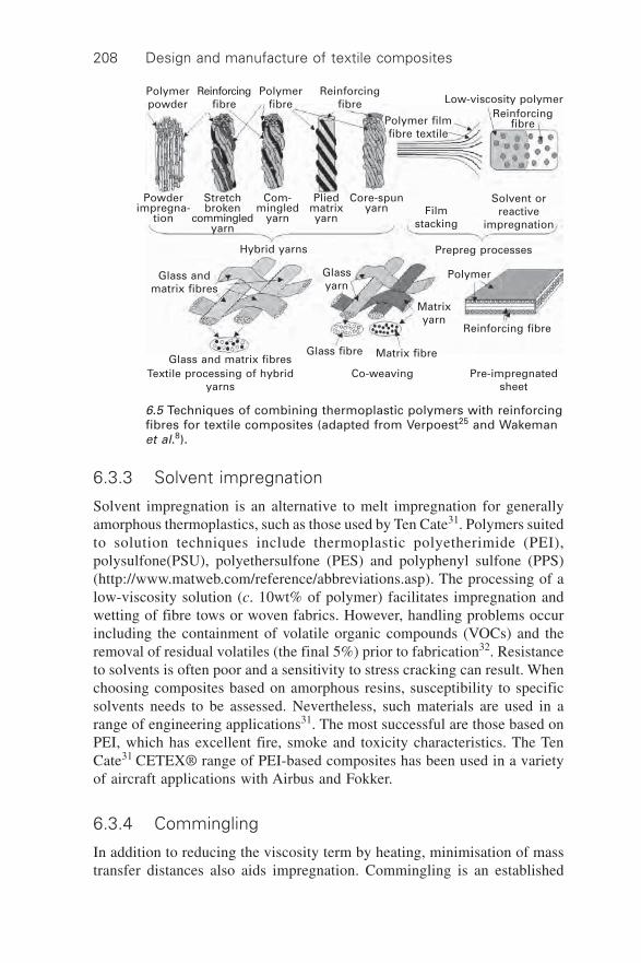
Design and manufacture of textile composites208
6.3.3 Solvent impregnation
Solvent impregnation is an alternative to melt impregnation for generallyamorphous thermoplastics, such as those used by Ten Cate31. Polymers suitedto solution techniques include thermoplastic polyetherimide (PEI),polysulfone(PSU), polyethersulfone (PES) and polyphenyl sulfone (PPS)(http://www.matweb.com/reference/abbreviations.asp). The processing of alow-viscosity solution (c. 10wt% of polymer) facilitates impregnation andwetting of fibre tows or woven fabrics. However, handling problems occurincluding the containment of volatile organic compounds (VOCs) and theremoval of residual volatiles (the final 5%) prior to fabrication32. Resistanceto solvents is often poor and a sensitivity to stress cracking can result. Whenchoosing composites based on amorphous resins, susceptibility to specificsolvents needs to be assessed. Nevertheless, such materials are used in arange of engineering applications31. The most successful are those based onPEI, which has excellent fire, smoke and toxicity characteristics. The TenCate31 CETEX® range of PEI-based composites has been used in a varietyof aircraft applications with Airbus and Fokker.
6.3.4 Commingling
In addition to reducing the viscosity term by heating, minimisation of masstransfer distances also aids impregnation. Commingling is an established
Polymerpowder
Reinforcingfibre
Polymerfibre
Reinforcingfibre
Powderimpregna-
tion
Stretchbroken
commingledyarn
Com-mingled
yarn
Pliedmatrixyarn
Core-spunyarn
Polymer filmfibre textile
Low-viscosity polymerReinforcing
fibre
Filmstacking
Solvent orreactive
impregnation
Prepreg processes
Polymer
Reinforcing fibre
Matrixyarn
Glassyarn
Glass fibre Matrix fibre
Hybrid yarns
Glass andmatrix fibres
Glass and matrix fibresTextile processing of hybrid
yarnsCo-weaving Pre-impregnated
sheet
6.5 Techniques of combining thermoplastic polymers with reinforcingfibres for textile composites (adapted from Verpoest25 and Wakemanet al.8).

Composites manufacturing – thermoplastics 209
Tab
le 6
.2 S
up
plie
rs a
nd
pro
per
ties
of
text
ile t
her
mo
pla
stic
co
mp
osi
te m
ater
ials
Mat
eria
l fo
rmR
ein
forc
emen
tM
atri
xr
s ten
sE
ten
e fai
lure
s fle
xE
flex
ura
l
(g/m
3 )(M
Pa)
(GP
a)%
(MP
a)(G
Pa)
Sa
nd
wic
h m
ate
ria
lM
f%
Qu
adra
nt
GM
Tex
4/1
40G
lass
PP
1220
248
10.5
1.8
280
14.5
GM
Tex
1/1
400–
90∞ g
lass
PP
1200
120
4.9
1.9
160
7.2
(co
mm
ing
led
fab
ric
skin
s,G
MT
co
re)
Exp
erim
enta
lG
F w
eave
4/1
+30
Ran
do
m c
ore
,P
ET
1620
184/
8212
/6.9
1.8/
1.5
––
ran
do
m g
lass
co
refa
bri
c sk
ins
Exp
erim
enta
l75
% w
t 4/
1<7
5P
P f
ilm +
PP
–37
725
–41
021
com
min
gle
dfa
bri
c sk
ins
gla
ss/P
P +
500
:mP
P c
ore
Ali
gn
ed
fib
re m
ate
ria
lsV
f%
Ply
tro
nG
N 6
38T
(m
elt
35[(
0,90
) 2]s
PP
1480
360
162.
530
016
.8im
pre
gn
ated
,su
rfac
e=
0∞ d
irec
tio
n)
GN
638
T (
mel
t35
UD
gla
ssP
P14
8072
0/11
281.
943
621
imp
reg
nat
ed)
tap
e
Tech
tex
tile
sT
her
mo
pre
g35
Sti
tch
ed 0
/90
PP
1700
256
13–
170
–n
on
-cri
mp
fab
ric
inte
rdis
per
edfi
bre
s, G
F
Vet
rote
xTw
inte
x,35
bal
. 2 ¥
2 tw
illP
P14
9030
013
–27
512
com
min
gle
d G
F/P
Pw
eave

Design and manufacture of textile composites210
Tab
le 6
.2 (
Co
nti
nu
ed)
Mat
eria
l fo
rmR
ein
forc
emen
tM
atri
xr
s ten
sE
ten
e fai
lure
s fle
xE
flex
ura
l
(g/m
3 )(M
Pa)
(GP
a)%
(MP
a)(G
Pa)
Vet
rote
xTw
inte
x,35
4/1
wea
veP
P15
0040
024
/8–
380/
160
18/6
com
min
gle
d G
F/P
PTw
inte
x,50
UD
PP
1750
700
38–
400
32co
mm
ing
led
GF/
PP
Twin
tex,
501/
1 w
eave
PE
T19
5044
025
–60
023
com
min
gle
dG
F/P
ET
Twin
tex,
50U
DP
ET
1900
870
37.6
–10
2537
.7co
mm
ing
led
GF/
PE
T
Exp
erim
enta
lG
F/P
ET
48W
arp
kn
itP
ET
–87
/6.6
8.2/
3.5
–74
7/25
35/4
.6G
F/P
BT
560∞
PB
T–
––
–81
040
.5
Po
rch
er I
nd
.P
ow
er52
2/2
twill
PA 1
2–
––
–60
344
imp
reg
nat
ion
carb
on
fab
ric
at f
abri
c le
vel
Ves
top
reg
52B
al.
wea
vePA
12
1850
350/
350
26/2
61.
6/1.
650
022
Co
mfi
lC
om
min
gle
d G
F44
Twill
3/3
PE
T–
260
22–
––
yarn
Co
mm
ing
led
GF
41Tw
ill 3
/3P
ET
–28
020
––
–ya
rn,
mo
dif
ied
PE
T w
ith
lo
wer
Tm
Sch
app
eS
tret
ch b
roke
n56
5HS
car
bo
nPA
12
1440
801
611.
360
652
Tech
niq
ues
com
min
gle
dfa
bri
cfa
bri
c at
20 ∞C

Composites manufacturing – thermoplastics 211
Str
etch
bro
ken
565H
S c
arb
on
PA 1
214
4063
158
1.2
332
42co
mm
ing
led
fab
ric
fab
ric
at 8
0 ∞C
EM
S G
rivo
ryPA
12/c
arb
on
542/
2 tw
illPA
12
1430
790
62.6
1.3
––
(an
ion
ical
lyca
rbo
n f
abri
cp
oly
mer
ised
)
Cyc
lics
Cyc
lic C
BT
–U
D c
arb
on
PB
T16
0015
6511
5–
1310
–
Do
wT
her
mo
pla
stic
–U
D g
lass
ET
PU
1910
1000
452.
211
5045
po
lyu
reth
ane
(76%
Mf)
Bo
nd
TE
PE
X 1
01-g
lass
47G
lass
tw
ill 2
/2PA
66
1800
380
212.
057
022
Lam
inat
esFG
290
(mel
tim
pre
gn
ated
)
TE
PE
X 2
01-c
arb
on
48C
arb
on
tw
ill 2
/2PA
66
1500
755
522.
174
544
C20
0 (m
elt
imp
reg
nat
ed)
BP
Cu
rv (
PP
/PP
–P
oly
pro
pyl
ene
PP
900
180
5–
––
com
po
site
sh
eet)
Gu
rit
SU
Pre
M (
po
wd
er60
Car
bo
n,
UD
PE
EK
–28
0014
21.
920
0012
0im
pre
gn
ated
UD
1 ¥
13 m
m t
ape)
Ten
Cat
eC
ET
EX
PE
I–g
lass
5077
81 g
lass
PE
I19
1046
530
–62
526
fab
ric
CE
TE
X P
EI–
505H
sat
inP
EI
1510
665
56–
830
47ca
rbo
nca
rbo
n f
abri
c
Tab
le 6
.2 (
Co
nti
nu
ed)
Mat
eria
l fo
rmR
ein
forc
emen
tM
atri
xr
s ten
sE
ten
e fai
lure
s fle
xE
flex
ura
l
(g/m
3 )(M
Pa)
(GP
a)%
(MP
a)(G
Pa)

Design and manufacture of textile composites212
Ten
Cat
eC
ET
EX
PP
S–
505H
sat
inP
PS
1550
660
54–
––
carb
on
carb
on
fab
ric
Cyt
ecA
PC
-2 (
mel
t63
UD
car
bo
nP
EE
K–
2400
/82
151/
9.9
–22
8013
8im
pre
gn
ated
)A
S4
carb
on
UD
, u
nid
irec
tio
nal
; G
MTe
x, t
exti
le r
ein
forc
ed g
lass
mat
th
erm
op
last
ic;
500:
m P
P c
ore
, co
re o
f p
oly
pro
pyl
ene
500
mic
rom
eter
s th
ick
Tab
le 6
.2 (
Co
nti
nu
ed)
Mat
eria
l fo
rmR
ein
forc
emen
tM
atri
xr
s ten
sE
ten
e fai
lure
s fle
xE
flex
ura
l
(g/m
3 )(M
Pa)
(GP
a)%
(MP
a)(G
Pa)

Composites manufacturing – thermoplastics 213
textile process for intimately blending reinforcing fibres and matrix in afibrous form. With the short flow lengths given by the hybrid yarn structure,the secondary consolidation and impregnation phases may occur at substantiallylower pressure than those required for conventional melt impregnation. Sincethe hybrid yarns are both flexible and relatively stable, they are suitable forfurther textile processing (e.g. weaving and braiding) and the arising fabricscan be formed conveniently at room temperature. Also, given that the yarnsare (generally) continuous, the reinforcement to matrix ratio can be controlledclosely via the filament size and count of the two yarns. In general, thequality of the laminate is controlled by the intimacy of the blend and theuniformity of the hybrid yarn.
A patented commingling process33, 34 has been developed by Saint-GobainVetrotex for glass and polypropylene yarn (Twintex®). The manufacturingroute consists of drawing and sizing glass fibres (as normal), which are thenpassed to an annular drawing head that is supplied with molten polypropylenefrom an extruder. Under pressure, the molten matrix passes through orificesthat are distributed over an annular die plate and then drawn into multiplecontinuous filaments that converge with the glass fibres to produce commingledyarn at rates of 10–30 m/s. Blowers control air turbulence. Several strategiescan be adopted to maintain yarn integrity including the use of film formersor encapsulants. Where photoactive size is used, the application of ultravioletradiation prior to the winding phase triggers a chemical transformation ofthe size to improve the bonding of the composite yarn. This is especiallyimportant when downstream processes such as braiding are planned, sinceany rewinding operation tends to separate the constituent fibres dependingon their different moduli.
An alternative approach patented by Schappe blends stretch-broken carbonfibres with polyamide 12 (PA12) staple fibres (EMS-GRIVORY, a businessunit of EMS-CHEMIE AG) with the addition of a wrapping filament35,which is available commercially. Multifilaments of reinforcement fibre(typically carbon) are stretch broken by passing yarns through rollers, wherethe roller speed varies between zones, producing a strip of discontinuousfibres of a controllable length (70 mm average). These fibres are thentransformed on standard spinning equipment into the stretch-broken yarn36.The staple matrix fibres and the stretch-broken reinforcement are then broughttogether via a machine having an additional stretching zone that produces aninhomogeneous strip of reinforcing and matrix fibres. Each strip is thencombined with ten other strips on a similar machine and repeated a nominalfour times. The strip obtained is then wrap-spun on a long fibre laminatingsystem before final wrapping of the parallel fibres by a continuous multifilamentof the same matrix as the commingled yarn. This system of yarn productioneliminates the formation of fibres into helices that occurs during conventionaltwisted yarn spinning techniques. A higher degree of mingling is claimed for

Design and manufacture of textile composites214
this process than for competing methods. Additionally, the discontinuousfibres provide additional compliance during forming.
A final approach to commingling37, developed for carbon andpolyetheretherketone (PEEK) systems, involves separating the two yarnsinto open ribbons. The PEEK yarn cannot be opened via an air curtain andis instead passed around polytetrafluoroethene (PTFE) rollers to induce acharge of 6 kV, causing the carbon filaments to repel. The charged bundle isthen drawn into a flat ribbon. The carbon yarn is opened with an air curtaininto a ribbon that is then combined with the PEEK ribbon at a comminglingbar at rates of approximately 0.5 m/s. This, it is suggested, gives a homogeneousdistribution. From the commingling bar, the hybridised fibres are coatedwith size and wrapped on a take-up roll to form the final product. Mechanicalseparating elements that would limit commingling speed are eliminated.
6.3.5 Powder impregnation
The powder-coating approach blends fibres and matrix on an intra-bundlebasis38–40 and is arguably more versatile than commingling in that powdersmay be more readily available than thermoplastic fibres. The process depositsand distributes the powder, most variants of which involve a suspension ofparticles in a fluid stream. The solid particles adhere to the fibres mainly byelectrostatic forces. Success has been reported for fluidised bed processing,aqueous slurries and electrostatic methods of coating. In each case, the yarnsare spread prior to coating to reduce the mass transfer distances. Individualyarns are then passed through an oven to sinter the powder on the fibresurface, creating resin bridges and a semi-impregnated tow that is then fullyimpregnated during the final consolidation stage. An advantage cited forpowder impregnation is the dominant flow direction along the fibre axis thatis in the direction of higher permeability (opposed to flow normal to the fibrewith commingled yarn). Ideally, particles should be at a minimum the samediameter as the fibres, with the consolidation time proportional to the sixthpower of the particle radius. The FIT (fibre-impregnated thermoplastic) process,initially developed by Atochem, impregnated fibre systems with polymerpowder before extruding the same polymer as a sheath around the bundle.The yarn remained sufficiently flexible for textile processing. Commercialproducts40, 41 include unidirectional and cross-ply tapes and broad goods.Fibre contents range typically from 30% to 65%.
An alternative commercial approach involves powder coating unidirectional(UD) tows directly or fabrics after weaving42. In the case of fabrics, they arepassed from rollers in a continuous (e.g. 10 m/min) process under a firstpowder dispenser followed by infrared heaters before a second powder dispenserand a final set of infrared heaters. The material is removed on a take-up rolland fabrics of up to 1000 g/m2 (glass) and 600 g/m2 (carbon) have been

Composites manufacturing – thermoplastics 215
processed successfully at Vf of up to 52% with polymers including PP, PA6,PA12, PPS, PEI and PEEK. Typical particle sizes are 25–100 mm. As withcompeting methods, the coated fabrics may then be consolidated further,laminated alternately, or the initially set product heated in a frame and stampeddirectly.
6.3.6 Co-weaving and warp-knitting techniques
Other techniques, which may be economic in specific circumstances, adaptexisting textile technology and include co-weaving, inter-dispersed fabrics,split-film knits and plied matrix systems25. Co-weaving combines yarns ofthe two fibres into a form possessing good drape characteristics, although anuneven reinforcement to matrix distribution may occur with generally longerimpregnation times compared with a commingled system for a given set ofprocessing parameters. The plied matrix technique43 uses a polymer fibrewoven around a bundle of reinforcement fibres offering improved distributionover the co-weaving technique. Glass and PP yarns have been inter-dispersedon line during fabric formation to produce drapable stitch bonded fabrics44.
Another example is the warp knitting of polymer films with weft insertionof reinforcement fibres45, 46. Split films are cheaper than conventional (spun)polymer fibres and are cut lengthwise into tapes that can be processed in asimilar way to yarns. Weft-insertion warp knitting has been used in this wayto produce multi-axial, non-crimp glass–PET (polyethylene terephthalate)fabrics. Typically, the split films are inserted in the weft, although there is noparticular reason why they could not be warped also. A light stitching yarn(typically PET) provides fabric stability in the usual way. During processing,the textile is restrained during the preheat phase to resist shrinkage of theoriented polymer chains in the stretched ribbon as a return to the random coilorientation occurs.
6.3.7 In-situ polymerisation
An alternative solution is to impregnate the fibre bed using low-viscositymonomers (viscosities in the mPas range) with subsequent in-situpolymerisation that commences with activation of the monomer. Henceimpregnation must occur before the viscosity reaches a limiting level. Whenpolymerisation is complete, depending on the material and time–temperaturetransformation relationship, the part is cooled and the component released.Based on these principles, three main systems based around reaction injectionmoulding (RIM) technology have been adapted to impregnate textile compositestructures via resin transfer moulding (RTM) or pultrusion processes, wheremonomer, activator and initiator systems are injected into a mould wherepolymerisation is completed in a few seconds or minutes, with the

Design and manufacture of textile composites216
polymerisation times generally shorter than for thermoset resin cure cycles47.
Polyurethanes
When mixed, isocyanates and alcohols react to form polyurethanes, whichare found as cross-linked thermoset or linear thermoplastic resins, dependingon the selected molecular chemistry and the polymerisation process48. Dowhas developed thermoplastic polyurethanes for a reactive pultrusion process,known commercially as ‘Fulcrum®’49. Here the thermoplastic polyurethaneresin, which can be repeatedly processed, shows a rapid molecular weightreduction when heated into the processing range. The lower molecular weightmelt also has a low viscosity, enabling impregnation of glass fibres in thepultrusion process. After the impregnation stage, cooling rebuilds the molecularweight to a similar high level as the starting point. Reactive pultrusion linespeeds of 10 m/min have been achieved. Additionally, the urethane chemistryis reported to give good fibre–matrix adhesion. Materials can be recycled viainjection moulding.
Anionic polymerisation of polyamides
Polyamides, denoted by the number of carbon atoms in the monomer unit,can be obtained by the ring-opening polymerisation of lactams50–52, representingmore than 50% of polyamide production. Anionic mechanisms, enabling fastpolymerisation, have been applied commercially (NyRIM) by DSM topolyamide via the RIM technique. This has been used for manufacturingarticles via gravity casting, rotational moulding and RIM, with differentinitiators and activators. This material system has also been used to impregnateglass fibre textile structures in a RTM process, giving a glass fibre PA6composite.
Traditional anionic polymerisation required the combination of two volumesof lactam preblended with catalyst and activator, resulting in a short pot-lifewhere the materials slowly polymerised in the tanks. This was overcomethrough the development of a liquid activator system by EMS Chemie50 thatcontains both activator and catalyst in solution. This has enabled the processingof laurolactam by an anionic ring-opening polymerisation reaction to produceeither a fibre reinforced PA12 part directly53 or a thermoformable pre-preg54, 55.Polymerisation can be completed within minutes, with the type andconcentration of initiator and activator together with the temperature influencingpolymerisation kinetics and the final molecular weight. At 200 ∞C, the viscosityof this material prior to polymerisation is 1 mPa s whereas the molten PA12has a viscosity at this temperature of 50 000 Pa s.

Composites manufacturing – thermoplastics 217
Cyclics technology for PBT, PET and PC
An alternative reactive thermoplastic system is produced by ‘cyclics’technology56. Reinforcement is impregnated with a low-viscosity thermoplasticresin (prepolymer) that subsequently reacts in the presence of heat and acatalyst to increase its molecular weight via conversion of its short molecularchains to a linear structure in a ring-opening polymerisation reaction. Thistechnology has been demonstrated for polybutylene terepthalate (PBT) andpolycarbonate (PC). Two different product forms are available: one-part systemsthat have the resin and catalyst premixed, and two-part systems where theresin and catalyst are supplied separately and mixed during processing. Theprepolymer (CBTTM Resins) starts as a solid at room temperature, melts at150 ∞C to a low viscosity of 150 mPa s, reducing further to below 20 mPa sat 180 ∞C. When mixed with specific tin or titanium catalysts, the PBT ringsin cyclical form open and connect (i.e. polymerise) to form high molecularweight PBT thermoplastic. Full polymerisation is reported to occur fromtens of seconds to many minutes, depending on the temperature and type ofcatalyst used.
6.4 Processing routes
6.4.1 Process windows for textile-based thermoplasticcomposites
A typical processing cycle for a composite with a thermoplastic matrix consistsof heating the constituents above the matrix Tm, applying pressure for a timeperiod to ensure appropriate consolidation, and finally cooling the materialwhile maintaining the pressure. From a manufacturing perspective, consideringequipment investment cost and production rate, it is desirable to process thepart at the lowest pressures and with the shortest cycle times. Reducing cycletimes requires exposing the composite to high heating rates prior to finalshaping and high cooling rates during the solidification stage of the processingcycle.
Optimal processing conditions, in terms of pressure and cooling rate, maybe defined by a processing window (Fig. 6.6)1. The lower cooling rate limitis fixed by economic constraints, since long cycle times are costly. At highcooling rates, a considerable thermal gradient is imposed over the thicknessof the composite part, which leads to both morphological skin–core effectsand thermal skin–core stresses. If the polymer is exposed to excessively hightemperatures during an extended time, thermal degradation mechanisms becomeincreasingly important (and undesirable). Relations between different defectmechanisms, often governed by the internal stress build-up (voiding,microcracking) and cooling rates have been observed. An increased formingpressure, corresponding to the upper right boundary of the diagram, may

Design and manufacture of textile composites218
suppress this defect initiation. The forming pressure upper boundary will begoverned by the practical limit of forces applied by the forming equipment,as well as by the increased tooling cost for high-pressure processes. Highforming pressures may also cause damage to the fibre bed (and changingpermeability) as well as leading to local resin fraction reductions due to ahigh degree of in-plane macro-scale resin flow from the mechanically lockedfibre bed.
Based around these boundary conditions, a wide variety of processingroutes have been developed to process thermoplastic composites. These offerdifferent combinations of cycle time, material suitability (semi-finished productssuch as partially impregnated sheets or as textile structures composed of, forexample, commingled yarns) and the investment in capital equipment needed.
6.4.2 Low-pressure processing techniques
A range of low-pressure processing techniques have been developed thatrely on the intimate fibre and matrix distribution before processing, either ina ‘dry’ commingled yarn material, or a preconsolidated laminate. The lowerpressures reduce the investment in tooling and forming equipment, which isan important consideration for lower manufacturing volumes.
Vacuum forming of thermoplastic composites
Thermoplastic composites can be processed by vacuum forming in a similarmanner to thermoset composites. Vacuum forming also enables thermoplastic
Pre
ssu
re
Eco
no
mic
lim
itat
ion
sT
her
mal
deg
rad
atio
n
Morphological skin–core effectsThermal skin–core stresses
Res
tric
ted
flo
wP
ract
ical
lim
itat
ion
s
Optimalprocessing
region
Equipment limitations
Uncontrolled flow
Fibre damage
Resin starvation
Cooling rate, log (dT/dt)
6.6 Generic process window for thermoplastic textile composites(adapted from Månson et al.1). T = temperature, t = time.

Composites manufacturing – thermoplastics 219
composites to be used in a hand lay-up type process. The produced part hasonly one surface with a finish that reflects the surface of the mould. Cycletimes are a function of the heating route and sample size, ranging from 60 s57
for carbon fibre (CF) reinforced PEEK, to 15 mins for glass fibre (GF)/PPplates58 and to 24 h for a 7 m rigid inflatable boat59. With a two-shift pattern,a typical production volume is 30 parts per day60.
Taking the example of commingled yarn-based textiles, the first processstep is to position the material into a mould. Techniques employed to hold‘dry’ commingled fabrics to vertical mould walls and to subsequent layersinclude the use of hot air guns to ‘tack’ layers together and, for polypropylene-based materials, a pressure-sensitive polypropylene-based adhesive that isfabric coated onto the commingled textile, together with low molecular weightpolyolefin spray contact adhesives (e.g. 3M-77). Core materials, which resistcollapse at the composite process temperature and pressure, can also beincorporated, with typical materials including foams (e.g. Airex KapexC51),aluminium honeycomb and balsa wood. Release agents are often used tofacilitate part release.
For well-consolidated parts (low porosity), a perforated peel ply (100 g/m2) and breather felt (non-woven nylon or nylon-PET of 100–300 g/m2) areused beneath the vacuum bag, which enables the air to be fully evacuated.The peel ply is in direct contact with the thermoplastic composite to preventadhesion between the breather felt and the moulded material. The vacuumbag can consist of several materials, which for the case of polypropylene-based composites must have a melting temperature above 200 ∞C. Dependingupon production volumes, a flexible nylon vacuum bag (50–75 mm) or a pre-shaped reusable silicone rubber bag is sealed against the surface of the tool.Reusable silicon membranes can be used to replace films, reducing consumablecosts and the time needed to position the vacuum system. Typically only100–150 parts total production volume are needed to offset the higher initialcosts. Preformed silicon rubber forms enable a male tool to be used.
With a vacuum approaching 1 bar being applied for the whole processingcycle, the tool and material are heated under vacuum to the polymer’s processingtemperature (e.g. 185–190∞ C for PP), which is maintained for typically 10–20 min (dependent on the textile fibre and matrix distribution) for fullimpregnation. The tool is then cooled to below 70 ∞C (to reduce distortionand ease handling) with the vacuum pressure still applied, after which thevacuum bag is removed and the part released.
As this is an isothermal process where the mould temperature is cycledabove and below the composite matrix Tm, the overall mould mass that isheated and cooled needs to be minimised. The mould material chosen dependson the number of parts to be produced, the cycle time desired, and thesurface finish needed. Four general types of mould are used: high-temperatureepoxy composite (3000–6000 parts/mould), welded metal sheet moulds (5000–

Design and manufacture of textile composites220
10 000 parts/mould), cast or machined aluminium (10 000–30 000 parts/mould) and electroformed nickel shell (50 000–100 000 parts/mould)60.
Several methods are available to heat the evacuated tool depending on thesize of the part, with the important requirement of a homogeneous temperaturedistribution. Heated tools avoid the need for a heated enclosure but are part-specific and generally used for part areas of 1–3 m2 (Fig. 6.7a). However,tool durability is reduced due to differential expansion between the differentmould materials and heating systems. Ovens offer a clean heating route,enabling a variety of components, including large structures, to be madefrom one heating system (Fig. 6.7b).
Vacuum moulded part
Oven Vacuumsystem
Frame structure
Tool (e.g. weldedmetal sheet)
(b) Heating via oven(a) Heated tools (e.g. 20 ∞C to190 ∞C to 20 ∞C for PP)
Frame structure
Tool(e.g. glass/epoxy) with
heating/coolingcircuits
Thermoplasticcompositematerial
SealantVacuumConnectorVacuum bag
Non-wovenbreather felt
Perforatedpeel ply
6.7 Vacuum bag processing of thermoplastic composites.
As an example of the vacuum moulding process, a rigid inflatable boathull59 has been produced from commingled glass and PP textiles. A mouldmaterial was needed that would withstand 500 production cycles. The contouredbase is a cast mould equipped with heating and cooling systems. The textureand colour of the component can be changed using thermoplastic films thatare placed on the mould surface. For such a production volume, neithermetal nor nickel-shell tooling was cost effective and hence composite toolingwas developed using a high-temperature divinylmethane diisocyanate toolingresin. This produces a high-quality gel coat surface and can be highly filledwith metallic powder to improve the thermal conductivity. Where appropriate,a heating system can be integrated into the mould by either laminating inPTFE-coated resistance wires (e.g. 2500 W/m2) or copper tubes for hot oil.

Composites manufacturing – thermoplastics 221
In the case of the electrically heated mould, the resistance wires are fabricatedinto a grid that is draped just beneath the mould surface. Using an oil heatingsystem, 40 min were required to heat commingled fabric across the boatstructure to melt temperature. Pressure was applied for a further 40 minbefore the cooling cycle of 20 min where cold water was passed through theintegrated copper tubes, giving a total process cycle time of approximately100 min. This was reduced to 45 min for the electrically heated mould.
Autoclave forming of thermoplastic composites
In an extension of the vacuum moulding process, autoclaves offer similaradvantages to ovens during the heating stage (heating of the assembled mould,textile composite and vacuum bag) with the ability to apply additional externalpressure from 3.5 to 7 bar. This reduces void content and offers closer thicknesstolerances, but reduces the number of parts made per day (Fig. 6.8)61. Formingis performed by raising the autoclave temperature to above the matrix Tm
followed by an increase of the autoclave pressure to effect forming andfinally cooling under consolidation pressure. During forming, the mould issubjected to hydrostatic pressure and the only force tending to distort themould is the reaction to the diaphragm stretching, which in the case ofpolymeric diaphragms is very low. Thin section moulds with low thermalmass can be used.
6.8 Autoclave processing (double diaphragm forming) ofthermoplastic composites (adapted from Mallon et al.61).
Compressednitrogensupply
Heated pressure vessel
Composite laminate Top diaphragm
P+
P–
Moulded part
Bottom diaphragmMouldVacuum
Diaphragm forming
Diaphragm forming is a technique that consists of placing the laminate betweentwo thin plastically deformable sheets, known as diaphragms. The diaphragms,when clamped around the mould edge, maintain biaxial tension on the laminate

Design and manufacture of textile composites222
during deformation, consequently restricting laminate wrinkling, splittingand thin spots. The normal procedure consists of heating the whole mould,laminate and diaphragms to above the laminate polymer Tm, generally limitingprocess cycle times to 30 min or more. The combination of air pressureabove the diaphragm, and a vacuum drawn from beneath the diaphragmforces the laminate to the mould geometry enabling the production of complexparts. Diaphragm forming can be performed either using compressed air oran autoclave. As an alternative to using two diaphragms, a single diaphragmplaced over the preform can effect forming in a similar manner to doublediaphragm forming (Fig. 6.9).
Upperdiaphragm Clamping pressure
Heatedcomposite
Pressure
Cool/hot tool Vacuum
Moulded part
6.9 Isothermal single diaphragm forming of thermoplasticcomposites.
The diaphragms most commonly used are either polymeric or metallic62.Metallic diaphragms, such as superplastic aluminium, have been used forforming APC-2 (CF/PEEK) laminates. Polyimide films, such as Upilex-R(0.13 mm thick), have good elongation properties at temperatures up to400 ∞C and have been used extensively. During forming, the laminate canslide within the diaphragms. As the diaphragms are stretched, surface frictionbetween the laminate and the diaphragms transmits tensile forces to thelaminate, creating out-of-plane support and suppressing wrinkling.
Recent developments have applied this technique to commingled glassand polypropylene textiles where panels have been produced using 0.5–1.0mm thick silicone sheets. The composite fabrics and two silicon sheets arepreheated in an initial stage between hot platens (210 ∞C) before rapid transferto the forming unit and the application of positive pressure (7 bar) to formthe material into a ‘female’ tool (Fig. 6.10). The silicon membranes arereusable, for between 500 and 1000 parts in polypropylene. This reducescycle times to typically 2 min, as the temperature of the one-sided moulddoes not need to be thermally cycled.

Composites manufacturing – thermoplastics 223
Bladder inflation moulding
The bladder inflation moulding (BIM) technique enables production ofcomposite components with hollow geometries that have both high geometricalcomplexity and high intrinsic stiffness63–66. BIM uses an outer mould andinner bladder to define the shape of the part. The low process pressures (~10bar) permit the use of simple tooling, giving a process for producing thin-walled hollow composite parts with evolving cross-sections. Previous workhas demonstrated bladder inflation moulding for small generic components,bicycle frames and handlebars, tennis rackets, suspension arms and pressurevessels65. Two process variants of the BIM technique have been developed:(i) an isothermal process where the mould temperature and thereby thecomposite temperature is cycled above and below the composite matrix Tm
(Fig. 6.11) and (ii) a non-isothermal process where the thermoplastic compositetextile is preheated above the matrix Tm outside of the mould and thentransferred rapidly to the cool mould for bladder moulding (Fig. 6.12).
Contact pressure Heatedcomposite
Rapidtransfer
Clampingpressure
Clampingpressure
Pressure
Moulded partVacuumWarm toolUpper &lower
diaphragms
Heated plates
6.10 Non-isothermal double diaphragm forming of thermoplasticcomposites – external heating in hot plates and rapid transfer.
Compositematerial
Coolmould
Compositematerial
Heat source
Clamping force
Cooling methodCool mould
BladderCooling method
Internalpressure
Hotmould
Heat source
BladderBladder
(a) Materials (b) Assemblebladder &compositein mould
(c) Heat mouldsufficiently(above matrix Tm)maintain pressure
(d) Cool mouldsufficiently(below matrix Tm)maintain pressure
(e) Final part
6.11 A cross-sectional sequential view of the isothermal bladderinflation moulding process.
The isothermal BIM (isoBIM) process (Fig. 6.11) consists of assemblinga thermoplastic composite braid around a bladder, which is pressurised
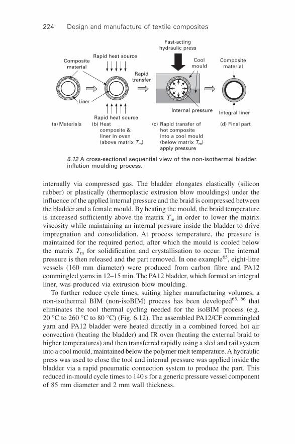
Design and manufacture of textile composites224
internally via compressed gas. The bladder elongates elastically (siliconrubber) or plastically (thermoplastic extrusion blow mouldings) under theinfluence of the applied internal pressure and the braid is compressed betweenthe bladder and a female mould. By heating the mould, the braid temperatureis increased sufficiently above the matrix Tm in order to lower the matrixviscosity while maintaining an internal pressure inside the bladder to driveimpregnation and consolidation. At process temperature, the pressure ismaintained for the required period, after which the mould is cooled belowthe matrix Tm for solidification and crystallisation to occur. The internalpressure is then released and the part removed. In one example65, eight-litrevessels (160 mm diameter) were produced from carbon fibre and PA12commingled yarns in 12–15 min. The PA12 bladder, which formed an integralliner, was produced via extrusion blow-moulding.
To further reduce cycle times, suiting higher manufacturing volumes, anon-isothermal BIM (non-isoBIM) process has been developed65, 66 thateliminates the tool thermal cycling needed for the isoBIM process (e.g.20 ∞C to 260 ∞C to 80 ∞C) (Fig. 6.12). The assembled PA12/CF commingledyarn and PA12 bladder were heated directly in a combined forced hot airconvection (heating the bladder) and IR oven (heating the external braid tohigher temperatures) and then transferred rapidly using a sled and rail systeminto a cool mould, maintained below the polymer melt temperature. A hydraulicpress was used to close the tool and internal pressure was applied inside thebladder via a rapid pneumatic connection system to produce the part. Thisreduced in-mould cycle times to 140 s for a generic pressure vessel componentof 85 mm diameter and 2 mm wall thickness.
Compositematerial
Coolmould
Rapidtransfer
Rapid heat source
Fast-actinghydraulic press
Compositematerial
Liner
Rapid heat sourceInternal pressure Integral liner
(a) Materials (b) Heat (c) Rapid transfer of (d) Final partcomposite & hot compositeliner in oven into a cool mould(above matrix Tm) (below matrix Tm)
apply pressure
6.12 A cross-sectional sequential view of the non-isothermal bladderinflation moulding process.

Composites manufacturing – thermoplastics 225
Reactive thermoplastic RTM
RTM techniques that are commonly used for thermosetting resins are alsoapplicable to reactive thermoplastic resins. Thermoplastic RTM (TP-RTM)has been used to produce both generic plates54, 55 and sections of a car floorpan53. As an example, TP-RTM of a PA12 material consisted of the followingsteps, which are shown schematically in Fig. 6.13. The injection unit consistsof two tanks, two gear pumps and two pipes conveying respectively theactivator and the monomer from the tanks to the mixing head. The monomeris in the molten state; therefore tank, pump and pipes are maintained at180 ∞C during processing. The liquid system remains at room temperature toavoid degradation. Both materials need to be held under nitrogen. Immediatelyprior to injection, mixing of the molten monomer and the liquid activatorsystem (2.5%) occurs in a static mixing head.
N2
Toil
Tmonomer
Tbox
HeaterPump Valve
Those monomer
Tmix
Mixing head
Valve
Clampingforce
Upper tool
Lower tool
InsulationMould heating &cooling conduits
(above and belowmatrix Tm)
Activated monomer/polymerising material
flow front throughfibre bed
Thicknesschanges, ribs/
stiffeners,complex features
Injection point
Final part
N2
ReactiveinjectionmachineValve
Pump
N2
Tliquid system
Toil = 170 ∞CTmonomer = 165 ∞CTliquid system = 20 ∞CThose = 200 ∞C monomer
Tmix = 180 ∞CTbox = 200 ∞CPmax = 10 barVliquid system = 2 dm3
Vmonomer = 25 dm3
6.13 Reactive thermoplastic RTM process, with the reactive injectionmachine illustrated for APLC12 materials (PA12 final polymer).
This particular monomer and activator system requires isothermal processingfor economic processing. The mould temperature needs to be cycled fromabove the monomer Tm of 150 ∞C to a peak ranging from 200 ∞C to 250 ∞C(with higher temperatures increasing the polymerisation rate), followed bycooling sufficiently below the PA12 polymer Tm of 175 ∞C for demoulding.

Design and manufacture of textile composites226
An aluminium mould was used that enabled the production and study of 450mm ¥ 550 mm plates of 1–3 mm thickness. Using oil heating, less than 30min was required to reach a mould temperature of 200 ∞C, and with watercooling, temperatures were reduced from 200 ∞C to 50 ∞C in 5 min.
The TP–RTM cycle consisted of the following steps. First, a release agentcompatible with the anionic polymerisation was applied to the mould andtwo layers of a dried 5-harness satin carbon weave (440 g/m2) laid in themould cavity [0/90]s. Nitrogen was then flushed through the closed mould toremove oxygen and residual moisture. As the mould temperature exceeded180 ∞C, activated monomer was injected into the mould. When the mouldcavity was full with polymerising material, inlets and outlets were closedand heating maintained to enable complete polymerisation. The polymerisedmaterial then solidified during cooling, before final demoulding. The wholeprocessing cycle required less than 60 min, with this being reduced to 15 minfor a tool with faster heating circuits. This process has been used to producea section of an automotive floor pan structure, offering the advantages ofincreased toughness and the ability to post form materials53.
Injection-compression techniques have also been used to controlcrystallisation-based shrinkage and associated void formation to reduce porositylevels from 10% to 1%. Injection-compression processing applies a typicalsurface pressure of 55 bar during the cooling phase, using a shear edgetool.
The polymerisation of cyclic butylene terephthalate oligomers to form aPBT material system (offered by Cyclics56) is also suited to TP-RTM. Theprepolymers can be processed without cycling the mould temperature andwill melt, polymerise and solidify when processed between 180 and 200 ∞C.With a prepolymer melting point of 150 ∞C, a processing temperature (mouldtemperature) of 180–190 ∞C is reported to give a compromise between higherrates of polymerisation and crystallisation. As the polymerised PBT has amelt temperature of 220 ∞C, the mould does not need to be cooled before partrelease. Cyclics® Corporation56 claims to have demonstrated the use ofCBTTM resins in the following textile composite processes: compressionmoulding, vacuum bagging, resin film infusion (RFI), RIM structural reactioninjection moulding (SRIM), RTM and pultrusion.
6.4.3 High-pressure processing
Press-based processes, often involving separate preheating of the compositeand then moulding in a cool tool, require higher forming pressures due to theshort residence time in the tool under pressure during which final impregnationand consolidation need to occur. These processes have evolved to reducecosts and decrease cycle times for high-volume manufacturing. The alternative(isothermal) technique of cycling the tool temperature is less suited to high

Composites manufacturing – thermoplastics 227
production volumes, requiring large transfers of energy and resulting ingenerally longer cycle times and higher operating costs.
During non-isothermal processing, drapable textiles are still essential formaximum formability, but there is no longer a need for the composite productto have tack or drape at room temperature (forming occurs above matrix Tm),and a degree of mechanical handling integrity is desirable. The choice offully impregnated, partially impregnated or unconsolidated material forms isan interaction of economics (eliminating pre-consolidation costs vs. potentiallylower stamping times) and mechanical properties (cycle time vs. void content)and of practical handling considerations (degree of automation). Pre-consolidation eliminates the need to heat multiple layers of fabric, whichmust be assembled before stamping. Where fully pre-consolidated materialsare used, the final stamping stage forces the material to conform to themould geometry and (ideally) to eliminate any deconsolidation introducedduring preheating. A comparison of stamp-forming with unconsolidated (drycommingled textile), partially pre-consolidated (40% porosity) and fully pre-consolidated CF/PA12 commingled yarn material showed increased laminateproperties and reduced porosities for increasing levels of pre-consolidation,with the effect strongest at lower forming temperatures54.
The following processing techniques, described after a brief examinationof common preheating and blank holder technologies, are essentially allstamp-forming variants. After heating of the material to processing temperature,the primary forming mechanisms are the simultaneous phases of9 intra-plyshearing to facilitate fabric deformation, inter-ply shearing for shapeaccommodation (for two or more plies), viscous-friction between the pliesand tool surfaces, pressure application for consolidation and removal of heatto permit solidification of the matrix.
Preheating technology for stamp-forming processes
Established industrial preheating techniques include infrared, hot air and airimpingement heating, with contact heating, microwave, radio frequency andresistance heating (for carbon materials) under development67–69. Infraredheating70 offers several advantages, including fast absorber heat-up times,programmable heating, controllability and higher energy efficiency. Problemsoccur with surface and through-thickness temperature inhomogeneities, whichare oven design issues71. Circulated hot air ovens72 are best used for porousmaterials or pre-consolidated sheets that strongly deconsolidate. They havelonger response times compared with infrared, but limit degradation fromhigh flux levels at the composite surface and generally give a more evensurface temperature distribution. Additionally, inert gases can be used tofurther reduce degradation. Air impingement ovens direct hot air at highvelocity towards the composite blank and limit the upper temperature.

Design and manufacture of textile composites228
Infrared oven emitters radiate electromagnetic energy in the infrared region,with the laminate reflecting, absorbing or transmitting this energy. Heattransfer occurs when radiation is absorbed, increasing the random molecularenergy. For example, carbon black pigmented PP shows minimal transmission,with 3% reflection and 97% absorption, irrespective of the wavelength, overthe range of 0.8–3 mm73. This analysis needs to be performed for the specificpolymer in question. Therefore, only as much energy can be delivered to thesurface as can be transferred into the blank, without the surface overheating.The advantages of short wave emitters for PP are therefore limited to reducingresponse times and hence increasing the control potential.
A preheat processing window (Fig. 6.14) can be established as a periodwhere the mid-plane of the laminate has reached the desired processingtemperature for impregnation but without degradation at the outer surfaces.Different textile composite forms exhibit different heat transfer characteristics,for example, the range of pre-consolidation levels between a ‘dry’ commingledtextile and a fully pre-impregnated laminate. Additionally, fully impregnatedmaterials (fibre architecture dependent) will deconsolidate during heating74
due to release of strain energy in the reinforcing fibres, the condensation ofdissolved gas into voids of finite size17 and fibre to matrix adhesion effects.Hence during heating, the centre of the composite can become insulatedbecause of its lofted structure. High matrix viscosities require heating to themaximum temperature possible to facilitate impregnation, while avoidingoxidative degradation, which results in chain scission of the macromolecules,and hence a reduction in the molecular weight. Matrix degradation occurs asa function of both temperature and time at temperature and frequently phosphite
6.14 Example of a preheat window for PP-based thermoplasticcomposites.
Tem
per
atu
re (∞C
)
250
225
200
175
150
125
100
75
50
25
0
Oven temp.
Middle
Degradation
Processingwindow
(199–227 ∞C)Top
Bottom
Cooling
0 60 120 180 240 300 360 420 480 540Time (s)

Composites manufacturing – thermoplastics 229
antioxidants are used75 to minimise these effects during both preheating andthe service life of subsequent products. As an example, gel permeationchromatography (GPC) has been used to define the upper processing windowlimit (with a given stabiliser package) for glass and PP laminates73. Higherlaminate temperatures reduced the time to the onset of degradation. For astandard infrared oven and for a laminate temperature of 220 ∞C, the preheattime adopted for the fabric blank of 145 s was within the onset of degradationat 200 s. At laminate temperatures of 180 ∞C, preheat times of greater than10 min were possible.
Engineering polymers, such as PEI, require pre-drying before the mainheating cycle, for example 4 h at 150 ∞C, to remove residual moisture. Thisis not necessary for commodity polymers such as PP.
Blank-holders and membrane forces
Blank-holders are a common feature of the stamp-forming processes discussedbelow, performing three principal functions. Due to thermoplastic memoryeffects, the matrix phase of certain composite textiles shrinks during preheating,requiring a blank-holder to hold the material. Additionally, to maintain fibreorientations correctly in the final part, an automated route is needed to transferthe hot and hence conformable material from the oven to the tool. Manualtransfer is unsuitable because of the rapid convective heat loss and alsolocalised conductive heat loss where the operator grips the laminate. Blank-holders thus restrain the material during preheating and also enable rapid(<10 s) transfer to the cool mould, which has been minimised in practice to2–3 s10, 29.
To maximise fabric drapability and reduce forming faults during moulding,a membrane stress should be applied to the fabric by a blank-holder, permittinghigher shearing angles without visible wrinkling. For example, a 20 MPamembrane stress increased fabric shear angles from 35∞ to 60∞ without visiblewrinkling10. As the fabric conforms to the tool, it is pulled through the blank-holder when the force needed to overcome the viscous friction at the fabric/blank-holder contact interface is less than the force needed to continue intra-ply shearing. The clamping load is transmitted to the fibre through the shearaction of the resin, which will act as a lubricant depending on matrixtemperature. Resistance at the tool/ply and ply/blank-holder interfaces is afunction of the matrix film viscosity and Coulomb friction from the reinforcingfibre and tool contact. Increased pullout velocities and normal pressuresincrease the shear stress. Blank-holder temperatures should be lower thanthe material bulk76; for PP-based composites, a blank-holder temperature of125 ∞C improved quality versus 50 ∞C. An alternative to planar blank-holdersis to clamp the fabric between rollers at selected zones, with the knurledroller surface fixing but not damaging the sheets10. The torque resistance of

Design and manufacture of textile composites230
the rollers inhibits draw-in of the material into the mould, with the normalpressure on the rollers controlled via pneumatic cylinders to vary retainingforces as a function of draw depth. This reduces heat transfer from the hotsheet to the blank-holder by the small contact surface of the rollers, reducingresidual stresses where high membrane tensions are used.
Elastomeric tool forming
The upper tool used in this process consists of an elastomeric pad that can becontoured to match the shape of the lower mould for forming complex shapedcomponents (Fig. 6.15). Elastomeric moulds deform elastically to a rigidlower mould under relatively low loading, but with low compressibility(constant volume). In the locked situation, elastomeric tools behave nearhydrostatically, where an increase in the applied force on the mould transmitsto a general increase in surface pressure on the whole laminate. Consolidationquality is influenced less by the part geometry than where two rigid mouldsare used. Rubber moulds can be created from polyurethane or cast siliconrubber types (e.g. GE RTV630, offering high strength and tear resistancewith inherent release capabilities). The laminate is preheated to above thematrix Tm and transferred rapidly into the mould. Blank-holders are used tocontrol wrinkling. Closing of the mould deforms the laminate into the requiredshape and subsequently the component cools and solidifies within the mould.Marginally longer cycle times are needed than for matched metal mouldsbecause of the lower thermal conductivity of the rubber mould. By changingthe rubber tool geometry, the pressure distribution around the mould can bevaried. The flexible nature of the mould accommodates composite materialthickness variations caused by deformation of the laminate during forming.
Accumulators
Moving bolster
Rigid lower tool
Fast-acting hydraulicpress
Formed part
Blank-holderto apply
membranestresses
Textile sheetfor forming
Infrared oven
EmittersReflectors
Transferframe
Controlpyrometers
Heatedcomposite
Rapidtransferdevice
Shapedrubber tool
6.15 Use of shaped elastomeric tooling for the stamping–forming oftextile composites.

Composites manufacturing – thermoplastics 231
Elastomeric moulds are generally less suited to very high production volumesdue to the reduced tool life compared with metallic moulds (contact with hotlaminates and a low rubber thermal conductivity)12.
The rubber pad may also be in the form of a rubber block (Fig. 6.16). Thisis generally suited to forming only simple shaped components, due to thelimited local deformation of the rubber pad. Rubber block pressing provideshigh normal forces and surface tension but these are not uniformly distributedover the laminate. The local forming forces are determined by the shape ofthe die only, which counteracts closure of the press. Such processes havebeen widely used in production for Airbus and Fokker aerospace applications,in PEI and PPS-based textile composites (CETEX®).
6.16 Deformable rubber block tooling for the stamping–forming oftextile composites.
Rubberblock
Pressure
Infraredoven
Rigid lower tool
Formed part
Hydroforming
The hydroforming process (Fig. 6.17) utilises fluid pressure (hydraulic oil)behind a rubber diaphragm to force a sheet of material into the shape of anadjoining mould. The cut textile preform is first located on the diaphragmthat is fixed to the fluid filled chamber. The draw-cap is fixed in position andthe punch lowered to form the part against the resistance of the fluid pressure.Both the punch and the fluid are held at the appropriate temperature and,after the required hold time, the pressure is released, the punch withdrawnand the part removed. The main advantage of hydroforming is the applicationof hydrostatic pressure and a uniform normal pressure over the laminatesurface, during both forming and consolidation phases. This facilitates thedeformation mechanisms of inter-ply and intra-ply shear while at the sametime squeeze flow effects are not restricted. As a result, the formed part willnot suffer from damage in high spots and sharp corners in the same way ascan occur in matched die forming.
Hydroforming, like diaphragm forming, eliminates the need for mutuallyconforming dies and consequently the tooling costs are relatively low.Elastomers used in hydroforming are generally suited only to lowertemperatures and hence, for higher temperatures, additional rubber sheets

Design and manufacture of textile composites232
have been placed over the preform before forming to prevent diaphragmrupture. Compared with diaphragm forming, hydroforming offers fewerpossibilities to control forming forces on the laminate, but higher hydrostaticpressures can be imposed on the laminate surface.
Rapid stamp-forming with matched rigid moulds
The rapid stamping technique (Fig. 6.18) has been extended from moretraditional techniques such as diaphragm forming for high-volume or cost-sensitive industrial sectors, notably the automotive industry. Metallic toolsare necessary to achieve the high heat transfer rates needed to reduce cycletimes. The process consists of preheating the textile in an oven to above thematrix Tm before rapid transfer to a cool tool where forming and consolidationtake place. Blank-holders are used to control wrinkling. With considerationof the following issues, textile composites can be processed with matchedmetal tools using the techniques commonly used for GMTs:
∑ avoid obstructing deformation of the laminate when local pressure isapplied too early;
∑ thickness differences due to intraply shearing must be predicted precisely(dependent on the fabric type and the initial orientation in the tool);
∑ the final consolidation will be different over the product due to differentsurface pressures during the consolidation phase (e.g. wall sections withlower normal pressures);
∑ fabric waste management and recycling.
Rigid upper toolFlexible
diaphragm
Pressure
Rigid upper tool
Formed partPressurisedOil
reservoir
Infraredoven
6.17 Hydroforming of textile composites.
Preheated sheet
Blank-holder
Trimming
Constantthickness
Formed part
6.18 Non-isothermal stamping of thermoplastic textile composites.

Composites manufacturing – thermoplastics 233
The required consolidation pressure depends on the tolerated porositylevel, but 5–15 bar is typical3, 29, and pressures above 40 bar (e.g. for GF/PPand CF/PEI) may promote resin percolation to the outer plies9, 77. The formingrate has important effects during processing. Reported stamping rates include25 and 210 mm/s for PP and PPS systems78, and 12 to 166 mm/s for glass orcarbon and PA1210, 54. Higher stamping rates reduce material cooling andwere found to increase hemisphere quality for CF/PA12 materials. Examinationof four materials at rates of 10–100 mm/s, with right angle and cylindricaldish tools, showed that higher forming rates limited inter-ply slip, resultingin increased surface fibre buckling79. The use of a rapid approach, followedby a relatively slow forming and consolidation period, has also been suggested.Mould temperatures are material (matrix) dependent and are recommendedas: 80 ∞C (PP), 130–160 ∞C (PA), >160 ∞C (PPS), 230–280 ∞C (PEI) and230–300 ∞C (PEEK). Cool moulds cause matrix solidification prior to completepart drape (limiting inter-ply slip) whereas materials conform fully at higherforming rates with warmer tools.
Continuous compression moulding
This is a derivative of the stamp-forming process where materials are fedinto a preheat oven and then into an intermittent press with a heating andcooling zone80. The process is normally automated. The material is pulledthrough the tool when the press is open and feed stops as the section ofmaterial in the tool is compressed. The tool then opens again and the materialis advanced, by a step size smaller than the part size. Shaped flat sections,‘U’ sections, ‘I’ sections and ‘II’ sections can be produced together withclosed hollow sections. Shapes with a constant radius (in one degree offreedom only) can also be formed. The lay-up of the composite sheet used tofeed the process can be varied, such that UD fibres can be located on theflange area, and ±45∞ fibres on the wall areas of an ‘I’ beam. Pressures of 25bar are typically applied, and feed rates of 30–80 m/h are common. Partthickness of 5 mm is possible and 30 mm thick sandwich structures can bemade. The process is shown schematically in Fig. 6.19.
6.5 Novel thermoplastic composite
manufacturing routes
6.5.1 Co-compression moulding of textile preformswith a flowable core
In addition to adding thickness changes and functional parts (ribs and bosses)to a structural item, the compression moulding of fabrics is often madeeasier by incorporating compliant polymer film or GMT interleaves between

Design and manufacture of textile composites234
layers of fabric to overcome problems of thickness variations and areas ofpoor consolidation (Fig. 6.20)13,14. While the flow-moulding core can reducethe overall Vf, it has a minimal effect on flexural stiffness. The polymer orfibre suspension flows in an open channel at the inter-ply region (insulatedfrom the relatively cold tool by the outer plies), yielding pseudo-hydrostaticconsolidation. This has been demonstrated14 for an automotive door module,producing a fourfold increase in modulus over monolithic GMT, with nocycle time penalty. An example of a material commercially available fromBond Laminates27, 28 is ‘flow-core’ and Quadrant GMTex® where commingledfabric skins have been combined in a double belt press with a GMT core,which are now in series production for automotive applications. Another
6.19 Continuous compression moulding for the stamping–forming oftextile composites.
±45∞ OO
Textile sheetfor forming
EmittersReflectors Hot lower tool
Cool lower toolFormed part(continuous)
Advance+ post-treatment
Cool uppertool
Accumulators
Hot upper tool
Infrared oven Intermittent fast-actinghydraulic press
Moving bolster
Fabric
GMT orpolymer film
GMT/film
Commingled fabric:glass & PP
6.20 Co-compression moulding of textile composites with acompliant core.

Composites manufacturing – thermoplastics 235
solution is the extrusion of long fibre thermoplastics (LFTs) betweencommingled fabric skins prior to compression moulding81. This co-compressionmoulding technique gives a solution for applications that do not need textilereinforcement to the edge of the component, where the area of aligned fibrematerials is smaller than the tool, eliminating waste and the need forblankholders during preheat and transfer stages. This has also been appliedto more conventional sandwich structures using either polymeric foam orhoneycomb cores81.
6.5.2 Over-injection moulding of stamped preforms
A hybrid moulding process, developed by EPFL-LTC83–85, that enablescomposite stampings to be over-injection moulded (by direct recycling ofwaste prepreg material) is shown in Fig. 6.21. The combination of sheetstamping with over-injection moulding facilitates the combination of theintrinsic stiffness of sheet forming with the ability to include a high degreeof integrated functionality via the over-injected polymer. The key issue behindthe process is to achieve interfacial healing between the hot, over-mouldedpolymer and the warm textile composite stamping, with the requirement thatthe average temperature of the two is above the polymer Tm
86–88. In practice,a standard injection moulding tool and melt temperatures (e.g. 50 ∞C and 240
6.21 Over-injection moulding of stamped textile composites:(a) rectilinear stamped sheet and (b) net-shape stamped sheet.
Bosses &complexfeatures
Bosses &complexfeatures
Sealingchannels
Ribs &stiffeners
Local structural insert
Ribs &stiffeners
Sealingchannels Structural insert to
edge of part
(a)
(b)
Infrared heaters
Fabric
(1) Preheat fabric (2) Stamp fabric (3) Over-inject complex features
Female mould
Injectedpolymer
Over-injection toolStamping tools
Local structural insert
Trimmedstamping
Structural insertto edge of part
Scrap(over-injected)
Stamped composite sheet Over-moulded stamped sheet

Design and manufacture of textile composites236
∞C respectively for PP) can be used where the stamped insert is preheatedoff-line to a temperature below the polymer Tm (e.g. 150 ∞C for PP). Thismaintains the rigidity of the insert during transfer into the over-mouldingtool and also gives the thermal requirements needed for in-situ fusion bonding.Ejector pins can be used to hold the sheet in position while the injectionmoulding tool fills. The pins are removed when the tool is full but beforepacking pressure is applied.
Figure 6.21(a) illustrates a route where the area of stamped sheet wouldbe inside the edges of the part. Preconsolidated sheet would be heated andthen hot draped to the tool geometry using a low-cost shaping tool. Thepreform would be reheated and then placed locally in the mould where it isneeded. Hence a separate stamp-forming stage would not be used, reducingtool and press costs. The tool is then closed ready for the injection mouldingcycle. Final consolidation of the sheet occurs from the over-moulding process.Thus the need for an external blank-holder is eliminated and rectilinearfabric sections can be used in the part. A limitation here is that sheet wouldnot span the whole component, notably at non-linear edge regions. Thisapproach has been used commercially for GF/PP material by PlasticOmniumto produce a rear bumper for General Motors.
Figure 6.21(b) shows a generic component where the stamped part coversthe entire hybrid component surface. Here the textile composite is stampformed in the standard manner. The stamping scrap, typically 30% of thepart, is then ground and compounded with virgin polymer to adjust the fibrevolume fraction for over-injection moulding. The net-shape textile structureis then placed into the over-moulding tool and ribs, bosses and other complexfeatures are over-moulded.
6.6 Conclusions
This chapter has presented an overview of the interacting material/process/property relationship for thermoplastic textile composites for a variety ofconversion techniques. A wide choice of raw material forms and final processingtechniques suited to a diverse range of applications is commercially available.Hence textile thermoplastic composites have evolved considerably from thefirst generation of material forms with the slow and expensive techniquesdeveloped for the aerospace industry to a state where automotive productionvolumes can be considered or large marine structures be processed.
6.7 Acknowledgements
The authors wish to acknowledge the following for their collaboration in thesurrounding research and industrial implementation: Dr P-E. Bourban, P.Vuilliomenet, F. Bonjour, N. Bernet, A. Luisier, O. Zinger, N. Weibel and Dr
Composites manufacturing – thermoplastics 237
V. Michaud. The author also wishes to thank the following companies forinformation: Bond Laminates, EMS-GRIVORY, Gurit, Plytron, FlexComposites, Porcher Industries, Saint-Gobain Vetrotex, Schappe Techniquesand TenCate.
6.8 References
1. Månson J.-A.E., Wakeman M.D. and Bernet N., ‘Composite processing andmanufacturing – an overview’, in Comprehensive Composite Materials, Ed. A. Kellyand C. Zweben, vol. 2, 577–607, Elsevier Science, Oxford, 2000.
2. Klinkmuller V., Um M.K., Friedrich K. and Kim B.S., ‘Impregnation and consolidationof different GF/PP co-mingled yarn’, Proceedings ICCM-10, Whistler, B.C., Canada,vol. 3, 1995.
3. Bernet B., Michaud V., Bourban P.E. and Månson J.-A.E., ‘An impregnation modelfor the consolidation of thermoplastic composites made from commingled yarns’, J.Compos. Mater., 1999, 33(8), 751–772.
4. Wakeman M.D. and Rudd C.D., ‘Compression moulding of thermoplastic composites’,in Comprehensive Composite Materials, Ed. A. Kelly and C. Zweben, vol. 2, 915–963, Elsevier Science, Oxford, 2000.
5. Van West B.P., Pipes R.B. and Advani S.G., ‘The draping and consolidation of co-mingled fabrics’, Composites Manufacturing, 1991, 2(1), 10–22.
6. Cain T.A., Wakeman M.D., Brooks R., Long A.C. and Rudd C.D., ‘Towards anintegrated processing model for a commingled thermoplastic composite’, 11thInternational Conference on Composite Materials, Fisherman’s Bend, Gold Coast,Australia, 1997.
7. Svensson N. and Shishoo R., ‘Manufacturing of thermoplastic composites fromcommingled yarns – a review’, J. Thermoplastic Composite Materials, 1998, 11(Jan),22–56.
8. Wakeman M.D., Cain T.A., Rudd C.D., Brooks R. and Long A.C., ‘Compressionmoulding of glass and polypropylene composites for optimised macro- and micro-mechanical properties – 1. commingled glass and polypropylene’, Composites Sci.Technol., 1998, 58, 1879–1898.
9. Wilks C.E., PhD Thesis, Department of Mechanical Engineering, University ofNottingham, 1999.
10. Breuer U. and Neitzel M., ‘The challenge of stamp forming high-strength thermoplasticcomposites for transportation’, 42nd International SAMPE Symposium, Anaheim,CA, 1997.
11. Long A.C. and Rudd C.D., ‘A simulation of reinforcement deformation during theproduction of preforms for liquid moulding processes’, Proc. Inst. Mech. Eng. J.Eng. Manufacture, 1994, 208, 269–278.
12. Robroek L., ‘The development of rubber forming as a rapid thermoforming techniquefor continuous fibre reinforced thermoplastic composites’, PhD Thesis, Structuresand Materials Laboratory, Delft University of Technology, 1994.
13. Wakeman M.D., Cain T.A., Rudd C.D., Brooks R. and Long A.C., ‘Compressionmoulding of glass and polypropylene composites for optimised macro- and micro-mechanical properties. Part 3: Sandwich structures of GMTS and commingled fabrics’,Composites Sci. Technol., 1999, 59, 1153–1167.
14. Wakeman M.D., Cain T.A., Rudd C.D., Brooks R. and Long A.C., ‘Compression

Design and manufacture of textile composites238
moulding of glass and polypropylene composites for optimised macro- and micro-mechanical properties. Part 4: Technology demonstrator – a door cassette structure’,Composites Sci. Technol., 2000, 60, 1901–1918.
15. Janeschitz-Kriegl H., Fleischmann E. and Geymayer W., ‘Process-induced structureformation’, Polypropylene Structure, Blends and Composites, Vol. 1, Structure andMorphology, J. Karger-Kocsis, Chapman & Hall, London, 1995.
16. Tornqvist R., Sunderland P. and Månson J-A.E., ‘Non-isothermal process rheologyof thermoplastic composites for compression flow moulding’, Composites Part A:Appl. Sci. Manufact., 2000, 31, 17–927.
17. Leterrier Y. and G’Sell C., ‘Multilayer plug flow modeling of the fast stampingprocess for a polypropylene/glass fiber composite’, Polymer Composites, 1996, 17,2, 231–240.
18. Chapman T.J., Gillespie J.W., Pipes R.B., Månson J-A.E. and Seferis J.C., ‘Predictionof process-induced residual stresses in thermoplastic composites’, J. CompositeMaterials, 1990, 24, 616–642.
19. Wijskamp S., Lamers E., Akkerman R. and Van de Ven E., ‘Warpage of rubberpressed composites’, ECCM-10, 3–7 June 2002, Brugge, Belgium.
20. Lawrence W.E., Månson J.-A.E. and Seferis J.C., ‘Thermal and morphological skin-core effects in processing of thermoplastic composites’, Composites, 1992, 21(6),475–480.
21. Ye L. and Friedrich K., ‘Interlaminar fracture of commingled fabric based GF/PETcomposites’, Composites, 1993, 24(7), 557–564.
22. Curtis P.T., Davies P., Partridge I.K. and Sainty J.P., ‘Cooling rate effects in PEEKand carbon-fibre PEEK composites’, Proc. 6th International Conference on CompositeMaterials, London, England, 1987, vol. IV, pp. 401–412.
23. Sunderland P., Yu W. and Månson J.-A.E., ‘A thermoviscoelastic analysis of process-induced internal stresses in thermoplastic matrix composites’, Polymer Composites,2001, 22(5), 579–592.
24. Muzzy J.D., ‘Thermoplastics – properties’, in Comprehensive Composite Materials,Ed. A., Kelly and C., Zweben, vol. 2, 57–76, Elsevier Science, Oxford, 2000.
25. Verpoest I., ‘Composite preforming techniques’, in Comprehensive CompositeMaterials, Ed. A. Kelly and C. Zweben, vol. 2, 623–669, Elsevier Science, Oxford,2000.
26. Peltonen P., Lahteenkorva K., Paakkonen E., Jarvela P. and Tormala P., ‘The influenceof melt impregnation parameters on the degree of impregnation of a polypropylene/glass fibre prepreg’, J. Thermoplastic Composite Materials, 1992, 5(Oct.), 318–343.
27. Wang X., Mayer C. and Neitzel M., ‘Impregnation of thermoplastic compositesmanufactured bu double belt press technique’, Proc. Eleventh International Conferenceon Composite Materials, Gold Coast, Australia, Woodhead Publishing, Cambridge,1997.
28. Quadrant Plastic Composites, http://www.quadrant.ch/, 11 April 2003.29. Bond Laminates, http://www.bond-laminates.de/, 11 April 2003.30. Mayer C., Wang X. and Neitzel M., Macro- and ‘microimpregnation phenomena in
continuous manufacturing of fabric reinforced thermoplastic composites’, CompositesPart A, 1998, 29A, 783–793.
31. TenCate CETEX, http://www.tencate-ac.com, 11 April 2003.32. Connor M., Toll S., Månson J.-A.E. and Gibson A.G., ‘A model for the consolidation
of aligned thermoplastic powder impregnated composites’, J. Thermoplastic CompositeMaterials, 1995, 8(2), 138–162.

Composites manufacturing – thermoplastics 239
33. Roncato G. and Federowsky R., ‘Process and device for producing a yarn or ribbonformed from reinforcement fibers and a thermoplastic organic material’, US PatentOffice, Pat. No. 5011523, 1991.
34. Roncato G., Federowsky R., Boissonnat P. and Loubinoux D., ‘Apparatus formanufacturing a composite strand formed of reinforcing fibers and of organicthermoplastic material’, US Patent Office, Pat. No. 5316561, 1994.
35. Guevel J., Francois M. and Bontemps G., ‘Hybrid yarn for composite materials withthermoplastic matrix and method for obtaining the same’, US Patent Office, Pat. No.5910361, 1999.
36. Schappe Techniques, http://perso.wanadoo.fr/schappe/tpfl.html, 10 April 2003.37. Stuart L.M., ‘Apparatus for commingling continuous multifilament yarns’, US Patent
Office, Pat. No. 5241731, 1993.38. Miller A., Wei C. and Gibson A.G., ‘Manufacture of polyphenylene sulphide matrix
composites via the powder impregnation route’, 4th International Conference onAutomated Composites, Nottingham, The Institute of Materials, 1995.
39. Ramani K., Hoyle C. and Parasnis N.C., The American Society of Mechanical Engineers– Use of Plastics and Plastic Composites, Materials and Mechanics Issues, 1993,(46), 633–657.
40. Gurit Suprem, http://www.guritsuprem.ch/, 10 March 2003.41. Flex composites, Delfweg 50, 2211 VN Noordwijkerhout, The Netherlands.42. Porcher Industries, Division Verre France, Badinieres BP 501, 38317 Bourgoin-
Jallieu, Cedex, France, 2000.43. Lynch T., ‘Thermoplastic/graphite fibre hybrid fabrics’, SAMPE J., 1989, 25(1), 17–
22.44. Hogg P. and Woolstencroft D., ‘Non-crimp thermoplastic fabrics – aerospace solutions
to automotive problems’, Advanced Composite Materials: New Developments andApplications Conference Proceedings, Detroit, MI, ASM International, 339–349,1991.
45. Kothe J., Scherieble G. and Ehrler P., ‘Thermoplastic composites made of textileprepregs’, J. Thermoplastic Composite Materials, 1997, 10(July), 316–333.
46. Baeten S. and Verpoest I., ‘Optimisation of a GMT-based cold pressing technique forlow cost textile reinforced thermoplastic composites’, Composites Part A: Appl. Sci.Manufacturing, 1999, 30, 667–682.
47. Bourban P.E., ‘Liquid moulding of thermoplastic composites’, in ComprehensiveComposite Materials, Ed. A., Kelly and C., Zweben, vol. 2, 2.28, 965–977, ElsevierScience, Oxford, 2000.
48. Schmelzer H.G., Kumpf R.J., in Journal of Macro-molecular science, Part A: PureAppl. Chem., 1997, A34 (10), 2085–2101.
49. ‘Fulcrum®’, http://www.dow.com/fulcrum/, 26 April 2003.50. Leimbacher R. and Schmid E., US Patent Office, Pat. No. 5837181, 1998.51. Luisier A., Bourban P.E. and Månson J.-A.E., ‘Time–temperature-transformation
diagram for reactive processing of polyamide 12’, J. Appl. Polymer Sci., 2001, 81,963–972.
52. Luisier A., Bourban P.E. and Månson J.-A.E., ‘Initiation mechanisms of an anionicring-opening polymerization of Lactam-12’, J. Polymer Sci., 2002, 40, 3406–3415.
53. Verrey J., Michaud V. and Månson J.-A.E., ‘Processing complex parts with thermoplasticRTM techniques’, 24th International SAMPE Europe Conference, 1–3 April 2003,Paris, France.
54. Wakeman M.D., Zingraff L., Kohler M., Bourban P.E. and Månson J.-A.E., ‘Stamp-

Design and manufacture of textile composites240
forming of carbon fibre/PA12 composite preforms’, Proc. Tenth European Conferenceon Composite Materials, 3–7 June 2002, Brugge, Belgium.
55. Zingraff L., Bourban P.E., Wakeman M.D., Kohler M. and Månson J.-A.E., ‘Reactiveprocessing and forming of polyamide 12 thermoplastic composites’, 23rd InternationalSAMPE Europe Conference, 9–11 April 2002, Paris, France.
56. Rösch M. and Eder R.H.J., ‘Processing cyclic thermoplastic polyester’, 9th InternationalConference on Fibre Reinforced Composites, University of Newcastle, UK, 26–28,March 54–62, 2002.
57. Olson S., ‘Manufacturing with commingled yarns, fabrics, and powder prepregthermoplastic composite materials’, SAMPE J, 26(5), 31–36, 1990.
58. Gil R.G., Long A.C. and Clifford M.J., ‘Vacuum consolidation of glass/PP commingledfabrics’, Proc. 4th Congreso Nacional de Materiales Compuestos (MATERIALESCOMPUESTOS ’01), Spanish Association of Composite Materials, Gijon, Spain,Nov. 2001, 773–780.
59. McMillan A., Boyce G., Pohl C. and Michaeli W., ‘Processing of large surface areacomponents from thermoplastic composites’, http://www.twintex.com/docu/tw_processing.html, 10 April 2003.
60. http://www.twintex.com/fabrication_processes/tw_process.html, ‘Twintex vacuummoulding manual’, 10 April 2003.
61. Mallon P.J. and Ó Brádaigh C.M., ‘Development of a pilot autoclave for polymericdiaphragm forming of continuous-fiber reinforced thermoplastics’, Composites, 1988,19(1), 37–47.
62. Monaghan M.R., Ó Brádaigh C.M., Mallon P.J. and Pipes R.B., ‘The effect ofdiaphragm stiffness on the quality of diaphragm formed thermoplastic compositecomponents’, J. Thermoplastic Composite Materials, 1990, 3, 202–215.
63. Weibel N.D., Lutz C., Wakeman M.D. and Månson J.-A.E., ‘High rate bladdermoulding of thermoplastic composites’, Proc. 21st International SAMPE EuropeConference, Paris, France, 18–20 April 2000, 317–327.
64. Bernet N., Michaud V., Bourban P.E. and Månson J.-A.E., ‘Commingled yarncomposites for rapid processing of complex shapes’, Composites Part A: Appl. Sci.Manufact., 2001, 32A (11), 1613–1626.
65. Wakeman M.D., Vuilliomenet P. and Månson J.-A.E., ‘Isothermal and non-isothermalbladder inflation moulding of thermoplastic composite pressure vessels: a process/cost study’, 24th International SAMPE Europe Conference, 1–3 April 2003, Paris,France.
66. Patent W.O., 02/072337 A1 ‘Non-isothermal method for fabricating hollow compositeparts’, Ecole Polytechnique Fédérale de Lausanne 2001.
67. Anon, ‘GMT front end for the VW Golf’, Reinforced Plastics, Feb 1992, 43–54.68. Mahlke M., Menges G. and Michaeli W., ‘New strategies to preheat glass mat
reinforced thermoplastics (GMT)’, ANTEC’89, 1989, 873–875.69. O’Brien K. and Kasturi S., ‘A computational analysis of the heating of glass mat
thermoplastic (GMT) sheets by dual beam microwave sources’, Polymer Composites,1994, 15 (June), 231–239.
70. Sweeny G.J., Monaghan P.F., Brogan M.T. and Cassidy S.F., ‘Reduction of infra redheating cycle time in processing of thermoplastic composites using computermodelling’, Composites Manufacturing 1995, 6(3–4), 255–262.
71. Brogan M.T. and Monaghan P.F., ‘Thermal simulation of quartz tube infra red heatersused in the processing of thermoplastic composites’, Composites: Part A, 1996,27A, 301–306.

Composites manufacturing – thermoplastics 241
72. Chilva T.E., Oven for heating and stacking thermoplastic fiber reinforced resinsheets, US Patent Office, Pat. No. 4767321, 1988.
73. Wakeman M.D., ‘Non-isothermal compression moulding of glass reinforcedpolypropylene composites’, PhD Thesis, University of Nottingham, March 1997.
74. Davis S. and Mcalea K., ‘Stamping rheology of glass mat reinforced thermoplasticcomposites’, Polymer Composites, 1990, 11(6), 368–378.
75. Lemmen T. and Roscoe P., ‘Relation of phosphate structure to polymer stability asdetermined by physical and analytical methods’, J. Elastomers Plastics, 1992, 24(2),115–128.
76. Okine R.D., Edison N.K. and Little O.C., ‘Properties and formability of a noveladvanced thermoplastic composite sheet product’, Proc. 32nd International SAMPESymposium, Anaheim, CA, April 1987, 1413–1425.
77. Hou M., PhD Thesis, University of Kaiserslautern, 1993.78. Bigg D. and Preston J., ‘Stamping of thermoplastic matrix composites’, Polymer
Composites, 1989, 10 (August), 261–268.79. Williams R. and Mallon P.J., ‘The optimisation of the non-isothermal press-forming
process for fibre reinforced thermoplastics’, Proc. Fourth International Conferenceon Flow Processes in Composite Materials, Aberystwyth, Wales, University of Wales,1996.
80. Advanced Composites and Machines GmbH, Robert Bosch-Str.5, Markdorf, Germany.81. Henning F., Tröster S., Eyerer P. and Kuch I., ‘Load oriented one-step-TWINTEX®-
sandwich-structure for large scale production of automotive semi-structuralcomponents’, 59th ANTEC, 6–10 May 2001, Dallas, Texas, USA.
82. Rozant O., Bourban P.E. and Månson J.-A.E., ‘Manufacturing of three dimensionalsandwich parts by direct thermoforming’, Composites Part A: Appl. Sci. Manufact.,2001, 32A(11), 1593–1601.
83. Patent E.P. 0 825 922 B1, ‘Process for equipments for the manufacture of polymerand for composite products’, Ecole Polytechnique Fédérale de Lausanne, 1995.
84. Wakeman M.D., Bonjour F., Bourban P.E., Hagstrand P.O. and Månson J-A.E.,‘Cost modelling of a novel manufacturing cell for integrated composite processing’,23rd International SAMPE Europe Conference, 9–11 April 2001, Paris, France.
85. Bourban P.E., Bogli A., Bonjour F. and Månson J.-A.E., ‘Integrated processing ofthermoplastic composites’, Composites Sci. Technol., 1998, 58, 633–637.
86. Bourban P.E., Bernet N., Zanetto J.E. and Månson J.-A.E., ‘Material phenomenacontrolling rapid processing of thermoplastic composites’, Composites Part A: Appl.Sci. Manufact., 2001, 32, 1045–1057.
87. Zanetto J.E., Plummer C.J.G., Bourban P.E. and Månson J.-A.E., ‘Fusion bonding ofpolyamide 12’, Polymer Eng. Sci., 2001, 41(5), 890–897.
88. Smith G.D., Plummer C.J.G., Bourban P.E., Månson J.-A.E., ‘Non-isothermal fusionbonding of polypropylene’, Polymer, 2001, 42(14), 6247–6257.

242
7.1 Liquid composite molding processes
Liquid composite molding (LCM) processes are commonly used to manufacturepolymer–textile composites because of their low equipment and tooling costs,low pressure requirements, short cycle times and ability to yield net-shapeparts [1]. Some variations of LCM processes are resin transfer molding(RTM), vacuum-assisted resin transfer molding (VARTM), resin infusionprocess (RIP) and Seemann composites resin infusion molding process(SCRIMP).
LCM processes include three basic steps (Fig. 7.1) [2]:
1. The textiles, which constitute the reinforcing component of the compositepart, are cut from large rolls to the dimensions of the composite part tobe manufactured. The textile sheets are placed into the mold. The mold
7Modeling, optimization and control of resin
flow during manufacturing of textilecomposites with liquid molding
A G O K C E and S G A D VA N I ,University of Delaware, USA
Air ResinAir
1. Preform lay-up &compression
2. Resin injectioninto the mold cavity
3. Resin cure &demolding
Compositepart
Preformlayers
7.1 Three basic steps of resin transfer molding, a liquid compositemolding process.
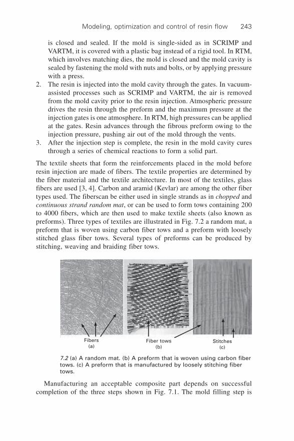
Modeling, optimization and control of resin flow 243
is closed and sealed. If the mold is single-sided as in SCRIMP andVARTM, it is covered with a plastic bag instead of a rigid tool. In RTM,which involves matching dies, the mold is closed and the mold cavity issealed by fastening the mold with nuts and bolts, or by applying pressurewith a press.
2. The resin is injected into the mold cavity through the gates. In vacuum-assisted processes such as SCRIMP and VARTM, the air is removedfrom the mold cavity prior to the resin injection. Atmospheric pressuredrives the resin through the preform and the maximum pressure at theinjection gates is one atmosphere. In RTM, high pressures can be appliedat the gates. Resin advances through the fibrous preform owing to theinjection pressure, pushing air out of the mold through the vents.
3. After the injection step is complete, the resin in the mold cavity curesthrough a series of chemical reactions to form a solid part.
The textile sheets that form the reinforcements placed in the mold beforeresin injection are made of fibers. The textile properties are determined bythe fiber material and the textile architecture. In most of the textiles, glassfibers are used [3, 4]. Carbon and aramid (Kevlar) are among the other fibertypes used. The fiberscan be either used in single strands as in chopped andcontinuous strand random mat, or can be used to form tows containing 200to 4000 fibers, which are then used to make textile sheets (also known aspreforms). Three types of textiles are illustrated in Fig. 7.2 a random mat, apreform that is woven using carbon fiber tows and a preform with looselystitched glass fiber tows. Several types of preforms can be produced bystitching, weaving and braiding fiber tows.
7.2 (a) A random mat. (b) A preform that is woven using carbon fibertows. (c) A preform that is manufactured by loosely stitching fibertows.
Manufacturing an acceptable composite part depends on successfulcompletion of the three steps shown in Fig. 7.1. The mold filling step is
Fibers(a)
Fiber tows(b)
Stitches(c)

Design and manufacture of textile composites244
studied exclusively in this chapter [5–8]. Flow through porous media ismodeled in the following section. In section 7.3, liquid injection moldingsimulation (LIMS), software that is used to simulate resin flow in the moldcavity, is introduced and its utilization in design, optimization and controlstudies is summarized. A method to optimize injection gate location is presentedin section 7.4. Section 7.5 introduces the disturbances associated with themold filling process and explains the major disturbance, racetracking, indetail. Section 7.6 explains the use of feedback control to offset the adverseeffects of racetracking on the mold filling process. In Section 7.7, a passivecontrol method to minimize the defect content in the composite parts ispresented. The chapter is summarized and potential future research directionsare discussed in section 7.8.
7.2 Flow through porous media
In LCM processes, the resin flows through a complex network of channelsand paths that are formed by the architecture of the textile sheets in the moldcavity. The diameters of these channels are several orders of magnitudesmaller than the gap-width of the mold. Thus, in addition to the stresses dueto the presence of textile fibers, the capillary and surface tension effects maybecome significant. The resin flow through the fiber textiles can be characterizedas a complex, dual-scale flow as illustrated in Fig. 7.3. The advance of resinthrough the air channels between tows is a macro-scale flow. The penetrationof resin through the fibers in the tows is a micro-scale flow.
A
B–B Cross-section A–A Cross-section
B
BA Macroscopic flowMicroscopic flow
7.3 Dual-scale flow through the porous medium.
While it is theoretically possible to analyze this complex process in detail,the magnitude of immense computational power required to solve the problemforbids any attempt. Moreover, such a detailed study is not necessary as oneis only interested in the macroscopic flow rate–pressure relationship during

Modeling, optimization and control of resin flow 245
the impregnation of resin. Thus, one would have to average the microscopicstresses to find the macroscopic relationship. The textile preforms are madeup of repeated patterns. Instead of analyzing the entire mold geometry, therepetitive pattern can be identified as a unit cell and the flow can be studiedin detail. The results of this microscopic study can be used determine theresistance to flow through the unit cell in an average sense. Permeability ofa textile preform is defined as the ease of resin flow through the preform.Note that the permeability is an inverse measure of the flow resistance.Extensive research has been conducted to predict and measure the permeabilityof textiles with various architecture. These studies can be grouped in threemajor categories as analytical [9–15], numerical [16–22] and experimental[22–28].
The permeability is used along with Darcy’s law to model the complicatedflow through the porous media in an average sense:
· Ò ◊ — · Òu K = – fh P 7.1
where ·uÒ is the resin velocity vector averaged over the volume, K is thepositive definite permeability tensor of the textile preform, h is the viscosityand —·PÒf is the pressure gradient averaged over the fluid volume. In eqn 7.1,resin is modeled with h and the preform is modeled with K. Note that resinflow through the porous medium is assumed be an isothermal, Newtonianflow, thus resin viscosity is taken to be constant. The resin is assumed to beincompressible, hence the continuity equation can be written as
— · ·uÒ = 0 7.2
Inserting eqn 7.1 into eqn 7.2, the mold-filling process can be written asan elliptic partial differential equation as:
— · (K · —·PÒf) = —K · —·PÒf + K: — (—·PÒf) = 0 7.3
which governs the pressure field in the mold region that is covered withresin. Equation 7.3 is subject to the following boundary conditions (BC):
Neumann BC at the mold walls: n · (k · —f) = 0 7.4
Dirichlet BC at the flow front: P = 0
and at the injection gates: P = Pi,
or: Q = Qi,
where n is the normal to the mold wall and Q is the flow rate. The flow rateboundary condition at a gate can be converted to pressure boundary conditionthrough Darcy’s law. Note that the boundary condition at a gate is appliedalong the boundary of a hypothetical area around the gate in two-dimensional(2D) flow, and over the surface of a hypothetical volume around the gate inthree-dimensional (3D) flow.

Design and manufacture of textile composites246
Figure 7.4 shows domains and boundaries of interest in the mold-fillingprocess. The entire mold cavity forms the mold domain. The region filledwith the resin is the resin domain and eqn 7.3 applies in this domain only. Asthe resin is injected into the mold domain from the gates, the resin domaingrows. Since the resin domain changes with time, the pressure distribution inthe domain changes as well. Also, varying the boundary conditions at theinjection gates modifies the pressure distribution in the resin domain. Therefore,although not explicit in eqn 7.3, the pressure field in the resin domain is afunction of time. The resin flow through the porous medium is low Reynoldsnumber flow, which explains the non-existence of inertia terms in eqn 7.3.Moreover, the flow can be considered to be in quasi-steady state at any giventime step. Dirichlet boundary conditions apply at the free (moving) sectionof the outer boundary of the resin domain, which is called the flow front.Neumann boundary conditions apply at the common boundary of the molddomain and the resin domain.
Free (moving) resin boundary; flow front(Dirichlet boundary condition)
GateVent
Molddomain
Mold boundaryResin domain
Resin-wall boundary (Neumannboundary condition)
7.4 Resin and mold domains and boundaries.
The pressure gradient in eqn 7.1 is created by the pressure applied at thegates, Pi. The injection rate Qi determines the wetted region expansion rate.The relationship between Pi and Qi is a function of the permeability (orresistance) field in the wetted region. One either specifies the pressure Pi orthe flow rate Qi at a gate. As the problem is quasi-steady state, these valuesmay change from one time step to the next time step.
The main function of a vent is to provide an escape passage to the air inthe mold cavity. Mathematically, it enforces the Dirichlet boundary conditionat the flow front. If a contiguous dry region in the mold cavity lacks a vent,the Dirichlet boundary condition in eqn 7.4 does not apply anymore alongthe boundary between the dry region and the resin-covered region. The pressurein the dry region increases owing to compression of air and prevents the

Modeling, optimization and control of resin flow 247
resin from saturating the dry region. It is highly likely that air in such aregion will not be able to escape the mold cavity and will cause a dry spot inthe final composite product, which has to be rejected.
The process modeled by eqns 7.3 and 7.4 is a distributed parameter system,whose solution depends on the mold geometry, permeability field in themold cavity and injection locations and conditions. Since analytical solutionis difficult for 2D and 3D flows, researchers employed numerical methods tosolve it. Various numerical methods have been employed to simulate themold filling step [29–35]. LIMS [36], software developed at the Universityof Delaware to simulate resin impregnation through the porous media, isintroduced in the following section. Note that LIMS can also simulate resincuring during the filling phase, which is not discussed here.
7.3 Liquid injection molding simulation
LIMS uses a finite element/control volume approach to simulate the resinflow in the mold cavity. The finite element mesh of the mold geometry, theresin and textile preform properties (h and K values), gate locations andinjection conditions are input to LIMS as shown in Fig. 7.5. The area arounda node is assigned to the node as its control volume. In Fig. 7.6(a), the nodesat the flow front are marked with solid circles and the control volumes
K h
Material data GeometryGate and ventconfiguration
Command-lineprogramming
Flow fronts Pressure field
7.5 Inputs and outputs of LIMS.

Design and manufacture of textile composites248
around the nodes are circumscribed with dashed squares. The mold filling issimulated recursively as follows:
∑ Step I. t = tnew. LIMS solves eqns 7.3 and 7.4 using finite element methodsto obtain pressure distribution P(x) in the mold at t = tnew.
∑ Step II. The velocity field at the flow front u is determined using eqn 7.1.∑ Step III. Under the current velocity field, the shortest time to fill a new
control volume, Dtmin is found. In Fig. 7.6(b), the mesh is removed tofacilitate visualization and clearly show the smallest area that needs to befilled to saturate the next control volume. Assuming a homogeneouspermeability field, it is clear that the control volume on the top-left willtake shortest time to fill. Thus, Dt is taken such that this control volume isfilled at the next time step.
∑ Step IV. The current velocity field u is applied on the resin flow for Dtmin,the new fill state is estimated and the time is adjusted tnew = tnew + Dtmin.Figure 7.6(c) shows the flow front at the next time step. The discrepancybetween the previous and current flow front locations is highlighted witha different shade in the figure. Note that the top-left control volume iscompletely filled. Also, three new nodes become part of the resin domainat this time step.
∑ Step V. Stop if all control volumes are saturated, otherwise go to step I.
7.3.1 Features of LIMS
Interaction with LIMS
The numerical solver in LIMS is coupled with a scripting language LBASIC.The communication between the user and the solver is provided via a console
t = t1(a)
No mesh(b)
Smallest area to fill in a control volume
Dt : minimum timeto fill the nextcontrol volume
t = t1 + Dt(c)
7.6 (a) Flow front location at t = t1. Flow front nodes are marked withcircles and the associated control volumes are circumscribed withdashed squares. (b) Mesh is removed to facilitate visualization. (c)Flow front location at t = t1 + Dt. Note that the top left node becamepart of the resin domain.

Modeling, optimization and control of resin flow 249
using LBASIC. The process parameters and commands to the numericalsolver are entered from the console. Selected simulation output can be displayedon the console if desired. Also a graphical user interface (GUI) module isavailable to interact with LIMS, which provides point-and-click capabilityfor most common steps. Using LIMS through the GUI module is easier,while the console and LBASIC provide the widest capabilities.
Interrogation of simulation at each time step
In LIMS, each Solve command executes a single loop of the five stepspresented above. Therefore, one can intervene in the simulation at any timestep and modify process and material parameters such as the preform properties,injection location and conditions, or vent locations. Moreover, one can retrievedata from the simulation at any time step. During the actual operation, theoperator can intervene in the process and obtain necessary data.
Procedures
Procedures – batches of LBASIC commands – further facilitate the use ofLIMS. One can create complex algorithms in LBASIC to try various fillingscenarios, retrieve specific data and undertake control actions during moldfilling, as illustrated below.
In Fig. 7.7, a step mold is partially filled and the injection has to beswitched to a secondary gate. Three nodes, Gate A, Gate B and Gate C in the
Gate A Gate A
Potentialsecondary
gatesGate B
Gate C
Firs
t g
ate
Gate C
7.7 Filling contours at progressive times to demonstrate changes infilling patterns when injection gate is switched to secondary Gates A,B or C using the scripting procedures listed in Fig. 7.8.

Design and manufacture of textile composites250
figure, are chosen as the possible locations for the second injection location.Two procedures, TestGates and SwitchGate, are written to try each of theselocations automatically. Initially, the first procedure fills the mold until resinarrives at Gate A and saves the mold filling state in the file State.dmp. Notethat the resin arrives at Gates A, B and C simultaneously. Next, procedureTestGates calls the second procedure three times to try each of Gates A, Band C. Procedure SwitchGate loads the mold filling state from State.dmp,sets the second injection location and completes the mold filling simulation.The procedures are listed in Fig. 7.8 and the flow patterns at various timesteps are illustrated in Fig. 7.7.
Tracers
A tracer simulates a sensor in the mold cavity. It follows the state of a givennode and records the information either to a window on the screen or to atab-limited ASCII file where each line contains the time and traced value.The tracers are valuable tools when one wants to use sensors in resin flowfeedback control studies.
Virtual experimentation environment
LIMS can be called from other programs such as LabView and MATLAB®
through dynamic linking, which provides seamless integration between thetwo environments and computational efficiency. There are two modes ofdata exchange between the LIMS subroutine and the master program:
1. The text (command) data exchange: in this mode, the master programbehaves like a user sitting at the console, sending lines of commands tothe LIMS subroutine and receiving lines of LIMS output. Buffers areused to store information during data exchange between the master programand the LIMS subroutine. Figure 7.9 illustrates schematically an instanceof message traffic between MATLAB and LIMS. In the figure, the lastcommand MATLAB put into the buffer is print socurrenttime(), whichrequests LIMS to print the current simulation time, and the last outputLIMS put into the buffer in response to an earlier request is 342 345.23110000, which can be explained as <node number>, <current simulationtime, i.e. the duration before resin arrives at Node 342>, <pressure atNode 342>. The computational overhead that comes with the messagetraffic limits the amount of data that can be exchanged between theLIMS subroutine and the master program.
2. The binary data exchange: in binary mode, shared memory blocks(memory-mapped file) are used to exchange data between the LIMSsubroutine and the master program (Fig. 7.10). A shared memory block

Modeling, optimization and control of resin flow 251
REM Syntax: TestGates FirstGate, GateA, GateB, GateC, GateType, GateStrengthproc TestGates
defint i, j, FirstGate, GateA, GateB, GateC, GateType, Flag1,defdbl Time, GateStrengthlet FirstGate=argument(1)let GateA=argument(2)let GateB=argument(3)let GateC=argument(4)let GateType=argument(5)let GateStrength=argument(6)let Flag1=1setintype “in”read “onrsmall.in”setgate FirstGate, GateType, GateStrength
REM Fill until the specified limitdo while (Flag1)
solvefor i=1 to sonumberfilled()
let j=sonextfilled()if (j=GateA) then
let Flag1=0setgate FirstGate, 0, 0setouttype “dump”write “State”let Time=socurrenttime()
endifnext i
loopREM Switch injection from the first gate to gates A, B and CSwitchGate GateA, GateType, GateStrength, Time, “State_GateA”SwitchGate GateB, GateType, GateStrength, Time, “State_GateB”SwitchGate GateC, GateType, GateStrength, Time, “State_GateC”
endproc——————REM Syntax: SwitchGate SecondGate, GateType, GateStrength, Time, OutFileproc SwitchGate
defint SecondGate, GateType, GateStrengthdefdbl Timedefstring OutFilelet SecondGate=argument(1)let GateType=argument(2)let GateStrength=argument(3)let Time=argument(4)let OutFile=argument(5)setintype “dump”read “State.dmp”settime Timesetgate SecondGate, GateType, GateStrengthdo while (sonumberempty()>0)
solveloopsetouttype “tplt”write OutFile
endproc
7.8 Two procedures created to try three different filling scenarios.

Design and manufacture of textile composites252
is essentially a data structure that contains all process information. Eachshared block has a name and a certain organization, which allows theLIMS subroutine or the master program to access any specific data fromthe block: the fill factor of a certain node, for example. At any giventime, either the master program or the LIMS subroutine can access thedata block. Note that this exchange mode is binary and does not involveany actual data transfer between the master program and the LIMS
##> print socurrenttime ()
Buffer I
342 345.231 10000
Buffer II
7.9 Text mode data exchange between MATLAB® and LIMS.
Data
Accesscontrol
Node data
Element data
1 byte
Shared memory block
Pro
cess
par
amet
ers
7.10 Binary mode data exchange between MATLAB ® and LIMS.

Modeling, optimization and control of resin flow 253
subroutine; in essence, two software programs share a certain portion ofthe RAM memory. Hence, it is very fast compared with text mode andis suitable for large volume data exchange such as providing data for acontour plot visualization.
The text mode is suitable for small amounts of data exchange and the binarymode is advantageous for large volumes of data exchange. If the same dataare to be accessed repeatedly for a period of time, permanent memory can beused for data exchange. The majority of the study presented in this chapterwas conducted in a virtual optimization and control environment created bythe integration of LIMS and MATLAB® [37], a high-level programminglanguage and an integrated technical computing environment that combinesnumerical computation, advanced graphics and visualization.
7.3.2 Process model in design, optimization and control
Several engineering practices, such as design, optimization and control, requirea mathematical model of the physical system under study. A mathematicalmodel imitates the process physics, and for a given set of process inputs, themodel is expected to reproduce the same results as the actual system. Forexample, in the mold filling process, the inputs are the mold geometry, thegate locations, the injection conditions, the vent locations and the preformand resin properties, and the important outputs are the flow pattern, the filltime, dry spot formations and the pressure requirements.
In some cases an analytical mathematical model is available for the physicalsystem under study:
F = f (x) 7.5
where x represents the process parameters and, f is an explicit function of xthat maps process inputs x to the process output(s) F (Œ R). Several design,optimization and control tools exist to address these types of situations. Inother cases such as the mold filling process, an explicit function that relatesthe process inputs to the process outputs does not exist. Instead, LIMS isused as the mathematical model (also called the process model) of the moldfilling process, which maps the process inputs to the process outputs. Itprovides a virtual testing environment, where one can try different designs,investigate different ideas and concepts, study input–output relations, etc.Common analytical tools in design, optimization and control fields do notapply in these cases, since an explicit form of f is not available. In thefollowing two sections, the utilization of LIMS in the optimization and controlstudies is summarized.

Design and manufacture of textile composites254
Optimization studies
Several design choices exist for the mold in LCM processes. The optimizationalgorithms can help designers achieve the design that fits the performancecriteria best. These algorithms require the mathematical model of the physicalsystem to be optimized. When the mathematical model f is explicitly available,the optimal values of the process parameters x can be estimated using thestandard procedures.
In the mold filling process, LIMS provides the input–output relationship.The cost functions are defined in terms of LIMS output. Several optimizationalgorithms that do not require an analytical process model are available foruse with LIMS [38, 39]. These algorithms are usually iterative. At eachiteration, the process is simulated with the design parameter values from theprevious iteration. The cost function is evaluated using LIMS outputs. Next,the optimization algorithm calculates the new design parameter values, suchas gate locations, for the next iteration. The purpose of all optimizationalgorithms is to converge towards the optimal solution by each iteration [40,41].
Feedback control
During the manufacturing stage, feedback control may be necessary to offsetthe adverse effects of the disturbances and fill the mold successfully. It isstraightforward to simulate the control hardware. Ability to interrogate thesimulation at each time step allows one to simulate actuator actions such asopening/closing a gate and modifying the injection conditions. Sensors aresimulated by using the LIMS output and the tracer data at each time step.The LBASIC procedures are extremely helpful for these purposes.
In the feedback control, once the sensor data have been retrieved from theLCM mold and processed, the optimal control action must be generated bythe controller and sent to the actuators (the gates) to drive the resin flow inthe desired direction. The controller usually will employ a process model topredict the responses to various actuator actions. For such methodology,LIMS can serve as the mold filling process model.
7.4 Gate location optimization
7.4.1 Problem statement
In this section, a gate location optimization problem is stated [39]. The costfunction (also called the performance index) is expressed in terms of LIMSoutput. An assumption on the cost function f is verified using LIMS simulations.
The single gate optimization problem in LCM can be stated as follows:

Modeling, optimization and control of resin flow 255
Given a non-empty, closed set D à R = {integer} and acontinuous function f : D Æ R, find at least one point x* Œ Dsatisfying f (x*) £ f (x) for all x Œ D.
In LCM, x correspond to a node in the finite element mesh where a gate canbe placed and set D consists of all possible x values. f is the cost function thatneeds to be minimized. Note that an analytical expression is not available forf. Instead LIMS output is used to estimate f (x) value. Two assumptions aremade about f.
Assumption I: f (x), x ΠD, is continuous.
Since f is not available, it is impossible to apply standard tests to prove thisassumption. Instead, a case study is presented for verification using simulations.
The bottom picture in Fig. 7.11 is a simplified mesh of a bus chassis.There are two high fiber volume fraction regions in the geometry as illustratedin the figure. Flow resistance is much higher in regions with a high fibervolume fraction. It is desired to find the injection location for a single gatethat will fill the mold in minimum time. The injection would be done undera constant pressure boundary condition. In order to achieve this physically,the resin reservoir is pressurized and held under constant pressure until theresin reaches the last vent. All nodes were tried as injection locations (exhaustivesearch) and corresponding fill times are shown with two surface plots in Fig.7.11. In the plots, the z axis shows the fill time. The lower a node is on thez axis, the less time it takes to fill the mold. The middle picture in Fig. 7.11shows the overall exhaustive search results. As expected, the nodes in thehigh-volume fraction regions are not suitable as the gate location: it takesmuch longer to fill the mold if the injection location is in these regions. Notethat in the middle picture, the results of the high-volume fraction regiondominate the plot; therefore the fill time variation in the remaining regioncannot be further discriminated. In the top picture in Fig. 7.11, the results ofthe high-volume fraction region are removed from the plot, making the behaviorof the remaining nodes visible. As expected, the injection locations in themiddle of the geometry will fill the mold in shorter times. Note that plots inboth middle and top pictures are continuous, hence they verify Assumption I.
Assumption II: df/dx is small and of the same order throughoutthe mesh surface, where dx represents spatial differential of nodex in the mesh.
7.4.2 Branch and bound search
The branch and bound search (BBS) is used as the optimization algorithm[42, 43]. BBS converges on the optimal solution by dividing the solution setinto smaller sets and eliminating the sets that are unlikely to include the

Design and manufacture of textile composites256
optimal solution. This process is repeated until it is no longer possible topartition a set or a stop criterion is met. In order to apply BBS to an optimizationproblem, it should satisfy two requirements.
Requirement I: Given a solution set, it should be possible to estimatea lower bound for the function f.
A lower bound for a solution set Si, i = 1, 2 . . . n, denoted as b(Si), satisfiesthe condition f (x) ≥ b(Si), x Œ Si. The only way to find a lower bound for aset in the current case is to use LIMS with each node in the set, which
High-volumefraction regions
7.11 Bottom: simplified mesh of bus chassis with two high-volumefraction areas. Middle: Surface plot of exhaustive search results. Thegate is desired at a location that will minimize fill time. High-volumefraction regions return high fill times and dominate the plot. Top: Theresults of high-volume fraction region are removed from the plot,which clearly shows that the gate should be placed at the center.

Modeling, optimization and control of resin flow 257
amounts to impractical exhaustive search. Hence, in this study, the lowerbound is replaced with a qualitative parameter as follows.
Owing to the physics of the problem, f can take in multiple values andreturn a single value: f = f ([x1, x2 . . . xn]), x ΠD, i.e. multiple gates can beused simultaneously to fill the mold, which will yield a single flow patternthat will return a single f value. Given a set Si, the pseudo-average of f overthe set is defined as fSi = f (Si), i.e. all nodes in the solution set Si aresimultaneously designated as gates and the subsequent value of the costfunction f is assigned to fSi
. A third assumption is derived from AssumptionII as follows:
Assumption III: For the sets at the same partitioning level, thedifferences between the pseudo-average fSi
and the unknownlower bound b(Si) is of the same order: ei ~ avg (ei), where ei =| fSi – b(Si)|.
According to Assumption III, fSi = b(Si) ± ei. Since ei varies slightly for sets
under evaluation, fSi can replace unknown b(Si) for the purpose of rankingthe performances of various solution sets.
Requirement II: There should be a way to partition a givensolution set.
The solution set is partitioned according to geometrical guidelines (Fig.7.12). Although there are standard partitioning methods in BBS, none hasyet been proven to be applicable to the mold filling problem. A rule of thumb
Region 3 Region 6 Region 9
Region5 Region 8Region 2
Region 1 Region 4 Region 7
7.12 Recursive domain reduction in branch and bound search whileconverging on the optimal solutions.

Design and manufacture of textile composites258
is to partition the set in a way to validate Assumption III. A fine partitioningshould be used for sets that include high gradients of f, whereas sets with lowgradients may perform well with a coarse partitioning. A major cause of highgradients is significant variations to the permeability distribution within thearea covered by the set. In this study, homogeneous, equal partitioning isused regardless of the permeability field in the mold.
Procedure
The algorithm of the BBS is explained step by step below. The nodes in theentire mesh are taken as the first solution set.
∑ Step 1: Partition the set(s) into subsets to form a new group of smaller setsfor evaluation.
∑ Step 2: For each set in the group estimate fSi .∑ Step 3: Choose the set with fmin = min ( fSi ). Also choose the sets whose
f values are close to fmin in order to compensate for the imprecisenessin Assumption III.
∑ Step 4: Remove the remaining sets from the search space.∑ Step 5: If the chosen sets include suffcient number of nodes for partitioning,
go to Step 1. Otherwise, simulate mold filling for each node in the chosenset(s), take the best solution and Stop. In this study, partitioning is continueduntil there are four or fewer nodes in a chosen set.
A schematic explanation of the procedure is given in Fig. 7.12: A 3 ¥ 3partitioning scheme is used throughout the solution. In the first iteration, sets2 and 6 give superior performance as compared with other sets and hence,are selected for the next level of subdivision. In order to reach the optimalsolutions, three iterations were suffcient as illustrated in the figure.
In the following section, BBS is used to find the gate location in a boxgeometry that will fill the mold in minimum time.
7.4.3 Case study: minimum fill time
During an injection system design, filling the mold as quickly as possible isan important goal as it will reduce the cycle time and increase the profitabilityof the process. Also for quick-curing resins, it lowers the possibility of resingelling and hardening before the mold is completely filled. The mold ofinterest and its mesh are illustrated in Fig. 7.13(a). It is a two chamber, 65 ¥30 ¥ 25 cm3 hollow box, and the dividing wall has a circular hole in it. Themesh of the mold has 3378 nodes and 3316 elements.
An injection system with a single gate is designed. The resin is injectedthrough the gate under the constant pressure of 0.2 MPa. The resin viscosityis assumed to be 0.1 Pa s. The preform is assumed to be isotropic with a

Modeling, optimization and control of resin flow 259
permeability of 10–6 m2. The gate is desired at a location on the mold geometrythat will minimize the fill time. Hence, the cost function for this problem isas follows:
f = f (x): the fill time 7.6
where x is the location of the single gate. The vents are placed in the lastregions to fill or the mold can be assumed to be under perfect vacuum, so thepossibility of having dry spots is non-existent. For a given set Si, pseudo-average fSi = f (Si) is estimated by equating the injection pressures of eachnode in the set to the preselected constant pressure value, �x Œ Si, P(x) =Pinjection and then simulating mold filling using LIMS.
Initially, the problem is solved using the exhaustive search (ES). After3378 simulations, ES showed that the optimal gate location is at Node 1756(x = 30 cm, y = 16.5 cm, z = 0 cm) with a fill time of 1000 seconds. Node1756, which is located on a hidden line, is marked with an ellipse in the left-hand figure in Fig. 7.13. During BBS, a 3 ¥ 3 ¥ 3 partitioning is appliedthroughout the optimization procedure. After a total of 3 iterations and 57simulations, BBS arrived at the same result. Overall, BBS was 98% moreefficient computationally than ES, which illustrates the advantages ofoptimization algorithms. More details and examples can be found in Gokce[5] and Gokce and Advani [44].
7.5 Disturbances in the mold filling process
During the mold filling stage of LCM processes, the textile sheets must becompletely saturated with resin. The gates and the vents must be placedappropriately to ensure complete saturation. Usually, the gate locations arechosen first to achieve certain objectives such as minimum fill time, andminimum pressure requirements. Next, the vents are placed at locations
7.13 Left: box mold. Right: the mesh of the box mold andpartitioning scheme.
Z
YX
20
10
00
60
40
20
01756

Design and manufacture of textile composites260
where resin arrives last.1 Such design decisions are made based on the processmodel and subsequent simulations. If the actual values of the process parametersare significantly different from the predicted values, then the subsequentdesigns may fail to satisfy the intended objectives.
The constitutive relationship between the resin velocity field and the pressurefield in the mold cavity is a function of the resin viscosity and the permeabilityfield as stated by eqn 7.1. Variations in these two parameters may cause themold filling stage to go astray, resulting in a defective part. In the moldfilling process, the fill time and the flow pattern are important output variables.The fill time is the total duration of the mold filling process and is a functionof several parameters such the resin viscosity, permeability field and theinjection conditions. The flow pattern can be defined as the filling sequenceof the mold cavity by the resin. The flow pattern is a function of the normalizedform of the permeability field in the mold cavity. The fill time and the flowpattern are independent of each other.
The variations in the resin viscosity and the permeability field cause thefill time and the flow pattern to vary. Variations in the fill time are tolerable.A very small fill time implies fast filling of the mold, which may causemicro-bubbles in the fiber tows, an issue not addressed here. If the moldfilling stage takes too much time, resin may start gelling, which will complicateand possibly fail the mold filling operation. On the other hand, variations inthe flow pattern may cause significant defects in the composite part. Sincegates and vents are placed into the mold based on a predicted flow pattern,a moderate alteration in the flow pattern due to disturbances may cause thegate and vent design to fail. Hence, variations in the flow pattern are morecritical than the variations in the fill time. Some disturbances that may influencethese two outputs are summarized below.
∑ Resin viscosity: Variations in the resin viscosity h, may cause the resin toflow slower or faster and affect the fill time. Under certain conditions, theisothermal-Newtonian flow assumption may fail. If the resin begins to gelbefore the entire mold is filled owing to faulty chemical composition,its viscosity will increase by several orders. Consequently, the resin flowwill slow down in certain parts of the mold cavity and alter the flowpattern.
∑ Defects in the preform: Manufacturing defects or impurities in the textilepreform may cause local variations in the permeability field. As a result,resin may flow faster or slower at certain parts of the mold, changing theflow pattern. Note that major preform defects can be detected easily before
1Note that the term last is not used in the chronological sense. It means the last region tofill in a contiguous dry area, after which the dry area disappears, regardless of the timescale.

Modeling, optimization and control of resin flow 261
the preforms are placed into the mold and minor defects do not causesignificant disturbances. Hence, this is a minor issue.
∑ Textile preform compaction during mold closing: In LCM processes, thetextile sheets in the mold cavity are under pressure. (This pressure is notrelated to the injection pressure applied at the gates.) In vacuum-assistedprocesses with single-sided molds, atmospheric pressure is applied on thetextile sheets through the plastic covering. In matched die molds, thepressure on the preform can be much higher, depending on the number ofpreform layers and the preform architecture. Depending on the pressurelevel, the fiber architecture may change in various ways, affecting theshape of the flow channels, which determine the permeability of the porousmedium, as illustrated in Fig. 7.14(a). In general, compaction affects thepreform permeability globally, hence it may affect the fill time but not theflow pattern.
∑ Interaction of textile layers during mold closing: Since architecture ofmost textile preforms consists of repeated patterns, there are regions with
7.14 Interaction of preform layers in a closed mold: (a) compaction:the preform layers become thinner under pressure; (b) nesting:preform layers mesh with each other under pressure. There is nonesting on the left figure, whereas there is a significant level ofnesting on the right figure.
Fiber tows
h
h
(a)
P
Mold wall
H(< 2h)
Mold wall
P
PPMold wall
Mold wall
Mold wallMold wall
P
Singlepreform
layer
(b)
P

Design and manufacture of textile composites262
high and low fiber fractions. Under pressure, the textile preform layersprotrude into each other as illustrated in Fig. 7.14(b), a phenomenoncalled the nesting effect. The level of nesting effect is a function of therelative position of textile sheets with respect to each other and the appliedpressure on the textile preform. The nesting effect influences the structureof flow channels in the mold cavity, hence the permeability field of theporous medium. Its effect on the permeability field is global, hence it doesnot affect the flow pattern. In this case the nesting effect is related to thecompaction of textile sheets.
∑ Accidental flow paths in the mold cavity: Especially in matched die molds,the mold cavity is rigid. Achieving an exact fit between the textile preformand the mold cavity is a difficult challenge. When there are gaps betweenthe inner mold surface and the textile preforms, channels that offer lowresistance to resin flow may be created unintentionally in the mold cavity.Resin flows faster in these channels, altering the flow pattern significantly,a phenomenon known as racetracking. Figure 7.15 shows an example ofaltered flow front due to a gap along an edge. These channels, calledracetracking channels, are more likely to form at certain locations in themold as shown in Fig. 7.16. Several researchers have attempted to modelthese channels and their effects on the flow pattern [47–53]. Traditionally,the textile preform is assumed to fit the mold cavity exactly. However,because of process variations during preform cutting/placement and preformcompaction mechanisms during mold closing, it is diffcult to achieve aperfect contact between the bulk preform and the inner mold surface.Consequently, racetracking emerges as the most common disturbance inthe mold filling stage of the certain LCM processes.
7.15 Experimental snapshots of racetracking along the left edge of arectangular mold cavity [45, 46]. The resin enters the mold cavityfrom a line injection gate along the upper edge. Horizontal flowfronts would be developed if there was no racetracking.
The flow pattern, the key measure of successful mold filling, is a functionof the racetracking conditions, which depend on the state of the contactbetween the textile preform and the inner mold surface. Since the contact

Modeling, optimization and control of resin flow 263
state is unrepeatable from one experiment to the other, racetracking is amajor cause of process unrepeatability in the mold filling process. Becauseof its frequent occurrence and significant adverse effects, racetracking is theonly disturbance studied in this chapter. However, the tools and methodologiesdeveloped for racetracking can be applied to other disturbances.
7.5.1 Modeling a racetracking channel
A racetracking channel is created because the resistance to flow along acertain path is affected by the type of fiber architecture, precision of a cutand placement of the textile preform. Resin flow through a racetrackingchannel usually meets a lower resistance than the textile preform, hencepermeability along a racetracking channel is higher. The resin flow in thechannel can be modeled as slow, fully developed, steady-state viscous ductflow and one can develop an equivalent permeability expression for it interms of channel dimensions as [49, 52, 54]:
K a ab
i b aiirt
2
5 =1,3,5.. 5 = 12
1 – 192 tanh ( /2 )
ppS
•ÈÎÍ
˘˚
7.7
where Krt is the equivalent permeability of the racetracking channel, b is thedistance between the preform and the mold wall and a is the height of themold cavity (Fig. 7.17). Note that the wider the gap between the preform andthe mold wall, the stronger will be the racetracking.
The equivalent permeability of the racetracking channel in eqn 7.7 is not
Mold wall
Sidewall
(a) (b)
(c) (d)
Side view
Mo
ld w
all
Missing tow
Top view
7.16 Various situations that cause racetracking: (a) poor dimensionalcontrol during perform cutting; (b) low volume fraction at the edges,possibly due to missing fiber tows; (c) insufficient mold closing; (d)poor mold design.

Design and manufacture of textile composites264
suffcient to quantify racetracking alone. The ratio of the equivalent permeabilityKrt to the textile preform permeability Kpreform is chosen as a measure of theracetracking strength;
r = rt
preform
KK
7.8
where r is the racetracking strength. Note that Kpreform can vary by severalorders of magnitude for various preforms. Table 7.1 shows racetrackingstrength for five different preforms with an identical racetracking channel of0.5 mm wide and 6.35 mm high. In the simulation environment, these fivepreforms are placed in a rectangular mold successively such that a 0.5 ¥ 6.35mm2 racetracking channel is along the top edge. The injection gate is placedon the left edge and mold filling is simulated under constant flow rate injectionfor all five cases: r = {1, 4.1, 52.5, 124.5, 562.5}. Note that r = 1 meansthere is no racetracking in the mold. The flow front positions at the sametime step for all five cases are superimposed in Fig. 7.18. The higher theracetracking strength r, the more resin flow deviates from the nominal case(r = 1). Figure 7.18 shows that even if the racetracking dimensions areidentical in all the cases, racetracking takes place at varying levels as it is afunction of the permeability of the textile preform as well.
A racetracking channel is not likely to have a perfect duct shape as in Fig.7.17. The dimensions of the channel, a and b, in eqn 7.7 may vary along thechannel; a = a(s) and b = b(s), where s is the coordinate along the length of
Racetrackingchannel
Mold wall
Bulkpreform
Cross-section b
a
Racetrackingchannelmodel
7.17 Modeling of resin flow in the racetracking channel as duct flow.
Table 7.1 Racetacking strengths for various performas with identical racetrackingchannels
Type of preform [55] Preform Racetrackingpermeability (m2) strength, r
Random glass fiber 4.88 ¥ 10–9 4.13D woven glass fibers 3.77 ¥ 10–10 52.5Unidirectional (warp) 1.59 ¥ 10–10 124.5woven glass fibersNon-woven stitched glass fiber 3.53 ¥ 10–11 562.5
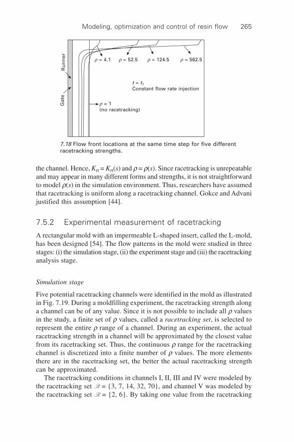
Modeling, optimization and control of resin flow 265
the channel. Hence, Krt = Krt(s) and r = r(s). Since racetracking is unrepeatableand may appear in many different forms and strengths, it is not straightforwardto model r(s) in the simulation environment. Thus, researchers have assumedthat racetracking is uniform along a racetracking channel. Gokce and Advanijustified this assumption [44].
7.5.2 Experimental measurement of racetracking
A rectangular mold with an impermeable L-shaped insert, called the L-mold,has been designed [54]. The flow patterns in the mold were studied in threestages: (i) the simulation stage, (ii) the experiment stage and (iii) the racetrackinganalysis stage.
Simulation stage
Five potential racetracking channels were identified in the mold as illustratedin Fig. 7.19. During a moldfilling experiment, the racetracking strength alonga channel can be of any value. Since it is not possible to include all r valuesin the study, a finite set of r values, called a racetracking set, is selected torepresent the entire r range of a channel. During an experiment, the actualracetracking strength in a channel will be approximated by the closest valuefrom its racetracking set. Thus, the continuous r range for the racetrackingchannel is discretized into a finite number of r values. The more elementsthere are in the racetracking set, the better the actual racetracking strengthcan be approximated.
The racetracking conditions in channels I, II, III and IV were modeled bythe racetracking set R = {3, 7, 14, 32, 70}, and channel V was modeled bythe racetracking set R = {2, 6}. By taking one value from the racetracking
Gat
eR
un
ner
r = 1(no racetracking)
t = t1Constant flow rate injection
r = 4.1 r = 52.5 r = 124.5 r = 562.5
7.18 Flow front locations at the same time step for five differentracetracking strengths.

Design and manufacture of textile composites266
set of each channel, 1250 (5 ¥ 5 ¥ 5 ¥ 5 ¥ 2) racetracking scenarios werecreated. The collection of all scenarios is called a scenario space S.
The mold filling was simulated for all 1250 racetracking scenarios.2 Sevenpoint sensor locations were identified in the mold for racetracking measurements(Fig. 7.19). A table that includes resin arrival times at the sensors for allscenarios was created from the simulation results. The table, called the detectiontable, would be used to compare simulation results with the experimentalarrival times to identify the racetracking scenario that is closest to the moldfilling state in the mold.
Experiment stage
A rectangular mold and an L-shaped insert were manufactured and assembledto create an L-mold. Point sensors and a CCD camera were used as thesensors (Fig. 7.20). Fifty mold filling experiments were conducted using thesame mold and materials under the same processing conditions. During eachexperiment, resin arrival times at the point sensors were recorded to identifythe closest scenario from the scenario space S. Note that actual racetrackingstrength in a racetracking channel will probably not be equal to any of thevalues in the racetracking set associated with the channel. Consequently, anactual flow pattern will not exactly match any of the 1250 racetrackingscenarios. However, this is a source of error common to all discretizationoperations. If the discrete case is suffciently close to the actual case, then theresults returned by the discrete case will be within the range.
Rac
etra
ckin
gch
ann
el V
Racetracking channel II
Racetracking channel IV
Racetracking channel III
Point sensors
Line so
urce
Racetracking channel I
7.19 Potential racetracking channels and sensor locations in the L-mold.
2To make the text more readable, the term scenario will be used to represent a mold(filling operation) with specific racetracking conditions. Therefore, the phrases a scenariois filled/drained/saved must be understood accordingly.

Modeling, optimization and control of resin flow 267
Racetracking analysis
The flow pattern of each experiment was approximated by a racetrackingscenario using the detection table. Thus, 50 r measurements were obtainedfor each of the five racetracking channels in the mold. The frequency of theelements in set Ri of racetracking channel i is displayed and plotted in Fig.7.21. The data show that racetracking occurred frequently at varying levelsin all channels, which illustrates the significance of racetracking.
7.5.3 Successful mold filling despite racetracking
Traditionally, in RTM processes the gate locations are selected first and thenvents are placed at the last-filled regions. The case without any disturbancesis called the nominal case and the corresponding vent configuration is calledthe nominal vent configuration. Racetracking even at moderate levels canalter the flow pattern significantly and cause the resin to arrive at the ventsearlier, blocking the air drainage. The nominal vent configuration, which wasdesigned for the nominal flow pattern, cannot drain the air successfully foran altered flow pattern. There are two approaches to address the disagreementbetween the altered flow pattern and the nominal vent configuration:
1. Active control: One way is to counteract the influence of racetracking onthe flow pattern using feedback control. The resin flow is steered bymodifying the injection conditions at the gates towards the existing(nominal) vent configuration so that all air is drained from the moldcavity.
Inner moldsurface
Wires
Videocamera
Lineinjection
Pressurepot
L-mold
7.20 (a) A point sensor; (b) Experimental set-up [56].

Design and manufacture of textile composites268
2. Passive control: The vents act as constraints on the mold filling processby dictating the last points resin must arrive for a successful mold filling.Instead of driving the resin towards a nominal vent configuration as infeedback control, one might take the inverse approach and augment thenominal vent configuration by adding more vents, hence relaxing theconstraint on the mold filling process. A suffcient number of vents canbe placed optimally in the mold such that there will always be a vent inthe vicinity of a region where resin arrives last.
7.6 Active control
The central idea in feedback control is to manipulate the resin flow in themold cavity by modifying the injection conditions at the gates. A feedbackcontrol system has three major components:
1. Data acquisition hardware: This includes the sensory system and signalprocessing circuitry. The sensory system provides data from the closedmold, which enables one to track resin flow in the mold cavity. Thesensors used to monitor mold filling can be direct current (DC), dielectric,optic, ultrasound or microwave-based, and can be classified in variousways depending on the method used, such as point-sensing versus
Frequency of discrete rvalues
r value R I R II R III R IV
3 2 12 4 307 2 14 4 10
14 12 22 17 732 34 0 10 170 0 2 15 2
r value R V
2 386 12
R V
40
35
30
25
20
15
10
5
0
Freq
uen
cy
2 6r
35
30
25
20
15
10
5
0
Freq
uen
cyR IV
R III
3 7 14 32 70r
40
3530252015
10
5
0
Freq
uen
cy
R II
R I
3 7 14 32 70r
7.21 Experimental outcomes for racetracking channels in the L-mold.

Modeling, optimization and control of resin flow 269
continuous-sensing sensors, or intrusive versus non-intrusive sensors.The variables that are measured by the sensors can be conductivity,impedance, electric current and reflection properties of light/laser beams,ultrasound waves or microwaves. Signal processing cards usually comewith the sensory system, otherwise these are available off-the-shelf.
2. Controller: This is a computer program that can evaluate the incomingprocess data and generate input signals for the gates that will manipulatethe resin flow in the desired direction.
3. Actuators: These are the controllable process inputs that drive the physicalsystem. In the mold filling process, the only actuators are the injectiongates in the mold. One can manipulate the resin flow by varying theinjection conditions at the gates.
The control methods that were used for the mold filling process can bedivided into two as set point-based control and scenario-based control. Inset point-based control, the injection system with two or more gates and acertain number of vents is designed at first. A target flow pattern – usuallythe nominal flow pattern – is designated. During the mold filling operation,the control is conducted periodically: during a sampling time Dt, the flowfront position is determined through the sensors and is compared with thetarget flow front position at the current time step. The error is estimated and,based on the traction error, the controller generates the optimal input signalsfor the injection gates to minimize the error between the actual and targetflow front position. Neural networks, adaptive control and model-based controlare some of the set point-based control methods [57–61].
There is an offine stage and an online stage in the scenario-based control.In the offline step, the injection system is designed for the nominal case. Ascenario space that aims to model the disturbances is created. The sensorysystem is designed and detection tables are created to identify scenarios inthe closed mold. Auxiliary injection gates are placed into the mold. Usingvarious algorithms, control actions that fill each scenario successfully aredetermined, concluding the offline stage. The online stage can divided intotwo: the recognition step and the control step. During the recognition step,the sensory system tracks the resin flow and associates it with a scenariofrom the scenario space. Once the closest scenario has been found, theassociated control actions are undertaken in an open-loop manner. Decisiontrees, genetic algorithms (GA) and ES are used for scenario-based control[7, 62, 63].
7.6.1 Simulation-based liquid injection control (SLIC)
A scenario-based learning control system has been developed at the Universityof Delaware [63]. The system, named Intelligent RTM, consists of an offline

Design and manufacture of textile composites270
stage called simulation-based liquid injection control (SLIC) and an onlinestage called AutoRTM, which is a LabView program. Intelligent RTM haseight modules:
∑ Level 0: Given the mesh of the part, nominal material parameters and thedisturbance ranges, a scenario space is created.
∑ Level 1: The injection system for the disturbance-free case is designed.Optimal gate and vent locations are determined simultaneously using GA.
∑ Level 2 (Only for LCM processes that utilize distribution media): Thedistribution media for the part is designed for the disturbance-free case.
∑ Level 3: The locations of the auxiliary gates that will undertake controlactions and the locations of the point sensors that will activate the gatesare determined optimally using GA. The auxiliary system is tested in thescenario space.
∑ Level 4: A sufficient number of vents are placed optimally in the moldusing GA and detection tables are created to choose the scenario from thescenario space that is closest to the actual mold filling state.
∑ Level 5: The data from the offline stage are converted into a form (LabView format) that is usable by the online components of the system. Thisstep completes the offline stage of the control system. The mold fillingoperation can be initiated and controlled using the data from the offlinestage.
∑ Level 6: When a racetracking scenario that does not belong to the scenariospace takes place during mold filling, it is added to the detection table andcontrol actions that will fill the scenario successfully using the existinghardware are sought offline. This learning ability gives flexibility to SLIC.
∑ Level 7 (under development): Performance statistics reports that includethe composite quality, cycle time and cost are prepared automatically.
7.6.2 Case study: rectangular mold with triangular insert
SLIC is demonstrated on a rectangular part with a triangular insert as shownin Fig. 7.22. The top and bottom edges, and three edges of the triangle areidentified as potential racetracking channels. In all channels, the racetrackingstrength is modeled with the racetracking set R = {20, 100}, which yields ascenario space with 25 = 32 scenarios. The resin is injected from two injectionlines on the left and right edges of the geometry. Auxiliary gates are placedoptimally into the mold and the control actions that fill each scenariosuccessfully are determined in level 3. In level 4, the scenario detectionsensors are placed into the mold and a detection table is created. The snapshotsfrom an experiment are illustrated in Fig. 7.23 along with the flow pattern ofthe associated scenario, scenario 29 with r = 100 in channels 1, 2 and 5 andr = 20 in channels 3 and 4. After the detection stage, the control actions
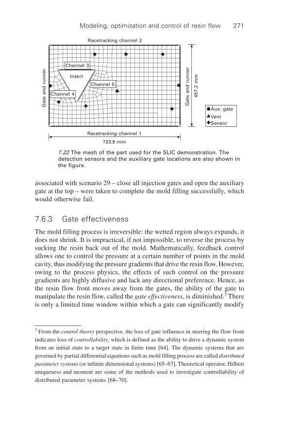
Modeling, optimization and control of resin flow 271
associated with scenario 29 – close all injection gates and open the auxiliarygate at the top – were taken to complete the mold filling successfully, whichwould otherwise fail.
7.6.3 Gate effectiveness
The mold filling process is irreversible: the wetted region always expands, itdoes not shrink. It is impractical, if not impossible, to reverse the process bysucking the resin back out of the mold. Mathematically, feedback controlallows one to control the pressure at a certain number of points in the moldcavity, thus modifying the pressure gradients that drive the resin flow. However,owing to the process physics, the effects of such control on the pressuregradients are highly diffusive and lack any directional preference. Hence, asthe resin flow front moves away from the gates, the ability of the gate tomanipulate the resin flow, called the gate effectiveness, is diminished.3 Thereis only a limited time window within which a gate can significantly modify
Racetracking channel 2
Channel 3
Insert
Channel 5
Channel 4
Gat
e an
d r
un
ner
Racetracking channel 1
723.9 mm
Gat
e an
d r
un
ner
457.
2 m
m
Aux. gate
VentSensor
7.22 The mesh of the part used for the SLIC demonstration. Thedetection sensors and the auxiliary gate locations are also shown inthe figure.
3 From the control theory perspective, the loss of gate influence in steering the flow frontindicates loss of controllability, which is defined as the ability to drive a dynamic systemfrom an initial state to a target state in finite time [64]. The dynamic systems that aregoverned by partial differential equations such as mold filling process are called distributed
parameter systems (or infinite dimensional systems) [65–67]. Theoretical operator, Hilbertuniqueness and moment are some of the methods used to investigate controllability ofdistributed parameter systems [68–70].

Design and manufacture of textile composites272
the resin flow pattern. This phenomenon is illustrated in the simulationenvironment with a case study below.
Mold III, a long rectangular mold with a line resin source on the far leftand an injection gate on the bottom edge, is designed as illustrated in Fig.7.24(a). Resin proceeds in straight lines from left to right. A coordinatesystem is attached to the mold such that its origin coincides with the point
Time 0, both initial injection lines areopened automatically
Detectionstage
Flow reached 3 sensor locationsout of 5 (t1, t2, t3 are known).
Detection phase still under way
Detectiondatabase
Control actiondatabase
Resin arrival timest1, t2, t3, t4, t5 at all
five sensors arecollected
Scenario 29is selected
Correspondingcontrol action
is initiated
Controlstage
Control action 29 is in progress. Gate G1 isopened and initial lines are closed when
resin reaches control action trigger sensorS31 and initial lines are turned off when S27
is reached.
Successful injection
Initial injectionlines
Fixed ventControl gates
Sensors for control actionSensors for identification
7.23 Snapshots from a mold-filling experiment. The flow pattern wasidentified as scenario 29 from the scenario space and the associatedcontrol actions were taken to achieve complete filling.
S27
G1
G2
S31

Modeling, optimization and control of resin flow 273
gate location and its x axis is aligned with the flow direction. Principaldirections of the permeability tensor are aligned with x and y directions andthe preform is isotropic: Kxx = K11 = Kyy = K22. The gate is initially closed.In the first case, the gate is switched on as soon as the flow front arrives there(Fig. 7.24b). In the second case, flow is allowed to proceed until x = 0.3W,where W is the width of the mold (Fig. 7.24c), before the point gate isswitched on. In the final case, the gate is turned on when the flow is at x =0.6W (Fig. 7.24d). In all cases, the line source at the left edge is turned offwhen the gate is turned on. The simulations show that the effect of the gateon the flow front strongly depends on the position of the gate location withrespect to the flow front position.
Since the flow front is continuously steered through a set of injectiongates in set point-based control, the gate effectiveness is more crucial in thiscase. The gate effectiveness has been addressed as a secondary topic in a fewstudies [58, 60]. Gokce and Advani studied gate effectiveness in one-dimensional flow and used the results to derive guidelines for the gateeffectiveness in higher-dimensional flows [71]. They investigated theeffectiveness of the gate in Mold III through a statistical study by varying thevertical location of the gate and the flow front location separately.
x
Gate
Lineinjectionsource W
(a) (b)
0.6 W (d)0.3 W (c)
7.24 (a) Mold III, a rectangular mold with a line injection at the leftand an injection gate at the bottom. (b) The gate at x = 0 is switchedon as soon as the flow reaches it. (c) The gate at x = 0 is switched onafter the flow reaches x = 0.3W, where W is the width of the mold.(d) The gate at x = 0 is switched on after the flow reaches x = 0.6W.In all cases, the flow proceeds from left to right from a constant flowrate line injection source on the left. When the gate is switched on,the line source is switched off.
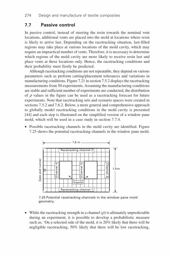
Design and manufacture of textile composites274
7.7 Passive control
In passive control, instead of steering the resin towards the nominal ventlocations, additional vents are placed into the mold at locations where resinis likely to arrive last. Depending on the racetracking situation, last-filledregions may take place at various locations of the mold cavity, which mayrequire an impractical number of vents. Therefore, it is necessary to determinewhich regions of the mold cavity are more likely to receive resin last andplace vents at these locations only. Hence, the racetracking conditions andtheir probability must firstly be predicted.
Although racetracking conditions are not repeatable, they depend on variousparameters such as preform cutting/placement tolerances and variations inmanufacturing conditions. Figure 7.21 in section 7.5.2 displays the racetrackingmeasurements from 50 experiments. Assuming the manufacturing conditionsare stable and sufficient number of experiments are conducted, the distributionof r values in the figure can be used as a racetracking forecast for futureexperiments. Note that racetracking sets and scenario spaces were created insections 7.5.2 and 7.6.2. Below, a more general and comprehensive approachto globally model racetracking conditions in the mold cavity is presented[44] and each step is illustrated on the simplified version of a window panemold, which will be used in a case study in section 7.7.4.
∑ Possible racetracking channels in the mold cavity are identified. Figure7.25 shows the potential racetracking channels in the window pane mold.
1.6 m
Racetracking channel 2
Ch
ann
el 5
Ch
ann
el 4
Ch
ann
el 3
1.0m
Inserts
Racetracking channel 1
Gat
e an
d r
un
ner
7.25 Potential racetracking channels in the window pane moldgeometry.
∑ While the racetracking strength in a channel (r) is ultimately unpredictableduring an experiment, it is possible to develop a probabilistic measuresuch as, ‘On a selected side of the mold, it is 20% likely that there will benegligible racetracking, 50% likely that there will be low racetracking,

Modeling, optimization and control of resin flow 275
20% likely that there will be medium racetracking and 10% likely thatthere will be strong racetracking’. Density functions from the probabilitytheory are utilized as probabilistic measures of the racetracking conditionsin the channels. The probability that the racetracking strength in a channelwill occur within a certain range, r1 ≥ r ≥ r2, can be estimated from adensity function. The density function that characterizes racetrackingbehavior in a racetracking channel is called as the racetracking forecast.The ideal way to obtain the density function is to use process statisticsfrom the manufacturing floor. The tolerances of preform cutting and theequipment used to place the fabrics in the mold, plus the experience of theoperators, will also influence the density function. Density functions canbe derived only under steady manufacturing conditions, and the degree ofagreement between the density function and the actual racetrackingconditions in the mold will influence the efficiency of the optimizedresults on the manufacturing floor. Variations of Weibull density function(Fig. 7.26a) are used to model racetracking conditions in the window panemold.
g( r
)
0.180.160.140.12
0.10.080.060.040.02
20 40 60 80r
(a)
g( r
)
0.180.160.140.12
0.10.080.060.040.02
20 40 60 80r
(b)
7.26 (a) Weibull probability density function. (b) Continuousprobability density function is discretized into a racetracking set withfive racetracking values.
∑ The density functions are usually continuous. Since a continuous functionis not usable in optimization studies, it is discretized into a racetrackingset, Ri = {r1, . . . , rm}, where i is the index of the racetracking channeland m is the number of elements in the racetracking set. Each element inthe racetracking set represents a r interval from the r range. A probabilityvalue is calculated for each element in R from the density function. Thelikelihood that an actual racetracking value will be in a certain r intervalis given by the probability value of the R element which represents thatinterval. The sum of the probability values is equal to 1. All five density

Design and manufacture of textile composites276
functions used for the window pane mold are discretized into four rvalues as shown in Table 7.2 and corresponding probability values areestimated from the Weibull density function (Fig. 7.26b).
Table 7.2 Racetracking sets of the channels in the window pane mold andassociated probability values
Racetracking set Associated probability values
Channel 1 C1 = {1, 10, 30, 100} P1 = {0.44, 0.31, 0.20, 0.05}Channel 2 C2 = {1, 10, 30, 100} P2 = {0.44, 0.31, 0.20, 0.05}Channel 3 C3 = {1, 10, 25, 80} P3 = {0.39, 0.35, 0.19, 0.07}Channel 4 C4 = {1, 10, 25, 80} P4 = {0.39, 0.35, 0.19, 0.07}Channel 5 C5 = {1, 10, 25, 80} P5 = {0.39, 0.35, 0.19, 0.07}
∑ After all channels are modeled with appropriate racetracking sets, a scenariospace S is created by taking all possible racetracking arrangements: C1 ¥C2 ¥ . . . ¥ Cn, where ¥ is the Cartesian product4 operator and n is thenumber of racetracking channels in the mold. Each scenario represents aprocess window that may take place during the actual mold filling processand has a certain probability of occurrence. Assuming the racetrackingforecast of each channel is independent of the other racetracking channels,the probability of each scenario is estimated by multiplying the probabilityvalues of the racetracking set elements that make up the scenario. Theprobability of a scenario determines its weight in the scenario space,which has a total probability of 1. With the addition of the probabilitydimension, the scenario space represents mold filling conditions, includingpreform cutting and placement operations. Practically, it predicts whatmight happen during mold filling on the manufacturing floor. Note thatscenario space is an approximation to the racetracking forecast. As for thewindow pane mold, the scenario space is created by taking the Cartesianproduct of the racetracking sets, C1 ¥ C2 ¥ C3 ¥ C4 ¥ C5, which yields 1024scenarios. The runner location on the left edge was known beforehand,which simplified the racetracking modeling. Otherwise, the scenario spaceis independent of the gate locations and injection conditions.
7.7.1 Optimization problem
The locations of the vents do not have an effect on the mold filling processuntil resin arrival. Assuming they are closed shortly after resin arrivals, vent
4 The Cartesian product in set theory resembles outer multiplication operation in tensor
notation, except that the operands are not actually multiplied in the Cartesian product butare grouped together.

Modeling, optimization and control of resin flow 277
locations act as a constraint on the mold filling process, rather than a processvariable.
Constraint I. At any given time during mold filling t = ti, eachcontiguous air bubble in the mold cavity must have at least onevent within its volume; p(V ) : Di « V π 0, where p is theconstraint, Di is the set of nodes in the contiguous air bubble iand V is the vent configuration. A vent configuration is defined asthe set of all nodes that possess a vent.
When an air bubble is no longer connected with any vent (Di « V = 0) thenConstraint I is violated and a dry spot forms5. Therefore, given the racetrackingforecast, the vents should be placed optimally in the mold to minimize thelikelihood of dry spot formation. Consequently, the optimization problemcan be stated as follows:
Problem statement: Given a racetracking forecast (approximatedby scenario space S), a non-empty, closed set A � R {: integer}and a function6 f : A
n Æ R, find at least one vent configurationV * Œ A
n satisfying f (V *) ≥ f (V ) for all V � A n, where n is the
number of vents and A n = A ¥ . . . ¥ A (n times Cartesian
product).
In LCM, A is the set of nodes in the finite element mesh of the mold wherea vent can be placed. Function f is the performance index (cost function) thatneeds to be maximized. The performance index is chosen as the mold fillingsuccess rate, which is defined as the cumulative probability of the scenariosthat are successfully drained by a given vent configuration V :
Performance index of V : f (V ) = P(B = { scenarios drained by V })
7.9
where event B is a subset of scenario space S. For example, in a givenproblem with a certain racetracking forecast, if scenarios x2, x7 and x19 aredrained successfully by vent configuration V1, then B = {x2, x7, x19} and f(V1) = P(x2 + (P(x2) + P(x7) + P(x19) according to eqn 7.9. Note that functionp in Constraint I is integrated into f in the optimization problem statementabove. Since an analytical expression for f is not available, mold fillingsimulation output from LIMS is used to estimate the value of f (V ).
5 In this chapter, as soon as a dry spot forms, it is recorded and the dynamics of the airbubble motion in the closed mold are ignored.6 f maps elements of domain A
n to real numbers R.
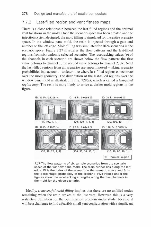
Design and manufacture of textile composites278
7.7.2 Last-filled region and vent fitness maps
There is a close relationship between the last-filled regions and the optimalvent locations in the mold. Once the scenario space has been created and theinjection system designed, the mold filling is simulated for the entire scenariospace. In the window pane mold, the resin is injected through a gate andnumber on the left edge. Mold filling was simulated for 1024 scenarios in thescenario space. Figure 7.27 illustrates the flow patterns and the last-filledregions from six randomly selected scenarios. The racetracking values (r) ofthe channels in each scenario are shown below the flow pattern: the firstvalue belongs to channel 1, the second value belongs to channel 2, etc. Nextthe last-filled regions from all scenarios are superimposed – taking scenarioprobabilities into account – to determine where last-filled regions concentrateover the mold geometry. The distribution of the last-filled regions over thewindow pane mold is illustrated in Fig. 728(a), which is called a last-filledregion map. The resin is more likely to arrive at darker mold regions in thefigure.
ID: 13 Pr: 0.1206 % ID: 15 Pr: 0.0559 % ID: 31 Pr: 0.0498 %
{1, 100, 1, 1, 1} {30, 100, 1, 1, 1} {30, 100, 10, 1, 1}
ID: 39 Pr: 0.1903 % ID: 92 Pr: 0.0443 % ID: 118 Pr: 0.0839 %
{30, 10, 25, 1, 1} {100, 30, 10, 10, 1} {10, 10, 80, 10, 1}
Terminal region
7.27 The flow patterns of six sample scenarios from the scenariospace of the window pane mold. The resin runner lies along the leftedge. ID is the index of the scenario in the scenario space and Pr isthe (percentage) probability of the scenario. Five values under thefigures show the racetracking strengths along the five channels inthe mold for the given scenario.
Ideally, a successful mold filling implies that there are no unfilled nodesremaining when the resin arrives at the last vent. However, this is a veryrestrictive definition for the optimization problem under study, because itwill be a challenge to find a feasibly small vent configuration with a significant

Modeling, optimization and control of resin flow 279
Pro
b,
st3:
0
.00
0.02
0.0
4 0.
08 0
.016
0.2
4 0.
31 0
.39
0.47
0.5
5 0.
63P
rob
:
0.03
0.0
6 0.
09 0
.13
0.01
7 0.
19 0
.23
Line source
(a)
(b)
7.28
(a)
Las
t-fi
lled
reg
ion
dis
trib
uti
on
in
win
do
w p
ane
mo
ld.
(b)
Co
rres
po
nd
ing
ven
t d
istr
ibu
tio
n p
lot
that
sh
ow
s th
em
erit
of
no
des
to
bec
om
e ve
nt
loca
tio
ns.

Design and manufacture of textile composites280
performance index. In order to relax this requirement, two tolerances areintroduced, based on the process physics: (i) dry spots that include fewernodes than a preset value at the time of formation are ignored, and (ii) inorder to drain air bubbles in the vicinity of a vent, a certain amount of resinis allowed to bleed after it arrives at the vent. The first tolerance is quantifiedin terms of nodes in a dry spot and the second tolerance is represented as adry spot-proof region of certain radius around a vent. Any mold fillingsimulation that satisfies both tolerances will be considered as successfullydrained (or successfully filled).
Owing to the introduction of the tolerances, a single scenario can besuccessfully drained by several vent configurations. Figure 7.29 illustratesthe mold filling contour plot for a certain scenario of a rectangular mold. Asingle gate at the center of the mold creates two last filled regions on theright and left sides of the mold. The air on the right side can be successfullydrained by a single vent at any of the nodes {265, 276, 277}. The air on theleft side can be drained by a single vent at any of the nodes {5, 6, 16, 17}.Hence, nodes {5, 6, 16, 17, 265, 276, 277} are possible vent configurationsin this scenario of the rectangular mold. Each scenario will give a differentset of nodes as the vent locations. A node may appear in many scenarios asa possible vent location. The cumulative probability of the scenarios it appearsin as a possible vent location, gives the fitness of that node to be a vent. Forthe window pane mold, the dry spot tolerance is taken as four nodes and theradius of the dry spot-free area around a vent is taken as the distance nodesbetween two. The vents are found for all scenarios and the fitness of thenodes to be vents are estimated and plotted in Fig. 7.28(b). The two contourplots in Fig. 7.28 are different, yet display similar morphological properties.The reason for the difference between the plots is the introduction of the dryspot tolerances. For example, Fig. 7.28(a) shows that dry spots are frequently
7.29 Nodes that can drain air successfully on the right and left sidesof the mold. Contour plot shows the flow front locations at severaltime steps.
6
5
17
16
138
Injectiongate
277
276
265

Modeling, optimization and control of resin flow 281
captured to the left of the two inserts in the mold. However, Fig. 7.28(b) doesnot suggest any vent in those two regions, because the sizes of the dry spotsare smaller than the dry spot tolerance. The vent distribution plot shows themerit of nodes becoming vents, hence it can be used as an elementary ventoptimization tool.
Although vent distribution plots display the merit of nodes becoming ventlocations, they are not sufficient to choose optimal vent locations, as theyexclude an important pieces of information: (i) each scenario is independentof other scenarios and (ii) each scenario requires all necessary vents. Even ifa single required vent is missing, a scenario will not be drained successfully.For example, for the scenario in Fig. 7.29, the possible vent locations are {5,6, 16, 17, 265, 276, 277}. However, it must be stated that there must be atleast two vents in the mold to drain this scenario: one vent from set {265,276, 277} and one vent from set {5, 6, 16, 17}. If either vent is missing, themold filling will not be successful in the process window represented by thisscenario. Vent distribution plots indicate the merit of individual nodes to bevents, but exclude the fact that certain nodes should act together in a ventconfiguration to be useful. Hence, a combinatorial search algorithm thatworks on a scenario basis is developed in the following section.
7.7.3 Combinatorial search (CS)
It has been shown by Gokce and Advani [44] that a vent configuration thatis created by merging two or more vent configurations includes all the scenariosfrom the individual vent configurations. Thus, in combinatorial search, superiorsmall vent configurations are found first and the optimal vent configurationis sought by merging the small vent configurations as explained below:
∑ Step I. For each scenario, the vent configurations with the smallest numberof vents that save the scenario are found. Note that a scenario is saved byseveral vent configurations owing to the dry spot tolerances. These smallvent configurations are called the elementary vent configurations (EVC)and are used as the building blocks of large vent configurations (i.e. ventconfigurations with a large number of vents) during the optimizationprocedure. The collection of all EVCs is called the EVC set E .
∑ Step II. The data from the previous step are rearranged to find the scenariossaved by each EVC. The cumulative probability of the scenarios saved byan EVC gives its success rate (performance index).
∑ Step III. EVCs with low success rates are eliminated from set e. Theremaining EVCs are grouped with respect to the number of vents theyinclude. ie is used to represent the group of elementary vent configurationswith i vents.
∑ Step IV. Note that there is a constraint on the number of vents, n. There are

Design and manufacture of textile composites282
various ways to combine elementary vent configurations from e that satisfythis constraint. For example, if four vents are allowed in a mold and theset e has vent configurations with one, two or three vents (e = 1e » 2e »3e), then all vent configurations that include four vents can be created asfollows:
4W = {1e ¥ 1e ¥ 1e ¥ 1e} » |1e ¥ 1e ¥ 2e} » {2e ¥ 2e} » {1e ¥ 3e}
7.10
∑ Step V. Instead of creating 4W at once, one may use the following incrementalprocedure, which is based on the underlying theory of the combinatorialsearch:
i = 1: 1W = 1e
i = 2: 2W = {1
W ¥ 1e} » {2e}
i = 3: 3W = {2
W ¥ 1e} » {1W ¥ 2e} » {3e}
i = n = 4: 4W = {3
W ¥ 1e} » |2W ¥ 2e} » {1W ¥ 3e}
At each step during the procedure, only superior vent configurations withhigh-performance indices (success rate) in iW are retained for the next step,reducing the computational cost significantly. In, this way, it is possible tointroduce minimum required performance as a second optimization stopcriterion, which will yield fewer vents with suffcient performance. Note thatoptimal vent configurations that include one, two or three vents are alsodetermined as a by-product of the procedure above.
7.7.4 Case study: the window pane mold
The combinatorial search is demonstrated on the window pane, a 1.6 ¥ 1.0m2 rectangular mold containing two inserts (Fig. 7.25). The mesh of thegeometry includes 175 nodes, 136 2D elements (quads) and 80 1D elements(bars). 1D elements are used to model racetracking channels. Top, bottomand right edges, and the perimeters of the inserts are identified as fiveracetracking channels. The racetracking conditions in each channel are forecastusing variations of the Weibull density function. The racetracking sets andassociated probability values are shown in Table 7.2. A scenario space with1024 scenarios is created to model the racetracking condition in the mold.The injection scheme is specified as constant flow rate through node 70 (x =0, y = 0.5 m) on the left edge, which is connected to a runner along the leftedge. The last-filled region map is illustrated in Fig. 7.28(a).
The number of vents is selected as four. Dry spots with three or fewernodes are tolerated and an area of 2-node radius around a vent is considereddry spot-proof. Set e is generated with 465 EVCs, which include one or two

Modeling, optimization and control of resin flow 283
vents, i.e. e = 1e » 2e. Using the incremental procedure at step V above, theoptimal vent configurations with one, two, three and four vents are foundconsecutively. The optimal vent configurations are also investigated using anexhaustive search. A vent candidate pool P is created from the nodes thatappeared in a last filled region, at least in one scenario. Vent configurationsare created by taking Cartesian products of P. When the computational costbecomes prohibitive for large vent configurations, the candidate pool is sampledevenly (geometrically) to reduce the pool size. The ES conducted using adownsized candidate pool is called partial exhaustive search (partial ES).While ES provides the optimum solution, a partial ES may not provide theoptimum solution, but will indicate near-optimal solutions. The results of CSand ES are compared for accuracy and efficiency. The computational cost isreported in terms of the duration of the optimization process. Gateway 2000computers with Pentium 4 1600 MHz processors and 256MB RAM wereused for this study. The results for CS and (partial) ES are listed in Table 7.3.The results for the 3-vent and 4-vent cases are illustrated in Fig. 7.30. In eachcase, all nodes that appeared as vent locations are shown on the figure. Theperformance index of the CS result is shown with a pie chart on each figure.The computational cost comparison between the CS and ES (or partial ES)is illustrated with a bar plot. CS results are as accurate as ES results andbetter than partial ES results. Computational savings are 57%, 91%, 99%and 97% for 1-vent, 2-vent, 3-vent and 4-vent optimization, respectively.
Table 7.3 CS and ES optimization results for window pane mold. Performanceindex is the cumulative probability of the scenarios that are drained by V *
Optimization Optimal vent Performance Computationalmethod configurationa, V * index, f(V *) cost (s)
(node numbers)
Creation of set e – – 69
CS 118 27.6% 69ES 118 27.6% 162
CS 107 117 48.2% 209ES 107 117 48.2% 2,439
CS 57 107 117 69.0% 301ES 57 107 117 69.0% 44,570
CS 57 106 118 168 87.9% 1,364Partial ES 57 107 117 169 87.3% 51,165
ax and y coordinates of the nodes are as follows (in m): 57 (1.4, 0.0), 106 (1.3, 0.5),107 (1.3, 0.6), 117 (1.6, 0.4), 118 (1.6, 0.5), 168 (1.4, 0.9), 169 (1.4, 1.0).
As a benchmark, an intuitive vent design, illustrated in Fig. 7.31, wastested in the scenario space. The success rate was only 28% as compared to69% with the optimal 3-vent vent configuration.

Design and manufacture of textile composites284
CS
P. I
nd
ex
CS
ES
107
117
CS
P. I
nd
ex
CS
P. E
S
57C
S r
esu
lt(P
) E
S r
esu
lt
107
106
169
168
118
117
57
7.30
Op
tim
al 3
-ven
t ( l
eft)
an
d 4
-ven
t ( r
igh
t) v
ent
con
fig
ura
tio
ns
in t
he
win
do
w p
ane
mo
ld a
s fo
un
d b
y co
mb
inat
ori
alse
arch
(C
S)
and
exh
aust
ive
sear
ch (
ES
). S
ince
eac
h o
pti
miz
atio
n m
eth
od
ret
urn
ed d
iffe
ren
t re
sult
s, v
ent
loca
tio
ns
are
sho
wn
by
dif
fere
nt
mar
kers
, as
illu
stra
ted
in
th
e le
gen
d.

Modeling, optimization and control of resin flow 285
Mold symmetry and scenario space
The window pane mold has many symmetric features: the geometry, injectionconditions, density function and the racetracking sets of symmetric channels.Consequently, last-filled region and vent fitness maps are also symmetric.Therefore:
∑ Two vent configurations that are symmetries of each other will yield thesame results.
∑ It is erroneous to investigate a section of the geometry only, since severalscenarios in the scenario space are not symmetric owing to differentracetracking conditions along the symmetric channels. Yet, several scenariosare symmetric with respect to each other. Two scenarios are called symmetricif the resin flow pattern of one is a symmetry of the flow pattern in theother across an axis. The size of the scenario space can be reduced byeliminating one of the symmetric scenario groups. Later, the optimal ventconfiguration for the reduced scenario space can be mirrored acrosssymmetry axes to create the optimal vent configuration for the entirescenario space.
7.8 Conclusion
Resin flow through textile preforms in the mold cavity was modeled insection 7.2 using Darcy’s law. Liquid injection molding simulation (LIMS),which was used to simulate resin flow in the mold cavity, was introduced insection 7.3. Its features and utilization in design, optimization and controlstudies were presented. The branch and bound search was adapted to gatelocation optimization in section 7.4 and its application was demonstratedwith a case study. Section 7.5 introduced the disturbances associated withthe mold filling process. Racetracking was identified as the key disturbanceand it was shown with a case study that it is not repeatable. Active andpassive control methods that enable successful mold filling in the presence
Vent
7.31 The vent configuration used as a benchmark to evaluate theperformance of the optimization algorithm Combinatorial Search.
Design and manufacture of textile composites286
of racetracking were proposed in sections 7.6 and 7.7, respectively. In activecontrol, which was exemplified by simulation-based liquid injection control(SLIC), the resin flow is redirected by varying the injection conditions at theinjection gates. In passive control, racetracking conditions were modeledprobabilistically and a sufficient number of vents are placed at locationswhere resin is more likely to arrive last. The approaches and procedures tocreate these strategies were presented with pedagogic examples.
7.9 Outlook
The knowledge base about LCM processes is growing every day. Severaltools and methodologies that address modeling, design, optimization andcontrol issues are available or under development. Ultimately, the aim is todevelop the LCM technology to the extent that simple, high-volume partswill be manufactured quickly, and large, complex and low volume parts willbe manufactured successfully. A maximum level of automation is desirable,especially for the former group. Since automation makes the manufacturingsteps repeatable, the average quality of the parts will increase. Automationalso cuts down the labor costs and decreases the health hazards by decreasingthe exposure of the workers to the resin fumes and preform soot. Reducingthe reject rate is a prime goal in all cases.
Further research and development is necessary to bring LCM processes totheir full potential. The work presented in this chapter spans several importantissues in mold filling. Some of the future research directions are presentedbelow.
7.9.1 Multiple gate optimization
This topic is rarely addressed by the researchers, possibly because of theextensive computational effort required. There is a permutational relationshipbetween the number of the gates and the problem size: in a mold with Nnodes, there are N possibilities for the first gate, N(N – 1) possibilities for thesecond gate, etc. An optimally designed multi-injection system can reducethe fill time significantly and hence the need to explore optimization methodsthat can address this issue effectively.
7.9.2 Optimal placement of flow enhancement media
In LCM processes such as VARTM (or vacuum infusion), a flow enhancementmedium is placed on the entire surface of the preform to distribute the resinquickly. However, this method is not applicable when there are mold regionsthat are inaccessible for the flow enhancement medium or the vacuum line asshown in Fig. 7.32. Also, if the mold geometry is complex and includes

Modeling, optimization and control of resin flow 287
inserts or ribs, such a design may fail to fill the mold successfully. Therefore,the flow enhancement medium needs to be designed optimally in these casesin order to increase the efficiency of the mold filling operation.
7.9.3 Use of manufacturing data for racetrackingforecast
In section 7.7, a generic density function was used to forecast racetrackingin the racetracking channels for illustration purposes. In actual applications,the racetracking forecast must capture the manufacturing conditions, whichare assumed to be stable. Statistics from the manufacturing floor and equipment,material and processing tolerances must be incorporated into the racetrackingforecast. Even if it is not possible to capture the actual case exactly, a sufficientlyaccurate racetracking forecast will be very useful to test various designs inthe simulation environment.
7.9.4 Feasible target flow pattern selection in set point-based active control
Set point-based feedback controllers generate control inputs based on thetracking error between the target flow pattern and the actual flow pattern. Aflow pattern strongly depends on the permeability field in the mold cavity.Given a permeability field and a gate configuration, there is a finite range offlow patterns that can be created by modifying the injection conditions at thegates, which is called the reachable set. For a controller to be successful inminimizing the tracking error, the target flow pattern must belong to this set.Therefore, it is crucial to predict the reachable set in the presence of disturbances
7.32 A composite part geometry that does not allow the placement offlow enhancement media over the entire geometry.
Flow enhancement media (number of plies = 2, 1 or 0)
Prefabricatedrib structure
Injection line
Preform
Vent line

Design and manufacture of textile composites288
and select a feasible target flow pattern. Multiple target flow patterns can beselected as needed depending on the racetracking forecast.
7.10 Acknowledgements
The financial support, provided by the Office of Naval Research (ONR)under Grant N000l4-97-C-0415 for the Advanced Materials IntelligentProcessing Center at the University of Delaware, made the work presented inthis chapter possible. The invaluable contributions of Dr Pavel Simacek, DrKuang-Ting Hsiao and Mathieu Devillard to this chapter are kindly appreciated.
7.11 References
1. Advani S.G. and Sozer M.E., Process Modeling in Composites Manufacturing. MarcelDekker, New York, 2003.
2. Advani S.G., Resin transfer molding in Flow and Rheology in Polymeric CompositesManufacturing, pages 465–516. Elsevier Publishers, Amsterdam, 1994.
3. Rosato D.V. and Lee (ed.) S.M., Polymeric Matrix Composites in InternationalEncyclopedia of Composites, volume 3, pages 148–181. VCH Publishers, Inc., NewYork, 1990.
4. Schwartz M.M., Composite Materials Handbook. McGraw Hill, New York, 1992.5. Gokce A., Modeling of flow continuum and optimal design of control-oriented
injection systems in liquid composite molding processes. PhD thesis, University ofDelaware, 2003.
6. Bickerton S., Modeling and control of flow during impregnation of heterogeneousporous media, with application to composite mold filling processes. PhD thesis,University of Delaware, Spring 1999.
7. Stadtfeld H.C., Experimental validation of impregnation schemes with control strategiesin liquid composite molding processes. Master’s thesis, University of Delaware, 2000.
8. Kueh S.R.M., Fiber optic flow monitoring system and methodology for sensorplacement to identify flow disturbances in liquid composite molding. PhD thesis,University of Delaware, Summer 2001.
9. Kozeny J., Sitzungsberichte Abt IIa. Wiener Akademie der Wissenschaft, 1927.10. Carman P.C., Fluid Flow Through Granular Beds. Transactions 15, Institution of
Chemical Engineers, 150–166, 1937.11. Dave R., Kardos J.L. and Duducovic M.P., A model for resin flow during composite
processing. part 2: Numerical analysis for unidirectional graphite/epoxy laminates.Polymer Composites, 8(2), 1987.
12. Lam R.C. and Kardos J.L., The permeability and compressibility of aligned andcross-plied carbon fiber beds during processing of composites. In Proceedings ofANTEC, SPE, New York, May 1989.
13. Bruschke M.V., A predictive model for permeability and non-isothermal flow ofviscous and shear-thinning fluids in anisotropic fibrous media. PhD thesis, Universityof Delaware, 1992.
14. Chiemlewski C., Petty C.A. and Jeyaraman K., Crossflow permeation of viscous andviscoelastic liquids in cylinder arrays. In Proceedings of the American Society forComposites Fifth Technical Conference, East Lansing, June 1990.

Modeling, optimization and control of resin flow 289
15. Simacek P. and Advani S.G., Permeability model for woven fabrics. PolymerComposites, 17(6): 887–899, December 1996.
16. Chang W. and Kikuchi N., Analysis of non-isothermal mold filling process in resintransfer molding (RTM) and structural reaction injection molding (SRIM).Computational Mechanics, 16(1): 22–35, 1995.
17. Lee C.K., Sun C.C. and Mei C.C., Computation of permeability and dispersivities ofsolute or heat in periodic porous media. International Journal of Heat and MassTransfer, 39(4): 661–676, 1996.
18. Dimitrovova Z. and Faria L., Finite element modeling of the resin transfer moldingprocess based on homogenization techniques. Computers and Structures, 76(1):379–397, 2000.
19. Koponen A., Kataja M. and Timonen J., Statistical physics, plasmas, fluids, andrelated interdisciplinary topics. Physical Review E, 56(3): 3319–3320, 1997.
20. Spaid M. and Phelan F., Modeling void formation dynamics in fibrous porous mediawith the lattice boltzman method. Composites Part A, 29 (7): 749–755, 1998.
21. Gokce A. and Advani S.G., Permeability estimation with the method of cells. Journalof Composite Materials, 35(8): 713–728, 2001.
22. Nedanov P., Permeability characterization of fibrous porous media. Master’s thesis,University of Delaware, 2002.
23. Gebart B.R., Permeability of unidirectional reinforcements for RTM. Journal ofComposite Materials, 26(8): 1100–1133, 1992.
24. Verheus A.S. and Peeters J.H., A. The role of reinforcement permeability in resintransfer molding. Composites Manufacturing, 4(1): 33–38, 1993.
25. Parnas R.S. and Salem A.J. A comparison of the unidirectional and radial in-planeflow of fluids through woven composite reinforcements. Polymer Composites, 14(5):383–394, 1993.
26. Ferland P., Guittard D. and Trochu F., Concurrent methods for permeabilitymeasurement in resin transfer molding. Polymer Composites, 17(1):149–158, 1996.
27. Wang J.T., Wu C.H. and Lee L.J., In-plane permeability measurement and analysisin liquid composite molding. Polymer Composites, 15(4): 278–288, 1994.
28. Weitzenbock J.R., Shenoi R. A. and Wilson P.A., Measurement of three-dimensionalpermeability. Composites Part A, 29(1–2): 159–169, 1998.
29. Bruschke M.V. and Advani S.G., A finite element/control volume approach to moldfilling in anisotropic porous media. Polymer Composites, 11: 398–405, 1990.
30. Bruschke M.V. and Advani S.G., A numerical approach to model non-isothermalviscous flow through fibrous media with free surfaces. International Journal forNumerical Methods in Fluids, 19: 575–603, 1994.
31. Lee L.J., Young W.B. and Lin R.J., Mold filling and cure modeling of RTM andSRIM processes. Composite Structures, 27(1–2): 109–120, 1994.
32. Tredoux L. and Westhuizen J., Van der. Development of a numerical code thatsimulates combined heat transfer, resin flow and compaction during compositeprocessing. Composites Manufacturing, 6(2): 85–92, 1995.
33. Fracchia C.A., Castro J. and Tucker III C.L., A finite element/control volume simulationof resin transfer molding. In Proceedings of the ASC 4th Annual Technical Conference,Santa Monica, October 1995.
34. Young W.-B., Consolidation and cure simulation for laminated composites. PolymerComposites, 17(1): 142–148, 1996.
35. Liu X.-L., Isothermal flow simulation of liquid composite molding. Composites PartA: Applied Science and Manufacturing, 31(12): 1295–1302, Dec 2000.

Design and manufacture of textile composites290
36. Simacek P., Sozer E.M. and Advani S.G., User Manual for DRAPE 1.1 and LIMS4.0 Liquid Injection Molding Simulation, Technical Report UD-CCM 98-01. Centerfor Composite Materials, University of Delaware, Newark, DE, 1998.
37. The Mathworks, Inc., http://www.mathworks.com. Learning MATLAB.38. Mathur R., Advani S.G. and Fink B.K., Use of genetic algorithms to optimize gate
and vent locations for the resin transfer molding process. Polymer Composites, 20:167–178, 1999.
39. Gokce A., Hsiao K.-T. and Advani S.G., Branch and bound search to optimizeinjection gate locations in liquid composite molding processes. Composites: Part A,33: 1263–1272, 2002.
40. Papalambros P.Y. and Wilde D.E., Principles of Optimal Design: Modeling andComputation. Cambridge University Press, Cambridge, 1988.
41. Rao S.S., Optimization: Theory and Applications. Wiley Eastern Limited, New Delhi,1979.
42. Parker R.G. and Rardin R.L., Discrete Optimization. Academic Press Inc., San Diego,1988.
43. Horst R. and Tuy H., Global Optimization: Deterministic Approaches. Springer-Verlag, Berlin, 3rd edition, 1996.
44. Gokce A. and Advani S.G., Combinatorial search to optimize vent locations in thepresence of disturbances in liquid composite molding processes. Materials andManufacturing Processes, 18(2): 261–285, 2003.
45. Bickerton S. and Advani S.G., Characterization of corner and edge permeabilitiesduring mold filling in resin transfer molding. In Proceedings of the ASME AMD-MDSummer Meeting, volume 56, pages 143–150, Los Angeles, CA, June 1995.
46. Bickerton S. and Advani S.G., Characterization of racetracking in liquid compositemolding processes. Composites Science and Technology, 59: 2215–2229, 1999.
47. Han K., Wu C.H. and Lee L.J., Characterization and simulation of resin transfermolding – racetracking and dry spot formation. In Proceedings of Ninth AnnualASM-ESD Advanced Composite Conference, Michigan, 1993.
48. Leek R., Carpenter G., Donnellan T. and Phelan F., Simulation of edge flow effectsin resin transfer molding. In Proceedings of the 25th International SAMPE TechnicalConference, pages 233–245, Philadelphia, Oct 1993.
49. Ni J., Zhao Y., Lee L.J. and Nakamura S., Analysis of two regional flow in liquidcomposite molding. Polymer Composites, 18(2): 254–269, 1997.
50. Sheard J., Senft V., Mantell S.C. and Vogel J.H., Determination of corner and edgepermeability in resin transfer molding. Polymer Composites, 19(1): 96–105, 1998.
51. Hammami A., Gauvin R. and Trochu F., Modelling the edge effect in liquid compositemolding. Composites Part A: Applied Science and Manufacturing, 29(5–6): 603–609, 1998.
52. Bickerton S. and Advani S.G., Characterization of racetracking in liquid compositemolding processes. Composites Science and Technology, 59: 2215–2229, 1999.
53. Chaneske J., Jayaraman K., Norman D. and Robertson R., Effects of preformarchitecture on racetracking in liquid molding. In Proceedings of International SAMPESymposium and Exhibition, pages 954–966, Long Beach, CA, May 2000.
54. Tadmor Z. and Costas G.G., Principles of Polymer Processing. John Wiley and Sons,New York, 1979.
55. Data compiled and evaluated by Parnas R.S. and Flynn K.M., NIST Data Base onReinforcement Permeability Values, Version 1.0. NIST Std. Ref. Database 63.
56. Devillard M., Hsiao K.-T., Gokce A. and Advani S.G., On-line characterization of

Modeling, optimization and control of resin flow 291
bulk permeability and race-tracking during the filling stage in resin transfer moldingprocess. In 34th International SAMPE Technical Conference, Baltimore, November2002.
57. Demirci H.H. and Coulter J.P., Neural network based control of molding processes.Journal of Materials Processing and Manufacturing Science, 2: 335–354, 1994.
58. Demirci H.H. and Coulter J.P., Control of flow progression during molding processes.Journal of Materials Processing and Manufacturing Science, 3(4): 409–425, 1995.
59. Demirci H.H., Coulter J.P. and Guceri S.I., Numerical and experimental investigationof neural network-based intelligent control of molding processes. Journal ofManufacturing Science and Engineering, Transactions of the ASME, 119(1): 88–94,1997.
60. Berker B., Barooah P., Yoon M.K. and Sun J.Q., Sensor based modeling and controlof fluid flow in resin transfer molding. Journal of Materials Processing andManufacturing Science, 7(2): 195–214, 1998.
61. Nielsen D. and Pitchumani R., Real time model-predictive control of preformpermeation in liquid composite molding processes. In Proceedings of the ASMENational Heat Conference, Pittsburgh, August 2000.
62. Sozer E.M., Bickerton S. and Advani S.G., Modeling and control of liquid compositemold filling process. In Proceedings of Flow Processes in Composite Materials(FPCM), Plymouth, UK, pages 109–124, July 1999.
63. Hsiao K.-T., Devillard M. and Advani S.G., Streamlined intelligent rtm processing:From design to automation. In Proceedings of 47th International SAMPE Symposiumand Exhibition, volume 47, pages 454–465, Long Beach, CA, May 2002.
64. Westphal L.C., Sourcebook of Control Systems Engineering. Chapman & Hall, London,1992.
65. Kazimierz M., Zbigniew N. and Malgorzata P., Modelling and Optimization ofDistributed Parameter Systems. Chapman & Hall, London, 1996.
66. Tzou H.S. and Bergman L.A., Dynamics and Control of Distributed Systems. CambridgeUniversity Press, Cambridge, 1998.
67. Tzafestas S.G., Distributed Parameter Control Systems. Pergamon Press, Oxford,1982.
68. Avdonin S.A. and Ivanov S.A., The Method of Moments in Controllability Problems,for Distributed Parameter Systems. Cambridge University Press, Cambridge, 1995.
69. Grinberg A.S., Lototskii V.A. and Shklyar B., Sh. Controllability and observabilityof dynamic systems. Automation and Remote Control (English translation of Avtomatikai Telemekhanika), 52(1): 1–16, June 1991.
70. Cao Y., Gunzburger M. and Turner J., Controllability of systems governed by parabolicdifferential equations. Journal of Mathematical Analysis and Applications, 215(1):174–189, Nov. 1997.
71. Gokce A. and Advani S.G., Gate effectiveness in controlling resin advance in liquidcomposite molding processes. Journal of Manufacturing Science and Engineering,125(3): 548–555, 2003.

292
8.1 Introduction
Textile composites are used typically because of their high strength-to-weightand stiffness-to-weight ratios. In order to exploit these properties it is essentialto have a good understanding of their behaviour under load, beginning withthe capability to model their stiffness and later consider their strength viasuitable failure criteria. It is normal to assume that composites (especiallyreinforced thermosets) are linear elastic up to the point of failure, althoughthere is some evidence that even thermoset matrix materials can yield inshear. Moreover, there is now increasing interest not just in the modelling ofdamage onset but also the degradation in properties of a structure as damageprogresses. However, in order to be able to reach that stage, an accurateunderstanding of the structure’s elastic behaviour must be established. Hencethis chapter starts with a description of elastic behaviour, from simpleapproaches based on micromechanics and classical laminate theory to moresophisticated analyses developed specifically for textile composites. This isfollowed by a description of failure behaviour, with particular emphasis onimpact loading.
8.2 Elastic behaviour
The application of elasticity to composite materials (even idealised ones, letalone those with the complex fibre architecture of textile-reinforced composites)is an extremely complex area, and any summary of this field in a few pagesneeds to be accompanied by some strong notes of caution. The first of theseis that the ensuing description is only a flavour of the basic theory, and thereader should have no difficulty in locating a number of texts covering thisbasic material (and its underlying assumptions and limitations) in more detail.For a more in-depth treatment of some aspects, the reader is referred to thevery detailed text by Bogdanovitch and Pastore1, and is encouraged to review thelatest literature in the field, some of which is referenced in the present chapter.
8Mechanical properties of textile composites
I A J O N E S, University of Nottingham, UK andA K P I C K E T T, Cranfield University, UK

Mechanical properties of textile composites 293
The second note of caution is that there are many variants on the notationand definitions used within the theory, with differences ranging from thesuperficial (the choice of symbols used to represent the various quantities) tothe more fundamental (the use of matrices and contracted notation, cf. tensorialnotation; mathematical, cf. engineering definition of shear strains). It is thereforevital to ensure that the correct notation and conventions are used beforemaking use of any formula or computer program. The notation used here isessentially that of of Hull and Clyne2 and of Jones3, with some minor variations.A summary of the notation, and a more extended presentation of the materialin section 8.2.1 is available in Appendix A of Owen et al4.
8.2.1 Fundamentals: orthotropic solids
In order to understand the behaviour of textile reinforced composites it isnecessary first to study the concepts of anisotropic and orthotropic behaviour,and to introduce relevant concepts from laminate analysis. Viewed at amicroscopic level, textile composites (irrespective of their fibre architecture)are assembled from bundles of parallel fibres embedded in (and assumed tobe rigidly bonded to) a matrix material that is usually polymeric and has amuch lower modulus than the fibres, and is usually assumed to be homogeneousand isotropic (i.e. properties constant throughout irrespective of position ororientation). This structure will clearly have stiffness and strength propertieswhich are much greater in the direction of the fibre than in any perpendiculardirection. Figure 8.1 shows an idealisation of this structure, where the symmetryof the structure is apparent, and enables us to simplify our treatment of theelastic behaviour from the general case of true anisotropy (material propertiesdifferent in all directions with no symmetry).
8.1 Schematic diagram of fibre-reinforced composite as anorthotropic solid showing three planes of symmetry.

Design and manufacture of textile composites294
The elastic behaviour (i.e. the relationship between stresses and strains inthe three principal directions) of a material possessing three such planes ofsymmetry is characterised by the orthotropic constitutive model. This isfully defined by three elastic moduli E1, E2 and E3, three independent Poisson’sratios n12, n23 and n31 and three shear moduli G12, G23 and G31. Three furtherPoisson’s ratios are related to the aforementioned moduli and Poisson’s ratios:
n n21 122
1 =
EE
; n n32 233
2 =
EE
; n n13 311
3 =
EE
8.1
The elastic behaviour may be expressed via Hooke’s law for orthotropicmaterials:
e1 = 11E
(s1 – n12s2 – n13s3)
e2 = 12E
(s2 – n21s1 – n23s3)
e3 = 13E
(s3 – n31s1 – n32s2)
g t12
12
12 =
G g t
2323
23 =
G g t
1313
13 =
G8.2
This is a generalisation of the isotropic three-dimensional (3D) expressionof Hooke’s law, one of the first mathematical relationships to which studentsof solid mechanics are exposed. In practice we are generally interested in athin layer or lamina of material (or, eventually, an assembly of them); in thiscase it can usually be assumed that through-thickness stress (defined to bes3) is negligible and the through-thickness strain (e3) is unimportant. Equation8.2 can therefore be simplified to express the strains within the 1–2 plane interms of the stresses in that plane:
3
2
1
8.2 Orthotropic solid loaded along its axis displays no tension-shearcoupling.

Mechanical properties of textile composites 295
e s n s11
1 12 2 = 1 ( – )E
e s n s22
2 21 1 = 1 ( – )E
g t12
12
12 =
G8.3
These relationships may be expressed more conveniently in matrix form:
eeg
n
n
t
sss
sst
1
2
12
1
12
1
21
2 2
12
1
2
12
11 12
12 22
66
1
2
12
=
1 – 0
– 1 0
0 0 1
=00
0 0
ÏÌÔ
ÓÔ
¸˝Ô
Ô
È
Î
ÍÍÍÍÍÍ
˘
˚
˙˙˙˙˙˙
ÏÌÔ
ÓÔ
¸˝Ô
Ô
È
ÎÍÍ
˘
˚˙˙
ÏÌÔ
ÓÔ
¸˝Ô
Ô
E E
E E
S SS S
S
or {e} = [S]{sssss} 8.4
where S11, etc., are elements of the on-axis compliance matrix [S] of alamina. For elastic behaviour the compliance matrix must be symmetric, sothat n12/E1 = n21/E2 which follows on from eqn 8.1. Therefore only fourindependent constants (E1, E2, G12 and either of the Poisson’s ratios) areneeded to define the in-plane elastic behaviour of a lamina. Note the presenceof the zeros in the matrices in eqn 8.4; these mean that the material does notdistort in shear when stretched in the on-axis direction (Fig. 8.2).
This behaviour is a direct consequence of the symmetry noted in Fig. 8.1.Sometimes it is preferable instead to express stresses in terms of strains:
s
s
t
n nnn n
nn n n n
e
e
g
1
2
12
1
12 21
12 2
12 21
21 1
12 21
1
12 21
12
1
2
12
11 12
=
1– 1–0
1– 1–0
0 0
=
0Ï
Ì
ÔÔÔ
Ó
ÔÔÔ
¸
˝
ÔÔÔ
˛
ÔÔÔ
È
Î
ÍÍÍÍÍÍÍ
˘
˚
˙˙˙˙˙˙˙
Ï
Ì
ÔÔÔ
Ó
ÔÔÔ
¸
˝
ÔÔÔ
˛
ÔÔÔ
E E
E E
G
Q Q
Q1212 22
66
1
2
12
0
0 0
Q
Q
È
Î
ÍÍÍÍÍÍ
˘
˚
˙˙˙˙˙˙
Ï
Ì
ÔÔÔ
Ó
ÔÔÔ
¸
˝
ÔÔÔ
˛
ÔÔÔ
e
e
g
or {sssss} = [Q]{eeeee} 8.5
where Q11, etc., are elements of the on-axis ‘reduced’ (plane stress) stiffnessmatrix [Q] of the lamina, and [Q] ∫ [S]–1. Note that these reduced stiffnessterms are not equal to the corresponding terms in the 3D stiffness matrix forthe material. In section 8.2.3 we shall return to the manipulation of theseelastic stiffnesses and compliances, but it is useful at the present stage toconsider how values for the above moduli and Poisson’s ratios can be obtained.

Design and manufacture of textile composites296
8.2.2 Obtaining the unidirectional properties: testing andmicromechanics
The above analysis assumed the availability of the unidirectional bulk propertiesof the composite material, and later sections will assume knowledge of thelocal properties of the impregnated fibre bundles (tows) which (along withthe regions of pure resin) constitute textile reinforced composite materials.However, obtaining these properties is problematic. It must be realised thatcomposite materials differ in one vital respect from conventional engineeringmaterials such as metals: they do not generally exist as an entity until themanufacture of the component from which they are made. In other words,they are not (with some exceptions) produced by melting or machining stockmaterial but are created from resin and fibre (or a mixture of the fibre and anuncured resin or thermoplastic matrix) at the time of moulding, and theirproperties depend heavily upon the manufacturing processing conditions.There are two main approaches: experimental measurement using standardtesting procedures, and theoretical prediction from the properties of theconstituent materials (fibre and matrix). By far the best way of obtainingmaterial properties for design purposes is to perform tests on statisticallylarge samples of materials. Such testing is time consuming and the resultingproperties often constitute closely guarded proprietary data. It is importantthat such tests are conducted to recognised standards.
Measurement of unidirectional and laminate properties: testing methods
Experimental testing may be applied both to the purely unidirectional materialand to the finished laminate. A detailed discussion of testing procedures isinappropriate here; instead, reference is made to the various standards in usewhich define various methods of obtaining the required properties. In particular,BS2782-10 covers various aspects of testing of reinforced plastics (notablymethod 10035, which covers tensile testing, and 10056, which covers flexuraltesting). Standardised test methods for unidirectional materials are also available(for example, ISO 527-5:19977, which covers the testing of unidirectionalreinforced plastics). Experimental determination of shear properties isproblematic; one widely used method is the Iosipescu test embodied in ASTMstandard D53798, which involves the testing of small, vee-notched specimensloaded within a special frame that subjects them to pure shear within thegauge region. Shear strength properties are easily obtained from the maximumload measured; elastic properties may be determined via the use of a ±45∞strain gauge bonded onto the gauge region of the specimen.

Mechanical properties of textile composites 297
Prediction of unidirectional properties: micromechanics
Instead of physically constructing a unidirectional material or a laminate andperforming tests, an alternative approach is to predict the unidirectionalbehaviour of the composite from the properties of its constituent materials,namely its fibre and matrix. This approach is clearly better than nothing, buthas some important limitations:
∑ The spatial distribution of the fibres within the matrix is unknown.∑ Wet-out and interfacial bonding are normally assumed to be perfect but
are unlikely to be so in practice (there may, for instance, be dry regionswithin each tow of fibres).
∑ While the on-axis elastic behaviour of composites is fibre-dominated andrelatively easy to predict, the transverse and shear behaviours result fromcomplex stress distributions within the composite and are much less easyto predict theoretically.
The prediction of composite properties from those of the fibre and matrixis one example of the discipline known as micromechanics, and a number oftheoretical and semi-empirical models exist. The simplest is known as the‘rule of mixtures’, and probably the most commonly used is a refinement ofthat method known as the Halpin–Tsai equations, although more sophisticatedapproaches exist such as the composite cylinder assemblage approach, whichcan take account of anisotropic properties in the fibres themselves.
Rule of mixtures
The rule-of-mixtures approach3 is applicable particularly to the determinationof the longitudinal modulus of a unidirectional composite and of its majorPoisson’s ratio; its application to transverse and shear moduli gives lessaccurate results. In the case of the longitudinal modulus, the assumption ismade that the strain along a two-dimensional (3D) block of material (Fig.8.3) is uniform (the iso-strain assumption explored in more detail in section8.2.3) and that no transverse stresses are present. For a given value of strain,
Fibres Matrix
Longitudinal strain e
Cross-sectional area A
Total force= AVfeEf + AVmeEm= Ae[EfVf + Em(1 – Vf)]
8.3 Rule of mixtures approach to determine longitudinal modulus.

Design and manufacture of textile composites298
the loads carried by the fibre and matrix components will be proportionalboth to their moduli and to the cross-sectional area of the fibre and matrix,with the respective areas being proportional to the fibre and matrix volumefractions; in other words, the fibres and matrix are assumed to be elasticbodies (springs) acting in parallel. This leads to the following expression forlongitudinal modulus E1:
E1 = EfVf + EmVm = EfVf + Em (1 – Vf) 8.6
where it is assumed that there is no void content in the composite, and whereEf and Em are respectively the elastic moduli of the fibre and matrix, and Vf
and Vm ∫ 1 – Vf are respectively the volume fractions of the fibre and matrix.A slightly less trivial derivation leads to a very similar expression for themajor Poisson’s ratio n12 (which in a UD material can be assumed to beidentical to n13):
n12 = nfVf + nm (1 – Vf) 8.7
Both these expressions are found to give answers of good accuracy. Bycontrast, the application of the rule of mixtures to the transverse elasticproperties requires the assumption that the fibres and matrix are elastic bodiesin series (requiring the iso-stress assumption, again explained in section8.2.3); this is very much a simplification since the true arrangement is three-dimensional and is a combination of series and parallel behaviour. The resultingexpression for E2 (∫ E3) is rather inaccurate but is presented below forcompleteness:
1 = 1 + 1 (1 – )2 f
fm
fE EV
EV 8.8
Similar arguments apply to the shear moduli (for which both the series andparallel assumptions give poor results), but these will not be pursued furtherhere.
The Halpin–Tsai equations
The Halpin–Tsai equations9, 10 are effectively a refinement and generalisationof the rule of mixtures. Indeed, for the longitudinal modulus E1 and majorPoisson’s ratio n12 the rule of mixtures is used directly via eqns 8.6 and 8.7.The basis of the approach for the transverse and shear moduli is to assumeintermediate situations between the extremes of the series and parallel modelsto which the rule of mixtures is restricted. For these moduli, the form of theequation is as follows:
MM
VVm
f
f =
1 + 1 –
xhh 8.9a

Mechanical properties of textile composites 299
where: hx
= / ) – 1
( / ) + f m
f m
(M MM M
8.9b
in which:M = E2, G12 and G23 for compositeMf = fibre property Ef or Gf
Mm = matrix property Em or Gm
Vf = fibre volume fraction(proportion of composite by volume)
x is a constant relating to the way the load is shared between fibre andmatrix within the model; its value must lie between the extremes of x = 0 (inwhich case eqn 8.9(a) simplifies to the series model similar to eqn 8.8) andx = • (when eqn 8.9(a) simplifies to the parallel model similar to eqn 8.6).For low fibre volume fractions (up to 65%) x may be assumed to be 2 and 1respectively for the calculation of E2 (and E3) and G12 (and G13). For highervolume fractions (as may be encountered within densely packed fibre tows),correction factors may be applied. For the calculation of G23 a simple valueof x is insufficient so a formula is required in any case. The three formulaefor x are therefore9:
x @ 2 + 40 f10V for calculation of E2 and E3
x @ 1 + 40 f10V for calculation of G12 and G13
x n 14 – 3 m
@ for calculation of G23 8.10
Halpin10 states that the Poisson’s ratio n23 in the transverse plane may becalculated approximately from the relevant direct and shear moduli using thefollowing relationship:
n 232
23 1 –@ E
G8.11
Hashin’s composite cylinder assemblage model
Although the above formulae are widely quoted and used, no publishedresults have been found that evaluate their accuracy for use with fibres (suchas carbon or aramid) whose properties are themselves anisotropic. One modelwhich does take account of fibre anisotropy is Hashin’s composite cylinderassemblage (CCA) model11, 12. This gives closed form expressions for E1,G12, the bulk modulus and n12, and upper and lower bounds on the transversemoduli. The expressions are rather lengthy, and the interested reader is advisedto refer to Hashin11 or the appendix of Naik and Shembekar13.

Design and manufacture of textile composites300
8.2.3 Off-axis behaviour and laminates
The analysis in section 8.2.1, and the properties discussed in section 8.2.2,relate purely to material where the fibres all lie with their axes in the samedirection, defined to be the 1-direction of the material’s local coordinatesystem. Practical textile reinforced composites can of course have very complexfibre architectures, so this discussion will concentrate next upon one of thesimplest of such structures, a planar plate constructed using layers of non-crimp textile reinforcement. The analysis which follows may be found inalmost any text on composite materials, such as those by Hull and Clyne2
and Jones3. A global Cartesian coordinate system provides a frame of referencefor definition of stresses and strains in each layer, and for the overall loadson and deformations of the plate: the x and y axes are coplanar with the plateand the z axis is perpendicular to the plate and measured from its mid-surface. Consider a thin lamina within such a structure, with its fibre axesorientated at angle q to the global x direction. The stresses present in thatlamina may be expressed in terms of the in-plane strains which that laminaundergoes:
sst
eeg
x
y
xy
x
y
xy
Q Q Q
Q Q Q
Q Q Q
Ï
ÌÔ
ÓÔ
¸
˝Ô
˛Ô
È
Î
ÍÍÍ
˘
˚
˙˙˙
Ï
ÌÔ
ÓÔ
¸
˝Ô
˛Ô
= 11 12 16
12 22 26
16 26 66
8.12
where Q11 etc. are the elements in the off-axis reduced stiffness matrix [ ]Qof the lamina. Note that in general there are no zero terms in the [ ]Q matrix:this denotes that stretch along either the x or y axis will result in shearing ofthe lamina (Fig. 8.4).
[ ]Q is related to [Q] by the following fourth rank tensor transformations:
8.4 Example of tension-shearing coupling in an off-axis composite.
3
2
1
z
y
x

Mechanical properties of textile composites 301
Q11 = Q11m4 + Q22n4 + 2(Q12 + 2Q66)m2n2
Q22 = Q11n4 + Q22m4 + 2(Q12 + 2Q66)m2n2
Q12 = (Q11 + Q22 – 4Q66)m2n2 + Q12(m4 + n4) 8.13
Q66 = (Q11 + Q22 – 2Q12)m2n2 + Q66(m4 + n4 – 2m2n2)
Q16 = (Q11 – Q12 – 2Q66)m3n – (Q22 – Q12 – 2Q66)mn3
Q26 = (Q11 – Q12 – 2Q66)mn3 – (Q22 – Q12 – 2Q66)m3n
in which m = cos q and n = sin q.In practice a composite laminate will be made up, for instance, of layers
of non-crimp textile reinforcement with each ith layer of fibres within thisarchitecture having its own ply angle qi and hence its own off-axis stiffnessmatrix [ ]Q i. It is then standard bookwork to use classical laminated platetheory or classical laminate theory (CLT) to assemble the three stiffnessmatrices [A], [B] and [D] which relate the forces {F} and moments {M} perunit of plate length (the ‘unit forces and moments’) to the mid-plane strains{eeeee 0} and curvatures/twists {kkkkk} with which the laminate deforms:
N
N
N
A A A
A A A
A A A
B B B
B B B
B B B
x
y
xy
x
y
xy
x
y
xy
Ï
ÌÔ
ÓÔ
¸
˝Ô
˛Ô
È
Î
ÍÍÍ
˘
˚
˙˙˙
Ï
ÌÔ
ÓÔ
¸
˝Ô
˛Ô
È
Î
ÍÍÍ
˘
˚
˙˙˙
Ï
ÌÔ
ÓÔ
¸
˝Ô
˛Ô
= +11 12 16
12 22 26
16 22 66
0
0
0
11 12 16
12 22 26
16 26 66
eeg
kkk
8.14
and:
M
M
M
B B B
B B B
B B B
D D D
D D D
D D D
x
y
xy
x
y
xy
x
y
xy
Ï
ÌÔ
ÓÔ
¸
˝Ô
˛Ô
È
Î
ÍÍÍ
˘
˚
˙˙˙
Ï
ÌÔ
ÓÔ
¸
˝Ô
˛Ô
È
Î
ÍÍÍ
˘
˚
˙˙˙
Ï
ÌÔ
ÓÔ
¸
˝Ô
˛Ô
= +11 12 16
12 22 26
16 26 66
0
0
0
11 12 16
12 22 26
16 26 66
eeg
kkk
8.15
where:
A Q z zij k
n
ij k k k = ( ) ( – )=1 –1S ◊
B Q z zij k
n
ij k k k = 12
( ) ( – )=1
2–1
2S ◊ 8.16
D Q z zij k
n
ij k k k = 13
( ) ( – )=1
3–1
3S ◊
in which zk and zk–1 are the through-thickness coordinates of top and bottomsurfaces respectively of the kth layer. While CLT is a commonly usedapproximation to the behaviour of composite laminates, it is just that: an

Design and manufacture of textile composites302
approximation, based upon a number of simplifying assumptions generallyknown as the Kirchhoff–Love assumptions, which include the assumptionthat initially straight section lines passing perpendicularly through the laminate(sometimes known as normals) remain perpendicular and straight duringdeformation (Fig. 8.5).
8.5 Section through shear-rigid plate illustrating the assumption ofnon-deformable normals.
This implies a constraint against transverse shearing effects, and is a 2Dextension of the well-known assumption in engineering beam theory thatinitially plane perpendicular sections remain plane and perpendicular. In factthe transverse shear stiffness of practical laminates, especially those madeusing carbon fibre reinforcements, can be very low relative to their in-planestiffness especially if they are of significant thickness. In order to model thebehaviour of such a laminate accurately, it is necessary to relax the assumptionof non-deformable normals by using a shear-deformable analogue of CLT.Such theories can assume, with progressively increasing levels of complexity,that the normals remain straight but not normal (e.g. Fig. 8.6), or that theydeform from straightness following a polynomial function, or that they followa more complex mode of deformation still, e.g. a piecewise function possiblyinvolving exponentials. The interested reader is referred to the book of Reddy14
and to papers by Soldatos and coworkers15, 16, which generalise a range ofapproaches and develop advanced versions of such theories whose resultsclosely approximate the exact results obtainable from 3D elasticity. Theoreticaldiscussion of such approaches is beyond the scope of the present chapter, butthe concepts of ‘thin’ (shear-rigid) and ‘thick’ (shear-flexible) plate and shellassumptions will be further discussed in the context of finite elements.
8.6 Section through plate illustrating the assumption of uniformtransverse shear deformation.
8.2.4 Analysis of practical textile-reinforced composites
Analysis of homogeneous composite materials, whether they be orthotropic,anisotropic or quasi-isotropic, can be handled via the kind of mathematical

Mechanical properties of textile composites 303
techniques described earlier. Textile composites, especially those made fromwoven textiles, are, however, inhomogeneous and typically have propertiesthat vary continuously throughout the structure. In the latter case there are noeasy and accurate answers, although some useful approximations can beobtained. Useful overviews of some of the possible approaches are providedby Hofstee and van Keulen17 and Tan et al.18; a selection of the most importantones are outlined here.
Analysis of non-crimp textile composites
For non-crimped (stitch-bonded) textile composites, laminate theory can beused directly since the fibres remain substantially straight without seriouslocalised waviness, and each group of fibres retains a distinct position withinthe laminate structure which may quite properly be discretised into plies.However, the following factors may need to be taken into account:
∑ Such textiles are often used where significant forming or draping is required,and this can greatly affect the content of fibres lying in particular directions.The effects of this behaviour on elastic properties have been modelledrecently by Crookston et al.19, but this is by no means standard practice.
∑ Since there is only fairly loose constraint on the positions of the towsespecially within non-crimped fabrics, statistical variations in fibre direction,content, etc., may be significant and may in turn have a significant effectupon the mechanical properties. This issue is under investigation at theUniversity of Nottingham, and an overview of the subject is presented byLong et al.20
∑ In some textile reinforcements (e.g. those that are predominantlyunidirectional, having 95% of fibres in the 0∞ direction and the remaining5% in the 90∞ direction) the tows clearly retain their distinctive shape andthe true structure is not truly made up of uniform layers of differingthickness. Similarly, the true shape of the tows means that in some cases‘nesting’ between successive layers can occur. As far as can be ascertained,these issues have not yet been fully investigated although the effects oftow shape and related issues are again under investigation at Nottingham21.
Analysis of woven, braided and knitted textiles
By contrast, woven, braided and knitted textiles have more complex structuresand their composites require a more detailed treatment. Leaving aside knittedtextiles, a range of models of increasing complexity can be used to obtain theelastic properties of composites with crimped tows. There is a clear trade-offbetween the manual and computational effort involved and the accuracyobtained, although even the most complex approaches still result in errors of

Design and manufacture of textile composites304
several per cent compared with experimental values. The simplest and leastaccurate approach is to ignore the true fibre architecture of the textilereinforcement and simply to treat each set of tows as being a different layerwith a given orientation within a uniform laminate. Such an approach ignoresthe reduction in strength and stiffness due to fibre waviness or crimp. Inmodelling approaches that attempt to model the fibre architecture, a so-called representative (or repeating) volume element (RVE), sometimes calleda unit cell, is considered, and suitable boundary conditions at its edges areassumed so that the behaviour of this element can be extrapolated to that ofa continuous sheet of the composite. One extension of the laminate approach,which takes account of the fibre crimp, is that due to Hofstee and van Keulen17,and will be considered later. An alternative extension to this approach,sometimes termed the mosaic approach, treats the textile composite as alaminate with a laminate sequence which varies continuously over the RVE,and Naik and Shembekar’s model13 follows this approach again taking accountof fibre crimp. Such approaches are essentially 2D simplifications of a highlycomplex 3D structure and stress system.
An alternative approach discretises the volume of the RVE into small sub-cells or voxels; there are several variants on this approach including thosedescribed by Bogdanovitch and Pastore1 and the approach of Bigaud andHamelin22 described later. More rigorous still is the use of 3D models of theRVE which separately model the true or idealised geometry of the fibre towsand the regions of matrix between them using solid finite elements. Such anapproach has been used by Chapman and Whitcomb23 and many others, andthis body of work is explored below. While such an approach may be regardedas a true simulation of the physical situation, the meshes required are largeand complex, and the data preparation and run times are both considerable.With the automation of the mesh generation process and the increasing powerof computers, such an approach is becoming more attractive; however, it ismore appropriate in the present discussion to review some examples of simplerapproaches that enable the engineer to approximate the behaviour of a textilecomposite without undertaking a major analysis task.
Iso-stress and iso-strain assumptions
Of the analytical approaches that take account of the variations of propertiesover the textile composite, there are two main sets of assumptions used inaveraging the varying effective properties over a representative length, volumeor area. These are known as iso-stress and iso-strain assumptions, oralternatively as the series and parallel models respectively. In its 1D form,the iso-stress assumptions regard elemental lengths of the composite as beingsubjected to equal stress and effectively acting as elastic elements or springsin series. The iso-strain assumption regards elemental lengths as being subjected

Mechanical properties of textile composites 305
to equal strain; this is normally equivalent to placing their stiffnesses inparallel. In practice, a combination of both approaches is often used, with thelocal elastic behaviour being averaged over the length, area or volume of anRVE or unit cell of the composite.
Approaches based upon classical laminate theory
Hofstee and van Keulen17 use a simplified geometry of a crimped tow24
within a plain weave composite, consisting of straight and curved (circulararc) segments, to obtain equivalent properties for the crimped tow in eachdirection (Fig. 8.7). Either iso-stress or iso-strain assumptions may be made,
Straight yarnsegment
ab
W2A
w
R
l/2
+W
Curved yarnsegment (localcrimp angle w)
lTows runningperpendicular
to plane ofview
8.7 Crimped tow geometry assumed by Hofstee (adapted fromreferences 17 and 24).
involving integration of the locally transformed compliances or stiffnessesof the tow as the fibre crimp angle changes. The resulting volume averagedstiffnesses ·CÒ are (for the iso-strain assumption):
· Ò ÊË
ˆ¯ÚC C C Ce
W
W
W w w W W = ( )d + 12
– [ (– ) + ( )]–
al
al
b b 8.17
and (for the iso-stress assumption):
· Ò ÊË
ˆ¯
ÏÌÓ
¸˝˛ÚC S S Ss
W
W
W w w W W = ( )d + 12
– [ (– ) + ( )]–
–1al
al
b b 8.18
where C(w) and S(w) are respectively the transformed stiffness and compliancematrices at the local crimp angle w of the curved portion of the fibre, and Wis the maximum crimp angle. The resulting crimped tow properties are usedwithin a simplified model of each textile layer within the laminate, consistingof separate sub-layers representing the warp, weft (fill) and resin componentsof the layer.

Design and manufacture of textile composites306
This model is then used as the basis of a parametric study of the variationon modulus with shear angle (to represent deformation during draping),along with a study of the effect of fabric stretching (resulting in straighteningof one set of tows at the expense of increasing the crimp in the other set). Itis found that the iso-strain version of the model yields results that are almostidentical to those of the model when crimp is neglected, while the iso-stressversion yields moduli in the fibre directions which are significantly lower(around 10–30% lower) than those obtained using the iso-strain version. Theresults of the two versions of the model are compared with experimentaldata25 and it is found that in the direction of the fibres, the effects of crimpbecome significant and the iso-stress version of the model yields results incloser agreement with experiment than the iso-strain version.
The iso-stress and iso-strain concepts are combined with CLT in the approachby Naik and Shembekar13 for the analysis of unsheared woven composites.Two main variants of the theory are presented, both of which involve discretisinga representative volume element of the composite along and perpendicular tothe direction of loading relevant to each property. In contrast to the simpleapplication of iso-stress and iso-strain assumptions to the averaging of tensilestiffnesses, the approach of Naik and Shembekar13 involves the averaging ofdirect, bending and coupling stiffnesses over the representative volume elementof the composite. In the parallel–series (PS) model, the components Aij(x, y),etc., of the local laminate stiffness matrices [A], etc. at position (x, y) areaveraged across the width perpendicular to the loading (x) direction followingan iso-strain assumption:
A x B x D x
a gA x y B x y D x y y
ijp
ijp
ijp
a g
ij ij ij
( ), ( ), ( )
= 1 +
( , ), ( , ), ( , )df f 0
+f f
Ú 8.19
where af and gf are respectively the width of the fill tows and of the gapsbetween them. These averaged stiffnesses A xij
p ( ) , etc., are then inverted andthe resulting compliances a xij
p ( ), etc., are averaged along the loading directionx according to an iso-stress assumption:
a b da g
a x b x d x xijps
ijps
ijps
a g
ijp
ijp
ijp, , = 1
+ ( ), ( ), ( ) d
w w 0
+w w
Ú 8.20
where aw and gw are respectively the width of the warp tows and of the gapsbetween them. These averaged compliances are finally used to calculate theequivalent moduli and Poisson’s ratio. In the SP model, an iso-strain approachis used to average the laminate compliances along the loading direction.These averaged compliances are inverted and used in turn with an iso-stressassumption by averaging across the width perpendicular to the loading direction.Finally, the resulting overall laminate stiffnesses are inverted to give the

Mechanical properties of textile composites 307
overall compliances and hence the equivalent moduli and Poisson’s ratio.The authors compare the results of these two methods with 1D parallel andseries models and with experimental results and conclude that the PS approachgives results in best agreement with experiment.
Approaches based upon sub-cells or voxels
Another approach combining the iso-stress and iso-strain assumptions is thatof Bigaud and Hamelin22. While they initially explored the use of rigorousfinite element (FE) models of unit cells, they turned away from this approachowing to the difficulties in automatic meshing and the long run times involved.Instead, they divide the unit cell into voxels or sub-cells for which the propertiesof each sub-cell are scaled according to the number of sub-cell vertices lyingwithin a given yarn or tow. The sub-cell properties are then averaged over theunit cell using different combinations of iso-stress and iso-strain assumptionsas appropriate. For example, for calculating the direct modulus in a givendirection (say the y direction), the stiffnesses are averaged over each slice inthe x–z plane according to an iso-strain assumption before inverting theresults and averaging the resulting compliances in the y direction accordingto an iso-stress assumption and using the overall compliance to calculate themodulus. A broadly similar approach is used for calculating the Poisson’sratios. By contrast, the shear moduli are calculated from global shear stiffnesseswhich are purely the averages of the relevant sub-cell stiffness terms. Theauthors compare the results from their analytical model with those from anumerical approach, and demonstrate that the various results agree within afew per cent for the moduli but their results for the Poisson’s ratios (especiallyin the plane perpendicular to the fibre direction) are in less good agreementwith the alternative solutions.
Approaches based upon 3D FE modelling of the unit cell
Reference has already been made to the difficulties of this approach, althoughit is potentially the most accurate method for predicting elastic and failurebehaviour of textile composites. In its most rigorous form, it involvesconstructing an FE model of an RVE of the textile using 3D continuumelements (see section 8.2.5) that replicates the idealised fibre architecture ofthe textile, with separate regions to represent the directional (orthotropic)tows and the isotropic matrix material. Two of the earliest examples of thisapproach appear to be those of Whitcomb26 and of Guedes and Kikuchi27.This theme has been continued in more recent work, for example by Chapmanand Whitcomb23 and by Ng et al.28. Dasgupta et al.29 similarly predicted theelastic moduli and coefficients of thermal expansion using unit cell FE models.Several later authors, e.g. Zako et al.30, have used this approach within a

Design and manufacture of textile composites308
non-linear analysis to obtain predictions of the development of damage withinthe composite material, while other authors, e.g. Aitharaju and Averill31,have used 3D FE unit cell models as a method of validating simpler andmore computationally efficient approaches to obtaining material properties.There are two main difficulties associated with the use of full 3D models ofthe tow/matrix architecture:
1. The geometry, especially of the matrix region, involves very complexshapes with features that are very difficult to mesh. For example, thereare thin sections between converging surfaces of tows as they cross,leading to the potential for very distorted elements. This makes theconstruction of the model non-trivial, making the use of links with solidmodelling techniques32, 33 and/or fibre architecture models34 highlydesirable. Improved availability of solid modelling systems and theincreasing integration of solid modelling with FE can help with thisissue.
2. The number of elements involved in such a 3D mesh can become verylarge especially as mesh convergence studies are undertaken. While ongoingimprovements in computing mean that this problem will become lesssignificant with time, the problem nonetheless remains that completeconvergence of calculated stresses may not be practical.
It must be concluded that at present the use of 3D FE models provides avaluable research tool for predicting tow-level behaviour within a textilecomposite, at the expense of considerable data preparation and run time. Anexample analysis produced using this approach is shown in Fig. 8.8. Thisrepresents uniaxial loading of a 2 ¥ 2 twill weave fabric, where the mesh wasgenerated automatically using the University of Nottingham ‘TexGen’ textilemodelling software34.
8.2.5 Finite element modelling of textile compositecomponents
For all components except the most simple, it is likely that structural analysiswill be undertaken using the finite element method (FEM), in which thestructure is broken down into small regions whose constitutive properties areeasily evaluated, prior to assembling a mathematical model of the globalbehaviour of the system from the properties of all the elements. It is notappropriate here to provide a detailed overview of the FEM, although numerouscomprehensive texts exist (for example the standard text by Zienkiewicz andTaylor35) and a brief overview of the FEM in the context of compositematerials is given by Owen et al.4 However, it is useful to explore the kindsof elements that are available in the analysis of textile composites.

Mechanical properties of textile composites 309
(b)
3
2
1
5, 511(Ave. Crit.: 100t)
+6.700e + 00+6.459e + 00+5.188e + 00+5.915e + 00+5.645e + 00+5.364e + 00+5.100e + 00+4.021e + 00+4.560e + 00+4.289e + 00+4.010e + 00+3.745e + 00+3.475e + 00
3
21 (a)
3, Mises(Ave. Crit.: 100t)
+4.080e + 00+3.045e + 00+3.611e + 00+3.075e + 00+3.142e + 00+2.907e + 00+2.672e + 00+2.403e + 00+2.203e + 00+1.969e + 00+1.704e + 00+1.499e + 00+1.265e + 00
8.8 Example 3D FE analysis for a 2 ¥ 2 twill weave glass/polyestercomposite. (a) Von Mises stress distribution in the matrix; (b) stressin the fibre direction for the impregnated tows.

Design and manufacture of textile composites310
Elements for analysing thin laminates
These are usually extensions of thin shell isotropic elements. Four independentelastic constants (normally E1, E2, n12 and G12), along with the orientation ofthe material’s principal directions (relative to a global or local coordinatesystem), are required to define each layer. A layer is assumed here to consistof a ply or group of plies having a given set of orthotropic material propertiesorientated at a single angle. In practice, it may consist of one of the sets oftows in a non-crimp fabric ply or even (as a crude approximation, or with theproperties modified as in the method of Hofstee and van Keulen17) one of thesets of tows in a woven fabric. Material directions will normally lie parallelto the laminate mid-surface, and care must be taken that the material directionsare correctly specified so that this is indeed the case. Thin shell elementstypically have five or six degrees of freedom (DOFs) at each node: threedisplacement DOFs, along with two or three rotational DOFs to enforcecontinuity of slope between elements. A range of different element topologiesare available: these include three-noded elements (which have rather pooraccuracy, resulting in a need for many elements in order to obtain a convergedsolution), four- or eight-noded triangular elements (which use higher ordersof interpolation to overcome the problems of the three-noded elements) andeight-noded quadrilateral elements (see Fig. 8.9). These shell elements areapplicable to thin shells where transverse shear strains have little effect, andthe Kirchhoff–Love assumption of zero transverse shear strain may be enforcedmathematically (i.e. analytically, within the formulation) over the wholeelement or numerically at certain points on the element (but permitting slightshearing elsewhere).
8.9 Eight-noded, doubly curved laminated quadrilateral shellelement.
Elements for analysing moderately thick laminates
Thin shell elements are adequate for reasonably thin metallic plates andshells, but composites are very flexible in transverse shear relative to theiroverall (direct and bending) stiffness. It is therefore necessary to take accountof transverse shearing for moderately thick laminates or poor results will be

Mechanical properties of textile composites 311
obtained. So-called ‘thick shell’ or shear-deformable plate and shell elementsare therefore used. Instead of the Kirchhoff–Love assumptions these use theReissner–Mindlin assumption, which may be stated as: ‘straight sectionsremain straight but do not necessarily remain normal’.
G23 and G31 must now be considered in order to take account of transverseshear stiffness. Nodal degrees of freedom still usually consist of threedisplacements and three rotations but the rotations now represent the combinedeffects of mid-surface rotation of the shell due to bending, and rotation ofshell normals (relative to the mid-surface) due to shearing. It should be notedthat when transverse (interlaminar) shear stresses are calculated (either fromthin shell or thick shell elements), they are usually reconstructed usingequilibrium considerations, not calculated directly from the strain field assumedabove.
Although ‘thick shell’ elements are able to model transverse shearingeffects, they do have a pitfall. If they were to be used for modelling of thinlaminates where shearing deformations are insignificant, a spurious mode ofenergy storage occurs within the element leading to so-called ‘shear locking’,a stiffening of the element that tends to rigid behaviour as the shell thicknesstends to zero. Some care is therefore needed when deciding whether to use‘thin’ or ‘thick’ shell elements (or even 3D elements), although it is verydifficult to give clear guidance on this issue and there is no substitute forexperience and benchmarking.
As implied by the lists of engineering properties required for each type ofelement, it is normally necessary to specify equivalent elastic properties ofeach ply of textile-reinforced composite. An alternative form of the inputdata is the set of laminate stiffnesses (i.e. [A], [B], [D] and the transverseshear stiffnesses). Some of the approaches for predicting these elastic constantsfor textile composites were presented in section 8.2.4.
3D orthotropic elements
These are of limited usefulness for modelling conventional (2D) textilecomposite laminates, although they are useful where solid pieces of compositeare to be modelled. They could also be used in the modelling of compositesmanufactured from thick (3D) textiles such as 3D woven or braidedreinforcements. Moreover, they are essential in the creation of 3D models ofrepresentative volume elements or unit cells of textile composites. Typical3D elements are shown in Fig. 8.10.
In most FE systems, all the usual 3D elements are available with orthotropicproperties, e.g. 4- and 10-noded tetrahedral, and 8- and 20-noded ‘bricks’,along with other geometries including wedge elements, and orthotropic planestress, plane strain and generalised plane strain 2D elements.
Some FE systems allow layered bricks and other layered 3D elements,

Design and manufacture of textile composites312
which form a useful halfway house between explicitly modelling each layerseparately with its own 3D elements and using shell elements. However,once again, care must be taken to ensure that the fibre directions are correctlyspecified for each layer.
8.2.6 Conclusions
This section has examined the elastic behaviour of composite materials ingeneral, with particular emphasis on the difficulties of extending this kind ofanalysis to cope with the complex fibre architectures found in compositesmade with woven and braided textiles. It may be concluded that, as with anyform of engineering analysis, there is a trade-off between the accuracy obtainedusing a given analysis method (ranging from simplistic treatment of differenttow sets as different plies, though to rigorous 3D finite element modelling ofrepresentative volume elements) versus the complexity of the analysis andthe computational and data preparation times involved. Furthermore, onlyelastic properties have been considered thus far, whereas the onset of failureand the progression of damage will be examined in the following section.
8.3 Failure and impact behaviour
Impact and failure analysis of textile composites is appreciably more difficultthan for metals owing to the complexity and multitude of failure modes thatcan occur. Possible failure modes include, among others, tensile fibre failure,compressive fibre buckling, matrix crushing, transverse matrix cracking,fibre–matrix debonding and delamination between adjacent plies in the caseof a laminated textile composite. The interaction of these failure modesfurther complicates the problem, making a predictive numerical simulationdifficult, but not impossible. This section illustrates some of the numerical
(a) (b)
8.10 Conventional 3D solid elements with the opportunity to useorthotropic properties: (a) four-noded tetrahedron and (b) twenty-noded hexahedron (‘brick’).

Mechanical properties of textile composites 313
methods that are often employed for such simulations. For the purpose ofthis discussion the methods outlined are typical of those currently availablein some commercial FE analysis codes.
Most textile composites comprise one or more plies laid over each otherto form a laminate. The plies may be unidirectional or bidirectional, or moreintricate weaves and knits which are bound together with resin that is eitherpre-impregnated, or post-impregnated using an injection process. Regardlessof the manufacturing route, the basic laminate comprises plies and resininterfaces, each of which may independently, or concurrently, fail duringexcessive loading. Other types of textile composites could have a 2.5D or 3Darchitecture in which yarns are intertwined through the thickness direction;this will eliminate delamination failure.
A large body of experimental and analytical work on the failure of compositesand textile composites is available in the literature; see for example Hintonet al.36 and Cox and Flanagan37. However, for practical analysis and failureprediction of large-scale composite structures only the FE technique is suitableand is, therefore, the only method to be discussed here. Two popular FEmethods are available; namely, the implicit and explicit techniques, each ofwhich has its advantages and disadvantages38. The two methods are brieflyintroduced, followed by some composite failure modelling approaches thatare equally applicable to both analysis techniques.
8.3.1 Solution strategies for FE failure analyses
Usually commercial FE codes use either an implicit or an explicit solution toperform an analysis. The two solution algorithms render each method more,or less, appropriate to different classes of problems. Generally, implicit methodsare most suitable for straightforward failure analysis, particularly if the loadingis ‘static’, while explicit methods are more appropriate for dynamic, highlynon-linear problems which would include composites impact (and crash)analysis.
The implicit method is most commonly used in general-purpose FE codesfor linear and non-linear problems. Essentially implicit FE analysis requiresthe composite structure to be discretised using (modelled as) an assembly ofappropriate finite elements. Each element has a stiffness matrix dependenton the material constitutive relationship and the nature of the chosen element.Each element stiffness matrix is computed and assembled to give the globalstructure stiffness matrix [K]. This matrix provides the relationship betweennodal displacements {u} and applied nodal forces {P} of the structure:
{P} = [K] {u} or {u} = [K]–1 {P} 8.21
In contact and non-linear material problems, such as impact analyses forcomposites, the matrix [K] is not constant and iterative solution schemes are

Design and manufacture of textile composites314
necessary to find the nodal displacements for a given applied loading. Oftenthese solution schemes require repetitive assembly and inversion of the globalstiffness matrix, which can be prohibitively expensive and unreliable.
In recent years the explicit method has become popular for highly non-linear dynamic problems, especially if contact between bodies is involved:crashworthiness and impact simulation are two notable examples. The samemeshing techniques used in the implicit method are used to discretise thestructure. The difference is the solution algorithm and the problem is nowformulated as a dynamic problem using the linearised equations of motion,from which a solution in the time domain is obtained:
[M]{ü}n + [C]{ }u n + [K]{u}n = {Fext}n 8.22
where {u}, { }u and {ü} are vectors of nodal displacement, velocity andacceleration, n is the cycle number at time position Tn (after n time steps eachof length DT); [M], [C] and [K] are the mass, damping and stiffness matricesrespectively and {Fext} is a vector of applied external nodal forces. Materialdamping can be neglected in short duration dynamic problems and, replacingthe term [K]{u}n with the equivalent internal nodal force vector {Fint}, thisgives Newton’s second law of motion,
[M]{ü}n = {Fext}n – {Fint}n 8.23
If a lumped mass distribution is assumed the mass matrix [M] is diagonaland a solution for nodal accelerations {ü} is trivial:
{ü}n = [M}–1({Fext} – {Fint})n 8.24
The nodal velocities { } +1/2u n and nodal displacements {u}n+1 may then beobtained by integration in the time domain using the central finite differenceoperators:
{ } = { } + { }+1/2 –1/2˙ ˙u u ü Tn n n nD
{u}n+1 = {u}n + { } +1/2u n DTn+1/2 8.25
Equations 8.24 and 8.25 are ‘conditionally stable’ and restrict the allowableintegration time step to DTcritical, which is dependent on the element size andmaterial properties.
An important advantage of the above scheme is that the system of equationsare uncoupled, allowing an element-by-element solution; thus the formationand inversion of a large global stiffness matrix are not needed. Furthermore,instabilities due to sheet buckling, or material softening due to damage, areeasily treated using the explicit dynamic formulation. Contact is also easilyhandled by first identifying its occurrence and then imposing temporaryresisting ‘penalty’ forces, as additional external forces, in eqn 8.24. Treatingthese phenomena using an implicit method, where global stiffness matrices

Mechanical properties of textile composites 315
must be assembled, inverted and used in iterative schemes to yield a solutiondoes present formidable computational difficulties; however, linear staticanalysis and identification of initial failure is more easily handled.
8.3.2 Ply and delamination failure modelling
Delamination is important because it causes ply separation and loss in bendingstiffness of the laminate; whereas in-plane ply failure controls in-plane stiffnessand ultimate failure of the laminate. Most FE codes have ply constitutivemodels to treat mechanical stiffness, and they usually have a variety ofpopular failure models to identify rupture. Usually delamination is notconsidered, but some codes, including implicit39 and explicit40, have nowimplemented delamination models to characterise mechanical stiffness andfailure of the resin-rich ply interface. The following sections outline theprinciples of ply and delamination models used in FE codes.
Ply constitutive and failure models
Most commercial FE codes allow composites to be represented using 2Dshell or 3D solid elements; usually the shells are ‘multilayered’ so that alaminate with many plies can be treated using a single element. In each casethe composite orthotropic material properties are specified in the ‘fibre’frame and the relative orientation of this frame, with respect to the ‘global’structural axis system, must be given. The 2D and 3D orthotropic constitutiverelations are given in many composites textbooks2, 3; the plane stress relationsfor an orthotropic material are described in section 8.2.1.
Many ply failure models have been proposed that can predict failure fora given state of loading. Usually impact and crash analysis codes tend toprefer a ‘damage mechanics’ approach in which failure is first identified andthereafter the elastic properties are progressively reduced until full ruptureoccurs. The nature of the failure mode dictates whether sudden rupture andrapid damage will occur (e.g. tension), or whether slow progressive damageand energy absorption are more representative (e.g. compressive crushing).
Finite element codes often allow the user a choice of different failurecriteria, or damage mechanics methods. A linear implicit analysis will provideelement stresses and strains for a given applied loading. For a selected failurecriterion the instance of initial material failure is then found by identifyingthe critical location, and linearly scaling the applied loads to achieve failureat this location (failure index f = 1, see below). This would correspond to‘first-ply failure’, which does not necessarily represent the ultimate strengthof the laminate or structure. More sophisticated FE techniques can allow thisfirst-ply to be excluded, or certain stress components to be excluded, andfurther loading applied. Clearly the structure stiffness matrix must be

Design and manufacture of textile composites316
reformulated and iterative solution strategies are required. Alternatively, damagemechanics methods can be used in explicit (time) or implicit (load) integrationschemes in which the structure is progressively loaded and the evolution ofdamage followed.
The following outlines some commonly used ply failure criteria; this isthen followed by an example of a typical damage mechanics model. Thesemodels were originally developed for unidirectional and woven plies, butcould be applied to more advanced textiles. The reader should be aware,however, that there is considerable controversy over composite failure models41.Nevertheless, if an appropriate test programme is conducted, in which thefailure modes tested and used to define the failure law are comparable tothose expected in the actual structure under consideration, then these modelscan be used with a good level of confidence.
Maximum stress and maximum strain
This criterion assumes failure occurs if any stress component in the fibreframe (s1, s2, t12) exceeds its corresponding allowable limit (s1u, s2u, t12u).These limits are normally determined from appropriate coupon tests. Thecriterion for a 2D finite element is:
fX Y S
= max , , 1 2 12s s ts s s
ÊËÁ
ˆ¯
, for failure f ≥ 1 8.26
with,
X us s = 1t if s1 ≥ 0, Y us s = 2
t if s2 ≥ 0
X us s = 1c if s1 < 0, Y us s = 2
c if s2 < 0
Ss = t12u
Note that different failure limits are possible for in-plane tension ( )1ts u and
compression ( )1cs u . The maximum strain criterion has an identical form
except that stress terms are replaced with strains and the failure quantitiesare now failure strains. A major concern of this model is that failure is notinfluenced by the interaction of the different stress–strain components.
The Tsai–Wu quadratic failure criterion
The Tsai–Wu criterion is typical of a second class of general failure criteriafor anisotropic composites in which a single expression is derived to expressfailure. The general form of this quadratic failure criterion in stress space isgiven by:
Mechanical properties of textile composites 317
f F Fi i i i j ij i j
2=1
6
, =1
6
= + S Ss s s 8.27
The F12 term provides interaction of stress components and the differencesbetween tensile and compressive failure stresses are introduced in the coefficientFi, Fij. For plane stress the above reduces to:
F F F F F F f1 1 2 2 11 12
22 22
66 122
12 1 22 + + + + + 2 = s s s s t s s 8.28
where
Fu u
11t
1c = 1 – 1
s s; F
u u11
1t
1c = 1
s s
Fu u
22t
2c = 1 – 1
s s; F
u u22
2t
2c = 1
s s
Fu u
6612p
12n
= 1t t
F F F12 11 22 = 12
Many similar failure criteria are available in commercial codes including,for example, the Modified Puck, Hoffmann and Tsai–Hill criteria. An excellentreview of these criteria and other models, compared with test measurements,is given by Hinton et al.36
Ply failure modelling using damage mechanics
Continuum damage mechanics provides a simple method to treat ply (anddelamination) failure and is often used in advanced FE codes for impact andcrash analysis of composite structures. Damage is a permanent weakening ofthe material due to resin micro-cracking, fibre–matrix debonding, fibre failure,etc., and occurs prior to complete rupture. Its effect can be approximated byreducing (damaging) the material elastic properties via a damage parameter(d ). The stress–strain relation is then given by:
s = Ed · e where Ed = Eo (1 – d) 8.29
The elastic and damaged moduli are Eo and Ed respectively, and d is a scalardamage parameter that varies from zero, for strains below a damage initiationstrain ei, and increases linearly to du at full material damage strain eu. Damaged is usually linked to the state of strain or strain energy release rate. Completematerial rupture at strain eu is easily imposed by setting the damage d = 1.The evolution of damage and the resulting stress–strain curve is shown inFig. 8.11.
For orthotropic materials several material moduli are present, which maybe independently, or concurrently, damaged. The essential requirement is avalid set of coupon tests that determine the mechanical properties and damage

Design and manufacture of textile composites318
evolution leading to failure for each of the different possible failure modes.The following illustrate the principles and application of continuum damagemechanics to a woven fabric composite42; this work is an extension of aprevious model originally proposed for unidirectional composites43. The planestress orthotropic constitutive law with damage parameters is given by:
eeg
nn
sst
s1
2
12
1 1 12 1
12 2 2 2
12 12
1
2
12
=
1/ (1 – ) – / 0
– / 1/ (1 – ) 0
0 0 1/ (1 – )
= [ ]{ }
ÏÌÔ
ÓÔ
¸˝Ô
Ô
È
Î
ÍÍÍ
˘
˚
˙˙˙
ÏÌÔ
ÓÔ
¸˝Ô
Ô
E d E
E E d
G d
S
8.30
where the compliance matrix [S] comprises four undamaged elastic constantsE1, E2, G12 and u12 and elastic damage parameters (d1, d2) for the twoprincipal fibre directions and damage parameter (d12) for inelastic shearresponse.
Figure 8.12 shows typical force versus displacement curves for compositecoupons loaded in the 0∞/90∞ and ±45∞ directions (test curves are shown
s
Ed = Eo
Ed = Eo (1 – du)
eei eu ei eu
e
du
d
8.11 Illustration of damage mechanics: (a) variation of stress andstrain; (b) Variation of damage d.
0∞/90∞ (tension)loading case
±45∞ (shear)loading case
Forc
e (k
N)
25
20
15
10
5
0
Sim (0/90)Exp (0/90)Sim (±45)Exp (±45)
0 2 4 6 8 10 12Displacement (mm)
8.12 Test and simulation curves for a typical balanced glass fabric–epoxy composite under axial 0∞/90∞ and shear ±45∞ loading.

Mechanical properties of textile composites 319
dashed). The material is a woven R-glass fabric with Fibredux 924 epoxyresin. Usually at least these tests are required to determine the damageparameters d1, d2 and d12. However, some models account for the effect ofinteraction of stress components on damage and additional tests are necessary;this effect will be more important for textile composites than simple UDplies. The Ladevèze model42, 43, for example, clearly defines the test programneeded and the methods to derive and specify the damage evolution parameters.Following these procedures reasonable agreement between test and simulationcurves, Fig. 8.12, has been obtained using the crashworthiness FE codePAM-CRASH40.
Delamination modelling
The detection of delamination and the ability to model its growth can haveimportant consequences on the laminate stiffness and sequence of ply failuresleading to ultimate laminate failure. Delamination also absorbs a significantproportion of impact energy and should be properly modelled in any numericalmodel of impact failure.
The following approach to treat delamination is gaining favour and isavailable in at least two commercial FE codes39, 40. The method involvesmodelling the laminate as a stack of discrete finite elements, in which eachelement represents one ply or a subset of plies. These elements are tiedtogether using interface constraints that characterise the mechanical stiffness,strength and delamination energy absorption of the resin-rich interface. Theinterface algorithm performs two key operations; first, at the start of thecalculation, matching ‘pairs’ of nodes and adjacent elements are identifiedand, second, during the calculation these matching pairs are constrained tomove relative to each other dependent on a linear elastic with damage stress-displacement law. Figure 8.13 shows a schematic view of one element of theinterface.
8.13 Identification of the ‘slave’ node and the attached ‘master’surface and the mode I (normal) and mode II (shear) separationdistances.
Slavenode A
L0
Masterelement
Reference pointon master
(a) The initial (undeformed) state (To)
(b) At deformed state (TN)
A
LNdI
dII

Design and manufacture of textile composites320
The main features of the interface mechanical law are shown in Fig. 8.14for normal (mode I) loading. A simple linear elastic law is assumed up to afailure stress sIc. Thereafter, linear damaging is activated such that at finalseparation dImax, the fracture energy of the fibre–resin system has been absorbed.That is, the area under the curve corresponds to the fracture energy GIc of theresin–fibre interface. Thus sImax, dIc and dImax are selected so that the elastic-damage curve fulfils the required criteria. Identical arguments are used todefine the normal (mode I) and shear (mode II) curves which have differentparameters; typically crack growth under mode II loading will absorb aboutten times the energy of mode I crack growth.
slmax (stress limit)
GIA
GIC
d I (crack opening)
d Imaxd Ic
Eo Unload/reload
s I (
stre
ss)
8.14 Diagram of the stress-crack opening curve for mode I loading.
The following formulae describe mode I failure; identical equations areused for mode II by interchanging E0, sImax, dI and GIc with G0, sIImax, dII
and GIIc. The resin through-thickness normal modulus E0 is used for theelastic range of the stress-displacement curve. When a maximum stress sImax
is reached, the stress displacement law follows a linear damage equation ofthe type:
s1 = (1 – d1) · E0 · eI = (1 – dI) · E0 · d I
0L8.31
where dI is the damage parameter, varying between the values of 0 (undamaged)and 1 (fully damaged), E0 is the modulus, L0 the normal distance between theoriginal position of the slave node and the master element and dI the deformednormal separation distance of the slave node and master element.
The area under the elastic range is the fracture energy required to startdamage of the interface GIA, and is given by:
GE
LIAImax2
00 = 1
2
s8.32
The total area under the load–displacement curve is the critical fractureenergy required for failure of the interface (including the elastic and damagingzones) and is given by:

Mechanical properties of textile composites 321
GIc Imax Imax = 12
s d 8.33
The values of GIc and GIIc can be obtained via the standard double cantileverbeam (DCB) and end notched flexure (ENF) tests44, 45 respectively, fromwhich the necessary parameters for the model can be found.
Figure 8.15 illustrates mode I loading of a simple single element test case.Path (a1) shows the case of tensile loading. Damage initiates when sImax isreached and path (a2) is then followed. Path (b1) represents unloading usingthe new partially damaged material modulus. Note that if unloading causesthe gap to fully close then the original undamaged modulus is used, path(b2). Reloading follows paths (b1) and (b2) to the point where unloadinginitiated, after which path (a3) is followed until full failure occurs.
Contactstress(MPa)
15
10
5
0
–5
–10
–15
–20
–25
b2
a1 b1
a2
a3 Displacement(mm)
–0.02 0.02 0.04 0.06 0.08
8.15 Example loading–unloading for mode I of a single element testcase.
Invariably, in practice, there is a strong coupling between normal andshear loading at the interface. Indeed a specific test procedure has beendevised to investigate and quantify this type of mixed mode loading using amixed mode bending (MMB) test46. This work has shown that, for manymaterials, a linear coupling model can reasonably represent the mixed-modefailure process, thus:
GG
GG
I
In
II
IIn + = 1 8.34
where n = A for the onset of fracture and n = C for fracture; GI and GII arethe instantaneous values and GIn and GIIn corresponding to test values asmeasured by the DCB and ENF tests. Example solutions using this approach,including validation against DCB, ENF and MMB tests, have been presentedby Lourenco47. Figure 8.16 shows the experimental set-up for a DCB test

Design and manufacture of textile composites322
where the Mode I delamination crack growth in a non-crimp fabric (NCF)reinforced composite is evaluated. Figure 8.17 shows the comparison betweentest and simulation for this NCF laminate in which the simulation modeluses the experimentally determined value for GIC.
Bondedbrassblocks
62.5mm
150 mm
4 mm
8.16 Experimental test of the double cantilever beam to determinethe mode I fracture energy for a non-crimp fabric-based composite.
Load P
Simulation modelfor a unit 1mm strip
of the DCB test
Test
Simulation
Sae 1000_10(Section_Force_Z[Section–1/sect])TimeDCB_ncf.ext#MMB_NCF_11
0 2 4 6 8 10 12 14 16 18Displacement (mm)
Forc
e (N
)
110100
908070605040302010
8.17
8.3.3 Examples of impact simulations of textilecomposites
The following examples illustrate the state-of-the-art simulation of textilecomposite structures under impact loading. In each case the fabric model42
and delamination model48 have been used in the crashworthiness simulationcode PAM-CRASH.
Impact simulation of a laminated carbon fabric composite plate
The first example considers a 50 mm diameter rigid ball of mass 21 kgstriking a flat, simply supported composite plate at 6.28 m/s; Fig. 8.18. The

Mechanical properties of textile composites 323
material is a woven fabric with T300 carbon fibres and Fibredux 924 epoxyresin. The plate is 300 mm square and has 16 plies of quasi-isotropic lay-up[(0,90)/(+45, –45)]4s, giving a thickness of 4.6 mm. A comparison of aconventional multilayered shell (no delamination) and the modelling methodwith delamination between plies is presented and shows the improved agreementbetween test and simulation results.
Load
(kN
)
12.0
10.0
8.0
6.0
4.0
2.0
0.00 1 2 3 4 5 6 7
Time (ms)
Using a singlemultilayered shell
— Experiment
Test result
Using the new methodswith delamination
Contours ofdelamination
Failure Indicator <.>–0.1209–0.2415–0.3627–0.4836–0.6045–0.7254–0.8463–0.9672–1.09
min 0 = mode 2000STATE 1.20004max 1.20898 : MODE 1645
8.18 Test and simulation results for a spherical impactor striking aflat CFRP plate.
Delamination occurs initially under the impact point at the centre of thelaminate, where the shear is a maximum, causing it to separate into twosublaminates. These sublaminates then delaminate at their mid-plane as theball intrudes further into the plate creating further sublaminates anddelamination until, possibly, all plies are delaminated. The prediction ofextensive delamination is valuable information that agrees well with test C-

Design and manufacture of textile composites324
scan results. At this velocity the simulation correctly calculates penetrationof the plate by the impactor; for a lower velocity of 2.33 m/s (not shown) thesimulation and test both find that the punch rebounds, albeit with significantply and delamination damage.
Impact simulation of a laminated glass fabric aircraft leading edge
A second example concerns the ‘bird-strike’ impact of a demonstrator aircraftleading edge constructed from woven R-glass fabric and Fibredux 924 epoxyresin. The fluid-like behaviour of the bird at high velocity is usuallyapproximated in tests using a gelatine projectile. Smoothed particlehydrodynamics is a specialised FE technique used here for the projectile,since conventional finite elements cannot handle the excessive deformationsthat occur in this material. The gelatine, at high velocities, behaves like afluid and is treated as a nearly incompressible liquid with zero shear response.The laminate is modelled using the same stacked shell with delaminationinterface techniques as used in the previous flat plate.
The demonstrator leading edge is approximately 200 mm long with a noseradius of 15 mm and consists of eight quasi-isotropic layers [(0,90)/(+45,–45)]2s giving a laminate approximately 2 mm thick. The gelatine has a massof 30 g and impact velocity of 132 m/s. Test and simulation results are shownin Fig. 8.19. The delamination zone for the test part is marked on the photoand is seen to be non-symmetric in shape and extends over a large area. Thenumerical model predicts a comparable total area of delamination which is,as may be expected, symmetric about the impact point. The general agreementof the global area of delamination damage is encouraging. Most probably thedifference in the areas affected is due to off-centre impact loading in the test.The analysis does correctly compute deflection of the gelatine, withoutpenetration, and shows similar ply damage to that observed in the test part.
Failure simulation of stitched composite ‘T’ joint
Within a German-funded BMBF project49, 50 new technologies have beendeveloped for the ‘one sided’ stitching of textile composite preforms. As apart of that work, the following study demonstrates the potential for simulationof stitched jointing systems. Figure 8.20 shows some details of themanufacturing process for this preform.
The previous fabric models are used to represent the ‘T’ and outer compositepanel and the delamination model is used to represent the resin part of theinterface between the ‘T’ and the outer panel. In addition, beam elements areused to represent the stitches; these elements have a tensile failure criterion(maximum strain) and stiffness to represent the stitching properly. Figure 8.21shows details of the geometry and the finite element representation. Only

Mechanical properties of textile composites 325
(a)
(b)
Limits ofdelamination
Region ofmaximum
ply damage
8.19 Test and simulation results for the impact of a demonstratorleading edge. (a) Early and intermediate deformation states showingthe spread of the gelatine, deformation of the leading edge and theevolution of delamination damage. (b) Contours of ply damage forthe centre ply (simulation and test).
Fixture and the ‘one-sided’stitching process
The final stitched preform
Concept for the manufacture of the T profile
Conventional‘fixing’ stitches
One-sided stitching
8.20 Details of the ‘one-sided’ stitching process to manufacture a ‘T’joint preform (Courtesy: ITA Aachen).

Design and manufacture of textile composites326
2.5mm
2.5mm
2.5mm
70 mm140 mm
10% of maximum load 40% of maximum load
65% of maximum load
95% of maximum load
8.21 Geometry and details of the FE model for the composite ‘T’joint. The composite is a quasi-isotropic lay-up of non-crimp fabricwith RTM6 (Hexcel) epoxy resin.
one symmetric half of a unit strip of the ‘T’ joint is analysed. In this figurea double chain stitch is used at distances 10 and 30 mm from the symmetryline. Loading is in tension at the free end of the ‘T’ profile and contours ofdelamination growth are shown as a function of the maximum failure load.
A simple parametric study, Fig. 8.22, shows the importance of the location
8.22 Example parametric study to optimise stitch location forloading.
F
Model 1:
Unstitched
Model 2:
Double chain stitchingat 10 and 30 mm fromthe centreline
Model 3:
One-sided stitching atthe root and extremityof the base
kN
Load
P (
kN) 0.11
0.1
0.09
0.08
0.07
0.06
0.05
0.04
0.03
0.02
0.01
Model 1: UnstitchedModel 2: Double chain stitchModel 3: One-sided stitch
0 0.1 0.2 0.3 0.4 05 0.6 0.7 0.8 0.9 1Time (s)
Model 3
Model 2
Model 1

Mechanical properties of textile composites 327
of the stitching on the maximum failure load. A 40% increase in failure loadcan be achieved using optimally located stitching compared with the unstitchedcase.
8.4 References
1. Bogdanovich A. and Pastore C., Mechanics of Textile and Laminated Composites,Chapman and Hall, London, 1996.
2. Hull D. and Clyne T.W., An Introduction to Composite Materials, 2nd edn, CambridgeUniversity Press, Cambridge, 1996.
3. Jones R.M., Mechanics of Composite Materials, 2nd edn, Taylor and Francis,Washington, DC, 1996.
4. Owen M.J., Middleton V. and Jones I.A. (eds), Integrated Design and Manufactureusing Fibre-reinforced Composites, Woodhead Publishing Ltd, Cambridge, 2000.
5. BS2782-10 Method 1003 EN61 Methods of Testing Plastics – Glass reinforced plastics– Determination of tensile properties. British Standards Institute, UK, 1977.
6. BS2782 Part 10 Method 1005 EN61 Methods of Testing Plastics – Glass reinforcedplastics – Determination of flexural properties. Three point method. British StandardsInstitute, UK, 1977.
7. BS EN ISO 527-5:1997 BS 2782-3: Method 326G:1997 Plastics – Determination oftensile properties – Part 5: Test conditions for unidirectional fibre-reinforced plasticcomposites. British Standards Institute, UK, 1997.
8. ASTM D5379/D5379M, Test method for shear properties of composite materials bythe V-notched beam method, Annual Book of ASTM Standards, ASTM, Philadelphia,USA, 2000, Vol 15.03.
9. Halpin J.C. and Kardos J.L., The Halpin–Tsai equations: a review, Polymer Engineeringand Science, 1976 16(5) 344–352.
10. Halpin J.C., Primer on Composite Materials Analysis, 2nd edn., Technomic, Lancaster,PA, 1992.
11. Hashin Z., Theory of Fibre Reinforced Materials, CR-1974, NASA, 1972.12. Hashin Z., Analysis of composite materials – a survey, J. Appl. Mech., 1983 50 481–
505.13. Naik N.K. and Shembekar P.S., Elastic behavior of woven fabric composites: I –
Lamina analysis, J. Composite Materials, 1992 26(15) 2196–2225.14. Reddy J.N., Mechanics of Laminated Composite Plates: Theory and Analysis, CRC
Press. Boca Raton, FL, 1997.15. Soldatos K.P., A comparison of some shell theories used for the dynamic analysis of
cross-ply laminated circular cylindrical shells, J. Sound Vib., 1984 97 305–319.16. Soldatos K.P. and Timarci T., A unified formulation of laminated composite, shear-
deformable, five-degrees-of-freedom cylindrical shell theories, Composite Structures,1993 25 165–171.
17. Hofstee J. and van Keulen V., Elastic stiffness analysis of a thermo-formed plain-weave fabric composite. Part II: analytical models, Composites Sci. Technol., 200060 1249–1261.
18. Tan P., Tong L. and Steven G.P., Predicting the mechanical properties of textilecomposites – a review, Composites Part A 1997 28A 903–922.
19. Crookston J.J., Long A.C. and Jones I.A., Modelling effects of reinforcementdeformation during manufacturing on elastic properties of textile composites, PlasticsRubber and Composites 2002 32(2) 58–65.

Design and manufacture of textile composites328
20 Long A.C., Robitaille F., Rudd C.D. and Jones I.A., ‘Modelling strategies for textilecomposites’, Proc 14th International Conference on Composite Materials (ICCM-14), San Diego, CA, 14–18, July 2003.
21. Crookston J.J., Prediction of elastic behaviour and initial failure of textile composites,PhD Thesis, University of Nottingham, 2004.
22. Bigaud D. and Hamelin P., From geometrical description to mechanical prediction –Application to woven fabric composites. Sci. Eng. Composite Materials, 1998 7(4)291–298.
23. Chapman C. and Whitcomb J., Effect of assumed tow architecture on predictedmoduli and stresses in plain weave composites, J. Composite Materials, 1995 29(16)2134–2159.
24. Hofstee J., do Boer H. and van Keulen V., Elastic stiffness analysis of a thermo-formed plain-weave fabric composite. Part I: geometry, Composites Sci. Technol.,2000 60 1041–1053.
25. Hofstee J., do Boer H. and van Keulen V., Elastic stiffness analysis of a thermo-formed plain-weave fabric composite – part III: experimental verification, CompositesSci. Technol., 2000 62 401–418.
26. Whitcomb J.D., Three-dimensional stress analysis of plain weave composites.Composite Materials: Fatigue and Stresses (3rd volume), ASTM STP 1100, ed.T.K., O’Brien. ASTM, Philadelphia, 417–438.
27. Guedes J.M. and Kikuchi N., Preprocessing and postprocessing for materials basedon the homogenization method with adaptive finite element methods, Comp. Meth.App. Mech. Eng., 1990 83, 143–198.
28. Ng S.-P., Tse P.-C. and Lau K.-J., Numerical and experimental determination of in-plane elastic properties of 2/2 twill weave fabric composites, Composites Part B,1998 29B 735–744.
29. Dasgupta A., Agarwal R.K. and Bhandarkar S.M., Three-dimensional modeling ofwoven-fabric composites for effective thermo-mechanical and thermal properties,Composites Sci. and Technol., 1996 56 209–223.
30. Zako M., Uetsuji Y. and Kurashiki T., Finite element analysis of damaged wovencomposite materials, Composites Sci. Technol., 2003 63(3–4) 507–516.
31. Aitharaju V.R. and Averill R.C., Three-dimensional properties of woven-fabriccomposites, Composites Sci. Technol., 1999 59 1901–1911.
32. Brown D., Morgan M. and McIlhagger R., A system for the automatic generation ofsolid models of woven structures. Composites Part A, 2003 34 511–515.
33. Sun W., Lin F. and Hu X., Computer-aided design and modeling of composite unitcells. Composites Sci. Technol., 2001 61 289–299.
34. Robitaille F., Long A.C., Jones, I.A. and Rudd C.D., Automatically generated geometricdescriptions of textile and composite unit cells. Composites Part A, 2003 34 303–312.
35. Zienkiewicz O.C. and Taylor R.L., The Finite Element Method 5th edn, Butterworth-Heinemann, Oxford, 2000.
36. Hinton M.J., Soden P.D. and Kaddour A.S., Failure Criteria in Fibre-Reinforced-Polymer Composites, Elsevier, Amsterdam, 2004.
37. Cox B.N. and Flanagan G., Handbook of Analytical Methods for Textile Composites,NASA Contract Report 4750, March 1997.
38. Cook R.D., Malkus D.S. and Plesha M.E., Concepts and Applications of FiniteElement Analysis, 3rd edn, Wiley, New York, 1989.
39. The LUSAS FE software code, www.lusas.co.uk.

Mechanical properties of textile composites 329
40. PAM-CRASH™ FE code, www.esi-group.com.41. Hart-Smith L.J., The role of biaxial stresses in discriminating between meaningful
and illusory composite failure theories, Composite Structures, 1993 25(1–4) 3–20.42. Johnson A.F., Pickett A.K. and Rozycki P., ‘Computational methods for predicting
impact damage in composite structures’, Workshop: Recent Advances in ContinuumDamage Mechanics for Composites, LMT-Cachan, 20–22 Sept. 2000.
43. Ladevèze P. and Le Dantec E., Damage modelling of the elementary ply for laminatedcomposites, Composites Sci. Technol., 1992 43 257–267.
44. ISO DIS15024 Fibre-reinforced plastic composites – Determination of Mode Iinterlaminar fracture toughness, GIC, for unidirectionally reinforced materials,International Organization for Standardization, Geneva.
45. ASTM draft standard D30.06: Protocol for Interlaminar Fracture Testing, End-NotchedFlexure (ENF), revised April 24, ASTM, Philadelphia, USA.
46. Reeder J.R. and Crews J.H., Mixed-mode bending method for delamination testing,AIAA J., 1989 28(7) 1270–1276.
47. Lourenco N.S.F., Predictive finite element method for axial crush of compositetubes, PhD Thesis, University of Nottingham, 2002.
48. Warrior N.A., Pickett A.K. and Lourenco N.S.F., Mixed mode delamination –experimental and numerical studies, Strain, 2003 39 153–159.
49. BMBF project‚ ‘Textile Integrationstechniken zur herstellung vorkonfektionierterverstärkungsstrukturen für FVK’, 1999–2002.
50. Gries T., Laourine E. and Pickett A.K., Potentiale nähtechnischer Fügeverfahren fürFaserverbundwerkstoffe (Potential application of sewing technologies as a joiningprocess for FRP materials), Aachener Textil Tagung, Nov 2001.

330
9.1 Introduction
All fibre-reinforced composites comprise matrix materials that are flammableto varying degrees and, compared with metals such as aluminium or steel,can burn vigorously, often with evolution of smoke. While organic fibrereinforcement such as polyester, aramid and even carbon may add fuel to theburning composite, even if inorganic fibres such as E-glass are the reinforcingstructures, the general composite fire resistance and performance (includingsmoke generation) will be determined by that of the organic matrix. Theoverall physical behaviour under heat and flame conditions will be influencedby the thermal properties of the fibres present since resins are oftenthermoplastic or deformable except in the highest performance examplessuch as phenolics and polyimides. Table 9.1 illustrates the thermal propertiesof typical fibre reinforcement for composites. It is seen that while glassfibres are probably the most commonly used fibres, while they are non-flammable, their relatively low melting point compared with typical flametemperatures of 1000 ∞C or so will ensure that under fire exposure conditions,glass fibre reinforced composites will start to deform when temperaturesreach 500 ∞C and above. Thus whether or not a composite maintains both aheat and flame barrier to an advancing fire depends on the combined flammablebehaviour of the fibres and resins present, coupled with their abilities towithstand the physical aspects of applied heat.
Fire resistance and smoke generation properties of composite materialsare major issues these days because, depending on applications, they mustpass some type of regulatory fire test in order to ensure public safety. Thus,it is important to understand how individual components of the end-productsburn and how best to modify materials to make them flame-resistant withoutcompromising their uniquely valuable low weight to high mechanical propertyratios.
This chapter complements our earlier reviews [1, 3], to which the readeris directed for a greater background understanding and which have provided
9Flammability and fire resistance of
composites
A R H O R R O C K S and B K K A N D O L A,University of Bolton, UK

Flammability and fire resistance of composites 331
Tab
le 9
.1 P
hys
ical
an
d m
ech
anic
al p
rop
erti
es o
f fi
bre
s [1
, 2]
Fib
reD
iam
eter
Ten
sile
Init
ial
Den
sity
Sec
on
d o
rder
,M
ax.
serv
ice
Lim
itin
g(m
m)
stre
ng
thm
od
ulu
s(k
g m
–3)
Tg o
r so
ften
ing
tem
p.
( ∞C
)o
xyg
en(G
Pa)
(GP
a)te
mp
. (∞
C)
ind
ex,
LOI
(%)
E-G
lass
3–20
2–6
50–1
0024
00–2
600
>700
250
–S
-Gla
ss3–
203.
587
2500
>700
250
–C
arb
on
*4–
101.
5–7.
015
0–80
015
00–2
000
–40
0–45
055
–60
Par
a-ar
amid
102–
470
–150
1410
–145
034
020
030
Bo
ron
100–
200
2–4
370–
430
2500
–270
0–
350
–U
HM
WP
E10
–30
1.5
7099
0–10
20–5
010
018
–19
Alu
min
a10
–20
0.5
310
3800
–400
0–
1000
–
*Car
bo
n a
nd
gra
ph
ite
fib
res.

Design and manufacture of textile composites332
general overviews of composite fire resistance. This chapter, while presentinga brief overview of composite fire behaviour, will focus on recent researchthat has concentrated on understanding resin thermal behaviour and the resinsused and means of enhancing fire and smoke performance using flame retardantsthat do not use the environmentally and toxicologically questioned antimony–bromine-based flame retardants [4, 5].
9.2 Constituents – their physical, chemical,
mechanical and flammability properties
The structures and physical and mechanical characteristics of textile reinforcedcomposites are described elsewhere in this text, but adhesion between twodissimilar phases is necessary to allow uniform load distribution betweenthem and the nature of the sustenance of this bond under thermal conditionsis an essential determinant of the physical stability of a composite in a fire.The thermochemical and thermophysical properties of the fibres and matrixwill also be significant fire performance-determining issues. Fire propertiesalso depend upon the methods used to combine these components into onematerial and whether flame-retardant additives or other systems are included.Generally, there are three methods of conferring fire resistance on composites:
1. Use of inherently flame-resistant resins and/or fibres: the use of differentgeneric resins will be discussed below, as will the thermal properties ofavailable fibres. Modifications of the various resin types by inclusion offlame-retardant comonomers (e.g. brominated variants, particularlypolyesters) is beyond the scope of this chapter and the reader is referredelsewhere [6].
2. Incorporation of flame retardant additives. These are included alongwith some our own recent research using intumescent materials.
3. Use of external coatings and outer protective surfaces. These are usuallyadditional to the fundamental composite and may include paints,coatings and ceramic fibrous structures, often as wet-laid nonwovenstructures which are incorporated in the surface(s) that will be fireexposed. These will also be briefly reviewed below with a focus onrecent research.
9.2.1 Fibres
The main fibres are chosen from the armoury of conventional and high-performance fibres available to the textile and fibre industries in general andTable 9.1 lists the properties of those most commonly used for composites.In this table, resistance to heat and flame is given in terms of the secondorder, glass transition temperature (Tg), or softening temperature, the maximum

Flammability and fire resistance of composites 333
service life temperature and the burning propensity defined in terms of limitingoxygen index, LOI – the percentage of oxygen required to sustain burning ofa vertical sample in a downward direction [5]. Thus the fire-resistant fibreshave the highest values possible for each of these parameters. For burning,it is generally accepted that if a material has LOI > 30, then in an airatmosphere, it will be deemed to be flame retardant. Such a fibre, e.g. para-aramid, will still burn in a well-ventilated fire.
Fibrous arrays can be in the form of woven or nonwoven cloths or layers.Generally, composites will contain at best a single fibre type and occasionallytwo, e.g. carbon warp and aramid weft. Discontinuous fibres can also beused, e.g. chopped fibres about 30–50 mm long, distributed in a randommanner in a plane and held together with a resin binder. Both tows and clothscan be pre-impregnated with resin, processed and then used as ‘prepregs’during composite manufacture. Some of the most used fibres are reviewedbriefly below.
Glass fibres
Based on different chemical compositions, various grades of glass are availablecommercially, e.g. E-, S- R- and C-glass [2]. By pulling swiftly and continuouslyfrom the melt, glass can be drawn into very fine filaments. Continuous glassfibres are 3–20 ¥ 10–6 m in diameter. The physical properties are given inTable 9.1 [2] and for most textile-reinforced composites E- (electrical resistance)and S- (high strength) glass fibres are preferred because of their combinedproperties of high strength and modulus. The advantages of glass fibres aretheir combination of chemical inertness and their high tensile and compressivestrengths, low cost, good compatibility and good processibility. Thedisadvantages are associated with their low modulus and physical thermalstability. When heated, while they are flame resistant in respect of their notsupporting combustion, they soften at relatively low temperatures and by500 ∞C have lost most of their physical strength and so have limited temperatureperformance ranges.
Carbon fibres
Carbon fibres are manufactured by controlled pyrolysis and cyclisation ofcertain organic precursors, e.g. polyacrylonitrile (PAN). Carbon fibres havecharacteristics of low density, high strength and stiffness. As shown in Table9.1, their stiffness is high compared with glass fibres. Mechanical characteristicsof carbon fibres do not deteriorate with temperature increases up to 450 ∞C,so they can be used for both polymeric and metal matrices. They are used formanufacturing load-carrying panels of aircraft wings and fuselages, driveshafts of cars and parts operating under intense heating. At temperatures

Design and manufacture of textile composites334
above 450 ∞C, they will chemically start to oxidise and only become reallycombustible once temperatures approach 1000 ∞C.
Aramid fibres
Aramid fibres are based on aromatic polyamides, and where at least 85% ofthe amide groups are connected directly to an aromatic group, they aregenerically called aramid fibres. For composites, the para-aramids with theirsuperior tensile properties are preferred and these are typified by the variouscommercial grades of Kevlar® (Du Pont), and Twaron® (AKZO) and similarfibres available. The general chemical formula for these para-aramids istypified by that for poly(p-phenylene terephthalamide) (PPT)
H
N
H
N C
O
C
On
9.1
While they have excellent tensile properties, their second order transitiontemperatures are much higher than the majority of organic high-performancefibres (see Table 9.1) although their flammability as measured by limitingoxygen index, for example, is moderate (LOI = 30–31) and comparable withthat of the meta-aramids (eg Nomex®, Du Pont) and flame-retardant cottonand wool [5].
Boron fibres
Boron fibres are obtained by high-temperature reduction of boron trichloridevapour on a tungsten or carbon substrate. With rise in temperature, fibresstart to degrade in air at 400 ∞C. In order to prevent their oxidative degradation,they are covered with a refractory silicon or boron carbide coating. They aretypically 100–200 ¥ 10–6 m in diameter. Because of their large diameter andhigh stiffness, it is not possible to carry out normal textile processes such asweaving. Hence, these are used in the form of single-thickness, parallel-laid,pre-impregnated sheets or narrow continuous tapes [1]. Their main advantagesare high stiffness and compression strength, but they are rather expensive.Table 9.1 shows that their ability to withstand working temperatures as highas 350 ∞C for their whole expected service lives is a significant factor in theirselection for high-temperature applications.
Flammability and fire resistance of composites 335
Polyethylene fibres
Fibres from ultra-high molecular weight polyethylene (UHMWPE) may beproduced to have similar tensile properties as aramids. While their hydrocarbonchains have chemical inertness, not only do they burn typically like anyhydrocarbon material (LOI = 18–19) but also a second major disadvantageis their low melting point, 130–150 ∞C and hence low maximum servicetemperatures of only 100 ∞C or so. Examples of UHMWPE are Spectra(Allied fibres) and Dyneema (DSM).
Alumina fibres
Fibres of polycrystalline alumina can be made by extruding a thickenedmixture of fine alumina powder suspended in an alginate binder and thensintering the fibrous mass at high temperature. Alumina fibres are very strongand are resistant to temperatures as high as 900–1000 ∞C. It may thus bededuced that as fibres, they can offer the greatest fire resistance of all usedin composite markets. Examples are Nextel® (3M Corp.) and Saffil® (SaffilLtd., UK) and they may be used with epoxy, polyimide and maleimideresins.
9.2.2 Matrix polymers
The most common matrix materials for composites (and the only ones discussedhere) are polymeric, which can be thermoset or thermoplastic; examples arepresented in Table 9.2. Thermoset matrices are fabricated from the respectiveresin, a curing agent, a catalyst or curing initiator and a solvent sometimesintroduced for lowering the viscosity and improving impregnation ofreinforcements. In thermosets, solidification from the liquid phase takesplace by the action of an irreversible chemical crosslinking reaction whichproduces a tightly bound three-dimensional 3D network of polymer chains.The molecular units forming the network and the length and density of thecrosslinks of the structure will influence the mechanical and any residualthermoplastic properties of the material. The level of crosslinking betweenresin functional groups and often the degree of non-thermoplasticity is afunction of the degree of cure, which usually involves application of heat andpressure. However, some resins cure at room temperature.
The second type of polymers are thermoplastic in nature and have theadvantage that they can be formed by physical processes of heating andcooling. Thermoplastics readily flow under stress at elevated temperatures,can be fabricated into required components and become solid and retain theirshape when cooled to room temperature. However, the reversibility of thisprocess generates composites having a thermoplastic property and, hence,

Design and manufacture of textile composites336
poor physical resistance to heat. The most widely used matrix materials arediscussed below along with their thermal degradative characteristics.
Polyester resins
Polyesters are probably the most commonly used of polymeric resin materials.The advantages of polyester matrices are their ability to cure over a widerange of temperatures under moderate pressures and their low viscositiesproviding good compatibility with fibres. In addition is their ability to bereadily modified by other resins. Essentially they consist of a relatively lowmolecular weight unsaturated polyester chain dissolved in styrene. Curingoccurs by the polymerisation of the styrene, which forms crosslinks acrossunsaturated sites in the polyester. Curing reactions are highly exothermic,and this can affect processing rates as excessive heat can be generated whichcan damage the final laminate. The general formula for a typical resin [10]is shown in Fig. 9.2. Among the drawbacks of polyester resins are poormechanical characteristics, low adhesion, relatively large shrinkage and thepresence of toxic components of the styrene type.
Most polyesters start to decompose above 250 ∞C, whereas the main stepof weight loss occurs between 300 and 400 ∞C [6]. During thermaldecomposition, polystyrene crosslinks start to decompose first and styrene isvolatilised (Fig. 9.3). The linear polyester portion undergoes scission similarto thermoplastic polyesters (Fig. 9.4), undergoing decarbonylation,
Table 9.2 Limiting oxygen index values for polymers and composites at 23 ∞C [7–9]
Resin LOI (%)
Resin 40% (w/w) resin/181 glass cloth
Thermoplastic resins
Acrylonitrile–butadiene–styrene 34Polyaryl sulphone (PAS) 36Polyether sulphone (PES) 409,9Bis-(4-hydroxyphenyl) fluorene/ 47polycarbonate-poly(dimethyl siloxane)(BPFC-DMS)Polyphenylene sulphide (PFS) 50
Thermoset resins
Polyester 20–22Vinyl ester 20–23Epoxy 23 27Phenolic 25 57Polyaromatic melamine 30 42Bismaleimide 35 60

Flammability and fire resistance of composites 337
decarboxylation or splitting off of methylacetylene. Learmonth and Nesbit[11] have shown that during thermal decomposition volatiles are lost up to400 ∞C and, above 400 ∞C, it is solid phase oxidation reactions that predominatewith initial attack occurring at crosslinks [12].
n
CH2CH
O C
O C
O
CH
CH
O
OC
C
O
CH
CH
O
9.2
CH—CH2—CH—CH2—CH
CH
CH
CH
CH2—CH—CH2—CH+
9.3
C—O—CH—CH—O—C—CH CH—C
O
O— C
O H O
CH3
O
O— C
O
C—O—CH CH + HO—C—CH CH—C
O O O
CH3
9.4
Because of the ease of formation of these flammable pyrolysis products,polyesters have LOI values of 20–22 and hence, flame readily, and sometimesvigorously, after ignition. Unsaturated polyesters, crosslinked with styrene,
CH2 CH+
CH2 CH

Design and manufacture of textile composites338
burn with heavy sooting. These can be flame retarded by addition of inorganicfillers, addition of organic flame retardants, chemical modification of theacid, alcohol or unsaturated monomer component and the chemical combinationof organo-metallic compounds with resins [10].
It is common practice to add inert fillers to polyester resins to reinforcethe cured composite, to lower cost and to improve flame retardance. Glassfibre and calcium carbonate often increase the burning rate of the composition[10], but other fillers such as antimony trioxide for halogenated compositionsand hydrated alumina are quite effective flame retardants. Modification ofthe saturated acid component has been by far the most successful commercialmethod of preparing flame-retardant unsaturated polyesters. Examples arehalogenated carboxylic acids, such as chlorendic acid or their anhydrides,tetrachloro- or tetrabromophthalic anhydride [13].
Halogenated alcohols or phenol can also be incorporated into the polymericchain. Examples are tribromo-neopentyl glycol, tetrabromobisphenol-A anddibromophenol. The crosslinking partner may also be flame-retardant, as inthe case of monochloro- or dichlorostyrene and hexachloropentadiene.Examples of halogenated additive compounds are tetrabromo-p-xylene,pentabromobenzyl bromide, pentabromoethyl benzene, pentabromotoluene,tribromocumene, decabromodiphenyl oxide and brominated epoxy resins[13]. The effectiveness of halogenated components is enhanced by simultaneousaddition of antimony trioxide.
Phosphorus-containing flame retardants such as phosphonates and dialkylphosphites can be incorporated into the polyester chain. In addition, allyl ordiallyl phosphites may act as crosslinking agents [13].
Vinyl ester resins
Vinyl ester resins like unsaturated polyesters cure by a radical initiatedpolymerisation. They are mainly derived from reaction of an epoxy resin,e.g. bisphenol A diglycidyl ether, with acrylic or methacrylic acid. Theirgeneral formula is shown in Fig. 9.5, where R is any aliphatic or aromaticresidue and R¢ is typically either H or CH3.
CH2CC
O
R¢
CH2CHCH2OR
n
OH
9.5
Like unsaturated polyesters they are copolymerised with diluents such asstyrene using similar free radical initiators. They differ from polyesters in

Flammability and fire resistance of composites 339
that the unsaturation is at the end of the molecule and not along the polymerchain. When methacrylates are used, they offer better chemical resistancethan unsaturated polyesters. Their burning behaviour falls between that ofpolyester and epoxy resins (LOI = 20–23).
Epoxy resins
These resins are extensively used in advanced structural composites particularlyin the aerospace industry. They consist of an epoxy resin and a curing agentor hardener. They range from low-viscosity liquids to high melting pointsolids and can be easily formulated to give suitable products for the manufactureof prepregs by both the solution and hot-melt techniques. They can be easilymodified with a variety of different materials. Epoxy resins are manufacturedby the reaction of epichlorohydrin with materials such as phenols or aromaticamines. Epoxy resins contain the epoxy or glycidyl group shown in Fig. 9.6,where R is any aliphatic or aromatic residue.
R¢ CH2 CH CH2
O
n
9.6
This group will react typically with phenolic —OH groups and Bisphenol-A type resins are most commonly used for composite structures. Epoxyresins are very reactive, hence both catalytic and reactive curing agents canbe used. The general structure of a typical cured epoxy resin is shown in Fig.9.7, where X can be H and Y depends upon the structure of curing agent.
CH3
C
CH3
O CH2 CH CH2 Y
OX
9.7
The resin can exist in the uncured state for quite a long time. This propertyallows the manufacture of prepregs, where the fibres are impregnated withresin and are partially cured [14]. Glass transition temperature of epoxiesranges from 120 to 220 ∞C [15], hence they can be safely used up to thesetemperatures. Apart from the simple example above, some of the epoxyresins used in advanced composites are N-glycidyl derivatives of 4,4¢-diaminodiphenylmethane and 4-aminophenol, and aromatic di- andpolyglycidyl derivatives of Bisphenol A, Bisphenol F, phenol novolacs andtris (4-hydroxyphenyl) methane [15].

Design and manufacture of textile composites340
Since the catalytic curing agents are not built into the thermoset structure,they do not affect the flammability of the resin. Reactive agents, mostlyamines, anhydrides or phenolic resins, on the other hand, strongly affect thecrosslinking of these thermosets and hence, their flammabilities [6]. Epoxyresins cured with amines and phenol–formaldehyde resins tend to producemore char than acid or anhydride-cured resin.
During the early stages of the thermal degradation (at lower temperatures)of cured epoxy resins, the reactions are mainly non-chain-scission type,whereas at higher temperatures, chain-scissions occur [16]. The most importantnon-scission reactions occurring in these resins are the competing dehydrationand dehydrogenation reactions associated with secondary alcohol groups inthe cured resin structures [16] (Fig. 9.8). The main products are methane,carbon dioxide, formaldehyde and hydrogen. Usually a large amount ofmethane is liberated before the start of scission reactions, which can beexplained because of the reaction in Fig. 9.9.
C
CH3
CH3
O—CH2—C—CH2—R—
O
+ H2
Dehydrogenation
C
CH3
CH3
CH3—C—CH3 + HR—+
O
Acetone
or
CH4 H—C—CH3+
O
Methane Acetaldehyde
C
CH3
CH3
O—CH2—CH—CH2—R—
OH
Dehydration
C
CH3
CH3
O—CH CH—CH2—R—
C
CH3
CH3
O—CH2—CH CH—R—
+ H2O
or
9.8
C
CH3
O + CH3OOC
CH3
CH3
O
CH3 R+CH3 RH+.
. .
9.9

Flammability and fire resistance of composites 341
During chain-scission reactions the aliphatic segments break down intomethane and ethylene (and possibly propylene) or acetone, acetaldehyde andmethane (and probably carbon monoxide and formaldehyde) all of which areflammable (Fig. 9.10). From the aromatic segments of the polymer, phenolis liberated (Fig. 9.11).
—CH2—CH—CH2—
OH
—CH2—C—CH2—
O
+ H2
CH3—C—CH3
O
or CH3CHO + CH4
or 2CH4 + CO or H2CO
H2O + —CH CH—CH2—
H.
CH4 or CH2 CH2
or CH2 CH—CH3
9.10
For phthalic anhydride-cured resins, phthalic anhydride is regeneratedtogether with CO and CO2. Other degradation products are benzene toluene,o- and p-cresols and higher phenols. In general, these are due to furtherbreak down or rearrangement of the aromatic segments of the resins. Phenolsand cresols originate from Bisphenol A structural elements, whereas benzene,toluene, etc., originate from aromatic nuclei [16].
Aromatic amine-cured resins give large amounts of water in the temperaturerange 300–350 ∞C [17]. Thermal stability of aromatic-amine-cured epoxideresins depends on the aliphatic portion of the network [18]. The linkagepresent after curing (Fig. 9.12), differs from the glyceryl portion of bisphenolA-based epoxide in that the nitrogen replaces an oxygen atom (Fig. 9.13).
OH
O C
CH3
CH3
O CH2
9.11

Design and manufacture of textile composites342
The flammable volatiles outlined above are, however, produced only inrelatively small quantities and this, coupled with their crosslinked and relatedchar-forming character, ensures that epoxy resins are less combustible thanpolyester resins with higher LOI values in the range 22–23. To confer acceptablelevels of flame retardancy requires reactive flame retardants, such as tetrachloro-or tetrabromobisphenol-A and various halogenated epoxides which will actmainly as vapour-phase retardants to raise LOI values easily and significantly.Even the crosslinking agent may be flame retardant, as in the case of chlorendicanhydride, tetrabromo- or tetrachlorophthalic anhydride [19] or possiblyphosphorus compounds [20]. Halogenated agents can be supplemented withantimony trioxide [13].
Additive flame retardants such as ammonium polyphosphate, tris (2-chloroethyl) phosphate or other phosphorus-containing plasticisers are alsoused. Alumina trihydrate used as a filler, is an effective flame retardant forepoxy resins [13].
Phenolic resins
Phenolic resins are manufactured from phenol and formaldehyde. Reactionof phenol with less than equimolar proportions of formaldehyde under acidicconditions gives so-called novolac resins containing aromatic phenol unitslinked predominantly by methylene bridges. Novolac resins are thermallystable and can be cured by crosslinking with formaldehyde donors such ashexamethylenetetramine. However, the most widely used phenolic resins forcomposites are resoles manufactured by reacting phenol with a greater thanequimolar amount of formaldehyde under alkaline conditions. Resoles areessentially hydroxymethyl functional phenols or polynuclear phenols. Unlikenovolacs, they are low-viscosity materials and are easier to process. Phenolicresins can also be prepared from other phenols such as cresols or bisphenols.The general formula is given in Fig. 9.14.
Phenolics are of particular interest in structural applications owing totheir inherent fire-resistant properties yielding LOI values of 25 or so, althoughthey tend to increase smoke generation. This high level of inherent flame
CHO CH2 CH2 O
OH
9.12
CH2O CH CH2 N
OH
9.13

Flammability and fire resistance of composites 343
resistance often means that no further flame retarding is necessary to createcomposites having required performance levels. However, their maindisadvantages are low toughness and a curing reaction that involves thegeneration of water. The water produced during curing can remain trappedwithin the composite and during a fire, steam can be generated, which candamage the structure of the material. This evolution is complemented by thatgenerated chemically during the first step of thermal degradation [14], whichmay be because of phenol-phenol condensation by reactions of the type [10]shown in Fig. 9.15. The released water then helps in the oxidation of methylenegroups to carbonyl linkages [6], which then decompose further, releasingCO, CO2 and other volatile products to yield ultimately char (Fig. 9.16).
OH
n
OHCH2
9.14
– H2O
CH2
CH2
O
CH2
OH+
CH2
OH
9.15
In the case of highly crosslinked material, water is not released untilabove 400 ∞C, and decomposition starts above 500 ∞C [10]. This was the casefor all the phenolic resin samples examined by DTA, by ourselves and publishedelsewhere [21]. The amount of char depends upon the structure of phenol,initial crosslinks and tendency to crosslink during decomposition [12], andthe main decomposition products are methane, acetone, carbon monoxide,propanol and propane.
Where phenolic resins require flame-retardant treatment, additive andreactive flame retardants can be used. Tetrabromobisphenol A, various organicphosphorus compounds, halogenated phenols and aldehydes (e.g. p-bromobenzaldehyde) are some of the reactive flame retardants used for phenolics.
+ H2OC
O OHOHCH2
+ 2H2
OH
CH2
OH
CH2
9.16

Design and manufacture of textile composites344
Phosphorus can be introduced by direct reaction of the phenolic resin withphosphorus oxychloride. Likewise inorganic compounds such as boric acidmay be incorporated into phenolic resin by chemical reaction [22].
Chlorine compounds (e.g. chloroparaffins) and various thermally stablearomatic bromine compounds may be utilised as additive flame retardantand antimony trioxide is usually added as a synergist. Suitable phosphoruscompounds include halogenated phosphoric acid esters such as tris(2-chloroethyl) phosphate, halogenated organic polyphosphates, calcium andammonium phosphates. Zinc and barium salts of boric acid and aluminiumhydroxide also find frequent application [22]. In order to suppress the afterglowof phenolic resins, use is made of compounds such as aluminium chloride,antimony trioxide and organic amides.
Maleimide and polyimide resins
Thermosetting bismaleimide and polyimide resins are used widely in advancedcomposites. The general formula for polyimide resins is given in Fig. 9.17;their chemistry is often complex [15]. The processing conditions required tomanufacture composite components from bismaleimide and other polyimideresins are more severe than used for epoxy systems and the resulting compositesare more brittle than those of epoxy matrices. They cure at about 250–350 ∞Cfor several hours [15]. However, the glass transition temperature of curedresin is about 100 ∞C higher than cured epoxy matrices and hence they betterretain mechanical properties at higher temperatures.
C
O
O
CON
C
O
O
CN
n
9.17
The aromatic structure of polyimides in particular ensures that they arecharacterised by high char formation on pyrolysis, low flammability (LOI >30) and low smoke production when subjected to a flame in a non-vitiatedatmosphere. Because of their high cost, they are only used in compositesrequiring the highest levels of heat and flame resistance.
Thermoplastic resins
Thermoplastic resins are high-molecular weight linear chain molecules withno functional side groups. They are fundamentally different from the thermosets

Flammability and fire resistance of composites 345
in that they do not undergo irreversible crosslinking reactions but insteadmelt and flow on application of heat and pressure and resolidify on cooling.However, to give composites with reasonable levels of physical heat resistance,their softening (or glass) transitions must be relatively high, which alsoinfluences cost of processing. For this reason, the more common thermoplasticssuch as polypropylene, polyamides 6 and 6.6 and the poly(alkyleneterephthalates) are rarely used when heat and especially fire resistance arerequired. Some commonly used thermoplastic resins are poly(phenylenesulphide), poly(etheretherketone), poly(etherketone), poly(sulphone),poly(ether imide), poly(phenyl sulphone), poly(ether sulphone), poly(amideimide) and poly(imide). Their glass transition temperatures are 85, 143, 165,190, 216, 220, 230, 249–288 and 256 ∞C, respectively [23]. All these resinshave aromatic structures and so generally will be inherently flame resistantand have LOI values of at least 30, as shown in Table 9.2.
In a fire, such materials can soften enough to flow under their own weightand drip or run. The extent of dripping depends upon thermal environment,polymer structure, molecular weight, presence of additives, fillers, etc. Drippingcan increase or decrease the fire hazard depending upon the fire situation.With small ignition sources, removal of heat and flame by the dripping awayof burning polymer can protect the rest of material from spreading of theflame. In other situations, the flaming molten polymer might flow and igniteother materials.
Since thermoplastics are rarely used for rigid composites where the demandsof both heat and fire resistance are paramount, the methods to impart flameretardancy are not discussed here. For further details regarding flame retardantsfor thermoplastic polymers, the reader should consult Kandola and Horrocks[1] and Horrocks [5] and cited references therein.
Resin–matrix interface
The fibre–matrix interface is an important region, which is required to provideadequate chemically and physically stable bonding between the fibres andthe matrix. For example, aminosilane is used to bond glass fibre with epoxymatrix systems. Carbon fibre is both surface-treated in order to improve themechanical properties of the composite, and coated with a sizing agent inorder to aid processing of the fibre. Surface treatment creates potentiallyreactive groups such as hydroxyl and carboxyl groups upon the surface ofthe fibres, which are capable of reaction with the matrix. Epoxy-based sizingagents are quite common; however, they may not be suitable for the resinmatrix [15].
The nature of the interface will affect the burning of the material as well.If the binding material is highly flammable, it will increase the fire hazard ofthe whole structure. However, if the interface is weak and two phases (fibre

Design and manufacture of textile composites346
and matrix) are pushed apart in case of fire, the matrix will burn morevigorously and inorganic fibres can no longer act as insulators. This situationis typical of layered textiles within a composite where delamination in fireswill not only cause increased burning rates but also increase the rate of lossof mechanical properties and hence general product coherence. The use ofinterlinked reinforcing layers via use of 3D or stitched woven structures, forexample, probably yields improved fire behaviour of the resulting compositesalthough no work has been published in this area.
9.3 Flammability of composite structures
As discussed above, composite structures contain two polymeric structures,fibre and resin. Both of these polymeric components in a fire behave differentlydepending upon their respective thermal stabilities. Composite structures areoften layered and thus tend to burn in layers. When heated, the resin of firstlayer degrades and combustible products formed are ignited. The heat penetratesthe adjacent fibre layer and if inorganic fibre is used, it will melt or soften,whereas if organic fibre is used, it will degrade into smaller products dependingupon its thermal stability. Heat then penetrates further into the underlyingresin, causing its degradation and products formed will then move to theburning zone through the fibrous and, in some cases, resin chars. This willslow the burning front although if the structure is multilayered, it will burnin distinct stages as the heat penetrates subsequent layers and degradationproducts move to the burning zone through the fibrous layers. In general, thecomposite thickness of a structure can affect the surface flammabilitycharacteristics down to a certain limiting value. At this condition, where it isassumed that the composite has the same temperature through this limitingthickness, the material is said to be ‘thermally thin’. However, above thisdepth, the temperature will be less than at the front face and a temperaturegradient will exist where the material is not involved in the early stages ofburning; here is said to be ‘thermally thick’ [24]. The transition from thermallythin to thermally thick is not a constant since it depends on material thermalproperties including fibre and resin thermal conductivities.
For a given composite of defined thickness, the condition depends on theintensity of the fire or more correctly, the incident heat flux. While manylarge scale fire tests involve heat sources or ‘simulated fires’ having constantand defined fluxes, in real fires, heat fluxes may vary. For example, a domesticroom filled with burning furniture at the point of flashover presents a heatflux of about 50 kW/m2 to the containing wall and door surfaces; largerbuilding fires present fluxes as high as 100 kW/m2 and hydrocarbon fuel‘pool fires’ may exceed 150 kW/m2. We may examine the heat flux dependenceon burning behaviour using calorimetric techniques such as the cone calorimeter[25]. For example, Scudamore [26] has shown by cone calorimetric analysis

Flammability and fire resistance of composites 347
that the thermally thin to thick effect for glass reinforced polyester, epoxyand phenolic laminates decreases as the external heat flux increases. Generallyat heat fluxes of 35 and 50 kW/m2, thin samples (3 mm) ignited easilycompared with thick samples (9.5 mm), but at 75 and 100 kW/m2 there wasnot much difference and all samples behaved as if they were ‘thermally thin’.
The overall burning behaviour of a composite will be the sum of itscomponent fibres and resin plus any positive (synergistic) or negative(antagonistic) interactive effects. Table 9.1 shows that as measured by limitingoxygen index, most commonly used fibres add little to the fuel content of acomposite unless comprising fibres such as UHMW polyethylene or para-aramid. Table 9.2 presents results published in our previous review to illustratethe differences in fundamental component resin burning behaviour [1]. Thistable also demonstrates that in composites containing a non-flammable fibrereinforcing element such as glass, overall burning performance in terms ofLOI reflects that of the resin although clearly, the glass component does havea fire retarding and hence LOI-raising property. From this and a number ofstudies and reviews [7–9, 27, 28] it may be concluded that ranking of fireresistance of thermoset resin composite components is:
Phenolic > Polyimide > Bismaleimide > Epoxy> Polyester and vinyl ester
The superior performance of phenolics has been demonstrated abovemechanistically in terms of their char-forming ability, which enables compositescomprising them to retain mechanical strength for long times under fireconditions [29]. In addition, it is observed that because such compositesencapsulate themselves in char, they do not produce much smoke [30]. Epoxyand unsaturated polyesters on the other hand carbonise less than phenolicsand as demonstrated above, produce more fuels during pyrolysis and socontinue to burn in a fire. Furthermore, those containing aromatic structuressuch as styrenic moieties produce more smoke. However, while phenolicshave inherent flame-retardant properties, their mechanical properties are inferiorto other thermoset polymers, such as polyester, vinyl ester and epoxies [29].Hence, they are less favourable for use in load-bearing structures. Epoxieson the other hand, because of very high mechanical strength, are the morepopular choice.
Char formation is the key to achieving low flammability and good fireperformance. This is because char is formed at the expense of possibleflammable fuel formation (contrast the flammable volatiles formed duringpolyester and epoxy resin thermal degradation in the previously shownmechanisms with the char-forming tendency of phenolics). In addition, becausechar ‘locks in’ the available carbon, less smoke can be formed and the characts as a barrier to its release should it be formed. Furthermore, the char actsas an insulating layer and protects the underlying composite structure and

Design and manufacture of textile composites348
this also helps to minimise the loss in tensile properties during fire exposure.In other words there is a direct relationship between flammability of a polymerand its char yield as discussed comprehensively by van Krevelen [30]. Gilweeet al. [31] and Kourtides [32] have found that a linear relationship existsbetween limiting oxygen index and char yields for resins and graphite reinforcedcomposites respectively as shown in Fig. 9.18. This shows that compositestructures behave similarly to bulk resin polymers, that char formationdetermines the flammability of the composite and that the presence of inorganicfibre does not improve the flame retardancy of the structure.
ResinComposite
0 20 40 60 80 100Char (%)
Loi
(%)
60
50
40
30
20
10
0
9.18 Plot of LOI versus char formation for a series of resins andgraphite fabric (8-harness satin weave) reinforced composites [31,32].
Brown et al. [33] have studied the fire performance of extended-chainpolyethylene (ECPE) and aramid fibre-reinforced composites containing epoxy,vinyl ester and phenolic matrix resins by cone calorimetry. Various parameterswere determined for ECPE and aramid fabrics only, matrix resins only andtheir composites and maximum or peak heat release rates (PHRR) only areplotted in (Fig. 9.19). ECPE reduced the flammability of epoxy but increasedit for vinyl ester matrix resins. Aramid, on the other hand, had little effect ontime to ignition (compared with resin alone) except for the phenolic, butreduced RHR. In general, resin and reinforcement contributions to thecomposite rate of heat release behaviour as a function of time are discernibleand depend on respective flame-retardant mechanisms operating and levelsof their transferability and possible synergisms and antagonisms. This indicatesthat a flame or heat-resistant fibre can be effective for one type of resin butnot necessarily for another.

Flammability and fire resistance of composites 349
9.4 Methods of imparting flame retardancy to
composites
As composites continue to replace more conventional materials, their fireperformance is increasingly being questioned, especially the poor smoke-generating character of polyester-resinated composites that constitute themajority of the present world market. Unfortunately, imparting flame retardancyand smoke reduction to composites often results in reductions of theirmechanical strengths. Therefore, achieving a certain level of flame retardancywhile maintaining other such properties is a major challenge. Following ourrecently published reviews [1, 3] of the work done in this field where wediscuss the more basic means of conferring flame retardancy, here we extendthese studies to include research work undertaken in our own and otherlaboratories since 1999.
9.4.1 Use of inherently flame-resistantresins and/or fibres
The reinforcing fibre phase can be rendered flame retardant by appropriatetreatment or by the use of high heat and flame-resistant fibres [34], such asaramids or carbon as shown in Table 9.1, although the flame retardancylevels desired should really match those of the matrix if high levels of fireperformance are to be realised. Hshieh and Beeson [35] have tested flame-
9.19 Maximun or peak, PHRR values for fibre reinforcements, matrixresins and composite materials at 50 kW/m2 cone irradiance [33].
FibreResinResin/ECPEResin/aramid
ECPE Aramid Epoxy Vinyl ester Phenolic
PH
RR
(kW
/m2 )
1000
900
800
700
600
500
400
300
200
100
0

Design and manufacture of textile composites350
retarded epoxy (brominated epoxy resin) and phenolic composites containingfibre glass, para-aramid (e.g. Kevlar®, Du Pont) and graphite fibrereinforcements using the NASA upward flame test and the controlledatmosphere, cone-calorimeter test. The upward flame propagation test showedthat phenolic/graphite had the highest and epoxy/graphite composites hadthe lowest flame resistance as shown in Fig. 9.20. This is an interesting casethat shows that the overall fire performance is not simply the average of thecomponents present. The most flame-resistant graphite or carbon reinforcementhas produced the most flammable composite with epoxy possibly becausethe carbon fibres prevent the liquid decomposition products from the resinfrom dripping away in the upward flame test – this so-called ‘scaffoldingeffect’ is seen in blends of thermoplastic and non-thermoplastic fibres intextiles [5]. Conversely, the presence of the char-forming phenolic willcomplement the carbon presence in the graphite reinforcement and so presentan enhanced carbon shield to the flame. Controlled-atmosphere conecalorimetry also showed that phenolic composites had lower values of timeof ignition, peak heat release rate, propensity to flashover and smoke productionrate.
9.4.2 Chemical or physical modifications ofresin matrix
Conventional flame retardants
Additives such as zinc borate and antimony oxide have been used withhalogenated polyester, vinyl ester or epoxy resins [29, 36]. Alumina trihydrate
Flam
e p
rop
agat
ion
len
gth
(cm
)
15
12
9
6
3
0Epoxy/fibreglass
Epoxy/aramid
Epoxy/graphite
Phenolic/fibreglass
Phenolic/aramid
Phenolic/graphite
9.20 Flame propagation lengths of composites [35].

Flammability and fire resistance of composites 351
(ATH) and bromine compounds are other examples [37]. However, many ofthese resins and additives are ecologically undesirable and in a fire increasethe amount of smoke and toxic fumes given off by the burning material.Furthermore, of all methods of improving fire resistance, this usually resultsin a reduction in the mechanical properties of the composite structure.
Scudamore [26] has studied the effect of flame retardants on the fireperformance of glass-reinforced polyester, epoxy and phenolic laminates bycone calorimetry. The polyester laminates examined comprised a brominatedresin whereas fibre reinforced (FR) epoxy and phenolic resins containedATH. ATH was used in the FR phenolic laminate. While generally it wasconcluded that the fire properties depend on the type of resin and flameretardant, the type of glass reinforcement and for thin laminates, the thickness,more specifically, flame retardants for all resins delay ignition and decreaseheat release rates. Again, phenolic laminates showed lower flammabilitythan either FR polyester or epoxy resins and addition of ATH further enhancedflame retardancy by reducing maximum or peak rate of heat release ratevalues values to less than 100 kW/m2 at 50 kW/m2 heat flux.
Morchat and Hiltz [38] and Morchat [39] have studied the effect of the FRadditives antimony trioxide, alumina trihydrate and zinc borate on theflammability of flame-retardant polyester, vinyl ester and epoxy resins bythermogravimetric analysis (TGA), smoke production, toxic gas evolution,flame spread and oxygen index methods. Except for epoxy resin, the otherscontained halogenated materials from which they derived their fire-retardancycharacteristics through the vapour phase activity of chlorine and/or bromine.In most cases, with a few exceptions, the additives lowered the rate of flamespread (by 2–70%), increased LOI (by 3–57%) and lowered specific smokeoptical density (by 20–85%), depending on the fire retardant and the resinsystem evaluated. However, for the majority of resins, the addition of antimonytrioxide resulted in an increase in smoke production. The best performancewas observed upon addition of zinc borate to the epoxy resin.
Nir et al. [40] have studied the mechanical properties of brominated flameretarded and non-brominated epoxy (tris-(hydroxyphenyl)-methane triglycidylester)/graphite composites. While the incorporation of bromine did not changethe mechanical properties within ±10% of those of the non-brominated resin,it helped in decreasing water absorption and increasing environmental stability,thereby indicating that this is an easy method to flame retard without undulyinfluencing the impact strength of graphite-reinforced composites.
Intumescents
In our earlier review, we considered the potential for inclusion of intumescentswithin the composite structure and noted at that time (1998), very littleinterest had been shown [3]. Kovlar and Bullock [41] have reported using an

Design and manufacture of textile composites352
intumescent component as an additive in a phenolic matrix and developed aformulation with phenolic resin and intumescent in 1:1 ratio, reinforced withglass fabric. Upon exposure to fire the intumescent composite panelimmediately began to inflate, foam, swell and char on the side facing thefire, forming a tough, insulating, fabric-reinforced carbonaceous char thatblocked the spread of fire and insulated adjacent areas from the intense heat.These intumescent-containing samples showed marked improvement in theinsulating properties than control phenolic or aluminium panels.
Most work since that time has been undertaken in our own laboratoriesbased on a patent awarded in 1995 [42] in which novel combinations ofintumescent and flame-retardant fibres are described. These yield complex‘char-bonding’ structures when heated, which demonstrate unusually highfire and heat resistance compared with individual component performance.Work at the University of Bolton since 1998 has extended this concept intocomposite structures where the flame-retardant fibre component may becomepart of the reinforcement and the FR fibre-intumescent system interactspositively with the otherwise flammable resin component present. From thiswork, a number of publications and a second patent have arisen [21, 43–49].
We have studied the possible interaction between resin (polyester, epoxyand phenolic) with a phosphate-based intumescent and FR cellulosic fibre(Visil, Sateri) with thermal analytical techniques [21]. Studies of differentcomponents and their mixtures in different combinations indicated that, onheating, all components degrade by physically and chemically compatiblemechanisms, resulting in interaction and enhanced char formation. This ledto the preparation of composite laminates, where these components wereadded either as additives in pulverised form or fibre interdispersed withintumescent as a fabric scrim for partial replacement of glass fibre [46, 47].The composite series in Table 9.3 were prepared to investigate the effect ofthickness and nature of glass reinforcement (random matt versus woven)(PS1–PS6) for polyester resin-based composites. A similar set of epoxy-based composites, EP1–EP3 also comprising combinations of intumescentand FR celluosic were fabricated. The intumescent comprised melaminephosphate and glass fabrics were typically 300 g/m2
LOI results for polyester sample PS1–PS3 are only slightly increasedwith intumescent presence (PS2, 22.6%) and is unaffected by additionalpresence of Visil (PS3, LOI = 22.6%) and these suggest that the compositeswill still burn in air in spite of the intumescent (Int) and FR viscose (Vis)presence. However, for epoxy composites, the presence of intumescent raisesLOI from 27.5 (EP1) to 35.2% (EP2) and with additional Visil, to 36.2%(EP3), in both cases composites will not ignite and sustain burning in air.
Cone calorimetry (under 50 kW/m2 external heat flux) behaviour is typifiedby the heat release rate (HRR) properties shown in Figs 9.21 and 9.22.Generally, the addition of intumescent and/or FR viscose has little effect on

Flammability and fire resistance of composites 353
Table 9.3 Physical and LOI properties of composite laminates [46, 47]
Sample Sample Mass fraction (%) Thick- LOINo. details —————————————————— ness (%)
Glass Resin Visil Intume- (mm)scent
Polyester (PS) laminates with four layers of random mat glass
PS 1 Res 39.9 60.1 – – 2.7 19.3PS 2 Res + Int 29.5 64.2 – 6.3 3.8 22.6PS 3 Res + Vis + Int 25.8 62.0 6.1 6.1 4.6 22.6
Polyester (PS) laminates with four layers of woven roving glass*
PS 4 Res 62.7 37.3 – – 1.0 –PS 5 Res + Int 57.2 38.8 – 3.8 1.2 –PS 6 Res + Vis + Int 49.6 42.2 4.1 4.1 1.5 –
Epoxy laminates with four layers of woven roving glass*
EP 1 Res 55.0 45.0 – – 1.9 27.5EP 2 Res + Int 53.0 42.3 – 4.7 2.0 35.2EP 3 Res + Vis + Int 50.0 40.0 5.0 5.0 2.3 36.2
Note: *Woven roving glass fabrics used here have plain weave structures.
the time to ignition and extinction times, but does reduce the peak heatrelease rate values, which in a real fire, is the measure of the ability of a fireto grow in intensity. For polyester-based composites PS1–PS3, Fig. 9.21(a)shows this effect for samples of increasing thickness and hence fuel load andPHRRs decrease from 314 to 246 kW/m2. Where composite thickness isalmost constant, however, the effects of intumescent and intumescent-treatedFR viscose fabric are less with peak heat release values reducing from 477to 387 kW/m2 (see Fig. 9.21b). These effects are particularly noticeable inthe epoxy-based composites (see Fig. 9.21c) where PHRR values reducefrom 385 to 262 kW/m2, reflecting behaviour of LOI results.
Since the char retained after burning a polymer is also a measure of itsflammability, the mass loss curves accompanying heat release data giveinsight into the fire performance of the samples. For polyester samples PS1–PS3, mass loss curves as a function of time and for all samples the effect ofadditives on the residual char retained after 300 s (360 s for samples PS1–PS3) are given in Fig. 9.22. Figure 9.22(a) shows that presence of intumescent(sample PS2) and Visil-intumescent (sample PS3) makes the samples morethermally stable than resin only (PS1) for about 240 s by slowing downvolatilisation and burning. But after complete combustion, residual chars forthese samples are less than control sample as can be seen from Fig. 9.22(b).
Mass loss curves for epoxy samples showed that the presence of intumescentalone and with Visil fibre increases the residual mass at any time [47] andeven after complete combustion after about 300 s, as can be seen from Fig.9.22(b). This supports our earlier thermal analytical results [21] that thesecomponents promote char formation of the resin.

Design and manufacture of textile composites354
0 100 200 300 400 500 600Time (s)
(a)
PS 1PS 2PS 3
350
300
250
200
150
100
50
0
HR
R (
kW/m
2 )
0 50 100 150 200 250 300Time (s)
(b)
PS 4PS 5PS 6
500
400
300
200
100
0
HR
R (
kW/m
2 )
0 50 100 150 200 250 300Time (s)
(c)
EP 1
EP 2
EP 3
400
300
200
100
0
HR
R (
kW/m
2 )
9.21 HRR versus time curves of (a), (b) polyester and (c) epoxycomposite laminates at 50 kW/m2 heat flux.

Flammability and fire resistance of composites 355
Smoke production appears to increase from PS1 to PS3 measured duringcone calorimetry, although when measured using the standard ‘NBS SmokeChamber’ according to ASTM E662, a reduction is seen [45]. However, forepoxy resin-based samples, a progressive decrease in smoke generation isseen for EP1, 2 and 3 samples. These results again illustrate the apparentsynergy between the intumescent system and the epoxy resin matrix.
The charred epoxy samples EP1–EP3 left from cone-calorimetric testswere examined for changes in appearance by taking photographs with adigital camera. These samples were also examined under an optical microscope
9.22 (a) Mass loss versus time curves of PS1-PS3 samples at 50 kW/m2 heat flux and (b) change in residual mass (D mass%) of PS2, PS3,PS5, PS6, EP2, EP3 samples compared with respective control PS1,PS4 and EP1 samples.
Mas
s (%
)
120
100
80
60
40
20
0
PS 1
PS 2
PS 3
0 100 200 300 400 500 600Time (s)
(a)
D M
ass
(%)
8
6
4
2
0
–2
–4
–6
PS 2(lnt)
PS 3(Vis.+lnt)
PS 5(lnt)
PS 6(Vis+lnt)
EP 2(lnt)
EP 3(Vis+lnt)
(b)

Design and manufacture of textile composites356
for finer details on the surface and through cross-sections of the laminates.Results are shown in Figs 9.23 and 9.24; in the latter, cross-sectionalmicrographs show evidence of delamination.
(a) (b)
(c)
9.23 Images with a digital camera of samples (a) EP1 (b) EP2 and(c) EP3 after cone experiments.
Figure 9.23(a) for the control sample (EP1), which contains glass fibreand resin only, shows that after cone exposure all the resin has burned away.Charred residue on the edges is due to the shielding effect of the sampleholder edge during the cone experiments. The cross-sectional view in Fig.9.24(a) also shows that most of the resin has burned and only glass fibre isseen in the first five layers. The effect of intumescent additive (sample EP2)on the burning behaviour of resin is clearly seen in Fig. 9.23(b), wherecharred residues are seen on the surface and within layers of glass fabric in

Flammability and fire resistance of composites 357
cross-sectional view (Fig. 9.24b). However, when both Visil and intumescentare present as additives (sample EP3), the char formed is higher in quantityas seen on the surface (Fig. 9.23c and 9.24c) and between layers of glassfibre (Fig. 9.24d). The char on the surface of sample EP3, when seen underthe microscope, shows the complexity of the charred structure, the chemicalnature of which has been discussed in detail elsewhere [21].
9.4.3 Use of external coatings and outerprotective surfaces
Another way of flame-retarding or fire-hardening composite structures is touse flame-retardant (usually intumescent based) paints or coatings. Intumescentsystems are chemical systems, which by the action of heat evolve gases andform a foamed char. This char then acts as an insulative barrier to the underlyingstructural material against flame and heat. One very effective intumescentcoating is fluorocarbon latex paint [50].
Tewarson and Macaione [51] have evaluated the flammability of glass/resin composite samples treated with intumescent and ceramic coatings by
9.24 Optical microscopic images of samples EP1–EP3 after coneexperiment.
(c)
(a) (b)
(d)
Char Delaminationplus char

Design and manufacture of textile composites358
FMRC (Factory Mutual Research Corporation) 50 kW-scale apparatus(discussed in ref. 51) methods. As expected, the calculated thermal responseparameter (TRP) values showed that ceramic and intumescent coatings arequite effective in improving fire resistance. The intumescent coatings weresuperior on the vinyl ester and phenolic resinated composites while theceramic coating was best on the epoxy composite.
Sorathia et al. [52] have explored the use of integral, hybrid thermalbarriers to protect the core of the otherwise flammable composite structure.These barriers function as insulators and reflect the radiant heat back towardsthe heat source, which delays the heat-up rate and reduces the overalltemperature on the reverse side of the substrate. Treatments evaluated includedceramic fabrics, ceramic coatings, intumescent coatings, hybrids of ceramicand intumescent coatings, silicone foams and a phenolic skin. The compositesystems evaluated in combination with thermal barrier treatments includedglass/vinyl ester, graphite/epoxy, graphite/bismaleimide and graphite/phenoliccombinations. All systems were tested for flammability characteristics bycone-calorimetry and PHRR values at 75 kW/m2 cone irradiance are plottedin Fig. 9.25. Without any barrier treatment, all composites failed to meet theignitability and PHRR requirements, whereas all treated ones passed. Ceramic/intumescent hybrid coatings seem to be very effective. More recently Sorathiaet al. have conducted an investigation of different commercial protectiveintumescent coatings for potential use on ships for the US Navy [53]. Allcoatings failed the fire performance criteria necessary to meet the US Navyrequirements for high-temperature fire insulation in accordance with draft
9.25 Peak heat release rate (PHRR) values for composite materialswith thermal barrier treatment at 75 kW/m2 cone irradiance [52].
ControlCeramic coatingIntumescent coatingCeramic/intumescent hybrid coating
Glass/vinyl ester Graphite/epoxy Graphite/bismaleimide Graphite/phenolic
PH
RR
(kW
/m2 )
500
450
400
350
300
250
200
150
100
50
0

Flammability and fire resistance of composites 359
military standard DRAFT MIL_PRF_XX 381. This led them to concludethat intumescent coatings are not sufficient to protect shipboard spacingsduring a fire and are not equivalent when used alone as direct replacementfor batt or blanket-type fibrous fire insulation (e.g. mineral wool, StrutoGard®)installed aboard ships. However, some of these coatings, when used combinedwith blanket-type fibrous fire insulation, were effective in meeting fire resistancecriteria.
While the use of mineral and ceramic claddings is quite popular for navalapplications [41] in preference to flameproof conventional composite hull,deck and bulkhead structures, the main disadvantages are that they occupyspace, add significant weight and can act as an absorbent for spilled fuel orflammable liquid during a fire. When this occurs, extinguishing the fire willbe more difficult and the insulating property of the ceramic wool is lost.However, if the mineral cladding as a fibrous membrane is incorporated asthe final layer within the composite structure then this last problem is overcomeand a ‘fire hardened’ face may be introduced to the otherwise flammablecore. Such a system overlaps with the intumescent developments made inour own laboratories [43–48] as well as those developed by Sorathia [52,53].
One recent UK commercial example of this sort of product is the Technofire®range of ceramic wet-laid, nonwoven webs produced by Technical FibresLtd in the UK; these are available with a number of different inorganicfibres, including glass and rock wool either with or without an associatedexfoliated graphite present. They are designed to be compatible with whateverresin is used in composite production.
9.5 Conclusions
Fire performance of fibre reinforced composites is becoming increasinglyimportant not only as composite usage increases generally, but also asregulations in construction and transport sectors, especially, become morestringent in regard of increased fire safety. Within military circles, compositesare replacing metals in traditional naval and armoured vehicle applicationswhere fire performance is as important as mechanical and ballistic properties.From the above discussion it can be concluded that choices of resin and fibreare crucial in determining the flammability properties of the whole structure.Because resins make up a significant fraction of all composites and these areorganic in character, then they are the prime sources of fuel when compositesare heated. We have demonstrated that relative fuel-generating tendenciesare wholly dependent upon respective resin chemistries and that the presenceof inorganic fibres such as glass and carbon does not help in reducing overallflammability. If flame-retardant chemicals, which are compatible with bothfibres and resin matrix, are selected, resulting effects can be synergistic both

Design and manufacture of textile composites360
towards improved fire performance but also positively or negatively towardssmoke suppression. Within the most common composite markets where thecheaper and more flammable polyester resins are used, smoke generation,already large, and its consequent suppression is an equally significant fireperformance factor; it is here that the traditional antimony–bromineformulations are weak and considerable interest lies in finding alternativeswith comparable flame-retarding properties but with enhanced smoke reduction.Use of intumescents and the work in our own laboratories has shownencouraging results to date and confirms that char-forming agents are thebest way forward. The role of nanoclays and nanocomposite structures withinthe macrocomposite itself is currently being addressed by a number of researchteams, including our own. The next few years promise much excitement inthe discovery of novel fire-resistant systems that will have superior performanceto present systems and will be based on both present and developing firescience understanding.
9.6 References
1. Kandola B.K. and Horrocks., ‘Composites’ in Horrocks A.R. and Price D. (Eds),Fire Retardant Materials, Cambridge, Woodhead Publishing, 2001.
2. Jones F.R., ‘Glass Fibres’, in Hearle J.W.S. (Ed), High-performance Fibres, Cambridge,Woodhead Publishing, Chapter 2, 2001.
3. Kandola B.K. and Horrocks A.R., ‘Flame retardant composites, a review : the potentialfor use of intumescents’, in Bras M.L., Camino G., Bourbigot S. and Delobel R.(Eds), Fire Retardancy of Polymers – The Use of Intumescence, Cambridge, TheRoyal Society of Chemistry, 1998.
4. Toxicological Risks of Selected Flame-Retardant Chemicals, Sub-committee on Flame-retardant Chemicals of the United States National Research Council, Washington,DC; National Academy Press, Washington, 2000.
5. Horrocks A.R., ‘Textiles’ in Horrocks A.R. and Price D., (Eds), Fire RetardantMaterials, Cambridge, Woodhead Publishing, Chapter 4, p. 128, 2001.
6. Levchik S.V., ‘Thermosetting Polymers’, in Bourbigot S., Le Bras M., Troitzsch J.(Eds), Fundamentals in International Plastics Flammability Handbook, 3rd edition,in press.
7. Brown J.E., Loftus J.J. and Dipert R.A., Fire Characteristics of Composite Materials– A Review of the Literature, Report 1986, NBSIR 85-3226.
8. Kourtides D.A. et al., ‘Thermochemical characterisation of some thermally stablethermoplastic and thermoset polymers’, Polym. Eng. Sci., 1979, 19(1), 24–29.
9. Kourtides D.A., et al., ‘Thermal response of composite panels’, Polym. Eng. Sci.,1979, 19(3), 226–231.
10. Fire Safety Aspects of Polymeric Materials, Vol 1 – Materials State of Art, Chapter6, A Report by National Materials Advisory Board, National Academy of Sciences,Technomic Publ. Washington, 1977.
11. Learmonth G.S. and Nesbit A., ‘Flammability of polymers V. TVA (Thermalvolatilization) analysis of polyester resin compositions’, Br. Polym. J., 1972, 4,317.

Flammability and fire resistance of composites 361
12. Das A.N. and Baijaj S.K., ‘Degradation mechanism of styrene–polyester copolymer’,J. Appl. Polym. Sci., 1982, 27, 211.
13. Pal G. and Macskasy H., Plastics – Their Behaviour in Fires, Chapter 5, Amsterdam,Elsevier, 1991.
14. Vasiliev V.V., Jones R.M. and Man L.I. (Eds), Mechanics of Composite Structures,Washington, Taylor and Francis, 1988.
15. Phillips L.N. (Ed), Design with Advanced Composite Materials, London, Springer-Verlag, 1989.
16. Bishop D.P. and Smith D.A., ‘Combined pyrolysis and radiochemical gaschromatography for studying the thermal degradation of epoxy resins and polyimides.I. The degradation of epoxy resins in nitrogen between 400∞ and 700 ∞C’, J. Appl.Polym. Sci., 1970, 14, 205.
17. Paterson-Jones J.C., ‘The mechanism of the thermal degradation of aromatic amine-cured glycidyl ether-type epoxide resins’ J. Appl. Polym. Sci., 1975, 19, 1539.
18. Paterson-Jones J.C., Percy V.A., Giles R.G.F. and Stephen A.M., ‘The thermaldegradation of model compounds of amine-cured epoxide resins’ J. Appl. Polym.Sci., 1975, 17, Part I, 1867–1876, Part II, 1877–1887.
19. Lo J. and Pearce E.M., ‘Flame-retardant epoxy resins based on phthalide derivatives’,J. Polym. Sci. Polym. Chem. Ed., 1984, 22, 1707.
20. Mikroyannidis J.A. and Kourtides D.A., ‘Fire resistant compositions of epoxy resinswith phosphorus compounds’, Polym. Mat. Sci. Eng. Proc., 1983, 49, 606.
21. Kandola B.K., Horrocks A.R., Myler P. and Blair D., in Nelson G.L. and Wilkie C.A.(Eds), Fire and Polymers, ACS Symp. Ser., American Chemical Society, Washington,DC, 2001, 344.
22. Troitzsch J., International Plastics Flammability Handbook, Chapter 5, Munich,Hanser Publ., 1990.
23. Eckold G., Design and Manufacture of Composite Structures, Cambridge, WoodheadPublishing, 1994.
24. Mikkola E. and Wichman I.S., ‘On the thermal ignition of combustible materials’,Fire Mater., 1989, 14, 87–96.
25. Babrauskas V. and Grayson S.J., Heat Release in Fires, London and New York,Elsevier Applied Science, 1992.
26. Scudamore M.J., ‘Fire performance studies on glass-reinforced plastic laminates’,Fire Mater, 1994, 18, 313–325.
27. Brown J.E., Braun E. and Twilley W.H., Cone Calorimetric Evaluation of theFlammability of Composite Materials, Report 1988, NBSIR-88–3733.
28. Brown J.R. and St John N.A., ‘Fire-retardant low-temperature-cured phenolic resinsand composites’, TRIP, 1996, 4(12), 416–420.
29. Gabrisch H.-J. and Lindenberger G., ‘The use of thermoset composites in transportation:their behaviour’, SAMPE J., 1993, 29(6), 23–27.
30. van Krevelen D.W., ‘Some basic aspects of flame resistance of polymeric materials’,Polymer, 1975, 16, 615–620.
31. Gilwee W.J., Parker J.A. and Kourtides D.A., ‘Oxygen index tests of thermosettingresins’, J. Fire Flamm., 1980, 11(1), 22–31.
32. Kourtides D.A., ‘Processing and flammability parameters of bismaleimide and someother thermally stable resin matrices for composites’ Polym. Compos., 1984, 5(2),143–150.
33. Brown J.R., Fawell P.D. and Mathys Z., ‘Fire-hazard assessment of extended-chainpolyethylene and aramid composites by cone calorimetry’, Fire Mater., 1994, 18,167–172.

Design and manufacture of textile composites362
34. Horrocks A.R., Eichhorn H., Schwaenke, Saville N. and Thomas C., ‘Thermallyresistant fibres,’ in Hearle J.W.S. (Ed), High Performance Fibres, Cambridge, WoodheadPublishing, Chapter 9, 2002.
35. Hshieh F.Y. and Beeson H.D., ‘Flammability testing of flame-retarded epoxy compositesand phenolic composites’, Proc. 21st Int. Conf. on Fire Safety, San Francisio 1996,21, 189–205.
36. Stevart J.L., Griffin O.H., Gurdal Z., Warner G.A., ‘Flammability and toxicity ofcomposite materials for marine vehicles’, Naval Engn. J., 1990, 102(5), 45–54.
37. Georlette P., ‘Applications of halogen flame retardants’ in Horrocks A.R. and PriceD. (Eds), Fire Retardant Materials, Cambridge, Woodhead Publishing, Chapter 8,2001.
38. Morchat R.M. and Hiltz J.A., ‘Fire-safe composites for marine applications’, Proc24th Int. SAMPE Tech. Conf. Toronto, 1992, T153–T164.
39. Morchat R.M., The Effects of Alumina Trihydrate on the Flammability Characteristicsof Polyester, Vinylester and Epoxy Glass Reinforced Plastics, Techn. Rep. Cit. Govt.Rep. Announce Index (US), 1992, 92(13), AB NO 235, 299.
40. Nir Z., Gilwee W.J., Kourtides D.A. and Parker J.A., ‘Rubber-toughened polyfunctionalepoxies: brominated vs nonbrominated formulated for graphite composites’, SAMPEQ., 1983, 14(3), 34–38.
41. Kovlar P.F. and Bullock D.E., ‘Multifunctional intumescent composite fire barriers’in Lewin M. (Eds), Proc. of the 1993 Conf. Recent Advances in Flame Retardancyof Polymeric Materials,Vol IV, BCC, Stamford, Conn., 1993, 87–98.
42. Horrocks A.R., Anand S.C. and Hill B., Fire and heat resistant materials. UK Pat.2279084B, 21 June 1995.
43. Kandola B.K. and Horrocks A.R., ‘Complex char formation in flame-retarded fibre-intumescent combinations – III Physical and chemical nature of the char’, Text. Res.J.,1999, 69(5), 374–381.
44. Kandola B.K. and Horrocks A.R., ‘Complex char formation in flame-retarded fibre-intumescent combinations – IV. Mass loss and thermal barrier properties’, FireMater., 2000, 24, 265–275.
45. Horrocks A.R., Myler P., Kandola B.K. and Blair D., Fire and heat resistant materials.Patent Application PCT/GB00/04703 December, 2000.
46. Kandola B.K., Horrocks A.R., Myler P. and Blair D., ‘The effect of intumescents onthe burning behaviour of polyester-resin-containing composites’, Composites PartA, 2002, 33, 805–817.
47. Kandola B.K., Horrocks A.R., Myler P. and Blair D., ‘New developments in flameretardancy of glass-reinforced epoxy composites’, J. Appl. Polym. Sci., 2003, 88(10),2511–2521.
48. Kandola B.K., Horrocks A.R., Myler P. and Blair D., ‘Mechanical performance ofheat/fire damaged novel flame retardant glass – reinforced epoxy composites’,Composites Part A, 2003, 34, 863–873.
49. Neininger S.M., Staggs J.E.J., Hill N.H. and Horrocks A.R., ‘A study of the globalkinetics of thermal degradation of a fibre-intumescent mixture’ paper presented atthe 8th European Conference on ‘Fire retardant polymers’, 24–27 June 2001,Alessandria, Italy; Subsequently Published in Polym. Deg. Stab., 2002, 77, 187–194.
50. Ventriglio D.R., ‘Fire safe materials for navy ships’, Naval Engn. J., October 1982,65–74.
51. Tewarson A. and Macaione D.P., ‘Polymers and composites – an examination of firespread and generation of heat and fire products’, J. Fire Sci., 1993, 11, 421–441.

Flammability and fire resistance of composites 363
52. Sorathia U., Rollhauser C.M. and Hughes W.A., ‘Improved fire safety of compositesfor naval applications’, Fire Mater., 1992, 16, 119–125.
53. Sorathia U., Gracik T., Ness J., Durkin A., Williams F., Hunstad M. and Berry F.,‘Evaluation of intumescent coatings for shipboard fire protection’ in Lewin M. (Eds),Recent Advances in Flame Retardancy of Polymeric Materials, Vol XIII, Proc. of the2002 Conf, BCC, Stamford, Conn., 2002.

364
10.1 Introduction
Textile composites offer a diverse range of properties suited to an equallywide range of applications, offering the design engineer opportunities formany end-uses. Applications vary significantly in size, complexity, loading,operating temperature, surface quality, suitable production volumes and addedvalue. The expanding choice of raw materials, in terms of reinforcement type(concentration and fibre architecture) together with matrix material (subsetsof both thermoplastic and thermoset polymers), followed by many subsequentfinal conversion processes, gives impressive flexibility. These variables ofteninteract to create for the uninitiated an often confusing material and process‘system’. The properties of the final moulded item are hence controlled bythe initial choice of fibre and matrix type, together with the subsequentprocessing route.
The particular route selected through the choice of fibre type, resin system,processing technique, finishing operations and assembly sequence will notonly affect the part performance, but importantly the part cost. For example,a manual-based lay-up process will be suited to low-volume components,whereas for higher manufacturing volumes considerable investment inprocessing equipment and automation can be made. Material scrap must beminimised. During the design of a component, the processing techniquemust be selected not only to give the desired geometrical complexity, butalso to suit the cost structure of the component under consideration. Notably,the processing technique should be chosen to suit the manufacturing volumeover which tooling costs and plant are to be amortised. Hence, for the fullimplications of any use of textile composites to be considered, both thebenefits and costs must be quantified. This is shown schematically in Fig.10.1.
10Cost analysis
M D W A K E M A N and J - A E M Å N S O N,École Polytechnique Fédérale de Lausanne (EPFL), Switzerland

Cost analysis 365
Req
uir
emen
ts(s
pac
e en
velo
pe,
load
, ch
emic
al,
tem
per
atu
re,
etc.
)
Req
uir
emen
ts(d
esig
nco
mp
lexi
ty,
man
ufa
ctu
rin
gvo
lum
e, i
nve
stet
c.)
Req
uir
emen
ts(f
inis
hin
g,
asse
mb
ly,
qu
alit
y,re
cycl
ing
,et
c.)
Increasing added value
Raw material costs
Fib
re c
ho
ice
Mat
rix
cho
ice
– g
lass
?–
carb
on
?–
Kev
lar
…?
Fib
re a
rch
itec
ture
ch
oic
e
– w
eave
?–
NC
F?–
UD
?–
ran
do
m?
– b
raid
…?
Co
nve
rsio
n p
roce
ss:
in-s
itu
im
pre
gn
atio
n
– in
ho
use
?–
sub
-co
ntr
act?
Fin
ish
ing
/ass
emb
ly (
nu
mb
er o
f se
par
ate
par
ts)
Fin
al p
art
cost
7777 7
Par
t 1…
n–
sub
-co
ntr
act?
– in
-ho
use
?
– R
TM
?–
TP
-RT
M?
– R
IFT
?–
SR
IM?
– H
and
-lay
-up
?
– d
e-fl
ash
?–
san
din
g?
– m
ach
inin
g?
– p
ain
tin
g?
– w
eld
ing
?–
adh
esiv
es?
– fa
sten
ers?
– in
spec
tio
n?
Per
form
ance
vs.
co
st
– in
-ho
use
?–
sub
-co
ntr
act?
Co
nve
rsio
n p
roce
ss:
pre
pre
g b
ased
– au
tocl
ave?
– fl
ow
-co
mp
ress
ion
?–
stam
p-f
orm
ing
?–
dia
ph
rag
m f
orm
ing
?–
vacu
um
?
– su
b-c
on
trac
t?–
in-h
ou
se?
Pre
pre
g r
ou
te
– th
erm
op
last
ic?
– th
erm
ose
t?
10.1
Th
e d
ecis
ion
mak
ing
ro
ute
th
rou
gh
in
tera
ctin
g m
ater
ial,
pro
cess
, p
rop
erty
, co
st r
elat
ion
s.

Design and manufacture of textile composites366
10.1.1 Outline of this chapter
In order to illustrate different factors affecting the cost of textile composites,a cost modelling tool is described such that the process of cost estimationcan be understood. Cost build-up in textile composite applications is thendiscussed, commencing with an examination of raw material prices. Typicalprocess machine and tooling costs are discussed, followed by a summary ofthe effect of manufacturing volume on cost and the typical manufacturingvolume of textile composite conversion processes. Assembly costs formimportant cost portions of a module and the effect of parts count reductionon cost is shown. Two case studies are then presented that show the build-upof system cost for components made of textile composite structures:
1. Chassis brace components produced by thermoplastic sheet stampingand over-injection moulding.
2. Carbon epoxy aft fuselage panels for the Airbus A380.
10.2 Cost estimation methodologies
10.2.1 Cost estimation approaches
Cost modelling approaches for composite manufacturing have been reviewedpreviously1–3. Beyond ‘rule of thumb’ approaches that use experience-basedestimating, these can be summarised as comparative techniques4–8, process-oriented cost models9–11, parametric cost models12–15, relational databases16,object-oriented system modelling tools17 and process flow simulations18–23.An understanding of how these techniques work and of their general suitabilityis of importance for the realistic modelling of a particular process.
As the basis for examples presented throughout this chapter, a cost predictiontool is described, which will drive an understanding of how cost is built-upin textile composite applications3. This parametric technical cost model (TCM)is based in MS ExcelTM, interacting with MS Visual BasicTM. The TCM canbe coupled with a discrete event-based process-flow simulation (PFS) toolthat dynamically represents the interactions between the different manufacturingoperations. Hence, an averaging effect is gained over a statistically significantperiod, thereby generating input data for the TCM and increasing the accuracyof the cost calculation.
10.2.2 Technical cost modelling
Parametric models offer flexibility together with easy manipulation of processand economic factors for sensitivity studies. Activity-based costing (ABC)accountancy attributes direct and overhead costs to products and servicesbased on the underlying activities that generate the costs. However, as ABC

Cost analysis 367
is based upon historical data, it is of limited use when new processes areconsidered. In cases where detailed information is not available to defineoverhead costs, not all variable costs will be activity-based and volume-based approximations are applied (for example, a ratio of direct to indirectlabour). Hence, TCM methodologies are related to ABC but use engineering,technical and economics characteristics associated with each manufacturingactivity to evaluate its cost24. The technical cost modelling approach is shownin Fig. 10.2.
Revenue from sales
Total operating cost Taxes Netprofit
Manufacturing cost G & Aexpenses
Distributioncosts
Variable Fixed
– materials– labour– scrap
– equipment– maintenance– invested capital
– administration– accounting– R&D– IT– …
– marketing– advertising– distribution– travel– …
Cost model
10.2 Technical cost modelling approach.
TCM commences with the identification of the relevant process stepsrequired to manufacture a particular component. The approach is designed tofollow the logical progression of a process flow. In this manner, the processbeing modelled is divided into the contributing process steps. Each of theseoperations contributes to the total manufacturing cost as resources areconsumed. As such, each operation is modelled and the respective totalmanufacturing cost is divided into contributing cost elements. Hence, thecomplex problem of cost analysis is reduced to a series of simpler estimatingproblems. The contribution of these elements to the part manufacturing costis derived from inputs including process parameters and production factors,e.g. production rate, labour and capital requirements, and production volume.These elements are calculated based on engineering principles, economicrelationships and manufacturing variables.
Fixed and variable costs
A natural segregation of cost elements is between those that are independentand those that are dependent on the manufacturing volume within a giventime frame. Variable costs are independent of the number of parts produced

Design and manufacture of textile composites368
on a per piece basis. For example, the raw material cost is generally independentof the number of parts made. Additionally, labour, energy and sub-contractedcosts remain constant regardless of production volume.
Conversely, fixed costs are capital investments that are necessary for themanufacturing facility. They are labelled as fixed because they are typicallya one-time capital expenditure. These costs are distributed over the numberof parts produced and the fixed costs per piece vary according to the productionvolume. As the production volume increases, fixed costs are reduced becausethe investment can be amortised over more parts. Machine, tooling,maintenance, cost of capital and building costs are typically fixed costs.
Input data and assumptions
The cost model input data are derived from the PFS output together withadditional data concerning materials (e.g. weight fraction, costs), equipment(cost, area, energy, lifetime, maintenance, cost of capital), labour (number ofworkers, number of shifts, working area) and overheads (consumables, storage,scrap and reject). Input data is entered through a MS Visual BasicTM userinterface or directly into the spreadsheet.
The model will predict either the manufacturing costs occurring duringcontinuous production, or the total cost including general and administrative(G&A) overheads (Fig. 10.2). This depends on factors such as the indirect todirect labour staff ratio. Development costs, production tests and machineryinstallation can be included with 5–10% of the initial machine purchaseprice per year (covering installation and planned maintenance schedules), orexcluded. Machinery is normally assumed new and depreciated linearly,with a typical life of seven and ten years for three and two shift patternsrespectively. Production periods of yearly increments are considered. Whereapplicable, a resale value can be applied to the equipment if productionceases before the defined life. Tool life is defined by a number of parts andhence costs are amortised over the life of the part. Labour costs compriseboth direct labour and social costs. An augmented reject rate is used andmaterial costs consist of the product, waste, rejected products and any internalrecycling cost or benefit.
Model structure
Figure 10.3 illustrates the structure of the model where multiple materialsand machines can be modelled. For example, several manufacturing cellscan be modelled, with separate finishing and assembly steps. This wouldcorrespond to a manufacturing plant divided into cells, such as shown in Fig.10.4. The manufacturing plant is described further in section 10.4 to illustratethe method of breaking down the overall estimation into the individual steps.

Cost analysis 369
10.3
TC
M s
tru
ctu
re a
nd
pri
nci
pal
in
pu
t fi
eld
s. M
f = f
ibre
mas
s fr
acti
on
.
Par
t 1
mas
s–
mat
eria
l 1–
n M
f,7
/kg
–su
b-c
on
tra
cte
dp
art,
1–n
, 7
/par
tP
art
2 …
For
each
pro
cess
cel
l:(a
)E
qu
ipm
ent
1–n
,e.
g.
pre
ss–
nu
mb
er o
f m
ach
ines
– p
ress
1u
tilis
atio
np
ow
erar
eaco
stlif
etim
em
ain
ten
ance
fac
tor
(b)
Too
ling
/jig
s 1-
n,
e.g
.in
ject
ion
all
too
ls =
ded
icat
ed–
mu
ltip
le t
oo
l se
ts?
– n
um
ber
of
too
ls–
too
l lif
e, p
arts
– to
ol
1co
st p
er s
etp
arts
mad
e o
n s
etp
ow
erm
ain
ten
ance
fac
tor
Max
imu
m l
ine
cap
acit
yN
um
ber
of
par
ts/y
ear
Nu
mb
er o
f ye
ars
pro
du
ctio
nTo
tal
par
ts p
rod
uce
dD
edic
ated
or
uti
lisat
ion
bas
ed?
Cyc
le t
ime
& r
ejec
t ra
teH
ou
r-sh
ift
info
rmat
ion
Dir
ect/
ind
irec
t la
bo
ur
cost
sD
irec
t to
in
dir
ect
lab
ou
r ra
tio
sM
ain
ten
ance
fac
tor
En
erg
y &
pla
nt
op
erat
ing
co
sts
Su
rfac
e co
rrec
tio
n f
acto
rIn
tere
st o
n c
apit
al
For
each
pro
cess
cel
l:–
uti
lisat
ion
– n
um
ber
wo
rkin
g g
rou
ps
–G
rou
p 1
nu
mb
er d
irec
t w
ork
ers
nu
mb
er o
f sh
ifts
wo
rkin
g a
rea
For
each
pro
cess
cel
l:–
con
sum
able
s–
tran
spo
rtat
ion
– p
acka
gin
g

Design and manufacture of textile composites370
45
6
32
1
Ass
emb
ly c
ell
Bu
ffer
Fin
ish
edp
art
bu
ffer
Rob
otR
ob
ot
Su
b-
con
trac
ted
par
t b
uff
ers
Ass
embl
yst
atio
n
Ro
bo
t
Bu
ffer
Buffer Buffer
Mac
hin
ed t
rim
mat
eria
l fo
rre
cycl
ing
Fin
ish
ing
cel
lO
ver-
mo
uld
ing
cel
l
Ho
rizo
nta
lin
ject
ion
mo
uld
ing
mac
hin
e
Ro
bo
t
Ro
bo
tR
ob
ot
Ro
bo
t
Ro
bo
t
Ro
bo
t
Ro
bo
t
Rob
ot
IR o
ven
Sta
mp
ing
pre
ss
Pac
kag
ing
an
d s
hip
pin
g
Mo
du
lest
atio
n
Fin
al a
ssem
bly
at
OE
M
Ro
bo
t
Bu
ffer
Ass
emb
ly l
ine
Fab
ric
stam
pin
g c
ell
Sta
mp
ing
tri
mre
cycl
ing
sta
tio
n
Co
mp
osi
teS
tock
1
Ove
r-in
ject
sto
ck
10.4
Sch
emat
ic o
f a
com
po
site
man
ufa
ctu
rin
g l
ine:
co
mb
inat
ion
of
ther
mo
pla
stic
sta
mp
ing
wit
h o
ver-
mo
uld
ing
,tr
imm
ing
, m
od
ule
ass
emb
ly,
ship
pin
g a
nd
bo
dy-
in-w
hit
e (B
IW)
asse
mb
ly o
per
atio
ns.

Cost analysis 371
The TCM developed enables the amortisation of plant costs to be approachedin two ways. First, a whole line could be dedicated to one product where allof the fixed plant costs are amortised over the number of parts produced forthe total years of production. Cost against volume graphs can be generatedsimply by assuming that the full plant costs are spread over the parts produced,with strongly increasing costs at lower volumes. In the second case, only afraction of either a line capacity or a plant would be assigned to one productwhile the remaining capacity would be sold to a second client. Fixed plantcosts are amortised as a fraction of utilisation and the number of years thatthe plant is used, effectively giving a charge rate per minute for a manufacturingline.
Cost model output
The TCM enables factors, including equipment cost, depreciation and operatingpower, to be defined and sensitivity analyses to be performed for the wholeline or sub-units of a manufacturing cell. The model predicts the manufacturingcost and cost segmentation as a function of volume. Cost versus volumerelations are given together with segmentation of the total production costinto:
∑ material;∑ direct labour;∑ overheads (indirect labour and plant costs);∑ depreciation, interest and maintenance;∑ energy;∑ consumables;∑ tooling;∑ transportation;∑ sub-contracted costs.
Additionally, for each process step, costs can be further segmented into theabove categories, and the material costs itemised. Other outputs of the costmodel are global scrap and reject rates, production cycle time, productiontime, production rate, plant area and energy requirements.
10.2.3 Process-flow simulation tool
While cost calculations do not require input from process-flow simulations,a limitation of the parametric technical cost modelling approach is theassumption that each step in the manufacturing process operates independentlyfrom the others from a temporal standpoint of part flow in the manufacturingline. This assumption often results in an underestimation of the manufacturingcost23. This is overcome by PFS, which dynamically represents the interactions

Design and manufacture of textile composites372
between the different manufacturing operations, gaining an averaging effectover a statistically significant period (depending on the number of partsmade), rather than a simple ‘static’ representation. PFS includes commercialcodes such as WitnessTM. Benefits include the ability to predict the cycletime and the capacity of the process, in addition to the manufacturing cost.These tools can also aid process improvement studies, identify bottlenecksand achieve a better distribution of personnel and raw materials on the shopfloor.
Again, as a basis for the examples presented in this chapter, the PFS tooldeveloped is briefly described. It is a discrete-event simulation tool writtenin MS Visual BasicTM, consisting of a hierarchical structure in the way thata commanding finite state machine controls other finite state machines, whichrepresent the objects in the line. Such simulations are used to simulatecomponents that normally operate at a high level of abstraction25. Discrete-event simulation is relatively fast while still providing a reasonably accurateapproximation of a system’s behaviour.
PFS input and operation
The tool consists of a workspace where the user places all the objects (machines,buffers, robots, workers, etc.) that have an influence on the production flowof a given manufacturing line (e.g Fig. 10.4). The modules are, for example,machines, robots or buffers. Machines are preceded and followed by a transfersystem, such as a robot. Graphic objects are descriptive symbols that are notpart of the process flow. The end category is the final part buffer and the endof the simulation. Failure incidents can be simulated, where the user definesa failure probability and the time needed to fix the problem. The programrandomly generates breakdowns according to these data. Both operators andworkers can be considered. Workers are fully engaged in the manufacturingline and are part of the actual manufacturing process. Operators performmaintenance and problem-solving tasks. Their occupancy level is predictedby the failure generation function, enabling optimisation of operator allocation.Both convergent and divergent material or part flows are possible usingdifferent combinations of objects, with the following categories included:
∑ graphic object;∑ processing machine;∑ buffer;∑ materials stock;∑ end;∑ continuous conveyor;∑ indexed conveyor;∑ single transfer;

Cost analysis 373
∑ multiple transfer;∑ unloading task;∑ loading task;∑ jig.
All these objects need to be defined. Figure 10.5 gives examples of PFSinput data for a buffer, process machine and a transfer device for a section ofthe line in Fig. 10.4.
Buffer Robot
Robot
IR oven
Stamping press
Worker
1 Fabric stamping cellCompositeStock 1
Buffer:– maximum capacity– number of parts at start– failure probability– recovery time after failure– number of parts rejected by failure
Process machine:– cycle time– failure probability– recovery time after failure– number of parts rejected
by failure
Single transfer:– Loading and
unloading cycle time– failure probability– recovery time after
failure– number of parts
rejected by failure
Operators:– trouble solvers
Workers: – part of process
10.5 PFS input data for buffers, transfer devices and processingmachines.
Either a time goal or an output goal (a number of parts) can be selectedwhich defines the end point of the simulation run. Input data are stored in aMS AccessTM database before the program processes the data. The programmoves forward in time steps (simulated seconds) through each object in auser-defined sequence. Events (incidents that cause the system to change itsstate in some way) can occur only during a distinct unit of time during thesimulation and not between time units. According to the category or type ofan object, a function is run that virtually checks the objects and adjusts theirsimulation variables. When the simulation goal is reached, values of thesimulation variables are written into a MS ExcelTM template.

Design and manufacture of textile composites374
PFS output
The results are processed by MS ExcelTM macros giving information about:the global production scenario (e.g. production cycle time), the detailedobject (e.g. number of parts processed or loaded, machine utilisation, bufferstart/finish size), the number of produced parts, the time needed for productionand the average cycle time of the line. Furthermore, process and throughputtime are calculated considering any scheduled maintenance. Occupancyrepresents the relative time an operator is performing maintenance due tounscheduled stoppage. These results can then be transferred to the TCM.Hence, as a first step in a cost calculation, a PFS can be performed togenerate input data for a subsequent TCM, thereby increasing the accuracyof the cost calculation.
10.3 Cost build-up in textile composite applications
10.3.1 A materials perspective
Following the sequence of the TCM (Fig. 10.3), the quantity and cost of thetextile composite raw materials are required. Thus, defining the raw materialcost is one of the steps needed towards calculating the system cost. The datain Tables 10.1 and 10.2 are intended for use as input into a full TCM and not
Table 10.1 Typical composite raw material costs: un-impregnated textiles andpolymers
Reinforcement 7/kg Matrix 7/kg
Glass 1.6 Polypropylene (PP) 0.7Carbon (80k–12k) 15–17.5 Polyethylene 3.5
terephthalate (PET)Kevlar 23 Polyamide 66 2.5–4
Polyamide 12 (PA12) 8.4GF weave (1200 tex, 300 g/m2) 10 Polyetherimide (PEI) 17.6–22Kevlar weave (300 g/m2) 47 Polyetheretherketone 68–77
(PEEK)CF weave (HS 12k CF, 78 Unsaturated 1.5–1.8300 g/m2) polyesterCF weave (IM 12k CF, 124 Vinylester 2.5–3.5300 g/m2)GF NCF (100≤ 3 Epoxy 2.2–55wide, 1000 g/m2)Commercial 12k CF NCF 17–30 Phenolics 1.65–5(100≤ wide, 1000 g/m2)Aerospace 12k CF NCF 45 Cyanate esters 62(100≤ wide, 1000 g/m2)GF biaxial braid 11–15 Polyurethanes 5.5–14CF biaxial braid 31–90 Bismaleimides (BMI) 78
GF, glass fibre; CF, carbon fibre; NCF, non-crimped fabric.

Cost analysis 375
Tab
le 1
0.2
Typ
ical
tex
tile
co
mp
osi
te r
aw m
ater
ial
cost
s: s
emi-
fin
ish
ed p
rod
uct
s
Th
erm
op
last
ic-b
ased
tex
tile
co
mp
osi
tes
Th
erm
ose
t-b
ased
tex
tile
co
mp
osi
tes
Mat
eria
l fo
rm7
/kg
Exa
mp
le o
f su
pp
lier
Mat
eria
l fo
rm7
/kg
Exa
mp
le o
f su
pp
lier
CF/
PA12
sh
eet
50–5
4S
chap
pe
Tech
niq
ues
GF/
epo
xy,
wo
ven
pre
pre
g,
26S
P s
yste
ms,
als
o:
720
g/m
2 , 1
m ¥
50
m r
oll
Hex
cel
Cyt
ecG
F/PA
12 s
hee
t13
–17
Bo
nd
Lam
inat
es T
EP
EX
CF/
epo
xy u
nid
irec
tio
nal
29S
P s
yste
ms,
als
o:
(UD
) p
rep
reg
, 47
6 g
/m2 (
CG
Hex
cel
Cyt
ecC
F/PA
66 s
hee
t30
–50
Bo
nd
Lam
inat
es T
EP
EX
carb
on
), 1
m ¥
150
m r
oll
GF/
PA6
shee
t7–
11B
on
d L
amin
ates
TE
PE
XC
F/ep
oxy
, U
D p
rep
reg
,91
SP
sys
tem
s, a
lso
:46
1 g
/m2 (
HM
car
bo
n),
Hex
cel
Cyt
ec1
m ¥
150
m r
oll
GF/
PE
T s
hee
t4.
6–7.
5V
etro
tex
CF/
epo
xy,
UD
pre
pre
g,
91S
P s
yste
ms,
als
o:
GF/
PP
dry
fab
ric
3–4.
5V
etro
tex
461
g/m
2 (H
M c
arb
on
),H
exce
l C
ytec
GF/
PP
sh
eet
3.5–
5.5
Vet
rote
x1
m ¥
150
m r
oll
GF/
PP
sh
eet,
3.5–
5.5
Qu
adra
nt
Pla
stic
Ara
mid
/ep
oxy
UD
pre
pre
g,
50S
P s
yste
ms,
als
o:
GM
Tex
Co
mp
osi
tes
545
g/m
2 , 1
m ¥
150
m r
oll
Hex
cel
Cyt
ecG
F/P
P U
D t
ape
4.9–
6.4
Ply
tro
nC
F/ep
oxy
, w
ove
n p
rep
reg
,59
SP
sys
tem
s, a
lso
:H
S c
arb
on
), 5
17 g
/m2 ,
Hex
cel
Cyt
ec1
m ¥
50
m r
oll
PE
I/GF
& P
PS
/GF
60C
ET
EX
sh
eet
(Ten
Cat
e)C
F/ep
oxy
, w
ove
n p
rep
reg
,59
SP
sys
tem
s, a
lso
:H
S c
arb
on
), 5
17 g
/m2 ,
Hex
cel
Cyt
ec1
m ¥
50
m r
oll
PE
I/CF
& P
PS
/CF
140
CE
TE
X s
hee
t (T
en C
ate)
Clo
sed
cel
l st
yren
e ac
rylo
-10
/m2
AT
Cn
itri
le (
SA
N)
core
mat
eria
l,5
mm
, 50
kg
/m3
CF/
PP
tap
e16
–29
Gu
ritS
up
rem
/C
lose
d c
ell
styr
ene
acry
lo-
41/m
2A
TC
Flex
co
mp
osi
tes
nit
rile
(S
AN
) co
re m
ater
ial,
30 m
m,
50 k
g/m
3
CF/
PA t
ape
20–3
0G
uri
tSu
pre
m/
Flex
co
mp
osi
tes
CF/
PE
T t
ape
20G
uri
tSu
pre
mFl
ex c
om
po
site
s

Design and manufacture of textile composites376
as a cost-based materials selection guide. Costs will vary with: oil price,polymer/fibre price, exchange rates, the application dimensions (vs. sheet orroll dimensions), and weight of material sold (20 boat hulls vs. an order for200 000 automotive components/year for seven years). Suppliers are givenas examples only and costs should be taken as commonly acceptedrepresentative guidelines rather than formal prices of any supplier.
10.3.2 General input data
The second step in the sequence of the TCM (Fig. 10.3) is to define thegeneral input data for the manufacturing plant. Such data obviously varywith industrial sector, the manufacturing processes used and the plannedproduction volume. This typically includes the following factors, which aredetermined on a case basis:
∑ maximum line capacity/yr;∑ number of parts/yr desired;∑ number of years production;∑ reject rate;∑ part cycle time;∑ working days/year;∑ number of shifts and hours/shift;∑ combined direct and indirect labour costs including social;∑ ratio indirect/direct labour staff;∑ energy costs;∑ plant operating cost per unit area;∑ equipment maintenance;∑ interest on capital.
10.3.3 Effect of manufacturing volume
The industry sector considered has an important role in compositemanufacturing process selection. If it is assumed that the manufacturing linedoes not normally exist (compared with the highly established steel andaluminium manufacturing industries), then costs must be calculated on adedicated basis. The effect of this is discussed further in section 10.4.5.
The fixed costs associated with setting up a manufacturing line need to beconsidered against the number of parts that need to be produced. Componentsproduced at higher annual volumes will justify the use of automated equipmentand robotic transfer systems, for example, the stamping of thermoplasticcomposites for automotive applications. In contrast, components producedat lower annual volumes, such as for niche marine products, often use increasedmanual labour (typically 730/h in Europe) rather than automation as highfixed costs would be amortised over uneconomic volumes.

Cost analysis 377
Figure 10.6 shows an approximation of the parts produced per year fromone tool set for different thermoplastic and thermoset-based textile compositeprocesses. As the maximum manufacturing volume increases, the fixed costsalso tend to increase. While high fixed cost processes can be used at lowervolumes, it may not be the most economic approach. An exception to thiswould be the thermoset-based automated tape placement (ATL) and automatedfibre placement (AFP) processes, where the fixed costs are high and thevolumes low, justified by reduced material scrap of expensive aerospacegrade carbon prepreg tape.
Th
erm
op
last
ic-b
ased
Th
erm
ose
t-b
ased
100 1000 10 000 100 000 1000 000Annual volume (number of parts)
Lim
it f
or
hea
t tr
ansf
er (
1m
m t
hic
k sh
ell
stru
ctu
res)
Lim
it o
fre
acti
vity
vs
imp
reg
nat
ion
PultrusionPrepreg +autoclave
Tape laying(AFP, ATL)
Handlay-up
RIFT RTM
Compressionmoulding (fabricreinforced SMC)
Vacuumbag
processing
Press forming(rubber tool)
Robotic tapeplacement TP-RTM
Bladder inflationmoulding (BIM)
Diaphragm forming
Non-isothermal sheet stamping(steel tool)
Non-isothermal BIM
Injection moulding(hybrid textile processes)
Compression moulding(hybrid textile/LFT/GMT
processes)
10.6 Textile composite annual manufacturing volumes (adapted fromMånson et al.26).
Assuming 235 to 250 working days per year, and 90% efficiency, theeffect of process cycle time on the number of parts produced per year fromone tool set can be modelled for: one shift (7.5 h/day), two shifts (15 h/day)and three shifts (22.5 h/day). Figure 10.7 shows that processes requiringlong cure times in ovens or autoclaves will be limited to low volume, highadded value, applications. In contrast, thermoplastic composites can offermaterial and process combinations with cycle times of 1 (stamping glassfibre reinforced polypropylene (GF/PP) systems) to 5 min (rubber formingof carbon fibre reinforced polyetherimide (CF/PEI) sheet), giving low machineand tool costs per part.

Design and manufacture of textile composites378
10.3.4 Typical process machine cost
Any cost calculation requires identification of the process equipment needed,including machines, transfer devices and buffers, such as those shown in Fig.10.4. Relations can be established between, for example, press size in tonnesand press cost to give general guidelines for equipment costs. Table 10.3includes examples of textile composite equipment costs, which are size andapplication dependent. Specific information is used for each case.
1 shift2 shifts3 shifts
1 10 100 1000Cycle time (min)
Par
ts/y
ear
(on
e to
ols
et)
1000 000
100000
10000
1000
100
10.7 Effect of process cycle time versus maximum parts producedper year, for one-, two- and three-shift patterns.
Table 10.3 Typical textile composite process machine costs
Equipment Cost
Braiding machine (172 carriers) 7250–350k100≤ (2.5 m) warp knitting machine 71500k1500 tonne hydraulic press 7900kIR oven 7150kVacuum pump and tank (1–2 m2 76.1k*part, 30/day for 1 yr)RTM injection unit (high volumes) 7170k (740k for lower
volumes)Autoclave, small 7230kAutomated fibre placement (AFP) 75000k
* Not consumables.
In order to show typical utilisation-based equipment costs (part and sizespecific), a range of machine costs per minute has been calculated. Thisassumed a three-shift pattern with full utilisation and a seven year productionperiod, with inclusion of plant surface costs (785–115 m2/y), energy costs(70.05–0.12/kW h), and cost of capital for the machines. Direct operatorsand indirect overheads were excluded. The results are given in Fig. 10.8.

Cost analysis 379
10.3.5 Tooling costs
Tooling costs are an important issue for composite processing. Many textilecomposite techniques, notably for thermoset-based materials, have cycletimes of several minutes (structural reaction injection moulding, SRIM) toseveral hours (autoclaving of prepreg) and tooling cost is a significant fractionof the total. The use of low-cost tools (e.g. nickel shell composite tools) canreduce costs compared with steel tools, especially for lower manufacturing
Cost per partCost per minute
7
6
5
4
3
2
1
0
Co
st p
er m
inu
te (7
)
2
1.5
1
0.5
0
Co
st p
er p
art
(7)
Hyd
rau
lic p
ress
1500
t (
60 s
)
Inje
ctio
n m
ou
l-d
ing
mac
hin
e20
00 t
(90
s)
LFT
mac
hin
e(6
0 s)
IR o
ven
(60
s)
Tran
sfer
rob
ot
(60
s)
Rea
ctiv
e in
ject
ion
mac
hin
e (1
5 m
in)
Vac
uu
m p
um
p &
tan
k (3
0 m
in)
Bu
ffer
(15
min
)
Cost per minuteCost per part
6
5
4
3
2
1
0
Co
st p
er m
inu
te (7
)
600
500
400
300
200
100
0
Co
st p
er p
art
(7)
SR
IM i
nje
ctio
nu
nit
(5
min
)
RT
M p
ress
(15
min
)
Fin
ish
ing
mac
hin
e(6
0 m
in)
RT
M i
nje
ctio
nu
nit
(15
min
)
Au
tocl
ave
smal
l (4
h)
Au
tocl
ave
med
ium
(4
h)
Au
tocl
ave
larg
e(4
h)
Au
tom
ated
tap
e/fi
bre
lay
ing
(1
h)
10.8 Examples of textile composite utilisation-based equipment cost(part and size specific), machine cost/min based upon: three-shiftpattern, full utilisation, seven year production period, including: plantarea cost, energy cost, cost of capital for the machine, excludingdirect operators and indirect overheads.

Design and manufacture of textile composites380
volumes. For example, tooling costs of 7920k for a resin transfer moulding(RTM) floor pan amortised over 13 000 parts/yr (the maximum from onetool set on a two shift pattern with a 15 min cycle time) for five yearsproduction (total parts = 65 000) would give a tooling cost of 725/part(including tool maintenance). A lower-cost, epoxy-based tool at 7250k wouldreduce the tooling cost to 76.9/part. However, if the cycle time for the steeltool were reduced to 10 min, such that 20 000 parts were made per year, thenthe tooling cost per part would be 717/part. A general increase in costcompetitiveness occurs when the manufacturing volume from one tool set isincreased. For example, thermoplastic textiles can be stamp-formed withover 200 000 parts/yr from one tool set (7500k), giving a tooling cost of70.9 (seven years’ production). In comparison with steel stamping processesthat have multiple tool sets, such composite processes offer lower toolingcosts. High volumes with thermoset-based processes will need multiple toolsets and handling equipment. While multiple moulding cells using multipletool sets are used in production, generally a process should be used that isadaptable to the manufacturing volume to avoid large moulding plants withmany tool sets.
10.3.6 Effect of process scrap
An important cost issue with textile composites is that of material scrap. Thisis not the reject rate of the final conversion process, for example RTM, butthat of preparing the preform. Taking the example of a RTM floor plan (16kg), carbon fibre preforms could be taken from non-crimp fabrics (NCFs) toproduce the structure. Even when using computer-optimised nesting patterns,NCF waste fractions of 30% can occur. With NCF costs forming 63% of thetotal floor pan cost, at an NCF cost of 730/kg, this can represent 780/partof waste. Reduction of fabric scrap, ideally before moulding, or maximisingthe value of the material post-process, are key to the economic use of nonnet-shape textile preform composite processes.
10.3.7 Assembly costs
Composite materials enable many features to be integrated into a singlecomposite component. A 10:1 component consolidation is achievable but theadded complexity in operations such as blank placement (for stamp forming)and preform construction (for RTM) should be assessed to evaluate the effecton cost (reduced parts count with a complex part vs. increased parts countwith simple parts)27. Parts consolidation minimises tooling and parts countand the associated investment, inventory, tracking, and assembly effort andspace. The reduced count of tools, jigs and fixtures can both increase theflexibility of assembly operations, simplifying the process of assembling

Cost analysis 381
model variants on the same line, and reduce the number of assemblysteps.
Simply modelling a composite component cost and comparing this withan existing (metallic) product often results in an underestimation of thepotential cost saving for a composite system compared with a steel system.The TCM approach consists of two sections (Fig. 10.9), where part 1 focuseson component costs and part 2 on the assembly cost to give a system cost.This requires definition of assembly scenarios, often based on a modularapproach, to fully develop the system cost and the final weight-savingimplications.
Part 1: component cost
Scenarios A, B, C…
assess part costs:
– fixed costs, variable costs
= component piece price vs.volume
Sensitivity studies
– sub-contract?– investment level– function of volume– dedicated plant?– material price– automation level
Part 2: assembled cost
fi given component piece priceassess functional integration
– assembly steps– assembly sub-component costs
Sensitivity studies
– effect of functionalintegration
– packaging scenarios
Total cost: component plusassembly cost
– Now compare withexisting and alternative
solutions
10.9 Cost modelling approach: Part 1 = component cost, Part 2 =module cost.
In a high-volume assembly line a reduction in the line length or thenumber of assembly workers allocated to a particular task can reduce thesystem cost. Comparison of a conventional steel system with a modularcomposite system can show considerable cost savings at the assembly stage(Fig. 10.10). As an example, a robot could be used to mount a one-piececomposite moulding in a simple operation rather than the four stations andworkers required to fit a metallic-based part. For a two-shift pattern assembling500 modules per day, a comparison between the alternatives illustrates thepoint of considering the system cost. With typical line investment costs of75000/m2 and associated surface costs, with four workers included (andassociated indirect costs), the costs of manual assembly would be considerableat 77.1/part. By assembling a drop-in module via robot on such an assemblyline, assembly costs could be reduced to 71.1/ part.

Design and manufacture of textile composites382
10.4 Case study 1: thermoplastic composite
stamping
10.4.1 Ford Thunderbird X-brace component
Using the TCM approach described in section 10.2, comparative costestimations were made for X-brace components used to stiffen cabrioletbody-in-white (BIW) assemblies, produced from different candidate compositematerials. The prime application was the Ford Thunderbird, with a targetmanufacturing volume of 20 000 units per year. The existing steel X-braceformed baseline cost, assembly cost and mass values (Table 10.4).
Free linelength
Module-based assembly line Metallic-based assembly line
10.10 Assessment of assembly costs: cost reduction by functionalintegration, parts count reduction, and modular assembly.
Table 10.4 Steel X-brace system details
Item Weight (kg)
Steel X-brace 15.6Steel panel 3.6Assembled to BIW: 19.3system mass and cost/part

Cost analysis 383
Figure 10.11 shows the Ford Thunderbird vehicle and the steel X-braceassembly, where a steel tube-based brace mounts onto suspension towers. Avertical steel panel spanning the width of the vehicle attaches to the shocktowers. The candidate system examined in this cost study is a compositereplacement (Fig. 10.11) that could combine the X-brace and the verticalpanel, but would use the existing steel suspension towers. A fibre-reinforcedthermoplastic sheet would first be stamped to give a component of complexdouble curvature. To maximise the stiffness of the component, a ribbedstructure would be over-moulded onto the stamped sheet, using the samepolymer as the fibre-reinforced sheet matrix28.
Panel
X-brace
Aligned fibre sheetstamping
Over-mouldedstamping
10.11 Ford Thunderbird X-brace in steel and a candidatethermoplastic composite solution.
10.4.2 Thermoplastic composite material systems
Three material systems were examined, all consisting of thermoplasticcomposite prepreg sheets processed via non-isothermal stamping, followedby an over-injection moulding process incorporating closed loop recyclingof stamping scrap. GF/PP sheet, commercially available as TwintexTM, formed

Design and manufacture of textile composites384
a benchmark system. In order to decrease the component weight and offerhigher operating temperatures potentially compatible with steel E-coat andpaint line temperatures, a glass fibre reinforced polyethylene terephthalate(GF/PET) sheet material (PET TwintexTM) was studied. The third material,offering the greatest weight-saving potential, was a carbon fibre reinforcedpolyamide 12 sheet product (CF/PA12). The over-moulding phase, for allthree material variants, used recycled stamping waste diluted with virginpolymer, giving fibre mass fractions of 30–40%. Typical sheet material costsare shown in Table 10.2 and over-moulding polymer costs in Table 10.1. Asa reference, automotive grade sheet steel is 70.9/kg.
Sheet cost estimates for a reactive impregnation route
Costs of existing CF/PA12 fabric grades were greater than could be justifiedfor this particular application, but the properties that CF/PA12 could offerwere still considered of interest and hence an alternative material supplyroute was invested using TCM techniques. This study was based around theability to batch pre-impregnate sheets at a laboratory scale via a reactivethermoplastic RTM process using an anionically polymerised laurolactamsystem (APLC12)29–31. Commercialisation would require a continuous reactiveimpregnation unit to produce sheet material. Line speeds for a novel prepregline were predicted, based upon experimental results, and modelling of thereaction kinetics coupled with impregnation phenomena (including capillaryforces). With a given line speed (>3 m/min), these results were coupled withthe TCM to calculate the sheet cost, based upon an estimated line cost of72000k, the surface area and labour needed, and the energy costs. Automotivegrade carbon fibre (715/kg), weaving costs and APLC12 material costs wereused as raw material inputs, with the line running costs and an additionalprofit factor that would be added by any commercial producer of such sheetmaterial. Depending of the machine utilisation, a material cost of 722/kgwas predicted, which offered cost reductions compared with existing CF/PA12 systems.
10.4.3 Weight saving assumptions
Prior to a full design study and finite element analysis (FEA) modelling,weight-saving assumptions (Table 10.5) were made compared with the existingsteel X-brace system, to determine the initial cost case for a composite X-brace. From these assumptions, the average part thickness was calculated,assuming a final ratio of stamped material to over-moulded material of60:40. Note that local increases in section thickness occur, for example tofacilitate load introduction. The part thickness is an important variable inthe later manufacturing cost prediction, where an excessive thickness will

Cost analysis 385
require longer in-mould cycle times to accommodate shrinkage and reducewarpage.
The stamping process uses a blank-holder system, and as a base line, 30%of the initial stamped sheet was assumed to be scrap material. With closed-loop grinding of this stamping scrap for over-injection moulding, the additionalvirgin polymer fraction mass has been calculated to give the required thickness.The raw material costs (i.e. before the manufacturing processes of stamp-forming and over-moulding) for the X-brace component in different materialsystems are hence given in Table 10.5.
10.4.4 Manufacturing process
Figure 10.4 shows an envisaged manufacturing plant for producing the X-brace component. This cost comparison examines steps 1–3 and 5. Productionwas planned for a five-year period, using a three-shift pattern. A stampingcycle time of 50 s was assumed (3 mm average sheet thickness, 40 s inmould, 2 ¥ 5 s transfer). The over-injection moulding cycle time was assumedas 90 s (allowance for locally thicker sections, 80 s in mould, 2 ¥ 5 stransfer), giving a line cycle time of 90 s per part. The maximum number ofparts/yr from one set of tools per machine is hence 205 000.
Starting from composite stock 1, pre-impregnated thermoplastic sheetsare taken from a buffer by a robot and placed into an infrared oven. Thematerials are heated above their melting point before rapid transfer to a fast-acting hydraulic press, again via robot. The press closes and the hotthermoplastic prepreg is shaped to the steel tool profile, in cycle times of 10–30 s for thin shell structures. A blank-holder is used to hold the stampingmaterial. The component is punched out of the overall shaped blank, givingscrap material. The scrap is removed via a robot and placed into a choppingand grinding cell that processes this scrap prepreg into pellets. This high-volume fraction material is combined with virgin injection moulding pelletsto give the desired material for the over-injection stage. The stamped preformis hence transferred via robot into a warm buffer, which is to ensure that theaverage temperature at the interface of the stamped material and the over-
Table 10.5 Weight savings from thermoplastic composite material systems
Composite solution CF/PA12 GF/PET GF/PP
Stamped sheet thickness (mm) 1.7 2.0 2.8Average over-moulded 1.2 1.6 2.4polymer thickness (mm)Composite part weight (kg) 7.7 12.5 13.5Weight saved (%) 60 35 30Raw material cost (7) 153 58 44

Design and manufacture of textile composites386
injected material is above the composite matrix system Tm. Transfer by robotinto the over-injection moulding machine enables over-moulding of the complexfeatures. The net-shaped component is removed from the tool by robot andloaded onto a conveyor system that transports the part to the trim and machinestations, where any limited finishing of the net shape part is made, as required,and the finished parts are loaded by robot into a buffer. This can then befollowed by assembly of subcontracted modules as required (this is notmodelled in this example).
Quotations were received for the process machines including purchaseprice, maintenance details, plant floor area, operating power and reject rateswhere appropriate. As a summary, the stamping (including the recyclingcell), over-injection and trimming cells represented investments of 71250k,73365k and 7200k, respectively. Plant areas and powers were: (233 m2, 259kW), (229 m2, 530 kW), and (50 m2, 100 kW) respectively for the three cells.Tooling quotations for the stamping and over-injection moulding tools were7130k and 7500k respectively. All tooling costs were dedicated, while themanufacturing line was used on a cost per minute basis where it was assumedthat the remaining 90% line capacity for the five-year production period andthe full capacity for the remaining period of plant life were filled by adifferent client and product, but using nominally the same moulding process.As section 10.4.6 shows, dedication of an automated plant with heavyprocessing equipment with low utilisation levels results in substantiallyincreased costs. Manual workers are shown in the plant diagram. Transportationcosts of 73/part and subcontracted steel load introduction washers at 71/part were included.
10.4.5 Effect of material type
Using the material weight and cost given in Table 10.5, X-brace componentcost in the three material types was calculated. Conversion costs will typicallybe higher for engineering polymers, such as PET, compared with PP. Incontrast, the increased wall thickness required for GF/PP, particularly comparedwith CF/PA12, would increase cycle times for the GF/PP material.
Figure 10.12 shows the effect of material type on part cost. For eachmaterial type, a high, medium and low cost boundary is shown. The highcase considers increased equipment investment and higher raw material costswhile the lower case considers lower equipment and raw material costs. AsFig. 10.12 shows, the lowest part cost was for a GF/PP X-brace structure, at770/part for 20k parts/yr. Materials costs formed 63% of the total (for themedian cost case), and tooling 16%, with 11% for equipment. As the structuralperformance of the raw materials increased (and temperature rating for PET),so did the part cost (in the materials category), with part prices of 783 and7179 for the GF/PET and the CF/PA12 systems respectively.

Cost analysis 387
An increased weight saving corresponded to an increased cost. The eurosneeded to save 1 kg of weight (over GF/PP) were 76/kg for PET and 723/kg for CF/PA12 variants. The total investment per part, ranged from anadditional (compared with GF/PP) 713/part for GF/PET, to 7109/part forCF/PA12. The large total cost increase for CF/PA12 is due to the high absolutemass saved versus GF/PP of 5.8 kg.
10.4.6 Plant utilisation: dedicated vs. utilisation based
The overall strategy of a manufacturing plant is an important assumption toset at the outset of any TCM study, with the effect often influencing othermanufacturing parameters. The assumption used in this case study is that X-brace production would occupy a percentage of an existing plant capacity,
10.12 X-brace part cost segmentation for GF/PP, GF/PET and CF/PA12material solutions.
Percentages for GF/PP
63%
1%4%
16%
0%
2%
11%
2%
1%
Co
st (7
)
175
150
125
100
75
50
25
0
Low
(7
64)
Med
(7
70)
Hig
h (7
82)
Low
(7
77)
Med
(7
83)
Hig
h (7
106)
Low
(7
165)
Med
(7
179)
Hig
h (7
230)
GF/PP GF/PET GF/PA12
Sub-contracted Transportation Tooling
Consumables Energy Equipment costs
Overheads Direct labour Material

Design and manufacture of textile composites388
with the X-brace product hence paying on a cost per minute basis. Thisenables high-throughput thermoplastic stamping and over-injection mouldingprocesses to be used for a medium volume (20 000 parts/year) application,which would be uneconomic if a manufacturing line capable of over 200 000parts/yr were used at 10% utilisation. This assumption holds for existingmanufacturing processes or where exclusivity for a particular technology isneither held nor desired. However, if a new technology has been developedthat requires a new integrated plant to be built to gain maximum cost benefits,then the product must pay for the whole line cost. This also applies if exclusivityis desired, such that the supplier is not permitted to use the same processtechnology for another client.
Hence the effect of either a percentage line utilisation or amortising thefull line costs is shown to illustrate the importance of this effect.
Where a percentage of the line is attributed, the plant costs (initiallyassuming all new equipment) are calculated as a function of the use rate. Itis assumed that the plant has a life of seven years (three-shift pattern). Theremaining production capacity for the years that the X-brace is produced andthe full remaining capacity for the final years of the plant life are assumed tobe fully utilised by different products by the same or a different client.
Where the full line costs have been considered, X-brace production isassumed to last for five years. Hence the plant life is set to a period of fiveyears. Even for lower production volumes, such as 20k/year, the full plantcost is attributed to the part. Labour costs are also fully attributed to the oneproduct, as the workers are hired to run the plant and cannot be reallocated(assuming a dedicated stand-alone plant). However, energy costs are obviouslycalculated based upon the running time of the machines needed to producethe total number of parts. At the end of X-brace production, here set as fiveyears, all plant has zero value. An obvious consideration is that a dedicatedplant set-up to produce 20k parts/yr would not have the same shift patternand labour levels as a plant set-up to produce 200k parts/yr. Hence for up to70k parts/yr, a one-shift pattern has been used, a two-shift pattern used from70k to 135k parts/yr, and a three-shift pattern used from 135k to 200k parts/yr.
Using common input data for both dedicated and utilisation-based scenarios,but changing the plant life, percentage plant utilisation and shift information,comparisons were made for processing the commingled GF/PP weave, followedby over-injection moulding.
Utilisation-based plant
Figure 10.13 shows cost versus volume curves for five plant assumptions.Costs for a utilisation-based plant are shown, together with a dedicatedplant, with the volume portions of the three different shift patterns. Themaximum parts/yr that can be made with one-shift is 70k, so for higher

Cost analysis 389
volumes a two-shift pattern is needed, increasing cost at 70k, but quicklygiving cost reductions when more than 80k parts/yr are made up to the two-shift pattern limit of 135k. From here on, a three-shift pattern can be used tothe maximum of 200k parts/yr. However, a utilisation-based plant alwaysgives a lower cost.
The utilisation-based cost versus volume curve in Fig. 10.13 for GF/PPshows that part costs for this hybrid moulding process reduce steeply to 20kparts/yr (770/part). From 20k to 50k per year (763/part), part costs reducedby 10%. From 50k to the maximum one-tool volume of 200k units per year(759/part), a further reduction of 7% occurred. With only a 7% cost shiftbetween 50k and 200k parts/yr, the hybrid moulding process is suited to awide range of manufacturing volumes. If higher volumes than 200k parts/yrwere required, additional processing cells (utilisation-based) and tool sets(dedicated) would be needed. Higher costs at lower volumes were principallydue to the amortisation of tooling costs over the lower manufacturing volume,with all equipment costs on a percentage utilisation basis.
Dedicated plant scenario
Figure 10.14 compares cost breakdowns for volumes of 20k and 200k parts/yr, for both dedicated and utilisation-based operations. Where 20k parts/yrare produced, the cost per part increases by 151% for a dedicated plant usedfor five years (one-shift pattern) compared with a utilisation-based plant at200k. Cost increases occur for equipment and tooling cost categories, withsmaller increases for direct and indirect labour costs. Comparison of dedicatedand utilisation-based plants running at 20k parts/yr shows a reduced but stillsignificant cost increase of 115% for the dedicated operation. Comparison of
Co
st (7
)
95
85
75
65
55
Utilisation2 plants, utilisationDedicated, 1 shiftDedicated, 2 shiftsDedicated, 3 shifts
0 25 50 75 100 125 150 175 200Parts/yr (k)
10.13 Effect of plant dedication or utilisation scenario on part costversus volume.

Design and manufacture of textile composites390
utilisation-based plants at 20k and 200k parts/yr shows the same cost levelsfor all cost categories, with the exception of tooling cost that is alwaysdedicated. Production of 200k parts/yr in a dedicated plant (five years, three-shift pattern) showed only a marginal cost increase of 0.5% versus a utilisation-based line at the same volume. Therefore, dedicated plants should ideallyonly be considered where close to the production capacity would be used.
Utilisation-based two-plant scenario
In practice, it is difficult to assume an optimised plant layout and still claima utilisation-based line, because for the remaining 90% capacity a differentproduct would need to be produced that may require a different physicalplant layout or dynamics. A two-plant scenario is therefore examined wherethe stamped fabric part is made in a first factory, which is then shipped (withadditional transport and labour costs) to a second factory. The stamped partis then over-moulded and any final trimming or finishing performed, againwith additional labour assumed. The stamping cycle time of 50 s enables307k parts/yr to be produced (three shifts), and hence plant costs for 20kstampings are amortised over a high volume if the stamping sub-supplier isfully utilising the stamping line. As standard machine layouts do not need tobe altered to produce the X-brace in two such steps (1st stamping plant and2nd over-moulding plant), it is particularly suitable for lower volumes and infact gives lower costs than a dedicated (three-shift) plant up to volumes of160k parts/yr (Fig. 10.13). From here on, the higher transportation and labourcosts of a two-plant scenario are outweighed by the optimised, dedicated
Co
st (7
)
180
160
140
120
100
80
60
40
20
0
Sub-contracted
Transportation
Tooling
Consumables
Energy
Equipment costs
Overheads
Direct labour
Material
ded. 20k ded. 200k util. 20k util. 200k
10.14 Effect of plant dedication or utilisation scenario on part costsegmentation versus volume.

Cost analysis 391
plant. Hence subcontracted two-plant set-ups are the lowest cost alterativefor lower manufacturing volumes, while (for this case) dedicated plants areonly justified at above 80% plant utilisation.
All sensitivity studies from this point forward consider a one-plant utilisation-based scenario.
10.4.7 X-brace production sensitivity studies
The following section examines the effect of the following examples on GF/PP X-brace production costs (20k parts/yr, three-shift pattern, utilisation-based):
∑ percentage weight saving vs. steel;∑ high vs. low automation levels;∑ high vs. low equipment investment;∑ 60 s vs. 120 s line cycle time;∑ material cost (–10% and +10%);∑ 2% to 20% reject rates;∑ material scrap: hot drape forming, 10% sheet scrap;∑ sheet material recycling strategy: 30% scrap with and without recycling;∑ labour level: two vs. six workers;∑ tooling cost (–10% and +10%).
Figure 10.15 plots the baseline X-brace cost and the cost change over thefactor range studied in each case. Rather than plotting a simplistic ±% differenceto all factors, the difference in each factor that could be expected in realitywas compared.
Co
st (7
)
80
78
76
74
72
70
68
66
64
62
60
80
78
76
74
72
70
68
66
64
62
60
Sta
nd
ard
40–2
0%m
ass
savi
ng
Hig
h t
o l
ow
auto
mat
ion
–20%
to
+20
%in
vest
men
t
60 s
to
120
scy
cle
tim
e
–10%
to
+10
%m
ater
ial
cost
2% t
o 2
0% r
ejec
t
Ho
t d
rap
e fo
rm t
o10
% r
ecyc
. sc
rap
Scr
ap:
30%
rec
yc,
to 3
0% n
o r
ecyc
.
2 to
6 w
ork
ers
–10%
to
+10
%to
ol
cost
10.15 Cost variation for X-brace components produced at 20 000 peryear in GF/PP.

Design and manufacture of textile composites392
Effect of weight-saved assumption
An important assumption behind TCMs of textile composites is the weightsaving that could be expected from using a polymer and composite system,here to replace the current 19 kg steel system. A baseline weight saving of30% for a GF/PP system was assumed for this study. Full design and FEAsimulations would be needed to verify this estimation and hence sensitivitystudies have been made of 20–40%, assuming that all the other TCM parametersare unchanged. This change in weight-saving assumption corresponds tocosts of 776 and 763 respectively. Figure 10.15 shows that this gives thelargest cost variance and that this estimate is hence an important figure,justifying further analysis before any decision for full-scale development.Here the material cost percentage in the overall process was 63%. A lowerproportion would reduce the effect of the weight-saving assumption, forexample including all the steps in Fig. 10.4. A 30% weight saving has beenassumed through the remainder of this study.
Effect of automation level
The effect of the degree of automation was studied by comparing the standardhigh automation level (two workers and nine robots) with a lower automationlevel (seven workers and four robots). The lower level increased part cost by2%. Caution should be used in interpreting these results because the extrahidden set-up costs and higher production engineering overhead costs of thehigh automation case have not been specifically included. For high-volumeindustries, the choice of a high or low automation level will depend on thelength of a contract from an OEM (original equipment manufacturer) to aTier 1 supplier such that the capital invested can be recovered in the totalproduction period. Lower automation, with corresponding lower capital costs,and the ability to relocate labour, may create a lower risk for the Tier 1supplier despite the marginally higher part cost.
Effect of plant investment
The effect of equipment cost on part price was studied by investigatinga –20% and +20% variation. Cycle times and scrap rates were assumedconstant. This would reflect any estimates made in the necessary equipmentcapacities or to cover the addition of extra items that were not initiallyincluded. This 40% difference caused a 4% shift in part cost, which is alarger effect than a changing automation level. However, the +20% increasein plant cost had a smaller effect than increasing the number of workers, asdiscussed below.

Cost analysis 393
Effect of cycle time
Increasing the cycle time from 90 s to 120 s decreased the maximum parts/yr from 205k to 153k. With plant costs now amortised over a decreased totalnumber of parts, the part cost increases, with additional increases in directand indirect labour costs per part. If the plant were running at maximumcapacity, the tooling costs per part would also increase. Decreasing the cycletime to 60 s increased the maximum annual production rate to 307k parts/yr.Between 120 s and 60 s a cost reduction of 11% (77.2) occurred, showingthat cycle time is a parameter of key importance towards reducing part cost,provided that scrap and reject rates are not affected.
Effect of raw material price
The effect of raw material cost (both sheet material and over-moulding material)on part price was studied by investigating a –10% and +10% variation. Asmaller difference was assumed compared with plant cost due to increasedconfidence in the quotations. As expected for a process where material costsform 63% of the total cost, changing raw material costs had an importanteffect, with the part price ranging from 765.2 with a –10% material cost to773.8 at a +10% material cost (a 13% change). Hence, material cost for suchtextile composite processes is an important issue, notably if higher added-value sheet materials were used.
Effect of reject rate
Reject rate refers to parts at the end of the production line that cannot besold. If a part becomes rejected at an earlier stage in the process, less valueis lost than if rejected at the end of the line. When a part is rejected, it isassumed that new material and additional machine time in all process stepspreceding the reject decision are needed to replace it. Rejected part costs arehence compounded through the process steps. Rework of rejected parts is notassumed. Reject parts can be sold as material for recycling, where paymentis received, or a cost may be incurred to pay for removal. Here rejected partsare assumed cost neutral in terms of sale or disposal. While high-volumethermoplastic forming and over-moulding processes are relatively stable (whenestablished), other lower-volume textile processes (with reduced plantinvestment) may have higher reject rates and hence the effect of 20% rejectedparts is shown, increasing part cost by 3%. As Fig. 10.15 shows, higherreject rates have an important effect, such that if the +20% plant investmentreferred to above were to reduce reject rates, then the increased plant costswould be justified.

Design and manufacture of textile composites394
Recycling strategy
Owing to the high stamped sheet cost percentage, the effect of the percentagesheet that is trimmed from the stamped part before over-moulding is shown.Scrap results when:
∑ the developed part surface is not rectilinear (the difference between thedeveloped shape and the rectilinear blank is waste, Fig. 10.16a);
∑ material is held by a blank-holder during the stamping process that is notpart of the final component.
(a) Stamped component (b) Hot drape form
(a) Optimised nesting (b) Blank holder area
Scrap
10.16 Textile composite scrap for different blank layouts.
The standard stamped sheet waste allocated here is 30% (Fig. 10.16d).Additional stamped sheet is therefore specified to give that required for thepart while leaving an additional 30% scrap. The scrap is directly reused, withadditional virgin granules to adjust the fibre fraction, in the over-mouldingprocess. While a closed loop recycling solution is proposed here, the stampablesheet is more expensive than virgin injection moulding pellets.
The first comparison compares: a scenario where the stamping scrap isnot recycled but can be essentially eliminated, and a low stamping scrappercentage of 10% (recycled in-line). Stamping waste could be eliminated ifthe sheet area were inside the part edges (Fig. 10.16b). Pre-consolidatedsheet would be heated and then hot draped to the tool geometry using a

Cost analysis 395
lower-cost shaping tool, and placed locally in the mould where it is needed.Hence a separate stamp-forming stage would not be used, reducing tool andpress costs. A limitation would be that structural sheet would not span thewhole component, notably at non-linear edge regions. A 10% stamping scrapscenario would represent optimised ‘nesting’, here shown as an examplewith the equivalent rectilinear blank minus the final part shape (Fig. 10.16c).Both the hot-drape forming and 10% scrap scenarios reduced costs by 9%and 5% compared with the standard 30% scrap. The 10% scrap scenariowould keep full fabric placement freedom and therefore a choice betweenthe processes will be driven by a combination of part design and achievingthe lowest manufactured part price.
To show the effect of closed-loop recycling that is possible with the GF/PP stamped textile sheet, costs were compared for 30% stamping scrap(giving material area for a blank-holder that controls fabric deformation tothe mould) both with and without recycling. Equipment costs were marginallyreduced without recycling while less over-moulding material was neededwhere the grinding machine was used. Elimination of in-line recycling increasedpart cost by 13% (79.2). In this case, in-line recycling is clearly advantageous.
Effect of operator level
The standard layout allocated two workers to run the line. Without detailedknowledge of the process, gained through experience and process-flowsimulations, specification of the exact number of operators is difficult. Hencethe operator level was increased to six, with a corresponding cost increase of3%. This was greater than the effect of increasing the plant cost by 20%.Similar attention should therefore be paid to controlling the operator levelsas to optimising plant investment. A larger effect would occur in a dedicatedplant running at below the maximum capacity for any given shift pattern.
Effect of tooling cost
The final comparison made is that of tooling cost. If, for example, slidingcores are needed, or a choice of materials/surface treatments (chrome platedvs. polished steel vs. surface texture) must be made, then tooling costs mayvary during the development of a component. Here a –10% to +10% variationgave a cost difference of 3% for a manufacturing volume of 20k, decreasingto a difference of below 0.5% at 200k parts/yr. For lower manufacturingvolumes, tooling costs should be more carefully controlled, while for highmanufacturing volumes tooling costs are amortised over an increased numberof parts and tooling should be optimised for performance.

Design and manufacture of textile composites396
10.5 Case study 2: composites for the
Airbus family
10.5.1 Introduction
The demand for weight saving in aerospace applications, with a lower sensitivityto production rates and material costs, has led to the development of compositeprocessing techniques that can achieve both cost and weight reduction whena system approach is taken. The first composite primary structure to enterproduction on a commercial aircraft was the A300/A310 CF/epoxy prepregcomposite rudder32. This replaced its metal counterpart without design changesto the aircraft, reducing 2000 parts (including fasteners) for the metal systemto fewer than 100 for the composite system with a 20% weight saving, andan overall cost saving, despite the higher raw material cost. Combined withother design changes, the composite rudder and vertical fin lead to reducedfuel consumption.
Airbus and Fokker have demonstrated cost reductions through usingthermoplastic textile composites. For example, giving a total of 1000 kg oftextile thermoplastic composites per aircraft, the Airbus A340-500/600incorporates: engine pylon panels, keel beam ribs and profiles, lower wingaccess panels, the inboard fixed wing leading edge and aileron ribs. Suchtextile materials (CF/PPS, polyphenylsulfone), used for example in ribmanufacturing (for 16 ribs), have shown similar costs to metallic structureswith 795 for aluminium versus 7125 for CF/PPS produced by rubber stamp-forming. However, a weight reduction for CF/PPS compared with the metallicstructure was valued at an additional cost of 7285 for the metallic structure,giving an effective cost saving for the CF/PPS parts. CF/PPS showed a 90%cost reduction compared with prepreg materials and autoclave processing(7245), for the same overall weight33.
10.5.2 Composite material systems for A380fuselage panels
The second case study, using data supplied by Airbus34, focuses on theAirbus A380 that in passenger configuration seats 550–650 people (mixed-class) by using an oval cross-section with a double-deck cabin configuration(full aircraft length). To minimise airport infrastructure modifications, thewingspan and aircraft length were required to fit within an 80 ¥ 80 m2 box.Maximum outer dimensions of the fuselage are 7.2 m wide by 8.6 m high.The following candidate carbon fibre reinforced epoxy composite materialsystems are compared for A380-family fuselage panels aft of the rear pressurebulkhead, as shown in Fig. 10.1734:
∑ hand lay-up of pre-impregnated woven fabrics;

Cost analysis 397
6.3
m
8255
4207
Aft
fu
sela
ge
pan
els:
hig
h s
hea
r st
ress
du
e to
tran
sver
se s
hea
r an
dto
rsio
n,
hig
h l
oca
l st
ress
at
emp
enn
age
atta
chm
ents
T ailc
on
e:m
od
erat
e sh
ear
stre
sstr
ansv
erse
sh
ear
and
tors
ion
, h
igh
lo
cal
stre
sses
at
eng
ine
pic
k-u
p p
oin
ts
10.1
7 A
irb
us
A38
0 st
ruct
ura
l d
esig
n f
or
aft
fuse
lag
e (a
dap
ted
fro
m H
inri
chse
n34
).

Design and manufacture of textile composites398
∑ hand lay-up of dry fabrics (for resin film infusion);∑ automated tape laying (ATL) (pre-impregnated tapes);∑ automated fibre placement (AFP) (pre-impregnated slit tapes/tows).
Panel size and the number of joints needed for fuselage shells are importantparameters that determine both weight and manufacturing costs. The largesize of the A380 fuselage requires materials and manufacturing processes forlonger and wider panels at twice the average thickness compared with smalleraircraft (A320 and A340). ‘Design for maintainability’ (repairs after tail-strike events) requires that the panel arrangement and additional frame jointsallow exchange of lower fuselage structure elements using spare part kits,independent of material and manufacturing process selection. Anotherparameter for the selection process is the complex aerodynamic shape of theaft-fuselage, affecting the number of panels and joints. Restrictions of metalstretch-form operations for strongly double-curved geometries limit panelsizes and consequently increase the number of panel joints compared with acomposite design solution. The aft-fuselage shape also has a strong impacton manufacturing process selection for composite panels.
10.5.3 Material costs
The four composite material systems were compared for the aft-fuselagepanels based upon the material costs associated with the manufacture of 1 kgof flying structure. The material cost consists of the material purchase priceand the material overhead costs (which in this study is 5% covering all costslinked to purchase activities and acceptance control on delivery and storage).The material cost is segmented into the allocated material overhead costs,material waste costs and the flying material cost, as shown in Fig. 10.18. Thelowest material cost occurred for hand lay-up of dry fabrics. It can be seenthat waste is an important fraction of the material costs, which is lowest forAFP. Waste occurs principally during pre-form cutting, resulting in unusablepieces of pre-impregnated woven fabrics, and during final edge trimming ofthe cured lay-up. The waste assumptions made here reflect the large fuselagepanel application in combination with state-of-the-art materials handlingand different buy-to-fly (B/F) ratios would apply for different geometriesand applications.
10.5.4 Manufacturing process performance
With a target annual production rate of 48 aircraft/year, and with six panelsper unpressurised fuselage, the annual panel production rate is 288 per year,representing a lower annual rate compared with the case study in section10.4. The panel arrangement for a composite solution achieves cost savings

Cost analysis 399
primarily through a reduction in the number of joints. Simulation of lay-upfor the four processes revealed that ATL was not suitable due to the degreeof double curvature. The required split into four large panels was feasible forboth AFP and hand lay-up. Both hand lay-up processes had adequate accessto the female mould for the worker, with deposition rates of 1.6 kg/h, buteventually this would be constrained by the mould size. AFP is less constrainedby the size of the male tool and for skin manufacture is suited to 2–4.7 kg/h rates. However, AFP is also constrained by subcomponent size as theuncured skin is transferred into a female tool for stringer placement prior tothe cure cycle, where stringer positioning requires equivalent accessibility asfor hand lay-up.
Using the above deposition rates for each process and introducing costsfor labour and equipment, scatter-bands for ‘process cost’ versus ‘complexity’were established, as shown in Fig. 10.19. A charge rate of $500/h was assumedto cover the costs related to the AFP-machine at average utilisation, includingsupervision. For the hand lay-up processes, a charge rate of $80/h was used,including all costs for workforces and the use of shop-floor facilities. Allcosts are recurring costs, including all work linked to the delivery of uncuredskins for fuselage panels ready for positioning stringers on the delivered lay-up, which occurs in a further process. Hence, materials and manufacturingcosts are defined as recurring cost per kg flying structure.
Figure 10.19 enables the manufacturing process cost to be determinedversus degree of complexity, depending on the deposition rate. The triangularsymbols indicate average deposition rates based upon the aft-fuselage panel
Mat
eria
l co
st (
$/kg
)
150
125
100
75
50
25
0
Allocatedmaterial
overheadcost
Materialwaste
cost
Flyingmaterial
$100
$50
$24
$80$104
$10
$15
$40Fibreand
resin
$5 53%
$60
—110%
$120$6
— 100%= $104
$5$109
$7— 138%
$157
Hand lay-uppre-impregn-ated woven
fabricsB/F = 1.5
ATLpre-impregn-
ated tapesB/F = 1.3
AFPpre-impregn-
ated slittapes/towsB/F = 1.1
Hand lay-updry fabrics
B/F = 1.5 fabricsB/F = 1.2 resin
10.18 Airbus A380 aft fuselage material cost comparison (adaptedfrom Hinrichsen34).

Design and manufacture of textile composites400
complexity and hence $/kg cost values for hand lay-up and AFP processes.As hand lay-up of dry fibres (e.g. NCFs for the resin film infusion process)requires additional time compared with hand lay-up of pre-impregnated fabrics,a lower kg/h rate is used, indicated by circular symbols. This is due to thedifficulties of placing dry fibres with the right accuracy, and the fact thatresin film has to be arranged between the fibre layers.
The combined material and process costs, valid for the delivery of uncuredskins, are summarised in Table 10.6. Hand lay-up of prepregs and AFP endup at equal cost, whereas the lay-up for the RFI process yields savings in theorder of 25%, despite the fact that labour costs are 50% higher comparedwith hand lay-up of prepregs. It can be seen that, except for the resin filmapproach, material costs form 50% of the total cost linked to the delivery oflaid-up skins. For hand lay-up of woven fabrics, half of these material costsare due to waste, showing the prime driving force for AFP.
Mat
eria
l co
st (
$/kg
)
200
150
125
100
80
50
40
Complexity of mould geometry and lay-up
2 kg/h
Low MediumAft-fuselage
High
1.6 kg/h
Very high
Hand lay-up
1 kg/h
AFP
5 kg/h for AFP
4 kg/h for AFP
0.84 kg/h for hand lay-up0.64 kg/h for hand lay-up
2.5 kg/h for AFP0.5 kg/h for hand lay-up
10.19 Process cost comparison for Airbus A380 aft fuselage (adaptedfrom Hinrichsen34).
Table 10.6 A380 aft-fuselage panel material and process costs
Hand lay-up, AFP Hand lay-up, drypre-impregnated ($/kg) fibres ($/kg)fibres ($/kg)
Material 157 120 60Labour 80 120Machine – 125 –Total 237 245 180

Cost analysis 401
10.5.5 Assessment on an aircraft section level
A comparison of panel materials requires comparison over an aircraft section.The conventional all-metal design with Al2524 panel skins, Al7075 stringersand Al7050 milled frames, served as a reference. Composite materials wereassumed to replace both aluminium panels and sheet metal frames, but withboth metallic and composite panel solutions sharing 36% weight commonmetal parts.
Composite materials reduced the total weight by 15%, while also decreasingthe panel count from 16 aluminium panels to four carbon fibre reinforcedpolymer (CFRP) panels. This reduced assembly costs from 17% total for themetallic solution to 12% total for composite. Cost per unit mass was estimatedby considering the uncured panel cost, the curing costs, finishing costs andassembly costs. For finished (cured) CFRP parts substituting metal parts,this was estimated as $300/kg, the common metal parts as $220/kg, and forthe metal parts competing with CFRP, $250/kg. Relative costs and weightsare compared in Fig. 10.20 for the two materials. Costs for metal panels were11% higher than composite panels due to high waste fractions for each of the16 panels resulting from stretch-forming, the high price of advanced aluminiumalloys, and the subsequent assembly of 16 metallic panels with the associatedlabour-intensive forming and heat-treatment operations.
10.20 Airbus A380 aft fuselage cost assessment on an aircraft sectionlevel (adapted from Hinrichsen34).
Weights CostsCFRP version Metal version
15%
49%
100%
80%
60%
40%
20%
0
Metal version100% —
CFRP version85% —
Weight portionof CFRP
componentswhich substitute
metal parts
36% —‘common’ metal
parts
36%
12%
57%
31%
17%
55%
28%
$250/kg
— 83%
— 100%
—100%
— 88%Assembly costs
‘Substituted’parts costs
$300/kg
‘Common’ metalparts at $220/kg
Consideration of the system cost hence gives an 11% cost reduction forCFRP using either hand lay-up or AFP, together with a 15% weight saving.The weight saving will reduce fuel usage thereby decreasing aircraft operationalcosts during the product life cycle, while achieving a lower initial constructioncost.

Design and manufacture of textile composites402
10.6 Conclusions
The TCM approach has been shown to offer a route to assess the cost oftextile composite structures to include the effect of fibre type, matrix resin,prepregging route, conversion technique, scrap and waste management,finishing and assembly. Where the system cost is considered, textile compositestructures were shown through two case studies to offer cost reductionscompared with metallic references. The reduction of scrap in textile compositeprocessing was shown to be of high importance. Tooling cost was also shownto be an important issue, notably where metallic tools are needed for lowerproduction volumes. The strategic consideration of manufacturing plantutilisation or dedication was shown to be a key assumption in cost calculationsin situations where the manufacturing supply base is still being established.Materials and processing techniques should be considered together from theoutset to suit the desired manufacturing volume and the cost structure of theapplication market sector.
10.7 Acknowledgements
The authors wish to acknowledge funding from the many anonymous researchprojects that have enabled the creation of modelling tools and case studydata that have been generalised into the material in this chapter. Colleaguesat the EPFL and IMD including F. Roduit, C. Menzl, A. Mahler, H. Hermann,Dr P. Sunderland, N. Weibel, N. Mona, K. Becheler and Prof. T. Vollmannare also thanked for their research collaboration. Industrial contacts whohave provided information specifically for this chapter include: Dr P. Blanchard(Ford Motor Company), Mr J. Hinrichsen (Airbus), Mr W.V. Dreumel (TenCateAdvanced Composites), Mr D. Cripps (SP systems), Mr P. Lucas (VetrotexInternational), Mr M. Schrief and Mr. T. Bischoff (Saertex), and Mr I. Toll(Aeroform Ltd). The authors also wish to thank the many anonymousindustrialists who have contributed to the cost modelling approach and thedata presented in this chapter.
10.8 References
1. Wakeman M.D., Bonjour F., Bourban P.E., Hagstrand P.O. and Månson J.A.E., ‘Costmodelling of a novel manufacturing cell for integrated composite processing’, 23rdInternational SAMPE Europe Conference, Paris, France, 9–11 April 2002.
2. Bernet N., Wakeman M.D., Bourban P.E. and Månson J.A.E., ‘An integrated costand consolidation model for commingled yarn based composites’, Composites PartA, 2002, 33, 495–506.
3. Wakeman M.D., Sunderland P.W., Weibel N., Vollmann T. and Månson, J.-A.E.,‘Cost and implementation assessment illustrated through composites in the automotiveindustry – part 1: methodology’, in preparation, 2005.

Cost analysis 403
4. Weibel N.D., Sunderland P.W., Wakeman M.D., Månson J.A.E., Vollmann T.E. andBechler K., ‘Beyond a cost model: assessing implementation of new materialstechnologies’, 10th International Conference on Management of Technology IAMOT,Paper 231NW, Lausanne, 2001.
5. Weibel N.D., Sunderland P.W., Wakeman M.D., Vollmann T.E. and Månson J.A.E.,‘Beyond a cost model: assessing implementation of new composite technologies’, J.Cost Management, 2002, 16/3, 21–29.
6. Silverman E.M. and Forbes W.C., ‘Cost analysis of thermoplastic composites processingmethods for spacecraft structures’, SAMPE J., 1990, 26(6), 9–15.
7. Walls K.O. and Crawford R.J., ‘The design for manufacture’ of continuous fibre-reinforced thermoplastic products in primary aircraft structures’, Compos. Manuf.,1995, 6(3–4), 245–254.
8. Bader M.G., ‘Materials and process selection for cost-performance effective laminates’.Proceedings of the Eleventh International Conference on Composite Materials, GoldCoast, Australia, 1997, 621–629.
9. Gutowski T., Henderson R. and Shipp C., ‘Manufacturing costs for advanced compositesaerospace parts’, SAMPE J., 1991, 27(3), 37–43.
10. Karbhari V.M. and Jones S.K., ‘Activity-based costing and management in thecomposites product realization process’, Int. J. Mater. Prod. Technol., 1992, 7(3),232–244.
11. Mayer C., Hartmann A. and Neitzel M., ‘Cost-conscious manufacturing of tailoredthermoplastic composite intermediates using a double belt press’, Proceedings of the18th International SAMPE Europe Conference, Paris, France, 1997, 339–351.
12. Wang E. and Gutowski T., ‘Cost comparison between thermoplastic and thermosetcomposites’, SAMPE J., 1990, 26(6), 19–26.
13. Foley M. and Bernardon E., ‘Thermoplastic composite manufacturing cost analysisfor the design of cost effective automated systems’, SAMPE J., 1990, 26(4), 67–74.
14. Gutowski T., Hoult D., Dillon G., Neoh ET., Muter S., Kim E. and Tse M., ‘Developmentof a theoretical cost model for advanced composite fabrication’, Compos. Manuf.,1994, 5(4), 231–239.
15. Kang P.J., ‘A technical and economic analysis of structural composite use in automotivebody-in-white applications’, MSc Thesis, Department of Materials Science andEngineering, Massachusetts Institute of Technology, 1998.
16. Marti H.G., ‘The cost modeling of automotive body-in-white assembly using relationaldatabases’, BSc Thesis, Department of Materials Science and Engineering,Massachusetts Institute of Technology, June 1997.
17. Kirchain R.E., ‘Modeling methods for complex manufacturing systems: studyingthe effects of materials substitution on the automobile recycling infrastructure’, PhDthesis, Department of Materials Science and Engineering, Massachusetts Institute ofTechnology, Feb. 1999.
18. Lee D.E. and Hahn H.T., ‘Virtual assembly production analysis of composite aircraftstructures’, Proceedings of the 15th International Computing Engineering Conferenceand the 9th ASME Engineering Database Symposium, Boston, USA, 1995, 867–874.
19. Jones S.C., ‘Profit CueTM (process-fitted cost and quality evaluator)’,CompositeTechBrief No 103, Center for Composite Materials, University of Delaware,Newark, USA, 1997.
20. Li M., Kendall E. and Kumar J., ‘A computer system for lifecycle cost estimationand manufacturability assessment of composites’, Proceedings of the Eleventh

Design and manufacture of textile composites404
International Conference on Composite Materials, Gold Coast, Australia, 1997,630–639.
21. Olofsson K. and Edlund A., ‘Manufacturing parameter influences on productioncost’ submitted for publication at the, International Conference on AdvancedComposites, SICOMP Technical Report 98–009, 1998.
22. Evans J.W., Mehta P.P. and Rose K., ‘Manufacturing process flow simulation: aneconomic analysis tool’, Proceedings of the 30th Int. SAMPE Technical Conference,San Antonio, USA, 1998, 589–595.
23. Kendall K., Mangin C. and Ortiz E., ‘Discrete event simulation and cost analysis formanufacturing optimisation of an automotive LCM component’, Composites Part A,1998, 29A(7), 711–720.
24. Clark J.P., Roth R. and Field F.R., ‘Techno-economic issues in materials selection’,in ASTM Handbook, vol. 20, Materials Selection and Design, 1997, 256–265.
25. Rampersad H.K., Integrated and Simultaneous Design for Robotic Assembly, JohnWiley & Sons, Inc. 1994.
26. Månson J.-A.E., Wakeman M.D., Bernet N., ‘Composite processing and manufacturing– an overview’, in Comprehensive Composite Materials, Ed. Kelly A. and ZwebenC., Vol 2, 577–607, Elsevier Science, Oxford, 2000.
27. Johnson C.F. and Rudd C.D., in Kelly A. (ed.), Comprehensive Composite Materials,Elsevier, 2000, Cht. 2.32, 1049–1072.
28. Månson J.A.E., Bourban P.E. and Bonjour F., ‘Process and equipments for themanufacture of polymer and for composite products’, European Patent Office, EP0825 922 B1, 17 May 1996.
29. Luisier A., Bourban P.E. and Månson J.A.E., ‘Time–temperature-transformationdiagram for reactive processing of polyamide 12’, J. Appl. Polymer Sci., 2001, 81,963–972.
30. Wakeman M.D., Zingraff L., Kohler M., Bourban P.E. and Månson J.A.E., ‘Stamp-forming of carbon fiber/PA12 composite preforms’, Proceedings of the Tenth EuropeanConference on Composite Materials, 3–7 June 2002, Brugge, Belgium.
31. Zingraff L., Bourban P.E., Wakeman M.D., Kohler M. and Månson J.A.E., ‘Reactiveprocessing and forming of polyamide 12 thermoplastic composites’, 23rd SAMPEEurope International Conference, Paris, France, 9–11 April, 2002.
32. Anon, ‘A brief look at composite materials in Airbus commercial aircraft’, HighPerformance Composites, March/April 1999, 32–36.
33. Mr. Dreumel W.V., ‘Personal communication’, TenCate Advanced Composites,November 2002.
34. Hinrichsen J., ‘A380 – the flagship for the new century’, Proceedings of JISSE-7,Japan, 2001.

405
11.1 Introduction
The drive within the aerospace composites field over the last decade hasbeen to reduce cost, increase component performance and reduce componentweight. Composites have now gained an accepted position in aircraft design,while carbon fibre reinforced materials have become the mainstay of secondarycomponents such as wing movables (flaps, spoilers, rudder, etc.) and havefound their way into primary structural components such as complete horizontalstabiliser and vertical stabiliser structures.
This chapter is solely related to the use of carbon fibre reinforced textilematerials, since the other widely used composite reinforcement fibres, glassand aramid have gained relatively limited use in the aerospace sector, owingto weight and lack of stiffness with regards to glass and to the problem ofmoisture absorption with respect to aramid fibre. Similarly applicationsconcentrate on the use of epoxy resin systems, as these dominate the aerospacecomposites sector.
At the present time pre-impregnated materials are utilised for nearly allcomposite components for aerospace structures. The largest volume of materialsuse carbon fibre fabric, though in comparison carbon unidirectional prepregis growing at a stronger pace. This trend is, however, beginning to changewith the advent of reliable processing routes with resin transfer moulding(RTM) or resin film infusion (RFI) and a variety of other processing routesconnected to these basic methods (Fig. 11.1). This trend has come about dueto the textile processing improvements of using high tow count carbon fibres(i.e. larger 6K carbon fibre tow) for the preparation of textile fabrics andpreforms. Applications for textile composites are usual where part consolidationis possible and overall sub-assembly construction cost is lowered againstmetallic components.
Lifetime costs for components are also a driver for these types of textilecomposites where the part cost may be similar or more expensive than metalcomponents and the consideration of much higher fatigue life and lower in-
11Aerospace applications
J L O W E, Tenex Fibres GmbH, Germany

Design and manufacture of textile composites406
service cost is an overriding factor. All the major airframe manufacturersaccept that higher component costs may be accepted if lower flying weightand the associated fuel savings can be achieved.
It has to be understood from the general process of manufacturing carbonfibre yarn that the production cost decreases with increasing tow count forthe same type of yarn. In general the cost difference between a 7 mm diameter,240 GPa modulus, 4000 MPa strength yarn can be approximated as follows:3000 filaments, 3K (100%) > 6000 filaments, 6K (75%) > 12 000 filaments,12K (50%). Carbon fibre yarn cannot be defined as a low-cost raw materialand for this reason the textile development described in this chapter tends todescribe material structures which have been developed to move away fromthe traditional carbon fibre fabric materials, based upon 3K yarns, towardsmore cost-effective 12K and 24K yarns.
In many applications the high cost of prepreg materials available fromonly a selected range of suppliers is driving composite textile development.At the present time, however, the lower properties of textile materials comparedwith prepreg restrict widespread use. The general material trends for thefuture will include the development of resins and other components tocomplement the carbon fibre textile properties and improve mechanicalproperties such as impact, compression and interfacial strengths, since theseproperties still lie below those attainable with advanced carbon fibre prepregs.
11.2 Developments in woven fabric applications
using standard prepreg processing
The main composite material used in the aerospace industry is pre-impregnatedcarbon fibre fabric. The development of these materials is evolving to acceptthe challenges of lower cost and improved or comparable material properties.For secondary sandwich structures, owing to the reasons of coverage and
New process technologies
Pre-impregnated tapes
Pre-impregnated fabrics
General trend
New process technologies are driving the development of carbon fibre textile processes
Current New Future >>
2% 5% 30%
28% 30% 40%
70% 65% 30%
11.1 Expected change in usage of aerospace composites.

Aerospace applications 407
thickness (ply drop-offs), the industrial norm in has always been to use aminimum two-ply carbon fabric layer over honeycomb core (to be able toseal the structure). These layers have been traditionally 3K fabric prepreg inply thicknesses of 0.2 mm (plain weave: 200 g/m2), 0.25 mm (5-harnesssatin 285 g/m2) or 0.4 mm (8-harness satin: 370 g/m2).
In recent years the trend has been for the industry to search for lower-costwoven fabric solutions, moving from 3K to 6K prepreg fabrics. Owing toimprovements in weaving techniques and technology it has been possible forthe same fabric quality with the same coverage to be achieved moving from3K to 6K yarns (Fig. 11.2). Most recently this trend has continued with amovement towards 12K fabric prepregs.
Same areal weight (g/m2)
Schematic of a 5-harness satin weavefabric using 3000 filament yarn
Schematic of a 2 ¥ 2 twill weavefabric using 6000 filament yarn
11.2 Achieving the same fabric weight and thickness with differentcarbon tow counts.
One of the first examples of has been achieved in Japan by KawasakiHeavy Industries, where a 380 g/m2 2 ¥ 2 twill carbon fabric using TenaxHTS 5631 12K yarn using a special weaving technique is able to achievecomplete coverage and the same ply thickness as fabrics woven with 3K or6K carbon fibre yarns (Fig. 11.3). The prepreg developed using this fabricalso exhibits self-adhesion to the honeycomb core, thus removing therequirement for an adhesive film to create filet joints between the honeycomband the prepreg laminate. Several applications have already been foundfor this prepreg, including the Embraer ERJ 170 Inboard flaps, Embraer
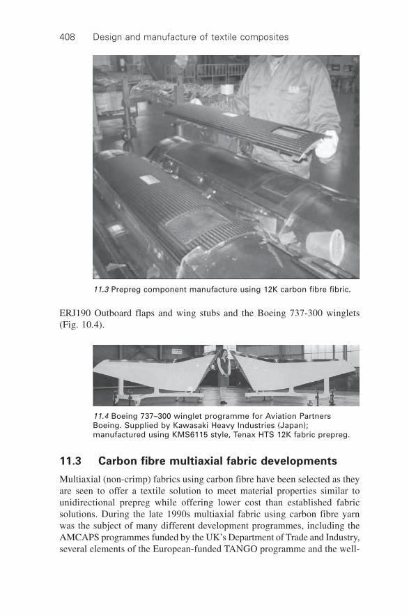
Design and manufacture of textile composites408
ERJ190 Outboard flaps and wing stubs and the Boeing 737-300 winglets(Fig. 10.4).
11.3 Prepreg component manufacture using 12K carbon fibre fibric.
11.4 Boeing 737–300 winglet programme for Aviation PartnersBoeing. Supplied by Kawasaki Heavy Industries (Japan);manufactured using KMS6115 style, Tenax HTS 12K fabric prepreg.
11.3 Carbon fibre multiaxial fabric developments
Multiaxial (non-crimp) fabrics using carbon fibre have been selected as theyare seen to offer a textile solution to meet material properties similar tounidirectional prepreg while offering lower cost than established fabricsolutions. During the late 1990s multiaxial fabric using carbon fibre yarnwas the subject of many different development programmes, including theAMCAPS programmes funded by the UK’s Department of Trade and Industry,several elements of the European-funded TANGO programme and the well-

Aerospace applications 409
documented NASA composite wing programme (started by the DouglasAircraft Company – now Boeing). These development programmes initiatedand drove the improvement of the textile quality of the carbon multiaxialfabrics.
Initially the multiaxial fabrics manufacturing looms (two types are usedwithin the industry, Liba and Karl Mayer-Malamo) were hydraulically driven,which caused the placement of the filaments to be inexact and the generalmovement of the laying-down heads to be clumsy and damaging to thebrittle carbon fibre yarn. As a result, the earliest fabrics manufactured usingthis technology tended to exhibit poorly placed filaments, gaps and unevenstitching (Fig. 11.5a). Driven by the quality concerns of the aerospace industry,Liba in particular improved its multiaxial looms to use electronic controlsand electrically driven motors. This has improved the accuracy of filamentplacement and has acted to reduce the damage of the carbon fibre yarn bycontrolling acceleration forces and using improved fibre handling mechanisms(Fig. 11.5b). This generation of machines, known as MAX3 Liba looms(Fig. 11.6), are the basis on which all present carbon fibre fabrics are producedfor aerospace application and development programmes.
11.3.1 Fabric development
Nearly all the developments of carbon fibre multiaxial fabrics have concentratedon the use of 12K carbon fibre yarn, owing to the cost implications of usinglower tow counts. During this time the major carbon suppliers have alsorealised that these developments require carbon fibre yarns that are suppliedas ribbon-like (flat) tows, able to spread and provide easy coverage once thetows are knitted through with polyester yarn to create the multiaxial fabric.For this reason, carbon fibre yarns such as Tenax HTS 5631 12K or TorayT700 12K carbon have been developed, which are supplied as a flat towwithout any false twists than can spread to provide gap-free fabrics.
Many problems still need to be overcome in the development of multiaxialfabrics. The mechanical properties of laminates produced using multiaxialtextile fabrics are still lower than equivalent unidirectional prepreg laminatesand the variation in properties is higher, dictating that the design propertiesare lowered. Limitation of low layer weights from multiaxial fabrics reducesdesign flexibility (due to large ply drop-offs) since at the present time individuallayer weights are limited to approximately 200 g/m2 (from conventional 12Kcarbon fibre yarn). The higher layer weights for thick constant sectioncomponents are attractive, since the issue of high fabric thickness and theability to apply triaxial or quadriaxial fabrics quickly is of great advantagewhen compared to unidirectional prepreg structures.

Design and manufacture of textile composites410
11.5 400 g/m2 biaxial fabrics (±45∞) Manufactured using (a) older and(b) the Liba multiaxial technology.
(a)
(b)

Aerospace applications 411
11.3.2 Stitching thread
An issue of great interest for the future is the development and improvementof stitching thread technology. The polyester stitching used as a processingaid in holding the fabric imparts an inbuilt flaw into the microstructure of thefabric. When the structure of the fabric is viewed closely, the carbon fibrefilaments bundled by the stitching thread can be seen. This fibre bundlingcreates uneven fibre distribution at a microscopic level and is believed to bethe cause of lower material properties in certain orientations. As such, thelarger the stitching fibre used, the greater the fibre disruption, bundling and‘fish eyes’ within the microstructure of the fabric.
11.6 Liba multiaxial MAX3 machinery.

Design and manufacture of textile composites412
Presently, the standard in the industry is to use a non-sized 80 dtex polyestermultifilament yarn. Improvements are constantly underway, and recenttechnology available from Teijin Polyester Filament (Japan) allows theapplication of an unsized 33 dtex multifilament polyester yarn. The firstfabrics being developed with these finer stitching yarns show promisingimprovements.
11.3.3 Quality control
One of the most problematic issues for multiaxial fabrics is quality control.Many of the manufacturers of multiaxial fabrics have been used to supplyingindustrial or marine industries, which have much lower-quality requirements.The aerospace industry has the requirement for the highest quality controland product release specifications. The raw material standard, prepreg materials,have tended to require mechanical property testing (e.g. interlaminar strengthand tensile strength) from specimens taken from random samples within aproduction run.
With multiaxial fabrics this type of quality control would be too difficultto organise, owing to the variety of processing routes and resins that may beused. As such, there are developments underway to implement quality detectionusing computer graphical detection methods. Images of randomly sampledfabric samples could be digitised, analysed and compared against an acceptedstandard (Fig. 11.7). In this manner it is hoped that by controlling the yarnorientation, coverage, stitching density, etc., the fabric can be released easilyfor aerospace fabrication without the need for costly mechanical testing.
11.3.4 Lighter-weight fabrics
One of the most restrictive issues with carbon fibre multiaxial fabrics is to beable to produce very light-weight layers (i.e. lower than 150 g/m2) usinglower-cost 12K or 24K filament tows. In order to be able to spread the largertows to create closed, gap-free unidirectional layers, Liba has modified themultiaxial loom (named MAX5) such that the yarns are spread and laid ontothe fibre bed. The spread tows are clamped (Fig. 11.8) and held in place witha newly devised system instead of the usual pins around which tows areusually wrapped.
This type of multiaxial loom can also to pre-spread tows of carbon filamentyarn. Using pre-spread tows manufactured either from 12K or 24K yarn,layer weights as low as 50 g/m2 can be achieved. Widely spread carbon fibretows are available from a variety of sources, most of these being in Japan. Assuch the Liba MAX5 is capable of manufacturing quasi-isotropic (quadriaxial)fabrics with areal weights as low as 200 g/m2 (0.2 mm ply thickness).

Aerospace applications 413
11.7 Digital graphical control of multiaxial fabrics. Digital imageshows excessively large ‘fish eyes’ created by high knitting yarntension.
11.8 MAX5 Liba multiaxial technology is able to clamp unidirectionaltapes in position before assembling the fabric.

Design and manufacture of textile composites414
Example 1: Multiaxial fabric components – using interleaved RFI
GKN Aerospace has started series manufacture of lower wing access panelsfor the Airbus A380 (Fig. 11.9) using a newly developed technology thatinvolves interleaving layers of fabric with resin film (M36 epoxy film suppliedby Hexcel Composites). The components use a 440 g/m2 biaxial carbon fibre(Tenax HTS 5631 12K) multiaxial fabric (±45∞) manufactured by Saint-Gobain (UK), stiffened by a honeycomb core. The manufacturing methodrequires no autoclave, merely vacuum and heat for the fabrication of thesecomponents. Also, owing to the viscosity of the resin film, no adhesive filmis required to bond the laminate to the honeycomb. Because of the lower costmaterials, reduction in lay-up times and the need for lower cost processingtools (i.e. no autoclave), the component manufacturing cost is estimated tobe 30% less than a conventional fabric prepreg manufacturing route.
11.9 Airbus A380 lower wing access panels manufactured by RFIusing biaxial (±45∞) multiaxial HTS 5631 12K fabric supplied by Saint-Gobain (UK).
Example 2: Multiaxial fabric components – RFI, using resin film blocks
The pressure bulkhead developed for the Airbus A380 has been devisedusing carbon fibre (Tenax HTA 5131 12K) biaxial (0/90∞) multiaxial fabricsmanufactured by Saertex GmbH and is fabricated using resin film infusionwith 977-2 resin film supplied by Cytec Engineered Materials (Fig. 11.10a).The bulkhead uses a fabric preform supplied by Saertex, which is assembledand stitched to form an assembly. This preform assembly is rolled onto acore unit, that is supplied to Airbus for component fabrication (Fig. 11.10b).The preform is rolled out onto a convex form that is pre-covered with theresin film. This assembly is vacuum bagged in the conventional manner andcured in an autoclave.

Aerospace applications 415
11.10 Rear pressure bulkhead or the Airbus A380. (a) Assembledmultiaxial dry fabric preform and (b) finished component.
(a)
(b)

Design and manufacture of textile composites416
11.4 Improvement in standard fabric technology for
non-prepreg processing applications
11.4.1 Unidirectional fabrics
Unidirectional (UD) fabrics are commonly used for adding stiffness in structuressuch as wing skins, spars or stiffeners (gliders, small general aircraft). UDfabrics also allow the lay-up of complex laminates in a similar fashion to UDprepreg tape structures. UD fabrics manufactured using Liba multiaxial loomstend to allow the filaments in the 0∞ direction to wander. Hence the resultingmechanical properties have been low in comparison with UD prepreg. OtherUD materials have also been evaluated, such as dry UD tape held togetherwith a fibre mesh backing, which is usually coated with an epoxy resin or athermoplastic binder. The main problems with these types of UD tapes is thatthey have very poor impregnation properties, especially through-thickness.
To solve these issues and to be able to offer a UD fabric structure thatexhibits repeatable quality, easy impregnation without excessive pressureand high mechanical properties, a new generation of fabrics has been developedusing 12K carbon fibre yarns. In particular, advanced UD weaves using glassor thermoplastic (polyester) fibres in the weft direction to hold the carbonfibre yarns in place can be used as tape laid like products in similar mannerto UD prepreg (Fig. 11.11). The scaffolding structure of the support yarnsallows for good permeability of the fabrics for vacuum infusion processes
11.11 ‘Advanced Unidirectional Weave’ (AUW) fabric supplied byCramer (Germany) using Tenax HTS 5631 12K carbon fibre yarn.Epoxy powder binder is applied onto the fabric surface.

Aerospace applications 417
and the fact that the carbon filaments are not crimped allows the fabrics toexhibit high mechanical properties.
Since these types of fabric are manufactured on a conventional weavingloom, issues such as quality control and repeatability are well understoodand accepted by the aerospace community. There are numerous developmentprogrammes presently underway to use the opportunities offered by thesenew types of materials.
11.4.2 Non-crimped biaxial fabrics
The type of non-crimp woven fabric described above is also available inbiaxial form. As such there are development programmes and projects underwayto qualify and use these materials in new component forms.
11.5 Braided materials
Braided carbon structures have been used for many years in aerospaceapplications. The best known applications are propeller blades (see Fig.11.12) by Dowty-UK and Ratier-Figac-F. In recent years, braided materialshave also been used in shear web stiffeners for applications such as landingflaps for the Bombadier-Shorts CRJ, in development programmes such asTANGO or for reinforcement of support struts for Airbus components
11.12 Over-braiding of a propeller fabric preform using Tenax HTA5131 12K carbon fibre yarn.

Design and manufacture of textile composites418
(manufactured by SARMA, Lyon). In the USA the company Fibre Innovationsmanufactures complete cruise missile casing preforms in a complex braidingprocedure.
Bombardier Aerospace has developed a process to manufacture outboardwing flaps for the Canadair regional jet (Fig. 11.13). The components replacemetal outboard wing flaps, and are manufactured in a single injection processusing HTA 5131 6K carbon fibre fabric in the skins, stiffened by braided±45∞ socks folded to create shear webs.
11.13 Outboard wing flaps manufactured by RTM using HexcelRTM6, Hexcel Injectex Fabric, braid from ‘A&P’ using Tenax HTA5131 6K carbon fibre.
11.6 Tailored fibre placement
Since 1995 there have been several well-documented development programmesto use textile embroidering technology to place carbon fibre tows, then stitchthe tows into position using fine polyester monofilaments to produce complexpreform structures (Fig. 11.14). The most successful of these developmentshas enabled the company Hightex (Germany) to offer complex preforms forspecialist applications. Hightex has used this technology to construct a complexpreform structure for Eurocopter. The first components to be selected arehoop-fuselage frames for the NH90 troop transport helicopter.
For these frames the preform is built up from a backing structure consistingof specially woven band fabrics onto which the tow is placed. The componentsare manufactured using the RTM process in a two-part matched metal tool.

Aerospace applications 419
Even though the preform manufacturing process is expensive, the raw materialcost is low and the waste material is estimated to be less than 5%. It isunderstood that the metal component that this composite piece replaced was30% heavier and was more expensive to manufacture.
11.7 Preforming
11.7.1 Textile assembly
The company FACC (Ried Austria) has used new material and preformingdevelopments from Cytec Engineered Materials, to develop a demonstrationcomposite replacement part for a highly stressed aluminium spoiler centrefitting on the Airbus A340-400 (Fig. 11.15). Owing to the complexity of thecomponent RTM was chosen. The high fibre volume content and the complexityof the preform meant that a low viscosity resin which could quickly andthoroughly impregnate the dry fibre preform was required.
However, for the high compression strengths necessary in this application,toughened epoxy resins containing high levels of thermoplastic additives arerequired. The thermoplastic additives increase the resin viscosity dramatically.This increased viscosity means that it is very difficult to permeate a preform
11.14 Tailored fibre placement (TFP) uses a single carbon fibre yarnwhich is stitched in place to create a complex preform. Severalplacement heads are able to run in parallel.

Design and manufacture of textile composites420
without high injection pressures and temperatures. The ‘Priform’ systemdeveloped by Cytec Engineered Materials is said to overcome this problemby adding the thermoplastic toughener into the preform in the form of fibres,rather than including them in the resin system. The resin, a development ofa widely used and aerospace-qualified toughened epoxy resin (977-2) isknown as 977-20 and is a single pot system including hardener and acceleratoragents.
The polymer toughening agent is spun into continuous fibres and is co-woven and added as a 3D stitching fibre into the fabric preform. Thethermoplastic fibres are said to dissolve into the resin during cure at temperaturesabove 100 ∞C. The preform uses a standard aerospace type 370 g/m2 HTA5131 6K carbon fibre fabric. The component is manufactured using a matchedmetal RTM mould. Injection temperatures are initially low to avoid thethermoplastic component dissolving too soon, which would create variationsin the thermoplastic contents throughout the moulding. This component,which is now due to be applied into full series production, weighs 30% lessthan the original metal component and has passed all required certificationtesting for aerospace application.
11.7.2 Preforming using heat-activated binder-coatedfabrics
Thermoforming is the most well-known and accepted preforming assemblymethod either with the use of heated vacuum forming (Fig. 11.16) or heatedpress forming. In either case powder binders are applied to the fabrics tobond the layers together to produce a rigid preform. These binders are usuallyepoxy or thermoplastic based, and are compatible with the basic resin systemsso that the binder does not adversely affect mechanical properties. Several
11.15 Spoiler centre fitting manufactured by RTM using a complexperform produced using Cytec Engineered Materials PriformTechnology. Moulding by Fischer Advanced Composite Components.

Aerospace applications 421
different binders are used, although each is coupled with its own resin systemfrom specialised resin manufacturers (e.g. RTM6 from Hexcel Composites).
11.7.3 Preform assembly using stitching yarns
In very large preform structures such as the A380 pressure bulkhead, in orderto be able to confection fabric textiles or to add extra localised reinforcementin certain highly loaded areas, specialised industrialised stitching/sewingmachines have been developed and are used for a variety of aerospacepreforming applications.
The choice of stitching thread materials are limited to a small selection offibre types:
∑ Low tex carbon fibre (67 tex or 200 tex) yarn has been used for a varietyof stitching applications. The major limitation with direct carbon fibretow use is that the fibre has little knot strength and as such tends tofilamentise when looped. Airbus is known to use direct carbon fibre towto add reinforced stitching to preform stringers manufactured using RTM.
∑ Carbon stitching thread was supplied to the market up to the late 1990s byToray, but is no longer available. However, new developments from thecarbon fibre manufacturers could introduce a new carbon fibre sewingyarn into the aerospace market.
∑ Assembled carbon thread (stretch-broken assembled filaments from 12K/24K yarn). Thin assembled yarns are available for suppliers such as Schappe(France) who supply carbon yarns as low as 50 tex which can be used forstitching.
∑ Aramid threads or yarns are easily processed and give excellent out of
11.16 Heated vacuum performing facility used to form textiles coatedwith heat activated adhesive binders.

Design and manufacture of textile composites422
axis strength. Drawbacks include problems with ultrasonic inspectionwhere the areas which have been stitched cannot be analysed since thesignal range is too high. The second and most important factor for the lackof acceptance of aramid yarn for localised structural reinforcement ismoisture absorption.
∑ Polyester yarn is used as an assembly aid. No strength is gained from thematerial. Saertex uses polyester yarn as a processing aid in the A380preform (Fig. 11.17).
11.17 Preform assembly using stitching technology. (a) Stitchingstation used to assemble several layers of multiaxial fabric (Saertex,Germany); (b) stitched assembly of multiaxial fabric stringers onto afabric skin.
(a)
(b)

Aerospace applications 423
11.8 Repair of fabric components
Repairing aerospace composite components has always been a hotly discussedtopic. Through the mid-1990s to 2003 a programme involving all the majorairframe manufacturers (Airbus, Boeing, Embraer, etc.) and many of thelarge aircraft users (British Airways, Air France, Fed Ex, United, American,etc.) devised design methodologies, repair techniques and qualification ofmaterial systems using a variety of repair methods. The system chosen wasa plain weave fabric using 3K plain weave HTA 5131 carbon fibre and a two-part epoxy resin system Epocast 52A/B supplied by Huntsman.
The repair material is a ‘wet lay-up’ repair system that can be applied toa prepared damaged area using two laminating techniques, either the ‘squeeze-out’ or ‘vertical-bleed’ methods. Both methods use prepared layers of ‘wet’resin impregnated patches to repair airframe structures, both for monolithicor sandwich laminates. The completed repairs are cured under vacuumconditions at 80 ∞C.
The repair system is now qualified to a universal specification and thecertified data are available to all interested parties. As such there is now amaterial and laminating system that can be used in Aircraft repair stationsworldwide. This fabric repair material can be applied to repair all epoxy-based aerospace components whether they are manufactured using prepregor other material processing technologies.

424
12.1 Introduction
The use of textile composites offers attractive possibilities for the constructionindustry. Some potential advantages are the reduction of weight of construction,the (mass) production of complex form components, possible overall costreductions thanks to industrialised off-site manufacturing processes, reductionin construction time, and production of multifunctional components. In addition,from an architectural point of view, textile composites offer variety ofappearances: translucency, colour, surface texture, finish quality, etc.
Textile composites have been used in construction since the 1960s, andthough they do not hold a prominent place compared with that of traditionalconstruction materials, their use is on the increase. It is possible to categorisetwo different groups of textile composites used in construction: fibre reinforcedpolymers (FRP) (most commonly glass reinforced polyester (GRP), but alsoglass, carbon or aramid reinforced epoxides) and membrane structures (mostcommonly poly(vinyl chloride) (PVC)-coated polyester fabric andpoly(tetrafluoro ethene) (PTFE)-coated (Teflon®) glass fabric but with othercombinations such as silicone-coated glass, PVC-, PTFE- or silicone-coatedaramid also being used).
12.2 Fibre reinforced polymers
The introduction and understanding of new materials in an industry sector isnot a simple procedure. This is particularly true for the construction industryowing to its large segmentation. Nonetheless, there have been a considerablenumber of studies on applications and design guidance for FRP in construction.Even such early studies as those by Hollaway [1, 2] and Leggatt [3] are stillvery relevant today; it is normally suggested that architects or civil engineersnot familiar with these materials should be aware of FRP composites havingspecific anisotropic properties, which means that existing design considerationsmay not be relevant. In addition, their mouldability and relatively low stiffness
12Applications of textile composites in the
construction industry
J C H I L T O N, University of Lincoln, UK andR V E L A S C O, University of Nottingham, UK

Applications of textile composites in the construction industry 425
imply the use of structural surfaces and multifunctional elements. On onehand, the anisotropic nature of FRP, and the particularities of the manufacturingprocesses by which individual elements are produced, seem (on account ofmarket constraints and building regulations) to call for levels of productdevelopment and industrialisation at which the non-standard buildingcomponent cannot compete. On the other hand, their mouldability and thenecessity (on account of relatively low stiffness) to adopt geometricalconfigurations of structural performance, confer a strong design characterthat makes it difficult for individual components to attain the flexibility thatmost traditional materials may offer.
Although these two main characteristics may appear contradictory fromthe traditional perspective of buildings as ‘one-off’ creations, there are plentyof opportunities for integration by adopting new approaches to the nature ofthe whole procurement process. One possibility would be to integrate adaptabledesign to production processes at early stages (e.g. mass customisation),thus avoiding the role of the architect as we know it. Perhaps these possibilitiesare the key to widespread use of FRP.
Even though FRP composites still do not hold a prominent position inbuilding, they have attracted the attention of architects and engineers formany years. There was an initial rise in their application in constructionduring the 1960s and 1970s, a period during which a considerable number ofbuildings using FRP appeared. The reasons for the later reduction in theiruse are various, including the oil crisis (which importantly increased theprice of resins), the low quality control exhibited by some manufacturers(which gave GRP a bad image) and the unsuccessful approach with which inearly times the construction industry in general managed standardisation andprefabrication processes. In addition, because of the low structural requirementsof the average component, textile FRP composites have only occupied amarginal place in the construction industry. The majority of FRP used havebeen chopped strand mat combined with glass reinforced polyester, usingwet lay-up processes for (typically) cladding purposes. However, followingadvances in material technologies and owing to the economic need forindustrialised production, new processes and applications have been foundfor composites in construction relying much more on the use of textiles asreinforcement, thus opening a completely new sphere for their use. Polymercomposites are now employed to fulfil significant structural tasks such asconcrete strengthening, concrete retrofitting and the production of entirelightweight structures such as pedestrian bridges.
Manufacturing processes such as pultrusion and pre-impregnation as wellas the use of carbon and aramid fibres have gained significant importance inconstruction during the last decade. This has been especially the case in thearea of infrastructure, where composites offer important advantages regardingdurability (corrosion resistance) and ease of installation (light weight). These

Design and manufacture of textile composites426
are crucial qualities at present, as a large proportion of the reinforced concreteinfrastructure in the developed world is reaching the end of its life span.Examples of the various bridge decking systems using pultrusion processesare ACCS (Advanced Composite Construction System) from MaunsellStructural Plastics, ASSET (Advanced Structural System for Tomorrow’sinfrastructure) developed by a European consortium including FiberlineComposites and Mouchel Parkman, and Duraspan® developed by MartinMarietta Composites. An example of the use of pre-impregnated processesfor strengthening and retrofitting is provided below as a case study. Anotherinteresting field is the use of 3D textiles; a good example is Parabeam®,which uses velvet weaving techniques with E-glass, to produce an integralsandwich panel.
At the moment, the construction industry represents an important fractionof the total tonnage of composites being consumed, 11% being the figure forthe UK [4] and 16.3% for the EU [5]. In both cases the construction industryrepresents the third major market for composites, but unlike other sectorswhere composites are used, in the construction industry plastics in generaldo not account for even 1% of the materials used [6]. Taking into account thesize of the construction industry and the various current advantages ofcomposites for building purposes, the above illustrates the enormous potentialfor a greater use of polymer composites in the construction industry.Accordingly, an increasing number of academic–industry projects and networks,such as Network Group for Composites in Construction (NGCC) and PolymerComposites as Construction Materials, on the use of composites in constructionare being developed in the UK and abroad. The future of FRP composites inconstruction looks very promising.
12.3 Membrane structures
Coated textile membranes form a class of flexible textile composites that areused for small- to medium-span enclosures (usually roofs and air-halls),where their properties of lightness, translucency, high tensile strength, durabilityand fire resistance may be exploited. Here the textile is the primary load-carrying component of the composite while the flexible coating protects thetextile from environmental degradation (e.g. the effects of UV light, moistureand pollutants) and creates a weather-tight enclosure.
Of the most commonly used yarn materials, polyester exhibits good tensilestrength, flexibility and significant elongation before yield, while glass fibreshows brittle behaviour and low elastic strain [7]. Thus polyester fabric-based membranes have greater tolerance to dimensional errors in manufacturing,as they may be stretched more easily to fit on site, and they may be used indeployable membrane structures. Conversely, glass fabric-based membranesrequire more accurate manufacture and can be more easily damaged whenfolded.

Applications of textile composites in the construction industry 427
The base fabric is generally woven in either basket or Panama weave,with the latter providing better mechanical properties [8]. One or more coatingsare then applied, the most common being PVC for polyester fabric (usuallywith a top coat of acrylic lacquer, weldable or non-weldable poly (vinylidenefluoride) (PVDF) lacquer, or poly (vinyl fluoride) (PVF) film [9]) and PTFEfor glass fabric (with, for example, a fluorinated ethylene propylene (FEP)topcoat to enhance impermeability, fungal resistance and weldability [10]).Other coatings are available, such as silicone, which is used primarily onglass fabric, giving a more flexible membrane than the more common PTFE-coated glass and offering greater translucency. Their perceived disadvantagehas been a tendency to attract dirt more readily than the ‘self-cleaning’ PTFEmaterial, although new surface treatments have overcome this, promptingrenewed interest in their application.
Unlike the majority of conventional building materials, textile membranesdisplay anisotropic, non-linear stress–strain behaviour, have negligibleresistance to bending and low shear resistance. The structures for which theyare used are geometrically non-linear under load. This requires a quite differentapproach to their design. To obtain some understanding of this difference,one might imagine the behaviour of a straight thread spanning between twosupports. This is unable to resist loads applied to it (except loads applied inthe direction of the thread) unless it deflects from its original straight profile1
(i.e. the geometry changes). The profile of the deflected thread will also varyaccording to the applied load configuration. Equally, a textile membranesurface cannot remain perfectly flat if it is to resist loads applied out of theplane of the surface and will change its form according to the loading.
Snow (or rainwater) and wind are the most common external appliedloadings in the case of textile membrane roofs. The former acts verticallydownwards under gravity while the latter acts perpendicular to the membranesurface and can be either pressure or suction, depending on the wind directionand orientation of the surface. Both types of load are of much higher magnitudethan the membrane self-weight, which is typically less than 1.6 kg/m2. Thusto better resist the applied loads, textile membrane structures usually havedouble curvature and to reduce deformation under applied load the surfacesare prestressed. The curvature is anticlastic (Fig. 12.1) in the case of membranestensioned externally (e.g. by masts, arches and edge cables) or synclastic, inthe case of inflated and air-supported membranes, which are pretensioned byinternal air pressure (Fig. 12.2). Hence, before carrying out an analysis to
1 In theory, for a straight horizontal thread to resist vertical load (even its own weight),without deflecting from the original straight profile, would require an infinite tension toexist in the thread. The thread actually hangs in the shape of a catenary under its self-weight.

Design and manufacture of textile composites428
determine the stresses in the surface, the engineer must first determine theform of the membrane for the specified support (boundary) conditions. Thisprocess is known as ‘form-finding’ and is carried out using specialised software.Only once the membrane form is established can the stresses in the surfaceand forces in supporting elements be assessed.
12.1 Simple anticlastic form of a small canopy, Millennium Garden,University of Nottingham, UK. The form has two high and two lowpoints creating a classic saddle surface (photo: John Chilton).
12.2 Synclastic form of the air-inflated membrane tubes for thedeployable roof of the Toyota Stadium, Toyota City, Japan (photo:John Chilton).

Applications of textile composites in the construction industry 429
A further peculiarity occurs because coated textile membrane material isproduced in rolls of a specific width and length, the precise dimensionsdepending on the manufacturer. Therefore, as in the tailoring of garments,the cloth must be patterned and cut in such a way that individual planarpieces, when assembled, approximate to a double-curved surface. In the caseof membrane roof structures this surface may be of considerable size. Thepattern is normally arranged so that the warp and weft directions of thefabric follow the principal stress trajectories. Because the material is anisotropicand is also to be prestressed, it is essential that the correct allowance or‘compensation’ is made in the cutting pattern for the stretch of the fabricunder tension. Biaxial tensile tests are usually carried out to determineappropriate compensation factors for the material. An appropriate allowancemust also be made for overlap at the seams. Therefore, all pieces are cutslightly smaller than established from the designed form and are then stretchedto the required shape and size during erection, known as ‘stressing-out’. Thisensures that the form of the structure, as erected, is as close as possible tothat originally designed and should avoid unsightly wrinkles. Owing to thetranslucency of the fabric, seam lines are a very prominent feature and thefinal pattern is often determined by both engineering and architecturalconsiderations.
Extensive details of membrane material manufacturers, fabricators, designersand researchers and a wide-ranging database of projects, engineers andarchitects are provided by TensiNet [11], the EU-funded network for tensilemembrane structures.
12.4 Case studies
12.4.1 Boots building, Nottingham (FRP strengthening)
The Boots Building in High Street, Nottingham (Engineer: Taylor Woodrow,Manufacturer: Advanced Composites Group; Fig. 12.3) is a historical building(Grade II listed) whose steel structure dating from 1921 had lost 30% of itssection due to corrosion. For its recent refurbishment, the structure had to beable to carry loads superior to those specified by the original design. Aparticularly important problem was the flexural strengthening of the curvedcorner beams, for which (in two cases) FRP composites were used.
The solution chosen was a glass and high-modulus carbon fibre–epoxylow-temperature curing pre-impregnated system, maintaining fibre orientationsat 0∞ and ±45∞ to the directionality of the beams. After installation (Fig.12.4), the beams were vacuum bagged (Fig. 12.5) and heated to achieve afibre volume fraction of 65%. The vacuum method also ensured a resin voidcontent below 4%. The advantages of the solution include short installationtime, no disruption to the refurbishment process, and minimal additional

Design and manufacture of textile composites430
12.3 Elevation view of the Boots Building, showing the curved cornersection (photo: Advanced Composites Group Ltd).
12.4 Placement of a carbon prepreg layer around the flanges andweb of a steel beam (photo: Advanced Composites Group Ltd).

Applications of textile composites in the construction industry 431
weight or volume to the structure (about 5 mm in thickness). The latterallowed the position of the terracotta cladding to be maintained, thus complyingwith requirements from heritage authorities.
12.4.2 Inland Revenue amenity building, Nottingham(membrane structure)
Opened in 1995, the Inland Revenue complex (Architect: Michael Hopkinsand Partners, Engineer: Ove Arup & Partners), in Nottingham, UK, has at itsheart an amenity building (Fig. 12.6) which includes an indoor sports hall,covered by a single-layer, PTFE-coated glass fabric membrane. This is boundedon two sides by two-storey bar/restaurant facilities and by fully glazed façadesto the north and south, partially shaded by the membrane. The sections ofmembrane are supported by lenticular windows suspended from four mainmasts and tensioned between the rigid edge frames of the windows andcables linking peripheral masts, (Figs 12.7 and 12.8).
12.5 Future developments
The built environment as an important part of and medium for culturalexpression is now facing challenges of complexity to a hitherto unparalleledlevel. Digital computer-aided design (CAD) technologies, which allow for
12.5 A vacuum bag used to apply pressure on the compositematerial (photo: Advanced Composites Group Ltd).

Design and manufacture of textile composites432
the development of 3D intricate configurations, along with the possibility oftheir direct linking to manufacturing processes (CAD/CAM), are now becomingstandard in various industries. The implications of vast information availability,fast project development speeds and new techniques as mentioned, are alreadyof importance to the way we think, and thus design and build. In this context,textile composites offer extensive opportunities due to high flexibility ofphysical configurations, and to the industrial nature of the processes involvedin their production. One could easily imagine mass-customisation processesbeing employed by using for instance membranes, pre-impregnated composites
12.6 Membrane roof at the Inland Revenue amenity building,Nottingham, UK (photo: John Chilton).
12.7 Stressing out the membrane at the Inland Revenue amenitybuilding, Nottingham (photo: Alistair Gardner).

Applications of textile composites in the construction industry 433
or any other structural textile being automatically cut and sewn to form 3Dstructures that would comply with specific requirements. The textilereinforcements per se may have been tailored using different densities,directionalities and fibre types, to suit the individual structural and visualrequirements for each part of the component they would form.
In the case of FRP composites particularly, there is a growing concern forthe environmental impact of their production and end of life. There is significantinterest in the development of biodegradable fibres and resins, very oftenbased on the utilisation of natural substances. Recyclability issues have focusedattention on the use of thermoplastic matrices in construction. However,taking a more realistic view of the immediate future, and understanding theissue of sustainability from a broader perspective, it is certain that present
12.8 Cable and edge details, Inland Revenue amenity building,Nottingham (photo: Alistair Gardner).

Design and manufacture of textile composites434
applications of FRP composites will continue to spread. Thanks to theirefficiency, ease of transportation and assembly, they still will have much tocontribute towards global economic growth and environmental welfare. Thenear future of construction is also likely to be marked by the emergence ofnew ways of using FRP composites, probably in combination with traditionalmaterials (e.g. masonry, concrete, timber, steel and glass) to form hybridstructures. Furthermore, following an initial period of technical investigationand validation, a more liberal and creative use of the materials can be expected,where aesthetic values take foremost importance. An example of this is theF100 street station (Fig. 12.9), a glass–FRP hybrid structure being developed
12.9 F100 street station (design and 3D image: Rodrigo Velasco).

Applications of textile composites in the construction industry 435
within the Architectural Construction Research Group (ACrg) at the Universityof Nottingham.
Tensile fabric membranes have, until recently, have been used primarilyfor canopies and/or temporary enclosures where environmental performanceis not a high priority. However, with the increased use of textile membranesfor permanent or semi-permanent enclosures, for example the Inland Revenueamenity building described above and the Millennium Dome in London,there is a move to improve, in particular, their thermal and acoustic properties.To achieve this, one normally needs to provide at least a two-layer systemwith or without an intermediate thermal and/or acoustic insulation layer.However, this tends to adversely affect the desirable property of translucency.Consequently, textile membranes are currently being developed with additionalcoatings designed to improve thermal performance, such as low-emissivity(low-e) coatings and surface treatments that selectively reflect certainwavelengths of solar radiation. Some of these materials are being used in theNew Bangkok Airport Terminal, currently under construction [12].
12.6 References
1. Hollaway L., (ed), The use of Plastics for Load Bearing and Infill Panels, ManningRapley, Croydon, 1974.
2. Hollaway L., Glass Reinforced Plastics in Construction: Engineering Aspects, SurreyUniversity Press, Guildford, 1978.
3. Leggatt A.J., GRP and Buildings, Butterworths, London, 1984.4. Sims G., Bishop G., UK Polymer Composites Sector: Foresight Study and Competitive
Analysis, NPL Materials Centre/NetComposites, 2001 (www.netcomposites.com)5. Starr T., Composites, A Profile of the Worldwide Reinforced Plastics Industry, Elsevier
Advanced Technology, Oxford, 1995.6. Dufton P. and Watson M., Materials in Use and Developments in Markets, Composites
and Plastics in Construction, BRE, Watford, 1999.7. Houtman R., ‘There is no material like membrane material’, in Designing Tensile
Architecture, eds Mollaert M. et al, Proceedings of TensiNet Symposium, Brussels,2003, p 182.
8. Ibid, p 183.9. http://www.architecturalfabrics.com (last accessed 28 December 2003).
10. http://www.4taconic.com Taconic Architectural Fabrics Division (last accessed 28December 2003).
11. http://www.tensinet.com TensiNet (last accessed 28 December 2003).12. Schuler M. and Holst S., ‘Innovative energy concepts for the New Bangkok Airport’,
in Designing Tensile Architecture, eds Mollaert M. et al, Proceedings of TensiNetSymposium, Brussels, 2003, pp 150–167.

436
13.1 Splinting material
Splinting materials for the repair of broken bones are not only the largestmedical market for textile reinforced composites, but the oldest. The use ofplaster of Paris was certainly known by the 10th century as a support forfractures and other bone injuries of limbs. Because of the brittle nature ofplaster of Paris, it is probable that it was reinforced with textile materialsfrom a very early stage. However, the modern plaster of Paris bandage, stillvery extensively used, was not patented until 1851 by Antonius Mathysen, aDutch military surgeon.
Many orthopaedic surgeons strongly believe that plaster gives a muchbetter moulding to the limbs than other products. Plaster of Paris casts(Fig. 13.1), however, tend to have a high failure rate and have to be reappliedor repaired. Patient comfort is as important as having a light-weight, strong
13Textile reinforced composites in medicine
J G E L L I S, Ellis Developments Limited, UK
13.1 Plaster of Paris cast.

Textile reinforced composites in medicine 437
cast; not only does plaster of Paris fail in this regard but is also sensitive towater, which means that the patient cannot conveniently shower, and bathingmay be almost impossible.
The requirement for a splinting material is a high degree of stiffnesscombined with conformability. This fabric reinforcement must be capable ofbeing moulded around the awkward contours of limbs. The fabric is requiredto be of open construction to allow impregnation with a large quantity ofplaster. These requirements can conveniently be met by a leno wovenconstruction where the warp yarns cross over one another, locking the weftinto place (Fig. 13.2). Such a fabric is also less inclined to fray when cut.
13.2 Woven construction of splinting material.
Similar characteristics can also be obtained with various warp knitted andsome weft knitted constructions. A number of fibres have been used inconjunction with plaster, particularly cotton, although modern bandages onthe market contain combinations of elastomeric yarn and polypropylene,polypropylene and polyester, or even glass. Glass has fallen into disfavourparticularly among casting technicians, mainly because of the glass containedin the dust produced during cast removal. Other casting materials also includepolyurethane-coated fibreglass and 100% polyester and polypropylenereinforcing fabrics.
In most modern casting products, the product is delivered to the plastertechnician as a packaged product that requires dipping in warm water. Thiswill then harden after wrapping around the limb of the patient within 3 or 4min (Fig. 13.3). A cast is formed that is sufficiently strong, even capable oftaking the patient’s walking weight, within 20 min. Not only is this externalsupport splinting system commercially valuable in its own right, but it hasled to the technique of ‘bandaging’ bridge support pillars with textile reinforcedmaterials when they are assessed as being too weak for anticipated loads.

Design and manufacture of textile composites438
13.2 Walking support frame
Walking support frames provide vertical support for patients who havedysfunctional lower limbs. They provide a rigid support to assist in bothstanding and walking. Conventionally, metallic frames have been used, butbecause of the comparatively low stiffness of metallic materials the weightof metal needed frequently inhibits use of the frame by the patient, whotypically suffers from cerebral palsy. The reduction in both weight and volumeof a carbon fibre reinforced orthosis has led to marked improvements in thecontinuity of walking as well as an obvious enhancement to the quality oflife of the user.
Because of the greater stiffness and hence rigidity of the frame and itsincreased strength, larger patients are able to use composite orthoses moreconveniently and continue to experience improved walking capability. Althoughcarbon-based materials have brittle failure characteristics, the mode of failureof such devices is of progressive collapse and is therefore inherently safe.The use of composites in smaller orthoses, such as knee braces, is limited,
13.3 Wetting the casting product.

Textile reinforced composites in medicine 439
because metallic knee braces are required to be available in only a limitedrange of sizes to reduce stock holdings. They are not customised to the samedegree and metal can readily be bent into shape to fit the patient. Such afacility is not normally available with thermoset resin-based materials.
13.3 Bone plates
In orthopaedic surgery, bone plates and screws are often used to treatfractures, particularly of the long bones. Most bone plates are made of stainlesssteel, cobalt chromium and titanium alloys (Fig. 13.4). However, the elasticmodulus of these metals is much higher than the elastic modulus of humanbone (110–220 GPa in comparison with 17–24 GPa for human bone). Becausethere is a stiffness mismatch, the normal healing process of the bone tends tomodify itself, changing the whole cycle of the formation of a callus aroundthe broken section, the conversion of the callus to bone (in the processknown as ossification) followed by the union of the broken bones. Therefore,development has moved on to consider the use of thermoplastic polymer-based composites and further to thermoplastic polymer composites for boneplate applications.
13.4 Metallic implants: hip prostheses (top and bottom) and boneplate and bone screw (middle).

Design and manufacture of textile composites440
Possible toxic effects (particularly from unreacted monomers) of allimplanted polymeric products is of major concern. This, combined with thefact that thermoset bone plates cannot easily be bent to shape in the operatingtheatre, makes composites of limited attraction. Combinations of carbon/polystyrene, carbon/poly propylene, carbon/nylon, carbon/poly-(methylmethacry late) and carbon/poly (etheretherketone) for bone applicationshave all been considered. Manufacture has been by the conventional fabricationmethods for thermoplastic textile composites, including film stacking (wherebylayers of matrix and reinforcing fabrics are hot pressed to melt them together),co-mingling (where mixed yarns of reinforcing and matrix fibres are madeinto fabrics), hot pressing and the use of powders of matrix materials inbetween stacks of reinforcing fabrics.
One of the difficulties with composite bone plates is the necessity toprovide screw holes within the plate to allow fixation to the bone. Drillingholes reduces the composite load-carrying capacity owing to the damagecaused to the reinforcing fibres by drilling. However, if the hole is formedduring the impregnation stage or earlier without significant damage to fibres,the loss of strength can be minimised. Computer aided design/manufacture(CAD/CAM) fibre placement technology, as is possible using conventionalembroidery machinery, has been suggested for these applications (Fig. 13.5).Biodegradable materials have also been examined, but there are ongoingconcerns particularly about the possible toxicity of degradation products asthe materials are absorbed into the body.
Carbon hip prostheses have also been developed, which, being of composite,provide the potential to have controlled stiffness and stress distribution inthe femur. This could result in significant property improvements overprostheses developed from conventional metal working methods, so thatpatterns of stress closer to those in the natural situation develop. This givesbetter regeneration of bone and reduces the potential for loosening. However,long-term success has yet to be proven, and such prostheses are not yet onfree sale to surgeons.
External fixation devices made from iron were developed from horseshoesin Russia, now known as the Ilizarov ring fixator for fractures. The materials
13.5 Prototype carbon embroidered bone plate.

Textile reinforced composites in medicine 441
used have been developed and carbon is used with the main advantage ofweight reduction and radio lucency (Fig. 13.6). They are not widely used,however, and many surgeons prefer to stay with steel devices, often ongrounds of cost.
13.6 Illzarov ring fixators.
13.4 General application
There is potential for textile reinforced composites to be used in very manygeneral applications within the medical industry, in common with manyother areas described elsewhere in this book. For example, fabric reinforcedprinted circuit boards have applications in all walks of life including medicalequipment. Specific applications include those requiring a low attenuationof radiation, in particular X-rays. With the increased use of minimally invasivesurgical techniques requiring monitoring by X-ray during surgical operation,thin, non-metallic operating tables are useful in helping to reduce the radiationdose that is received by the patient and scattered to those working in thetheatre. Carbon fibre operating tables have particular value in this area: theycan be thin, yet retain the necessary rigidity. When covered with foam and a

Design and manufacture of textile composites442
waterproof cover, a carbon fibre-based operating table will have all theperformance characteristics needed.
13.5 Living composites
A number of textile materials can be used to reinforced natural tissues, aswell as replace them. Textile surgical implants, such as suture threads, havebeen in use for many generations and over the past 40 years there has beenextensive use of polyester woven and knitted tubes in the replacement ofarteries. More recently, however, textile structures have been developed thatwill act as a scaffold for natural tissue re-growth, the textile remainingwithin the body for the rest of the patient’s life and forming a living textilereinforced composite. One example is the Leeds–Keio artificial ligament forthe replacement of the anterior cruciate ligament of the knee. The textilestructure of this device is a mock-leno weave (Fig. 13.7) formed into acomplex pocketed integrally woven tube (Fig. 13.8). During the operativeprocedure a bone plug is removed from a biomechanically appropriate siteon both the tibia and the femur before a bone tunnel is drilled through thecentre of the joint in the optimum position to join the two bone plug sites.The pocketed tubular woven fabric is threaded through the bone tunnel andthe bone plug inserted within the pocket at one end of the textile structure.The ligament device is pulled tight through the bone tunnels and the secondbone plug placed within a pocket formed at the other end of the artificialligament.
13.7 Mock leno woven tape.

Textile reinforced composites in medicine 443
Post-operatively, the bone will grow between the bone plug of both thefemur and the tibial bones to lock the textile structure in place. Along the restof the length of the polyester device natural tissue ingrowth will occur. Asthe knee is flexed and loaded, the tissue eventually orients itself and a naturalcomposite of ligamentous connective tissue reinforced by polyester fibre isformed in a true tissue/textile composite material.
13.8 The woven pocket tape used in the Leeds–Keio artificialligament.

444
14.1 Introduction
Conventional composite materials generally consist of a reinforcing textilestructure and a surrounding matrix with other mechanical properties. Bycombining two or more materials, the best properties of each material arecombined. The reinforcing fibres can supply strength and stiffness in anywanted direction, while the (generally polymer-based) matrix protects themostly brittle fibres against shocks and chemical agents. Whether or notmechanical stresses and strains are efficiently transmitted between fibres andmatrix depends on the adhesion between the both of them. Using (physico-)chemically compatible components is thus necessary when designing acomposite. Fibre/matrix compatibility is enhanced by applying sizings onthe fibres, thus avoiding delamination between fibres and matrix.
The use of textile composites in sports gear is relatively new. In the earlierdays, other materials were used. Calfee and Kelly1 report that natural materials(e.g. wood) were initially used because of their good shock absorption, butthese had many drawbacks. According to these authors – together with Jenkins2
and Axtell et al.3 – their anisotropic nature results in low perpendicularstrength, and their large variation in properties and high moisture absorptionresult in unwanted deformations.
In the 1970s light-weight metals such as aluminium and titanium becamepopular2. These provided higher stiffness and a significant reduction inweight1,2. However, since aluminium has no fatigue stress limit, even smallstresses contribute to fatigue1. Combined with its great flexibility, this led tooverbuilt designs1. Other drawbacks include its high shock transmittance(resulting in, e.g., tennis elbow) and inherent isotropic nature, which leavesno freedom to meet mechanical demands in different directions (as opposedto composites)1.
Later on, glass/epoxy composites, followed by carbon/epoxy and others,replaced metals2. These anisotropic materials allowed the ‘insertion’ of(mechanical) properties at certain places where extra strength is required1, 2.
14Textile composites in sports products
K V A N D E V E L D E , Ghent University, Belgium

Textile composites in sports products 445
Miracle and Donaldson4, Spry5 and Mattheij et al.6 mention that, by changingthe amount, direction and type of reinforcement, one may vary propertiesalong a certain cross-section, resulting in an optimal combination betweenperformance and low weight. According to Jenkins2, Spencer7 and Chouet al.8 composites provide higher specific stiffness, fatigue performance andshock damping than metals.
One of the latest developments is the combination of composites withother materials. Composite or metal baseball bats, for example, cause excessiveball speed (injuries), while a combination of wood with E-glass (or graphite)fibre reinforced composite results in an optimal combination of ball speedcontrol and shock absorbance3, 4. Other good examples are modern skis thatcombine composites with metal and natural (and other) materials. Dependingupon the desired properties, a combination of materials is made in such away that optimal properties are achieved. According to Murphy9, thecombination of composites with other materials (e.g. in metal–compositecombinations) can also be interesting given that when composites do fail,they generally fail spectacularly.
The usefulness of composites in sports gear depends upon the intendedend-use. Some applications require good shock (and thus energy) absorption,while others require a minimal energy loss in order to generate high speeds.Most of the time, a balance between several more or less contradictoryrequirements has to be sought. The eventual properties of the product dependupon the materials used, the design and the production technology. Theeffects of changes in these factors, as well as resulting property changes, arediscussed below, together with numerous examples.
14.2 Materials
14.2.1 Reinforcing fibres
Fibreglass is the most classical reinforcement. Its specific stiffness equalsthat of steel and it is more flexible and tougher than carbon4, 5. Its use insporting applications however, is – according to Spencer7 and Jacoby10 –limited because of its poor fatigue performance and high vibrationtransmittance.
Carbon is five times stiffer than glass, but lighter than aluminium5. Togetherwith its good fatigue resistance this results, for example, in light and strongbicycle frames4, 7. Carbon’s vibration transmittance might be a drawback insome applications10. Graphite is even stiffer than carbon but also more brittle4.Its shock resistance makes it ideal for skis, bicycle frames and tennis rackets.
The ‘sweet spot’ transmits minimal vibrations when hit, and exists inequipment such as tennis rackets. Miracle4 and Goode Snow Skis11 reportthat the use of graphite broadens this spot, resulting in more ‘forgiving

Design and manufacture of textile composites446
equipment’, ideal for inexperienced players and for avoiding injuries (suchas tennis elbow).
Kevlar is a poly-aromatic amide that provides light-weight tensile strengthand toughness, combined with good vibration damping and impact resistance4,
10. It is used in skis and also in many types of protective gear4. Boron is muchstronger than carbon. Compression properties are especially good4. Combiningcarbon (tensile stiffness) and boron (compressive stiffness) results in asynergistic effect, i.e. the overall stiffness is better than could be predictedbased on individual strengths1. Boron can, for example, be used as longitudinalreinforcement in golf clubs4. Celanese12 produces light-weight Vectran®liquid crystalline polymer (LCP) fibres that are as strong as boron fibres.Their stiffness, however, is comparable to that of glass fibres. Their impactand shock resistance are outstanding, which leads to many possible uses,such as in golf clubs, bicycle wheels and tennis rackets.
Shock damping and fatigue resistance can further be increased by usingpoly(ethylene) (PE) fibres. A possible example is a carbon/PE reinforcedbicycle4. Further weight reduction is also possible by using ultra-high modulusfibres. Such carbon and graphite fibres can be obtained by stripping off theouter fibre layer, leaving the stronger core1, 13. This list of possible fibres isby no means exhaustive.
14.2.2 Resins
Generally resins provide good vibration damping (far better than metal)1.Conventional thermoset resins (such as polyester and epoxy) are often combinedwith epoxy and rubber modifiers that lower vibration transmission2. Onemust, however, make sure that vibrations are not completely eliminated sincethe player needs ‘information’ from the impact in order to play a ball well.
Unsaturated polyesters are the most commonly used in the compositesindustry because of their good mechanical and chemical properties, incombination with their relative cheapness. They are mostly combined withconventional glass fibre reinforcement. Epoxies, on the other hand, are moreexpensive but provide better wetting out of the fibres. Their strength andcorrosion resistance is better than those of polyester resins, and they aremostly used in combination with high-performance reinforcements (carbon,graphite, etc.) or with high glass contents. Vinyl esters have properties thatlie between those of polyesters and epoxies. When considering sportinggoods, epoxy is generally used as a matrix material because cost is not amajor issue. Epoxy furthermore provides better adhesion and consequentlyhas better resistance to harsh conditions such as water or moisture in general.
Thermoplastic resins offer very high toughness and durability. Comparedwith thermoset resins they have a higher damage tolerance, are 100% tougher,and are 600% more resistant to cracks and invisible damage. This makes

Textile composites in sports products 447
them ideal for use in heavy-duty equipment such as (nylon/carbon) hockeysticks14.
The following example illustrates the importance of the matrix. Vibrationand shock transmission is higher in conventional carbon/epoxy tennis racketsthan in those with a polyurethane-modified epoxy matrix, and certainly thanin those with a thermoplastic polyamide-6 matrix. The latter absorbs moremoisture but this only further reduces vibrations8.
14.3 Design
14.3.1 General
In general, using different fibre angles (reinforcement shapes), different pliesor thicknesses, different (combinations of) materials, etc., may all contributeto the eventual resulting properties1. But special techniques that are notspecifically composite related, such as microbearings or overall shapemodifications, may be also used to obtain the same effect13.
14.3.2 Reinforcement shapes
Only a few examples of reinforcement shapes are discussed here. Braidedreinforcements combine multidirectional reinforcement with an automatedprocess, high uniformity, few seams and overlap, and good drapingcharacteristics3, 4. Reinforcement angle and thickness can be greatly varied,resulting in products such as baseball bats that can appropriately be reinforcednear the area of maximum stress, namely the handle3. Use of braids alsoreduces torsion – compared with unidirectional reinforcement – such as inski ‘torsion boxes’ (see further on) or prepreg carbon braids in tennisrackets4, 7.
Weaves have lower draping characteristics, and overlaps are often necessaryto enable smooth load transfer between different plies. They may, for example,be used (as 0/90∞ weaves stacked at ±45∞) in combination with unidirectionalreinforcement in order to produce tennis rackets with high shear strength andstiffness (torque reduction)2, 8.
The ‘tailored fibre placement’ (TFC) concept is worth mentioning. Fibrepreforms with stress-aligned fibre orientations can be made, based on theembroidery technique that is also used for decorating purposes. This techniqueis suitable for lightweight parts with a complicated stress course, such asbicycle frames and brake boosters6. Completely unidirectional reinforcementscan also be used. These result in excellent flexural and tensile stiffness andstrength, but very limited torsion resistance. Generally, several forms ofreinforcement are combined in order to obtain the desired combination offlexural, tensile and torsional properties.

Design and manufacture of textile composites448
14.3.3 Materials
It is important to choose a material according to the desired effect. Stiffermaterials such as glass, carbon, graphite and aramide are needed when one,for example, wants to achieve high speeds. If not, some of the energy thathas been put into the system may be lost in deformations. A good exampleis the outside of skates.
Less stiff materials, on the other hand, are needed when some or moredegree of deformation is wanted in order to absorb shocks. Good examplesinclude protection equipment, but also the inside of skates. The latter can,for example, be made from heat-mouldable foams mixed with carbon fibres.When the boots are preheated, one is expected to step in and the interior ofthe skate is consequently remoulded in order to fit perfectly to the feet10.
14.3.4 Material partition and positioning
Differences in reinforcement and resin placement enable a shift in the centreof gravity. The ends of kayaks, for example, may contain more (light) PEthan the rest of the boat, enabling the kayak to move more easily over thewaves. Other examples include ski poles, bats and golf clubs; where shiftingthe centre of gravity can provide more speed and better equilibrum4.Pole vaults are another possible example. They are made stiffer at the buttend using a mixture of carbon and fibreglass in order to obtain optimalproperties5.
Combination with other non-composite materials may consist of usingfoams or honeycomb structures in order to reduce weight and increase (flexural)strength, e.g. closed cell foam is used between two layers of fibreglass inboating, while polyurethane (PUR) honeycombs or foams are used in thecore of ski ‘torsion boxes’ (see Fig. 14.2 on page 4544, 5). Quaresimin et al.15
mention the use of epoxy foam in between layers of carbon/epoxy for theproduction of bicycle cranks. Using lighter foam hardly affects the specificproperties of the end-product.
Damping rubber or thermoplastics, on the other hand, may be used forvibration damping in tennis rackets. The ‘ISIS’ (impact shock isolation system)in tennis rackets, for example, consists of a separated graphite handle that isreconnected using graphite rods encased in PUR elastomer or thermoplastic(e.g. nylon) resin13.
Overall, design features may also be effective in reducing torque. Stiffeningboth sides of the throat area and cross-bar with titanium/graphite in tennisrackets, for example, instead of using braided reinforcements will also reducetorque13.

Textile composites in sports products 449
14.3.5 Some special features
Many features (not specifically related to composites) are possible, but onlya few examples are given here. The insertion of thousands of microbearingsin tennis rackets allows the racket to store energy as it swings backwards.This energy is released as the ball is hit, adding kinetic energy and thusspeed to the ball. The increase of ball speed is combined with a reduction inshocks and vibrations13. Inclusion of piezoelectric materials, for example inskiing, is a possible future application. Its principle is the conversion ofmechanical energy to electrical energy that is consequently dissipated, thusreducing vibrations2.
14.4 Production technology
14.4.1 Continuous processes
Continuous processes are only suitable for (quasi) continuous cross-sections.Pultrusion, for example, is a relatively cheap way of producing profiles witha high level of unidirectional reinforcement. It involves pulling a profilethrough a heated die where it cures. Multidirectional reinforcement (mats),however, may also be inserted to provide transverse strength. Possibleapplications are ski poles and parts of carbon/nylon bicycle wheels4, 7.Suominen16 and Spencer7 also mention combinations with other techniquessuch as (filament-, co- or pull) winding or roll wrap. The latter enables theproduction of hollow shapes by working around a round mandrel. Using thiscombination of techniques leads to a combination of flexural and torsionalresistance. Continuous processes result in low property variations and possibleexamples include golf clubs and fishing gear4, 5, 7. The latter can be producedas a combination of continuous carbon fibres that are spirally wound (torqueresistance and transverse strength), unidirectional longitudinal glass fibres(vibraton transmittance) and longitudinal carbon fibres (flexural strength)5.
14.4.2 Discontinuous processes
Discontinuous processes are generally slow and expensive, but they arenecessary when cross-sections vary. Most sporting goods have complex shapes,thus necessitating the use of discontinuous processes. Tennis rackets may bemade by resin transfer moulding or compression moulding (with internalbladder), while a special technique such as balloon moulding (that does notrequire rigid tools) may be suitable for baseball bats3, 7. Carbon/epoxy bicyclesand carbon/glass/aramid surf paddles are generally integrally moulded4, 17.Again, many other examples are possible: the number of possible techniquesis virtually unlimited.

Design and manufacture of textile composites450
14.5 Applications
Several examples are given here. As will be demonstrated, different applicationsrequire different combinations of materials, design features and productionprocesses.
14.5.1 Pole vault
In pole vaulting, the early use of bamboo poles and of the aluminium polesin the 1960s have long gone. These poles have been replaced with carbonfibre composites. Froes18 states that the ideal pole should be light and highlyflexible but also stiff and torsion-resistant, and that energy loss should beminimal. Nowadays, a typical pole consists of three reinforcement layers.The outer layer contains epoxy reinforced with unidirectional carbon fibres,which provide high stiffness for low weight and good fatigue resistance, andreturn a maximum of energy. The intermediate and inner layers respectivelyconsist of glass fibre webbing and wound glass filaments in an epoxy matrix,thus increasing the torsion resistance. The amount of glass and carbon can bevaried in such a way that the pole is much stiffer at the butt end5. Accordingto Bjerklie19, the pole may thus be custom built to the vaulter’s weight, take-off speed and hold technique.
14.5.2 Fishing gear
Fishing gear is somewhat similar in construction but requirements are different.Unidirectional carbon fibres provide flexural strength, while unidirectionalglass fibres provide the necessary vibration transmittance. Torque (torsion)resistance and transverse strength is obtained through continuous carbonfibres that are spirally wound5.
14.5.3 Bicycles
Bicycles have greatly evolved in the past few decades. The two major advancesare in the frame and wheels. Aiming at minimal frame bending combinedwith minimal weight, carbon fibre composites are the materials of choice ifthere is no concern over cost. A light-weight race bicycle (used by professionals)with a carbon reinforced frame, front fork and seat post is shown in Fig.14.1. In addition, frames have recently been produced from magnesium,aluminium, titanium and metal–matrix composites. Hybrid frames such ascarbon fibre reinforced composites combined with titanium have also beenproduced18. Carbon has a relatively high vibration transmittance but goodfatigue resistance, while the resin matrix has low vibration transmittance(good shock absorption), and titanium – as a metal – low fatigue resistance.

Textile composites in sports products 451
Combining these materials may result in combining high fatigue resistancewith increased shock absorption, while the overall weight remains low.
When going off-road, shock absorption becomes very important.Appropriately designed wheels can absorb a significant part of these shocks.Glass fibre reinforced nylon wheels have been produced to this end. Using athermoplastic matrix such as nylon (polyamide) results in better shockabsorption4, 18. Disc wheels (i.e. without the traditional spokes) made ofaluminium alloys and carbon fibre reinforced composites have been developedfor reasons of aerodynamics18. However, when crosswinds occur, these wheelsmake the bicycle difficult to control and so they become no longer beneficialin these conditions. A compromise might be a three- or five-spoke wheel,which besides making the bicycle more controllable, also cuts drag (byflattening the few remaining thin blades that slice through the air)19. Dependingupon the track and weather conditions, other materials and designs may benecessary in order to obtain the best results.
14.5.4 Golf
Golf clubs are nowadays lighter, longer and have a bigger head (with equalmass) than before. The net results are greater club head speeds – because ofthe long arc – and straighter shots (because of the bigger sweet spot). Theclub shaft may be constructed from graphite reinforced epoxy – and evenboron fibres may be used14 – while the oversized hollow head is made oftitanium9, 18. Changing material partitioning may also be helpful in shiftingthe centre of gravity, thus providing more speed4. These modern technologiesresult in an equalising effect (less gifted players perform much better owing
14.1 Lightweight race bicycle made of composite parts (courtesy:Giant, http://www.giant-bicycles.com)

Design and manufacture of textile composites452
to the reduced skill needed for playing golf), and change the game. This iswhy the US Golf Association has imposed a limit on the club head volume,as well as on the COR or ‘coefficient of restitution’. This is the ratio of thespeed of a ball before and after hitting the club and has been set at a maximumof 83%9.
14.5.5 Baseball/softball
Aluminium baseball bats have recently been banned in the major Americanleagues because they resulted in excessive ball speeds, which led to moreinjuries upon impact, but also because they altered the game itself as thefield became too small. However, after the ban in baseball, new double-walled aluminium and titanium softball bats were made. These provided abigger sweet spot, combined with a greater ball velocity18. These light-weight metal bats, however, acted as ‘equalisers’: they turned average hittersinto spectacular ones. Again, this type of bat was banned for security reasonsand now a limit is set to what is called the BPF or ‘bat performance factor’.For a conventional wooden bat, the BPF is set to 1.0. An aluminium bat thatreturns 10% more energy to the ball than the wooden one receives a BPF of1.1 and bats that exceed 1.2 BPF are considered illegal. Designers haveresponded to these restrictions by making new types of bats, e.g. hybridconstructions with carbon fibre reinforced composite and honeycombaluminium in a double-wall design9. The former provides strength and stiffnessbut is thought to reduce ball speed compared with aluminium, while thelatter provides a weight reduction combined with increased flexural stiffness.Speed control is also possible by adjusting the partitioning of materials (e.g.reinforcing fibres), thus affecting the position of the centre of gravity4. Thisis an example of how composites may also be used for security and fair playreasons, instead of only for conventional design reasons (speed, vibrationdamping, weight, etc.).
14.5.6 Tennis
Tennis rackets have evolved from wooden and metal frames (the latter wereintroduced in the late 1960s) to the modern ones, which are made of monolithicmetals, metal–matrix composites and carbon fibre reinforced composites.The goal in designing these modern rackets ranges from efficiency increase– i.e. accelerating the ball across the net – to damping the dangerous vibrationsthat can lead to tennis elbow. Accordingly, many types of rackets are possible.Increasing the rackets’ sweet spot, which depends upon the stiffness of theframe and the size and shape of the racket handle and head, can reducevibrations. Modern technologies have enabled the production of relativelylarge but still mechanically stable rackets, so the International Tennis Federation

Textile composites in sports products 453
has now imposed a limit on the size of the racket18. An example of such abanned racket is a type that used elongated strings in order to create a largersweet spot and generate more power and spin for less effort9.
The use of carbon fibre reinforced composite frames results in high stiffnessand corresponding efficiency. To reduce the high-frequency vibrations uponimpact, racket handles may be constructed by wrapping multiple fibre reinforcedlayers around a soft core of injected PUR or a honeycomb construction18. Analternative way of damping vibrations may consist of using a separatedgraphite handle and reconnecting it by using graphite rods encased in PURelastomer or a thermoplastic resin such as nylon13.
A state-of-the art racket may, for example, be based on a urethane core,graphite fibres and – to a lesser extent – Kevlar fibres. The graphite providesstrength and stiffness, and also prevents twisting of the racket head uponimpact outside the sweet spot. The Kevlar fibres lead to additional strengthand durability, and furthermore contribute to damping vibrations18. Usingweaves of these materials and stacking them at ±45∞ (or braidedreinforcement13), in combination with unidirectional reinforcement, resultsin rackets with high stiffness and high resistance to twisting2, 8. These state-of-the art rackets are lighter and stiffer, can be swung faster and give ballsmore rebound. Because of these high available speeds, modern tennis hasshifted in favour of the fast servers9. A possible solution might lie in imposingenergy-related limits as in golf and baseball.
Reduced torsion in tennis rackets may also be achieved by changing overalldesign features. Stiffening both sides of the throat area and cross-bar withtitanium/graphite, for example, may eliminate the need for using braidedfabrics in the frame. Other, not necessarily composite-related, design changesinclude the insertion of microbearings. These store energy, thus resulting inhigher ball speeds (efficiency) combined with shock reduction13.
Depending on the player level and his or her requirements a whole rangeof rackets is being made, using countless combinations of materials, materialshapes, design features, etc. This explains the great variations in racket types.
14.5.7 Kayaks
Competition kayaks were once made of mahogany veneers but are nowconstructed of a combination of carbon fibre cloth, Kevlar and epoxy resins.This stiff design minimises the amount of energy wasted in flexing as thehull passes through the water, thus making this energy available for upholdingthe maximum possible speed. Weight reduction is also remarkable, althoughcompetition kayaks are now subjected to minimum weight requirements.Because of this, other parts such as foot brakes and seat supports are nowbeing made of fibre reinforced composites in order to further reduce theoverall weight19. Again, changing material partition may also improve the

Design and manufacture of textile composites454
products’ qualities: by introducing more – light – PE in the ends than in therest of the hull, the kayak will more easily move over the waves4. Paddleswere once made of solid poplar but are now also made of composite materials.Changing the paddle shape into what is called a spoon-shaped ‘wing’ paddlehas further improved propulsion efficiency, although new paddling techniquesare required19. This is again an example of how new technologies can changea sport.
14.5.8 Skis and snowboards
Figure 14.2 gives an idea of the possible build up of a K2 ski20. In fact, thesame principle is also valid for water skis and snowboards. In the centre ofthe construction one can find the core. Aström21 and others report that thisflexible and lightweight part may be made of (PUR) foam, wood/foamcomposite or wood, or be simply empty4, 10, 22. Note the use of naturalmaterials. Sometimes channels are introduced into the core in order to furtherreduce weight and increase flexibility10, 23.
The core is wrapped with a composite material, resulting in the ‘torsionbox’. This torsion box is contoured to give the right amount of flex and
14.2 Possible ski constructions (courtesy: K2 Skis20).
Metal laminate construction
TNC construction
Torsion box construction
Modular structureGlassTitaniumGlassWood coreGlassTitaniumGlassBase material
Modular structureTitaniumTriaxial braidWood coreTitanium
Modular structureTriaxial braid
Wood core

Textile composites in sports products 455
spring and – especially – to eliminate twist24. This wrapping may consist ofglass/carbon/epoxy prepreg (reinforced in different angles) or triaxial braids,for example three layers of pre-impregnated fibreglass4, 10, 20, 22. The lattermay also be wet-rapped but this known to cause more mistakes. DesignNews magazine25 reports that wrappings consisting of co-extruded acrylonitrile-butadiene-styrene (ABS)/fibreglass sheet, rubber and fillers may also beused.
This central section is then sandwiched between a top and precision-milled base layer(s). Unreinforced thermoplastics are generally used as baselayer21. Moulding (and other) techniques are used for the construction ofboth layers. Multilayered skis may furthermore consist of sheets of glass/epoxy or reinforcing fibres such as carbon (strong, fatigue resistant), Kevlar(impact resistant), graphite (vibration resistant), titanium or others10, 21. Ontop of this construction, a secondary core is possible. This secondary core isbased upon modular technology and works both as a suspension system aswell as a mass damper20.
Different styles of snowboards depending upon the snow type are nowavailable. Deep, powdered snow requires more flexibe boards, while icierterrain requires stiffer boards. Because of their laminated construction, theboards in question require an epoxy adhesive that will keep the layers inplace through all types of terrain. This adhesive provides excellent wet-outof the fibreglass and other reinforcing layers, resulting in good fatigue andthermal resistance. Increasing the amount of epoxy without changing theamount of glass fibre results in stiffer boards, which perform better on icierterrain. The bindings can be made of nylon-based composites. Thisthermoplastic matrix provides good impact resistance, even in sub-zerotemperatures25.
14.5.9 Ice hockey
Ice hockey is an application where shock resistance is of major importance.Heavy-duty equipment such as hockey sticks can be made of nylon/carboncomposite. The thermoplastic matrix provides toughness, durability and shockresistance. Hockey skates may also be a combination of thermoplastic matricesand stiff fibres. The outside of these skates may be reinforced with stifffibres such as glass, carbon, graphite or Kevlar. The stiffer the fibres used,the less energy will be wasted on deformations10. A heel stabiliser wedgemade of an engineering thermoplastic elastomer, on the other hand, mayimprove the skater’s efficiency by allowing more forward flexing than traditionalskates while providing lateral and tendon support25. The inside of skates canbe made from heat-mouldable foams mixed with carbon fibres. The bootsare preheated and the user puts them on; the interior of the skate is consequentlyremoulded in order to fit the feet perfectly10.

Design and manufacture of textile composites456
14.6 Conclusion
Considering the given examples, one can easily see that a virtually limitlessnumber of material combinations are possible. Composite materials, but alsoother materials, are used for sports gear in order to obtain an optimalcombination of properties for each possible application. By furthermoreoptimising design and production techniques, one may obtain a product thatis suited for any possible combination of applications, conditions and playerexperience. Modern technologies also allow for the production of custom-built items.
In some sports these improvements have led to serious changes in thegame itself, the required skill to play the game, security issues, etc. As areaction to these technological changes, many sporting federations haveimposed limits on sporting goods. Inserting composite materials into sportinggoods has proved to be very useful – not only in improving overall performance– but also in controlling every possible property, thus leading to safer andfairer sporting. The future of composite materials in sporting goods probablyconsists of combining them with other materials, thus using the best propertiesof each constituent, and obtaining products that are suited for any givenrequirement.
14.7 Acknowledgement
The author would like to thank Stefaan Janssens for his contribution to thischapter.
14.8 References
1. Calfee C. and Kelly D., ‘Technical White Paper – Bicycle Frame Materials Comparisonwith a Focus on Carbon Fiber Construction Methods’, Calfeedesign, http://www.calfeedesign.com/calfee_TWP.pdf, 2002, 1–13.
2. Jenkins M.J., ‘Good vibrations – materials swing into action’, Materials World,2000 8(6) 11–13.
3. Axtell J.T., Smith L.V. and Shenoy M.M., ‘Effect of composite reinforcement on thedurability of wood baseball bats’, 32nd International SAMPE Technical Conference,Boston, SAMPE Publishing, 2000.
4. Miracle D.B. and Donaldson S.L., ASM Handbook – Volume 21 Composites, Ohio,ASM International, 2001.
5. Spry W.J., (1998), ‘Sports and Recreational Equipment’, in Dostal C.A., EngineeredMaterials Handbook – Volume 1: Composites, Ohio, ASM International, 845–847.
6. Mattheij P., Gliesche K. and Feltin D., ‘Tailored fiber placement – mechanicalproperties and application’, J. Reinf. Plast. Comp., 1998 17(9) 774–786.
7. Spencer B.E., (1998), ‘Composites in the sporting goods industry’, in Peters S. T.,Handbook of Composites, London, Chapman & Hall, 1044–1052.
8. Chou P.J.C., Ding D. and Chen W.-H., ‘Damping of moisute-absorbed compositerackes’, J. Reinf. Plast. Comp., 2000 19(11) 848–862.

Textile composites in sports products 457
9. Murphy M., ‘Blast off!’, Popular Science, 2002 (June issue, via http://www.popsci.com).
10. Jacoby M., ‘Olympic science’, CENEAR, 2002 80(5) 29–32.11. ‘Goode Snow Skis – Technology Overview’, http://www.goode.com/sstech.html,
2003.12. Celanese Acetate L.L.C., ‘Vectran – Grasp the World of Tomorrow, Engineering
Data’ http://www/vectran.net, 2003.13. Tennis Warehouse Recquet Technology Glossary, http://www.tennis-warehouse.com,
2003.14. ‘Falcon Sports Senior Hockey Sticks’, http://falconsports.com/Products/Senior.html,
2003.15. Quaresimin M., Meneghetti G. and Verardo F., ‘Design and optimisation an RTM
composite bicycle crank’, J. Reinf. Plast. Comp., 2001 20(2) 129–146.16. Suominen M., ‘High performance carbon fiber pultrusion profiles for the future’,
10th European Conference on Composite Materials, Brugge, 2002.17. ‘AT Paddles – Bentshaft Whitewater and Touring Paddles, AT2 series’, http://
www.atpaddle.com, 2003.18. Froes F.H., ‘Is the use of advanced materials in sports equipment unethical?’, J.
Minerals, Metals Materials Soc., 1997 49(2) 15–19.19. Bjerklie D., ‘High-Tech Olympians’, Technol. Rev., 1993 (January) 22–30.20. ‘K2 Skis’, http://www.k2skis.com/skis/technology.asp, 2002.21. Aström B.T., Manufacturing of Polymer Composites, London, Chapman & Hall,
1997.22. ‘Evolution Factory Tour’, http://www.evoski.com/factory_tour.html, 2002.23. ‘The Dynamic Ski Technology: Hyper Carbon, Texalium ...’, http://
www.skidynamic.com, 2003.24. ‘Surflight Hawaii Composite Controlled-Flex Technology’, http://www.surflight.com/
tech.html, 2003.25. ‘Plastics create a winter sports wonderland’, Design News, 1995 (20).

458
Anisotropic Having properties that vary with direction within a material.Autoclave A closed and heated pressure vessel used for consolidation
and curing of thermoset composites.Binder An agent (usually a thermoset or thermoplastic polymer)
used to provide cohesion to fibres, yarns or fabric layerswithin a preform.
Blend Mixture of two or more fibre types in a yarn.Braid; plait The product of braiding.Braiding; The process of interlacing three or more threads in suchplaiting a way that they cross one another in diagonal formation.
Flat, tubular or solid constructions may be formed in thisway.
Commingled A yarn comprising intimately mixed reinforcement andyarn matrix polymer fibres.Crimp The waviness or distortion of a yarn that is due to
interlacing in the fabric.Cure Change of thermoset resin state from liquid to solid by
the formation of crosslinks during polymerisation.Delamination Failure of a laminate by separation of layers, usually due
to external stresses.Denier A measure of linear density, corresponding to the mass
in grams of 9000 m of yarn.Dobby A mechanism for controlling the movement of the heald
shafts of a loom. It is required when the number of picksin a repeat of the pattern is beyond the capacity of camshedding (~8).
Drape The ability of a fabric to conform to a complex geometry.Ends Another name for warp yarns.Fibre Textile raw material generally characterised by flexibility,
fineness and high ratio of length to thickness.
Glossary

Glossary 459
Filament A fibre of indefinite length.Harness A frame positioned across a weaving loom with a set of
heddles mounted on it. This is used to raise or lower thewarp yarns.
Heddle A wire or thin plate with an eye through which a warpyarn passes.
Homogenisation Determination of material properties from unit cell orrepresentative volume analysis (RVE) for use in modelsat larger scales.
Intra-ply shear Deformation mechanism for bidirectional fabrics,involving in-plane shear of the material via rotation ofyarns at their crossovers.
Isotropic Having properties that do not vary with direction withina material.
Jacquard A shedding mechanism, attached to a loom, that givesindividual control of up to several hundred warp threadsand thus enables large figured designs to be produced.
Knitting A process to manufacture textiles via looping of yarnsaround a series of needles.
Laminate A composite material reinforced by a number of distincttextile layers (laminae, in this context).
Linear density The mass of a yarn per unit length.Locking angle The maximum level of intra-ply shear that can be achieved
for a fabric reinforcement before wrinkling/bucklingoccurs.
Matrix In this context, the polymer resin in which textile layersare embedded, providing the medium for load transfer.
Maypole braider A machine provided with three or more carriers that aredriven by means of horn gears along tracks that cross atintervals, enabling the yarn drawn from the carriers tointerlace to form a braid.
Monofilament A yarn consisting of one filament only.Net-shape Referring to a manufacturing process whereby the
component is produced in the correct dimensions andrequires no trimming.
NCF Non-crimp fabric; a fabric constructed from unidirectionalcrimp-free fibre layers, assembled together using a lightstitching yarn. More properly referred to as a warp knitwith inserted yarns.
Orthotropic Related to properties with three perpendicular axes ofsymmetry.
Permeability The property of a porous material (textile reinforcementhere) allowing pressure driven fluid flow.

Design and manufacture of textile composites460
Picks Another name for weft yarns.Plain weave The simplest fundamental weave pattern, where each warp
yarn interlaces with each weft yarn.Ply yarn Several strand yarns twisted together.Porosity The volumetric fraction of voids within a body (here
usually either a textile reinforcement or solid composite).Preform An arrangement of dry fibres in the three-dimensional
shape of the final component for liquid moulding processessuch as resin transfer moulding (RTM) and vacuuminfusion (VI).
Prepreg Pre-impregnated composites, comprising reinforcementscombined (usually) with a partially cured thermosettingpolymer.
RFI Resin film infusion; a manufacturing process that involvesconsolidation of interleaved layers of thermoset resin filmsand fabric layers.
Roving A flat yarn, normally sized, containing straight filamentsRTM Resin transfer moulding; a form of liquid moulding
whereby positive pressure is used to drive a liquidthermosetting resin into a mould cavity containing a dryfibre preform.
RVE Representative (or repeating) volume element; the smallestelement that can be used to describe the behaviour oftextile reinforcements or composites. In this context thisis normally equivalent to the smallest region that can beused to define the textile structure.
Satin A fundamental weave characterised by sparse positioningof interlaced yarns, which are arranged with a view toproducing a smooth fabric surface devoid of twill lines(diagonal configurations of crossovers).
Shed A gap between warp yarns where a weft yarn may beinserted.
Shuttle A weft insertion device, which is shut from side to sideof a weaving loom.
Sizing An agent, normally resin, added to yarn to keep fibres ina non-twisted yarn together and/or to improve adhesionto the matrix in composites.
Spinning A process, or series of processes, used in production ofyarns by insertion of twist.
SRIM Structural reaction injection moulding; a liquid mouldingprocess by impingement mixture of two or more reactivemonomers, which impregnate a dry fibre preform.

Glossary 461
Staple yarn A twisted yarn comprising fibres of predetermined shortlengths.
Tex A measure of linear density, corresponding to the massin grams per kilometre of yarn.
Textiles Originally woven fabrics, but now also applied to fibres,filaments and yarns, natural or synthetic, and most productsfor which they are the principal raw materials. Thisdefinition embraces, for example, threads, cords, ropesand braids; woven, knitted and non-woven fabrics; hosiery,knitwear and other garments made up from textile yarnsand fabrics; household textiles, textile furnishing andupholstery; carpets and other fibre-based floor coverings;industrial textiles, geotextiles and medical textiles.
Thermoplastic A polymer material that is softened by heating andhardened by cooling in a reversible process.
Thermoset A polymer material that is hardened by an irreversiblechemical reaction (curing).
Tow An essentially twist-free assemblage of a large numberof substantially parallel filaments.
Twill A fundamental weave with yarns interlaced in aprogrammed pattern and frequency to produce a patternof diagonal lines on the surface.
Twist Number of turns per unit length in a twisted yarn.Twisted yarn A yarn with fibres consolidated by twisting.Unit cell A representative unit of a textile or composite used in
analysis (usually equivalent to a representative volumeelement, RVE).
VI Vacuum infusion; a liquid moulding process where thepreform is enclosed between one solid tool and a vacuumbag, so that the driving resin pressure is one atmosphere.Also known as vacuum-assisted resin transfer moulding(VARTM).
Void A resin-free cavity within the composite (usuallycorresponding to entrapped air).
Volume fraction The volumetric proportion of a constituent in the composite(often an abbreviation for fibre volume fraction).
Warp The machine direction for a weaving machine/yarns inthe machine direction.
Weave The pattern of interlacing of warp and weft in a wovenfabric.
Weaving The action of producing fabric by the interlacing of warpand weft threads.

Design and manufacture of textile composites462
Weft (fill) The direction across the width of a weaving machine/yarns across the width of a fabric.
Wrinkle A defect formed during composite forming, formed viain-plane compression of the fabric/composite.
Yarn A product of substantial length and relatively small cross-section consisting of fibres and/or filaments with or withouttwist.
Yarn count The length of a yarn per unit mass.(number)Yield A measure related to yarn count or linear density,
corresponding to length per unit mass (yd/lb).

463
Index
ACCS (Advanced Composite ConstructionSystem) 426
acoustic properties 435active control 267, 268–73
case study 270–1, 272gate effectiveness 271–3SLIC 269–70
activity-based costing (ABC) 366–7actuators 269adaptive control 269additive flame retardants 342, 344Advanced Composites Group 183advanced unidirectional weave (AUW) fabric
416–17aerospace applications 182, 405–23
aircraft leading edge 324, 325braided materials 417–18carbon fibre multiaxial fabric developments
408–15non-prepreg applications 416–17preforming 419–22repair of fabric components 423standard prepreg processing 406–8tailored fibre placement 418–19see also Airbus family
air impingement ovens 227air looms 12Airbus family 396–401, 414–15
assessment on an aircraft section level401
fuselage panels 396–8manufacturing process performance 398–400material costs 398
alumina fibres 331, 335alumina trihydrate (ATH) 350–1aluminium 444
baseball bats 452amorphous polymers 205–6
amortisation of plant costs 371angle interlock 18, 20anionic polymerization of polyamides 216anisotropy 293, 458anticlastic curvature 427, 428antimony oxide 350, 351aqueous slurries 214aramid fibres 331, 334, 348, 349, 405aramid stitching yarns 421–2aromatic amine-cured resins 341–2assembled carbon thread 421assembly costs 380–2ASSET (Advanced Structural System for
Tomorrow’s infrastructure) 426asymmetric stress response 124autoclaves 182, 183, 185, 458
forming of thermoplastic composites 221autohesion 200automated fibre placement (AFP) 377, 398–400automated tape laying (ATL) 377, 398–9automation, level of 391, 392automotive body panels 195automotive transmission tunnel 153, 154, 155average pressure 93
balance of yarn crimp 25–7balloon moulding 449‘bandaging’ bridge support pillars 437baseball bats 445, 449, 452basket weaves 17bat performance factor (BPF) 452benchmark simulations 177bending
tow 113–15yarn 6–8
bending diagram 6–7bending moment 6–7bending rigidity 7–8

Index464
bias extension tests 63–4, 128, 129, 131–3normalization 134–7
biaxial continuum models 122–5biaxial in-plane tension see tensionbiaxial non-crimp fabrics 417biaxial tensile testing device 76–7bicycles 450–1binary data exchange 250–3binders 458
preforming using heat-activated binder-coatedfabrics 420–1
biodegradable materials 441bird-strike impact 324, 325bismaleimide resins 336, 344bladder inflation moulding (BIM) 223–4blank-holders 229–30blank-holding force (BHF) 171–2, 173, 174blank shape 172–5, 176, 177, 178blends 2, 458boat hull 220–1body panels, automotive 195bone plates 439–41Boots building, Nottingham 429–31boron fibres 331, 334, 446bottom (back) 13boundary conditions (BC) 245–7braid patterns 29–32braided fabrics 3, 27–34, 458
aerospace applications 417–18elastic behaviour 303–8internal geometry of 2D braids 32–3parameters and manufacturing of a 2D braided
fabric 27–32reinforcements for sports applications 4473D braided fabrics 33–4
braiding 27–9, 458braiding angle 32branch and bound search (BBS) 255–8, 259breather layer 184bridge support pillars, ‘bandaging’ 437Brinkmann equation 55buckling, fibre 116bulk melt impregnation 206
Cai-Gutowski compaction model 70–1, 104–5cam shedding mechanisms 13CAMSYS Automated Strain Analysis and
Measurement Environment(ASAME) 137–42, 143
carbon fibre 345aerospace applications of reinforced
composites 405–23CF/polyamide material 383–95properties 331, 333–4
sport applications 445–6stitching applications 421
carbon fibre composite plate (CFRP) 322–4carbon fibre operating tables 441carbon fibre-PEEK systems 214carbon hip prostheses 441carbon stitching thread 421carbon 2 ¥ 2 twill weave 78, 80, 88, 89Cartesian product 276cell models 54–5
see also unit cellcentre of gravity 448ceramic coatings 357–9channels 42–6char 343, 347–8, 353, 355–7char-bonding structures 352characteristic functions 22, 23–4, 52characterization methods 63–8, 129–37
bias extension test 63–4, 128, 129, 131–3normalization of test results 131, 133–7picture frame test 64–8, 69, 128, 129–31, 132,
161chemical properties
fibres 332–5matrix polymers 335–46
chopped (discontinuous) fibres 1, 333classical laminate theory (CLT) 301–2, 305–7coatings
flame-retardant 332, 357–9to improve acoustic and thermal properties
435co-compression moulding 233–5coefficient of restitution 452coefficients of compression 8–10combinatorial search (CS) 281–5commingled yarns 200, 458
consolidation of 201commingling 208–14compaction 62, 82–3, 85, 87–8, 88–107
behaviour 92–6effects of variable parameters 99–104importance in processing 88–92modelling 104–7of preform during mould closing 261and relaxation curves 96–9testing rig 95–6tow compaction 8–10, 96
compaction master curve 106–7compensation 429complex weaves 17compliance matrix 295compliant core 203, 233–5compressible yarns 25–7compression of yarns 6, 8–10

Index 465
compression mouldingco-compression moulding 233–5continuous 233, 234
computer-aided design (CAD) 431–2, 440computer-aided manufacturing (CAM) 432, 440consolidation of thermoplastic composites 198,
200–5effect of fabric deformation 202–3internal stresses and spring-back phenomena
204–5void content reduction 203–4
constant loading rate compaction test 99constitutive modelling 155–78
non-orthogonal model 125–6, 156, 157–62,177–8
application to forming simulation162–75
pre-impregnated composites 116–29constitutive models based on IFRM
122–5explicit models with fibre extensibility
125–6IFRM 116, 117–19predictive models based on
homogenisation methods 125shear force prediction based on energy
summation 126–9uniaxial composites 119–22
construction industry 424–35case studies 429–31, 432, 433fibre-reinforced polymers 424–6, 429–31,
433–5future developments 431–5membrane structures 426–9, 431, 432, 433,
435continuous compression moulding 233, 234continuous processes 449continuum mechanics 156, 158
biaxial continuum models 122–5IFRM 116, 117–19
control of resin flow 253, 254, 267–85active control 267, 268–73passive control 268, 274–85
controller (computer program) 269core, compliant 203, 233–5correspondence principle of viscoelasticity 117cost analysis 364–404
composites for the Airbus family 396–401cost build-up in textile composite applications
374–82assembly costs 380–2general input data 376manufacturing volume 376–8
materials perspective 374–6process machine cost 378–9process scrap 380tooling costs 379–80
cost estimation methodologies 366–74costs of prepregs 185, 186thermoplastic composite stamping 382–95
cost function (performance index) 254–5,256–7, 258, 259, 277
co-weaving 215cracks 42–6crepe weaves 17crimp 21–7, 77, 458
balancing 25–7braids 31, 32–3and elastic behaviour 305–7geometry of 21–5
crimp interval parameters 19–21critical fracture energy 320–1crossover shear 114, 115, 126–7crossover slip 114, 115crystallization shrinkage 203–4cure 243, 458curvature, radius of 6–7cycle time 391, 393Cyclics Corporation 226cyclics technology 217Cytec ‘Priform’ system 420
damage mechanics 315–16, 317–19Darcy’s law 189, 198–9, 245data acquisition hardware 268–9data exchange modes 250–3decision trees 269dedicated plant scenario 389, 390defects in the preform 260–1deformation mechanisms 111–16
effect on consolidation of thermoplastics202–3
see also under individual mechanismsdegassing 192degradation, matrix 228–9delamination 315, 323–4, 458
modelling 319–22denier 4, 458density functions 274–6detection table 266diamond braids 29diaphragm forming 221–3diffusion 204digital camera images 355–7digital graphical control 412, 413dimensions 5, 6

Index466
directionality 151constitutive modelling 159–60, 166, 167,
169–70, 171Dirichlet boundary condition (BC) 245–7disc wheels 451discontinuous fibres 1, 333discontinuous processes 449discrete-event simulation 372distributed parameter systems 271disturbances in mould filling process 259–68divinylmethane diisocyanate tooling resin 220dobby shedding mechanisms 13, 458double cantilever beam (DCB) test 321–2drapable thermoplastic composites 199–200drape 458drape modelling 202
iterative draping simulation 151–5kinematic models 149–51see also forming simulations
DrapeIt software package 153dry fabric 162–5Duraspan 426
E-glass (electrical resistance) fibres 331, 333edge/boundary profile 164elastic behaviour 292–312
analysis of practical textile-reinforcedcomposites 302–8, 309
finite element modelling 308–12micromechanics 297–9off-axis behaviour and laminates 300–2orthotropic solids 293–5testing methods 296unidirectional properties 296–9
elastica model 22, 23–4elastomeric tool forming 203, 230–1electrostatic coating 214elementary vent configurations (EVC) 281–2empirical compaction models 104, 105–7end notched flexure (ENF) test 321ends (warp yarns) 10, 458energy minimisation algorithm 152, 153, 154energy summation 126–9environmental impact 433–5epoxy resins 446
flame retardation 350, 352–7flammability of composite structures 347properties 336, 339–42snowboards 455
exhaustive search (ES) 255, 256, 259, 269, 283,284
explicit FE analysis 314–15extended-chain polyethylene (ECPE) 348, 349extension, intra-ply 111–12
extension ratio 140–2, 143external coatings 332, 357–9external fixation devices 441extra stress tensor 118, 119, 122–3
F100 street station 434–5fabric tightness 17, 65–7failure behaviour 312–27
impact simulations 322–7ply and delamination failure modelling
315–22solution strategies for FE failure analyses
313–15failure criteria 315–17feedback control 254, 267, 268–73fibre angle 164, 165, 166, 167, 168fibre buckling 116fibre bundling 411fibre distribution mode 47, 48, 53–5
using 53–5fibre extensibility
constitutive models for viscous textilecomposites with 125–6
inextensibility constraint 117–18, 125fibre-matrix interface 345–6fibre reinforced polymers (FRP) (construction
industry) 424–6, 429–31, 433–5fibre spinning 2fibre volume fraction 93–4, 100, 101, 102,
106–7fibres 1, 458
costs 374interaction of stitching with fibrous plies
42–6and flammability of composite structures 346,
347properties 330, 331, 332–5reinforcing fibres for sports textile composites
445–6filaments 1, 459fill time 260
minimum 258–9film stacking 206finite element (FE) analysis 53–4, 72, 105, 125,
155, 157biaxial in-plane tension 85–8, 89, 91elastic behaviour 304, 307–8, 309failure and impact behaviour 312–27
impact simulations 322–7ply and delamination failure modelling
315–22solution strategies 313–15
forming simulation of NCF preform 170–1modelling of textile composites 308–12

Index 467
stamping simulation for woven dry fabric162–3
unit cell under tension 85–8, 89, 91 fire resistance see flame retardants; flammabilityfishing gear 449, 450FIT (fibre-impregnated thermoplastic) process 214fixed costs 367–8, 371flame retardants 332, 338, 342, 343–4, 350–7
conventional 350–1inherent flame resistance 332, 349–50intumescents 351–7, 357–9paints or coatings 332, 357–9
flammability 330–63composite structures 346–9imparting flame retardancy to composites 332,
349–59properties of fibres 331, 332–5properties of matrix polymers 335–46
float 14flow, models of 55flow enhancement media, optimal placement of
286–7flow front 246, 247–8
racetracking strength and 264, 265flow mechanisms 200–1flow pattern 260
feasible target flow pattern in set point–basedactive control 287–8
flowable core 203, 233–5fluid saturation 100, 101–2fluidised bed processing 214foams 448Ford Thunderbird X-brace component 370,
382–95manufacturing process 370, 385–6material type 286–7plant utilization 387–90production sensitivity studies 390–5thermoplastic composite material systems
383–4weight saving assumptions 384–5, 386–7, 391,
392form-finding 427–8forming simulations 149–80
constitutive modelling approach 155–75, 176,177
future direction 175–8mapping approaches 149–55prepregs 137–42
secondary deformation mechanisms140–2, 143
shear deformation 138–40, 141, 142four-step 3D braiding 33–4fracture energy 320–2
frames, bicycle 450–1Fulcrum 216full line costs, amortisation of 371, 388functional integration 381, 382fundamental weaves 14–16fuselage panels 396–401
gate effectiveness 271–3gates, injection 245, 246, 249–50, 267
active control 267, 268–73gate location optimization 254–9
branch and bound search 255–8minimum fill time case study 258–9problem statement 254–5
multiple gate optimization 286generator paths 149–51, 152genetic algorithms 269geometric approach to textile modelling 49–50geometrically consistent yarn model for fabric
tensile biaxial behaviour 83–5, 86glass fabric aircraft leading edge 324, 325glass fibre 405, 445
cost analysis for thermoplastic compositesystems 383–95
membrane structures 426properties 330, 331, 333
glass plain weavebalanced 77–8, 79, 83, 85, 86, 88, 90unbalanced 79–81
global structure stiffness matrix 313–14golf clubs 451–2graphical user interface (GUI) 249graphite 445–6, 453
halogenated additive compounds 338Halpin-Tsai equations 298–9hand lay-up
dry fabrics 398–400prepregs 396–400
harness 10, 11, 13, 459Hashin’s composite cylinder assemblage (CCA)
model 299heat-activated binder-coated fabrics 420–1heat flux 346–7heat release rate (HRR) properties 352–3, 354heat treatment 197, 198heddles 10, 11, 459heel stabilizer wedge 455hercules braids 29herringbone weaves 17hierarchical structure model 1–2, 47–59
fibre distribution mode 47, 48, 53–5implementation 55–9yarn path mode 47–53, 54, 55

Index468
high-pressure thermoplastic processing 226–33hip prostheses 441homogeneous continuum models 156homogenisation methods 125, 156–7, 459Hooke’s law 294horn gears 29hot air ovens 227hybrid prepreg systems 184, 185, 187hydroforming 231–2hysteresis 7, 99
ice hockey 455ideal fibre reinforced model (IFRM) 111, 116,
117–19, 156constitutive models for viscous textile
composites based on 122–5modified to relax constraints 126
ideal forming analysis 172, 178Ilizarov ring fixator 441impact behaviour 312–27
impact simulations 322–7implicit FE analysis 313–14impregnation 198–201, 206–17
bulk melt impregnation 206commingling 208–14co-weaving and warp knitting 215in-situ polymerization 215–17powder impregnation 214–15solvent impregnation 208
in-plane shear see intra-ply shearin-situ polymerization 215–17incompressibility constraint 117–18, 125incompressible yarns 25, 26inert fillers 338inextensibility constraint 117–18, 125infrared heating 227, 228infrastructure 425–6inherent flame-resistance 332, 349–50initial fibre volume fraction 97, 100, 101, 102,
106–7Injectex 190injection-compression processing 226Inland Revenue amenity building, Nottingham
431, 432, 433, 435inlays 29, 30, 31, 33Intelligent RTM 269–70inter-dispersed fabrics 215interleaved RFI 414interlinked reinforcing layers 346internal stresses 204–5inter-ply rotation 112, 113inter-ply shear 202inter-ply slip 112, 113, 202intersection codes 19–21
inter-tow shear 114, 115inter-tow slip 114, 115intimate contact 200intimate mingling techniques 199, 200, 205–17intra-ply extension 111–12intra-ply shear 62, 63–73, 111, 112, 140, 202,
459characterization techniques 63–8, 69modelling 68–73
intra-ply slip 114, 115, 133intra-tow axial shear 115, 119intra-tow transverse shear 115, 119intumescents 351–7, 357–9investment 391, 392Iosipescu test 296ISIS (impact shock isolation system) 448isostrain assumptions 304–7isostress assumptions 304–7isothermal BIM (isoBIM) process 223–4isothermal processing 197isotropy 459iterative draping simulation 151–5, 175
Jacquard machines 13, 459
Kawabata compression tester 9Kawabata Evaluation System for Fabrics (KES-
F) 62Kawabata model 69–70, 82–3Kawasaki Heavy Industries 407–8kayaks 448, 453–4Kevlar 446, 453kinematic drape model (KDM) 138, 139–40,
142kinematic simulations 149–51, 175Kirchhoff-Love assumptions 302, 310knitted textiles
elastic behaviour of 303–8warp-knitted 3, 35, 36, 66, 68, 69weft-knitted 3
knitting 36, 459warp knitting 37–40, 215, 437weft knitting 437
L-mould 265–7Ladevèze model 319laminates 459
finite element modelling 310–11off-axis behaviour and 300–2testing methods 296
lapping diagram 38–40last-filled region maps 278–81LBASIC 248–9, 254lead-lag effect 192

Index 469
leading edge, aircraft 324, 325Leeds-Keio artificial ligament 442–3left (S-) twill 15Leicester notation 38leno woven fabrics 437Liba multiaxial looms 409, 410, 411, 412, 413lighter-weight fabrics 412–15limiting oxygen index (LOI) 331, 333, 336, 348linear density 2–4, 459liquid composite moulding (LCM) 242–91
active control 267, 268–73disturbances in mould filling process
259–68flow through porous media 244–7gate location optimization 254–9outlook 286–8passive control 268, 274–85processes 242–4
liquid injection moulding simulation (LIMS)247–54
features of 248–53gate location optimization 254–9interaction with 248–9interrogation of simulation at each time step
249procedures 249–50, 251process model in design, optimization and
control 253–4tracers 250virtual experimentation environment 250–3
liquid moulding 181, 187–96RFI see resin film infusionRTM see resin transfer mouldingSRIM 188, 193–4, 460VI see vacuum infusion
living composites 442–3local pressure 93locking angle 63, 65–7, 132, 459longitudinal modulus 297–8longitudinal viscosity 115, 119–22loom speed 11, 12loom up order diagram 13looms 10–13
Liba multiaxial looms 409, 410, 411, 412,413
loop geometry 40–2, 43low-pressure thermoplastic processing 218–26lower wing access panels 414
machine costs 368, 378–9, 386machine gauge 40macroscopic flow 244–5macroscopic scale 1, 63
deformation mechanisms 111–13
maleimide resins 336, 344mandrel 27, 28, 32manufacturing line 368–71, 385–6manufacturing volume 376–8mapping approaches 149–55, 175
iterative draping simulation 151–5, 175kinematic models 149–51, 175
mass customization 432–3mass loss curves 353, 355matched rigid moulds 232–3material costs 374–6, 391, 393, 398, 399, 400material scrap see scrapmaterial type, and costs 386–7MATLAB 250–3matrix coding of weaves 18–21matrix degradation 228–9matrix polymers 459
costs 374flammability of composites 346, 347properties 335–46see also resins
matrix viscosity 120–2mats
multidirectional reinforcement 449random 94–5, 243
maximum strain criterion 316maximum stress criterion 316maypole braider 27–9, 459mechanical analysis 62–109
biaxial in-plane tension 62, 73–88compaction 62, 88–107intra-ply shear 62, 63–73
mechanical approach to yarn path modelling50–2
mechanical propertiescomposites 292–329
elastic behaviour 292–312failure and impact behaviour 312–27
fibre distribution mode 53–4fibres 330, 331, 332–5matrix polymers 335–46yarns 5–10
medicine 436–43bone plates 438–41general applications 441living composites 442–3splinting materials 436–8walking support frames 438
membrane forces 229–30membrane and shell elements 156, 170–1membrane structures 424, 426–9, 435
Inland Revenue amenity building, Nottingham431, 432, 433, 435
mesh generators 53, 54

Index470
meso-cell approach 156, 170–1mesoscopic models 47–53mesoscopic scale 1, 63
deformation mechanisms 113–15fibre buckling 115
metal-composite combinations 445microbearings 449, 453micromechanics 297–9microscopic flow 244microscopic models 52–3
fibre distribution mode 47, 48, 53–5microscopic scale 1, 63
deformation mechanisms 115, 119Millennium Dome 435Millennium Garden, University of Nottingham
428minimum energy principle 47, 50minimum fill time 258–9mixed mode bending (MMB) test 321mixed model for crimp 24–5model-based control 269modelling
compaction 104–7in-plane shear 68–73tension 81–5see also forming simulations; resin flow
modified weaves 17modular assembly 381, 382monofilaments 2, 459mosaic approach 304motorsport 182mould filling see resin flowmove (step) 14multiaxial multiply non-crimp fabrics see non-
crimp fabricsmultilayer forming simulations 177–8multilayered weaves 18–21multiple gate optimization 286
Navier-Stokes equation 55nesting 56, 94, 261–2, 303
optimized nesting 394, 395net-shape 459net-shape stamped sheet over-injection moulding
235, 236Network Group for Composites in Construction
426Neumann boundary condition (BC) 245–6neural networks 269New Bangkok Airport Terminal 435Newton’s second law of motion 314nominal vent configuration 267non-continuum mechanics-based models 156
non-crimp fabrics (NCFs) 3, 35–46, 459carbon fibre developments 408–15elastic behaviour 303forming simulation of NCF preform 168–75in-plane shear modelling 72, 73internal geometry 40–6iterative draping simulation 151–3, 154, 155manufacturing 36–40terminology and classification 35–6woven 416–17
non-deformable normals 302non-homogeneous continuum models 156non-isothermal BIM (non-isoBIM) process
223–4non-isothermal processing 197non-linearity 74, 75non-orthogonal constitutive models 125–6, 156,
157–62, 177–8application to forming simulation 162–75
NCF preform 168–75stamping simulation for woven dry fabric
162–5stamping simulation for woven
thermoplastic prepreg 165–8fibre directional properties 159–60shear properties 160–2
non-scission reactions 340non-uniform consolidation 202–3normalization 131, 133–7novolac resins 342number of cycles 100, 102–3number of layers 100–1NYRIM 192–3
object oriented programming (OOP) 55–6, 57–9off-axis behaviour 300–21.5 layered satin 18, 20open mould (wet lay-up) 181, 185, 186open preform structure 35, 36operator level 391, 395optical microscopy 355–7optimization 178
resin flow 253, 254, 276–85orthogonal multilayered weaves 18, 20orthoses 438orthotropy 157–8, 459
orthotropic solids 293–5ossification 439out-life 182outboard wing flaps 418outer protective surfaces 332, 357–9oven heating 220over-injection moulding 235–6

Index 471
paddles 454paper-point diagrams 13, 14Parabeam 426parallel-series (PS) model 306–7partial exhaustive search (partial ES) 283partitioning of sets 257–8parts count reduction 380–1, 382passive control 268, 274–85
case study 282–5combinatorial search 281–5last-filled region and vent fitness maps
278–81optimization problem 276–7
peak heat release rates (PHRR) 348, 349, 352–3,354
Peirce type models 22, 24percentage line utilization 371, 388–90performance index (cost function) 254–5,
256–7, 258, 259, 277permeability 189, 190, 245, 260, 459
racetracking 263–4permeability prediction modelling 53, 55phenol 338, 341phenolic resins 336, 342–4, 347, 350phenomenological compaction models 104–5physical properties
fibres 330, 331, 332–5matrix polymers 335–46
picks (weft yarns) 10, 460picture frame test 64–8, 69, 128, 129–31, 132,
161normalization 134–7
piezoelectricity 449pillar warp-knit fabrics 66, 68, 69plain weave 15, 460
balancing yarn crimp 25–7stamping simulation for woven dry fabric
162–5plait/stitch/pick 32plaiting see braidingplant utilization 387–90plaster of Paris 436–7plastic yield behaviour 124plied matrix technique 215plies 1, 313
interaction of stitching with fibrous plies42–6
ply failure models 315–19damage mechanics 317–19
ply yarns 2, 460Poisson’s ratios 294, 298, 299, 307pole vaults 448, 450polyamides (PA) 383–95
anionic polymerization 216
SRIM 193–4polybutylene terephthalate (PBT) 217, 226polycarbonate (PC) 217polyester membrane structures 426polyester resins 336–8, 446
intumescents 352–5polyester yarn 422polyether ether ketone (PEEK) 214polyetherimide (PEI) 208polyethylene (PE) fibres 331, 335, 446polyethylene terephthalate (PET) 383–95polyimide resins 344Polymer Composites as Construction Materials
426polymerization, in–situ 215–17polyphenylene terephthalate (PPT) 334polypropylene (PP) 198, 204, 383–95polytetrafluoroethylene (PTFE) 427polyurethanes 216polyvinyl chloride (PVC) 427polyvinyl fluoride 427porosity 203, 460porous media, flow through 244–7powder impregnation 214–15power law behaviour 123–4predictive simulation models 92
forming simulations see forming simulationspre-impregnated textile composites 125resin flow see resin flow
preforms 94–5, 460aerospace applications 419–22LCM
compaction during mould closing 261defects in preforms 260–1racetracking strengths 264, 265
preheating techniques 227–9pre-impregnated composites (prepregs) 110–48,
333, 339, 460aerospace applications 406–8characterization methods 129–37constitutive modelling 116–29construction applications 425–6deformation mechanisms 111–16forming evaluation methods 137–42, 143manufacturing with thermosets 181–7
advantages 183cost equation 185hybrid systems 185–6material systems 182–3processing 183–5
press-based processes 226–33pressure 92–3
thermoplastics 197, 198high-pressure processing 226–33

Index472
low-pressure processing 218–26see also compaction
pressure bulkhead 414–15pressure decay 100, 101pre-tensioning rig 65probability density functions 274–6process-flow simulation (PFS) tool 366, 371–4
input and operation 372–3output 374
process simulation models 106, 253–4process windows 217–18, 228–9production sensitivity studies 390–5productivity
of a braider 32of a loom 11
projectile (shuttleless) looms 12propeller blades 417pultrusion 215–16, 425–6, 449
quality control 412, 413quasi-static compaction 101–2
racetracking 262–8experimental measurement 265–7, 268modelling a racetracking channel 263–5successful mould filling despite 267–8see also active control; passive control
racetracking forecast 275–6use of manufacturing data for 287
racetracking sets 265–6, 275–6racing yachts 182random mats 94–5, 243rapid stamping technique 232–3rapier looms 12rate of deformation tensor 117, 118raw material costs 374–6, 391, 393, 398, 399,
400reachable set 287–8reaction injection moulding (RIM) 215–17reactive flame retardants 342, 343–4reactive impregnation process 384reactive thermoplastic (RTM) 225–6rectangular mould with triangular insert 270–1,
272rectilinear stamped sheet 235, 236recycling 391, 394–5reed 10, 11regular (plain) braids 29reinforced concrete 426reinforcement shapes 447Reissner-Mindlin assumption 311reject rate 391, 393relaxation 96–9, 100–2, 106repair of aerospace components 423
repeat 51braid 32weave patterns 14
repeated compaction cycles 102–4representative (or repeating) volume element 304,
4603D FE modelling of 307–8, 309see also unit cell
resin film infusion (RFI) 188, 194–6, 460interleaved 414using resin film blocks 414, 415
resin flow 242–91active control 267, 268–73disturbance in mould filling process 259–68flow through porous media 244–7gate location optimization 254–9liquid composite moulding processes 242–4LIMS 247–54outlook 286–8passive control 268, 274–85
resin infusion process (RIP) 242resin percolation 200resin transfer moulding (RTM) 181, 185, 188,
189–90, 242–3, 267, 460aerospace applications 419–20compaction 90, 92, 97, 98, 101–2, 103compared with SRIM 193in-situ polymerization 215–17reactive thermoplastic RTM 225–6
resins 335–46fibre-matrix interface 345–6flammability of composites 346, 347properties 336–45sports products 446–7see also matrix polymers
resistance to needle penetration 18, 19resoles 342rib weaves 17right (Z-) twill 15rigid/semi-flexible thermoplastic composites
199–200roll wrap 449rotation, inter-ply 112, 113rovings 2, 5, 6, 460rubber block pressing 231rule of mixtures 297–8
S-glass (high strength) fibres 331, 333Saint-Gobain Vetrotex process 213sampling time 269satin weaves 16, 460saturation 100, 101–2scaffolding effect 350scenario-based control 269–71

Index 473
scenario space 266, 276, 278mould symmetry and 285
Schappe commingling process 213–14scission reactions 336–7, 340–1scrap 380
recycling 391, 394–5screw holes 440Seeman composites resin infusion moulding
process (SCRIMP) 242–3selvedge 11semi-crystalline polymers 205–6semi-flexible/rigid thermoplastic composites
199–200semi-pregs 194, 195sensitivity studies 390–5sensors 268–9series-parallel (SP) model 306set point–based control 269
feasible target flow pattern selection 287–8shared memory blocks 250–3shear
crossover 114, 115, 126–7elastic behaviour of laminates 302, 310–11inter-ply 202inter-tow 114, 115intra-ply see intra–ply shearintra-tow axial 115, 119intra-tow transverse 115, 119non-orthogonal constitutive model 160–2,
165–6, 169–70, 171picture frame test see picture frame testshear force prediction based on energy
summation 126–9tow shear 113
shear angle 65energy summation 126–9forming evaluation methods 138–40, 141, 142non-orthogonal constitutive model 172, 174,
175, 177picture frame tests 130–1, 132
shear compliance curves 67–8, 69shear energy 152shear locking 311shear resistance 69–72shed 10, 11, 460shedding mechanisms 13shell elements 156, 170–1
thick 310–11thin 310
ships 358–9shock absorption 451short (discontinous) fibres 1, 333shuttle 12, 460shuttleless looms 12
silicone 427simulation-based liquid injection control (SLIC)
269–71, 272single diaphragm forming 222sinking of stitching 42, 46sizing 2, 345, 460skates 448, 455skis 445, 454–5slip
crossover 114, 115inter-ply 112, 113, 202inter-tow 114, 115intra-ply 114, 115, 133
smoke production 355smoothed particle hydrodynamics 324snow 427snowboards 455softball bats 452solvent impregnation 208SP Systems 183, 184spinning 2, 460splinting materials 436–8split-film knits 215spoiler centre 419–20sports products 444–57
applications 450–5design 447–9materials 445–7production technology 449
spring-back phenomena 204–5SPRINT process 184, 185, 187squeeze flow (transverse fibre flow) 200stamped preforms 235–6stamping 226–33
blank-holders and membrane forces 229–30compaction and 90–2, 97–8continuous compression moulding 233, 234cost analysis of Ford Thunderbird X-brace
component 382–95elastomeric tool forming 230–1hydroforming 231–2preheating technology for 227–9rapid stamp-forming with matched rigid
moulds 232–3stamping simulations
woven dry fabric 162–5woven thermoplastic prepreg 165–8
staple (short fibres) 1, 333staple yarn 461stiffening index 100, 102, 106–7stiffness 53, 295
classical laminate theory 305–7compaction and relaxation 97, 100, 102off-axis behaviour and laminates 300–1

Index474
sports application materials 448stitched composite ‘T’ joint 324–7stitching
forming simulation 151–5, 169interaction with fibrous plies 42–6stitching thread and carbon fibre multiaxial
fibre development 411–12stitching yarns 421–2strength factor 18, 19stressing-out 429structural elements 48, 51–2structural net 159structural reaction injection moulding (SRIM)
188, 193–4, 460structure 1–2, 3
textile structure models 47–59styrene 336sub-cells 304, 307sweet spot 445–6, 452–3symmetry, mould 285synclastic curvature 427, 428
‘T’ joint 324–7tailored fibre placement (TFP) 418–19, 447technical cost modelling (TCM) 366–71, 381
cost model output 371fixed and variable costs 367–8input data and assumptions 368model structure 368–71process-flow simulation tool 371–4
Technofire ceramic webs 359Ten Cate CETEX range 208tennis rackets 448, 449, 452–3tensile behaviour surfaces 75–6, 78–81, 86TensiNet 429tension 62, 73–88
analytical models 81–5, 86experimental analysis of biaxial tensile
behaviour 76–81tensile behaviour surfaces 75–6, 78–81, 863D finite element analysis of unit cell under
tension 85–8, 89, 91tension strain curves 78–81, 83tension tensor 75–6tex 4, 461text (command) data exchange 250, 252, 253textile structure models 47–59
fibre distribution mode 47, 48, 53–5implementation of textile hierarchical model
55–9yarn path mode 47–53, 54, 55
textiles 461thermal barriers 357–9thermal properties 435
thermal thickness 346–7thermal thinness 346–7thermoplastic composites 153, 193–4, 197–241
composite material forms 205–17consolidation 198–205costs 375high-pressure processing 226–33low-pressure processing 218–26mechanical properties 206, 209–12novel manufacturing routes 233–6process windows 217–18processing routes 217–33stamping see stamping
thermoplastic resins 205–6, 207, 208, 335–6,344–5, 446–7
thermoplastic RTM (TP–RTM) 225–6thermoplastics 461thermoset composites 181–96, 375
costs 375liquid moulding 187–96pre-impregnated 181–7
thermoset resins 335, 336–44, 446thermosets 461thick laminates 310–11thick shell elements 310–11thickness 93–4
laminate 192, 310–11see also fibre volume fraction
thin laminates 310thin shell elements 3103D braided fabrics 33–43D finite element (FE) analysis 72
elastic behaviour 304, 307–8, 309unit cell under tension 85–8, 89, 91
3D orthotropic elements 311–123D textiles 426through-thickness angle interlock 18, 20through-thickness compaction see compactiontightness
fabric 17, 65–7of a 2D weave 17–18, 19
tissue re-growth scaffolds 442–3titanium 444tolerances 280tooling costs 379–80, 391, 395top (face) 13torque 448
for yarn crossover 70–1torsion box 454–5tow 2, 461tow bending 113–15tow compaction 8–10, 96tow count 406, 407, 409tow shear 113

Index 475
tow squeezing 113–15tow twisting 113–15Toyota Stadium, Toyota City, Japan 428tracers 250traction error 269transverse viscosity 115, 119–22trellis deformation see intra-ply sheartriaxial braids 29, 30, 31, 33tricot stitched NCFs 72, 73tricot warp-knit fabrics 66, 68, 69truss and shell elements 156, 170–1Tsai-Wu quadratic failure criterion 316–1712K carbon fibre fabric 407–8, 409twill weaves 15–16, 461
carbon 2 ¥ 2 twill weave 78, 80, 88, 89twist 4, 461twist angle 4–5twisted yarns 2, 461twisting, tow 113–152D braided fabrics 27–33
internal geometry 32–3parameters and manufacturing 27–32
2.5D carbon fabric 88, 91two-step 3D braiding 33–4
ultra-high modulus fibres 446ultra-high molecular weight polyethylene
(UHMWPE) 331, 335unbalanced glass plain weave 78–81unevenness (coefficient of variation of linear
density) 4uniaxial CFRC 110
constitutive behaviour 119–22, 124unidirectional (UD) fabrics 416–17unidirectional properties 296–9
prediction 297–9testing methods 296
unit cell 31, 32, 159, 304, 461cell models 54–53D FE modelling of 307–8, 309see also representative (or repeating) volume
elementupward flame propagation test 350utilization-based plant 388–9
two-plant scenario 389–90
vacuum-assisted resin transfer moulding(VARTM) 242–3
vacuum assisted resin injection (VARI) 188vacuum bagging 184, 429–31vacuum forming of thermoplastic composites
218–21vacuum infusion (VI) 185, 188, 191–2, 461
compaction 90, 92, 97, 98, 100, 101, 103
variable costs 367–8Vectran liquid crystalline polymer (LCP) fibres
446vent fitness maps 278–81vents 246, 267
passive control 268, 274–85vibration damping 446, 447, 448vinyl ester resins 336, 338–9virtual textiles model 55–6, 57–9viscosity
parameters and prepregs 115, 119–22, 123,124, 125
resin flow control 245, 260RTM 189, 190
voids 461void content reduction 203–4
volumemanufacturing 376–8yarn volumes 53, 54
volume fraction 461fibre volume fraction 93–4, 100, 101, 102,
106–7voxels 304, 307
walking needle 37walking support frames 438warp 10, 461warp float 14warp-knitted fabric 3, 35, 36, 66, 68, 69warp knitting 37–40, 437
thermoplastic composites 215warp twill 15–16warp zones 18water looms 12weave patterns 14–21, 461weave tightness/connectivity 17–18, 19weaving 461
loom 10–13weft (fill) 10, 462weft float 14weft insertion
warp knitting 37, 215woven fabrics 11–12
weft-knitted fabric 3weft knitting 437Weibull probability density function 275, 276weight saving 384–5, 386–7, 391, 392wet lay-up (open mould) 181, 185, 186wet lay-up repair system 423wheels, bicycle 451wind 429window pane mould 274–6, 278–80, 282–5wood-composite combinations 445woven fabrics 3, 10–27

Index476
aerospace applications using standard prepregprocessing 406–8
balancing yarn crimp 25–7biaxial in-plane tension 73–88elastic behaviour 303–8geometry of yarn crimp 21–5in-plane shear 65–8, 68–72leno woven fabrics 437parameters and manufacturing 10–13reinforcements for sports products 447weave patterns 14–21
wrinkling/wrinkles 63, 68, 116, 132, 175, 462
X-brace component 370, 382–95X-rays 441
yachts, racing 182
yarn count (number) 2–4, 462yarn crimp see crimpyarn path mode 47–53
geometric approach 49–50mechanical approach 50–2using 52–3, 54, 55
yarn spinning 2, 460yarn volumes 53, 54yarn weight 35–6yarns 1, 2–10, 462
classification 2linear density, twist, dimensions and fibrous
structure 2–5mechanical properties 5–10
yield 462
Z-yarns 18zinc borate 350, 351