Design and Implementation of Signatures for Transactional...

Design and Implementation of Signatures

for Transactional Memory Systems

Daniel Sanchez

Department of Computer Sciences

University of Wisconsin-Madison

August 2007

Abstract

Transactional Memory (TM) systems ease multithreaded application development by giving the program-

mer the ability to specify that some regions of code, called transactions, must be executed atomically. To

achieve high efficiency, TM systems optimistically try to execute multiple transactions concurrently and

either stall or abort some of them if a conflict occurs. A conflict happens if two or more transactions ac-

cess to the same memory address, and at least one of the accesses is a write. TM systems must track the

read and write sets —items read and written during a transaction— to detect possible conflicts. Several

TMs, including Bulk, LogTM-SE, BulkSC, and SigTM, represent read and write sets with signatures,

which allow unbounded read/write sets to be summarized in bounded hardware at a performance cost

of false positives (conflicts detected when none actually existed).

This study addresses the aspects of signature design and implementation for conflict detection in TM

systems. We first cover the design of Bloom signatures (i.e. signatures implemented with Bloom filters),

identifying their three design dimensions: size, number of hash functions, and type of hash functions.

We find that true Bloom signatures, implemented with a k hash function Bloom filter, require k-ported

SRAMs, which are not area efficient (for k ≥ 2). Instead, parallel Bloom signatures, which consist

of k parallel Bloom filters with one hash function each, and the same total state, can be implemented

with inexpensive single-ported memories, being about 8× more area-efficient for typical signature designs.

Furthermore, we show that true and parallel Bloom signatures perform asymptotically the same in theory,

and approximately the same in a practical setting with LogTM-SE under a variety of benchmarks. We

perform a thorough evaluation of different Bloom signatures and find designs that achieve both higher

performance than the previously recommended ones (reducing the execution time by a factor of two in

some benchmarks), and are more robust, by exploiting the type of hash functions used.

Additionally, we describe, analyze and evaluate three novel signature designs. First, Cuckoo-Bloom

signatures adapt cuckoo hashing for hardware implementation and build an accurate hash-table based

representation of small read/write sets (an important and common case), and morph dynamically into

a Bloom filter as the sets get large, but do not support set intersection or union. Second, Hash-Bloom

signatures use a simpler hash-table based representation and morph into a Bloom filter more gradually

than Cuckoo-Bloom signatures, outperforming similar Bloom signature designs for both small and large

read/write sets. And third, adaptive Bloom signatures, which use predictors to determine the optimal

number of hash functions to use in a Bloom signature dynamically.

Acknowledgements

This work started as an independent study course with Professor Mark D. Hill, while I was an exchange

student at the University of Wisconsin-Madison, and was completed between Spring and Summer 2007.

The primary objective of this work is to fulfill the Final Year Project requirements of my home university,

the Universidad Politecnica the Madrid, Spain (UPM), to major in Electrical Engineering. Part of this

work was also done as the course project for CS 752 – Advanced Computer Architecture I, taught by

Professor Karu Sankaralingam in Spring 2007.

First and foremost, I want to thank Mark D. Hill for providing such an excellent guidance throughout

all the project. Without his advice, this project would not be near where it is today. Not only did he

make the most out of our meetings by providing great technical and to the point advice, but he also

taught me a lot on how to conduct research and present the results effectively. I feel really lucky to have

had him as a project advisor.

I also want to thank Karu Sankaralingam, whose help and insights in hardware-related aspects were

fundamental to reach some of the key results presented in the report.

As much as Mark and Karu were helpful guides throughout the project, the assistance of Luke Yen was

essential on the technical side. He spent many hours helping me to get the simulator to work, promptly

answering the many questions I had about it, and dealing with the simulation-related problems as they

happened. For all this, I am deeply grateful with him too.

A subset of this work is to appear as a conference paper in the 40th Annual IEEE/ACM International

Symposium on Microarchitecture (MICRO 2007) [38]. I want to thank my co-authors, Luke Yen, Mark D.

Hill, and Karu Sankaralingam, for selecting, shaping and polishing the contents of the paper, something

that has positively affected the quality of this report as well. In that line, I also want to thank Professor

David A. Wood and the anonymous reviewers for their useful feedback on early versions of the paper.

During my short stay here in Madison as a research student, I have been lucky to enjoy the company

of many great fellow computer architecture students, such as Jayaram Bobba, Dan Gibson, Derek Hower,

Mike Marty, Haris Volos, Philip Wells and Luke Yen. Thanks to Dan Gibson and Mike Marty for being

two excellent officemates. Also, I thank Dan for organizing the weekly architecture lunch, and Luke for

i

doing the same with the architecture reading group.

I ended up doing my last undergraduate year in Wisconsin more by a streak of luck than by my

academic merits. Despite the administrative blunders perpetrated by my exchange program managers,

who seemed to work really hard to keep me in Spain, Marianne Bird Bear, the International Engineering

Studies and Programs Coordinator at the University of Wisconsin-Madison, heard my case and kindly

accepted me as an exchange student in the most unusual way. Though indirectly, she made all this work

possible in the end.

Finally, I want to thank the Computer Sciences Department and the Condor group for the tremendous

infrastructure and the vast computing resources they make available to researchers. On the financial side,

I have been lucky to be partially supported by a Vodafone Spain scholarship. Also, this work is supported

in part by the National Science Foundation (NSF), with grants EIA/CNS-0205286, CCR-0324878, CNS-

0551401, CNS-0720565, as well as donations from Intel and Sun Microsystems.

ii

Contents

1 Introduction 1

1.1 Transactional Memory . . . . . . . . . . . . . . . . . . . . . . . . . . . . . . . . . . . . . . 2

1.2 Signature-based conflict detection . . . . . . . . . . . . . . . . . . . . . . . . . . . . . . . . 3

1.3 Contributions of this study . . . . . . . . . . . . . . . . . . . . . . . . . . . . . . . . . . . 4

1.4 Organization of this report . . . . . . . . . . . . . . . . . . . . . . . . . . . . . . . . . . . 6

2 The baseline system: LogTM-SE 7

2.1 A high-level description of LogTM-SE . . . . . . . . . . . . . . . . . . . . . . . . . . . . . 7

2.2 Signature-based conflict detection in LogTM-SE . . . . . . . . . . . . . . . . . . . . . . . 8

2.2.1 Conflict detection with a broadcast protocol . . . . . . . . . . . . . . . . . . . . . . 9

2.2.2 Conflict detection with a directory . . . . . . . . . . . . . . . . . . . . . . . . . . . 9

2.2.3 Extending conflict detection to support thread suspension and migration . . . . . 10

2.3 Conflict resolution variants . . . . . . . . . . . . . . . . . . . . . . . . . . . . . . . . . . . 11

2.4 Related work on signature-based TM systems . . . . . . . . . . . . . . . . . . . . . . . . . 12

2.5 A general interface for signatures . . . . . . . . . . . . . . . . . . . . . . . . . . . . . . . . 12

3 Evaluation methodology 14

3.1 System configuration . . . . . . . . . . . . . . . . . . . . . . . . . . . . . . . . . . . . . . . 14

3.2 Simulation methodology . . . . . . . . . . . . . . . . . . . . . . . . . . . . . . . . . . . . . 15

3.3 Workloads . . . . . . . . . . . . . . . . . . . . . . . . . . . . . . . . . . . . . . . . . . . . . 15

3.4 Metrics . . . . . . . . . . . . . . . . . . . . . . . . . . . . . . . . . . . . . . . . . . . . . . 16

4 Bloom signatures 17

4.1 True Bloom signatures . . . . . . . . . . . . . . . . . . . . . . . . . . . . . . . . . . . . . . 17

4.1.1 Design . . . . . . . . . . . . . . . . . . . . . . . . . . . . . . . . . . . . . . . . . . . 17

4.1.2 Analysis . . . . . . . . . . . . . . . . . . . . . . . . . . . . . . . . . . . . . . . . . . 18

4.1.3 Implementation . . . . . . . . . . . . . . . . . . . . . . . . . . . . . . . . . . . . . . 21

iii

4.2 Parallel Bloom signatures . . . . . . . . . . . . . . . . . . . . . . . . . . . . . . . . . . . . 22

4.2.1 Design . . . . . . . . . . . . . . . . . . . . . . . . . . . . . . . . . . . . . . . . . . . 22

4.2.2 Analysis . . . . . . . . . . . . . . . . . . . . . . . . . . . . . . . . . . . . . . . . . . 22

4.2.3 Implementation . . . . . . . . . . . . . . . . . . . . . . . . . . . . . . . . . . . . . . 23

4.3 The optimality of Bloom filters . . . . . . . . . . . . . . . . . . . . . . . . . . . . . . . . . 23

4.4 Related work on Bloom filters . . . . . . . . . . . . . . . . . . . . . . . . . . . . . . . . . . 25

4.5 Area evaluation . . . . . . . . . . . . . . . . . . . . . . . . . . . . . . . . . . . . . . . . . . 25

4.5.1 True and parallel Bloom signatures . . . . . . . . . . . . . . . . . . . . . . . . . . . 25

4.5.2 Bloom signatures in real systems . . . . . . . . . . . . . . . . . . . . . . . . . . . . 26

4.6 Performance evaluation . . . . . . . . . . . . . . . . . . . . . . . . . . . . . . . . . . . . . 27

4.6.1 True vs. Parallel Bloom signatures . . . . . . . . . . . . . . . . . . . . . . . . . . . 28

4.6.2 Effect of signature size . . . . . . . . . . . . . . . . . . . . . . . . . . . . . . . . . . 30

4.6.3 Effect of the number and type of hash functions . . . . . . . . . . . . . . . . . . . 31

4.6.4 Statistical analysis of the hash functions . . . . . . . . . . . . . . . . . . . . . . . . 32

5 Cuckoo-Bloom signatures 34

5.1 Cuckoo signatures . . . . . . . . . . . . . . . . . . . . . . . . . . . . . . . . . . . . . . . . 34

5.1.1 Design . . . . . . . . . . . . . . . . . . . . . . . . . . . . . . . . . . . . . . . . . . . 35

5.1.2 Analysis . . . . . . . . . . . . . . . . . . . . . . . . . . . . . . . . . . . . . . . . . . 36

5.1.3 Implementation . . . . . . . . . . . . . . . . . . . . . . . . . . . . . . . . . . . . . . 36

5.2 Cuckoo-Bloom signatures . . . . . . . . . . . . . . . . . . . . . . . . . . . . . . . . . . . . 37

5.2.1 Design . . . . . . . . . . . . . . . . . . . . . . . . . . . . . . . . . . . . . . . . . . . 37

5.2.2 Analysis . . . . . . . . . . . . . . . . . . . . . . . . . . . . . . . . . . . . . . . . . . 37

5.2.3 Implementation . . . . . . . . . . . . . . . . . . . . . . . . . . . . . . . . . . . . . . 38


6 Two adaptive and simple signature schemes 40

6.1 Hash-Bloom signatures . . . . . . . . . . . . . . . . . . . . . . . . . . . . . . . . . . . . . . 40

6.1.1 Design . . . . . . . . . . . . . . . . . . . . . . . . . . . . . . . . . . . . . . . . . . . 40

6.1.2 Analysis . . . . . . . . . . . . . . . . . . . . . . . . . . . . . . . . . . . . . . . . . . 43

6.1.3 Implementation . . . . . . . . . . . . . . . . . . . . . . . . . . . . . . . . . . . . . . 43

6.2 Parallel Hash-Bloom Signatures . . . . . . . . . . . . . . . . . . . . . . . . . . . . . . . . . 44

6.2.1 Design . . . . . . . . . . . . . . . . . . . . . . . . . . . . . . . . . . . . . . . . . . . 44

6.2.2 Analysis . . . . . . . . . . . . . . . . . . . . . . . . . . . . . . . . . . . . . . . . . . 44

6.2.3 Implementation . . . . . . . . . . . . . . . . . . . . . . . . . . . . . . . . . . . . . . 45

iv

6.3 Adaptive Bloom signatures . . . . . . . . . . . . . . . . . . . . . . . . . . . . . . . . . . . 46

6.3.1 Design . . . . . . . . . . . . . . . . . . . . . . . . . . . . . . . . . . . . . . . . . . . 46

6.3.2 Analysis . . . . . . . . . . . . . . . . . . . . . . . . . . . . . . . . . . . . . . . . . . 47

6.3.3 Implementation . . . . . . . . . . . . . . . . . . . . . . . . . . . . . . . . . . . . . . 49


6.4.1 Hash-Bloom and Parallel Hash-Bloom signatures . . . . . . . . . . . . . . . . . . . 49

6.4.2 Adaptive Bloom signatures . . . . . . . . . . . . . . . . . . . . . . . . . . . . . . . 50

7 The interaction of signatures with system parameters 53

7.1 Effect of the number of cores . . . . . . . . . . . . . . . . . . . . . . . . . . . . . . . . . . 53

7.2 Effect of using the directory as a filter . . . . . . . . . . . . . . . . . . . . . . . . . . . . . 54

7.3 Effect of the conflict resolution protocols . . . . . . . . . . . . . . . . . . . . . . . . . . . . 54

8 Conclusions 57

v

List of Figures

3.1 Simulated system . . . . . . . . . . . . . . . . . . . . . . . . . . . . . . . . . . . . . . . . . 14

4.1 True Bloom Signatures . . . . . . . . . . . . . . . . . . . . . . . . . . . . . . . . . . . . . . 18

4.2 Influence of the number of hash functions on the probability of false positives of a Bloom

signature . . . . . . . . . . . . . . . . . . . . . . . . . . . . . . . . . . . . . . . . . . . . . 20

4.3 Considered types of hash functions . . . . . . . . . . . . . . . . . . . . . . . . . . . . . . . 21

4.4 Parallel Bloom Signatures . . . . . . . . . . . . . . . . . . . . . . . . . . . . . . . . . . . . 22

4.5 Hash value distribution of inserted elements for a 512-bit parallel Bloom signature of 2

hash functions . . . . . . . . . . . . . . . . . . . . . . . . . . . . . . . . . . . . . . . . . . 33

5.1 Cuckoo Signatures . . . . . . . . . . . . . . . . . . . . . . . . . . . . . . . . . . . . . . . . 35

5.2 Probability of false positives of Bloom, Cuckoo and Cuckoo-Bloom signatures . . . . . . . 36

5.3 Normalized execution times of Cuckoo-Bloom (solid line) vs. parallel Bloom (dashed lines)

signatures . . . . . . . . . . . . . . . . . . . . . . . . . . . . . . . . . . . . . . . . . . . . . 39

6.1 Hash-Bloom Signatures . . . . . . . . . . . . . . . . . . . . . . . . . . . . . . . . . . . . . 41

6.2 Insertion process in a Hash-Bloom signature . . . . . . . . . . . . . . . . . . . . . . . . . . 41

6.3 Probability of false positives for different Hash-Bloom signature configurations . . . . . . 43

6.4 Parallel Hash-Bloom signatures . . . . . . . . . . . . . . . . . . . . . . . . . . . . . . . . . 44

6.5 Probability of false positives for different Parallel Hash-Bloom signature configurations . . 45

6.6 Adaptive Bloom Signatures . . . . . . . . . . . . . . . . . . . . . . . . . . . . . . . . . . . 46

6.7 Crossover points in a Bloom signature that can use either 1, 2, 4 or 8 hash functions . . . 48

6.8 Normalized execution times of Hash-Bloom (solid lines) vs. parallel Bloom (dashed lines)

signatures . . . . . . . . . . . . . . . . . . . . . . . . . . . . . . . . . . . . . . . . . . . . . 50

6.9 Normalized execution times of adaptive Bloom (solid lines) vs. parallel Bloom (dashed

lines) signatures . . . . . . . . . . . . . . . . . . . . . . . . . . . . . . . . . . . . . . . . . . 51

vi

7.1 Normalized execution times of 256-bit parallel Bloom signatures for 8 to 32 processors,

with a broadcast protocol (solid lines) and a directory (dashed lines) . . . . . . . . . . . . 54

7.2 Execution times of 256-bit 2-hash function parallel Bloom signatures with different conflict

resolution protocols . . . . . . . . . . . . . . . . . . . . . . . . . . . . . . . . . . . . . . . . 55

vii

List of Tables

2.1 Required operations for a signature, depending on the primitive to be supported . . . . . 13

3.1 Parameters of the benchmarks . . . . . . . . . . . . . . . . . . . . . . . . . . . . . . . . . 16

3.2 Quantitative TM characterization of the benchmarks . . . . . . . . . . . . . . . . . . . . . 16

3.3 Qualitative TM behavior of the benchmarks . . . . . . . . . . . . . . . . . . . . . . . . . . 16

4.1 SRAM area requirements (in mm2) of true and parallel Bloom signatures, m=4Kbit, 65nm

technology. . . . . . . . . . . . . . . . . . . . . . . . . . . . . . . . . . . . . . . . . . . . . 26

4.2 Number of XOR gates required by true and parallel Bloom signatures using H3 hash

functions, m=4Kbit. . . . . . . . . . . . . . . . . . . . . . . . . . . . . . . . . . . . . . . . 26

4.3 Area estimates in real systems . . . . . . . . . . . . . . . . . . . . . . . . . . . . . . . . . 27

4.4 Execution times for different true (dashed lines) and parallel Bloom signatures (solid lines). 30

5.1 Parameters for Cuckoo and Cuckoo-Bloom signatures . . . . . . . . . . . . . . . . . . . . 36

6.1 Number of hash bits kept per entry in a 32× 32 Hash-Bloom signature, depending on the

row format . . . . . . . . . . . . . . . . . . . . . . . . . . . . . . . . . . . . . . . . . . . . 42

6.2 Space overhead due to format registers in a Hash-Bloom signature . . . . . . . . . . . . . 44

6.3 Optimal ranges of inserted elements for a 1Kbit Bloom signature that can use 1 to 8 hash

functions . . . . . . . . . . . . . . . . . . . . . . . . . . . . . . . . . . . . . . . . . . . . . 48

6.4 Hash function usage distribution on the largest transaction type for a 512-bit adaptive

Bloom signature . . . . . . . . . . . . . . . . . . . . . . . . . . . . . . . . . . . . . . . . . 51

viii

Chapter 1

Introduction

Throughout the last three decades, processor manufacturers have been able to deliver designs with

exponentially increasing performance due to the advances in fabrication technology, which enabled both

faster clock speeds and higher integration densities, which in turn enabled the use of more sophisticated

engines that allowed the extraction of instruction-level parallelism (ILP), and caches to effectively hide the

high memory latency. However, in the last few years, physical limits on power dissipation and switching

speed, the limited amount of ILP that can be extracted with reasonable designs, and the increasing

gap between the main memory and processor speeds have all slowed down the performance growth

rate in uniprocessors. To continue to deliver exponentially increasing performance, manufacturers are

now shifting to multi-core architectures to exploit thread-level parallelism (TLP). However, developing

programs that take advantage of these architectures is a daunting task, because traditional multi-threaded

programming is hard and error-prone. Typically, the access to shared data is performed via critical

sections that are implemented with locks. Using multiple locks to protect different small regions of shared

data (e.g. having one lock for each node in a tree), called fine-grain locking, enables a high degree of

concurrency, but is likely to introduce subtle errors. Furthermore, these errors are non-deterministic, may

manifest very rarely, and are typically much harder to isolate and debug than sequential programming

mistakes. One alternative is to use fewer locks that control the access to a larger amount of shared data

(e.g. having one lock for a complete tree, or, in the extreme, having one global lock in the program and

serialize the access to shared data). This approach, called coarse-grain locking, makes multi-threaded

programming easier, but at the expense of decreasing the amount of concurrency of a program, which

hurts its performance and scalability. Ideally, we would like both to specify access to shared data

easily and without the subtle problems of fine-grain locking, and to have high scalability. This is what

Transactional Memory systems aim for.

1

1.1 Transactional Memory

Transactional Memory (TM) [22, 25] is an emerging alternative to conventional lock-based multithreaded

programming. TM systems give the programmer the ability to specify transactions, which are code

regions that are guaranteed to be executed atomically (i.e. an executing transaction either completes

—commits—, or aborts, leaving the system as if it never had begun execution) and in isolation (i.e. the

state modified by an executing transaction may not be accessed or modified from outside the transaction

until the transaction commits or aborts) by the system. By providing the transaction primitive, TM

systems make it trivial for the programmer to specify critical sections. The programmer does only need

to specify whether he or she wants a particular code region to execute atomically, without worrying about

what is the shared data accessed inside it, and without any concerns on preserving mutual exclusion,

and guaranteeing forward progress and fairness.

In order to achieve high performance and scalability, TM systems try to execute multiple transactions

concurrently, and commit only those that do not conflict. A conflict happens when two concurrent

transactions perform an access to the same memory region and at least one of the accesses is a write. A

TM system has to implement mechanisms to detect these conflicts and resolve them by either stalling

temporarily or aborting and restarting one of the conflicting transactions. More formally, a transactional

memory system must support three key components to enable the concurrent execution of multiple

transactions:

• Conflict Detection (CD): A TM system must detect the conflicts that occur among transactions

that execute concurrently to guarantee the isolation of transactional code. This involves tracking

the memory regions that each transaction accesses at a certain granularity (e.g. object, page, or

cache line address). Conflict detection can be either eager, if the conflicts are detected before as

they are about to occur, or lazy, if the conflicts are detected after they occur (typically, when one

of the conflicting transactions commits).

• Conflict Resolution: When a conflict is detected, the system must take some action to ensure

that no isolation violations occur. In systems with lazy conflict detection, this involves aborting at

least one of the conflicting transactions. Systems with eager conflict detection may also choose stall

the transaction that is about to cause a conflict until the other transaction or transactions involved

in the conflict commit. Nevertheless, even if stalling is used, sometimes it will be necessary to

abort a transaction to avoid deadlock. The conflict resolution protocol is responsible to guarantee

forward progress and, at least to some extent, fairness.

• Version Management (VM): Since transactions may need to be aborted, they have to be made

restartable. The restartability property is implemented by keeping both the old and new versions of

2

the data modified inside a transaction until the transaction either commits (and then making the

new data atomically visible to others), or aborts (making the old data atomically visible). Version

management can be either eager, if the new data is written in place (i.e. to the same address where

the old data was) and the old data is kept somewhere else, or lazy, if the old version is kept in place

and the new version is stored somewhere else.

There are three approaches to implement support for Transactional Memory: by software, by hard-

ware, or using a combination of the two. Software Transactional Memory (STM) [40, 21] implements

the aforementioned mechanisms completely in software, and so it can be used in currently available plat-

forms, but incurs in a high overhead, and code that relies on STM is at a performance disadvantage when

compared with fine-grained locking code, and even with coarse-grained locking sometimes. In the other

extreme, Hardware Transactional Memory (HTM) [22, 20, 33, 30] systems implement these mechanisms

in hardware, enabling low-overhead transactions and allowing transactional programs to run at speeds

comparable to those of programs using fine-grain locking, and faster than programs that use coarse-grain

locking, even when coarse-grain transactions are used [3]. Between these two design points we can find

hybrid or hardware-accelerated TM systems, which add some extra logic to perform some TM functions

in hardware, in order to mitigate the overhead of STMs [37, 28], or to address the limitations of HTM

systems with virtualization [16].

1.2 Signature-based conflict detection

Even though Hardware TM systems are the ones that achieve the highest performance, they suffer from

a variety of shortcomings. Ideally, we would like transactions to work well with events in the virtual

memory system, such as paging, and be unbounded, both in time (i.e. they may take an arbitrarily

long time to complete, which requires to survive to context switches and thread migration) and in size

(i.e. they can operate on an arbitrarily large regions of memory). There have been multiple alternative

proposals in this direction [2, 33, 45, 5]. An important aspect that must be supported is the ability to

keep track of the arbitrarily large sets of addresses either read or written by the transaction, in order to

enable conflict detection. This is a daunting problem, because we can only have a bounded amount of

state in the processor to keep track of these sets, and resorting to virtual memory (which is acceptable

for other mechanisms, such as unbounded version management [45]) to store the set of accessed addresses

is not a good option here since we typically want conflict detection to be fast.

A promising approach to solve this problem is to use signatures to track the read and write sets of

a transaction. A signature is a hardware structure that supports the approximate representation of an

unbounded set of addresses with a bounded amount of state. It must be possible to insert new addresses

3

into the signature (as a transaction reads/writes a new memory address) and to clear the signature (as a

transaction commits or aborts). Depending on the system, we need to support either to test whether an

address is represented in the signature, or intersecting two signatures. If the address that we test for was

inserted before, the test must come back positive (i.e. there must not be false negatives), but the test

can come back positive if the address was not inserted before (i.e. we allow false positives). Similarly,

when intersecting two signatures, if an address was inserted in both of them, the resulting address must

be represented in the resulting intersection. Tests and intersections are used when detecting conflicts.

Hence, false positives may signal a conflict when none existed, causing unnecessary aborts or stalls that

impact performance negatively, but they do not violate transaction atomicity and isolation.

We say that systems that use signatures to track read and write sets use signature-based conflict

detection. This study is concerned with the design and implementation of signatures used for this

purpose.

1.3 Contributions of this study

This study makes the following contributions to the design and implementation of signatures in TM

systems:

• We present a comprehensive description and probabilistic analysis of Bloom signatures, which are

implemented using Bloom filters, and are the signature scheme of choice in all the TM systems

proposed so far. We identify their three design dimensions: size (m), number of hash functions

(k), and type of hash functions, and describe the effect of each of them in the performance of the

signature.

• We describe two different flavors of Bloom signatures: true Bloom signatures, which require an

implementation with a k-ported SRAM of m bits, and parallel Bloom signatures, which use k

smaller single-ported SRAMs of m/k bits, and show that they perform equivalently via probabilistic

analysis. Since SRAM size grows quadratically with the number of ports, parallel Bloom signatures

are the clear choice for Bloom signature implementation, providing area savings of about 8× when

k = 4 hash functions are used.

• We perform a detailed performance analysis of different Bloom signatures used on an actual TM

system, LogTM-SE, which uses test for membership on coherence events. We find that the type of

hash functions used, a previously neglected design dimension in signature-based conflict detection,

is of crucial importance. Overall, we show that implementing signatures with a high number (about

4) of high-quality, yet area-inexpensive, hash functions, can double the performance of the system

with respect to previously proposed signature designs on benchmarks with large transactions that

4

stress the signatures. We also show that the equivalence of true and parallel Bloom signatures holds

in practice, even though the conditions imposed for the theoretical analysis are loosely met. Finally,

we find that introducing some degree of variability in the hash functions can improve performance

significantly.

• We present, analyze, and evaluate the performance impact on TM systems of three novel signature

designs:

1. Cuckoo-Bloom signatures, which adapt cuckoo hashing [32] for hardware implementation,

keeping a highly accurate representation of small address sets and automatically morphing

into a Bloom signature when the sets get large. Monte Carlo analysis shows that Cuckoo-

Bloom signatures match the low false positive rates of Bloom signatures with many hash

functions when the number of addresses is small and show the good asymptotic behavior of

Bloom signatures with few hash functions when the number of addresses is large. However,

Cuckoo-Bloom signatures add complexity and do not support efficient signature intersection.

2. Hash-Bloom signatures, which seek a middle ground between the desirable adaptive behavior

of Cuckoo-Bloom signatures and the simplicity of Bloom signatures. We demonstrate with

Monte Carlo analysis that these signatures should always outperform their Bloom filter-based

counterparts. Overall, these signatures are much simpler than Cuckoo-Bloom signatures and

yet perform noticeably better than Bloom signatures, especially when a small number of hash

functions is used. Additionally, unlike Cuckoo-Bloom signatures, Hash-Bloom signatures do

support inexpensive signature intersection.

3. Adaptive Bloom signatures, which use simple read and write set size predictors to adapt the

number of hash functions used in a parallel Bloom signature. We show that this adaptivity

can provide a sometimes significant performance advantage.

• We evaluate how the performance impact caused by using signatures varies with different system

parameters. Specifically, we show that increasing the number of cores has an enormous effect

on performance, and that the size of signatures should grow as the number of cores increases to

maintain the performance degradation low. We show that relying on a directory protocol to filter

out signature tests yields a significant performance advantage and enables the usage of smaller

signatures. Finally, we study how signature-based conflict detection interacts with the different

conflict resolution policies in LogTM-SE.

5

1.4 Organization of this report

The rest of the report is organized as follows: Chapter 2 describes LogTM-SE, the baseline system used

for the performance evaluation of the different signature designs, focusing on the aspects evaluated in

this study, and covers related work on TM systems that use signature-based conflict detection. Chapter 3

describes the evaluation and simulation methodology used throughout the study. Chapters 4 to 6 present

the different signature designs: Chapter 4 is devoted to the description, analysis and evaluation of Bloom

signatures, both in terms of area and performance, and also overviews relevant related work. Chapter

5 describes Cuckoo and Cuckoo-Bloom signatures, and provides a performance evaluation, comparing

them with Bloom signatures. Chapter 6 presents the design, analysis and performance evaluation of both

Hash-Bloom signatures and adaptive Bloom signatures. Chapter 7 studies the interaction of signatures

with different system parameters: number of cores, coherence protocol, and conflict resolution strategy,

and Chapter 8 concludes the study.

6

Chapter 2

The baseline system: LogTM-SE

This chapter briefly describes the baseline system used throughout the project, emphasizing the aspects

that are relevant to the study. For a better understanding of the system, those readers unfamiliar with

LogTM-SE and/or other HTM systems are encouraged to read the LogTM-SE paper [45] for a more

comprehensive description.

2.1 A high-level description of LogTM-SE

LogTM-SE is a system derived from LogTM [30], which was a significant departure from previously

proposed TM systems. The main features of LogTM are:

• Eager Version Management: LogTM stores the new values written by a transaction in-place,

and keeps the old values in a private per-thread log in virtual memory. This enables fast commits.

Aborts, which LogTM makes a rare case, are performed by a software user-level abort handler.

• Eager Conflict Detection: LogTM relies in the coherence protocol to detect conflicts as they

are about to occur, avoiding to waste work done by conflicting transactions that abort later.

• Conflict Resolution: On a conflict, the requesting transaction is stalled by default. The eager

conflict detection scheme makes this possible. To avoid deadlocks, a transaction that both stalls an

older transaction and is stalled by an older transaction (a rare case) aborts. This guarantees that

at least one transaction (the oldest one) progresses. Additionally, randomized exponential backoff

is done after an abort.

In summary, LogTM implements a high-performance HTM system with a reduced amount of hardware by

both making aborts the rare case, and processing them in software, and making the common case (com-

mits) fast. Also, since the conflict resolution protocol is completely distributed and multiple transactions

7

can commit and/or abort simultaneously, the system has good scalability.

LogTM-SE enhances LogTM by changing how the system tracks the read and write sets of trans-

actions (which is an integral part of the conflict detection scheme). While LogTM uses flash-clearable

bits in the private per-core L1 caches and handles cache evictions with additional states (sticky-S and

sticky-M) in a directory protocol, LogTM-SE uses signatures to represent the read and write sets of a

transaction approximately. In LogTM-SE, signatures must support three operations: insertions, tests

for membership, and clears. As explained in Chapter 1, on a test for membership, a false negative is not

allowed (i.e. if the test comes back negative, we know for sure that the address was not inserted before)

but may have false positives (i.e. if the test comes back positive, we do not know for sure whether the

address was inserted before or not). By allowing false positives, we can represent an unbounded address

set in a bounded amount of hardware and state. This yields two key advantages:

• Independence from caches: LogTM-SE can be implemented without having to modify currently

existing and highly optimized cache designs.

• Ease of virtualization: By making the contents of the signature architecturally visible (as well

as the other TM-related registers in a thread context), virtualization is much easier: LogTM-SE

supports thread suspension and migration in the middle of a transaction, paging of transactional

data, and unbounded transactional nesting.

However, allowing false positives in signatures has a potentially big disadvantage: false positives may

trigger false conflicts between transactions (i.e. conflicts that arise because of the inexact representation

of read and write sets), maybe causing a significant performance hit. Also, signatures may take a

significant amount of memory (a few kilobits per thread context). Therefore, there is a significant

interest in designing both space-efficient and accurate signatures, which is the main objective of this

study.

2.2 Signature-based conflict detection in LogTM-SE

This section describes in more detail the conflict detection scheme that LogTM-SE implements, for two

different system configurations: using a broadcast cache coherence protocol and using a directory-based

coherence protocol. We explain the conceptually simpler broadcast-based approach first, then describe

the more complex but advantageous directory-based scheme.

8

2.2.1 Conflict detection with a broadcast protocol

A conflict happens when the isolation of a transaction is violated. Formally, an access to memory (done

either by transactional or non-transactional code)1 may cause a conflict in two situations:

1. It is a read access to an address that is in the write set of a transaction.

2. It is a write access to an address that is in the read or write sets of a transaction.

Suppose that we have a shared-memory chip-multiprocessor using a snooping MESI coherence protocol

and no multithreading support (i.e. each core has only one thread context). Each core has private

L1 caches, and all share a common L2 cache. In this case, conflicts are simply detected by requiring

every processor to explicitly acknowledge (ACK) or deny (NACK) every memory request made by other

processors. When a processor detects a cache line request from other processor, it tests its signatures

with the cache line address. If the request is for shared access (GETS), the processor sends a NACK

response if the address is found to be in its write signature. If the request is for exclusive access (GETM),

the processor sends a NACK if the address is represented in either the read or write signatures. In any

other case, the processor responds with an ACK. When the requesting processor receives an ACK from

every other processor (and the data from the L2 cache), it proceeds with its execution. If it receives one

or more NACKs, it stalls and waits before issuing the request again, or aborts, depending on the conflict

resolution mechanism. Additionally, every processor executing a transaction inserts every line address

it reads from into the read set signature, and every line address it writes to into the write set signature

(regardless of whether the access is a hit in the L1 or not), in order to keep track of the transaction’s

read and write sets.

Note that, if a memory request results in a hit in the private L1, we do not need the permission of

other cores to proceed. This is so because, if the requested block is in the S state in the L1, no one else

may have written to it since we got read permission, so the block address is not part of the write set of

any other processors, and therefore no atomicity violation can occur. Similarly, if the L1 has the block

in the M or E states, no one else has either read or written to this block since we got read and write

permission to it, and so this block is guaranteed to not belong to the read or write sets of any other

currently executing transactions.

2.2.2 Conflict detection with a directory

One of the strong advantages of LogTM-SE is that it can work nicely with a directory-based protocol,

greatly reducing the number of signature checks needed and enhancing the scalability of the system.

1Depending on what we consider an isolation violation, we can have two types of transactional atomicity: weak atom-icity, if non-transactional code can access the memory addresses modified by currently executing transactions, and strongatomicity, if it cannot [26]. LogTM-SE implements the latter, so non-transactional requests may be stalled because sometransaction claims to have written to that address.

9

Suppose now that we have a CMP with private L1s, a shared L2, and a directory at the L2 cache

level with a sharers bit-vector for each cache entry. Now the misses in the L1 result in a request to the

L2 directory. The requested block can be either marked as shared by several cores, or have exclusive

access by a single core. In either case, the directory sends an ACK/NACK request to these processors.

However, in order to handle L1 cache evictions of transactional data, we must make some modifications

to the way the directory keeps track of sharers and owners. Not doing so can result in isolation violations.

For example, suppose that a transaction running a core C1 reads the cache block B, then evicts it from

its L1 while the transaction is still running. If the directory deletes C1 from the sharers vector, another

request from, say, core C2 to block B could be serviced without the directory forwarding an ACK/NACK

request to core C1, producing an isolation violation. To avoid situations like these, two modifications are

necessary:

1. When a core C evicts shared or exclusive but unmodified transactional data, the directory keeps

the block in a sticky-S@C. Multiple sticky sharers can need to be kept for a block by reusing the

already existing sharers bit-vector.

2. When a core C evicts modified transactional data, the directory keeps the block to a sticky-M@C

state.

3. The directory sends ACKS/NACKs requests as usual for the sticky sharers and the cores at the

sticky-M state (i.e. it treats them as if they had the block in their L1s). When a core in these

states responds with an ACK, it means that the transaction that had access to the evicted block

finished, and so the directory clears the sticky-S/M states of the queried core upon reception of an

ACK.

Finally, it may happen that a core requests a block that is not present in the L2. In this particular

case, the L2 directory must broadcast an ACK/NACK request to every core (except the requester).

To avoid broadcasting future requests over the same block, the L2 directory may optionally list every

NACKer in the sharers vector.

2.2.3 Extending conflict detection to support thread suspension and migra-

tion

To support suspension and migration of threads in the middle of a transaction, LogTM-SE places an

additional pair of signatures in each core, called summary signatures. These signatures represent the

union of the read or write sets of the currently suspended or rescheduled threads in transactional mode

from the same thread as the one currently executing in the core. These signatures are checked locally in

every access, and are computed and distributed to other cores when a transactional thread is pre-empted,

10

or when a rescheduled transactional thread aborts or commits [45]. To allow this feature, signatures need

to support the union operation, apart from the usual three (insertion, test for membership, and clear).

2.3 Conflict resolution variants

The LogTM-SE basic conflict resolution policy tries to reduce the number of aborts as much as possible,

while guaranteeing forward progress. By default, when a transaction is NACKed, it stalls. However,

when a transaction is both stalling an older transaction and stalled by an older transaction, it aborts

and restarts after running a randomized exponential backoff protocol. This avoids deadlocks, since a

deadlock may only occur when a cyclic chain of stalls happens, and, for a cycle to exist, at least one

transaction must be both stalling and stalled by older transactions. To determine which one of a pair of

transactions is older, each transaction is assigned a timestamp when it begins. Distributed and efficient

solutions exist for assigning such timestamps [24]. Since a transaction in the system will be the oldest

one, it will not be aborted, avoiding livelock. Additionally, timestamps are not reset when a transaction

aborts, giving a certain degree of fairness (a transaction is guaranteed to not keep aborting indefinitely,

because, if it does not finish before, it will eventually get to be the oldest in the system).

A paper by Bobba et al. [6] proposes and evaluates two optimizations for this conflict resolution policy:

1. Usage of write-set predictors: By augmenting each core with a write-set predictor, we can

predict which addresses from the read ones will be written to in the future with high likelihood,

request exclusive access instead of shared access for them, and add them immediately to the read

and write set signatures. This reduces the number of aborts, because when two transactions read,

modify and the try to write to the same address concurrently, the younger one is forced to abort.

With his optimization, the first transaction that gets exclusive access to the address stalls the other.

2. Hybrid conflict resolution: In the basic conflict resolution policy, aborting is a local decision

taken when a deadlock occurs. This hybrid conflict resolution policy allows an older writer to

simultaneously abort a group of younger readers. This helps when a transaction needs to modify

a widely shared variable – otherwise, this transaction may stall for a long time while it waits for

the younger ones to finish. Furthermore, these younger transactions are nacking an older one, and

so are more likely to get aborted, making the stall of the older transaction useless.

For the study of signature implementations, we will use the basic conflict resolution protocol with

write-set predictors to reduce the number of aborts. We will study the effects of the conflict resolution

policy in signature-based conflict detection in Chapter 7.

11

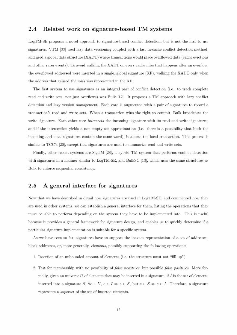
2.4 Related work on signature-based TM systems

LogTM-SE proposes a novel approach to signature-based conflict detection, but is not the first to use

signatures. VTM [33] used lazy data versioning coupled with a fast in-cache conflict detection method,

and used a global data structure (XADT) where transactions would place overflowed data (cache evictions

and other rarer events). To avoid walking the XADT on every cache miss that happens after an overflow,

the overflowed addressed were inserted in a single, global signature (XF), walking the XADT only when

the address that caused the miss was represented in the XF.

The first system to use signatures as an integral part of conflict detection (i.e. to track complete

read and write sets, not just overflows) was Bulk [12]. It proposes a TM approach with lazy conflict

detection and lazy version management. Each core is augmented with a pair of signatures to record a

transaction’s read and write sets. When a transaction wins the right to commit, Bulk broadcasts the

write signature. Each other core intersects the incoming signature with its read and write signatures,

and if the intersection yields a non-empty set approximation (i.e. there is a possibility that both the

incoming and local signatures contain the same word), it aborts the local transaction. This process is

similar to TCC’s [20], except that signatures are used to summarize read and write sets.

Finally, other recent systems are SigTM [28], a hybrid TM system that performs conflict detection

with signatures in a manner similar to LogTM-SE, and BulkSC [13], which uses the same structures as

Bulk to enforce sequential consistency.

2.5 A general interface for signatures

Now that we have described in detail how signatures are used in LogTM-SE, and commented how they

are used in other systems, we can establish a general interface for them, listing the operations that they

must be able to perform depending on the system they have to be implemented into. This is useful

because it provides a general framework for signature design, and enables us to quickly determine if a

particular signature implementation is suitable for a specific system.

As we have seen so far, signatures have to support the inexact representation of a set of addresses,

block addresses, or, more generally, elements, possibly supporting the following operations:

1. Insertion of an unbounded amount of elements (i.e. the structure must not “fill up”).

2. Test for membership with no possibility of false negatives, but possible false positives. More for-

mally, given an universe U of elements that may be inserted in a signature, if I is the set of elements

inserted into a signature S, ∀e ∈ U , e ∈ I ⇒ e ∈ S, but e ∈ S ; e ∈ I. Therefore, a signature

represents a superset of the set of inserted elements.

12

Mechanism Insert Test Intersect Union Clear Test if clear

Eager conflict detection X X X

Lazy (on-commit) conflict detection X X X X

LogTM-SE style thread suspension/migration X

Table 2.1: Required operations for a signature, depending on the primitive to be supported

3. Approximate set intersection: Two signatures S1 and S2 may need to be intersected, such that

∀e ∈ U , (e ∈ S1) ∧ (e ∈ S2) ⇒ e ∈ S1 ∩ S2.

4. Approximate set union: Two signatures S1 and S2 may need to be joined, such that ∀e ∈ U ,

(e ∈ S1) ∨ (e ∈ S2) ⇒ e ∈ S1 ∪ S2.

5. Clearing: A signature may need to be set into a state where no elements are represented in it, that

is, a cleared signature must represent the empty set exactly.

6. Test if clear: Finally, a signature may need to have a way to test whether it represents any elements.

This is typically done to check if the intersection of two signatures yields an empty set, so it may

performed in conjunction with the intersection operation.

Table 2.1 gives the required subset of operations that need to be implemented by a signature depending

on the mechanisms that need to be supported in a signature system. Note that future mechanisms may

require to implement additional operations not described here.

13

Chapter 3

Evaluation methodology

In chapters 4 to 6, different signature designs are explained and analyzed, and it is best to evaluate their

impact on the TM system just as they are described instead of deferring their evaluation until later. Now

that LogTM-SE and its signature-based conflict detection scheme have been described, we explain the

evaluation methodology that will be used in the performance evaluation.

3.1 System configuration

In chapters 4 to 6, the simulated system will be a 32-core CMP with simple in-order, single-issue cores.

Each core has split data and instruction 4-way set-associative caches of 32KB each. The cores share an

8-way, 8-banked L2 cache of 8MB. The system uses a MESI broadcast coherence protocol and a high-

bandwidth crossbar that connects the cores with the L2 banks. The system organization and parameters

are summarized in Figure 3.1.

Core 0

Core 31

Crossbar

L2 Bank 0

L2 Bank 7

Memory controller

Memory controller

...

...

Memory controller

Memory controller

Cores 32-way CMP, IPC/core=1, SPARCv9 ISA

L1 Caches 32KB split,4-way associative,64B lines, 3-cycle access latency

L2 Cache 8MB, 8-way assoc., 8-banked, 64B lines,6/20-cycle tag/data access latency

Coherence MESI, snooping,protocol signature checks broadcasted by L2

Memory 4 memory controllers,subsystem 450-cycle latency to main memory

Interconnect Crossbar, 5-cycle link latency

(a) System organization (b) System parameters

Figure 3.1: Simulated system

14

3.2 Simulation methodology

The simulations have been performed using the Simics full-system simulator, augmented with the Wis-

consin Multifacet GEMS [27] toolset to model the memory subsystem and LogTM-SE accurately. Simics

is used to perform functional simulation of processor cores with a SPARCv9 ISA, running an unmodified

Solaris 9. All the effects of the OS (such as page faults and system calls) are taken into account in the

simulation. The HTM interface is implemented via magic calls, special no-ops that Simics detects and

passes to the memory model. Memory access latency is slightly perturbed in each simulation, and all

the results presented are averaged across multiple runs to address variability issues [1].

3.3 Workloads

To evaluate the performance impact of different signature designs in LogTM-SE, we use five different

benchmarks with interesting and varying behaviors relevant to the evaluation of signatures:

• Btree: In this microbenchmark, each thread accesses a shared B-tree to perform either a lookup

or an insertion (with 80%/20% probabilities) using transactions. Per-thread memory allocators are

used for performance.

• Raytrace and Barnes: Both workloads have been taken from the SPLASH-2 suite [44]. The

original versions of the SPLASH-2 workloads featured fine-grained synchronization, and, conse-

quently, their transactionalized versions [30] have relatively small transactions with a typically

small amount of contention. Raytrace and Barnes have been selected from these because they are

the two that exert more pressure on signature designs. Raytrace performs 3D scene rendering using

ray tracing, and Barnes simulates the interaction of a system of N bodies in discrete time-steps,

using the Barnes-Hut method.

• Vacation and Delaunay: These benchmarks have been selected from the STAMP benchmark

suite [28]. Both feature coarse-grain, long-running transactions with large read and write sets, and

follow TCC’s model of all transactions, all the time [20]. Consequently, these are the benchmarks

that exert the most pressure on the signatures. Vacation models a travel reservation system that

uses an in-memory database implemented using trees, and is similar in design to the SPECjbb2000

workload. Delaunay implements Delaunay mesh generation algorithm, which generates guaranteed-

quality meshes.

The exact parameters and inputs of the benchmarks can be found in Table 3.1. Their main TM-related

characteristics are summarized quantitatively in Table 3.2, and qualitatively in Table 3.3.

15

Benchmark Input Units of work

btree Uniform random 100000 operations

raytrace teapot 1 parallel phase

barnes 512 bodies 1 parallel phase

vacation n8-q10-u80-r65536-t4096 4096 operations

delaunay gen4.2 -

Table 3.1: Parameters of the benchmarks

Benchmark Time in Read set Write set Dyn. instrs / Retries /transactions size (avg/max) size (avg/max) xact (avg/max) xact

btree 54.9% 13.2 / 20 0.64 / 15 514.0 / 1988 0.022raytrace 2.7% 5.25 / 573 1.98 / 4 11.8 / 18406 0.003barnes 9.2% 5.23 / 41 3.92 / 35 200.7 / 3493 0.23

vacation 100% 80.4 / 176 12.4 / 62 4301 / 318624 2.05delaunay 100% 26.2 / 222 14.8 / 131 8331 / 89105 1.29

Table 3.2: Quantitative TM characterization of the benchmarks

3.4 Metrics

When presenting simulation results, we will mainly focus on the impact that each signature design has

on performance measured in terms of execution time. To abstract from system-related parameters, these

times are normalized to the execution time of a system with “perfect” signatures, i.e. signatures that

have no false positives or false negatives, and have a single-cycle access time. A perfect signature is not

implementable in bounded hardware, but provides an upper bound on conflict detection capabilities.

Benchmark Time in Amount of Read set Write-set Transactiontransactions contention size size length

btree high low medium small mediumraytrace low low small-large small short-longbarnes low high small small medium

vacation high high large medium longdelaunay high high large medium long

Table 3.3: Qualitative TM behavior of the benchmarks

16

Chapter 4

Bloom signatures

All currently proposed TM systems that use hardware signatures advocate implementing them with

Bloom filters. Therefore, our first step in the study of signatures is to present, analyze, and evaluate the

area requirements and the performance of these structures. We start with the description and analysis of

two different implementations of Bloom signatures: true and parallel Bloom signatures, and show that

they are equivalent when testing for membership is used. This is an important result, because parallel

Bloom signatures require single-ported memories instead of multi-ported ones, and the same total state

as true Bloom signatures, and so are much more area-efficient. We then overview some results on the

optimality of Bloom signatures, discuss related work, and present the area and performance evaluations.

4.1 True Bloom signatures

We call a signature implemented with a single Bloom filter a true Bloom signature. Here we review

true Bloom signatures, analyze their false positive rates, and sketch a hardware implementation using

multi-ported SRAMs.

4.1.1 Design

A true Bloom signature provides an efficient way to represent a set of values (in our case, block addresses).

Adding new addresses to the set is simple, and testing for membership is also easy, with a small probability

of false positives and no possibility of false negatives. A true Bloom signature consists of an m-bit field,

which is accessed using k independent hash functions, as shown in Figure 4.1a.

Every bit in the field is initially set to 0. To insert an address to the set, the k hash values of the

address are computed. Each hash function hi can give a value in the range [0, ...,m− 1]. The bits at the

positions indicated by these values are set to 1. To test for membership of an element, we compute the

17

0 1 0 1 .... 0 0 1 0

h 1 h 2 h k ...

Address

0 1 0 1 .... 0 0 1 0

h 1 h 2 h k ...

Address Add operation

Test operation

(a) Design

h 1

h 2

h k

...

bitlines

wordlines

k -ported SRAM

of m bits

Address

(b) Hardware implementation

Figure 4.1: True Bloom Signatures

results of the hash functions and check the contents of the bits they point to. The address is not in the

set if there is at least one bit not set. If all the bits are set to 1, either the address is in the set, or the

addition of other addresses caused these bits to be set to 1 and we are getting a false positive.

Additionally, it is easy to perform the approximate intersection or union of two signatures with

the requirements established in Section 2.5, provided that the two signatures have the same size and

hash functions. The intersection is performed by computing the bitwise AND of the bit-fields of both

signatures, while the union is computed by doing a bitwise OR of the bit-fields.

4.1.2 Analysis

We now present a formal analysis of false positives, which are critical to performance, when using test for

membership. Let us assume that we insert n addresses to the filter, and that the k-tuple of hash values

is independent and uniformly distributed. This is approximately the case even with practical address

streams if we use universal or almost-universal hash functions [35], as we will show in the performance

evaluation.

On a single insertion, the probability of a particular hash function writing a 1 to the i-th position

on the bit array (regardless of whether this position was 0 or 1) is 1/m. Since the k hash functions are

independent, the probability of not setting a certain bit to 1 in one insertion operation is (1 − 1/m)k.

Therefore, the probability of a single bit still being 0 after the n insertions is p0(n) = (1 − 1/m)nk.

On a test for membership, the test returns true only if all of the checked bits are set to one. The

probability of getting a positive match is therefore:

PP (n) = (1 − p0(n))k

However, we are interested in the probability of false positives, i.e. the probability that a hit occurs

and that the element that we test for is not one of the n inserted elements. By Bayes’ rule:

PFP (n) = Prob(Positive AND Address was not inserted before)

18

PFP (n) = PP (n) × Prob(Address was not inserted before | Test was positive) = PP (n) × PI(n)

where PI(n) is the probability that the address was not inserted into the signature, conditioned by a

positive test result in the signature. In general, PI(n) will depend on the locality of the address stream

and the accuracy of the signature. However, if the total number of elements that we can test for is

denoted by nt, and assuming that the elements we test for are independent of the inserted elements and

also uniformly distributed, this probability is PI(n) = nt−nnt

. Typically, the set of elements that we will

test for is much larger than the set of inserted elements, i.e. nt ≫ n (because the read/write sets of a

transaction are typically smaller than the working sets of the different threads in the system). Hence,

PI(n) =nt − n

nt

∼= 1

PFP (n) ∼= PP (n) = (1 − p0(n))k

Experimentally, however, the probability of a false positive may differ from the probability of a positive,

because addresses are not random and independent (e.g., locality) and hash functions might not be

perfectly universal [35, 34]. Nevertheless, we find this equation to be a good first-order approximation,

and at the very least this is an upper bound on the probability of false positives (because PI(n) ≤ 1).

Finally, we can apply an accurate approximation to simplify the expression of PFP (n). From the

Taylor series expansion of the exponential function,

ex =∞∑

n=0

1

n!xn = 1 + x +

x2

2+

x3

6+ ...

we can see that ex ∼= 1 + x when |x| ≪ 1. For our purposes, m is relatively large, so |1/m| ≪ 1 and:

e−1/m = 1 −1

m+

1

2m2−

1

6m3+ ... ∼= 1 −

1

m

Therefore, our formulas reduce to:

p0(n) = (1 − 1/m)nk ∼= e−nkm

PFP (n) ∼=(

1 − e−nkm

)k

In general, there are three design dimensions in a true Bloom signature:

1. The size of the bit field (m): A larger field decreases the probability of false positives for a

certain number of insertions (PFP (n)), independently of the other parameters of the signature.

However, increasing this parameter has a direct impact on the amount of area needed for the

19

signature, and, if signatures need to be transmitted, it will increase the bandwidth requirements

as well. Therefore, in order to design efficient and accurate signatures, we cannot just rely on

increasing the signature size.

2. The number of hash functions (k): In general, increasing the number of hash functions (larger

k), reduces the amount of false positives for small read/write sets (an important case) at the cost

of more false positives for large read/write sets. Figure 4.2 shows the probability of false positives

in 1024-bit true Bloom signatures as we vary the number of addresses inserted, n, on the x-axis,

for different numbers of hash functions, k. In the left-hand figure, n varies from 0 to 1000, while in

the right-hand figure it goes up to 120. For example, when n = 20 elements have been inserted, a

signature with k = 1 has PFP (n) = 0.02, and a signature with k = 4 has PFP (n) = 3× 10−5, while

for n = 800 elements, the probabilities are now 0.54 and 0.84, and the 1-hash function signature

outperforms the 4-hash function signature.

0 200 400 600 800 10000

0.1

0.2

0.3

0.4

0.5

0.6

0.7

0.8

0.9

1

n (# addresses inserted)

Pro

babi

lity

of fa

lse

posi

tives

Bloom filters, m=1024 bits, k=[1,2,4,8]

k=1k=2k=4k=8

0 20 40 60 80 100 1200

0.005

0.01

0.015

0.02

0.025


Pro

babi

lity

of fa

lse

posi

tives


k=1k=2k=4k=8

Figure 4.2: Influence of the number of hash functions on the probability of false positives of aBloom signature

3. The type of hash functions: If the addresses that we used for insertions and membership tests

were statistically independent and uniformly distributed, the hash functions used would be of little

importance in a signature design. However, in real programs this is far from the actual situation:

memory accesses are clustered to specific regions of memory, and successive addresses are highly

correlated, due to the phenomenons of spatial and temporal locality. The goal of the k different

hash functions is to obtain hash values with a distribution somewhat close to the uniform, and

to achieve a low correlation between the k hash values generated each time. Bit-selection (i.e.

using a subset of the bits of the address as a hash value, as shown in Figure 4.3a) has been the

approach used so far in the proposed TM systems. While bit-selection is simple, it may not yield

sufficient variation to approximate a good hash function. However, we cannot afford to implement

complex hash functions because of the limited hardware requirements. Instead, we will settle for a

20

middle ground: we will consider using H3 hash functions [10, 35], which approximate universal hash

functions better than bit-selection and can achieve many uncorrelated and uniformly distributed

hash values. In a H3 hash function, each bit of each hash value is generated by XORing a subset of

the bits of the address, as shown in Figure 4.3b. These address bits are randomly chosen, with the

probability of selecting each individual address bit being 0.5. In this paper we follow the definition

of the H3 hash functions closely, but actual implementations could explore XORing fewer address

bits to reduce hardware cost. The issue of XOR-based hash functions was explored in detail by

Vandierendonck and De Bosschere [42], who provide and explain meaningful metrics to facilitate

an efficient design of these functions.

Address bits

H 0 H 1

...

(a) Bit-selection (bit-interleaving)

Address bits

Hash bits

(b) Hardwired H3

Figure 4.3: Considered types of hash functions

4.1.3 Implementation

True Bloom signatures can be implemented in hardware by partitioning the bit field into words, and

storing them in a small, bit-addressable SRAM. To do this, we divide the output bits of the generated

hash values: some of them are used to control the wordlines, while the others drive the bitlines, as shown

in Figure 4.1b. To insert an address, for each hash value, the appropriate wordline is raised, and the

corresponding bitline is driven to high, while the other bitlines are left floating. To test for an address,

the bit addressed by each hash value is read by raising the appropriate wordline and sensing the value

at the bitline.

To implement k hash function signatures, we need k read and write ports in the SRAM. This is not

area-efficient for filters with multiple hash functions, since the size of an SRAM cell increases quadratically

with the number of ports. In the next section, we describe a partitioning strategy to overcome this

quadratic growth. Regarding the hash functions, bit-selection requires no hardware at all, and hardwired

H3 hash functions are relatively inexpensive to implement, requiring a small tree of 2-input XOR gates

per bit of each hash function.

21

4.2 Parallel Bloom signatures

This section develops parallel Bloom signatures, which perform like true Bloom signatures, but avoid

using multi-ported SRAMs.

4.2.1 Design

Instead of having a single k-hash function Bloom filter, we now consider using k Bloom filters, each with

a different hash function. To keep the amount of state the same, each of the Bloom filters uses a m/k-bit

field. On an insertion, we hash the address and set a bit in all k filters, and report that an address

is represented in the signature only if all the individual Bloom filters say so. We call this structure a

parallel Bloom signature; its design is shown in Figure 4.4a. A similar design was proposed in Bulk [12].

h 1 h 2 h k ...

Address Address Add operation

Test operation

0 1 .... 0 1 0 .... 0 0 0 .... 1 ...

h 1 h 2 h k ...

0 1 .... 0 1 0 .... 0 0 0 .... 1 ...

(a) Design

h 1 h 2 h k ...

Address

...

k single-ported SRAMs of m/ k bits


Figure 4.4: Parallel Bloom Signatures

4.2.2 Analysis

As in the analysis of true Bloom signatures, let us assume that we insert that the hash functions generate

independent, uniformly distributed hash values. If we insert n addresses, the probability of a bit in the

i-th filter being still 0 is p0(n) =(

1 − 1m/k

)n

.

When we test for membership, a match is only reported if a positive match happens in all the filters.

Hence,

PFP (n) ∼= PP (n) = (1 − p0(n))k

This expression is different from the PFP (n) of a true Bloom signature. However, if we apply the

Taylor series approximation we described in Section 4.1.1 again, we obtain:

k

m≪ 1 ⇒ 1 −

1

m/k∼= e−

km

And therefore,

PFP (n) ∼=(

1 − e−nkm

)k

22

Under the approximation, a parallel Bloom signature achieves the same PFP (n) as a true Bloom

signature. This approximation is very good when the number of hash functions is much smaller than

the length of the bit field (i.e. k/m ≪ 1), which will normally be the case. This approximation will be

verified in an experimental setting in Section 4.6. A similar approximation was also used in filters in

networking [17], but without realizing that one hash function per parallel filter is sufficient and can lead

to a more area-efficient design.


In terms of hardware, the equivalence presented in the previous sections means that, instead of im-

plementing multi-hash function Bloom signatures with multi-ported large SRAMs, we can use multiple

smaller single-ported SRAMs. Finally, the hash functions are also slightly less expensive to implement,

because they now generate hash values that are smaller by a factor of k. Figure 4.4b shows a canonical

hardware implementation.

4.3 The optimality of Bloom filters

An interesting question that deserves some analysis is how space-efficient Bloom signatures are. This

matter is of interest for two reasons: reducing the hardware requirements by choosing an efficient Bloom

filter configuration, and reducing the bandwidth requirements for systems where signatures need to

be transmitted. For a fixed number of additions and a fixed size, the probability of false positives is

minimized for:

k = kopt∼=

m

nln(2)

(this formula is obtained by differentiating PFP (n) with respect to k and finding where if becomes

0). This means that, if we knew the number of elements to be inserted in advance, we could choose the

optimal number of hash functions. This is a typical setting in software applications, but not in signatures:

first, we do not know the number of block addresses to be inserted in advance, and second, signature

tests and insertions are interleaved. The bottom line is that varying the parameters of the Bloom filter

dynamically to reduce the probability of false positives is not trivial. In Chapter 6, however, we explore

the possibility of adapting the number of hash functions by predicting the size of the read and write sets

of a transaction.

When discussing space-efficiency, it is useful to see how close we are to the information-theoretical

lower bound. In the case of Bloom signatures, Carter et al. have shown that the minimum amount of

information to represent an arbitrary set of n elements with no false negatives and false positives is [11]:

23

mopt = n · log2

(

1

PFP

)

, provided that PFP ≪ 1.

This proof is obtained using arguments from Kolmogorov complexity, which deals with the amount of

information of individual objects1. Interested readers may consult the proof at [11]. Using this formula,

we can see that a Bloom filter is used with the optimal number of hash functions,

PFP (n) ∼=(

1 − e−nkopt

m

)kopt

=

(

1

2

)mn

ln(2)

mopt = n · log2(2mn

ln(2)) = nm

nln(2) = m · ln(2) ⇒ m ∼= 1.44mopt

i.e., we are using 44% more space than what the theoretical lower bound imposes.

To get closer to the theoretical lower bound, two alternatives have been explored: compression and

hash-based implementation of Bloom filter-like structures. Mitzenmacher has a complete study in com-

pressed Bloom filters [29]. An important corollary that can be extracted from his findings is that com-

pression enables us to be close to the lower bound across all the utilization factors of the Bloom filter.

Compression has been proposed in Bulk [12] (specifically, run-length encoding), in which transactions

broadcast write-set signatures on commit, to reduce the bandwidth requirements. However, compression

is an inherently serial operation on the bits of the signature, and even sophisticated implementations may

take several tens or hundreds of cycles to compress and decompress a reasonably-sized signature (e.g. of

around 2Kbits). In Bulk, this introduces an undesirable high latency in the common commit operation.

Additionally, compression is not interesting if we just want to reduce the hardware requirements.

An interesting result of the lower bound presented before is that, if we seek to achieve PFP = 2−r,

simply using a hash function with r bits and keeping the n hash values of the inserted addresses in a

data structure requires n · r = n · log2

(

1PF P

)

bits, so it is optimal in terms of space (assuming that

we seek an accurate representation, i.e. PFP ≪ 1). Pagh et al. have proven the existence of a data

structure that allows insertions and tests in constant time [31], and Bonomi et al. present a hash-table-

based design amenable to hardware implementation that outperforms Bloom filters at low loads [7]. The

problem with these structures is that the amount of elements that we can represent is bounded by the

size of the memory used. This is not acceptable for signatures, which must be capable to represent an

unbounded amount of elements in a bounded amount of space. In the next two chapters, we present novel

implementations of signatures that overcome this problem by using hashing at low loads and morphing

into a Bloom filter at high loads.

1By contrast, classical Information Theory deals with the amount of information of a random variable, and is of littleuse to us.

24

4.4 Related work on Bloom filters

Bloom filters were first proposed in 1970 by Burton H. Bloom [4]. Many variations and alternative

implementations of the original scheme have been proposed since then. Counting Bloom filters associate

a counter to each position of the bit-field, to allow deletions [18] or to represent multisets. Bloomier

filters adapt Bloom filters to build an associative map [14]. Spectral Bloom filters also extend Bloom

filters to represent multisets [15].

Bloom filters have been used in computer architecture for purposes other than conflict detection in

Transactional Memory (e.g., for load-store queues [39] and early miss detection in L2 caches [19]).

Hardware implementations of Bloom filters are common in network applications. Broder and Mitzen-

macher have a survey paper on the theory and applications of Bloom filters in networks [9]. Dharma-

purikar et al. describe a packet inspection system with hardware-implemented Bloom filters [17]. Often,

these designs require counting Bloom filters, so efficient hardware implementations [36] and alternative

structures [8] have been proposed.

The choice of hash functions in hardware Bloom filters is crucial, because complex functions may

achieve better performance, but take more area. Ramakrishna et al. [35] compare bit-selection, simple

XORing and H3 for address hash tables with real-life data, and conclude that only H3 functions can

achieve analytical performance in practice. Earlier work by Ramakrishna [34] shows how we can achieve

analytical performance with Bloom filters in a practical setting by using a universal hash function. The

H3 family of hash functions was first described by Carter and Wegman [10]. This hash function family

is part of the more generic type of XOR-based hash functions. Vandierendonck and De Bosschere [42]

describe two approaches to measure and improve the quality of specific XOR-based hash functions.

4.5 Area evaluation

So far, we have described and analyzed true and parallel Bloom signatures. In this section, we use

CACTI [41] to estimate and compare the area requirements of both designs. We also study the area

overheads of Bloom signatures in real systems.

4.5.1 True and parallel Bloom signatures

Table 4.1 compares the area required by true and parallel Bloom signatures for a 4Kbit signature. The

area estimates were obtained using CACTI 4.2 [41], for a technology node of 65nm, and one to four hash

functions. We used memories with 8-byte words, which yield memories of the same wordlines and bitlines

for the true Bloom signature. We use no single-ended read ports, and separate read/write ports. For true

Bloom signatures, we used k-ported SRAMs, and for parallel Bloom signatures we used single-ported

25

SRAMs.

As we can see, parallel Bloom filters are significantly more area efficient than true Bloom filters,

providing area savings of 3.2× for two hash functions, and of 8× for four hash functions. We expect

a quadratic savings in area proportional to the reduction in number of ports. However, due to the

relatively small size of SRAMs, the fixed overheads, like multiplexers and sense amps, reduce the area

savings achieved by reducing number of ports.

k 1 2 4True Bloom 0.031 0.113 0.279

Parallel Bloom 0.031 0.032 0.035

Table 4.1: SRAM area requirements (in mm2) of true and parallel Bloom signatures, m=4Kbit, 65nmtechnology.

In addition to the SRAMs, the other main contribution to area is the hash functions. While bit-

selection requires no additional hardware, the H3 hash functions require additional area for the XOR

gates that implement the hash functions. Recall from Section 4.1.1 that, for n-bit addresses we need a

tree of about n/2 2-input XOR gates for each bit of the hash function. This circuit can be optimized

for area and delay by doing full layout, but such implementation is beyond the scope of this analysis.

Furthermore, more area-efficient hash functions can be constructed by XORing together fewer bits . In

this report, we provide an area estimate assuming a n/2 XOR tree. Table 4.2 shows the number of

2-input XOR gates required for implementing the H3 hash functions in a 4Kbit signature. In terms of

transistor count, assuming a 4-transistor XOR gate design [43], for k = 4, the hash functions occupy

about 20% of the size of the SRAM.

k 1 2 4True Bloom 180 360 720

Parallel Bloom 180 330 600

Table 4.2: Number of XOR gates required by true and parallel Bloom signatures using H3 hash functions,m=4Kbit.

4.5.2 Bloom signatures in real systems

To understand the area overheads of adding transaction support to hardware, we selected two very

different multi-core systems: the Sun Niagara [23], which uses simple in-order cores, and the AMD

Barcelona [46], which uses complex out-of-order cores. While signatures are not the only extra hardware

required for transaction support, in this study we focus on the area overheads of signatures alone. To

make the analysis simple we chose one signature design: parallel Bloom signatures of 4Kbits with four

hash functions, using the bit-selection hash functions (or using any other kind of hash function without

taking into account its area overhead). We assume separate signatures per thread context, and separate

26

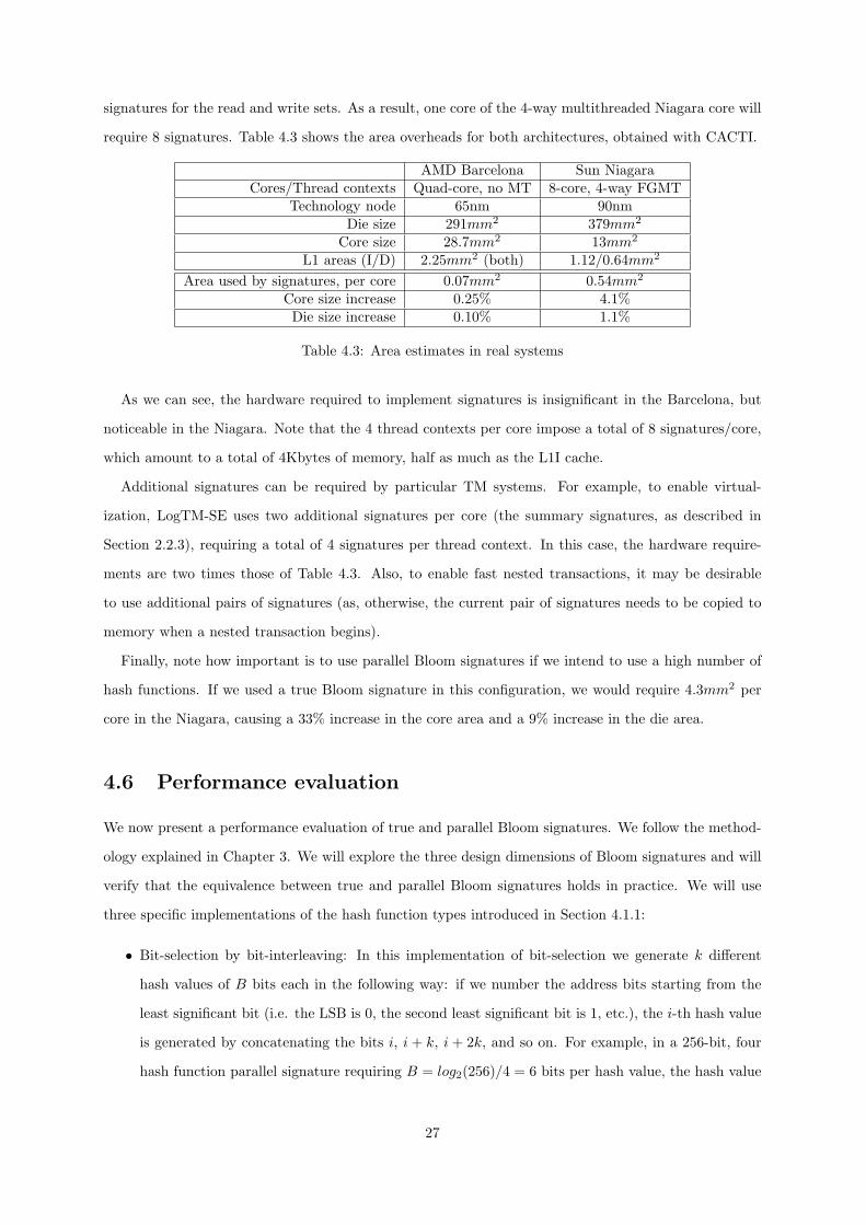
signatures for the read and write sets. As a result, one core of the 4-way multithreaded Niagara core will

require 8 signatures. Table 4.3 shows the area overheads for both architectures, obtained with CACTI.

AMD Barcelona Sun NiagaraCores/Thread contexts Quad-core, no MT 8-core, 4-way FGMT

Technology node 65nm 90nmDie size 291mm2 379mm2

Core size 28.7mm2 13mm2

L1 areas (I/D) 2.25mm2 (both) 1.12/0.64mm2

Area used by signatures, per core 0.07mm2 0.54mm2

Core size increase 0.25% 4.1%Die size increase 0.10% 1.1%

Table 4.3: Area estimates in real systems

As we can see, the hardware required to implement signatures is insignificant in the Barcelona, but

noticeable in the Niagara. Note that the 4 thread contexts per core impose a total of 8 signatures/core,

which amount to a total of 4Kbytes of memory, half as much as the L1I cache.

Additional signatures can be required by particular TM systems. For example, to enable virtual-

ization, LogTM-SE uses two additional signatures per core (the summary signatures, as described in

Section 2.2.3), requiring a total of 4 signatures per thread context. In this case, the hardware require-

ments are two times those of Table 4.3. Also, to enable fast nested transactions, it may be desirable

to use additional pairs of signatures (as, otherwise, the current pair of signatures needs to be copied to

memory when a nested transaction begins).

Finally, note how important is to use parallel Bloom signatures if we intend to use a high number of

hash functions. If we used a true Bloom signature in this configuration, we would require 4.3mm2 per

core in the Niagara, causing a 33% increase in the core area and a 9% increase in the die area.

4.6 Performance evaluation

We now present a performance evaluation of true and parallel Bloom signatures. We follow the method-

ology explained in Chapter 3. We will explore the three design dimensions of Bloom signatures and will

verify that the equivalence between true and parallel Bloom signatures holds in practice. We will use

three specific implementations of the hash function types introduced in Section 4.1.1:

• Bit-selection by bit-interleaving: In this implementation of bit-selection we generate k different

hash values of B bits each in the following way: if we number the address bits starting from the

least significant bit (i.e. the LSB is 0, the second least significant bit is 1, etc.), the i-th hash value

is generated by concatenating the bits i, i + k, i + 2k, and so on. For example, in a 256-bit, four

hash function parallel signature requiring B = log2(256)/4 = 6 bits per hash value, the hash value

27

H0 is be generated with bits (0, 4, 8, 12, 16, 20), and H3 is generated with bits (3, 7, 11, 15, 19, 23). If

the number of bits required for the hash functions is greater than the number of bits of the address

we want to consider, we wrap around and start selecting bits from the beginning again. In our

case, we only use the 25 least significant bits of the address: we do not want to consider complete

addresses, since higher-order bits usually have a very small variation. For example, in a 2048-bit,

4 hash function parallel Bloom signature, requiring B = 9 bits, we would get H1 with the address

bits (1, 5, 9, 13, 17, 21, 0, 4, 8).

• Fixed H3 hash functions: In this case, the bits of the address that are XORed to generate each

bit of the hash value are hardwired (i.e. cannot change), and every thread context in the system

implements the same hash functions. This enables an area-efficient implementation of the hash

functions.

• Variable H3 hash functions: With this flavor of H3 functions, the subset of bits chosen to generate

each bit of the hash value are randomly selected after each commit on abort. This causes the hash

functions in the system to be different from each other and to be constantly changing. This increases

the area requirements and the complexity of the hash functions, but the variability mitigates the

problems that having the same signature aliases between certain pairs of addresses all the time

may introduce. For example, suppose that we have two shared variables in our program, one which

is widely shared and other which is sometimes modified. If the addresses of two variables map

to the same bits in the signature (i.e. there is an alias between them), the second one will be

very difficult to modify because it will be typically reported as read by other transactions in the

signature checks. This may introduce a significant performance impact if the hash functions are

fixed, but not if they constantly change.

Table 4.4 shows the execution times normalized to a perfect signature for different configurations.

Each individual graph shows how the performance varies with the signature size (256 to 2048 bits, in the

x-axis) and the number of hash functions (different lines in each graph). Both true and parallel Bloom

signatures are represented in the same graph (with dashed and solid lines, respectively). Each row of

graphs shows the result from a single benchmark, using a different type of hash functions in each graph

of the row (bit-selection, fixed H3, and variable H3). We now comment on the different aspects of these

results.

4.6.1 True vs. Parallel Bloom signatures

Using probabilistic analysis, we previously saw that true and parallel Bloom signatures should perform

equivalently. Looking at the results, we can see how the differences are generally quite small when using

28

Legend

BitSel, k=1 BitSel, k=2, True BitSel, k=2, Parallel BitSel, k=4, True BitSel, k=4, Parallel

Fixed H3, k=1 Fixed H

3, k=2, True Fixed H

3, k=2, Parallel Fixed H

3, k=4, True Fixed H

3, k=4, Parallel

Var. H3, k=1 Var. H

3, k=2, True Var. H

3, k=2, Parallel Var. H

3, k=4, True Var. H

3, k=4, Parallel

Bit-selection Fixed H3 Variable H3

btr

ee

256 512 1024 2048

1

1.2

1.4

1.6

1.8

2

2.2

2.4

2.6

2.8

3

Signature size

Exe

cutio

n tim

e (n

orm

aliz

ed to

Per

fect

)

256 512 1024 2048

1

1.2

1.4

1.6

1.8

2

2.2

2.4

2.6

2.8

3

Signature size

Exe

cutio

n tim

e (n

orm

aliz

ed to

Per

fect

)

256 512 1024 2048

1

1.2

1.4

1.6

1.8

2

2.2

2.4

2.6

2.8

3

Signature size

Exe

cutio

n tim

e (n

orm

aliz

ed to

Per

fect

)

raytr

ace

256 512 1024 2048

1

1.1

1.2

1.3

1.4

1.5

1.6

Signature size

Exe

cutio

n tim

e (n

orm

aliz

ed to

Per

fect

)

256 512 1024 2048

1

1.1

1.2

1.3

1.4

1.5

1.6

Signature size

Exe

cutio

n tim

e (n

orm

aliz

ed to

Per

fect

)

256 512 1024 2048

1

1.1

1.2

1.3

1.4

1.5

1.6

Signature size

Exe

cutio

n tim

e (n

orm

aliz

ed to

Per

fect

)

bar

nes

256 512 1024 20480.98

1

1.02

1.04

1.06

1.08

1.1

Signature size

Exe

cutio

n tim

e (n

orm

aliz

ed to

Per

fect

)

256 512 1024 20480.98

1

1.02

1.04

1.06

1.08

1.1

Signature size

Exe

cutio

n tim

e (n

orm

aliz

ed to

Per

fect

)

256 512 1024 20480.98

1

1.02

1.04

1.06

1.08

1.1

Signature size

Exe

cutio

n tim

e (n

orm

aliz

ed to

Per

fect

)

Continued on next page...

29

Bit-selection Fixed H3 Variable H3va

cati

on

256 512 1024 20481

2

3

4

5

6

7

8

Signature size

Exe

cutio

n tim

e (n

orm

aliz

ed to

Per

fect

)

256 512 1024 20481

2

3

4

5

6

7

8

Signature size

Exe

cutio

n tim

e (n

orm

aliz

ed to

Per

fect

)

256 512 1024 20481

2

3

4

5

6

7

8

Signature size

Exe

cutio

n tim

e (n

orm

aliz

ed to

Per

fect

)

del

aunay

256 512 1024 20481

2

3

4

5

6

7

Signature size

Exe

cutio

n tim

e (n

orm

aliz

ed to

Per

fect

)

256 512 1024 20481

2

3

4

5

6

7

Signature size

Exe

cutio

n tim

e (n

orm

aliz

ed to

Per

fect

)

256 512 1024 20481

2

3

4

5

6

7

Signature size

Exe

cutio

n tim

e (n

orm

aliz

ed to

Per

fect

)Table 4.4: Execution times for different true (dashed lines) and parallel Bloom signatures (solid lines).

fixed or variable H3 hash functions (typically the discrepancies are of 2% or less). The highest difference

for H3, 17%, occurs for raytrace, with 512-bit signatures and four fixed H3 hash functions. However,

performance differences between true and parallel Bloom signatures are much higher for bit-selection

than for H3 hash functions, especially when using four hash functions. Note how these differences are

of up to 100% in vacation and delaunay. These results are a direct consequence of the hash function

quality: the H3 hash functions create more uniform and uncorrelated distributions of the hash values

than bit-selection, and therefore are closer to our theoretical model of a Bloom filter.

From the experiments, we can safely conclude that, even though the conditions required in the the-

oretical analysis are not strictly met in practice, the equivalence of true and Parallel Bloom signatures

still holds, given that good enough hash functions are used.

4.6.2 Effect of signature size

We can see that doubling the signature size generally produces a noticeable performance gain. Perhaps

surprisingly, at times, increasing the signature size results in lower performance (e.g. in raytrace, the

execution time increases by 13% when going from 256 to 512 bits in a parallel Bloom signature with two

fixed H3 hash functions). This is an artifact of the the LogTM-SE system and the underlying complex

30

interactions in the memory system and between transactions. For example, aborts resulting from a false

positive at times mask an expensive abort that would occur later if this false positive was not triggered.

The same behavior has been observed in other signature-based TM systems [28].

4.6.3 Effect of the number and type of hash functions

Bit-selection vs. fixed H3: In Table 4.4, we can clearly appreciate that the type of hash functions

used may be more important than the number of them. Focusing on the differences between bit-selection

and fixed H3, we see that both types of functions perform comparably for raytrace and barnes, while for

the more demanding btree, vacation, and delaunay (which spend most or all their time in transactions),

bit-selection hash functions are consistently surpassed by their H3 counterparts: even 2Kbit signatures

produce a significant degradation (20%-50%) in the execution time of these three benchmarks when

bit-selection is used. However, 2Kbit signatures using four H3 hash functions produce no degradation in

vacation or delaunay, and even 256-bit signatures perform well in btree. But perhaps the most significant

result is that increasing the number of hash functions from two to four when using bit-selection does

not help performance, but generally hurts it (with the exception of raytrace). This result is consistent

with the findings presented in the Bulk paper [12], in which bit-selection is used, and it is concluded

that using more than two hash functions yields worse performance. In contrast, increasing the number

of H3 hash functions from two to four always entails better performance for a given size. Again, this is

due to the more uniformly distributed and uncorrelated hash values that the different H3 hash functions

generate.

Fixed vs. variable H3: If we now focus on the differences between using fixed or variable H3 hash

functions, we can see that variable H3 achieve excellent results in btree and raytrace, while vacation and

delaunay exhibit similar results for both hash function types. Recall that the objective of using variable

hash functions was to avoid repeated false positives over time, because, as the hash functions change,

the aliases between different addresses change as well. It is also remarkable that, for btree and raytrace

(which have typically small read and write sets), the difference between the number of hash functions

used becomes negligible. The number of hash functions is still determinant in vacation and delaunay,

which have larger read and write sets.

Using more than four hash functions: Finally, we also performed experiments using eight fixed

H3 hash functions (not shown in the graphs for clarity), which show that using eight hash functions

yields similar results than using four. Performance is marginally better for btree, barnes and delaunay,

and slightly worse for raytrace and vacation (about 10% worse, depending on the particular situation). If

we had to decide the number of hash functions to implement based on these results, we would probably

31

choose to use four over (mainly due to their simpler implementation), but it is good to know that the

performance degradation is not terrible if we use more hash functions than necessary if we use H3, as it

happens when using bit-selection.

Based on these experiments, if Bloom signatures with fixed hash functions are to be employed, it is

clear that about four hash functions should be used, either from the H3 family or from a similarly good

one that allows us to have a high number of uncorrelated hash functions, instead of using a low number

of hash functions and simple bit-selection. If the system allows to have signatures with hash functions

that can change over time, it may be desirable to implement some form of inexpensive variable hash

functions to reap the benefits of variability.

4.6.4 Statistical analysis of the hash functions

Over the previous sections, we have based some of our explanations of the differences between the hash

function types on the statistical properties that hash values exhibit. Now, we substantiate our claims

with actual statistical data from the hash value distributions.

Figure 4.5 compares the hash value distributions of inserted addresses for two different benchmarks:

btree, which has small read and write sets, and vacation, which has large read and write sets. These

distributions were obtained by profiling the hash values of the elements that were inserted into the

signatures. The results correspond to the first hash function of a 512 bit, 2 hash function parallel Bloom

signature. Note the different ranges used in the y-axis across hash functions.

We can clearly see that the hash value distributions that bit-selection produce are very far from an

uniform one. For example, almost half of the insertions in btree map to the same place. The fixed H3

are much closer: they typically have a mean and standard deviation within 3% of those of an uniform

distribution, but have spikes due to the existence of more commonly accessed addresses. Finally, the

variable H3 achieve a truly uniform distribution over time, thanks to the continuous changes of the hash

functions. Note that, when larger address sets are used, both bit-selection and H3 generate distributions

with less spikes.

Since one of the main assumptions in the analysis of Bloom signatures was that the set of generated

hash values was independent and uniformly distributed, how close the distribution of hash values is from

the uniform has a great impact in how close are the simulated signatures from the theoretical discussion.

Note, however, that having variable H3 hash functions does not entail that the signatures are going to

perform as predicted by theory, as the set of inserted addresses each time still has a significant correlation.

Nevertheless, the effect of having variable hash functions is that the aliases caused by signatures vary

over time, and so avoid pathological conditions (e.g. making it difficult to write to a certain address

because there is a constant alias with the address of a widely shared variable).

32

0 50 100 150 200 2500

0.05

0.1

0.15

0.2

0.25

0.3

0.35

0.4

0.45

0.5

Hash value

Fra

ctio

n of

add

ed a

ddre

sses

(a) btree, BitSel

0 50 100 150 200 2500

0.01

0.02

0.03

0.04

0.05

0.06

0.07

0.08

0.09

0.1

Hash value

Fra

ctio

n of

add

ed a

ddre

sses

(b) btree, fixed H3

0 50 100 150 200 2500

0.01

0.02

0.03

0.04

0.05

0.06

0.07

0.08

0.09

0.1

Hash valueF

ract

ion

of a

dded

add

ress

es

(c) btree, var. H3

0 50 100 150 200 2500

0.05

0.1

0.15

0.2

0.25

Hash value

Fra

ctio

n of

add

ed a

ddre

sses

(d) vacation, BitSel

0 50 100 150 200 2500

0.01

0.02

0.03

0.04

0.05

0.06

0.07

0.08

0.09

0.1

Hash value

Fra

ctio

n of

add

ed a

ddre

sses

(e) vacation, fixed H3

0 50 100 150 200 2500

0.01

0.02

0.03

0.04

0.05

0.06

0.07

0.08

0.09

0.1

Hash value

Fra

ctio

n of

add

ed a

ddre

sses

(f) vacation, var. H3

Figure 4.5: Hash value distribution of inserted elements for a 512-bit parallel Bloom signature of 2 hashfunctions

33

Chapter 5

Cuckoo-Bloom signatures

So far, we have only considered signatures implemented with Bloom filters. In this chapter, we present

a novel signature implementation, called Cuckoo-Bloom signatures, inspired by cuckoo hashing. Cuckoo-

Bloom signatures match the low false positive rates of Bloom signatures with many hash functions when

the number of addresses is small and show the good asymptotic behavior of Bloom signatures with few

hash functions when the number of addresses is large.

We will first introduce cuckoo hashing and modify it to implement signatures in TM systems. We

call these Cuckoo signatures. We then describe Cuckoo-Bloom signatures, a hybrid data structure that

behaves like a Cuckoo signature at first and morphs into a Bloom signature for large address sets. In

the remainder of this chapter we explain the design, analysis, and hardware implementation of these

signatures, and then present a performance evaluation, comparing these structures with conventional

Bloom signatures.

5.1 Cuckoo signatures

Cuckoo signatures are inspired by cuckoo hashing, a hash table technique introduced by Pagh and

Rodler [32]. Cuckoo hash tables occasionally move elements on insertions, but have very fast lookups

and high occupancy rates, in the range of 80%. These properties are attractive for a TM signature data

structure. Particularly, it is important to have fast lookups, especially in TM systems where signatures

are tested on-line. In our experiments with LogTM-SE with broadcast signature checks, for example,

tests are from 5.5 to 200 times more frequent than insertions.

34

h 1

h 2

h E

Address

WC H 1 H 2 E H 1 H 2 E

0 0 4 562

0

0 6 2 453

0 3 3 156 3 5 942

0 4 0 244 5 4 671

0 2 5 027

1

0 7 1 391 7 7 234

H 1

H 2

E

bucket 0 bucket 1

set 0

set 7

(a) Design

h 1 h 2 h E

Address

= =

H 1 H 2 E

H 2

H 1

[H 2 ,E] [H 1 ,E]

WC

H 2

H 1


Figure 5.1: Cuckoo Signatures

5.1.1 Design

The basic design of the signature is shown in Figure 5.1. The table has S sets (rows), and each of those

sets is divided in B buckets, like a B-ary set-associative cache. Each of the cells in the table stores a

3-tuple of hash values of one address.

On a insert operation, three hash functions (h1, h2, hE) are applied to the address, yielding the hash

values (H1,H2, E). H1 and H2 are used to index the table, while E provides extra information about

the address that makes its representation more accurate. In the simplest case, at least one bucket of the

two indexed sets will be unused. In that case, the two sets are retrieved, and the new element is inserted

in the last bucket of the least occupied set.

To test if an address was inserted into the structure, we compute the (H1,H2, E) tuple, retrieve the

sets addressed by H1 and H2, and check if an element with (H1,H2, E) is already present.

If, when doing an insertion, both sets happen to be full, the element in the leftmost bucket is evicted,

the remaining buckets are shifted to the left, and the new element is inserted into the last bucket. In

a hardware implementation, this can be accomplished with parallel writes to all the buckets. We then

re-insert this evicted element back into the table, possibly evicting another one, and repeat the process

as needed. For example, if we tried to insert (3, 3, 54) into the structure in Figure 5.1a, (3, 3, 156) would

be evicted, (3, 5, 942) would be shifted into bucket 0, and (3, 3, 54) would be inserted into bucket 1 of

set 3. The evicted element (3, 3, 156) would then get re-inserted into bucket 1 of set 3, evicting (3, 5,

942) from bucket 0, which would then get inserted at bucket 1 of set 5, shifting (2, 5, 027) to bucket

0 of set 5 and producing no more evictions. However, this scheme could potentially get into an infinite

loop of evictions and re-insertions. Hence, we limit the number of iterations to a small integer (4 in

our experiments). If the last iteration ends up evicting an element, we mark this last accessed set as a

wildcard by setting the WC bit. Future tests on addresses for which either H1 or H2 map to that set

return positive. By having wildcards, we ensure that the structure can represent an unlimited number

of addresses. In the extreme, that is, if we are trying to represent address sets much larger than the

number of entries, most or all sets will be wildcards.

35

Total SRAM size 1024 bits Max. iterations/insert 4Sets 32 Set size 32 bits (+WC bit)

Buckets/set 2 Hash function length 4 bitsHash functions 2 (H3) E field length 12 bits

Table 5.1: Parameters for Cuckoo and Cuckoo-Bloom signatures

0 200 400 600 800 10000

0.1

0.2

0.3

0.4

0.5

0.6

0.7

0.8

0.9

1


Pro

babi

lity

of fa

lse

posi

tives

Bloom, Cuckoo and Cuckoo−Bloom structures of m=1Kbit

Bloom, k=1Bloom, k=2Bloom, k=4CuckooCuckoo−Bloom

0 20 40 60 80 100 120 140 160 1800

0.005

0.01

0.015

0.02

0.025

n (# addresses inserted)P

roba

bilit

y of

fals

e po

sitiv

es

Bloom, Cuckoo and Cuckoo−Bloom structures of m=1Kbit

Bloom, k=1Bloom, k=2Bloom, k=4CuckooCuckoo−Bloom

Figure 5.2: Probability of false positives of Bloom, Cuckoo and Cuckoo-Bloom signatures

5.1.2 Analysis

Trying to derive a formula for the probability of false positives of a Cuckoo signature is an exceedingly

complex task. Hence, we analyze Cuckoo signatures using Monte Carlo simulation. Table 5.1 shows the

parameters used for the Cuckoo signatures and Figure 5.2 shows the false conflict rates. Cuckoo signatures

outperform Bloom signatures when there are no wildcards because we have a precise representation of

the address set, but as wildcards become common performance is worse than Bloom signatures. Cuckoo

signatures are able to perform so well because we move elements around when conflicts arise. This

achieves a high occupation rate before the appearance of wildcards (80% in our Monte Carlo simulations).

Additionally, before the appearance of wildcards, 95% of insertions cause no more than one eviction.

These results show that Cuckoo signatures are very effective until wildcards start to appear.

In the next section, we describe how to combine Cuckoo signatures with Bloom filters to achieve better

behavior when wildcards begin to appear.


Cuckoo signatures could be constructed by implementing the design in Figure 5.1a with a single large

2-ported SRAM. However, we can instead use two separate single-ported SRAMs. Each SRAM is in-

dexed by one of the hash functions, and stores half of the sets in each table, as shown in Figure 5.1b.

Additionally, we just need to store one of H1 or H2 per entry, as the other hash value can be deduced

by the set the entry is in. The wildcard bits are maintained as a separate array of flip-flops.

36

In general, this scheme can be extended to work with a higher number of buckets and multiple hash

functions. Of these, all but one need to be stored. The total number of storage bits is:

Size = S × (B × ((K − 1) × LH + LE))

where S is the number of sets, B is the number of buckets, K is the number of hash functions (and

memories), LH = log2(S/K) is the length of the hash values, and LE is the length of the E field. Note

that the length of this field is arbitrary: a larger field will allow a more accurate representation of the

address set, but more space will be required per entry. In fact, if we used bit-selection to generate the

hash values, and assigned to LE those bits that were unused by the other hash functions, we could

represent the set of addresses exactly.

5.2 Cuckoo-Bloom signatures

5.2.1 Design

Cuckoo signatures have a high probability of false positives once wildcards start to appear. One option

is to combine a Cuckoo signature and a Bloom filter, hashing the addresses that overflow the Cuckoo

signature into the Bloom filter. When a wildcard is found, we test the Bloom filter.

A more efficient design is to transform the sets of the Cuckoo signature into Bloom filters as the

structure fills up. We call this design a Cuckoo-Bloom signature. To achieve a low probability of false

positives, each entry will only be hashed into one of the memories. This memory will be determined by a

part of the E field (for example, if we have two memories, the target memory can be determined by the

least significant bit of E). When we reach the maximum number of iterations for an insertion, we evict all

the entries in the set in which the extra element can be hashed, turn that set into a single-hash-function

Bloom filter, and hash the element there. We then repeat the process with the newly evicted elements.

This chain of evictions could lead to long delays, but our experiments show that, for two buckets, delays

are acceptable, as multiple Bloom filters are rarely created. This result does not hold for more buckets,

where transforming the structure into a Bloom filter typically causes long delays.

5.2.2 Analysis

As we did with Cuckoo signatures, we use Monte Carlo simulation to analyze the performance of Cuckoo-

Bloom signatures, whose parameters are shown in Table 5.1. The probability of false positives of this

new structure is compared against that of the Bloom filters in Figure 5.2. We can see how this signature

dynamically transitions from a Cuckoo structure to a Bloom signature as it fills up. It behaves better

37

than Bloom signatures of k ≥ 1 for low loads, and maintains the characteristic of a Bloom signature with

one hash function at high loads.


The hardware implementation of Cuckoo-Bloom signatures is essentially the same as a Cuckoo signature.

The main difference is in the control logic and the addition of an extra buffer to hold evictions when

the hashed values need to be inserted as a Bloom signature. When the WC bit is set, a Cuckoo-Bloom

signature structure treats that row of the SRAM as a Bloom filter. Unlike the bit-addressed SRAMs

used for Bloom signatures, writing to this Bloom filter involves reading a word, setting the corresponding

bit, and writing back the entire word.


To see how Cuckoo-Bloom signatures perform in a practical setting, we have simulated them in the

same conditions as Bloom signatures. We have used signatures with parameters as shown in Table 5.1,

keeping the 16-bit entries, and a varying number of sets from 8 to 32, to get sizes from 256 to 2048

bits. Figure 5.3 shows the performance impact that the different signatures cause on the benchmarks,

comparing it with parallel Bloom signatures (shown in dashed lines). We can see how the performance

degradation is minimal in btree and barnes, and near to that of four hash function Bloom signatures in

raytrace. In vacation and delaunay, which have larger address sets, Cuckoo-Bloom signatures perform

comparably to a 2 hash function parallel Bloom signature.

As a conclusion, for benchmarks in which the number of addresses in a read or write set is expected

to be below the number of entries, Cuckoo-Bloom signatures typically do better than their Bloom fil-

ter counterparts. When the structure is commonly degraded to a Bloom filter, performance degrades

gracefully, but Bloom signatures with more hash functions achieve a lower degradation.

38

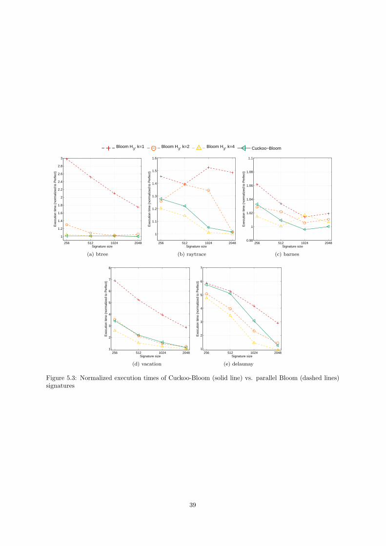
Bloom H3, k=1 Bloom H

3, k=2 Bloom H

3, k=4 Cuckoo−Bloom

256 512 1024 2048

1

1.2

1.4

1.6

1.8

2

2.2

2.4

2.6

2.8

3

Signature size

Exe

cutio

n tim

e (n

orm

aliz

ed to

Per

fect

)

(a) btree

256 512 1024 2048

1

1.1

1.2

1.3

1.4

1.5

1.6

Signature size

Exe

cutio

n tim

e (n

orm

aliz

ed to

Per

fect

)

(b) raytrace

256 512 1024 20480.98

1

1.02

1.04

1.06

1.08

1.1

Signature sizeE

xecu

tion

time

(nor

mal

ized

to P

erfe

ct)

(c) barnes

256 512 1024 20481

2

3

4

5

6

7

8

Signature size

Exe

cutio

n tim

e (n

orm

aliz

ed to

Per

fect

)

(d) vacation

256 512 1024 20481

2

3

4

5

6

7

Signature size

Exe

cutio

n tim

e (n

orm

aliz

ed to

Per

fect

)

(e) delaunay

Figure 5.3: Normalized execution times of Cuckoo-Bloom (solid line) vs. parallel Bloom (dashed lines)signatures

39

Chapter 6

Two adaptive and simple signature

schemes

In this chapter, we describe, analyze, and evaluate two signature schemes that adapt to the size of a

transaction’s read and write-sets. The first one, Hash-Bloom signatures, tries to seek a middle ground

between the accurate hash-table-based representation of Cuckoo-Bloom signatures and the simplicity

of Bloom signatures. It supports all the operations that Bloom signatures support (i.e. works well

with intersection and union), as well as one-cycle insertions and tests. The second one, adaptive Bloom

signatures, uses parallel Bloom signatures, augments each core with read and write-set size predictors,

and adapts the number of hash functions of the signature to the predicted size.

6.1 Hash-Bloom signatures

In the previous chapter, we saw how storing hash values can be used to provide an accurate representation

of small read and write sets, while maintaining a reasonable probability of false positives at high loads.

Cuckoo hashing was helpful in maintaining the structure without Bloom filters until the occupation was

really high, but increased the overall complexity and did not support set union or intersection easily.

With Hash-Bloom signatures, we give up the option of evicting and reinserting elements on a conflict,

and instead, transform the hash table into a Bloom filter gradually.

6.1.1 Design

The basic structure of the Hash-Bloom signature is shown in Figure 6.1a. The table has r rows, each

of which has c bits. Both r and c are a power of two. Additionally, each row features a small register,

which contains the format of the row. The structure uses two hash functions, h1, of log2(r) bits, which

40

is used to index the rows, and h2, of c − 1 bits, used for each row.

h 1

h 2

Address

H 1

H 2

1 0 1 1 1 0 0 1

0 1 1 1 0 1 1 1

0 0 0 0 0 0 0 0

1 1 0 0 0 1 0 0

1 1 0 1 0 1 1 1

0 1 0 1 1 1 0 1

0 0 0 0 0 0 0 0

1 1 0 0 0 1 0 1

3

1

0

2

1

0

0

2

row format

hash bits use bits

(a) Design

h 1

h 2

bitlines

wordlines

1 -ported SRAM

of r·c bits Address

Reduction / Test logic


Figure 6.1: Hash-Bloom Signatures

The structure is cleared by setting the format registers and the last bit of each row to 0. To perform

an insertion, the hash functions are applied to the address, yielding the hash values H1 and H2. H1

determines the row that the element will be in. If the row is empty, we store the c − 1 bits of H2 in the

row, and mark the last bit, the used bit, as 1. To allow the representation of an unbounded number of

elements, each row may support a variable number of entries: one entry of c bits, two of c/2 bits, and

so on, up to c entries of one bit each. In each entry, all the bits but the last store part of the hash value

H2, and the last bit is the used bit. Each inserted element may only map to one entry; this entry is

determined by the first hash bits of H2. If, on an insertion, the entry to fill is already occupied, we check

if the stored bits of H2 match. If they don’t, we have to perform a reduction: we double the number

of entries in the row, remap the current elements in the row, and try to insert the element again. If we

can’t, we perform successive reductions until we are able to1. Note how, in the extreme (c entries of

one bit each), there is no hash information stored, as each entry consists of just the valid bit, and the

insertion cannot fail. In effect, in this case, the row is working like a Bloom filter.

1 0 1 1 1 0 0 1

0 1 1 1 0 1 1 1

0 0 0 0 0 0 0 0

1 1 0 0 0 1 0 0

1 1 0 1 0 1 1 1

0 1 0 1 1 1 0 1

0 0 0 0 0 0 0 0

1 1 0 0 0 1 0 1

3

1

0

2

1

0

0

2

row format

Insert (6,44)

1 0 1 1 1 0 0 1

0 1 1 1 0 1 1 1

0 0 0 0 0 0 0 0

1 1 0 0 0 1 0 0

1 1 0 1 0 1 1 1

0 1 0 1 1 1 0 1

0 1 0 1 1 0 0 1

1 1 0 0 0 1 0 1

3

1

0

2

1

0

0

2

row format

Insert (6,107)

1 0 1 1 1 0 0 1

0 1 1 1 0 1 1 1

0 0 0 0 0 0 0 0

1 1 0 0 0 1 0 0

1 1 0 1 0 1 1 1

0 1 0 1 1 1 0 1

1 1 0 1 1 0 1 1

1 1 0 0 0 1 0 1

3

1

0

2

1

0 ��1

2

row format

Insert (6,19)

1 0 1 1 1 0 0 1

0 1 1 1 0 1 1 1

0 0 0 0 0 0 0 0

1 1 0 0 0 1 0 0

1 1 0 1 0 1 1 1

0 1 0 1 1 1 0 1

1 1 0 0 0 0 0 1

1 1 0 0 0 1 0 1

3

1

0

2

1

0 �2

2

row format

Figure 6.2: Insertion process in a Hash-Bloom signature

The above procedure is best illustrated with an example. Consider, that we have the structure of

Figure 6.1a (8 rows, 8 bits per row). The hash functions h1 and h2 have 3 and 7 bits, respectively. The

example is illustrated in Figure 6.2. Suppose that we begin inserting an element of hash values (6,44).

To do it, we examine the first row, see that it is empty, and place the entry there. Now, to insert an

element with hash values (6,107) we have to perform a reduction, because the element (6,44) is taking

the complete row. We double the number of entries, and remap (6,44). When remapping, the least

significant bit of the stored hash value determines where to map the entry, and hence, it doesn’t need to

1We call this operation reduction because we reduce the number of bits per entry

41

be saved (it is encoded by position). Since 4410 = 01011002, the least significant bit of H2 is 0, and so

the element has to be stored into the first entry. Therefore, the three most significant bits are discarded,

and the value 1102 (bits 3 to 1 of 4410) is stored in the first entry. We now try to reinsert the element.

Since 10710 = 11010112, the least significant bit of H2 is 1, and the element maps into the second entry,

where the bits 1012 are stored. Now both elements are represented in the signature. If we now want to

insert (6,19) (1910 = 00100112), we need an extra reduction: what used to be (6,44) is mapped to the

first entry, with hash value 12; what used to be (6,107) is mapped into the fourth entry, with hash value

02. Since the two least significant bits of 1910 are 112, (6,19) also maps to the fourth entry. However,

the third least significant bit of 19 is 02, so no more reductions are needed: both (6,107) and (6,19)

are represented in the fourth entry now. In short, as successive reductions happen, the most significant

bits of the hash values stored in each entry are trimmed, and the least significant bits are encoded by

position. A signature in which only a few elements are inserted will usually keep many rows with few

entries, and so will represent each inserted element more accurately. Table 6.1 shows the number of hash

bits kept for each entry in a 32x32 filter, depending on the format of the row the element is hashed in.

Format 0 1 2 3 4 5Bits per entry 32 16 8 4 2 1

Hash bits kept, due to row 5 5 5 5 5 5Hash bits kept, by position of entry 0 1 2 3 4 5

Hash bits kept, stored in entry 31 15 7 3 1 0

Hash bits kept, total 36 21 14 11 10 10

Table 6.1: Number of hash bits kept per entry in a 32× 32 Hash-Bloom signature, depending on the rowformat

To test for membership, we compute the hash values H1 and H2, retrieve the row indexed by H1,

and, using the format register, determine the number of entries it contains. Then, the least significant

bits of H2 are used to determine the entry the element is in. If the entry is used and the corresponding

portion of H2 matches with the hash bits stored at the entry, a positive is reported. In any other case,

the element is not represented in the filter.

Additionally, the intersection and union operations of two signatures can be performed in a relatively

short time. The simplest way is to reduce each row of both signatures to a Bloom filter, then perform

the intersection or union operations as it is done in Bloom signatures. Performing an intersection of

these structures without reducing them to Bloom signatures is also easy. The intersection is done row

by row. The first step is to reduce the row with the least number of entries to the number of entries that

the other row has. Then, each pair of entries is compared. If both entries are used and have the same

hash bits, the entry is kept in the intersection; otherwise, it is cleared. Finally, performing an union of

two signatures is more difficult without resorting to Bloom filters, but can be done row by row, and not

element by element, as happened with Cuckoo-Bloom signatures.

42

6.1.2 Analysis

Although this structure is simpler than a Cuckoo-Bloom signature, obtaining a closed-form formula for

the probability of false positives is still complex. Therefore, we perform Monte Carlo analysis to evaluate

the theoretical performance of these signatures. Figure 6.3 shows the probability of false positives for

two signatures of 1Kbit: one with 128 rows and 8 bits/row, and other with 256 rows and 4 bits/row.

0 200 400 600 800 10000

0.1

0.2

0.3

0.4

0.5

0.6

0.7

0.8

0.9

1


Pro

babi

lity

of fa

lse

posi

tives

Bloom and Parallel Hash−Bloom signatures of m=1Kbit

Bloom, k=1Bloom, k=2Bloom, k=4Bloom, k=8Hash−Bloom 4b/rowHash−Bloom 8b/row

0 20 40 60 80 100 120 140 160 1800

0.005

0.01

0.015

0.02

0.025


Pro

babi

lity

of fa

lse

posi

tives


Bloom, k=1Bloom, k=2Bloom, k=4Bloom, k=8Hash−Bloom 4b/rowHash−Bloom 8b/row

Figure 6.3: Probability of false positives for different Hash-Bloom signature configurations

We can see how varying the rows and bits/row gives us a degree of freedom in shaping the probability

of false positives. Signatures with large rows have better behavior for low occupation, because they

retain many hash bits of the inserted elements. Signatures with smaller rows (such as the 256x4 one)

perform worse for low occupations, but do better than a single-hash function Bloom signature even for

quite high occupations. Finally, we can see how the 128x8 signature performs almost as well as a 2-hash

function Bloom signature for small address sets, and as well as a 1-hash function Bloom signature for

large address sets.


Hash-Bloom signatures can be implemented with a single-ported, word-readable SRAM, so the hardware

cost is expected to be similar to that of a Bloom signature of the same size. Figure 6.1b shows a canonical

implementation. The main differences are the higher number of hash bits required, which requires

larger hash functions, and the control logic, which will be more complex. Although in Section 6.1.1 the

reduction process is described in a sequential way (performing successive reductions until the inserted

element fits), the actual hardware implementation can detect how many steps are necessary and do them

at once, enabling one-cycle insertions and tests. This contrasts with the Cuckoo-Bloom signature, where

additions could take a significant number of iterations.

An important factor to take into account is that the space overhead of the flip-flops that maintain the

43

state of each row can impact the total amount of state significatively, especially for signatures with small

rows. For example, in signatures with 4bits/row, each row can have one, two or four entries, needing

two bits to code the format, which results in a 50% overhead (2 extra bits for each 4 bits). However,

a small optimization can save us a lot of space: in general, in these structures, having entries of two

bits does not yield any advantage over 1-bit entries, because the hash bit that we hold in 2-bit entries

is encoded by position when we switch to 1-bit entries (see Table 6.1 for a concrete example). Hence,

we can reduce from 4 bits/entry to 1 bit/entry directly, and remove one state. For 4 bits/row, we just

need an additional bit, and so the overhead is reduced to 25%. Table 6.2 lists the space overheads for

different row lengths.

Bits per row 1 2 4 8 16 32 64Number of formats 1 1 2 3 4 5 6Extra bits per row 0 0 1 2 2 3 3

Space overhead 0% 0% 25% 25% 12.5% 9.37% 4.69%

Table 6.2: Space overhead due to format registers in a Hash-Bloom signature

6.2 Parallel Hash-Bloom Signatures

To reap the benefits of accurate representation of small address sets that Bloom signatures with many

hash functions have, while at the same time we mitigate their poor behavior for large address sets, we

can use multiple Hash-Bloom signatures in parallel. We call this a parallel Hash-Bloom signature.

6.2.1 Design

Figure 6.4a shows the design of a parallel Hash-Bloom signature. As with a parallel Bloom signature, to

insert an element, we insert it in all the signatures, and when testing for membership the result is only

positive if the element is represented in all the signatures.

h 1 h 2

Address

1 0 1 1 1 0 0 1

0 1 1 1 0 1 1 1

0 0 0 0 0 0 0 0

1 1 0 0 0 1 0 0

1 1 0 1 0 1 1 1

0 1 0 1 1 1 0 1

0 0 0 0 0 0 0 0

1 1 0 0 0 1 0 1

3

1

0

2

1

0

0

2

row format

h 3 h 4

1 1 1 0 1 1 0 1

0 1 1 1 0 1 1 1

0 1 0 0 1 1 0 0

1 1 0 1 0 0 1 1

1 1 0 1 0 1 1 1

0 1 0 0 1 1 0 1

0 1 0 1 0 0 0 1

1 1 0 0 1 1 0 0

0

1

2

2

1

3

0

2

row format

h 2k -1 h 2k

0 0 0 0 0 0 0 0

0 1 1 1 0 1 1 1

1 1 0 1 0 0 0 0

0 0 0 0 0 0 0 0

0 0 1 1 0 1 1 1

1 1 0 1 1 1 0 1

0 0 0 0 0 0 0 0

0 1 0 1 0 1 0 1

0

3

1

0

2

1

2

0

row format

(a) Design

h 1

h 2

single-ported SRAM

of r·c bits

Address


h 3

h 4

single-ported SRAM

of r·c bits


h 2k -1

h 2k

single-ported SRAM

of r·c bits


...


Figure 6.4: Parallel Hash-Bloom signatures

6.2.2 Analysis

Figure 6.5 shows the probability of false positives for several signature configurations.

44

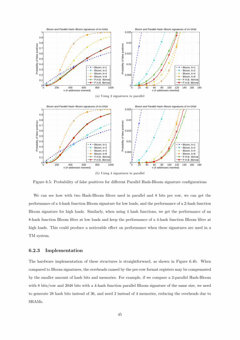
0 200 400 600 800 10000

0.1

0.2

0.3

0.4

0.5

0.6

0.7

0.8

0.9

1


Pro

babi

lity

of fa

lse

posi

tives


Bloom, k=1Bloom, k=2Bloom, k=4Bloom, k=8P.H.B. 4b/rowP.H.B. 8b/row

0 20 40 60 80 100 120 140 160 1800

0.005

0.01

0.015

0.02

0.025


Pro

babi

lity

of fa

lse

posi

tives



(a) Using 2 signatures in parallel

0 200 400 600 800 10000

0.1

0.2

0.3

0.4

0.5

0.6

0.7

0.8

0.9

1


Pro

babi

lity

of fa

lse

posi

tives



0 20 40 60 80 100 120 140 160 1800

0.005

0.01

0.015

0.02

0.025


Pro

babi

lity

of fa

lse

posi

tives



(b) Using 4 signatures in parallel

Figure 6.5: Probability of false positives for different Parallel Hash-Bloom signature configurations

We can see how with two Hash-Bloom filters used in parallel and 8 bits per row, we can get the

performance of a 4-hash function Bloom signature for low loads, and the performance of a 2-hash function

Bloom signature for high loads. Similarly, when using 4 hash functions, we get the performance of an

8-hash function Bloom filter at low loads and keep the performance of a 4-hash function Bloom filter at

high loads. This could produce a noticeable effect on performance when these signatures are used in a

TM system.


The hardware implementation of these structures is straightforward, as shown in Figure 6.4b. When

compared to Bloom signatures, the overheads caused by the per-row format registers may be compensated

by the smaller amount of hash bits and memories. For example, if we compare a 2-parallel Hash-Bloom

with 8 bits/row and 2048 bits with a 4-hash function parallel Bloom signature of the same size, we need

to generate 28 hash bits instead of 36, and need 2 instead of 4 memories, reducing the overheads due to

SRAMs.

45

6.3 Adaptive Bloom signatures

Adaptive Bloom signatures use normal Bloom signatures, but change their amount of hash functions

dynamically in order to adapt to the read and write set sizes of a transactions. Since these sizes are not

known beforehand, we augment each core with simple read and write set size predictors, and infer the

best number of hash functions from the predicted sizes.

6.3.1 Design

The design of the filters is depicted in Figure 6.6a. It consists of a parallel Bloom filter, with a hash

function selection logic, which uses the input from the size predictors to adapt the number of hash

functions.

Address

h 1 h 2 h k ...

0 1 .... 0 1 0 .... 0 0 0 .... 0 ...

h s

Hash function selection logic

PC RS size WS size

0x12f74 25 7

0x13410 138 2

0x104d8 4 1

- - -

Update logic

Prediction table

1 1 0

(a) Design

h 1 h 2 h k ...

Address

...

k single-ported SRAMs of m/ k bits

HF selection (encoder)

write enable signals

h s

Set size counter

Prediction table

Update Logic

EWMA


Figure 6.6: Adaptive Bloom Signatures

Predictors: The size predictor has two main components: the prediction table and the prediction

update logic. The prediction table (see Figure 6.6a) stores the current size predictions. Each entry in

the table stores the predicted read and write set sizes for a certain type of transaction. This type is

determined by the value of the program counter when the transaction begins, so that multiple instances

of the same transactional code use the same prediction. The table has a limited number of entries, and

follows a LRU eviction policy: if we begin a transaction whose size prediction is not in the predictor

table, we evict the least recently used entry. Typically, a small number of entries will be enough (e.g. 4

entries produce no evictions in our simulations).

The prediction update logic keeps track of the current transaction’s read and write set sizes by incre-

menting a counter each time an element is inserted into the signatures, and updates the size predictions

when a transaction commits. The new predicted value is calculated using an exponential weighted moving

average (EWMA). In general, this uses the formula:

NewPrediction = α · NewV alue + (1 − α) · OldPrediction, 0 ≤ α ≤ 1

Note that the α parameter (called smoothing factor) determines how much we take the new value into

account in the prediction. An α close to 0 causes a smooth but slowly changing prediction, while an α

46

close to 1 causes the prediction to change swiftly but may be less stable if the values change a lot. In our

case, we would like to be somewhat pessimistic with set size prediction, i.e. it is preferred to overestimate

the size than to underestimate it, to avoid the saturation of the signature if we select a high number of

hash functions and the set size is larger than expected. To achieve this, we use two different values of α

to make the prediction:

• If SizeAtCommit > PredictedSize, NewPredictedSize = 34SizeAtCommit + 1

4PredictedSize.

• If SizeAtCommit < PredictedSize, NewPredictedSize = 14SizeAtCommit + 3

4PredictedSize.

Finally, note that by using the values 1/4 (a power of 2) and 3/4 in the calculations, we enable a

simple hardware implementation of the update logic.

Hash function selection: The hash function selection logic also has two components: First, the

number of hash functions to be used, kp, has to be deduced from the predicted set size. Since this

involves some amount of probabilistic reasoning, the procedure will be explained in the analysis section.

Second, we have to select the actual hash functions to use, given kp. If we used a k hash function true

Bloom signature, doing this would be trivial: we could just use the first kp hash functions. However, this

is not possible in a k hash function parallel Bloom signature, since using a fixed set of hash functions

leaves part of the filter unused. To cope with this, we will use an additional small hash function hs,

which will be applied to each incoming address, generating a hash value 0 ≤ Hs < kp, and will use the

hash functions (and memories) with index Hs, (Hs + 1) mod k, ..., (Hs + kp − 1) mod k. For example,

if we have k = 8 hash functions, and kp = 4, when Hs = 3 we will use hash functions 3,4,5, and 6, and

when Hs = 6 we will use hash functions 6,7,0, and 1.

6.3.2 Analysis

An adaptive Bloom signature will work just as a Bloom signature in terms of probability of false positives

for a certain transaction, but will change the number of hash functions used over time. We now focus

on how to select the best number of hash functions. Recall from Section 4.3 that the best number of

hash functions to be used was kopt = mn ln(2). Although m (the size of the filter) is fixed and the ln(2)

term could be approximated by other easier to compute constant (such as 3/4), the calculation is still

not trivial to implement in hardware. An easier alternative is to hardcode the ranges in which each

number of hash functions is optimal, and use a set of comparators. Table 6.3 lists these ranges for a

1024-bit Bloom signature. However, this still requires a high amount of comparators to be implemented.

If we want to use a really simple selection logic, we may choose to use a smaller subset of hash function

numbers. For example, suppose that we want to use either 1, 2, 4, or 8 hash functions. Figure 6.7 has the

47

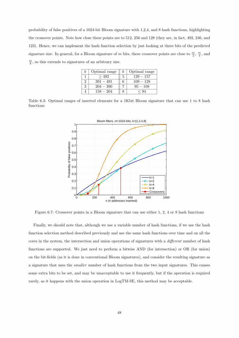
probability of false positives of a 1024-bit Bloom signature with 1,2,4, and 8 hash functions, highlighting

the crossover points. Note how close these points are to 512, 256 and 128 (they are, in fact, 492, 246, and

123). Hence, we can implement the hash function selection by just looking at three bits of the predicted

signature size. In general, for a Bloom signature of m bits, these crossover points are close to m2 , m

4 , and

m8 , so this extends to signatures of an arbitrary size.

k Optimal range k Optimal range1 ≥ 492 5 129 − 1572 391 − 491 6 109 − 1283 204 − 390 7 95 − 1084 158 − 204 8 ≤ 94

Table 6.3: Optimal ranges of inserted elements for a 1Kbit Bloom signature that can use 1 to 8 hashfunctions

0 200 400 600 800 10000

0.1

0.2

0.3

0.4

0.5

0.6

0.7

0.8

0.9

1


Pro

babi

lity

of fa

lse

posi

tives


k=1k=2k=4k=8Crossovers

Figure 6.7: Crossover points in a Bloom signature that can use either 1, 2, 4 or 8 hash functions

Finally, we should note that, although we use a variable number of hash functions, if we use the hash

function selection method described previously and use the same hash functions over time and on all the

cores in the system, the intersection and union operations of signatures with a different number of hash

functions are supported. We just need to perform a bitwise AND (for intersection) or OR (for union)

on the bit-fields (as it is done in conventional Bloom signatures), and consider the resulting signature as

a signature that uses the smaller number of hash functions from the two input signatures. This causes

some extra bits to be set, and may be unacceptable to use it frequently, but if the operation is required

rarely, as it happens with the union operation in LogTM-SE, this method may be acceptable.

48


Implementing an adaptive Bloom signature requires, apart from the Bloom signature, to implement the

size predictors and the hash function selection logic. An implementation can be seen in Figure 6.6b.

Note that, since the output of the predictors is to be used in selecting the number of hash functions,

the predicted sizes need just a small number of bits. For example, for a 1Kbit signature, 10 bits per

prediction would be more than enough. Also, if we use a limited number of hash functions and high

precision is not a concern, we can discard the least significant bits of the prediction as well. To predict

whether to use 1, 2, 4, or 8 hash functions as described in the previous subsection, just 3 or 4 bits of

the predicted size need to be stored (i.e. we would discard the 6 or 7 least significant bits of the set size

counters). In the end, the additional hardware requirements are:

• A small set of flip-flops or a small SRAM to hold the prediction table. If space is a concern, the

program counter needn’t be stored completely: we could hash it and store its hash value, as it is

often done in other prediction schemes (such as branch predictors).

• Two saturating counters to track the transaction’s read and write set sizes.

• Some simple logic to update the size predictions (mainly, about two multiplexors and small adders).

Note that, since updates are seldom done, the circuit can take multiple cycles to operate and/or

could be used to update the predictions of both the read and write sets.

• A combinational circuit to select kp, which can be made very simple, as explained in the previous

subsection.

• An additional hash function hs, which is small (e.g. 3 bits for 8 hash functions), and logic to select

the appropriate subset of hash functions to be used in each operation.

As a conclusion, the area requirements of the predictors and hash selection logic can be made small

with respect to the area taken up by signatures, especially for signatures of a few kilobits.


We now present a performance evaluation of both Hash-Bloom signatures and adaptive Bloom signatures,

comparing them with parallel Bloom signatures of similar characteristics.

6.4.1 Hash-Bloom and Parallel Hash-Bloom signatures

By their structure, Hash-Bloom signatures should always do better than Bloom signatues of the same

configuration and size. The performance of different signature configurations for our set of benchmarks

can be seen in Figure 6.8. In all the Hash-Bloom signatures, a value of 8 bits/row is used.

49


3, k=2 Bloom H

3, k=4 HashBloom H

3, k=1 HashBloom H

3, k=2 HashBloom H

3, k=4

256 512 1024 2048

1

1.2

1.4

1.6

1.8

2

2.2

2.4

2.6

2.8

3

Signature size

Exe

cutio

n tim

e (n

orm

aliz

ed to

Per

fect

)

(a) btree

256 512 1024 2048

1

1.1

1.2

1.3

1.4

1.5

1.6

Signature sizeE

xecu

tion

time

(nor

mal

ized

to P

erfe

ct)

(b) raytrace

256 512 1024 20480.98

1

1.02

1.04

1.06

1.08

1.1

Signature size

Exe

cutio

n tim

e (n

orm

aliz

ed to

Per

fect

)

(c) barnes

256 512 1024 20481

2

3

4

5

6

7

8

Signature size

Exe

cutio

n tim

e (n

orm

aliz

ed to

Per

fect

)

(d) vacation

256 512 1024 20481

2

3

4

5

6

7

Signature size

Exe

cutio

n tim

e (n

orm

aliz

ed to

Per

fect

)

(e) delaunay

Figure 6.8: Normalized execution times of Hash-Bloom (solid lines) vs. parallel Bloom (dashed lines)signatures

As we can see, Hash-Bloom and parallel Hash-Bloom signatures do better than their Bloom coun-

terparts across all the benchmarks (with the notable exception of raytrace, which can be attributed to

the different set of hash functions used). The difference is most remarkable when comparing single hash

function Bloom signatures versus single Hash-Bloom signatures. However, the difference decreases when

comparing with Bloom signatures of multiple hash functions, especially of k = 4. Also, we can see that

there is a high correlation with theory: a single Hash-Bloom signature does almost as well as 2-hash

function Parallel Bloom, a 2-parallel Hash-Bloom comparably to a 4 hash function parallel Bloom, and

a 4 hash function parallel Hash-Bloom surpasses both Bloom filters of 4 and 8 hash functions.

6.4.2 Adaptive Bloom signatures

Figure 6.9 shows the performance of adaptive Bloom signatures versus parallel Bloom signatures, using

fixed H3 hash functions. The adaptive Bloom filter uses 1,2,4 or 8 hash functions, following the inexpen-

sive mechanism described in Section 6.3.1 to select the appropriate number. The prediction table has 4

entries.

50


3, k=2 Bloom H

3, k=4 Bloom H

3, k=8 Adaptive Bloom H

3, k=1−2−4−8

256 512 1024 2048

1

1.2

1.4

1.6

1.8

2

2.2

2.4

2.6

2.8

3

Signature size

Exe

cutio

n tim

e (n

orm

aliz

ed to

Per

fect

)

(a) btree

256 512 1024 2048

1

1.1

1.2

1.3

1.4

1.5

1.6

Signature sizeE

xecu

tion

time

(nor

mal

ized

to P

erfe

ct)

(b) raytrace

256 512 1024 20480.98

1

1.02

1.04

1.06

1.08

1.1

Signature size

Exe

cutio

n tim

e (n

orm

aliz

ed to

Per

fect

)

(c) barnes

256 512 1024 20481

2

3

4

5

6

7

8

Signature size

Exe

cutio

n tim

e (n

orm

aliz

ed to

Per

fect

)

(d) vacation

256 512 1024 20481

2

3

4

5

6

7

Signature size

Exe

cutio

n tim

e (n

orm

aliz

ed to

Per

fect

)

(e) delaunay

Figure 6.9: Normalized execution times of adaptive Bloom (solid lines) vs. parallel Bloom (dashed lines)signatures

We can see how the signature performs in the range of a 4 hash function Bloom signature and an

8-hash function Bloom signature across all the sizes and benchmarks. Table 6.4 lists the percentage of

time that 1, 2, 4 and 8 hash functions were used for the different benchmarks for a 512-bit adaptive

Bloom signature, as well as the predicted and actual mean set sizes, for the largest type of transaction

in each benchmark (not for all the transactions in the workload). We can see that the simple prediction

mechanism works as expected, and slightly overestimates the size. Also, the number of hash functions

adapts accordingly: in benchmarks with small read/write sets, 8 hash functions are always used. However,

raytrace and vacation, which have larger read sets, the hash value usage distribution adapts accordingly.

Read set Write setBenchmark k =1/2/4/8 (%) Size Prediction k =1/2/4/8 (%) Size Prediction

btree 0 / 0 / 0 / 100 13 13.25 0 / 0 / 0 / 100 1.97 2.93raytrace 39 / 20 / 15 / 26 193.8 210.9 0 / 0 / 0 / 100 2.11 1.07barnes 0 / 0 / 0 / 100 5.58 7.11 0 / 0 / 0 / 100 4.41 5.17

vacation 0 / 5 / 88 / 7 80.9 96.4 0 / 0 / 0 / 100 12.6 13.7

Table 6.4: Hash function usage distribution on the largest transaction type for a 512-bit adaptive Bloomsignature

51

As a conclusion, adaptive Bloom signatures may be effective to avoid the saturation of the signatures if

we intend to use a high number of hash functions. While this need does not show in our benchmarks, it is

possible that future applications with a more widely varying behavior may experience a more significant

performance boost when using this technique.

52

Chapter 7

The interaction of signatures with

system parameters

Now that the different signature schemes have been discussed, it is time to see how signatures interact

with other parameters in the system. Specifically, we will see how signatures become critical as the

number of cores in the system increases, how much can we improve performance by using a directory to

filter out signature tests, and whether the different conflict resolution protocols designed for LogTM-SE

and presented in Chapter 2 help with false conflicts or make them worse. Along this chapter, we will use

parallel Bloom signatures with H3 hash functions, under different configurations.

7.1 Effect of the number of cores

Figure 7.1 shows the normalized execution time for the different workloads as a function of the number of

cores in the system (in the x-axis), both when a broadcast protocol (solid lines) and a directory protocol

(dashed lines) are used, for 256-bit parallel Bloom signatures with 2 and 4 fixed H3 hash functions. As we

vary the number of cores in the CMP system, the rest of parameters (cache sizes, interconnection fabric

and delays, number of memory controllers, etc.) stay the same. Focusing on the broadcast protocol, we

can see that the impact of having weak signatures increases dramatically with the number of cores. For

example, in btree and raytrace, 256-bit 2 hash functions signatures introduce no performance degradation

at all, while for 32 processors they cause degradations of 38% and 24%, respectively. In vacation, the

same signature configuration has a 50% performance penalty with 8 processors, and a 350% penalty with

32 cores.

53

Bloom H3, k=2, Broadcast Bloom H

3, k=4, Broadcast Bloom H

3, k=2, Directory Bloom H

3, k=4, Directory

8 16 320.95

1

1.05

1.1

1.15

1.2

1.25

1.3

1.35

1.4

Number of processors

Exe

cutio

n tim

e (n

orm

aliz

ed to

Per

fect

)

(a) btree

8 16 320.95

1

1.05

1.1

1.15

1.2

1.25

1.3


Exe

cutio

n tim

e (n

orm

aliz

ed to

Per

fect

)

(b) raytrace

8 16 320.98

1

1.02

1.04

1.06

1.08

1.1


Exe

cutio

n tim

e (n

orm

aliz

ed to

Per

fect

)

(c) barnes

8 16 32

1

1.5

2

2.5

3

3.5

4


Exe

cutio

n tim

e (n

orm

aliz

ed to

Per

fect

)

(d) vacation

Figure 7.1: Normalized execution times of 256-bit parallel Bloom signatures for 8 to 32 processors, witha broadcast protocol (solid lines) and a directory (dashed lines)

7.2 Effect of using the directory as a filter

By examining Figure 7.1 we can also appreciate the benefits of using the directory protocol proposed in

LogTM-SE and described in section 2.2 instead of the broadcast one. We can see how the directory is

typically quite effective in reducing false positives (as fewer tests are performed), so small signatures are

usually sufficient even for a large number of cores. For example, for 32 cores and 256-bit signatures with

2 hash functions, the performance penalties in btree, raytrace, and vacation are now of 2%, 18%, and

240% (respectively), instead of the 38%, 24% and 350% obtained with the broadcast protocol. However,

we can also see that, even with a directory, the performance degradation increases when we have more

cores. Therefore, using a directory to reduce the number of false positives scales better with the number

of cores than broadcasting, but the signature size still needs to increase in order to keep false positives

rare.

7.3 Effect of the conflict resolution protocols

Finally, we study how the impact of signatures on performance varies as we change the conflict resolution

protocol. Recall that, in the previous experiments, we have been using the basic conflict resolution

protocol with write-set prediction. The other alternatives were explained in Section 2.3. We will study

the differences between three choices:

1. Basic conflict resolution protocol, without write-set prediction (Base/NoPred)

2. Basic conflict resolution protocol, with write-set prediction (Base/Pred)

3. Hybrid conflict resolution protocol, with write-set prediction (Hybrid/Pred)

54

Figure 7.2 shows the normalized execution times in a 32-core system using a broadcast protocol, with

Bloom signatures of 2 fixed H3 hash functions and sizes from 256 to 2048 bits, using the three different

conflict resolution protocols. This time, the execution times are not normalized, to take into account

the real benefit of each conflict resolution protocol. Instead, we show the execution time with perfect

signatures at the right of each graph as a reference.

Base/NoPred Base/Pred Hybrid/Pred

256 512 1024 2048 Perfect

5

5.5

6

6.5

7

7.5x 10

6

Signature size/type

Exe

cutio

n tim

e

(a) btree

256 512 1024 2048 Perfect1.8

1.9

2

2.1

2.2

2.3

2.4

2.5

2.6

2.7

2.8

2.9x 10

7

Signature size/type

Exe

cutio

n tim

e

(b) raytrace

256 512 1024 2048 Perfect1.13

1.135

1.14

1.145

1.15

1.155

1.16

1.165

1.17

1.175

1.18x 10

7

Signature size/type

Exe

cutio

n tim

e

(c) barnes

256 512 1024 2048 Perfect

1

1.5

2

2.5

3

x 107

Signature size/type

Exe

cutio

n tim

e

(d) vacation

256 512 1024 2048 Perfect

1

1.5

2

2.5

3

3.5

4

4.5

5

x 107

Signature size/type

Exe

cutio

n tim

e

(e) delaunay

Figure 7.2: Execution times of 256-bit 2-hash function parallel Bloom signatures with different conflictresolution protocols

As we can see, having write-set prediction is fairly orthogonal to the effect of signatures, as the

separation between the lines of the schemes with and without prediction remains approximately constant

as we change the signature size. However, this does not apply when using the hybrid conflict resolution

protocol: in btree and raytrace the execution time is affected less when reducing the signature size with

the hybrid conflict resolution policy. This might seem counterintuitive, because the protocol causes more

false aborts, and these waste work and take some time to complete. However, the situation that this

protocol tries to avoid (having an older writer nacked by younger readers, as we saw in Section 2.3)

becomes much more important when false positives happen, degrading performance much more, so

preventing it outweighs the penalty of having more false aborts. In vacation and delaunay, which do not

55

exhibit this pathology, this protocol performs on par with the others.

We can draw two conclusions from these results. First, the choice of the conflict resolution protocol

should not be significantly influenced by a the choice of signatures, as the best performing protocol

with perfect signatures is still the best across all the tested signature sizes for each of our benchmarks.

Second, we see that the hybrid conflict resolution protocol with write-set prediction outperforms the other

two over all the benchmarks except vacation (where not having write-set prediction actually helps by

increasing the number of aborts), so, overall, it seems the protocol of choice regardless of the signatures

used (we extend the observations of Bobba et al. [6], who reach this conclusion for a system with perfect

signatures).

56

Chapter 8

Conclusions

Signature-based conflict detection is a promising approach in TM systems, as it enables transactions

unbounded in size in a hardware-efficient manner, at the expense of a typically small performance hit if

good signatures are used. Multiple signature-based designs have been proposed so far, but the novelty

and complexity of these systems left little room to cover in depth the different approaches to signature

implementation and their implications.

In this study, we have examined the design and implementation of multiple signature schemes. First,

we have studied Bloom signatures in depth, and used the theory behind them to obtain a key result:

that parallel Bloom signatures are much more area-efficient than true Bloom signatures because they

require single-ported memories instead of a multi-ported one. We have shown that this can lead to 8×

area savings when using four hash functions. The performance evaluation of Bloom signatures, the first

to exploit their three design dimensions (size, number of hash functions, and type of hash functions), has

lead to important results:

1. There are alternatives to the commonly used bit-selection hash functions, such as the H3 family of

hash functions, that achieve better performance while being hardware-inexpensive.

2. Signatures that use a high number of good hash functions (about 4) significantly reduce the per-

formance degradation of signatures, if used with high quality hash functions.

3. Introducing some kind of variability over time in the hash functions can be very useful, preventing

repeated signature aliases and leading to a highly robust signature design.

4. The equivalence between true and parallel Bloom signatures holds in practice, provided that good

hash functions are used, even when the conditions assumed in the theoretical analysis are not

strictly met.

57

Additionally, we have designed, described, and evaluated three novel types of signatures. First,

Cuckoo-Bloom signatures, which adapt cuckoo hashing to represent small read or write sets with high

accuracy (an important case), and morph into a Bloom filter as the size of the represented set increases

to achieve good behavior for large sets. Cuckoo-Bloom signatures achieve an insignificant performance

degradation when the represented sets of addresses usually fit in the structure, but degrade less gracefully

than Bloom filters. Second, Hash-Bloom signatures, which combine hashing and Bloom filters in a sim-

pler way than Cuckoo-Bloom signatures, allow to have multiple of them working in parallel, and perform

better than their Bloom signature counterparts. And third, adaptive Bloom signatures, which predict

the read and write set sizes of a transaction and adapt the number of hash functions used by a parallel

Bloom signature accordingly. When classical probabilistic characterization of these new structures was

unfeasible, we used Monte Carlo simulations to analyze them.

Finally, we have studied the interaction of false conflicts caused by signatures and other system

parameters, such as the number of cores and conflict resolution protocols, and have found that: (1)

increasing number of cores places a higher pressure in the signatures of the system, (2) using a directory

protocol effectively mitigates much of this extra pressure, and (3) the kind of signatures used does not

have a significant impact on the conflict resolution protocol of choice, as the protocol that works best

with perfect signatures in each case is also the best for all signature sizes.

Future work

While this study tries to cover the aspects of signature design and implementation comprehensively, some

aspects are still object of future work. First, although the benchmarks used in the evaluation are insightful

and exhibit widely varying behaviors, they are probably not representative of the full spectrum of TM

workloads. Future studies could use a richer set of benchmarks for a more thorough evaluation. Also,

we have used a limited set of hash functions to prove that their quality plays an important role, but we

do not study what is the optimal tradeoff between hash function quality and area efficiency. Regarding

the different implementations, we provide area and complexity estimations for each signature design,

but do not give an in-depth comparison with exact area and delay numbers of actual implementations.

Finally, the performance evaluation is done with LogTM-SE, but signatures can be used in other ways in

alternative TM systems. Although the basic theoretical principles of each signature design remain valid,

quantifying te impact that the different designs have on other TM systems remains an object of future

work as well.

58

Bibliography

[1] A. R. Alameldeen and D. A. Wood. Variability in architectural simulations of multi-threaded work-

loads. In HPCA ’03: Proceedings of the 9th International Symposium on High-Performance Com-

puter Architecture, page 7, Feb. 2003.

[2] C. S. Ananian, K. Asanovic, B. C. Kuszmaul, C. E. Leiserson, and S. Lie. Unbounded transac-

tional memory. In Proceedings of the Eleventh IEEE Symposium on High-Performance Computer

Architecture, Feb. 2005.

[3] W. Baek, C. Cao Minh, M. Trautmann, C. Kozyrakis, and K. Olukotun. The OpenTM transactional

application programming interface. In Proceedings of the 16th International Conference on Parallel

Architectures and Compilation Techniques. Sep 2007.

[4] B. H. Bloom. Space/time trade-offs in hash coding with allowable errors. Commun. ACM, 13(7):422–

426, July 1970.

[5] C. Blundell, J. Devietti, E. C. Lewis, and M. M. K. Martin. Making the fast case common and

the uncommon case simple in unbounded transactional memory. SIGARCH Comput. Archit. News,

35(2):24–34, 2007.

[6] J. Bobba, K. E. Moore, H. Volos, L. Yen, M. D. Hill, M. M. Swift, and D. A. Wood. Performance

pathologies in Hardware Transactional Memory. In Proceedings of the 34th International Symposium

on Computer Architecture, pages 81–91, June 2007.

[7] F. Bonomi, M. Mitzenmacher, R. Panigrahy, S. Singh, and G. Varghese. Bloom filters via d-left

hashing and dynamic bit reassignment. In Allerton’06, 2006.

[8] F. Bonomi, M. Mitzenmacher, R. Panigrahy, S. Singh, and G. Varghese. An improved construction

for counting Bloom filters. In Proceedings of the European Symposium on Algorithms ’06, pages

684–695, 2006.

[9] A. Broder and M. Mitzenmacher. Network applications of Bloom filters: A survey. Internet Math-

ematics, 1(4):485–509, 2004.

59

[10] J. L. Carter and M. N. Wegman. Universal classes of hash functions (extended abstract). In STOC

’77: Proceedings of the ninth annual ACM symposium on Theory of computing, pages 106–112, 1977.

[11] L. Carter, R. Floyd, J. Gill, G. Markowsky, and M. Wegman. Exact and approximate membership

testers. In STOC ’78: Proceedings of the tenth annual ACM symposium on Theory of computing,

pages 59–65, 1978.

[12] L. Ceze, J. Tuck, C. Cascaval, and J. Torrellas. Bulk disambiguation of speculative threads in multi-

processors. In Proceedings of the 33rd Annual International Symposium on Computer Architecture,

June 2006.

[13] L. Ceze, J. Tuck, P. Montesinos, and J. Torrellas. BulkSC: Bulk enforcement of sequential consis-

tency. In Proceedings of the 34th Annual International Symposium on Computer Architecture, June

2007.

[14] B. Chazelle, J. Kilian, R. Rubinfeld, and A. Tal. The Bloomier filter: an efficient data structure

for static support lookup tables. In SODA ’04: Proceedings of the fifteenth annual ACM-SIAM

symposium on Discrete algorithms, pages 30–39, 2004.

[15] S. Cohen and Y. Matias. Spectral Bloom filters. In SIGMOD ’03: Proceedings of the 2003 ACM

SIGMOD international conference on Management of data, pages 241–252, 2003.

[16] P. Damron, A. Fedorova, Y. Lev, V. Luchango, M. Moir, and D. Nussbaum. Hybrid transactional

memory, Oct. 2006.

[17] S. Dharmapurikar, P. Krishnamurthy, T. Sproull, and J. Lockwood. Deep packet inspection using

parallel Bloom filters. IEEE Micro, 24(1):52–61, 2004.

[18] L. Fan, P. Cao, J. Almeida, and A. Z. Broder. Summary cache: a scalable wide-area web cache

sharing protocol. IEEE/ACM Trans. Netw., 8(3):281–293, 2000.

[19] M. Ghosh, E. Ozer, S. Biles, and H.-H. S. Lee. Efficient system-on-chip energy management with

a segmented Bloom filter. In Proceedings of the 19th International Conference on Architecture of

Computing Systems, pages 283–297, March 2006.

[20] L. Hammond, V. Wong, M. Chen, B. D. Carlstrom, J. D. Davis, B. Hertzberg, M. K. Prabhu,

H. Wijaya, C. Kozyrakis, and K. Olukotun. Transactional memory coherence and consistency. In

Proceedings of the 31st Annual International Symposium on Computer Architecture, June 2004.

[21] M. Herlihy, V. Luchangco, M. Moir, and W. Scherer. Software transactional memory for dynamic-

sized data structures. In Proceedings of the 22nd Annual ACM Symposium on Principles of Dis-

tributed Computing (July 2003), pp. 92–101., 2003.

60

[22] M. Herlihy and J. E. B. Moss. Transactional memory: Architectural support for lock-free data struc-

tures. In Proceedings of the Twentieth Annual International Symposium on Computer Architecture,

pages 289–300, May 1993.

[23] P. Kongetira, K. Aingaran, and K. Olukotun. Niagara: A 32-way multithreaded SPARC processor.

IEEE Micro, 25(2):21–29, 2005.

[24] L. Lamport. Time, clocks, and the ordering of events in a distributed system. Commun. ACM,

21(7):558–565, 1978.

[25] J. R. Larus and R. Rajwar. Transactional Memory. Morgan & Claypool Publishers, 2006.

[26] M. Martin, C. Blundell, and E. Lewis. Subtleties of transactional memory atomicity semantics.

IEEE Comput. Archit. Lett., 5(2):17, 2006.

[27] M. M. Martin, D. J. Sorin, B. M. Beckmann, M. R. Marty, M. Xu, A. R. Alameldeen, K. E. Moore,

M. D. Hill, and D. A. Wood. Multifacet’s general execution-driven multiprocessor simulator (GEMS)

toolset. Computer Architecture News, pages 92–99, Sept. 2005.

[28] C. C. Minh, M. Trautmann, J. Chung, A. McDonald, N. Bronson, J. Casper, C. Kozyrakis, and

K. Olukotun. An effective hybrid transactional memory system with strong isolation guarantees. In

Proceedings of the 34th Annual International Symposium on Computer Architecture, June 2007.

[29] M. Mitzenmacher. Compressed Bloom filters. In PODC ’01: Proceedings of the twentieth annual

ACM symposium on Principles of distributed computing, pages 144–150, 2001.

[30] K. E. Moore, J. Bobba, M. J. Moravan, M. D. Hill, and D. A. Wood. LogTM: Log-based transac-

tional memory. In Proceedings of the 12th International Symposium on High-Performance Computer

Architecture, pages 254–265, Feb 2006.

[31] A. Pagh, R. Pagh, and S. S. Rao. An optimal Bloom filter replacement. In SODA ’05: Proceedings

of the sixteenth annual ACM-SIAM symposium on Discrete algorithms, pages 823–829, 2005.

[32] R. Pagh and F. F. Rodler. Cuckoo hashing. In ESA ’01: Proceedings of the 9th Annual European

Symposium on Algorithms, pages 121–133, 2001.

[33] R. Rajwar, M. Herlihy, and K. Lai. Virtualizing transactional memory. In ISCA ’05: Proceedings

of the 32nd Annual International Symposium on Computer Architecture, pages 494–505, 2005.

[34] M. V. Ramakrishna. Practical performance of Bloom filters and parallel free-text searching. Com-

mun. ACM, 32(10):1237–1239, 1989.

61

[35] M. V. Ramakrishna, E. Fu, and E. Bahcekapili. Efficient hardware hashing functions for high

performance computers. IEEE Trans. Comput., 46(12):1378–1381, 1997.

[36] E. Safi, A. Moshovos, and A. Veneris. L-CBF: a low-power, fast counting Bloom filter architecture.

In ISLPED ’06: Proceedings of the 2006 International Symposium on Low Power Electronics and

Design, pages 250–255, 2006.

[37] B. Saha, A.-R. Adl-Tabatabai, and Q. Jacobson. Architectural support for software transactional

memory. In MICRO 39: Proceedings of the 39th Annual IEEE/ACM International Symposium on

Microarchitecture, pages 185–196, 2006.

[38] D. Sanchez, L. Yen, M. D. Hill, and K. Sankaralingam. Implementing Signatures for Transactional

Memory. In MICRO 40: Proceedings of the 40th Annual IEEE/ACM International Symposium on

Microarchitecture, Dec. 2007.

[39] S. Sethumadhavan, R. Desikan, D. Burger, C. R. Moore, and S. W. Keckler. Scalable hardware

memory disambiguation for high-ILP processors. IEEE Micro, 24(6):118–127, 2004.

[40] N. Shavit and D. Touitou. Software transactional memory. In Symposium on Principles of Distributed

Computing, pages 204–213, 1995.

[41] D. Tarjan, S. Thoziyoor, and N. P. Jouppi. CACTI 4.0. Technical Report HPL-2006-86, HP Labs,

2006.

[42] H. Vandierendonck and K. D. Bosschere. XOR-based hash functions. IEEE Trans. Comput.,

54(7):800–812, 2005.

[43] J.-M. Wang, S.-C. Fang, and W.-S. Feng. New efficient designs for XOR and XNOR functions on

the transistor level. IEEE Journal of Solid-State Circuits, 29(7):780–786, July 1994.

[44] S. C. Woo, M. Ohara, E. Torrie, J. P. Singh, and A. Gupta. The SPLASH-2 programs: Characteriza-

tion and methodological considerations. In ISCA ’95: Proceedings of the 22nd Annual International

Symposium on Computer Architecture, pages 24–36, June 1995.

[45] L. Yen, J. Bobba, M. R. Marty, K. E. Moore, H. Volos, M. D. Hill, M. M. Swift, and D. A. Wood.

LogTM-SE: Decoupling hardware transactional memory from caches. In Proceedings of the 13th

International Symposium on High-Performance Computer Architecture, pages 261–272, Feb 2007.

[46] A. Zeichick. One, two, three, four: A sneak peek inside AMD’s forthcoming quad-core processors.

Technical report, AMD, Jan. 2007.

62

Design and Implementation of Signatures for Transactional...

Documents

Transcript of Design and Implementation of Signatures for Transactional...