Design and Implementation of Practical Constraint Logic ...fp/public/elf-papers/michaylov92.pdf ·...
229
Design and Implementation of Practical Constraint Logic Programming Systems Spiro Michaylov August 24, 1992 CMU-CS-92-168 School of Computer Science Carnegie Mellon University 5000 Forbes Avenue Pittsburgh, PA 15213-3891 Submitted in partial fulfillment of the requirements for the degree of Doctor of Philosophy. c 1992 by Spiro Michaylov This research was sponsored partly by IBM through a graduate fellowship and a joint study agree- ment, and partly by the Avionics Laboratory, Wright Research and Development Center, Aeronautical Systems Division (AFSC), U. S. Air Force, Wright-Patterson AFB, OH 45433-6543 under Contract F33615-90-C-1465, ARPA Order No. 7597. The views and conclusions contained in this document are those of the author and should not be interpreted as representing the official policies, either expressed or implied, of the U.S. Government.
Transcript of Design and Implementation of Practical Constraint Logic ...fp/public/elf-papers/michaylov92.pdf ·...

Design and Implementation ofPractical
Constraint Logic Programming Systems
Spiro Michaylov
August 24, 1992
CMU-CS-92-168
School of Computer ScienceCarnegie Mellon University
5000 Forbes AvenuePittsburgh, PA 15213-3891
Submitted in partial fulfillment of the requirementsfor the degree of Doctor of Philosophy.
c©1992 by Spiro Michaylov
This research was sponsored partly by IBM through a graduate fellowship and a joint study agree-ment, and partly by the Avionics Laboratory, Wright Research and Development Center, AeronauticalSystems Division (AFSC), U. S. Air Force, Wright-Patterson AFB, OH 45433-6543 under ContractF33615-90-C-1465, ARPA Order No. 7597.
The views and conclusions contained in this document are those of the author and should not beinterpreted as representing the official policies, either expressed or implied, of the U.S. Government.

Keywords: programming languages, declarative programming, logic program-ming, constraints, programming methodology, efficient implementation

Abstract
The Constraint Logic Programming (CLP) scheme, developed by Jaffar and Lassez,defines a class of rule–based constraint programming languages. These generalize tra-ditional logic programming languages (like Prolog) by replacing the basic operationalstep, unification, with constraint solving. While CLP languages have a tremendousadvantage in terms of expressive power, they must be shown to be amenable to prac-tical implementations. This thesis describes a systematic approach to the design andimplementation of practical CLP systems. The approach is evaluated with respect totwo major objectives. First, the Prolog subset of the languages must be executed withessentially the efficiency of an equivalent Prolog system. Second, the cost of constraintsolving must be commensurate with the complexity of the constraints arising.
The language CLP(R), whose domain is uninterpreted functors over real numbers,is the central case study. First, the design of CLP(R) is discussed in relation to pro-gramming methodology. The discussion of implementation begins with an interpreterthat achieves the efficiency of equivalent Prolog interpreters, and meets many of thebasic efficiency requirements for constraint solving. Many of the principles applied inthe interpreter are then used to develop an abstract machine for CLP(R), leading to acompiler-based system achieving performance comparable to modern Prolog compilers.Furthermore, it is shown how this technology can be extended so that the efficiencyof CLP(R) approaches that of imperative programming languages. Finally, to demon-strate the wider applicability of the techniques developed, it is shown how they canbe used to design and implement a version of Elf, a language with equality constraintsover λ-expressions with dependent types.
iii

Contents
I Background 1
1 Introduction 2
2 Constraints and Logic Programming 72.1 Logic Programming and Prolog . . . . . . . . . . . . . . . . . . . . . . . 7
2.1.1 The Prolog Operational Model . . . . . . . . . . . . . . . . . . . 72.1.2 Implementation Techniques . . . . . . . . . . . . . . . . . . . . . 112.1.3 Programming Methodology and Practical Experience . . . . . . . 12
2.2 Constraints and Constraint Programming . . . . . . . . . . . . . . . . . 122.2.1 Constraint Solving . . . . . . . . . . . . . . . . . . . . . . . . . . 132.2.2 Classification of Constraint Languages . . . . . . . . . . . . . . . 152.2.3 Review of Systems . . . . . . . . . . . . . . . . . . . . . . . . . . 16
2.3 Constraint Logic Programming . . . . . . . . . . . . . . . . . . . . . . . 182.3.1 Examples . . . . . . . . . . . . . . . . . . . . . . . . . . . . . . . 192.3.2 Review of Languages and Systems . . . . . . . . . . . . . . . . . 192.3.3 Applications . . . . . . . . . . . . . . . . . . . . . . . . . . . . . 25
II Languages and Programming 26
3 Language Design 273.1 CLP Operational Model . . . . . . . . . . . . . . . . . . . . . . . . . . . 273.2 Complications Related to Deciding Constraints . . . . . . . . . . . . . . 293.3 Effect on Language Design . . . . . . . . . . . . . . . . . . . . . . . . . . 30
3.3.1 Syntactic Restrictions . . . . . . . . . . . . . . . . . . . . . . . . 313.3.2 Dynamic Restrictions . . . . . . . . . . . . . . . . . . . . . . . . 31
3.4 Looking Ahead . . . . . . . . . . . . . . . . . . . . . . . . . . . . . . . . 35
4 CLP(R) 364.1 The Language and Operational Model . . . . . . . . . . . . . . . . . . . 36
4.1.1 The Structure R . . . . . . . . . . . . . . . . . . . . . . . . . . . 364.1.2 CLP(R) Constraints . . . . . . . . . . . . . . . . . . . . . . . . . 374.1.3 CLP(R) Programs . . . . . . . . . . . . . . . . . . . . . . . . . . 374.1.4 The Operational Model . . . . . . . . . . . . . . . . . . . . . . . 39
iv

4.2 Basic Programming Techniques . . . . . . . . . . . . . . . . . . . . . . . 434.3 Major Examples: Electrical Engineering . . . . . . . . . . . . . . . . . . 47
4.3.1 Analysis and Synthesis of Analog Circuits . . . . . . . . . . . . . 474.3.2 Digital Signal Flow . . . . . . . . . . . . . . . . . . . . . . . . . . 574.3.3 Electro-Magnetic Field Analysis . . . . . . . . . . . . . . . . . . 59
4.4 Survey of Other Applications . . . . . . . . . . . . . . . . . . . . . . . . 614.5 Empirics . . . . . . . . . . . . . . . . . . . . . . . . . . . . . . . . . . . . 62
5 λProlog and Elf 705.1 The Domain . . . . . . . . . . . . . . . . . . . . . . . . . . . . . . . . . . 705.2 The Languages . . . . . . . . . . . . . . . . . . . . . . . . . . . . . . . . 725.3 Higher-Order Abstract Syntax . . . . . . . . . . . . . . . . . . . . . . . 765.4 Manipulating Proofs . . . . . . . . . . . . . . . . . . . . . . . . . . . . . 815.5 Programming Methodology . . . . . . . . . . . . . . . . . . . . . . . . . 825.6 Empirical Study . . . . . . . . . . . . . . . . . . . . . . . . . . . . . . . 84
5.6.1 Properties of Programs . . . . . . . . . . . . . . . . . . . . . . . 845.6.2 The Measurements . . . . . . . . . . . . . . . . . . . . . . . . . . 865.6.3 The Programs and Results . . . . . . . . . . . . . . . . . . . . . 87
III Implementation Techniques 94
6 Implementation Strategy 956.1 Run-Time Strategy . . . . . . . . . . . . . . . . . . . . . . . . . . . . . . 966.2 Compile-Time Strategy . . . . . . . . . . . . . . . . . . . . . . . . . . . 976.3 Summary . . . . . . . . . . . . . . . . . . . . . . . . . . . . . . . . . . . 99
7 Organization of Solvers 1007.1 Adding Delay to The Implementation Model . . . . . . . . . . . . . . . 1007.2 Multiple Constraint Solvers . . . . . . . . . . . . . . . . . . . . . . . . . 1027.3 Interpreting CLP(R) . . . . . . . . . . . . . . . . . . . . . . . . . . . . . 104
7.3.1 Unification . . . . . . . . . . . . . . . . . . . . . . . . . . . . . . 1057.3.2 The Interface . . . . . . . . . . . . . . . . . . . . . . . . . . . . . 1107.3.3 Linear Equations and Inequalities . . . . . . . . . . . . . . . . . 1107.3.4 Some Examples of Constraint Flow . . . . . . . . . . . . . . . . . 113
7.4 Summary . . . . . . . . . . . . . . . . . . . . . . . . . . . . . . . . . . . 114
8 Managing Hard Constraints 1158.1 Delay Mechanisms . . . . . . . . . . . . . . . . . . . . . . . . . . . . . . 1168.2 Wakeup Systems . . . . . . . . . . . . . . . . . . . . . . . . . . . . . . . 1168.3 Structural Requirements of a Wakeup System . . . . . . . . . . . . . . . 1198.4 Example Wakeup Systems . . . . . . . . . . . . . . . . . . . . . . . . . . 1218.5 The Runtime Structure . . . . . . . . . . . . . . . . . . . . . . . . . . . 122
8.5.1 Delaying a new hard constraint . . . . . . . . . . . . . . . . . . . 1258.5.2 Responding to Changes in Σ . . . . . . . . . . . . . . . . . . . . 126
v

8.5.3 Optimizations . . . . . . . . . . . . . . . . . . . . . . . . . . . . . 1268.5.4 Summary of the Access Structure . . . . . . . . . . . . . . . . . . 127
9 Incremental Constraint Solvers 1299.1 Practical Implications of Incrementality . . . . . . . . . . . . . . . . . . 1299.2 Incrementality and Prolog . . . . . . . . . . . . . . . . . . . . . . . . . . 1319.3 Strategy for Incremental Solvers . . . . . . . . . . . . . . . . . . . . . . 1329.4 Incrementality in Four Modules of CLP(R) . . . . . . . . . . . . . . . . 133
9.4.1 Unification . . . . . . . . . . . . . . . . . . . . . . . . . . . . . . 1339.4.2 Linear Equations . . . . . . . . . . . . . . . . . . . . . . . . . . . 1339.4.3 Linear Inequalities . . . . . . . . . . . . . . . . . . . . . . . . . . 1369.4.4 The Delay Pool . . . . . . . . . . . . . . . . . . . . . . . . . . . . 136
9.5 Summary . . . . . . . . . . . . . . . . . . . . . . . . . . . . . . . . . . . 138
10 Compilation 13910.1 Prolog Compilation and the WAM . . . . . . . . . . . . . . . . . . . . . 14010.2 The Core CLAM . . . . . . . . . . . . . . . . . . . . . . . . . . . . . . . 142
10.2.1 Instructions for Arithmetic Constraints . . . . . . . . . . . . . . 14210.2.2 Runtime Issues . . . . . . . . . . . . . . . . . . . . . . . . . . . . 144
10.3 Basic Code Generation . . . . . . . . . . . . . . . . . . . . . . . . . . . . 14610.4 Global Optimization of CLP(R) . . . . . . . . . . . . . . . . . . . . . . 152
10.4.1 Modes and Types . . . . . . . . . . . . . . . . . . . . . . . . . . . 15210.4.2 Redundancy . . . . . . . . . . . . . . . . . . . . . . . . . . . . . . 152
10.5 The Extended CLAM . . . . . . . . . . . . . . . . . . . . . . . . . . . . 15410.6 Summary of Main CLAM Instructions . . . . . . . . . . . . . . . . . . . 15710.7 Empirics . . . . . . . . . . . . . . . . . . . . . . . . . . . . . . . . . . . . 15710.8 Extended Examples . . . . . . . . . . . . . . . . . . . . . . . . . . . . . 159
11 Efficient Implementation of Elf 16811.1 Higher-Order Unification . . . . . . . . . . . . . . . . . . . . . . . . . . . 16811.2 Hard Constraints . . . . . . . . . . . . . . . . . . . . . . . . . . . . . . . 17011.3 Easy Cases of Constraints . . . . . . . . . . . . . . . . . . . . . . . . . . 17211.4 Other Implementation Issues . . . . . . . . . . . . . . . . . . . . . . . . 175
IV Conclusions 177
12 Conclusions 178
A Electrical Engineering Programs 180A.1 Circuit Solver . . . . . . . . . . . . . . . . . . . . . . . . . . . . . . . . . 180A.2 Transistor Circuit Analysis and Design . . . . . . . . . . . . . . . . . . . 183A.3 Signal Flow Graph Simulation . . . . . . . . . . . . . . . . . . . . . . . . 190
vi

B Natural Semantics Programs 194B.1 Expressions of Mini-ML . . . . . . . . . . . . . . . . . . . . . . . . . . . 194B.2 Natural Operational Semantics . . . . . . . . . . . . . . . . . . . . . . . 195B.3 The Value Property and Evaluation . . . . . . . . . . . . . . . . . . . . 196
B.3.1 The Value Property . . . . . . . . . . . . . . . . . . . . . . . . . 196B.3.2 Transformation of Evaluations to Value Deductions . . . . . . . . 197
vii

List of Figures
1.1 Requirements of a Programming Language . . . . . . . . . . . . . . . . . 3
2.1 Simple Prolog example . . . . . . . . . . . . . . . . . . . . . . . . . . . . 9
4.1 Successful derivation sequence for ohm query . . . . . . . . . . . . . . . . 414.2 SEND + MORE = MONEY . . . . . . . . . . . . . . . . . . . . . . . . 464.3 Piecewise linear diode model . . . . . . . . . . . . . . . . . . . . . . . . 484.4 Resistive circuit with diode . . . . . . . . . . . . . . . . . . . . . . . . . 494.5 Use of the general package to solve a DC circuit . . . . . . . . . . . . . . 514.6 RLC Circuit . . . . . . . . . . . . . . . . . . . . . . . . . . . . . . . . . . 524.7 DC model of NPN transistor . . . . . . . . . . . . . . . . . . . . . . . . 544.8 An NPN type transistor . . . . . . . . . . . . . . . . . . . . . . . . . . . 544.9 Biasing Circuit for NPN transistor . . . . . . . . . . . . . . . . . . . . . 554.10 High frequency filter . . . . . . . . . . . . . . . . . . . . . . . . . . . . . 584.11 Input and output for filter . . . . . . . . . . . . . . . . . . . . . . . . . . 584.12 Liebmann’s 5-point approximation to Laplace’s equation . . . . . . . . . 594.13 Solving Laplace’s equation . . . . . . . . . . . . . . . . . . . . . . . . . . 604.14 Small Programs: Resolution and Unification . . . . . . . . . . . . . . . . 674.15 Small Programs: Arithmetic . . . . . . . . . . . . . . . . . . . . . . . . . 684.16 Large Programs: Resolution and Unification . . . . . . . . . . . . . . . . 684.17 Large Programs: Arithmetic . . . . . . . . . . . . . . . . . . . . . . . . . 69
5.1 Elf program to convert propositional formula to negation normal form . 735.2 Summary of Elf syntax . . . . . . . . . . . . . . . . . . . . . . . . . . . . 755.3 Basic Computation . . . . . . . . . . . . . . . . . . . . . . . . . . . . . . 885.4 Proof Manipulation . . . . . . . . . . . . . . . . . . . . . . . . . . . . . . 895.5 Mini-ML comparison . . . . . . . . . . . . . . . . . . . . . . . . . . . . . 90
6.1 Basic Implementation Model . . . . . . . . . . . . . . . . . . . . . . . . 96
7.1 Generic Implementation Model with Delay . . . . . . . . . . . . . . . . . 1017.2 Delay/Wakeup Mechanism . . . . . . . . . . . . . . . . . . . . . . . . . . 1017.3 CLP(R) Solver Organization . . . . . . . . . . . . . . . . . . . . . . . . 1067.4 Unification Table for CLP(R) Interpreter . . . . . . . . . . . . . . . . . 107
viii

8.1 Wakeup degrees for pow/3 . . . . . . . . . . . . . . . . . . . . . . . . . . 1218.2 Wakeup degrees for mult/3 . . . . . . . . . . . . . . . . . . . . . . . . . 1228.3 Wakeup degrees for array/4 . . . . . . . . . . . . . . . . . . . . . . . . . 1238.4 Wakeup degrees for conc/3 . . . . . . . . . . . . . . . . . . . . . . . . . 1238.5 Wakeup degrees for clos/2, conc/3 and or/3 in CLP(Σ∗) . . . . . . . . . 1248.6 The access structure . . . . . . . . . . . . . . . . . . . . . . . . . . . . . 1268.7 The new access structure . . . . . . . . . . . . . . . . . . . . . . . . . . 127
9.1 Solver state after two equations . . . . . . . . . . . . . . . . . . . . . . . 1359.2 Solver state after choice point and third equation . . . . . . . . . . . . . 1359.3 Delay stack and access structure . . . . . . . . . . . . . . . . . . . . . . 137
10.1 Unification Table for CLAM Execution . . . . . . . . . . . . . . . . . . . 14610.2 Summary of Main CLAM Instructions . . . . . . . . . . . . . . . . . . . 15810.3 Prolog benchmarks . . . . . . . . . . . . . . . . . . . . . . . . . . . . . . 15910.4 Program for reasoning about mortgage repayments . . . . . . . . . . . . 16010.5 Four queries for the mortgage program . . . . . . . . . . . . . . . . . . . 16010.6 C function for Q1 . . . . . . . . . . . . . . . . . . . . . . . . . . . . . . . 16010.7 C function for Q2 . . . . . . . . . . . . . . . . . . . . . . . . . . . . . . . 16110.8 Timings for Mortgage program . . . . . . . . . . . . . . . . . . . . . . . 16110.9 High-level pseudocode: mortgage specialized for Q1 . . . . . . . . . . . . 16210.10High-level pseudocode: mortgage specialized for Q2 . . . . . . . . . . . . 16210.11High-level pseudocode: mortgage specialized for Q3 . . . . . . . . . . . . 16310.12High-level pseudocode: mortgage specialized for Q4 . . . . . . . . . . . . 16310.13Core CLAM code for general mortgage program . . . . . . . . . . . . . . 16410.14Extended CLAM code for mortgage program, specialized for Q1 . . . . . 16510.15Extended CLAM code for mortgage program, specialized for Q2 . . . . . 16510.16Extended CLAM code for mortgage program, specialized for Q3 . . . . . 16610.17Extended CLAM code for mortgage program, specialized for Q4 . . . . . 167
11.1 Comparison of solutions in Huet’s and Miller’s algorithms . . . . . . . . 17011.2 Core unification table for Elf . . . . . . . . . . . . . . . . . . . . . . . . 17111.3 Wakeup system for Elf . . . . . . . . . . . . . . . . . . . . . . . . . . . . 17311.4 Conventional term representation for Elf . . . . . . . . . . . . . . . . . . 17411.5 Functor/Arguments term representation for Elf . . . . . . . . . . . . . . 174
ix

Acknowledgements
The task of remembering all the people who helped me to get to the point of finishingthis thesis, without missing anybody, is almost as daunting as writing the thesis itself.
I’m grateful to Gordon Preston for convincing me that I should learn some math-ematical logic, thus bumping me onto the right path. John Crossley actually got meinterested in it, and since then has provided valuable encouragement and support.Joxan Jaffar got me interested in logic programming, somehow convinced me that Ireally wanted a Ph.D. no matter how much I had thought otherwise, and that I wasprepared to move to the other side of the world for five years to get it. Since thenJoxan has provided guidance, encouragement and support beyond measure, in additionto fostering a thrilling research environment that transcended minor details like geo-graphical location. During the years since it has been my pleasure and privilege to alsowork closely with Nevin Heintze, Peter Stuckey, Roland Yap and Chut Ngeow Yee, whoall demonstrated through the fellowship of the “bird cage” that research could also befun. I am also grateful to Jean-Louis Lassez for his thoughtful guidance and staunchsupport.
I have been most fortunate since coming to CMU in having a dynamic, friendly andsupportive environment in which to work. I am particularly grateful to Nico Habermannfor his insistence that I should be free to pursue my interests as much as possible, toEd Clarke for his early support and guidance, Peter Lee for enthusiastic support asmy co-advisor, and to Dana Scott for his insightful comments and guidance. FrankPfenning’s support, encouragement and guidance has been invaluable for the last fewyears. He has taught me a great deal about the λ-calculus and type theory, has neverbeen phased by the sheer denseness of my questions, and has helped to make evenwriting a thesis quite exciting. The excellent administrative and support staff in theSchool of Computer Science have made my life and work much easier than they mighthave been.
At various times I have also learned a great deal by working with Scott Dietzen,Mike Epstein, Ed Freeman, Niels Jørgensen, Pierre Lim, David Long, Kim Marriott,Benjamin Pierce and Vijay Saraswat. The other faculty and students of the Ergoproject and its successors have also provided many valuable learning opportunities.
I would like to thank my office-mates Nevin Heintze and Dean Pomerleau for puttingup with me through good times and not-so-good, and finally all of my friends, includingmany of the above, who have helped make life so interesting, and have in recent timeshelped to keep me relatively sane.
x

For the past four years I have been supported financially by IBM through a graduatefellowship and other programs. These have contributed significantly to the progress ofthe work described in this thesis, and have helped to ensure my academic freedom.
It’s just as well we don’t have to thank our parents for all the wonderful thingsthey do. In addition to the usual amazing efforts, my parents made great sacrificesto make sure I didn’t have to participate in eastern Europe’s half-century of wastedpotential. For all these things, and their support as I have done what I wanted to do,my gratitude is boundless.
PittsburghAugust 24, 1992
xi

Thesis Committee
Peter Lee (co-chair)Frank Pfenning (co-chair)
Dana Scott
Joxan Jaffar (IBM)
xii

Part I
Background
1

Chapter 1
Introduction
Declarative programming is based on the idea that, for software engineering reasons,programs should be as close as possible to specifications of the problem and problemdomain. While declarative languages have traditionally had a disadvantage with respectto imperative programming languages in terms of efficiency, it has been argued that thesoftware engineering advantage made up for the lack of efficiency. While this argumentis to some extent valid, the efficiency disadvantage has nevertheless hampered theacceptance of such languages for serious applications programming. The high-levelgoal of this thesis is to demonstrate, through the use of two specific languages, howthis disadvantage can be alleviated for the constraint logic programming paradigm,which consists of a class of rule-based constraint programming languages.
The essential idea of logic programming is that a program should be a set of axiomsin some logic and a computation should be a search for a constructive proof of a goalstatement from the program. In the late 60s and early 70s a number of researchersdeveloped systems that put these ideas into practice in the form of the programminglanguages Absys and Prolog. Over the next decade a great deal of work was done on se-mantics, programming methodology and implementation technology, to the point wherenow a substantial number of commercial Prolog systems exist, and Prolog has begunto be taken seriously as a programming language. Recently, considerable progress hasbeen made towards the goal of developing Prolog compilers that achieve performancecomparable to conventional imperative languages.
It has been widely observed that the expressive power of logic programming lan-guages like Prolog is limited when reasoning in certain basic domains, such as arith-metic. The logic programming framework in its pure form requires the programmer towrite code describing these domains in excruciating detail, and hence Prolog systemshave tended to include ad hoc facilities for such reasoning. For this reason, Jaffar andLassez defined the Constraint Logic Programming (CLP) scheme [83], which defines aclass of rule–based constraint languages. These differ from traditional logic program-ming languages in that the basic operational step is constraint satisfaction rather thanunification. A CLP language over a particular domain of computation can providetremendous advantages in terms of expressive power over a logic programming lan-
2

CHAPTER 1. INTRODUCTION 3
LANGUAGE DESIGN
PROGRAMMING METHODOLOGY
IMPLEMENTATION
SemanticClarity
Ease of Programmingand Modification
Efficiency
Figure 1.1: Requirements of a Programming Language
guage like Prolog, if the domain is appropriate to the applications being tackled. Asa result, it is easier to realize the high-level software-engineering objectives of logicprogramming with CLP languages.
Because the CLP scheme is so general, using it to design a practical CLP languagerequires more than choosing a domain that seems useful: efficiency must be takeninto consideration. Indeed, it is easy to design a CLP language that is potentiallyuseful, in terms of expressive power, yet obviously unimplementable. This may bethe case if the language requires constraint solving in a domain that is undecidable,if no efficient decision algorithm exists, or no such algorithm is adaptable to the CLPoperational model. Even the more realistic languages pose difficult implementationproblems, as complicated decision algorithms can have too much overhead for the kindsof problems repeatedly arising in the execution of a program. The question is whetherit is possible to define a range of CLP languages powerful enough to provide real benefitover traditional logic programming and yet can be efficiently executed.
The specific objective of this thesis is to develop and demonstrate language de-sign and implementation techniques for making a class of CLP languages practical. Itdescribes a systematic approach to the design and implementation of practical CLP sys-tems. The work begins with the understanding that designing a practical CLP languagedepends on an understanding of not only programming methodology, but also imple-mentation efficiency issues. Furthermore, to implement a CLP language efficiently, itis again necessary to consider programming methodology. To clarify what is unusualabout this approach to language design and implementation, let us consider the dia-gram in Figure 1.1. It expresses the essential requirements of a programming languageand its implementations. The parameters that need to be balanced are language de-

CHAPTER 1. INTRODUCTION 4
sign, programming methodology and implementation strategy. The requirements canbe broadly divided into those that are external (semantic clarity of the language, easeof developing and modifying code, efficient execution of programs) and those that areinternal (the causal relationships between the parameters). Some of the internal rela-tionships between the parameters are natural or even trivial, and others are forced onus by pragmatics. The natural ones are:
• design −→ implementationObviously, the language design defines the implementation problem.
• design −→ methodologyAgain, the programmer can only use what is provided by the language.
• methodology −→ designIt should come as no surprise that the language designer is typically influencedheavily by an intended style of programming and class of applications.
The following influences are less than desirable, but in the case of CLP, must be ob-served.
• methodology −→ implementationIdeally, it should be possible for the implementor to work in a vacuum: simplyimplement all features of a language as efficiently as possible. Because of thepower of CLP languages, this is often impossible. In particular, implementingsome aspects of constraint solving efficiently will hinder the efficiency of anotheraspect. For this reason, it is important to know which features are most importantto the programmer.
• implementation −→ designAgain, because of implementation difficulties resulting from an excessively gen-eral domain, it is necessary to consider the problems of solving various kinds ofconstraints when designing the language.
• implementation −→ methodologyThis is what we hope to avoid: ideally, the programmer should not have tounderstand how the system is implemented.
As a result of exploring these relationships for two case studies and consideringother domains, this thesis relies heavily on the observations that:
• The simple cases of constraint solving are usually the most frequent.A programming language based on rules and constraints is useful largely becauseprograms can be more than just static descriptions of constraint satisfaction prob-lems. During the execution of a program, systems of constraints are graduallyconstructed, composed and specialized. Such computation results in large num-bers of simple constraints on the way to building complex constraint networks.

CHAPTER 1. INTRODUCTION 5
• For a large range of domains and applications, handling the simple cases of con-straint solving well is necessary for an efficient implementation overall.These cases are frequent enough to form a bottleneck if the overheads of deal-ing with them are too high. It is still important to deal with the general caseefficiently, but it is not sufficient.
The language CLP(R), whose domain is uninterpreted functors over real numbers, pro-vides the central case study. First, the design of CLP(R) is discussed in relation toprogramming methodology. The discussion of implementation begins with an inter-preter that achieves the efficiency of equivalent Prolog interpreters, and meets many ofthe basic efficiency requirements for constraint solving. Many of the principles appliedin the interpreter are then used to develop an abstract machine and compilation modelfor CLP(R). The IBM compiler-based CLP(R) system has been heavily influenced bythe ideas in this thesis, and in turn has provided a testbed for them. It achieves per-formance comparable to modern Prolog compilers for Prolog programs, and improvessignificantly on arithmetic constraint solving performance of the earlier interpreter.This system has been widely distributed, and has been used by various programmersfor developing non-trivial applications. It is also shown how this technology can beextended so that the efficiency of CLP(R) approaches that of imperative programminglanguages.
Finally, to demonstrate the wider applicability of the techniques developed, it isshown how they can be used in the design and implementation of Elf, a language withequality constraints over λ-expressions with dependent types. Superficially, Elf is avery different language to CLP(R). However, the parallels with CLP(R) in terms ofprogramming methodology and implementation tradeoffs are quite striking.
Some comments need to be made about the context of the work on CLP(R) de-scribed in this thesis.
CLP(R) was first described in 1986 [70], and its original implementation was de-scribed in [85] and distributed openly in 1987. Hence, CLP(R) was the first arithmetic-based CLP system available. A number of CLP languages related to CLP(R) eventuallyemerged. The first of these, Prolog III, was described in [30], formally specified in [31]and distributed (commercially) around 1990. While the significant differences betweenCLP(R) and Prolog III are described in subsequent chapters, the important point hereis that the work done in this thesis is completely independent from that on Prolog III.
The author has participated in the ongoing CLP(R) implementation effort fromits beginnings, thus putting into practice many aspects of this thesis. However, thereare aspects of CLP(R), and of CLP in general, that are not addressed in this thesis.For example, solving linear inequalities and projecting constraints for output are notaddressed in detail.
The remainder of the thesis is organized as follows. Chapter 2 concludes this partof the thesis with a survey of the areas of logic programming, constraint programmingand constraint logic programming, concentrating on language design, programmingmethodology and system implementation issues. Part II deals with language designand programming methodology. It begins with Chapter 3, introducing CLP language

CHAPTER 1. INTRODUCTION 6
design issues, as affected by programming methodology and implementation issues.Then Chapter 4 discusses the design of CLP(R), explores one area of application in de-tail, and ends with an empirical study of CLP(R) programs. Similarly, Elf is exploredin Chapter 5. Part III deals with implementation issues and techniques. Chapter 6deals with implementation issues in greater detail, and outlines a strategy for efficientimplementation of CLP systems. The following four chapters explore four aspects ofthis strategy in detail, concentrating on two implementations of CLP(R). Chapter 7discusses the organization of multiple constraint solvers, and Chapter 8 discusses man-aging the delaying of hard constraints. Chapter 9 deals with the problem of tailoringconstraint solvers to support the CLP operational model. Then Chapter 10 addressesthe issue of compiling CLP languages, again concentrating on CLP(R). Finally, Chap-ter 11 discusses a plan for implementing Elf from the viewpoint of the same basictechniques.

Chapter 2
Constraints and LogicProgramming
The concept of Constraint Logic Programming is a natural fusion of the concepts oflogic programming and constraint programming. Therefore, we begin by consideringthe basic concepts and history of the two separate areas. Then we introduce CLP,review a number of CLP languages and systems, and discuss applications.
2.1 Logic Programming and Prolog
The original motivation for logic programming was the belief that, for software engi-neering reasons, it is desirable for programs and specifications to be identical. That is,programming should be done in an executable specification language. Furthermore, itwas believed that first–order logic was an appropriate specification language. It thenremained to determine how some subset of first–order logic could be made executable,given the understanding that general theorem proving in first–order logic was infeasibleas a basis for a programming language.
For various perspectives on the history of logic programming, see [25, 48, 98]. Inthis brief review, we will ignore the development of logic programming semantics, forwhich the interested reader should see the book by Lloyd [110]. Instead, we concen-trate on the development of the operational model (and hence design of the language),the development of efficient implementations, and the understanding of programmingmethodology.
2.1.1 The Prolog Operational Model
Much of the early work on logic programming was the result of the confluence of twodifferent research endeavors: automated theorem proving and natural language process-ing. This work was made possible by Robinson and others [146] through the discoveryof resolution and the re-discovery of unification, earlier described by Herbrand in 1930[71]. Thereafter, a number of systems were developed that essentially incorporated a
7

CHAPTER 2. CONSTRAINTS AND LOGIC PROGRAMMING 8
subset of resolution and could loosely be called logic programming languages. The firstone seems to have been Absys 1, developed in 1967 by Elcock and others [48, 49, 54].PLANNER, which was notable for its extreme inefficiency, was developed by Hewitt[72] in 1969. Colmerauer and others [26, 27] implemented Prolog (Programmation etLogique) in 1973 and Kowalski [97, 100] systematically formulated the procedural in-terpretation of a Horn clause set in 1974. It was the work of the groups headed byColmerauer and Kowalski that was the precursor of much of modern logic program-ming, and Prolog is still clearly the dominant logic programming language. Because ofthe importance of logic programming and Prolog to the subject matter of this thesis,an informal introduction is given here.
The essential idea of Prolog, as Kowalski showed, is that an axiom
A if B1 and B2 and . . . and Bn
can be considered as a procedure definition in a recursive programming language, whereA defines the name and arguments of the procedure and the Bis are the body. Also, itsays that to solve A, it is sufficient to solve all of the Bis — that is, to execute them.Now, a program is a set of such procedure definitions, and to run a program we give agoal, which is just a list of procedure calls. That is,
B1 and B2 and . . . and Bn
which simply says that the Bis need to be solved. The axioms correspond to definiteHorn clauses in first–order logic, with function symbols used to create data structures.Goals correspond to the negation of a conjunction of atoms in first-order logic. Henceexecuting a program corresponds to combining the negation of a statement with a setof Horn clauses, and deriving a contradiction by resolution, hence proving the originalstatement by reductio ad absurdam.
Prolog is an implementation of this idea with a different syntax and a specific ruledescribing how the search aspect of resolution is to be carried out. Variables are stringsstarting with an upper case character, and predicate and function symbols are stringsstarting with lower case characters. Commas represent conjunction and :- represents“if”. Goals begin with ?-, and both rules and goals end with a period. Operationally,a list of goals is solved from left to right, and the search for appropriate rules is depth–first. The notion of unification is altered somewhat, as we will describe later. To givea simple example, the incomplete program from [172] in Figure 2.1 represents a simpleancestor relationship, where father(X,Y) says that X is the father of Y, and son(X,Y)says that X is the son of Y. An appropriate goal might be ?- grandfather(terach,X). with the expected answer being X = isaac.
It is important to consider why Prolog was designed the way it was. The choice oflanguage (definite clauses) and program invocation (a conjunction of atoms) interactswith the choice of operational model (linear resolution, depth-first search) in a signif-icant way. At each operational step, a derived goal is resolved with an input clause.Thus each resolution step can be seen as analogous to a procedure call in a conventionalprogramming language. Furthermore, this enables the notion of “activation record”

CHAPTER 2. CONSTRAINTS AND LOGIC PROGRAMMING 9
father(terach, abraham).father(abraham, isaac).
male(terach).male(abraham).male(isaac).
son(X, Y) :-father(Y, X),male(X).
grandfather(X, Z) :-father(X, Y),father(Y, Z).
Figure 2.1: Simple Prolog example
from conventional programming languages to be used to represent variable bindings inProlog — an important step in making a Prolog implementation efficient, by avoidingthe copying of clauses. Because depth-first search is used, the proof tree that needs tobe represented at any point in time is a list, so the space used is merely linear in thedepth into the tree. Backward chaining search (starting from the goal and searchingback to the axioms) also helps make programming correspond more intuitively to al-gorithmic notions. The left-right atom selection rule enforces this correspondence, asthe programmer knows what order “statements” will be executed in. Additionally, thisavoids the cost of keeping track of which atoms have yet to be reduced, as a simplecontinuation can be used. Similarly, the depth-first search rule allows the use of asingle failure continuation. Even at this level, however, the operational model involvesa compromise. While corresponding well to algorithmic notions of programming, andbeing amenable to efficient execution, completeness has been lost. A program maylogically imply some solution, but the execution will result in an infinite loop. This isthe first of many examples we will discuss of language design being influenced by obser-vations about implementation and programming methodology. It was judged that theproblems introduced by this operational model would not interfere with programmingsignificantly, and that the efficiency benefits were sufficient to justify the decisions.
A further compromise in the design of Prolog was the omission of the occurs check.This is a case of the usual Robinson unification algorithm that prevents a variable frombeing unified with a term that properly contains it, since no finite term can satisfy thecorresponding equation. Clearly the decision to omit the occurs check makes sense froman efficiency viewpoint, since it is expensive, in general requiring a full traversal of a(possibly large) term. At the time it was believed that the cost could not be avoided in

CHAPTER 2. CONSTRAINTS AND LOGIC PROGRAMMING 10
any other way. This damages soundness and completeness, causing most real systemsto crash under certain circumstances – the consequences were described in some detailby Plaisted [144]. It was originally believed that only contrived programs would causea problem. However, since then it has been shown that
• It can be determined dynamically and efficiently that the occurs check can safelybe eliminated in many cases (see for example [11]).
• Global analysis techniques can conservatively inform a compiler of many moreinstances where the occurs check can be eliminated.
• Certain important programming techniques (e.g.: difference lists) result in pro-grams that run incorrectly as a result of leaving the occurs check out.
• As will be discussed in more detail later, an alternate approach to solving thisproblem is to change the semantics of Prolog so that the problem becomes afeature. This was the approach taken by Colmerauer in Prolog II [28].
In contrast with the largely successful compromises described above, the occurscheck provides an example about the pitfalls of making design decisions on the basis ofthe kinds of programs “nobody writes”, since they are really observations about what“nobody has written yet”. Later we will have cause to remember this lesson.
Even the choice of basing Prolog on Horn clauses was a major compromise in itsdesign. One unfortunate aspect of programming with Horn clauses is that it is notpossible to directly represent negative information. That is, we cannot say that acertain property does not hold or that a certain property holds if some other does not.Such negation would require a more general form of resolution, which would introduceinefficiency and does not correspond readily to algorithmic notions. A closely relatedproblem is that of disjunction – we cannot say that one of a number of facts holds,without knowing which one.
The history of “solutions” to the negation problem again contains some interestinglessons. The original compromise solution, dating all the way back to Absys, wasto add the (semantically) incorrect inference rule called negation as failure. Againit was argued, somewhat convincingly, that it was what programmers really needed.Again, examples were found where this was false. More recently, there have been manyattempts to formulate a notion of negation that are feasible, semantically well-behaved,and actually useful to programmers. An approach that fits in well with the ideologyof this thesis is that of nH-Prolog [111], which implements classical negation, but suchthat pure Prolog programs can run efficiently, and efficiency degrades depending on howmuch negation is used. The name “nH-Prolog” comes from the idea that the languageis best suited to programs that are “near Horn”. For a general overview of the issueof negation in logic programming, the reader should consult the two survey papers byShepherdson [157, 158].

CHAPTER 2. CONSTRAINTS AND LOGIC PROGRAMMING 11
2.1.2 Implementation Techniques
As soon as Prolog was developed, a large amount of activity was devoted to strivingfor more efficient implementations. The invention of structure sharing by Boyer andMoore [18, 122] was important to making the early implementations at all practical,as large numbers of derived goals could be represented. In the mid to late 1970s,D. H. D. Warren and others at the University of Edinburgh developed the DEC–10Prolog compiler [188, 190]. This was a significant development, as it demonstratedthat Prolog could be executed just as efficiently as LISP. At that time, it had beenconsidered that Prolog’s efficiency disadvantage with respect to LISP was a barrier toits broader acceptance.
In 1982, both Bruynooghe [20] and Mellish [115] reported that in some cases struc-ture copying was appropriate for the representation of complex terms, laying part ofthe foundation for the Prolog compilers of today. In particular, these studies showedthat while neither strategy had a very clear advantage in terms of space utilizationcopying made accessing complex terms faster, while making their creation slower. Theissue was settled by the observation that a structure, once created, might be accessedmany times.
In 1983 D.H.D. Warren [189] described an abstract instruction set intended as atarget language for compiling Prolog, as well as an associated architecture. This becameknown as Warren’s abstract machine (WAM), and has provided the basis for mostmodern Prolog compilers. The WAM is particularly suitable for software emulationof compiled code. The essential idea behind it is that the instructions can be usedto represent variants of the unification operation – specialized by partially evaluatingunification with respect to the terms in the program. Since the WAM was described,a number of less major developments have led to a number of efficient compilers beingmade available commercially. These developments include clever strategies for registerallocation, clause indexing (whose effect is heavily dependent on programming style),management of dynamic code (that is, involving assert/retract), and so on. Manyvariants of the WAM exist for making various operations more efficient, and manysystems use a vastly increased number of specialized instructions to improve overallperformance. Native code compilers are now also widely available.
Most recently, two Prolog compilers developed by Van Roy [147] and Taylor [180]have demonstrated that even the efficiency of imperative languages may eventually beattainable. Both systems are based on global analysis of programs using the technique ofabstract interpretation [40]. This technique obtains large amounts of information aboutthe types and instantiation of variables in clauses, allowing particularly efficient codeto be generated. Once again the efficiency is obtained by making some assumptionsand claims about programming methodology. The programmer is required to giveinformation about which predicates will be used in queries and how — and in thecase of Taylor’s system, is limited to using only one predicate symbol at the top level.The analysis and hence compilation works best if this set of “allowed queries” is quitelimited. Furthermore, the analysis only works well if the use of dynamic code andmeta-level programming is reasonably localized — preferably limited to a few modules.

CHAPTER 2. CONSTRAINTS AND LOGIC PROGRAMMING 12
2.1.3 Programming Methodology and Practical Experience
Like the areas of logic programming semantics and Prolog implementation, the area ofProlog programming methodology has come a long way. While Clocksin and Mellish[24] gave the first detailed account of how Prolog could be used for serious programming,the text by Sterling and Shapiro [172] takes a more modern and conceptually sounderapproach. Most recently, O’Keefe [132] described how to write Prolog programs thatare both well–structured and efficient, and Sterling [171] collected a number of articlesdescribing the use of Prolog in practical settings. In summary, Prolog programmingmethodology has been widely discussed and is quite well understood.
The accumulated wisdom falls into the following broad categories:
• Effectively expressing the program.This begins with rule-based programming. The use of recursion, logical variables,and partially instantiated data structures is also important. At a more advancedlevel, we have the use of difference lists, and “all solutions” predicates.
• Making programs efficient.This involves understanding aspects of the implementation, and using them tothe programmer’s advantage. For example, many Prolog compilers index clausesusing only one argument position in the head. Thus it can be useful for theprogrammer to know which argument position this is. Furthermore, many com-pilers include special optimizations for shallow1 backtracking and tail recursion,and taking advantage of these can be very useful. Sometimes programs can bewritten to make it easier for the compiler to determine that a predicate is de-terministic, so that choice point records are not created. (Choice point recordsare a runtime structure used to keep track of which alternate clauses might beused to solve a subgoal.) Judicious use of certain control predicates, such as thecut predicate, can help the compiler find opportunities for removing choice pointrecords that have already been created.
• Sidestepping the deficiencies of Prolog.This includes the effective (and correct) use of negation as failure. The cut andonce predicates, and if then else are important for limiting the number ofsolutions to subgoals.
2.2 Constraints and Constraint Programming
Constraint programming has its roots in artificial intelligence. Traditionally, constraintsatisfaction problems (CSPs) consist of a graph 〈N ,A〉 where nodes N = n1, . . . , nkand A ⊆ N × N , a set of values V = v1, . . . , vm and for each arc a ∈ A a setVa ⊆ V × V. The problem is to find a mapping φ of values to nodes such that for each(ni, nj) ∈ A, we have (φ(ni), φ(nj)) ∈ V(ni,nj). This and its many small variations areoften called the labeling problem. The idea is that the nodes correspond to variables
1Shallow backtracking is searching for an appropriate clause head.

CHAPTER 2. CONSTRAINTS AND LOGIC PROGRAMMING 13
that need to be assigned values from the domain V such that the constraints representedby the Va are satisfied. (Clearly, a relation can trivially be regarded as a constraint.)
The essential idea of constraint programming has been that a language shouldinclude a number of primitive predicates and operators over some domains (such asequality and inequality predicates, and addition and subtraction operators, on inte-gers) and that computation should proceed by applying built-in constraint satisfactionalgorithms for these domains. The hope is that this makes computation non-procedural(ie: declarative) since the order of constraints is unimportant, and thus a program isa problem specification rather than a procedure for solving the problem. The analogywith CSP is weak since the arc relations are replaced by the definitions of primitiveconstraints, and constraint satisfaction is no longer necessarily just a search problem.
As an example, let us consider the problem of modeling a simple electrical circuitwith a voltage source V and two parallel resistors R1 and R2. The currents throughthe resistors are I1 and I2 respectively, and that through the voltage source is IT . Thenthe system is described by the constraints
IT = I1 + I2V = I1R1
V = I2R2.
We will return to this in the following discussion. We begin by discussing constraintsatisfaction techniques in isolation, then discuss how constraints can be used as thebasis for a programming language, and finally survey some of the major systems basedon these ideas.
2.2.1 Constraint Solving
A large part of the power of constraint languages comes from the power of the underlyingconstraint solving algorithms, which are briefly surveyed here.
Classical Constraint Satisfaction
Classical constraint satisfaction problems are in general NP-complete, and are typicallysolved by some form of backtracking search through the possible assignments to respec-tive variables. This search can be made more efficient by incorporating some form ofintelligent backtracking [42], heuristics to help choose which variables to instantiatefirst, and with which values, to maximize pruning (variable and value ordering – [64]),and consistency labeling techniques. These are a class of pruning techniques that makeuse of local inconsistences [64]. They include the well known techniques of forwardchecking, partial lookahead and full lookahead. The papers by Davis [37] and Dechter& Pearl [41] provide a comprehensive overview of this area.
Algorithms for Specific Domains
Of course a number of domains are so important that constraint solving in them hasgenerated a large amount of specialized investigation. They need to be considered from

CHAPTER 2. CONSTRAINTS AND LOGIC PROGRAMMING 14
a number of viewpoints, including theoretical complexity and performance in practice.Furthermore, as we shall see later, it is sometimes important that they be flexible. Inparticular, algorithms that can quickly re-solve an augmented set of constraints are ofgreat value. Here we give an overview of some of the algorithms of greatest potentialinterest for CLP systems.
Real arithmetic has generated the most activity because it is so fundamental andso important in practice. Tarski [179] showed that the theory of real closed fields wasdecidable, and gave a decision algorithm. Not only is the worst-case complexity of thisalgorithm doubly exponential, but it is totally infeasible in practice. Some work hasbeen done on more efficient variants of this algorithm (by e.g. Arnon [8]), but this seemsto have had little impact on applications. The restricted case of linear equations andinequalities has been dealt with rather successfully. For linear equations, we have Gaus-sian elimination, and a host of iterative algorithms with various advantages, mostly interms of numerical stability if floating point arithmetic is to be used. Linear inequali-ties can be solved using linear programming techniques, such as the Simplex algorithm[35], which is exponential in the worst case, performs well in practice, and is in a for-mal sense polynomial on average [15, 153]. Khachian [94] gave a linear programmingalgorithm that is polynomial in the worst case, but is disappointing in practice. Morerecently, another polynomial-time algorithm by Karmarkar [93] has been getting quiteimpressive results. In fact, sets of linear inequalities restricted to no more than twovariables per constraint can be solved very efficiently, as was shown by Shostak [161].The algorithm was extended to larger numbers of variables, and seemed to performwell, as long as the number of variables was not too high. Nonlinear real constraintsare more problematic. Techniques used include interval arithmetic, iterative methods,and symbolic algebra based on Grobner bases [149]. It should be noted that the typicalimplementations of the algorithms mentioned use floating point arithmetic, which isunsound. This is an instance of compromise between efficiency and semantics.
Because of the unsoundness of floating point arithmetic, some work has been doneon (infinite precision) rational arithmetic. Rational arithmetic for polynomials withequations and inequalities is also decidable. Additionally, work has been done on soundimplementations of floating point arithmetic [133, 105].
Boolean constraint solving, essentially propositional theorem proving, has also gen-erated a substantial amount of activity. Of course it is well known that the problem isNP-complete, so the work has concentrated on algorithms that tend to work relativelywell in practice, if only for certain kinds of problems. The techniques include the methodof truth tables, semantic unification [21], SL-resolution [100], and Grobner bases [151].The Grobner bases technique has the advantage of producing a canonical form (whosesignificance will be discussed in Part III), not introducing spurious variables, and beingsomewhat incremental (another issue to be discussed in Part III). SL-resolution is alsoincremental, but requires formulas to be translated to clausal form. The Davis-Putnamalgorithm is also being considered, and appears to be able to deal with constraints onmuch larger numbers of variables. However, the representation it uses is not well suitedto the problem of producing a suitable projection of the constraints for the purpose ofoutput.

CHAPTER 2. CONSTRAINTS AND LOGIC PROGRAMMING 15
Word equations, or equivalently equations between string expressions where con-catenation is the only operation, are of considerable theoretical and practical interest.In particular, they are applicable to natural language processing. The decidabilityproblem was solved by Makanin [113], although the decision procedure given there didnot actually produce a set of solutions to an equation. Jaffar [81] gave a decision pro-cedure that also generates a (possibly infinite) minimal and complete set of solutions.This algorithm, however, is impractical, and this problem has not been solved in theunrestricted case. Furthermore, it is not clear that a restriction can be found thatmakes the problem tractable but useful. An attempt at this will be discussed later inthis chapter.
2.2.2 Classification of Constraint Languages
It is rather difficult to review the development of constraint programming historicallybecause the work has often failed to build upon or even acknowledge previous work.However, constraint programming languages tend to be characterized according to threekey parameters:
• How constraints in a program are interpreted. The issue is whether they representconstraints as such or are templates for constructing constraints at run time. Theformer are called static constraints, and the latter dynamic constraints, and therun-time copies of these are constraint instances.
• Whether constraints affect the control of a program. That is, what effect, if any,the result of solving some constraints can have on the future execution of theprogram.
• How and to what extent constraints are solved. A system of constraints is solvedby local propagation if all the variables in the system become determined af-ter a finite number of local propagation steps. A local propagation step occurswhen a constraint has a sufficient number of determined variables for some of itsother variables to be determined. These newly determined variables may thenprecipitate further local propagation steps in other constraints. Instead of localpropagation, a more involved algorithm, such as Gaussian elimination, may beused. Also, it is possible to specify that only constraints in certain syntacticclasses are solved. For example, constraints on real numbers might be restrictedto being linear.
Returning to the electrical circuit example above, the 2nd and 3rd equations canbe seen as instances of the (dynamic) constraint V = IR. Now, if we are given valuesfor V , R1 and IT , then all unknowns can be solved using local propagation as follows:
I1 ← V/R1
I2 ← IT − I1R2 ← V/I2

CHAPTER 2. CONSTRAINTS AND LOGIC PROGRAMMING 16
where ← denotes assignment. On the other hand, if we are given R1, R2 and IT , it isnot possible to order the equations so that they can be solved by this simple evaluationand assignment method, since there are cyclic interdependencies between the variables.That is, the system cannot be solved by local propagation, and a simultaneous equationsolver is needed.
2.2.3 Review of Systems
Now, rather than attempting a historical development, we will classify some of themost important constraint languages according to the above three parameters, andtheir intended application areas, where appropriate.
A Problem Solving Language: REF-ARF
In 1970, Fikes [53] described a system called REF–ARF. The REF component was anessentially procedural programming language, with if–then and condition constructswhere boolean conditions were either integer or boolean constraints. Programs wereexecuted by the system called ARF, which employed heuristic-controlled backtrack-ing, since the statements involving constraints potentially resulted in nondeterministicchoicepoints. The integer constraints only allowed addition and subtraction, so wererelatively easy to solve. The test and generate paradigm was also employed. This wasfacilitated by integer variables always being bounded above and below.
The MIT Approach
The MIT AI Lab studied constraints in the 70s and early 80s from the viewpoint of gen-eral problem solving and especially applications to circuit analysis and synthesis. TheCONSTRAINTS system, described by Steele and Sussman [169, 170, 176] used localpropagation to solve constraints. The system of constraints was built up by connect-ing instances of macro-definitions, but was essentially static. To avoid the problem ofsolving simultaneous equations, special-purpose heuristics, such as the voltage dividerlaw, were built into the circuit analysis programs. Some of the other systems, suchas EL/ARS [175, 168] and SYN [39] used MACSYMA as their basic constraint solver,to avoid the restrictions of local propagation. While Steele [169] noted the conceptualcorrespondence between logic programming and the constraint paradigm, he did nottake any concrete steps to exploit this correspondence.
Interactive Graphics: SKETCHPAD, THINGLAB, MAGRITE and JUNO
Sketchpad [177] was the first interactive drawing program. It allowed the user to buildup geometric objects from primitives and geometric constraints. The constraints weresolved using local propagation where possible, and relaxation.
ThingLab [16, 17] was an object oriented language incorporating many of the ideasof Sketchpad. It also used local propagation and relaxation, but separated constraintsolving into planning and execution phases. When a user started to manipulate part of

CHAPTER 2. CONSTRAINTS AND LOGIC PROGRAMMING 17
an object, a plan was generated for quickly re-solving the appropriate constraints forthat part of the object. This plan was then repeatedly executed while the manipulationcontinued.
While some of the process was later automated, in the original version of ThingLabthe user had to specify methods for propagating values for each constraint predicate.The user was also responsible for ensuring that these methods actually satisfied thepredicate. Instances of constraint templates could be obtained by using the object-oriented facilities of the language, but were essentially static during execution.
Magritte [58] was an editor for simple line drawings. Local propagation was usedto solve constraints, but the constraint network was searched in a breadth-first mannerto find the shortest path to a solution.
Juno [129] was a system for geometrical layout. It was unusual in not using local-propagation at all – everything was solved using a Newton-Raphson solver. The ap-proach to defining constraints was novel, as either textual or graphical description couldbe modified by the user, changes immediately being reflected in the other form.
Typesetting: METAFONT and IDEAL
Ideal [184] is a picture description language for typesetting. It uses complex numbersto represent positions, and solves linear equations only. One complex equation reallycorresponds to two real equations. The language has no general purpose control struc-tures. Constraints are built up hierarchically using boxes. METAFONT [95], a fontdefinition package, uses a solver similar to that of Ideal, but somewhat weaker. Li [108]describes a text layout system that also solves linear systems.
Amalgamation with Other Paradigms
Freeman-Benson [56] describes and motivates incorporating constraints into impera-tive programming. The paradigm is called Constraint Imperative Programming (CIP).In the sample language, Kaleidoscope ’90, there are two kinds of constraint expres-sions. These are explicit constraints and Smalltalk-80 assignments. Variables aretime-stamped, so an assignment of the form x <- x + 1 establishes the constraintxi+1 = xi + 1. Constraints are also hierarchical, some being required, and others justbeing preferred, at various levels of priority.
Hill [73] developed a language called MEL, which adds constraints to LISP. Dar-lington and Guo [36] proposed a framework for Constraint Functional Programming.
Spreadsheets and Modeling Tools
Spreadsheets such as VisicalcTM are essentially constraint systems relying on localpropagation. The constraints are generally static, but they do incorporate (rather adhoc) control constructs. Their special feature is that the user’s view is a matrix ofdata cells that are related by constraints. Changing the value of a cell instantly resultsin changes to the values of the cells that depend on it. However, in most systemsthe propagation tends to be “forward propagation” in the sense that some cells are

CHAPTER 2. CONSTRAINTS AND LOGIC PROGRAMMING 18
designated data cells, whose values are provided by the user, and others are “derived”calls, whose values are to be computed based on the values of other cells.
TK!Solver [96] is a spreadsheet-based system that incorporates undirectional con-straints, solved by full local propagation and, where necessary, relaxation. If relaxationis to be used, the user is required to provide an initial guess for the values of theappropriate variables.
HEQS [43] is a financial modeling system incorporating an extended version of theIdeal constraint solver.
A Meta-Language for Constraint Languages: BERTRAND
Leler [106] proposed the language Bertrand essentially as a meta-language for imple-menting constraint solvers. It is a general constraint programming language, basedon term rewriting, with dynamic constraints and general control mechanisms. All con-structs of the language are based on augmented rewrite rules, and the programmer mustsimply add rules for the constraint solving algorithm. A solver for linear equations, us-ing Gaussian elimination, is one of those proposed. Constraint solving in Bertrand cancontrol the execution of programs, through a conditional mechanism called “higher or-der constraints” – constraints on other constraints. Some interesting ideas on compilingBertrand were also proposed.
2.3 Constraint Logic Programming
A number of researchers recognized that replacing the syntactic unification of Prologwith some other form of unification would increase its expressive power. A lot of theearly work dealt with unification with respect to some equality theory that was partof the program, using an operational model that relied on generalized unification [150].A general framework for such languages was given by Jaffar, Lassez and Maher [80].The major problem with these languages is that unification with respect to an equalitytheory has never been shown to be efficient in practice.
Apparently the first deliberate attempt to replace unification uniformly by con-straint solving in some other domain was Colmerauer’s Prolog II [28], which is basedon the observation that unification without the occurs check corresponds more closelyto solving equations over rational trees, as described below.
The Constraint Logic Programming scheme was originally described by Jaffar andLassez in [82, 83]. It defines a class of rule–based constraint languages, each of which isspecified by giving a structure of computation. That is, it gives a formal basis for logicprogramming languages where unification of finite trees is replaced by constraint solvingin some domain as the fundamental operational step. Traditional logic programmingcan be seen as an instance of this scheme.

CHAPTER 2. CONSTRAINTS AND LOGIC PROGRAMMING 19
2.3.1 Examples
Let us consider a number of structures and simple example programs for CLP overthose structures. First, consider a subset of boolean algebra with the underlying set0, 1, the interpreted constants 0 and 1, interpreted function symbols ∨,⊕, ·,¬ andthe only interpreted predicate (constraint) symbol =. Then a full adder with inputsIn1 and In2, carry input CarryIn and output Out and carry output CarryOut couldbe represented by the single rule
adder(In1, In2, CarryIn, Out, CarryOut) :-In1 ⊕ In2 = X1,In1 · In2 = A1,X1 ⊕ CarryIn = Out,X1 · CarryIn = A2,A1 ∨ A2 = CarryOut.
To run this on a typical example we could use the goal ?- adder(1, 1, 1, Out,CarryOut). and obtain the answer constraint Out = 1, CarryOut = 1, or, alter-nately, we can use a goal like ?- adder(1, 1, CarryIn, Out, 1). to obtain theanswer constraint Out = CarryIn.
As another example consider the structure with the finite (possibly empty) stringsover the alphabet a, b with the interpreted constants ε, a, b, interpreted function sym-bol ⊕ for concatenation, and equality. Then a program for recognizing and generatingpalindromes might be written as:
unit(a).unit(b).
palindrome(ε).palindrome(X) :-
unit(X).palindrome(X ⊕ Y ⊕ X) :-
unit(X),palindrome(Y).
Then the goal ?- palindrome(a ⊕ b ⊕ a). can be expected to succeed with anempty answer constraint, while the goal ?- palindrome(X ⊕ b ⊕ a). has an infinitenumber of potential answer constraints including X = a, and X = a ⊕ b, etc.
2.3.2 Review of Languages and Systems
Since the CLP scheme was defined, a number of older programming languages havebeen described in terms of it, and many new languages have been designed with it inmind. Prolog II can be seen as an instance of the scheme. This subsection is a reviewof the major proposed CLP languages and/or implemented systems.
CHAPTER 2. CONSTRAINTS AND LOGIC PROGRAMMING 20
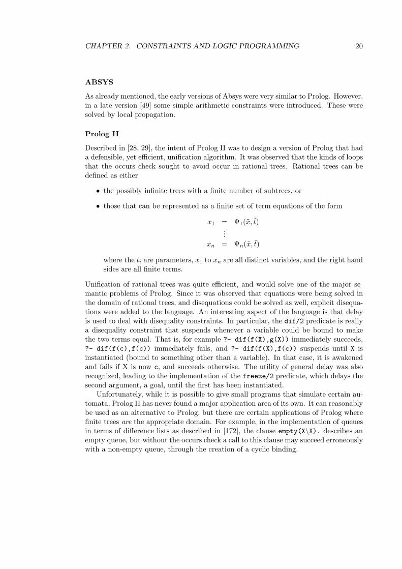
ABSYS
As already mentioned, the early versions of Absys were very similar to Prolog. However,in a late version [49] some simple arithmetic constraints were introduced. These weresolved by local propagation.
Prolog II
Described in [28, 29], the intent of Prolog II was to design a version of Prolog that hada defensible, yet efficient, unification algorithm. It was observed that the kinds of loopsthat the occurs check sought to avoid occur in rational trees. Rational trees can bedefined as either
• the possibly infinite trees with a finite number of subtrees, or
• those that can be represented as a finite set of term equations of the form
x1 = Ψ1(x, t)...
xn = Ψn(x, t)
where the ti are parameters, x1 to xn are all distinct variables, and the right handsides are all finite terms.
Unification of rational trees was quite efficient, and would solve one of the major se-mantic problems of Prolog. Since it was observed that equations were being solved inthe domain of rational trees, and disequations could be solved as well, explicit disequa-tions were added to the language. An interesting aspect of the language is that delayis used to deal with disequality constraints. In particular, the dif/2 predicate is reallya disequality constraint that suspends whenever a variable could be bound to makethe two terms equal. That is, for example ?- dif(f(X),g(X)) immediately succeeds,?- dif(f(c),f(c)) immediately fails, and ?- dif(f(X),f(c)) suspends until X isinstantiated (bound to something other than a variable). In that case, it is awakenedand fails if X is now c, and succeeds otherwise. The utility of general delay was alsorecognized, leading to the implementation of the freeze/2 predicate, which delays thesecond argument, a goal, until the first has been instantiated.
Unfortunately, while it is possible to give small programs that simulate certain au-tomata, Prolog II has never found a major application area of its own. It can reasonablybe used as an alternative to Prolog, but there are certain applications of Prolog wherefinite trees are the appropriate domain. For example, in the implementation of queuesin terms of difference lists as described in [172], the clause empty(X\X). describes anempty queue, but without the occurs check a call to this clause may succeed erroneouslywith a non-empty queue, through the creation of a cyclic binding.
CHAPTER 2. CONSTRAINTS AND LOGIC PROGRAMMING 21
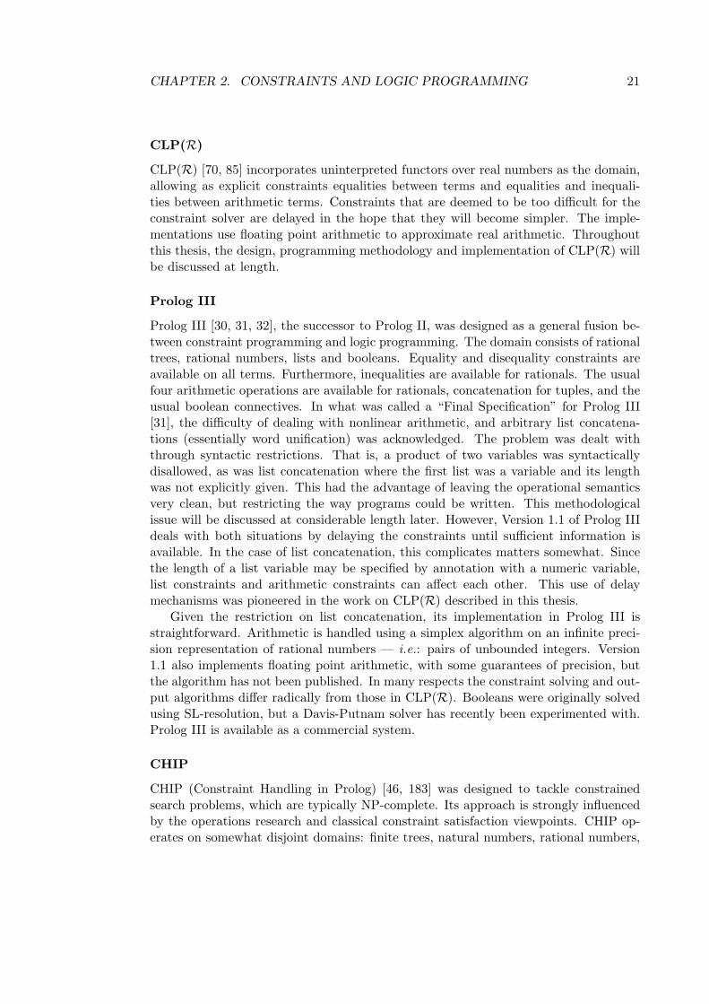
CLP(R)
CLP(R) [70, 85] incorporates uninterpreted functors over real numbers as the domain,allowing as explicit constraints equalities between terms and equalities and inequali-ties between arithmetic terms. Constraints that are deemed to be too difficult for theconstraint solver are delayed in the hope that they will become simpler. The imple-mentations use floating point arithmetic to approximate real arithmetic. Throughoutthis thesis, the design, programming methodology and implementation of CLP(R) willbe discussed at length.
Prolog III
Prolog III [30, 31, 32], the successor to Prolog II, was designed as a general fusion be-tween constraint programming and logic programming. The domain consists of rationaltrees, rational numbers, lists and booleans. Equality and disequality constraints areavailable on all terms. Furthermore, inequalities are available for rationals. The usualfour arithmetic operations are available for rationals, concatenation for tuples, and theusual boolean connectives. In what was called a “Final Specification” for Prolog III[31], the difficulty of dealing with nonlinear arithmetic, and arbitrary list concatena-tions (essentially word unification) was acknowledged. The problem was dealt withthrough syntactic restrictions. That is, a product of two variables was syntacticallydisallowed, as was list concatenation where the first list was a variable and its lengthwas not explicitly given. This had the advantage of leaving the operational semanticsvery clean, but restricting the way programs could be written. This methodologicalissue will be discussed at considerable length later. However, Version 1.1 of Prolog IIIdeals with both situations by delaying the constraints until sufficient information isavailable. In the case of list concatenation, this complicates matters somewhat. Sincethe length of a list variable may be specified by annotation with a numeric variable,list constraints and arithmetic constraints can affect each other. This use of delaymechanisms was pioneered in the work on CLP(R) described in this thesis.
Given the restriction on list concatenation, its implementation in Prolog III isstraightforward. Arithmetic is handled using a simplex algorithm on an infinite preci-sion representation of rational numbers — i.e.: pairs of unbounded integers. Version1.1 also implements floating point arithmetic, with some guarantees of precision, butthe algorithm has not been published. In many respects the constraint solving and out-put algorithms differ radically from those in CLP(R). Booleans were originally solvedusing SL-resolution, but a Davis-Putnam solver has recently been experimented with.Prolog III is available as a commercial system.
CHIP
CHIP (Constraint Handling in Prolog) [46, 183] was designed to tackle constrainedsearch problems, which are typically NP-complete. Its approach is strongly influencedby the operations research and classical constraint satisfaction viewpoints. CHIP op-erates on somewhat disjoint domains: finite trees, natural numbers, rational numbers,

CHAPTER 2. CONSTRAINTS AND LOGIC PROGRAMMING 22
booleans and finite sets of constants or natural numbers.The novel aspect of the language is how it deals with the finite sets. That is, clas-
sical constraint satisfaction problems are encoded as sets of constraints over variableswhose values are known to lie within these finite sets. Rather than using the temporalbacktracking of Prolog, which leads to a generate-and-test search, the forward checking,lookahead and partial lookahead rules of classical CSP are used. These are known asconsistency techniques [112]: a priori pruning, using constraints to reduce the searchspace before discovering a failure.
Variables that take their values from finite sets are known as “domain” variables —not to be confused with the generic use of the term “domain”. Natural number termsconsist of natural numbers, domain variables over natural numbers, and terms builtup from the usual natural number operators. Consistency techniques are used to solveequations, inequalities and disequalities on natural number terms, symbolic constraintson domain variables, and user-defined constraints. The user declares certain predicatesto be suitable as constraints for forward checking purposes if they satisfy a certaincalling pattern. Then these are used in addition to primitive constraints for pruningthe search space.
CHIP has been used for a large number of classical operations research problemswith remarkable success. The implementation of a CHIP compiler was described byAggoun and Beldiceanu in [1], and this provides a useful contrast with the design of theConstraint Logic Arithmetic Machine (CLAM) for CLP(R) compilation as describedin this thesis. In particular, the CHIP compilation model does not allow for many lowlevel optimizations of constraint solving to be expressed.
CAL
CAL [151] is actually a pair of languages using Grobner bases techniques to solve con-straints. Boolean CAL uses a special modification of the Buchberger algorithm forboolean constraints. In real CAL, polynomial equations are solved using the classicalBuchberger algorithm for complex numbers. This is rather problematic, since unsatis-fiability in complex numbers implies unsatisfiability in real numbers, but the conversedoes not hold. It is not satisfactory to simply say that it is a CLP language on complexnumbers, however. In particular, the applications that the authors wish to addressinclude robotics, where the existence of imaginary solutions is far from useful in manycases.
RISC-CLP(R)
Another system dealing with nonlinear arithmetic constraints, based on partial cylin-drical algebraic decomposition and Grobner bases is described by Hong [75]. The aboveconcern about complex numbers is avoided by using the unsatisfiability in the complexdomain only for pruning. This work is only preliminary, and the practicality of theapproach has not yet been established.

CHAPTER 2. CONSTRAINTS AND LOGIC PROGRAMMING 23
BNR Prolog
BNR Prolog [133] was developed by Bell Northern Research, in Canada. It providesarithmetic constraints on closed intervals of the real line. The motivation is to makereal relational arithmetic sound, which it is usually not when floating point arithmeticis used. An unconstrained variable begins as the entire real line (or really boundedby the highest and lowest machine real) and constraints result in this interval beingnarrowed. It is possible that an interval will be narrowed to a point. To maintainsoundness, intervals are always rounded “outwards” when an arithmetic operation isperformed. Iterative solution techniques are used for nonlinear constraints.
Trilogy
Trilogy [103, 185, 186] has an operational model that is substantially divorced fromlogic programming. Prolog-like rules are combined with procedures of conventionalprogramming paradigms. Linear equations and inequalities are solved in the domain ofintegers (Pressburger arithmetic). Mode declarations are used. It is available cheaplyas a commercial product for personal computers.
λProlog and Elf
For our purposes, both λProlog [126] and Elf [139] can be seen as solving equationsbetween terms of the λ-calculus with simple types and dependent types, respectively.The motivation for λProlog was meta-programming for both programming languagesand logics. It is particularly suited to this application as variables in an object languagecan be represented using abstraction in the meta language. Elf does not have predi-cate variables of λProlog, but programs may reason about their partial correctness bymanipulating proofs of sub-goals in a way that is guaranteed to be type correct.
CLP(Σ∗)
The domain of CLP(Σ∗) [187] is regular sets. The language is intended to providea logic-based formalism for incorporating string handling and even file handling intologic programming. The author also points out that problems in computer securitycan be solved by reasoning with regular expressions. The atomic constraints of thelanguage are of the form x in e where x is either a variable or a string, and e is aregular expression possibly containing variables. Where such a constraint can havemultiple solutions, these are dealt with through backtracking. This brings up issuesof scheduling, since constraints may have infinitely many solutions. The schedulingstrategy allows only constraints capable of generating a finite set of solutions to beselected from a conjunction for evaluation. That is, others are essentially delayed. Thisensures termination of unsatisfiable conjunctions.

CHAPTER 2. CONSTRAINTS AND LOGIC PROGRAMMING 24
CIL
CIL (Complex Indeterminate Language) [124, 125] is designed for natural languageprocessing. It is a CLP language over partially tagged trees (PTTs). The terms arecalled Partially Specified Terms (PSTs), which have been described [3] as being exactlythe same as feature matrices used in Unification Grammars [159]. CIL incorporates thefreeze/2 predicate of Prolog II.
LOGIN and LIFE
LIFE [3] is a language consisting of logic programming, functional programming anda facility for structured type inheritance — the ψ-calculus. The logic programmingcomponent together with the ψ-calculus is a CLP language over what are called ψ-terms, and the subtyping and type intersection operations of the ψ-calculus. Thislanguage is called LOGIN [4]. A ψ-term is essentially a data structure built out ofconstructors and access functions, and subject possibly to some equational constraintsthat reflect sharing of structure. In this way the calculus formalizes data structureinheritance.
CLPS
The CLP Shell, described by Lim and Stuckey [109] is an interesting and potentiallyvaluable alternate approach to the systems discussed above. The objective of CLPS is toallow multiple constraint solvers to be incorporated into a CLP system with minimumeffort. However, it remains to be shown that the overhead resulting from this loosecoupling of constraint solvers is not excessive. The promise stems from the fact thatthe system may be useful for prototyping if the overhead is less than say an order ofmagnitude.
Concurrent Constraint Programming, and the Ask/Tell Framework
Concurrent Constraint (CC) programming [152] grew out of the work on committedchoice logic programming languages [156], such as Concurrent Prolog [155]. These lan-guages differ from normal logic programming in that they don’t have the usual “don’tknow” nondeterminism. Instead, they use what is called “don’t care” nondetermin-ism. That is, all clauses for a given predicate are tried concurrently, until one of themreaches a commit operation, at which time the other alternatives are discarded. Com-mitted choice languages originally depended on complicated and cumbersome methodsof synchronization. The idea of concurrent constraint programming was to deal withthis problem by making synchronization dependent on whether some constraint wasentailed by a global constraint store. Such constraints are “Ask” constraints. Thisglobal store is maintained by combining constraints asserted throughout the program– “Tell” constraints. The view of constraints in CC languages is rather different fromthat of this thesis, because entailment rather than (un)satisfiability is used to controlexecution. This view of constraints gives rise to an interesting and challenging set of

CHAPTER 2. CONSTRAINTS AND LOGIC PROGRAMMING 25
design and implementation problems quite different from the ones discussed in thisthesis.
2.3.3 Applications
In recent years, considerable work has been done on applications of various CLP lan-guages. One of the major application areas has been electrical circuit analysis, synthesisand diagnosis [59, 123, 163, 165, 164, 166, 162, 167]. Civil engineering [102] and me-chanical engineering [173] have also attracted some attention. Engineering applicationstend to combine hierarchical composition of complex systems, mathematical or booleanmodels, and — especially in the case of diagnosis and design — deep rule-based rea-soning. Another major area has been that of options trading [74, 78, 79, 104] andfinancial planning [12, 13, 14, 19]. These applications have tended to take the form ofexpert systems involving mathematical models. More traditional operations researchproblems have included cutting stock [44] and scheduling [45].
More exotic applications areas have included restriction site mapping in genetics[192]. Levitt surveyed the use of constraint languages in music [107], and Tobias im-plemented an expert system for tutoring about harmony in CLP(R) [182]. CLP(R)was also used for generating test data for communications protocols [57]. Prolog wasdeveloped by the Marseille group for natural language processing, so it should come asno surprise that this is turning out to be significant application area for LIFE [3], CIL[125], Prolog III [31] and λProlog [120, 34]. Both λProlog [62] and Elf [117] have beenused for implementing natural semantics of programming languages. λProlog has alsobeen used for implementing natural deduction-style theorem provers [52]. Applicationsof CLP(R), λProlog and Elf will be discussed in more detail in Part II.

Part II
Languages and Programming
26

Chapter 3
Language Design
To design a CLP language, it is necessary to choose a domain of computation. Recallthat choosing a domain involves choosing the underlying set of values with which weare computing, the expressions (operations) allowed on that set, and the constraintsallowed on variables ranging over the set. As we shall see, the major theme of CLPlanguage design is introducing suitable compromises, based on complications result-ing from implementation issues. Furthermore, it is necessary for compromises to beintroduced to the operational model as well.
It is also important to consider what minimum domain is necessary to provideenough utility to solve the required class of problems. In particular, most CLP lan-guages should probably include uninterpreted functors, thus at least nominally makingProlog a subset. This makes a language more amenable to “general purpose” pro-gramming, providing at least basic data structuring mechanisms. As a medium termconsideration, in order for CLP to be adopted into the applications community, itwill be necessary to promote the languages as extensions of Prolog, which run Prologprograms essentially without modification, and with more or less the usual efficiency.
For the purposes of the following discussion, we define a CLP program as being afinite set of rules of the form
A :– γ1, · · · , γn, n ≥ 0
where A is an atom and each γi is either a constraint or an atom. An atom consists of apredicate symbol with the appropriate number of terms as arguments, and a constraintis a constraint symbol with the appropriate number of terms as arguments. A term isbuilt up from variables and constants and function symbols from the domain.
3.1 CLP Operational Model
We begin by formally defining a CLP operational model, with enough generality toaccount for compromises motivated by implementation concerns. Inherent in the oper-ational model of CLP is a subgoal selection strategy, which selects a delayed constraintor an atom from a given goal. Now let P denote a CLP program. Let G denote a
27

CHAPTER 3. LANGUAGE DESIGN 28
goal consisting of a sequence γ1, · · · , γl and a function partitioning this sequence intomultisets Λ of atoms, Σ of solved constraints and ∆ of delayed constraints. In an initialgoal, all the constraints are delayed (in ∆). We say that there is a derivation step fromG to another goal G2 if the subgoal selection strategy selects some γi for 1 ≤ i ≤ l andone of the following holds:
• γi ∈ ∆ and Σ ∪ γi is satisfiable.Then G2 is the sequence G with partition Λ2 = Λ, ∆2 = ∆ \ γi and Σ2 =Σ ∪ γi.
• γi ∈ Λ and the program P contains a rule R that can be renamed so that itcontains only new variables and takes the form: the head atom is H, the body isthe sequence denoted by B1, B2, . . . , Bs, s ≥ 0, partitioned similarly into multisetsΛ1 and ∆1.Then G2 is the sequence γ1, . . . , γi−1, γi = H1, B1, . . . , Bs, γi+1 . . . , γn, with thepartition Σ2 = Σ, ∆2 = ∆ ∪∆1 ∪ γi = H and Λ2 = (Λ \ γi) ∪ Λ1.
We say that γi in G above is the selected subgoal. Equivalently, γi is the subgoal of Gchosen to be reduced.
A derivation sequence (or simply sequence) is a possibly infinite sequence of goals,starting with an initial goal, wherein there is a derivation step to each goal from thepreceding goal. A sequence is successful if it is finite and its last goal contains onlysolved constraints. A sequence is conditionally successful if it is finite and its lastgoal contains only solved and delayed constraints. Finally, a finitely failed sequenceis finite, neither successful nor conditionally successful, and such that no derivationstep is possible from its last goal2. The constraints in the last goal of successful andconditionally successful sequences are called answer constraints, and they constitutethe output of CLP programs.
Thus a program and goal are executed by a process of continuously reducingany remaining atoms or solving delayed constraints in the goal. There are two non-deterministic aspects in obtaining a derivation sequence from a given initial goal as wehave defined above. One pertains to the subgoal selection strategy, The other pertainsto the search strategy, which determines which rule is used next in the reduction of aselected atom in a subgoal.
As an example, consider the following program solving real arithmetic constraints.
ohm(V, I, R) :- V = I * R.
The following, in which we indicate solved constraints by underlining them, illustratesa successful derivation sequence:
1This abbreviates the collection of equations between corresponding arguments in γi and H.2If the subgoal selection strategy is fair in the sense that every delayed constraint and atom in an
infinite sequence is eventually selected, then one has the usual soundness and completeness results withrespect to successful and finitely failed sequences [82].
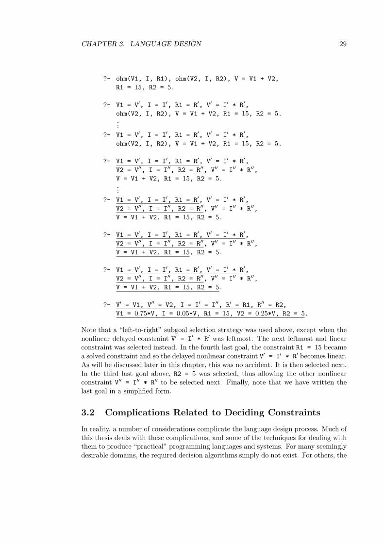
CHAPTER 3. LANGUAGE DESIGN 29
?- ohm(V1, I, R1), ohm(V2, I, R2), V = V1 + V2,R1 = 15, R2 = 5.
?- V1 = V′, I = I′, R1 = R′, V′ = I′ * R′,ohm(V2, I, R2), V = V1 + V2, R1 = 15, R2 = 5....
?- V1 = V′, I = I′, R1 = R′, V′ = I′ * R′,ohm(V2, I, R2), V = V1 + V2, R1 = 15, R2 = 5.
?- V1 = V′, I = I′, R1 = R′, V′ = I′ * R′,V2 = V′′, I = I′′, R2 = R′′, V′′ = I′′ * R′′,V = V1 + V2, R1 = 15, R2 = 5....
?- V1 = V′, I = I′, R1 = R′, V′ = I′ * R′,V2 = V′′, I = I′′, R2 = R′′, V′′ = I′′ * R′′,V = V1 + V2, R1 = 15, R2 = 5.
?- V1 = V′, I = I′, R1 = R′, V′ = I′ * R′,V2 = V′′, I = I′′, R2 = R′′, V′′ = I′′ * R′′,V = V1 + V2, R1 = 15, R2 = 5.
?- V1 = V′, I = I′, R1 = R′, V′ = I′ * R′,V2 = V′′, I = I′′, R2 = R′′, V′′ = I′′ * R′′,V = V1 + V2, R1 = 15, R2 = 5.
?- V′ = V1, V′′ = V2, I = I′ = I′′, R′ = R1, R′′ = R2,V1 = 0.75*V, I = 0.05*V, R1 = 15, V2 = 0.25*V, R2 = 5.
Note that a “left-to-right” subgoal selection strategy was used above, except when thenonlinear delayed constraint V′ = I′ * R′ was leftmost. The next leftmost and linearconstraint was selected instead. In the fourth last goal, the constraint R1 = 15 becamea solved constraint and so the delayed nonlinear constraint V′ = I′ * R′ becomes linear.As will be discussed later in this chapter, this was no accident. It is then selected next.In the third last goal above, R2 = 5 was selected, thus allowing the other nonlinearconstraint V′′ = I′′ * R′′ to be selected next. Finally, note that we have written thelast goal in a simplified form.
3.2 Complications Related to Deciding Constraints
In reality, a number of considerations complicate the language design process. Much ofthis thesis deals with these complications, and some of the techniques for dealing withthem to produce “practical” programming languages and systems. For many seeminglydesirable domains, the required decision algorithms simply do not exist. For others, the

CHAPTER 3. LANGUAGE DESIGN 30
decision problem may be open. It is then necessary to decide whether undecidabilityis expected to be a problem in practice. For many more domains, either the decisionproblem is known to be intractable, or the best known algorithms are impractical. Evenwhen a reasonably (or very) efficient decision procedure exists, it may be incompatiblewith the CLP operational model. In particular, a CLP implementation requires incre-mental satisfiability testing to be efficient. That is, it must be possible to determineefficiently whether a satisfiable set of constraints, augmented with a new constraint,is still satisfiable. Efficiency here loosely means that the time should be proportionalmore to the size of the added constraint than that of the previous, satisfiable, set. Fur-thermore, because of backtracking, it must be possible to undo such augmentations ofthe constraint set efficiently.To make the above more concrete, let us consider a number of examples.
• Natural numbers and integers are useful domains for many applications of anoperations research flavor. Nonlinear polynomial equations over integers, knownmore commonly as diophantine equations, are undecidable. Linear equations andinequalities are decidable but expensive to decide.
• Equations between simply-typed λ-expressions are undecidable.
• Real polynomial equations and inequalities are decidable, but all known algo-rithms are extremely inefficient. Real linear equations and inequalities are effi-ciently decidable: polynomial algorithms are known, and some are even knownto be efficient in practice.
• A linear algorithm for unification of finite trees is available: one was described byPaterson and Wegman in [136] However, no linear unification algorithm is knownto perform well in practice. It is instructive to notice that the usual (Robinson)algorithm for unification of finite trees, as implemented in most Prolog systems,is quite incremental in practice. The cost of backtracking is linear in the numberof variables instantiated since the last choicepoint, and unification cost is onlysomewhat dependent on the number of prior constraints (as instantiated variablesare more costly to unify than free ones, since they have to be traversed). TheRobinson algorithm is, depending on how terms and unifiers are represented,either exponential or polynomial in the worst case.
3.3 Effect on Language Design
Issues of incremental satisfiability are discussed further in Chapter 9. Where an efficientincremental solver is not readily available, the problems discussed above can often bedealt with by appropriate restriction and organization of constraint solvers. To applythese techniques, the design of a CLP language must begin with an intended applicationarea (or areas) and programming style. If constraint solving is to be restricted, certainkinds of constraints must be identified as being too difficult to solve in the general case.In this thesis they will be called the hard constraints. We now consider various ways

CHAPTER 3. LANGUAGE DESIGN 31
to deal with hard constraints, given that the domain of computation is general enoughthat such constraints can be expressed in the language.
3.3.1 Syntactic Restrictions
One approach is to syntactically restrict the kinds of constraints on the given domainthat can be expressed. Note that the domain itself specifies the operations and relationson the underlying set that are allowed. The syntactic restrictions here determine whatexpressions can be built up using the operators, and what expressions the variousrelation symbols can be applied to. Let us consider some examples.
• Arithmetic expressions can be restricted to being linear, by requiring that multi-plication only occur between two constants or between a constant and a variable,but not between two variables.
• Simply-typed λ-expressions can be restricted essentially such that, for example,one existentially quantified variable cannot be applied to another. The detaileddefinition of the restricted language, and the significance of the restriction, willbe discussed in Chapter 5.
• Word equations can be restricted to avoid the case where the length of an initialvariable is unknown.
• Consider linear equations and inequalities on reals or rationals. Shostak [161]gave a decision algorithm based on computing loop residues that is particularlyefficient when there are no more than two variables per constraint (note that threevariables per constraint are sufficient to express any set of constraints).
The syntactic restrictions should be such that they still enable the programmer toexpress what is needed. As a result, not all problems of undecidability or inefficiencycan be handled in this way. One reasonable alternative is to insist that the expressibleconstraints should at least be decidable. However, even this restriction is sometimesexcessive, as is the case with λProlog and Elf, which will be discussed in Chapters 5and 11. At the very least, the language should be restricted sufficiently as to make thedynamic restriction techniques discussed below applicable and useful. It turns out thatsyntactic restriction is usually an excessively brutal way to obtain an efficiently imple-mentable programming language. This is because constraints that appear syntacticallycomplex can often be simplified considerably by the time they are selected at runtime.These observations will be discussed in more detail in the next two chapters.
3.3.2 Dynamic Restrictions
In the philosophy of constraint programming it is important that the programmershould not have to be concerned with when information becomes available but justneeds to provide enough constraints for it eventually to become available. A moreeffective way to cut the constraints down to size, then, is to restrict them dynamically.

CHAPTER 3. LANGUAGE DESIGN 32
That is, impose conditions on the form of a constraint when it is selected, rather thanwhen it is parsed. By the time a constraint is selected, some of its variables may havebeen involved in a number of other constraints. Thus enough may be known aboutthem that deciding the constraint has become much simpler than might be expectedby examining it syntactically, in isolation. For example, a nonlinear arithmetic equationmight be made linear by the grounding of one or more variables. Or an equation betweentwo simply-typed λ expressions might similarly become deterministic. Of course, weshould note that this discussion hinges on the language designer having a clear ideaabout the programming methodology that the language is intended to support. Thisissue will be discussed in some detail in the next two chapters.
There are two possible ways to deal with the situation where a constraint is selectedand does not meet the appropriate syntactic requirements.
• Runtime errorHalt execution of the program, and print an error message, hopefully giving in-formation on how the restriction was not satisfied.
• DelayAssume, for the time being, that the constraint is consistent with the collectedconstraints, but do not solve it – just store it. Then if it later does satisfy therestriction, add it, and backtrack if it is inconsistent.
The first approach is the usual way to deal with system predicates in Prolog. Forexample, in most Prolog systems,
?- X = 1, Y = 3, Z is X + Y.
binds Z to 4, while
?- X = 1, Z is X + Y, Y = 3.
will cause a runtime error when Z is X + Y is selected, as Y is still free. This is certainlyan improvement on static restrictions. For example, in a CLP language dealing withreals, consider the following constraints with a left-right atom selection rule.
?- I1 + I2 = 10, I1 - I2 = 0, V = I2 * R + 2 * I2 * R.
By the time the third constraint is selected, I1 and I2 have values, so the equationis linear. However, such a restriction still places on the programmer the burden ofworrying about when information becomes available, rather than just that of givingenough information.
Delay mechanisms have quite a long history in logic programming: a systematicstudy by Naish can be found in [128]. They have most commonly been used to delaythe calling of certain subgoals, either by annotating the subgoal with a delay condition,or by annotating the rules defining a given predicate with the condition. Prolog II’sfreeze/2 predicate is an example of the former, and the wait declarations of MU-Prolog and when declarations of Nu-Prolog are examples of the latter. MU-Prolog and

CHAPTER 3. LANGUAGE DESIGN 33
Nu-Prolog also use delay on certain system predicates, such as a special predicate formultiplication by local propagation. Carlsson [22] described how such general delaymechanisms could be implemented efficiently. To see the advantages of delay mecha-nisms for constraints, consider a permuted version of the example above, and assumethat nonlinear equations and inequalities are delayed until they become linear.
?- V = I2 * R + 2 * I2 * R, I1 + I2 = 10, I1 - I2 = 0.
Here the first equation can simply be delayed when selected, and when the values of I1and I2 are obtained from the subsequent constraints, it can be “awakened”. Deeperexamples of this phenomenon in real programs will be discussed in Chapter 4. As anexample in a different domain, let us consider word equations. The goal
?- X.Y = abcde, Y = c.Z .
has the unique answer
X = ab, Y = cde, Z = de
But if constraints are delayed until the variable on the left of a concatenation is ofknown length, the constraints will not produce an answer. However, the goal
?- X.Y = abcde, Y = c.Z, |Z| = 2.
can obtain the answer using delay as follows.
• After the first constraint is delayed, additional constraints are established:
|X| + |Y| = 5, |X| <= 5, |X| >= 0
• After the second constraint is encountered, the first cannot yet be awakened butadditional (arithmetic) constraints are established:
|X| + |Z| = 4, |X| <= 4, X.c.Z = abcde
• Finally, the addition of the third constraint makes it possible to infer the con-straint
|X| = 2
so the first constraint can be awakened, binding X to ab and Y to cde.
The interested reader can find similar examples for CLP(Σ∗) in [187].Delay gives the programmer considerable flexibility, but also additional responsibil-
ity. For a start it is now possible to obtain deadlock — a situation where only delayedconstraints remain, but none meets the selection criteria. This might be considered anerror condition, or the notion of termination might be extended to include the possibil-ity of a deadlocked computation, where the answer to the query is maybe. The answer

CHAPTER 3. LANGUAGE DESIGN 34
constraint could then be printed, with its correctness being contingent on the (undeter-mined) satisfiability of the delayed constraints. Additional problems of programmingmethodology arise when this approach is chosen. In particular, the programmer isnot really freed from the burden of understanding when information becomes available.Where constraint (un)satisfiability is used to control search, an inconsistency that isdetected too late can lead to an infinite loop, both in cases when the query should havesucceeded, and in cases where it should have failed finitely. Such a delay mechanismcan thus lead to rather insidious bugs in a program. These problems are partially illus-trated by the following definitions of the predicates silly and dangerous. We againassume that nonlinear equations and inequalities are delayed until enough informationis available to make them linear.
silly(X) :- X*X < 10, X > 4, loopalways(X).
dangerous(X) :- X*X < -5, loopalways(X).dangerous(3).
Any call to silly should simply fail, since the two constraints are inconsistent. How-ever, if X is free in the call, the first constraint will be delayed, and the second does notproduce enough information to awaken it. Hence the call to loopalways will happen,producing an infinite loop. A call to dangerous with a free value of X should succeed,binding X to 3, as the constraint is unsatisfiable. However, such a call will result in theconstraint being delayed, thus ending up in an infinite loop. Of course, it should bepointed out that the problem we are describing is not new: the operational model ofProlog itself introduces very similar problems.
The issue of how to restrict a CLP language appropriately has often come up andbeen addressed in different ways in real systems. As will be discussed in some detail inChapter 4, in CLP(R) the selection rule is modified to delay nonlinear constraints untilthey become linear. In the early documents on Prolog III on the other hand, includingthe so-called “Final Specification” [31], the syntactic approach to this same problemwas strongly advocated, although the claims of this thesis about the methodologicaladvantages of delay, had already been made. However, recent commercial versions ofProlog III employ delay for nonlinears also. Furthermore, the same approach is nowused in Prolog III to deal with the intractability of word unification. A word equation isdelayed until the length of any initial variables is known. (In fact, at the implementationlevel, it delays them until it is known whether the length of the leading variable is zeroor non-zero [33]. As will be discussed in subsequent chapters, a similar argument hasoccurred over how the non-determinism of higher-order unification should be handled.Likewise, a delay approach could be applied to constraints on data aggregates, such asarrays. These examples will be discussed in more detail in Chapter 7.
It should be noted that even for applications that can run correctly with certaindynamic restrictions, these might have an adverse effect. For example, in Chapter 4a crypto-arithmetic program is discussed that uses linear inequalities heavily. If onlyequations were decided, and inequalities were delayed until ground, this program wouldstill run correctly. However, an important trade off exists in terms of efficiency: deciding

CHAPTER 3. LANGUAGE DESIGN 35
linear inequalities causes earlier pruning of the search space, but is considerably morecostly per constraint. Thus which approach is faster actually depends on the numberof constraints pruned versus the cost of solving an inequality.
Delay mechanisms, of course, bring their own implementation difficulties, althoughdelaying constraints is not as problematic as delaying general calls, as described in [22].For the operational model to be reasonably intuitive for the programmer, it is necessaryto awaken delayed constraints as soon as possible after they become sufficiently simple.However, on backtracking, an awakened constraint must be resuspended. Naturally,backtracking complicates any indexing structures that are used for timely awakening.Of course there is an overhead associated with checking for awakened constraints when-ever the constraint store is augmented, but this can usually be kept low. These issuesare discussed in detail in Chapter 7.
3.4 Looking Ahead
The role of the next two chapters, about language design and programming method-ology aspects of CLP(R), λProlog and Elf, make the assertions of this chapter at amore concrete level. All three languages are now well-enough understood and are usedwidely enough that some quite specific comments can be made about the interactionbetween language design and programming methodology. One of the claims of thisthesis is that the pragmatic approach to designing CLP languages through restrictingconstraint solving by delay provides the right compromise between expressive powerand efficiency.

Chapter 4
CLP(R)
The design and implementation of a CLP language for real arithmetic was essentiallymotivated by two observations:
• Real arithmetic is of fundamental importance in computer science, simply becauseof the demands of applications.
• Historically, many declarative programming languages have not dealt well witharithmetic.
In particular, real arithmetic was grafted onto most Prolog systems at an early stage,but in a form that ran counter to the philosophy of logic programming. This wasusually in the form of the two-argument is predicate, which evaluated the arithmeticexpression in its second argument, expecting all the variables in the expression to havealready been bound to numbers, and assigning the resulting value to the free variablein the first argument. That is, arithmetic was essentially handled in the same way asin imperative languages. The following discussion introduces CLP(R), a systematicattempt to use the CLP framework to produce a language with real arithmetic thatmaintains the advantages of the logic programming framework. This is followed by anextensive discussion of programming methodology, together with empirical observationsabout the kinds of constraint solving that are required in typical programs. A discussionof some relatively large scale applications is included.
4.1 The Language and Operational Model
We now describe the syntax of CLP(R) programs and their intuitive semantics. Thenwe describe the operational model of the CLP(R) system, an approximation to themodel prescribed by the CLP scheme as described in Chapter 3.
4.1.1 The Structure REssentially,R is a two-sorted structure where one sort is the real numbers, and the othersort is the set of trees over uninterpreted functors and real numbers. The construction
36

CHAPTER 4. CLP(R) 37
of trees using uninterpreted functors is the only tree operation. The only real numberoperations are addition and multiplication. While equality is the only relation betweentrees, both equality and inequality are defined on numbers. The truth of these relationsis defined in the obvious way: two trees are equal iff their root functors are the sameand their corresponding subtrees, if any, are equal. The truth of real number relationsis defined in the standard way.
We now proceed with the syntactic formulation of R. In what follows, we shallassume tacitly, to avoid further formality, that the language CLP(R) is (statically)typed in the sense that the type (real number or functor) of each argument of eachpredicate symbol and functor, as well as the type of each variable, is pre-determined.In CLP(R) programs, therefore, each predicate symbol, functor and variable is used ina consistent way with respect to its type.
4.1.2 CLP(R) Constraints
Real constants and real variables are both arithmetic terms. If t1, t2 are arithmeticterms, then so are (t1 + t2), (t1− t2) and (t1 ∗ t2). Uninterpreted constants and functorsare like those in Prolog. Uninterpreted constants and arithmetic terms are terms, andso is any variable. The rest of the terms are defined inductively as follows: if f is ann-ary uninterpreted functor and t1, ..., tn are terms, then f(t1, ..., tn) is a term.
If t1 and t2 are arithmetic terms, then t1 = t2, t1 < t2 and t1 ≤ t2 are all arithmeticconstraints. If, however, not both the terms t1 and t2 are arithmetic terms, then onlythe expression t1 = t2 is a constraint. Both these kinds of constraints will be used inprograms, and they form a subset of all the predicates that may appear in a program.Because these constraints have pre-defined meanings, we shall sometimes emphasize thisby calling them primitive constraints (or simply constraints when confusion is unlikely).A primitive constraint is solvable iff there is an appropriate assignment of real numbersand ground terms to the variables therein such that the constraint evaluates to true.
In what follows, we adopt the (Prolog) convention of using strings beginning withcapital letters to denote variables.
4.1.3 CLP(R) Programs
An atom is of the form p(t1, t2, . . . , tn) where p is a predicate symbol distinct from =,<, and ≤, and t1, ..., tn are terms. A rule is of the form
A0 :– α1, α2, . . . , αk.
where each αi, 1 ≤ i ≤ k, is either a primitive constraint or an atom. The atom A0
is called the head of the rule while the remaining atoms and primitive constraints areknown collectively as the body of the rule. In case there are no atoms in the body, wemay call the rule a fact or a unit rule. In case there are no atoms and constraints inthe body, we may abbreviate the rule to be simply of the form
A0.

CHAPTER 4. CLP(R) 38
Finally, a CLP(R) program is defined to be a finite collection of rules.Thus rules in CLP(R) have much the same format as those in Prolog except that
primitive constraints may appear together with atoms in the body. The same appliesto a CLP(R) goal; this is of the form
?– α1, α2, . . . , αk.
where each αi, 1 ≤ i ≤ k, is either a primitive constraint or an atom. A sub-collectionof the atoms and constraints in a goal is sometimes called a subgoal of the goal.
The following is a CLP(R) program for computing Fibonacci numbers:
fib(0, 1).fib(1, 1).fib(N, X1 + X2) :-
N > 1,fib(N - 1, X1),fib(N - 2, X2).
Its declarative semantics is clear. A goal that asks for a number A such that fib(A)lies in between 80 and 90 is
?- 80 <= B, B <= 90, fib(A, B).
and, as will be shown next, the answer obtained when the program and goal are executedis A = 10, B = 89.
We conclude this subsection with another example program:
available res(10).available res(14).available res(27).available res(60).available res(100).
available cell(10).available cell(20).
ohm(V, I, R) :- V = I * R.
sum([], 0).sum([H | T], N) :- N = H + M, sum(T, M).
kirchoff(L) :- sum(L, 0).
The program, together with the goal below, represents a simple preferred value problemin which we have an electrical circuit template and can choose from a finite set of

CHAPTER 4. CLP(R) 39
components to select those that make the circuit satisfy a certain property. In thisexample, the simple circuit has two resistors connected in series:
?- 14.5 < V2, V2 < 16.25,available res(R1), available res(R2),available cell(V),ohm(V1, I1, R1), ohm(V2, I2, R2),kirchoff([I1, -I2]), kirchoff([-V, V1, V2]).
The three answer constraints for the program and goal are as follows.
14.5 < V2, V2 < 16.25,V1 / 10 - V2 / 27 = 0,V1 + V2 = 20
14.5 < V2, V2 < 16.25,V1 / 14 - V2 / 60 = 0,V1 + V2 = 20
14.5 < V2, V2 < 16.25,V1 / 27 - V2 / 100 = 0,V1 + V2 = 20
4.1.4 The Operational Model
The operational model presented in Chapter 3 is rather general: unnecessarily so forthis discussion. In discussing CLP(R), we specialize the operational model by specify-ing a left-right subgoal selection strategy for atoms and delayed constraints. That is,considering atoms and delayed constraints as one sequence, these are solved one by onefrom left to right. Recall that in the general CLP operational model, all constraints areinitially considered delayed. Selected constraints that are considered hard (in CLP(R),the nonlinear arithmetic constraints) remain delayed after selection, but are re-selectedas soon as they cease to be hard, in preference to other delayed constraints. Thisspecialized operational model suggests a rather different presentation, as given here.This presentation corresponds more readily to the programmer’s mental view of theexecution of programs.
Now let P denote a CLP(R) program. Let G denote a goal
Σ,∆ ?- A1, A2, . . . , An, n ≥ 0.
where Σ is a set of solved constraints, ∆ is a set of delayed constraints, the Ai areeither atoms or constraints. We say that there is a derivation step from G to anothergoal G2 if one of the following holds:
• Some δ ∈ ∆ is not hard with respect to Σ, and Σ∪δ is solvable. Then G2 is ofthe form
Σ ∪ δ,∆ \ δ ?- A1, A2, . . . , An.

CHAPTER 4. CLP(R) 40
• The first condition does not hold, A1 is a constraint, and is hard with respect toΣ. Then G2 is
Σ,∆ ∪ A1 ?- A2, . . . , An.
Of course, Σ remains solvable.
• The first condition does not hold, A1 is a constraint, is not hard with respect toΣ, and Σ ∪ A1 is solvable. Then G2 is
Σ ∪ A1,∆ ?- A2, . . . , An.
• The first condition does not hold, and A1 is an atom. The program P contains arule R that can be renamed so that it contains only new variables and takes theform
B :- B1, B2, . . . , Bs, s ≥ 0.
Then G2 isΣ,∆ ?- A = B,B1, . . . , Bs, A2, . . . , An
where A = B abbreviates the collection of equations between corresponding ar-guments in A and B. Of course, Σ remains solvable.
In the initial goal, Σ = ∆ = .A derivation sequence (or simply sequence) is a possibly infinite sequence of goals,
starting with an initial goal, wherein there is a derivation step to each goal from thepreceding goal. A sequence is successful if it is finite and its last goal is Σ, ?- . Asequence is conditionally successful if it is finite and its last goal is Σ,∆ ?- where∆ is nonempty. Finally, a finitely failed sequence is finite, neither successful nor condi-tionally successful, and such that no derivation step is possible from its last goal.
As an illustration, we return to the program and query used in Chapter 3, whichhappened to be in CLP(R).
ohm(V, I, R) :- V = I * R.
The successful derivation sequence is shown in Figure 4.1.CLP(R) is an approximation to the operational model of the CLP scheme for four
main reasons:
• To solve equations between non-arithmetic terms, an algorithm similar to a con-ventional unification algorithm is used. No “occurs check” is done, as this issueis largely orthogonal to those of interest.
• As has already been mentioned, a left-right subgoal selection strategy is used, andnonlinear arithmetic constraints are delayed until they become linear. CLP(R)employs a “top-to-bottom” depth-first search strategy in the generation of deriva-tion sequences.

CHAPTER 4. CLP(R) 41
, ?- ohm(V1, I, R1), ohm(V2, I, R2), V = V1 + V2, R1 = 15, R2 = 5., ?- V1 = V′, I = I′, R1 = R′, V′ = I′ * R′,ohm(V2, I, R2), V = V1 + V2, R1 = 15, R2 = 5.
... V1 = V′, I = I′, R1 = R′ , V′ = I′ * R′ ?- ohm(V2, I, R2), V = V1 + V2, R1 = 15, R2 = 5. V1 = V′, I = I′, R1 = R′ , V′ = I′ * R′ ?- V2 = V′′, I = I′′, R2 = R′′, V′′ = I′′ * R′′,V = V1 + V2, R1 = 15, R2 = 5.
... V1 = V′, I = I′, R1 = R′, V2 = V′′, I = I′′, R2 = R′′ , V′ = I′ * R′, V′′ = I′′ * R′′ ?- V = V1 + V2, R1 = 15, R2 = 5. V1 = V′, I = I′, R1 = R′, V2 = V′′, I = I′′, R2 = R′′, V = V1 + V2 , V′ = I′ * R′, V′′ = I′′ * R′′ ?- R1 = 15, R2 = 5. V1 = V′, I = I′, R1 = R′, V2 = V′′, I = I′′, R2 = R′′,V = V1 + V2, R1 = 15 , V′ = I′ * R′, V′′ = I′′ * R′′ ?- R2 = 5. V1 = V′, I = I′, R1 = R′, V2 = V′′, I = I′′, R2 = R′′,V = V1 + V2, R1 = 15 V′ = I′ * R′ , V′′ = I′′ * R′′ ?- R2 = 5. V1 = V′, I = I′, R1 = R′, V2 = V′′, I = I′′, R2 = R′′,V = V1 + V2, R1 = 15 V′ = I′ * R′, R2 = 5 , V′′ = I′′ * R′′ ?- V1 = V′, I = I′, R1 = R′, V2 = V′′, I = I′′, R2 = R′′,V = V1 + V2, R1 = 15 V′ = I′ * R′, R2 = 5, V′′ = I′′ * R′′ ?- V′ = V1, V′′ = V2, I = I′ = I′′, R′ = R1, R′′ = R2,V1 = 0.75*V, I = 0.05*V, R1 = 15, V2 = 0.25*V, R2 = 5 ,?-
Figure 4.1: Successful derivation sequence for ohm query

CHAPTER 4. CLP(R) 42
• A floating-point representation of real numbers is employed. A small and speci-fiable fixed tolerance is used in the comparisons of numbers.
• The constraint solver does not determine the solvability of all nonlinear con-straints.
The first two points pertain to Prolog implementations as much as to CLP(R). The se-lection and search strategies are chosen simply for pragmatic reasons. In short, CLP(R)inherits the approaches to these two issues, as well as the occurs check, from usual Pro-log implementation strategies. The third point, using floating-point numbers, clearlycan give rise to unsoundness. However, our estimation is that alternative implemen-tations (e.g. rational number or interval based methods) are unacceptably costly in ageneral-purpose system. Our experience over many application programs shows thatthe use of floating-point numbers has rarely been problematic, but there is certainlyscope for a CLP system to be developed around some sound form of real arithmetic.
We now discuss the last point in the remainder of this section. As an example ofdelay in CLP(R), the following rule can be used for multiplying or dividing complexnumbers:
c mult(c(R1, I1), c(R2, I2), c(R3, I3)) :-R3 = R1 * R2 - I1 * I2,I3 = R1 * I2 + R2 * I1.
Any of the following goals will return a unique answer:
?- c mult(c(1, 1), c(2, 2), Z).?- c mult(c(1, 1), Y, c(0, 4)).?- c mult(X, c(2, 2), c(0, 4)).
Execution of the first goal is performed by evaluation and assignment in the traditionalway. The other two goals require the division of complex numbers, and the uniqueanswers, one for each of the two cases, can only be obtained by the solution of (two)simultaneous linear equations. Thus none of the three goals above gives rise to anydelayed constraints. The following goal, however, does:
?- c mult(c(X, Y), c(X, Y), c(-3, 4)).
This is because the constraints obtained from expanding this goal are
X*X - Y*Y = -3,2*X*Y = 4.
If, however, this goal also contained an atom or constraint whose expansion or solutiongrounds either X or Y , then a unique answer can be obtained. For example, with therule

CHAPTER 4. CLP(R) 43
p(Y, Z) :- Y = 2*Z, Z = Y-1.
and goal
?- c_mult(c(X, Y), c(X, Y), c(-3, 4)), p(Y, Z).
the call to p gives a value to Y (grounds Y to 2), and so the goal can be executed bythe CLP(R) system to return X = 1, Y = 2, Z = 1.
Clearly the delay/wakeup technique allows the easy introduction of many other(nonlinear) arithmetic functions. For example, it is a trivial matter to augment theCLP(R) system to include the functions sin, cos, abs and pow. We can define that theabs function is delayed until either the input can be evaluated as a ground value, orthe vartiable equated to the output is ground and not positive. Similarly, the equationX = pow(Y, Z), representing X = Y Z , can be defined to awake upon the grounding oftwo of three variables X,Y, Z, or the grounding of Y to 0 or 1, or the grounding of Zto 0 or 1, etc.
4.2 Basic Programming Techniques
We begin this discussion with a number of quite simple programming examples. Thesewill also serve to illustrate a range of CLP(R) programming techniques, and hence laythe foundations for a discussion of programming methodology and later implementa-tion, as well as supporting earlier assertions about language design.
A primitive constraint in a rule typically represents a local property of the sub-problem at hand. While these constraints represent the relationship between variousparameters in a particular part of a problem, (for example, Ohm’s law for a resistorin a circuit), we require global constraints to describe the way these parts interact(for example, the use of Kirchoff’s current law in node analysis). In CLP(R), globalproperties of a problem are represented by means of rules, and the corresponding globalconstraints are those associated with the answer constraints of the program.
The most straightforward way to represent global properties in a program is byhierarchical composition. For example, a rule of the form
p(. . .)← constraints , p1(. . .), . . . , pn(. . .).
can be used where p1, . . . , pn are definitions of largely independent parts of some system,and this rule combines these into a whole by sharing variables in the arguments andvia the list of constraints. As a concrete example, consider the rule
resistor(V, I, R) :- V = I * R.
which describes the local property of a resistor’s voltage/current relationship. Thenthe rules

CHAPTER 4. CLP(R) 44
parallel circuit(V, I, R1, R2) :-I1 + I2 = I,resistor(V, I1, R1),resistor(V, I2, R2).
series circuit(V, I, R1, R2) :-V1 + V2 = V,resistor(V1, I, R1),resistor(V2, I, R2).
combine two resistors to model their behavior in parallel and in series respectively. Thisis achieved in the first case by summing their currents and then using the commonvariable V to constrain the voltage drops across them to be equal. In the second rule,we have the dual situation — a shared variable for current and a constraint for voltage.One can build up more complicated systems by building a multi-level hierarchy ofcomponents. For example, to describe two parallel pairs of resistors in series we maywrite
parallel series(V, I, R1, R2, R3, R4) :-V1 + V2 = V,parallel circuit(V1, I, R1, R2),parallel circuit(V2, I, R3, R4).
While the output of answer constraints is beyond the scope of this thesis, a lotof CLP(R) programming1 is centered around producing such answers. Consider, forexample, the following program, which relates the key parameters in a mortgage:
mortgage(P, Time, I, MP, B):-Time > 0,Time <= 1,Interest = Time * (P * I/1200),B = P + Interest - (Time * MP).
mortgage(P, Time, I, MP, B):-Time > 1,Interest = P * I/1200,mortgage(P + Interest - MP, Time - 1, I, MP, B).
The parameters above are principal (P), life of the mortgage in months (Time), annualinterest rate (%) compounded monthly (I), the monthly payment (MP), and finally, theoutstanding balance (B). The goal
?- mortgage(100000, 360, 12, MP, 0).
asks the straightforward query as to how much it would cost to finance a $100,000mortgage at 12 percent for 30 years, and the answer obtained is MP = 1028.61. The
1See Section 4.4 for a discussion of experience with large amounts of CLP(R) code.

CHAPTER 4. CLP(R) 45
main point of this example, however, is that we can ask, not for the values of, but forthe relationship between P, MP and B. For example,
?- mortgage(P, 120, 12, MP, B).
gives the answer
B = 0.302995*P - 69.700522*MP.
This particular example shows that answer constraints may be viewed as a partialevaluation of the program. In this case, the equation above is the result of partiallyevaluating the program with respect to Time = 120 and I = 12.
The “test–and–generate” methodology is typically applied to combinatorial andconstraint satisfaction problems (CSPs) for which no better approach is known andso a search technique is used. (See [46], for example, for numerous references aboutsuccessful practical applications.) This involves searching through the problem solutionspace and making use of the constraints to guide the search either by actively generatingvalues or by pruning when the constraints become unsatisfiable.
In CLP(R), the general structure of a test–and–generate program is:
p( ... ) :-... primitive constraints ... ,... constraints expressed with predicates ... ,... generators for the variables.
where generators are used to instantiate the variables that range over a particulardomain. This is generally a better search strategy than “generate–and–test” since theconstraints are tested before2 the generators, thus avoiding generation whenever it isalready clear that the constraints are inconsistent. In principle, with a perfect constraintsolver for the underlying problem domain, the constraints alone are sufficient to definethe answers without resorting to generators. No search would be required, except thatwhich is done internally by the solver. Perfect constraint solvers over discrete domains,however, are typically impractical to use or even impossible to obtain.
Consider the following cryptarithmetic puzzle: find an assignment of the the digits,0 to 9, to the variables S,E,N,D,M,O,R and Y such that no two variables are assignedthe same digit, and the equation
S E N D+ M O R EM O N E Y
can be evaluated in the obvious way. The CLP(R) program in Figure 4.2 is a directrepresentation of the problem. We note that even though the primitive constraints inthe program are to be interpreted over the natural numbers, CLP(R) can still prune thesearch space. This is because unsolvability of those constraints in R implies their un-solvability in the natural numbers, and in this problem it is common for the constraintsto be unsolvable in the reals.
2Recall that CLP(R) uses a left-to-right subgoal selection strategy.

CHAPTER 4. CLP(R) 46
solve([S, E, N, D, M, O, R, Y]) :-constraints([S, E, N, D, M, O, R, Y]),generate([D, R, O, E, N, M, Y, S]).
constraints([S, E, N, D, M, O, R, Y]) :-S >= 0, E >= 0, ... , Y >= 0,S <= 9, E <= 9, ... , Y <= 9,S >= 1, M >= 1,C1 >= 0, C2 >= 0, C3 >= 0, C4 >= 0,C1 <= 1, C2 <= 1, C3 <= 1, C4 <= 1,M = C1,C2 + S + M = O + C1 * 10,C3 + E + O = N + 10 * C2,C4 + N + R = E + 10 * C3,D + E = Y + 10*C4,bit(C1), bit(C2), bit(C3), bit(C4).
bit(0).bit(1).
generate(L) :-gen diff digits(L, [0, 1, 2, 3, 4, 5, 6, 7, 8, 9]).
gen diff digits([], ).gen diff digits([H | T], L) :-
select(H, L, L2),gen diff digits(T, L2),
select(H, [H | T], T).select(H, [H2 | T], [H2 | T2]) :-
select(H, T, T2).
Figure 4.2: SEND + MORE = MONEY

CHAPTER 4. CLP(R) 47
4.3 Major Examples: Electrical Engineering
Electrical engineering is an interesting application area for CLP(R), since both arith-metic computation (constraint-based) and knowledge representation (rule-based) areappropriate. It is not surprising that this area provided the driving examples for thepioneering work on constraint programming [39, 168, 175]. A preliminary discussion ofthe work in this section appears in [69].
4.3.1 Analysis and Synthesis of Analog Circuits
Before considering examples of the analysis and synthesis of analog circuits in CLP(R),we will briefly sketch a broad methodology for such programming. In general the con-straints of such a system can be viewed in terms of a hierarchy. Leaf constraints describethe relationship between variables at a sub-system or “local” level, for example Ohm’slaw for a resistor in a circuit. Parent constraints describe the interaction between thesesub-systems, for example the use of Kirchoff’s current law in node analysis, whichstates that the sum of currents flowing into a node is zero. This distinction assistsus in writing programs whose hierarchical structure reflects that of the problem to besolved. Such programs are easier to understand and reason about. In this program-ming methodology, leaf constraints are usually encapsulated within a single rule, whileparent constraints are programmed as a single rule that combines a number of programmodules. Readers needing an introduction to the basic material covered here mightwish to consult [68] for circuit analysis and [154] for electronics.
Analysis of DC Circuits
Much of the material necessary for analysis of DC circuits has already been used forsimple examples earlier in this chapter, although the approach here will be more system-atic. The first component needed is a resistor, and recall that the rule for its behavioris just
resistor(V, I, R) :- V = I * R.
Some other components will need a piecewise linear model, which can be handledsystematically using:
linpiece(X,[piece(C1,C2,F1,F2)|Ps]) :-C1 < X,X <= C2,F1 = F2.
linpiece(X,[P|Ps]) :-linpiece(X,Ps).
Intuitively the program checks whether the value X falls within the limits C1 andC2 and if so creates an equation F1 = F2.

CHAPTER 4. CLP(R) 48
V
I
forwardbias
reversebias
reversebreakdown
Figure 4.3: Piecewise linear diode model
Now the resistor model can be re-expressed as:
resistor(V, I, R):-linpiece(V, [piece(_,_, V, I * R)]).
More usefully, diode behavior can be modeled using the piecewise linear approxi-mation of Figure 4.3. The three linear pieces correspond to the three areas of operationof the diode — reverse breakdown, reverse biased and forward biased. Non-determinismand backtracking together take care of the question of which state the diode may be infor a particular circuit.
diode(V, I):-linpiece(V, [piece( _, -100, I, (V+100)*10-0.1),
piece(-100, 0.6, I, 0.001*V),piece( 0.6, _, I, (V-0.6)*100+0.0006)]).
The following goal determines the behavior of the circuit in Figure 4.4 for circuit valuesV = 5 volts, R1 = 100Ω, R2 = 50Ω, R3 = 50Ω, R4 = 100Ω
?- V = 5, R1 = 100, R2 = 50, R3 = 50, R4 = 100,resistor(V-A, I1, R1),resistor(A, I2, R2),resistor(V-B, I3, R3),resistor(B, I4, R4),diode(B-A, I5),I1 + I5 = I2, I3 = I5 + I4.
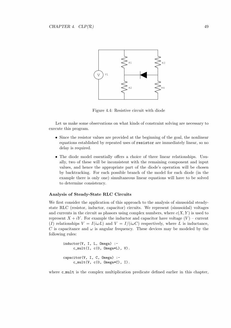
CHAPTER 4. CLP(R) 49
V1
V V1
R1 R3
R4R2
Figure 4.4: Resistive circuit with diode
Let us make some observations on what kinds of constraint solving are necessary toexecute this program.
• Since the resistor values are provided at the beginning of the goal, the nonlinearequations established by repeated uses of resistor are immediately linear, so nodelay is required.
• The diode model essentially offers a choice of three linear relationships. Usu-ally, two of these will be inconsistent with the remaining component and inputvalues, and hence the appropriate part of the diode’s operation will be chosenby backtracking. For each possible branch of the model for each diode (in theexample there is only one) simultaneous linear equations will have to be solvedto determine consistency.
Analysis of Steady-State RLC Circuits
We first consider the application of this approach to the analysis of sinusoidal steady-state RLC (resistor, inductor, capacitor) circuits. We represent (sinusoidal) voltagesand currents in the circuit as phasors using complex numbers, where c(X,Y ) is used torepresent X + iY . For example the inductor and capacitor have voltage (V ) – current(I) relationships V = I(iωL) and V = I/(iωC) respectively, where L is inductance,C is capacitance and ω is angular frequency. These devices may be modeled by thefollowing rules:
inductor(V, I, L, Omega) :-c_mult(I, c(0, Omega*L), V).
capacitor(V, I, C, Omega) :-c_mult(V, c(0, Omega*C), I).
where c mult is the complex multiplication predicate defined earlier in this chapter,

CHAPTER 4. CLP(R) 50
by:
c mult(c(R1, I1), c(R2, I2), c(R3, I3)) :-R3 = R1 * R2 - I1 * I2,I3 = R1 * I2 + R2 * I1.
Let us consider now in more detail how the c mult predicate might be used andwhat kinds of constraints it might establish. We use the italic notation for CLP(R)variables that have known values.
• In general, two nonlinear equations may have to be delayed until further infor-mation is available.
• When the two complex values to be multiplied are available in advance, the twoconstraints can be solved by local propagation, using simple arithmetic evalua-tion. That is, when two complex numbers are multiplied, R1, I1, R2, and I2 areavailable, so the equations can be directed as the independent propagations:
R3 ← R1R2 − I1I2I3 ← R1I2 +R2I1
• When two complex values to be divided are available in advance, two simultaneouslinear equations must be solved locally. That is, for example, when R1, I1, R3,and I3 are all available, it is necessary to solve
R3 = R1R2− I1I2I3 = R1I2 + I1R2
for R2 and I2.
To connect networks of these components together, we have to satisfy the variousconservation laws at the interface of the components. This can be done by ensuringthat:
• all component terminals that are connected together are at the same voltage, and
• for each node, the sum of the currents flowing into the node is zero.
Appendix A.1 contains a general package for solving arbitrary sinusoidal steady-state RLC circuits that incorporates these ideas. The package is run using the predicatecircuit solve with four arguments. They are respectively: the source frequency,circuit representation, the nodes at ground potential and the nodes whose values areto be printed after the analysis. The package can also be used for D.C. analysis bysetting the frequency and imaginary parts of quantities to zero. This is illustrated bythe following goal, which analyzes the circuit of Figure 4.5.

CHAPTER 4. CLP(R) 51
V1 V
R1
R2V1 D1
n1 n2
ground
Figure 4.5: Use of the general package to solve a DC circuit
?- W = 0,Vs = 10,R1 = 100,R2 = 50,circuit_solve(W,
[[voltage_source,v1,c(Vs,0),[n1,ground]],[resistor, r1, R1, [n1, n2]],[resistor, r2, R2, [n2, ground]],[diode, d1, in914, [n2, ground]]],[ground],[n2]).
Output is:
COMPONENT CONNECTIONS TO NODE n2resistor r1: 100 OhmsNode n2 Voltage c(0.60082, 0) Current c(-0.0939918, 0)resistor r2: 50 OhmsNode n2 Voltage c(0.60082, 0) Current c(0.0120164, 0)diode d1: type in914Node n2 Voltage c(0.60082, 0) Current c(0.0819754, 0)
The second example shows a larger RLC circuit (Figure 4.6).
?- W = 100, Vs = 10, Tr1 = 5, Tr2 = 0.2,R1 = 200, R2 = 1000, R3 = 50, R4 = 30,C1 = 0.05, L1 = 0.005,circuit_solve(W,
[[voltage_source, v1, c(Vs,0),[in, ground1]],[resistor, r1, R1, [in, n1]],

CHAPTER 4. CLP(R) 52
V1
R1
TR1
R2
TR2
R3 R4
C1
L1
ground1 ground2 ground3
out
V1
in n1 n2
n3
n4
Figure 4.6: RLC Circuit
[transformer, t1, Tr1,[n1, ground1, n2, ground2]],[resistor, r2, R2, [n2, n3]],[capacitor, c1, C1, [n3, n4]],[resistor, r3, R3, [n4, ground2]],[transformer, t2, Tr2,[n4, ground2, out, ground3]],[resistor, r4, R4, [out, ground3]][inductor, l1, L1, [out, ground3]]],[ground1, ground2, ground3],[out]).
Output is:
COMPONENT CONNECTIONS TO NODE outtransformer t2: ratio of 0.2Node out V c(3.34983e-06, 0.0001984) C c(-0.0003968 8.78204e-08)resistor r4: 30 OhmsNode out V c(3.34983e-06, 0.0001984) C c(1.11661e-07,6.61185e-06)inductor l1: 0.005 HenryNode out V c(3.34983e-06, 0.0001984) C c(0.0003967, -6.69967e-06)
Finally, let us again consider the critical operations that this program’s executiondepends on:
• traversal of the data structures representing the circuits, requiring essentiallysyntactic unification
• solving simultaneous linear equations representing constituent relationships andnetwork relationships
• backtracking to find the right operating mode for components modeled by a piece-wise linear relationship
Transistor Circuits: Analysis and Design
If more realistic applications are to be tackled, transistors must be addressed in someway. While the voltage-current behavior of the transistor is highly nonlinear, it can

CHAPTER 4. CLP(R) 53
be modeled for most practical purposes using piecewise linear techniques. We willillustrate this approach through the analysis and design of amplifier circuits using thebipolar junction transistor. This approach is equally applicable to other types of circuitand other types of transistor.
Typical engineering methods for the design of transistor circuits are iterative andguided by heuristics. This involves estimating key circuit parameters, computing theremaining unknown values, and then making corrections to the original estimates. Theprograms we present use a similar approach. However, we replace iteration by back-tracking.
The design of transistor amplifiers falls into three stages.
1. The basic form of the amplifier is selected (for example: common-base, emitter-follower).
2. The biasing circuitry is designed to ensure that the transistor will operate inits active mode within the expected range of inputs to the circuit. Design re-quirements include insensitivity to transistor parameters such as common-emittercurrent gain, and temperature.
3. The requirements of the small signal operation of the amplifier are satisfied. Theserequirements may include high input resistance, low output resistance and pre-dictable gain.
The package presented in Appendix A.2 provides both simple D.C. analysis forbiasing and digital circuitry, and small signal analysis for transistor amplifiers. Thetransistor is modeled by three modes of operation: active, saturated and cutoff. Foramplifier circuits we are primarily interested in the active mode of operation, while fordigital circuits the saturated and cutoff modes become important. The rules in Figure4.7 give the D.C. properties of an NPN transistor (Figure 4.8) in the three modes.The variables Beta, Vbe and Vcesat are device parameters; Vx and Ix are respectivelyvoltages and currents, where x ranges over b (base), e (emitter), c (collector).
Again this will introduce an element of nondeterminism into the analysis, as thesolution of simultaneous equations (and possibly inequalities) will cause backtrackinguntil a consistent configuration is found.

CHAPTER 4. CLP(R) 54
transistor_dc(active, npn, Beta, Vbe, Vcesat,Vb, Vc, Ve, Ib, Ic, Ie) :-
Vb = Ve + Vbe,Vc >= Vb, Ib >= 0,Ic = Beta*Ib,Ie = Ic + Ib.
transistor_dc(saturated, npn, Beta, Vbe, Vcesat,Vb, Vc, Ve, Ib, Ic, Ie) :-
Vb = Ve + Vbe,Vc = Ve + Vcesat,Ib >= 0, Ic >= 0,Ie = Ic + Ib.
transistor_dc(cutoff, npn, Beta, Vbe, Vcesat,Vb, Vc, Ve, Ib, Ic, Ie) :-
Vb < Ve + Vbe,Ib = 0,Ic = 0,Ie = 0.
Figure 4.7: DC model of NPN transistor
V1
b e
c
Vc
Ve
Vb
Ic
Ie
Ib
Figure 4.8: An NPN type transistor

CHAPTER 4. CLP(R) 55
V1
b e
c
RRB1 C
RB2 RE
100k
50k
5k
3k
cc1
gnd
15VV
Figure 4.9: Biasing Circuit for NPN transistor
With the addition of the previously defined rule for modeling the (D.C.) propertiesof resistors, we are able to analyze some simple circuits. For example the simple biasingcircuit shown in Figure 4.9 may be analyzed using the following goal:
?- resistor(15 - Vb, I1, 100),resistor(-Vb, I2, 50),I1 + I2 = Ib,transistor(State, npn, 100, 0.7, 0.3,
Vb, Vc, Ve, Ib, Ic, Ie),resistor(Ve, Ie, 3),resistor(15 - Vc, Ic, 5).
Notice how the variable State is used here to determine which of the three modesthe transistor must operate in.
The full program in Appendix A.2 is an extension of these rules to allow the D.C.analysis of more general transistor circuits, which may include capacitors and diodes.This program is written to reflect the structure of the problem by defining componentvoltage-current relationships at one level, and component connections, at a higher level,in terms of these voltage/current parameters. The circuit structure is defined by listingthe components and their connections. For example, the following goal again analyzesthe circuit of Figure 4.8.
?- Vcc1 = 15, dc_analysis(Vcc1, _, [[resistor, rb1, 100, [cc1, b]],[resistor, rb2, 50, [gnd, b]],[transistor, t1, [npn,tr1,State], [b,c,e]],[resistor, re, 3, [e,gnd]],[resistor, rc, 5, [c,cc1]]]).

CHAPTER 4. CLP(R) 56
Output is:
State = active
A number of different types of problems can be solved with this package. For ex-ample the following goal does not specify the component values, but instead constrainsthem to lie within certain ranges.
?- Vcc1 = 15, 27 <= R1, R1 <= 100, 5 <= R2, R2 <= 27,dc_analysis(Vcc1, _, [
[resistor, r1, R1, [cc1,b]],[resistor, r2, R2, [gnd,b]],[transistor, t1, [npn,tr1,State], [b,c,e]],[resistor, r3, 3, [e,gnd]],[resistor, r4, 5, [c,cc1]]]).
Output is:
State = activeR1 = 50R2 = 27
In this case, the resistor relationships only become linear when the solving of otherequations results in the currents being determined. Then the resistances can be deter-mined uniquely.
Finally we can re-employ the analysis program as a design program. This canbe achieved by constraining the design parameters, choosing a circuit template, andco-routining the search for suitable components with a circuit analysis – the test andgenerate technique. After a circuit template has been chosen, the circuit analysis rulesare used to set up the appropriate constraints, and then the search for components takesplace. When values are chosen for components, an inappropriate choice will often causethe system of constraints to become unsatisfiable immediately, leading to backtracking(assuming that the determination of unsatisfiability does not rely on the considerationof nonlinear constraints). In this way we avoid an exhaustive search to find componentvalues that satisfy the design constraints. A goal for designing a positive gain transistoramplifier is shown below.
?- Vcc = 15, Stability < 0.5, Gain > 0.5,Inresistance >= 25, Outresistance <= 0.5,full_analysis(Vcc, _, Circuit, _, _, Type, Stability,
Gain, Inresistance, Outresistance).
Output is:
Circuit= [[capacitor, c1, C1, [p1,b]],[resistor, r1, 100, [b,cc1]],[resistor, r2, 100, [b,gnd]],

CHAPTER 4. CLP(R) 57
[transistor, tr, [npn,tr0,active], [b,cc1,e]],[resistor, re, 5, [e,gnd]],[capacitor, c3, C3, [e,out]]]
Type = emitter_followerStability = 0.13Gain = 0.99Inresistance = 45.51Outresistance = 0.47
The approach of co-routining constraint satisfaction with the search for componentsresults in a search space pruning of two orders of magnitude and the total time takenis reduced by more than an order of magnitude over the exhaustive search approach.The execution of the analysis program when used in this way is completely different.The circuit template is chosen first, and then all of the various constraints are imposedwithout any actual component values having been established. This means that a largesolved form of linear equations and inequalities, as well as delayed linear inequalities,will be established. Only when all this has been done will the component values beguessed at exhaustively, resulting in the partial simplification of solved constraintsand the awakening of delayed constraints, which will frequently have to be undonewhen an incorrect guess is made. As this goal will certainly exercise our claims aboutthe kinds of constraints arising in constraint solving, and the subsequent decisionsabout implementation, we will naturally return to it in the empirical study of CLP(R)programs.
4.3.2 Digital Signal Flow
We concentrate in this subsection on the simulation of linear shift-invariant digitalsystems with time as the independent variable [134]. We represent digital systems interms of linear signal-flow graphs. A signal flow graph is a collection of nodes anddirected branchers. Associated with each node is a variable, which represents thesignal value at that node. Source nodes have their signal value determined at eachstage by some input signal. Branches are either multiplier branches or delay branches.A multiplier branch multiplies the signal at its input end by its labeling coefficient togive its output; a delay branch has as output its input at the previous time step. Thesignals at each node in the signal flow graph are such that the signals in any outgoingbranches are equal to the sum of the signals in the incoming branches (the summingconstraint). As an example, consider the digital filter described in Figure 4.10.
We simulate the signal-flow graph by computing the signal values at the nodesat successive time steps, starting from some given initial values. This is achieved bycollecting branch equations and summing constraints for each node. This, along withthe input signal values to the source nodes, is sufficient to determine the signal valuesat each node for each time step.
The signal-flow graph simulator appearing in Appendix A.3 is called using thepredicate flow with a description of the graph as the first argument and the name ofthe node where the value is to be printed as the second argument. The following goaldescribes the low pass filter of Figure 4.10.

CHAPTER 4. CLP(R) 58
delayinput
output
n1 n2 n5n3 n4delay delay delay
n6
0.20.2
0.20.20.2
Figure 4.10: High frequency filter
1
0
-1
1
0
-1
Figure 4.11: Input and output for filter
?- flow([[source, in, n1],[delay, n1, n2], [delay, n2, n3],[delay, n3, n4], [delay, n4, n5],[coeff(0.2), n1, n6], [coeff(0.2), n2, n6],[coeff(0.2), n3, n6], [coeff(0.2), n4, n6],[coeff(0.2), n5, n6]],n6).
Figure 4.11 shows the output from the program in graphical form corresponding to theaccompanying square wave input.
Again we should consider what kind of constraint solving is needed in this applica-tion. Much of it involves local propagation, as specific inputs are given, and just needto be propagated through the nodes of the signal flow graph. However, consider whathappens when the graph involves a loop. We can reason about the way constraints aresolved analogously to how the signal flows through the graph. So if the loop contains adelay branch, The node that obtains the feedback value depends only on earlier values,

CHAPTER 4. CLP(R) 59
ph ah
bh
qh
O
B
Q
P A
uO(ap+ bq)apbq
=uA
a(a+ p)+
uB
b(b+ q)+
uP
p(p+ a)+
uQ
q(q + b)
Figure 4.12: Liebmann’s 5-point approximation to Laplace’s equation
so local propagation is still sufficient. However, if there is no delay element in theloop, that node’s value depends partly on itself. Hence simultaneous equations mustbe solved.
4.3.3 Electro-Magnetic Field Analysis
Often it is undesirable or impractical to analyze electrical systems in terms oflumped circuit components. In many cases an analysis using electro-magnetic fieldtheory is required, typically involving the solution of partial differential equations sub-ject to some boundary or initial conditions. A simple way to solve these problems isto use a finite difference approximation. We will consider the five-point approximationto Laplace’s equation known as Liebmann’s method described in Figure 4.12, whichcan be used to solve Dirichlet, Neumann and mixed boundary value problems. Thefinite difference equations are the leaf constraints — they apply to a neighborhood ofpoints. The complete finite difference problem is a parent constraint arising from theoverlapping of these neighborhoods.
Figure 4.13 shows a simple program to solve the Dirichlet problem for Laplace’sequation in two dimensions, with a sample query and output. The region of interest isrepresented as a matrix (list of lists) of anonymous variables, with constants at the edgespecifying the boundary values. Constraints (finite difference equations) are collected

CHAPTER 4. CLP(R) 60
Program:
laplace([_,_]).laplace([H1,H2,H3|T]):-
laplace_vec(H1,H2,H3),laplace([H2,H3|T]).
laplace_vec([_,_],[_,_],[_,_]).laplace_vec([TL,T,TR|T1],[ML,M,MR|T2],[BL,B,BR|T3]):-
B + T + ML + MR - 4*M = 0,laplace_vec([T,TR|T1],[M,MR|T2],[B,BR|T3]).
Sample goal:
?- laplace([[0, 0, 0, 0, 0, 0, 0],[100, _, _, _, _, _, 100],[100, _, _, _, _, _, 100],[100, _, _, _, _, _, 100],[100, _, _, _, _, _, 100],[100, _, _, _, _, _, 100],[100, 100, 100, 100, 100, 100, 100]]).
Output:
[[0, 0, 0, 0, 0, 0, 0],[100, 53.1, 37.1, 33.1, 37.1, 53.1, 100],[100, 75.4, 62.1, 58.1, 62.1, 75.4, 100],[100, 86.5, 77.9, 75.0, 77.9, 86.5, 100],[100, 92.8, 87.9, 86.2, 87.9, 92.8, 100],[100, 96.9, 94.6, 93.9, 94.6, 96.9, 100],[100, 100, 100, 100, 100, 100, 100]]
Figure 4.13: Solving Laplace’s equation

CHAPTER 4. CLP(R) 61
at each point of the matrix by “sliding” a “window” of 9 points across the matrix andreferring only to the variables in that window. Simultaneous linear equations must besolved at run time.
4.4 Survey of Other Applications
Since the first prototype implementation of CLP(R) became generally available in 1987,a number of other applications have been explored in considerable detail by variousresearchers. In fact, some of these projects were inspired by early versions of the workdescribed above. Some of the more significant projects are briefly outlined here. Mostuse versions of the system based on material in Part III of this thesis.
• Genetic Restriction Site MappingThe restriction site mapping problem is to reconstruct the placement of certainDNA subsequences on a molecule corresponding to a given enzyme given data onthe digest fragments produced when the molecule is treated with that enzyme.In [192], Yap describes a methodology for solving this problem using CLP(R)programs. The problem is of tremendous practical importance, and is compu-tationally intractable in general. The programs involve reasoning with linearequations and inequalities on real-valued variables.
• Civil EngineeringIn [102], Lakmazaheri and Rasdorf described the use of CLP(R) for the analysisand partial synthesis of truss structures. Their program consists of only sixteenrules, and deals with general two-dimensional truss structures with pin and rollersupports, concentrated loads, and truss elements with uniform cross section. Theprogram uses constraints to describe the physical behavior of structural compo-nents. Considerable use is made of symbolic answer constraints. The constraintstend to be linear and nonlinear equations. In addition to checking the validity oftruss and support components, the program can be used to generate their spatialconfigurations.
• Options Trading AnalysisOTAS [104, 78, 79] is a system for designing stock option investment portfo-lios. Linear equations and inequalities, as well as nonlinears were used to modelexpected payoffs. Unsatisfiable linear inequalities were also used. Additionally,considerable use was made of CLP(R)’s output constraints.
In [74], Homiak described the use of CLP(R) for solving partial differential equa-tions arising in the domain of options valuation. Problems are described usinga symbolic input language from which CLP(R) constraints are generated. Theexamples in the document include cases where the grid has up to 6000 elements.The PDEs are solved using various finite difference techniques, and thus this(large) piece of software is a natural generalization of the tiny program shownabove for solving Laplace’s equation.

CHAPTER 4. CLP(R) 62
• Configuration Design for Mechanical SystemsIn [173], Sthanusubramonian discusses the use of CLP(R) to design gear boxes,given physical constraints on the size and layout of a gearbox, as well as functionalconstraints on the outputs. The arithmetic constraints are mostly nonlinear,and hence CLP(R) is mostly used to collect and maintain systems of nonlinearconstraints.
• Generation of Test Data for Protocol VerificationIn Mockingbird [57], CLP(R) is used to implement grammars that model com-munications protocols. By running the programs “in reverse”, these grammarsare used to generate sample messages, and additional constraints are used to tunethe type of messages produced. The constraints are typically linear equalities andinequalities, and the values considered are usually integers.
• Temporal ReasoningIn [135], Ostroff describes the use of CLP(R) as a computational logic for mod-eling, simulating and verifying real-time discrete event processes. Constraintsolving is used to avoid the combinatorial explosion that results from the stateenumeration normally used for such verification. The constraints are mostly sim-ple linear equations and inequalities, and the intended domain of the modeling isthat of integers.
In [5, 6], Amon and Borriello describe the use of CLP(R) for verifying that behav-ioral constraints on classes of asynchronous circuits are satisfied. The programsmake use of linear equations and inequalities, and use answer constraints to relatetiming delays, making tradeoffs apparent.
• Interactive Tutoring for Music TheoryIn [182], Tobias discusses the Harmony Intelligent Tutoring System, with particu-lar emphasis on the Harmony Expert module, which is implemented in CLP(R).The Harmony Expert involves a complex set of inference rules incorporating lin-ear equations and inequalities on variables ranging over a finite, convex set ofintegers. The methodology makes use of non-trivial output constraints as well.
• Modeling Concurrent Execution of ProgramsIn [116], Mercouroff and Weitzman discuss the use of Prolog III and CLP(R) tomodel the execution times of a class of recursive parallel programs. The CLP pro-grams involve linear equations and inequalities, and provide analytical solutionsto the problem of determining the execution time of the corresponding parallelprogram. Rational numbers are the ideal domain.
4.5 Empirics
Now that we have studied programming methodology and typical programs from astatic viewpoint, we need to understand how programs behave at run time. Thuswe provide measurements for the runtime behavior of a number of CLP(R) programs.
CHAPTER 4. CLP(R) 63
Some of the results were foreshadowed by the study of Yap [191], using an early CLP(R)interpreter. The measurements were obtained by instrumenting Version 1.1 of the IBMCLP(R) compiler, many aspects of which are described in some detail later in thisthesis. This analysis is somewhat circular, since the results are being used to justifydecisions made about the language design and implementation, and are obtained froma system incorporating those decisions, using programs written by programmers oftenaware of those decisions, for that implementation. While this means that the figuresshould be taken with a grain of salt, they are still clearly of great value, since theydemonstrate certain characteristics rather decisively.
The statistics are presented on a per-goal-per-program basis for a representativesuite of programs. Some of the parameters will not make very much sense at this pointin the exposition because they rest heavily on subsequent implementation chapters.Below we attempt to give some intuition as to what they correspond to in terms of theprograms. They are in four broad categories:
• ResolutionsThis indicates the overall amount of computation and search.
Call The number of subgoals reduced. Shallow backtracking does not addto this total, but deep backtracking does.
Fail Number of failures of any kind, thus a measure of amount ofbacktracking.
• Disagreement PairsThese are essentially equations arising from attempting to resolve a subgoal.
Top Number of top level equations. Each attempt to reduce a subgoal withan n-ary predicate results in n such equations. Thus backtracking addsto this total.
Rec This is the total number of equations. One equation of the above kindcan result in several equation, say when subterms of uninterpretedfunctors are equated. We call these equations disagreement pairs.
%PP The percentage of disagreement pairs that equate two solver variables.%VP The percentage of disagreement pairs that equate a solver variable and
a free variable.%VV The percentage of disagreement pairs that equate two free variables.

CHAPTER 4. CLP(R) 64
• Arithmetic EquationsSummarizes the amount of arithmetic dynamically occurring.
EQ Number of explicit linear arithmetic equations. This is loosely relatedto the number of such equations occurring in the program, since thecompiler performs transformations on constraints.
Num Number of real (floating point) numbers explicitly assigned to solvervariables.
Calls Number of equations actually passed to the linear equation solver.New Number of the above equations that did not really require solving,
since they included a new variable.Ground Number of the above that immediately give a ground value to the new
variable.Par Number of equations passed to the solver that resulted in a simplifying
substitution. Essentially these are the rest of the equations passed tothe solver.
• InequalitiesThis is to capture the number of explicit linear inequalities arising.
GT Number of strict linear inequalities encountered.GE Number of non-strict linear inequalities encountered.ICalls Number of inequalities and equations passed to the inequality solver.
There is no simple relationship between this parameter and the othersabove. The inequalities passed result either from the GT or GE pa-rameters, but the equalities can result either from EQ instances of thePar kind, or from Num instances or PP type disagreement pairs. Thiswill be explained in more detail when discussing the implementationof CLP(R).
The results are summarized in four tables. The first two, in Figures 4.14 and4.15, are for a set of simple example programs. Some of these, like Mortgage or SMMactually perform a lot of computation, but they are typically small programs written toillustrate various aspects of the use or performance of CLP(R). The third and fourthtables, in Figures 4.16 and 4.17, contain results from more substantial programs. Mostof these were also written to illustrate the use of CLP(R), but are often quite large andcomplicated, are more concerned with the actual applications, and in some cases werewritten by programmers who were not involved with any implementation of CLP(R).Many of the programs have already been discussed. We give some relevant detailsabout the programs and queries.
• FibThe Fibonacci program for early in this chapter. The first goal uses it to computeF14, and the second goal computes the inverse function.
• MortgageThis is a form of the mortgage program (similar to that shown in this chapter)
CHAPTER 4. CLP(R) 65
given in Chapter 10. The four queries given there are used, as they represent fourdifferent uses of the program.
• OptionThis is a program for reasoning about algebraic combinations of stock optiontransactions, described in [104]. The two goals obtain all solutions to queriesabout combinations of put and call options.
• LadderA simple program for reasoning about resistive circuits – specifically various volt-age dividers, ladder networks and bridges. Used for teaching CLP(R) program-ming at the University of Washington, and written by Alan Borning. The variousgoals analyze various circuits of this kind.
• SMMThis is the SEND+MORE=MONEY puzzle of Figure 4.2.
• LaplaceThis is the program shown in this chapter for solving Laplace’s equation, with alarger goal grid.
• CriticalThis is a program written by Roland Yap for critical path analysis. Constraintsare used to avoid the multiple passes through the graph. The goals analyze varioussizes of graphs.
• DiscreteThis program, written by Jonathan Ostroff and Jeff Klein, is described in [135]. Itreasons about discrete event processes, and the query used to obtain these resultsis the filterpath(trainGate) query described in the paper.
• VerifyThis program described above, was written by Amon and Borriello [5, 6] forverifying asynchronous circuits. Some of the goals run for a very long time.These are examples from their various papers.
• DNAThis is the program for genetic restriction site mapping written by Yap [192],using various examples similar to those in that paper.
• EEThis is a program similar to that described earlier in this chapter and in [69]for analysis and synthesis of electrical circuits with diodes and transistors. Thefirst goal determines the activation state of a transistor in a circuit, the secondanalyzes a NAND gate, the third designs an amplifier using the test-and-generatemethodology, and the fourth obtains the same design with much more work, usingexhaustive search.
CHAPTER 4. CLP(R) 66
• GearsThis is a gear-train design program, written by Devika Subramanian and Cheuk-San Wang at Cornell University. The query is the biggest synthesis query madeavailable, searching only for the first solution.
While we will draw heavily on these results in subsequent chapters, it is appropriateto make a few general observations at this stage.
1. The large numbers of VV and VP cases in unification in many programs showthe importance of the extended unification algorithm in Chapter 7.
2. The “New” category of arithmetic equations shows that many linear equalitiesencountered are a priori clearly consistent with the set of collected constraints.
3. The “Ground” category of arithmetic equations demonstrates that a substantialfraction represent forward propagation steps.
4. The analysis of inequalities shows that in many programs a substantial fractionof inequalities are simple tests. The ratio of the number of arithmetic constraintsto the number of disagreement pairs varies substantially between programs, butgenerally is very small.
5. All of the programs make use of non-trivial arithmetic constraint solving, butmost of them do so sparingly.

CHAPTER 4. CLP(R) 67
Resolutions Disagreement PairsProgram Query Call Fail Top Rec %PP %VP %VV
Fib Fw 611 0 2438 2438 75 25 0Bw 1505 999 8155 8155 70 30 0
Mortgage 1 361 1 1805 1805 0 80 202 361 1 1805 1805 0 100 03 361 1 1805 1805 0 100 04 358 3 1800 1800 0 100 0
Option 1 33 15 206 206 0 63 272 105 49 690 690 0 62 30
Ladder 1 15 4 47 117 11 26 32 14 3 42 99 11 25 33 20 7 73 188 11 26 34 19 6 68 170 11 26 35 21 9 86 227 11 27 36 20 8 81 209 11 27 37 213 101 930 2254 12 27 4
SMM 1262 1247 6580 11202 10 33 0Laplace 113 90 514 2582 0 29 6Critical 1 124 80 595 1433 0 15 16
2 511 446 2882 7219 0 13 163 382 339 2139 5310 0 14 15
Discrete 1 1079 547 1891 3439 0 28 0
Figure 4.14: Small Programs: Resolution and Unification

CHAPTER 4. CLP(R) 68
Arithmetic Equations InequalitiesProgram Query EQ Num Calls New Ground Par GT GE ICalls
Fib Fw 1827 1221 4627 3049 1218 1218 609 0 0Bw 5559 3206 12848 8766 3071 4028 2475 0 39
Mortgage 1 719 5 1083 1083 719 0 360 359 02 719 5 1083 1082 359 1 360 359 13 719 3 1081 1080 359 1 361 360 3624 716 6 1081 1075 356 6 357 359 365
Option 1 15 28 66 62 6 4 14 32 372 50 105 235 235 25 0 48 108 126
Ladder 1 12 10 35 23 0 12 0 0 02 11 8 30 20 0 10 0 0 03 19 15 56 36 0 20 0 0 04 18 13 51 33 0 18 0 0 05 24 14 65 41 0 24 0 0 06 23 12 60 38 0 22 0 0 07 267 111 686 438 19 248 19 0 0
SMM 4 63 276 64 0 212 0 26 236Laplace 81 40 122 113 0 9 0 0 0Critical 1 28 7 40 37 24 3 2 0 0
2 105 21 151 133 81 18 10 0 03 77 16 110 101 66 9 7 0 0
Discrete 1 22 362 194 171 22 23 0 30 31
Figure 4.15: Small Programs: Arithmetic
Resolutions Disagreement PairsProgram Query Call Fail Top Rec %PP %VP %VV
Verify 1 26941 26404 108466 226915 0 5 12 132189 134280 543085 1078951 0 2 03 6003326 6116029 24589775 49470767 0 1 04 5036771 5148358 20702284 41478978 0 1 05 6003267 6116029 24589775 49470767 0 1 0
DNA 1 99 68 549 1181 5 37 42 10445 8939 58565 136715 6 41 2
EE 1 109 106 990 1733 1 8 232 137 131 1248 2255 0 10 213 1623 1978 17941 27605 1 9 234 101583 126118 1062863 1745129 0 7 25
Gears 39161 26261 157762 659201 6 25 6
Figure 4.16: Large Programs: Resolution and Unification

CHAPTER 4. CLP(R) 69
Arithmetic Equations InequalitiesProgram Query EQ Num Calls New Ground Par GT GE ICalls
Verify 1 51 523 586 574 38 12 714 86 482 175 1030 1217 1205 157 12 1417 482 493 1218 8292 9511 9484 1102 27 9986 2276 2794 1254 6929 8184 8167 1168 17 8812 2874 2575 1218 8290 9509 9482 1102 27 9986 2276 281
DNA 1 64 27 147 105 43 42 35 26 872 6969 1030 11350 8029 5311 3321 5383 1035 8896
EE 1 24 50 83 76 3 7 0 2 42 37 59 103 93 7 10 2 4 73 389 974 2586 1400 42 1186 2 20 3644 24215 18971 53085 45353 2436 7732 2 1472 3617
Gears 88650 53558 242001 230115 77805 11846 3419 0 0
Figure 4.17: Large Programs: Arithmetic

Chapter 5
λProlog and Elf
The idea of a language based on solving equations between simply-typed λ-expressionsemerged from the desire to use λ-abstraction as a means of representing data ratherthan defining functions. The first language based on the idea was λProlog [121]. Inthis chapter we will discuss the closely related language Elf [139], although much of thematerial is equally applicable to λProlog. The chapter will begin with an introductionto the languages, and will continue with a discussion of programming methodology andempirical observations.
5.1 The Domain
The core domain of Elf is the set of βηα-equivalence classes of λ-expressions withdependent types, where application is the only operation and equality is the only re-lation. The terms are thus typed lambda expressions with constructors (functors andconstants) and existentially quantified variables. A term free of existential variablescan be considered ground. As we shall see later, full Elf actually involves constraintson expressions from the λ-calculus with dependent types. For an introduction to thesimply-typed λ-calculus, the reader should consult [143]. Here we will give only a briefoverview by way of example. The equalities
λx : τ. x = λy : τ. y
λx : τ. fa = λx : τ. f((λy : τ. y)a)
hold, whileλx : τ. λy : τ. x = λy : τ. λx : τ. x
does not. Now consider equalities involving terms with existentially quantified variables.
∃M : τ. λx : τ. M x = λx : τ. x
is satisfiable, with M = λx : τ. x being one solution. This is maximally general, andalso unique, modulo βηα-equivalence. On the other hand, some constraints can have
70

CHAPTER 5. λPROLOG AND ELF 71
more than one maximally general solution. For example,
∃M : τ → τ. faa = Ma
has the solutions
M = λx : τ. fxxλx : τ. fxaλx : τ. faxλx : τ. faa
of which no two are βηα-convertible. In fact, sometimes there are infinitely manymaximally general solutions. Consider
∃M : τ → τ. M(fa) = f(Ma),
which has the solutions
M = λx : τ. fnx, n ∈ 0, 1, 2, · · ·.One major design issue related to these languages comes from the fact that con-
straint satisfiability is undecidable. It is semi-decidable, but the pre-unification algo-rithm of Huet [76], and Elliot’s extension to dependent types [50], as demonstratedabove, involve backtracking through solutions to individual equations. Details of theseissues will be discussed in Chapter 11.
There are three prevailing approaches to dealing with this problem:
• Tolerate the inefficiencyIt may be that some kinds of programs actually can benefit from the full generality,although this has not been argued convincingly.
• Restrict the language to a fragment with decidable constraintsIn [119], Miller presents a language Lλ, described below, which is syntacticallyrestricted such that the hard cases of unification do not occur. It is claimed thatthis subset is satisfactory for most examples. However, programming becomesmore difficult for certain examples, as idioms that can be expressed directly inthe full language here have to be coded up explicitly. This can also result in aloss of efficiency, as will be demonstrated in Section 5.6.
• Introduce delay for the constraints that cause inefficiencyMany Elf programs actually conform to the restrictions of Lλ, and it turns outthat many programs that do not conform to the syntax of Lλ still do not involvethe difficult case of unification dynamically. Furthermore, it has been argued byPfenning [139] that many of the remaining programs could avoid the difficult caseif certain constraints were deferred until they were sufficiently instantiated to fallinto an easier case. This is directly analogous to the case for delay of nonlinearsin CLP(R), and will be examined more closely here and also in Chapter 11.

CHAPTER 5. λPROLOG AND ELF 72
It should be noted that, while Elf is certainly a CLP language in essence, it departsfrom the pure CLP scheme in a number of unusual ways.
• it is strongly typed;
• embedded implication, first described by Miller in [118], is used to modify theprogram with temporary assumptions, as a central programming technique;
• universal quantification is provided, and is central to programming technique, asit essentially provides a new constant different from all other constants occurringso far;
• programs can manipulate proof objects, in a way that is kept under control bythe type system.
The language λProlog is closely related to Elf, many of the same design, program-ming and implementation observations apply, and it is more widely used than Elf.Hence, it is useful to consider how the two languages differ. λProlog has no ability toreason about proofs of goals. However, it allows polymorphic constructors and predi-cates to be defined, and it also allows predicate variables. That is, predicate symbolsare in many respects treated as constructors.
Finally, Lλ [119] is a syntactically restricted version of Lλ, with a correspondingrestriction of LF [140] for Elf, where variables that are universally quantified at the toplevel of a clause can only be applied to a set of distinct bound variables. As mentionedbefore, and discussed fully in Chapter 11, this is intended to avoid the hard case ofsolving constraints.
5.2 The Languages
To introduce Elf, let us consider in Figure 5.1 an example that is essentially a Prologprogram. It converts propositional formulae to negation normal form. This is verystraightforward, and can be directly translated to Prolog.
First, bool is declared as the type of boolean truth values, and var as the typeof propositional variables. Then the constructors not, and and or are the usual log-ical connectives. Three sample propositional variables v1 to v3 are defined, and theconstructor prop turns a propositional variable into a boolean proposition. The pro-gram consists of one relation negn, which is first declared as a relation between twobooleans. The first rule defining negn, named t nn, eliminates double negation. Thenext two rules t na and t no flip conjunction and disjunction while carrying over anegation. The two base cases (for termination) are t v and t nv. Finally, t o and t apass trough conjunction and disjunction without changing them.

CHAPTER 5. λPROLOG AND ELF 73
bool : type.var : type.
not : b -> b.and : b -> b -> b.or : b -> b -> b.
v1 : var.v2 : var.v3 : var.prop : var -> bool.
negn : bool -> bool -> type.
t_nn : negn (not (not X)) Y<- negn X Y.
t_na : negn (not (and X Y)) (or X1 Y1)<- negn (not X) X1<- negn (not Y) Y1.
t_no : negn (not (or X Y)) (and X1 Y1)<- negn (not X) X1<- negn (not Y) Y1.
t_v : negn (prop X) (prop X).t_nv : negn (not (prop X)) (not (prop X)).t_a : negn (and X Y) (and X1 Y1)
<- negn X X1<- negn Y Y1.
t_o : negn (or X Y) (or X1 Y1)<- negn X X1<- negn Y Y1.
Figure 5.1: Elf program to convert propositional formula to negation normal form

CHAPTER 5. λPROLOG AND ELF 74
As an example query, consider
?- negn (not (and (or (not (prop v1)) (prop v2))(or (prop v3) (not (prop v1))))) X.
which obtains the answer
X = or (and (prop v1) (not (prop v2)))(and (not (prop v3)) (prop v1))
with proof object
t_na (t_no (t_nn t_v) t_nv) (t_no t_nv (t_nn t_v)).
Proof objects will be discussed in more detail in Section 5.4. Essentially, a proofobject is a term constructed from constants declared in an Elf signature, or equivalentlythe names of Elf rules. It represents a record of how the rules of a program were usedto solve a particular query.
Now we can discuss Elf somewhat more systematically. The basic building blockof an Elf program is a signature, that is, a sequence of constant declarations. Some ofthese declarations have the character of declarations for data constructors (functors) orpredicates, while others have the character of declarations of inference rules or clauses.In principle, each declaration could be given all of those interpretations, but in practicefew are meaningful.
This unusual way to view a program stems from the origin of Elf as a computationalview of the Edinburgh Logical Framework (LF) [65], which is type-theoretic. Thisrelationship is justified by the Curry-Howard isomorphism, and Elf is described in thatway in [138].
For a tutorial introduction to Elf, see [117]. Here we give only a brief overview. Thefirst kind of declaration is that of a constant type or type family. Types and type familiesare classified by kinds, the simplest of which is type. Data constructors are declaredusing decl, type and atom. Data is represented using objects. The dependent functiontype, var : type type, is elsewhere often written as Πvar : type. type. Juxtapo-sition is left-associative. The square brackets denote λ-abstraction, and [var : type]obj is more traditionally written as λvar : type. obj . We adopt the shorthand [ var ]and var for those cases of abstraction or quantification where we want Elf typereconstruction to fill in the omitted types. The scope of the abstraction [...] andquantification ... extends to the end of the declaration or enclosing parentheses. Wesummarize the syntax of Elf in Figure 5.2.
In Elf, predicates manifest themselves as type families and thus a type family decla-ration can be interpreted as a predicate declaration. When defining rules we often usethe more conspicuous left-pointing arrow. One should bear in mind that this has nosemantic significance, and A <- B and B -> A are parsed to the same internal repre-sentation. The backwards arrow is left associative and a Prolog rule p :- q, r. wouldbe represented via the type p <- q <- r.
The variable name convention of Elf is much like that of Prolog. Any token begin-ning with an upper case letter is automatically a variable, and if an explicit quantifier is
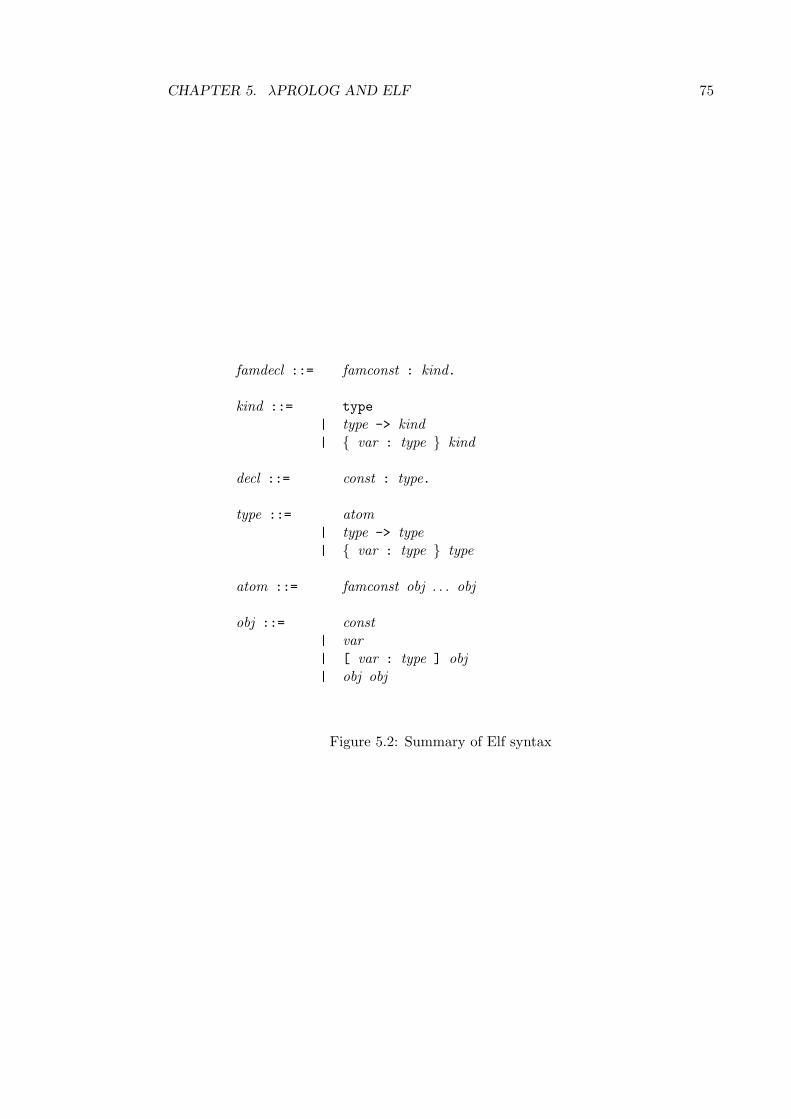
CHAPTER 5. λPROLOG AND ELF 75
famdecl ::= famconst : kind.
kind ::= type| type -> kind| var : type kind
decl ::= const : type.
type ::= atom| type -> type| var : type type
atom ::= famconst obj . . . obj
obj ::= const| var| [ var : type ] obj| obj obj
Figure 5.2: Summary of Elf syntax

CHAPTER 5. λPROLOG AND ELF 76
not provided, one will be added by type reconstruction. Additionally, variables that areexplicitly quantified need not start with an upper case letter. We follow the conventionthat bound variables that will become logic variables (and thus subject to instantiation)during execution of a query are written in uppercase and bound variables that becomeparameters (and thus act like constants to unification) are written in lowercase.
In Elf, unlike Prolog, an underscore character does not denote an anonymous univer-sally quantified variable, although it can sometimes be used for this purpose. Instead,it describes an existentially quantified anonymous variable, and type reconstruction isat liberty to replace an underscore with any term, depending on the available typeinformation. Thus xB and x: B are fully equivalent. In Prolog, since no variablesare ever instantiated during parsing, this distinction does not arise.
Queries to the Elf interpreter consist of a type, possibly with free variables, whichact as logic variables. The goal is to find a term of the given type. In the most commoninterpretation, this term represents a deduction of the judgment that is represented bythe type. During the solution of a goal, the free variables in the query are instantiatedas necessary, as in Prolog. As will be described in more detail later, the names of rulesare used as constructors in assembling deductions.
The operational model of Elf is superficially much like that of Prolog and λProlog. Acomputation rule similar to Prolog’s left-right atom selection rule is employed. Whenusing a rule, the subgoals will be solved “inside-out”. For example, resolving thegoal ?- p. with the rule c : p <- q <- r will first solve subgoal q and then r.Unification is modulo βηα-convertibility, where certain equations are postponed asconstraints. A goal of the form A -> B is solved by adding A to the set of rules availablefor goal reduction. The third form (universal quantification) is solved by replacing theuniversally quantified variable with a new constant.
One complication is that rules and types in Elf are essentially indistinguishable.In fact, the only desired distinction is that of operational behavior. For this reason,the Elf module system [66] allows type families to be defined as either open or closed.Rules defining a closed type family are used to solve goals by search. This distinctionis described in more detail in [139]1.
5.3 Higher-Order Abstract Syntax
Most of the important application areas for Elf are natural extensions of applicationsof λProlog. The major application of λProlog is meta-programming, where the ob-ject language is typically either a programming language or a logic. This is becauseλProlog’s simply-typed λ-expressions enable the use of a meta-programming techniqueknown as higher-order abstract syntax. This approach was inspired by Church [23],Martin-Lof [131] and Huet & Lang [77]. A λ-calculus-based meta-language is used torepresent expressions of the object language. This enables variable binding and scopingin the object language to be represented with the help of λ-abstraction in the meta-
1In more recent work towards a module system for Elf [66] open declarations are called static andclosed declarations are called dynamic according to their role in proof search.

CHAPTER 5. λPROLOG AND ELF 77
language. This, in turn, enables substitution and variable occurrence restrictions to beimplemented using β-reduction in the meta-language, which avoids, for example, therequirement to perform explicit α-conversion to prevent capture of bound variables.
To illustrate these ideas, let us extend the above program to the first-order predicatecalculus. The additional code below introduces the type d for the domain of quantifiedvariables, and a sample predicate symbol p. The interesting constructors are existsand forall, which use abstraction to represent quantifiers. That is, for some formulaΦ, ∀xΦ(x) is represented by ∀(λx.φ(x)), etc. The rules t E and t A simply pass throughthe quantifiers. Note how applying an abstraction to a universally quantified variable isused to descend through the body of the abstraction, and to reconstruct an abstractionfrom the result. The same technique is used in t nE and t nA, except that the quantifiersare flipped because of the descending negation.
dom : type.p : dom -> var.
exists : (dom -> bool) -> bool.forall : (dom -> bool) -> bool.
t_nE : negn (not (exists X)) (forall X1)<- y : dom negn (not (X y)) (X1 y).
t_nA : negn (not (all X)) (exists X1)<- y : dom negn (not (X y)) (X1 y).
t_E : negn (exists X) (exists X1)<- y : dom negn (X y) (X1 y).
t_A : negn (forall X) (forall X1)<- y : dom negn (X y) (X1 y).
As an example query, consider
?- negn (not (exists ([x] (not (prop (p x)))))) X.
has the execution trace
[Solving goal negn (not (exists ([x:dom] not (prop (p x))))) ?X207Resolved with clause t_nESolving goal y:dom negn (not (not (prop (p y)))) (?X1230 y)Introducing new parameter !y232[Solving goal negn (not (not (prop (p !y232)))) (?X1230 !y232)Resolved with clause t_nn[Solving goal negn (prop (p !y232)) (?X1230 !y232)Resolved with clause t_v
which obtains the answer
X = all ([y:dom] prop (p y))

CHAPTER 5. λPROLOG AND ELF 78
with proof object
t_nE ([y:dom] t_nn t_v).
Using λProlog for higher order abstract syntax was described by Pfenning andElliott in [141]. With this technique, λProlog has been used as an implementationlanguage for type inference [137], meta-interpretation [61] and theorem proving [52].These techniques are readily applicable when programming in Elf. We illustrate thetechniques here with parts of the Elf type inference and evaluation code for Mini-ML, asdescribed in [117]. Mini-ML is a small functional language based on a simply typed λ-calculus with polymorphism, products, conditionals, and recursive function definitions.We use the example of application, λ abstraction and polymorphic Älet. The relevantconcrete syntax is as follows.
e ::=...
| lambda x . e| e1 e2| let x = e1 in e2
...
τ ::=...
| τ -> τ...
The three relevant types rules are
of lamΠ , x : τ1 ` e ∈ τ2
Π ` lambda x . e ∈ τ1 -> τ2
of appΠ ` e1 ∈ τ2 -> τ1 Π ` e2 ∈ τ2
Π ` e1 e2 ∈ τ1
of letΠ ` e1 ∈ τ1 Π ` [ e1 / x ] e2 ∈ τ2
Π ` let x = e1 in e2 ∈ τ2
and the relevant evaluation rules are
eval lam ` lambda x . e ⇒ lambda x . e
eval app lam` e1 ⇒ (lambda x . e′1) ` e2 ⇒ α2 ` [ α2 / x ] e′1 ⇒ α
` e1 e2 ⇒ α
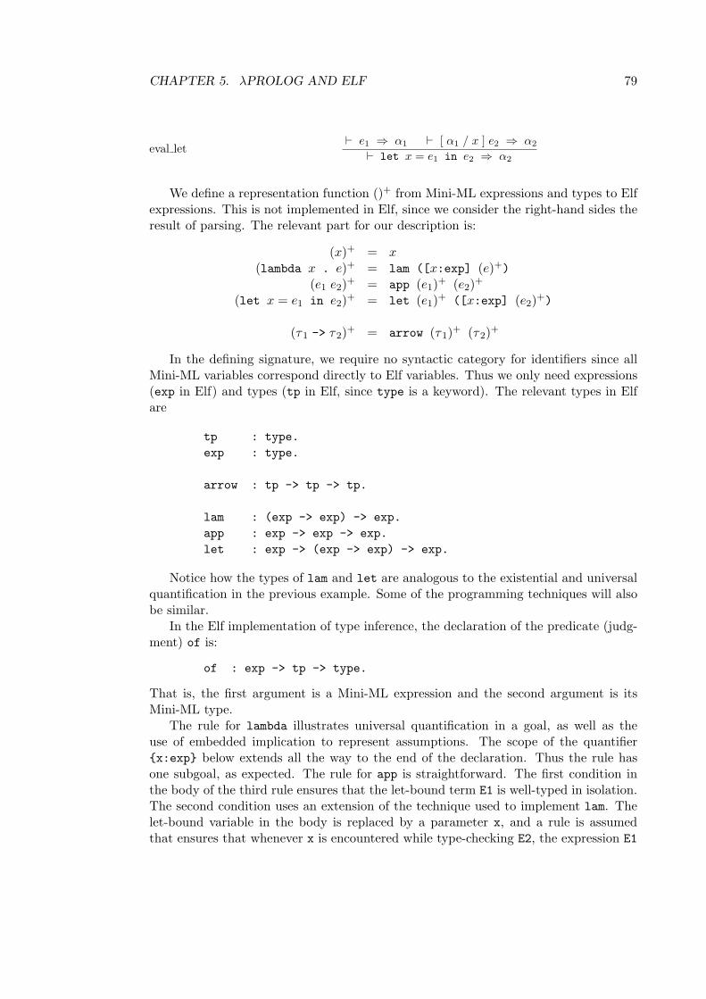
CHAPTER 5. λPROLOG AND ELF 79
eval let` e1 ⇒ α1 ` [ α1 / x ] e2 ⇒ α2
` let x = e1 in e2 ⇒ α2
We define a representation function ()+ from Mini-ML expressions and types to Elfexpressions. This is not implemented in Elf, since we consider the right-hand sides theresult of parsing. The relevant part for our description is:
(x)+ = x(lambda x . e)+ = lam ([x:exp] (e)+)
(e1 e2)+ = app (e1)+ (e2)+
(let x = e1 in e2)+ = let (e1)+ ([x:exp] (e2)+)
(τ1 -> τ2)+ = arrow (τ1)+ (τ2)+
In the defining signature, we require no syntactic category for identifiers since allMini-ML variables correspond directly to Elf variables. Thus we only need expressions(exp in Elf) and types (tp in Elf, since type is a keyword). The relevant types in Elfare
tp : type.exp : type.
arrow : tp -> tp -> tp.
lam : (exp -> exp) -> exp.app : exp -> exp -> exp.let : exp -> (exp -> exp) -> exp.
Notice how the types of lam and let are analogous to the existential and universalquantification in the previous example. Some of the programming techniques will alsobe similar.
In the Elf implementation of type inference, the declaration of the predicate (judg-ment) of is:
of : exp -> tp -> type.
That is, the first argument is a Mini-ML expression and the second argument is itsMini-ML type.
The rule for lambda illustrates universal quantification in a goal, as well as theuse of embedded implication to represent assumptions. The scope of the quantifierx:exp below extends all the way to the end of the declaration. Thus the rule hasone subgoal, as expected. The rule for app is straightforward. The first condition inthe body of the third rule ensures that the let-bound term E1 is well-typed in isolation.The second condition uses an extension of the technique used to implement lam. Thelet-bound variable in the body is replaced by a parameter x, and a rule is assumedthat ensures that whenever x is encountered while type-checking E2, the expression E1

CHAPTER 5. λPROLOG AND ELF 80
will be type-checked in its place. Note that the type A of x is universally quantifiedwithin the asserted rule, so that x can be given different (Mini-ML) types at differentoccurrences in E2.
of_lam : of (lam E) (arrow A1 A2)<- x:exp of x A1 -> of (E x) A2.
of_app : of (app E1 E2) A1<- of E1 (arrow A2 A1)<- of E2 A2.
of_let : of (let E1 E2) A2<- of E1 A1<- x:exp (A:tp of x A <- of E1 A)
-> of (E2 x) A2.
As is the case of the previous example, these rules, and all the others for type inference,conform to the Lλ restriction of Elf.
We begin the operational semantics with the declaration of the evaluation predicateeval:
eval : exp -> exp -> type.
The first argument is a Mini-ML expression, and the second argument is the value ofthat Mini-ML expression. The first rule below simply states that an abstraction isalready in normal form. The second rule first evaluates the operator until it reduces toan abstraction. This of course may fail, and the other rules for application, not givenhere, are tried. If it succeeds, the argument is evaluated, and Elf application is used torepresent the object-level substitution of the argument through the function.
eval_lam : eval (lam E) (lam E).eval_app_lam : eval (app E1 E2) V
<- eval E1 (lam E1’)<- eval E2 V2<- eval (E1’ V2) V.
eval_let : eval (let E1 E2) V2<- eval E1 V1<- eval (E2 V1) V2.
Notice that the rule eval app lam does not fall into Lλ, as the variable V2 in the term(E1’ V2) is existential. However, notice that in the expected use of this rule, when thelast subgoal is reached, E1’ will already be bound to an Elf abstraction representingthe function being applied. Hence, as we shall see in Chapter 11, the hard case ofconstraint solving that the syntactic restriction of Lλ is intended to avoid actuallydoesn’t arise when this program is run. This observation also applies to eval let. InAppendix B, this application is explored in some more detail. The expression syntaxof Mini-ML is given in Appendix B.1, and the natural operational semantics is givenin full in Appendix B.2.

CHAPTER 5. λPROLOG AND ELF 81
5.4 Manipulating Proofs
In previous sections we have already seen some examples of proof objects created duringprogram execution. To be more precise, when a fact is used directly to solve a subgoal,the corresponding proof object is merely the name of that rule. If a non-base rule isused to solve a subgoal, the resulting proof object is formed by applying the name ofthat rule to the proof objects obtained from solving all the subgoals in the body of therule. The proof object corresponding to a universally quantified subgoal is a functionfrom a term of the required type to the proof object corresponding to the body. Theproof object for an embedded implication is a function from a proof of the assumptionto a proof of the conclusion. That is, given a proof of the assumption, it produces aproof of the conclusion.
The name of a rule, then, can be used as a constructor in a program, anywherethat a normal constructor can be used. Thus, in addition to proof objects being builtautomatically for a query, a program can build proof objects explicitly, and, as we shallsee in the example below, the type system of Elf will ensure that the constructed objectis correct. Furthermore, an automatically constructed proof object can be captured,and manipulated in a way that is verified by the type system. To capture a proofobject, the sigma quantifier is used. Let us consider a rather trivial example. For anyboolean formula Φ, if the negation normal form is Φ, then
Φ ∧ Φ = Φ ∧ Φ.
Now let α be the proof object corresponding to finding Φ. Clearly, the proof object forfinding Φ ∧ Φ is just (t a α α). Let us consider how to embody this in a very simpleElf program that implements this transformation. It’s declaration is:
transform_proof : negn F F1 -> negn (and F F) (and F1 F1) -> type.
and the one rule needed would be
transform_proof P (t_a P P).
The declaration states that the first argument is the proof object for the originaltransformation, and the second argument is the proof object for the transformationof the conjoined expression. The Elf type system then guarantees that each rule fortransform proof actually maintains the required property.
This example is trivial, but of course the program could be extended to handlecases like Φ ∨ Φ (also trivial) and ¬Φ, which would require a recursive traversal of theoriginal proof object, switching occurrences of t o and t no, etc. An example querymight be:
?- sigma [P : negn (n (a (prop v1) (prop v2))) X]transform_proof P P1.
In [117], a number of aspects of the meta-theory of the natural semantics of Mini-ML are coded in Elf and explained in considerable detail. As a simple example, consider

CHAPTER 5. λPROLOG AND ELF 82
the subject reduction property of Mini-ML: evaluating an expression does not changeits type. This can be expressed as an Elf program by defining a relation sr between anevaluation proof object, a type inference proof object for the original expression, andanother for the resulting expression. That is,
sr : eval E V -> of E A -> of V A -> type.
and to choose an interesting example rule,
sr_eval_app_lam : sr (eval_app_lam P3 P2 P1) (of_app D2 D1) C<- sr P1 D1 (of_lam C1)<- sr P2 D2 C2<- sr P3 (C1 _ C2) C.
That is, in the case of a λ abstraction applied to some expression, the transformationis performed transforming the proof for the abstraction, obtaining (lam C1) and theproof for the argument, obtaining C2, and then using these to construct the type in-ference proof for the result of actually performing the substitution. To see how thisworks, recall from above the rule of lam. The proof object constructed by applyingthis rule will of course have of lam as its principal functor. Following the rules for con-structing proof objects, as given above, the argument will be a function that accepts anexpression and a proof that it has the correct argument type, and returns a proof thatthe body of the abstraction will have the result type. In the first subgoal in the bodyof sr eval app lam above, this function is obtained as C1. Then it is used in the lastsubgoal, obtaining the first argument from Elf type reconstruction, and the second fromthe previous subgoal, where transformation is performed for the argument, producingC2. Other cases, some of which are even more complicated, are described in detail inthe above reference. Another example of this kind of reasoning is given in AppendixB.3, where a definition of a Mini-ML expression that is a value is given, followed bya program that transforms the proof object for an evaluation to one showing that theresulting expression is a value.
As we shall see in Chapter 11, the creation of proof objects will have consequences forthe efficiency of Elf. Creating and storing them takes time and space, and sometimessubstitutions must be applied to them. For this reason, it will be useful to detectwhen they are not used. Additionally, while proof objects resemble simply-typed λ-expressions at the term level, their types are somewhat more complicated. As typessometimes need to be compared during constraint solving, the complexity of these typescan result in considerable cost. Even when they are not being compared, creating themand substituting through them also takes time, and storing them takes space.
5.5 Programming Methodology
Considerable experience has been accumulated over the last few years in programmingin λProlog. Elf is a more recent language and has been used much less extensively.However, to understand Elf programming methodology we can draw upon the expe-rience with λProlog since most λProlog programs can be directly translated into Elf.

CHAPTER 5. λPROLOG AND ELF 83
The major observations about “typical” λProlog programs that can be made are asfollows.
• While many programs fall into the Lλ subset of the language, there are also manythat do not.
• Many programs that do not fall into Lλ would not trigger the expensive case ofunification. This is because they breach the Lλ syntax with an application of twoexistential variables where that in the function position is already instantiated toan abstraction.
• Many programs that trigger the expensive case of unification would not do so ifcertain readily-identifiable constraints were deferred, and would still run correctly.
• The occurs check is needed for termination and correctness in some real (non-contrived) programs. This is particularly the case with theorem proving applica-tions.
• Many constraints involve comparison of ground terms or assignment of a term toan existential variable. Frequently, the assignment is to a new variable, so thatthe occurs check can be omitted.
• Certain programs, like some theorem provers, may turn out to need the fullgenerality of the constraints, without delay.
• A large proportion of terms in programs are of a form that can be seen as cor-responding closely to first-order terms. For example, only a few of the syntacticconstructs treated in a higher order abstract syntax tend to have λ abstractions,and the heads of rules tend to match with terms of the form (f X1 · · ·Xn) where fis a constructor and the rest are existential variables. These often match againsta term that is of the form (g t1 · · · tm) where g is a constructor and the rest areterms, about which the same observation typically holds. If f and g are differentthe match fails, and otherwise we must have n = m, and so recursive assign-ment takes place. However, there is a caveat: unless the occurs check can besafely omitted, assignment can result in normalization to delete occurrences ofthe variable being assigned.
• An important case in the use of higher order abstract syntax is application of anexistentially quantified variable instantiated with an abstraction to a universallyquantified variable. The dual case of an equation between an instantiated exis-tential variable and the application of a free variable to a universally quantifiedvariable to essentially “remove” occurrences of the latter is also important andfrequent.
In addition, certain observations can be made about Elf programs with respect toλProlog.

CHAPTER 5. λPROLOG AND ELF 84
• Many Elf programs are essentially λProlog programs with additional meta-theoreticconstraints, that are evaluated on typechecking but have virtually no runtimeconsequences.
• Otherwise, large parts of the execution of an Elf program are just λProlog execu-tion. This is because program execution is often divided between disjoint phasesof meta-programming (essentially λProlog) and meta-theoretic reasoning (Elf’sproof object manipulation).
• Another style of Elf program tends to evolve by adding a couple of arguments toa λProlog, say to build proof objects.
Furthermore, some comments can be made about the use of the distinctive features ofElf.
• A large proportion of the proof objects created are never examined, except whenthey are printed at the end of a computation.
• In some cases, manipulating proof objects is a major part of the program.
• In many cases a lot of runtime typechecking can be avoided.
Finally, we note some other work on the applications of Elf. A number of veri-fied theorem-provers have been written. Additionally, in [63], Hannan and Pfenningdescribe using Elf to verify a compiler from the untyped, call-by-value λ-calculus tothe Categorical Abstract Machine. In [7], Anderson describes the use of Elf to extractprograms in a functional language from proofs in first-order logic. Proof transforma-tions for program optimization and specialization are also represented in Elf. This workinvolves some of the most computationally intensive Elf code written to date.
5.6 Empirical Study
As in the previous Chapter 4, we need to understand how programs behave at runtime. Thus we provide measurements for the constraint solving load of a numberof Elf programs. The measurements were obtained by instrumenting the constraintsolver and other components in Version 0.2 of the CMU implementation of Elf. Thisimplementation, unlike the CLP(R) compiler instrumented for Section 4.5, is relativelynaive. Hence we are able to obtain relatively precise information about the nature ofthe programs and queries, relatively unpolluted by the specifics of the implementation,although the results are influenced somewhat by the fact that hard constraints aredelayed.
5.6.1 Properties of Programs
Since our concern is with efficient implementation (and its interaction with languagedesign), the properties of programs that we most need to study are the dynamic prop-erties: how frequently do various phenomena arise when typical queries are executed?

CHAPTER 5. λPROLOG AND ELF 85
This allows us to tune data structures and algorithms. On the other hand, to evaluatethe possibility of syntactic restrictions, we also need to know what occurs syntacticallyin programs. We begin by discussing these syntactic properties and why they are ofinterest. Then we go on to discuss the dynamic properties.
Static Properties
Lλ vs. general variable applications. Because of our interest in the syntacticrestriction to Lλ, we need to understand how often and why programs do not fall intothis subset. Even within the Lλ subset, we can observe interesting static propertiesof programs. For example, many programs structurally recurse through an objectlanguage expression, where the object is represented using higher-order abstract syntax.Type redundancy. Both in λProlog and Elf there is a potential for much redundantrun-time type computation. In λProlog, this is due to polymorphism (see [101]), inElf it is due to type dependency. Such redundancy can be detected statically. How-ever, the question about the dynamic properties of programs remains: how much typecomputation remains after all redundant ones have been eliminated.Level of indexing. This is an Elf-specific property of a program. Briefly, a (simple)type is a level 0 type family. A type family indexed by objects of level 0 type is a level1 type family. In general, an type family indexed by objects whose type involves leveln families is a family of level n+ 1. For example,
o : type. % propositions, level 0.pf : o -> type. % proofs of propositions, level 1.norm : pf A -> pf A -> type. % proof transformations, level 2.proper : norm P Q -> type. % proper proof transformations, level 3.
This is of interest because the level of indexing determines the amount of potentiallyredundant type computation. Empirically, it can be observed that programs at level2 or 3 have in some respects different runtime characteristics than programs at level1. We have therefore separated out the queries of the higher-level. This also helpsto separate out the part of our analysis that is directly relevant to λProlog, where allcomputation happens at levels 0 and 1 (due to the absence of dependency).
Dynamic Properties
The major dynamic properties studied here are substitution, unification and constraintsolving.Substitution. Substitution can be a significant factor limiting performance. It is thusimportant to analyze various forms of substitution that arise during execution. Whenmeasuring these, our concern is simple: substitutions with anything other than param-eters (Uvars) result from the fragment of the language outside Lλ, so these representsubstitutions that would have had to have been performed using Elf code if the Lλ
restriction had been applied. Moreover, the relative frequency of parameter substitu-tion suggests that it is crucial for it to be highly efficient, while general substitutionis somewhat less critical. A proposal regarding efficient implementation of terms hasbeen made in [127].

CHAPTER 5. λPROLOG AND ELF 86
Unification and Constraint Satisfaction. We measure various aspects of unifi-cation and constraint satisfaction. Terms involved in equations (disagreement pairs)are classified as Rigid (constant head), Uvars (parameters, i.e., temporary constants),Evars (simple logic variables), Gvars (generalized variables, i.e., logic variables appliedto distinct, dominated parameters [119]), flexible (compound terms with a logic variableat the head, but not a Gvar), Abst (a term beginning with a λ-abstraction), or Quant(a term beginning with a Π-quantification, in Elf only). These terms will be explainedin Chapter 11.
One of our goals is to determine how close Elf computations come to Prolog com-putations in several respects:
• How many pairs, at least at the top level, require essentially Herbrand unification?These are the Rigid-Rigid and Evar-anything cases.
• How many pairs still have unique mgus, that is, Gvar-Gvar, or admit a uniquestrategy for constraint simplification, that is, Gvar-Rigid, Abst-anything, or Quant-anything?
• How often do the remaining cases arise (which are postponed to avoid branching)?
• How successful is rule indexing (as familiar from Prolog) to avoid calls to unifi-cation?
5.6.2 The Measurements
The two tables in each figure give data on five areas of interest, as follows:
• All UnificationsThe total gives an indication of computational content, while the breakdownindicates the usefulness of first-argument indexing and the amount of deep search.
Unif Total number of subgoal/head pairs to be unified.%Ind Percentage of above total unifications avoided by rule indexing.%S Percentage of total unifications that succeeded.%F Percentage of total unifications that failed.
• Dynamic UnificationsIt is also useful to have this information for rules assumed through embeddedimplication, since indexing of such rules is more complicated, and compilationhas a runtime cost.Dyn Total number of subgoal/head pairs to be unified, where the head is
from a rule assumed (dynamically) through embedded implication.%Ind, %S, %F
Percentages of number of unifications with heads from dynamic rules,as above.

CHAPTER 5. λPROLOG AND ELF 87
• Dynamic/AssumeBy knowing how many rules are assumed dynamically, and on average how oftenthey are used, we can see whether it is worthwhile to index and compile suchrules or whether they should be interpreted.
Ass Number of rules assumed by implication.U/Ass Normalized ratio of total unifications with dynamic rules to number
of rules assumed by implication.AU/Ass As above, but using only those rules where the unification was not
avoided through indexing.
• Disagreement PairsWe study the kinds of disagreement pairs that arise to determine which kinds ofunification dominate.Tot Total number of disagreement pairs examined throughout the
computation.%E-? Percentage of disagreement pairs that involved a simple Evar.%G-? Percentage of disagreement pairs that involved a Gvar that is not a
simple Evar.%R Percentage of disagreement pairs between two Rigid terms.%A Percentage of disagreement pairs between two abstractions.
• SubstitutionsSubstitutions and abstractions (the inverse of Uvar substitutions) are expensive,and the efficiency of one can be improved at the expense of the other. Fur-thermore, some kinds of substitutions are more costly than others. Thus it isuseful to know what kinds of substitutions arise, how often both substitution andabstraction arise, and their relative frequency.
Tot Total number of substitutions for bound variables.%Uv Percentage of the above where a Uvar is substituted.Abs Number of abstractions over a Uvar.Abs/Uv Normalized ratio of such abstractions to substitutions of Uvars.
5.6.3 The Programs and Results
Figures 5.3 and 5.4 show the data for basic computation queries and proof manipulationqueries respectively, for the range of programs. Thus Figure 5.3 is especially applica-ble to the understanding of λProlog programs, while Figure 5.4 measures Elf-specificbehavior.
The examples used are as follows:
• Extraction — Constructive theorem proving and program extraction [7]
This example involves a large number of level 2 judgments. Indexing is particu-larly effective here, and assumed rules are used unusually infrequently. Note thatthese examples do not include any basic computation.
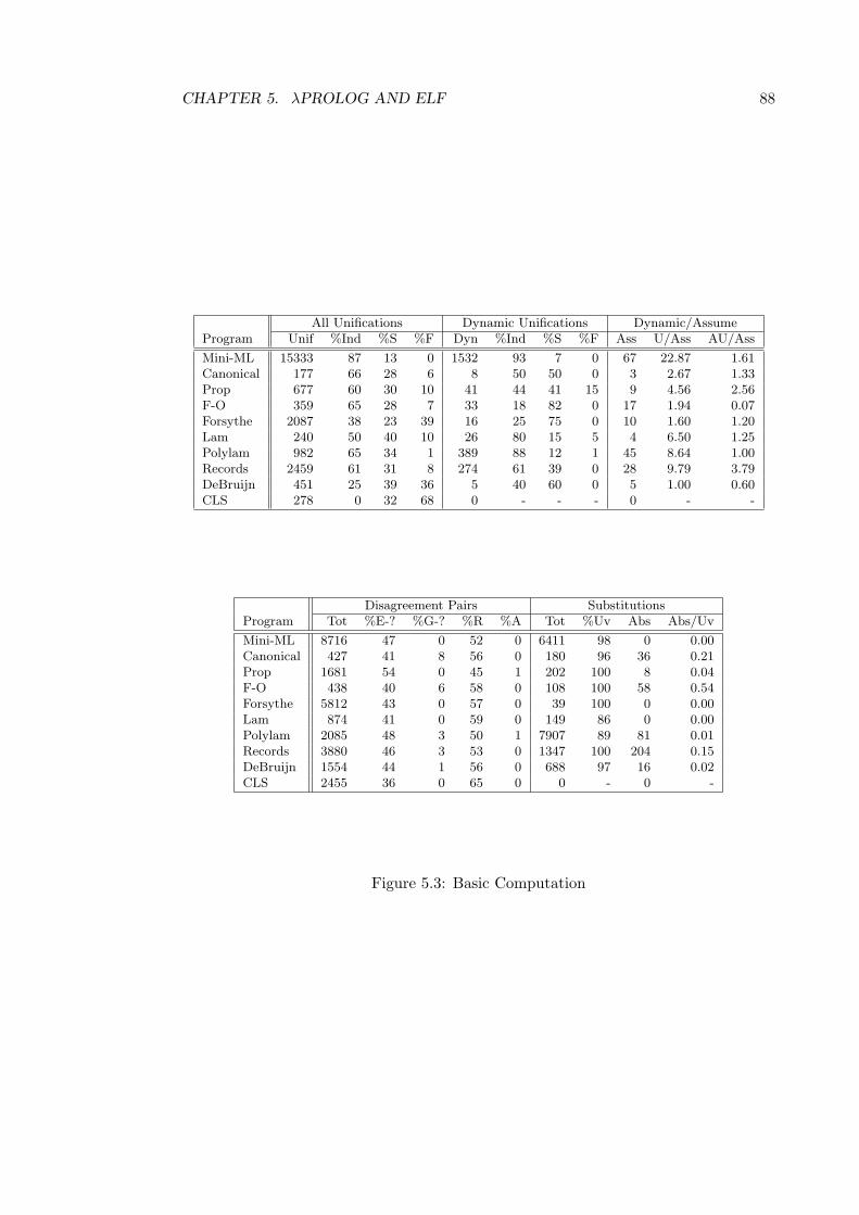
CHAPTER 5. λPROLOG AND ELF 88
All Unifications Dynamic Unifications Dynamic/AssumeProgram Unif %Ind %S %F Dyn %Ind %S %F Ass U/Ass AU/Ass
Mini-ML 15333 87 13 0 1532 93 7 0 67 22.87 1.61Canonical 177 66 28 6 8 50 50 0 3 2.67 1.33Prop 677 60 30 10 41 44 41 15 9 4.56 2.56F-O 359 65 28 7 33 18 82 0 17 1.94 0.07Forsythe 2087 38 23 39 16 25 75 0 10 1.60 1.20Lam 240 50 40 10 26 80 15 5 4 6.50 1.25Polylam 982 65 34 1 389 88 12 1 45 8.64 1.00Records 2459 61 31 8 274 61 39 0 28 9.79 3.79DeBruijn 451 25 39 36 5 40 60 0 5 1.00 0.60CLS 278 0 32 68 0 - - - 0 - -
Disagreement Pairs SubstitutionsProgram Tot %E-? %G-? %R %A Tot %Uv Abs Abs/Uv
Mini-ML 8716 47 0 52 0 6411 98 0 0.00Canonical 427 41 8 56 0 180 96 36 0.21Prop 1681 54 0 45 1 202 100 8 0.04F-O 438 40 6 58 0 108 100 58 0.54Forsythe 5812 43 0 57 0 39 100 0 0.00Lam 874 41 0 59 0 149 86 0 0.00Polylam 2085 48 3 50 1 7907 89 81 0.01Records 3880 46 3 53 0 1347 100 204 0.15DeBruijn 1554 44 1 56 0 688 97 16 0.02CLS 2455 36 0 65 0 0 - 0 -
Figure 5.3: Basic Computation

CHAPTER 5. λPROLOG AND ELF 89
All Unifications Dynamic Unifications Dynamic/AssumeProgram Unif %Ind %S %F Dyn %Ind %S %F Ass U/Ass AU/Ass
Extraction 878 89 11 0 165 82 17 1 54 3.05 0.54Mini-ML 2415 73 11 16 107 87 13 0 10 10.70 1.40CPS 162 59 41 0 72 57 43 0 48 1.50 0.65Prop 4957 67 25 8 509 71 14 15 71 7.17 2.10F-O 1140 69 27 4 27 0 100 0 13 2.08 2.08Lam 369 50 44 6 36 75 22 3 12 3.00 0.75DeBruijn 627 20 44 36 77 51 30 19 24 3.21 1.58CLS 333 30 42 28 0 - - - 0 - -
Disagreement Pairs SubstitutionsProgram Tot %E-? %G-? %R %A Tot %Uv Abs Abs/Uv
Extraction 1580 22 9 66 6 9016 96 1124 0.01Mini-ML 5872 17 1 76 6 3644 96 55 0.02CPS 592 24 34 54 0 1509 100 1029 0.68Prop 13809 35 3 63 1 12040 99 443 0.04F-O 6800 21 1 74 5 12716 99 38 0.00Lam 3464 22 2 74 3 1825 94 83 0.05DeBruijn 13441 15 1 71 13 14632 99 150 0.01CLS 5227 23 0 77 0 2 - 0 -
Figure 5.4: Proof Manipulation

CHAPTER 5. λPROLOG AND ELF 90
All Unifications Dynamic Unifications Dynamic/AssumeProgram Unif %Ind %S %F Dyn %Ind %S %F Ass U/Ass AU/Ass
Comp 5562 90 10 0 1532 92 8 0 67 22.87 1.61ExpComp 7200 70 10 20 1798 80 8 12 87 10.67 4.30ExpIndComp 7200 88 10 2 1798 92 8 0 87 10.67 4.30Trans 2159 70 11 19 107 86 14 0 10 10.70 1.40ExpTrans 5255 29 10 59 633 15 13 72 67 9.45 8.06ExpIndTrans 5255 76 11 13 633 84 13 3 67 9.45 8.06
Disagreement Pairs SubstitutionsProgram Tot %E-? %G-? %R %A Tot %Uv Abs Abs/Uv
Comp 2424 43 0 57 0 445 97 0 -ExpComp 10765 24 4 56 17 22743 100 778 0.03ExpIndComp 4251 32 10 52 8 15801 100 778 0.05Trans 5709 17 1 76 7 3612 96 55 0.02ExpTrans 27342 20 4 61 16 280679 97 2522 0.01ExpIndTrans 13482 17 8 65 12 264399 98 2522 0.01
Program Computation Transformation
Implicit 1.30 2.48Explicit 8.48 155.09Explicit-Indexed 5.80 145.89
Figure 5.5: Mini-ML comparison

CHAPTER 5. λPROLOG AND ELF 91
• Mini-ML [117]
An implementation of Mini-ML, including type-checking, evaluation, and the typesoundness proof. Because of the large number of cases, indexing has a strongereffect than in all other examples.
• CPS — Interpretation of propositional logics and CPS conversions [60, 142]
Various forms of conversion of simply-typed terms to continuation-passing andexception-returning style. Substitutions are all parameter substitutions, and uni-fication involves an unusually large number of Gvar-anything cases. The redun-dant type computations are very significant in this example — all the queries arelevel 2 judgments.
• Canonical — Canonical forms in the simply-typed lambda-calculus [139]
Conversion of lambda-terms to canonical form. A small number of non-parametersubstitutions arise, but mostly unification is first-order. Here, too, there is muchredundant type computation.
• Prop — Propositional Theorem Proving and Transformation [66]
This is mostly first-order. In the transformations between various proof formats(natural deduction and Hilbert calculi), a fairly large number of assumptions arise,and are quite heavily used. Unification involves a large number of Evar-anythingcases.
• F-O — First-order logic theorem proving and transformation
This includes a logic programming style theorem prover and transformation ofexecution trace to natural deductions. There is rather little abstraction.
• Forsythe — Forsythe type checking
Forsythe is an Algol-like language with intersection types developed by Reynolds[145]. This example involves very few substitutions, all of which are parametersubstitutions. Thus the runtime behavior suggests an almost entirely first-orderprogram, which is not apparent from the code.
• Lam — Lambda calculus convertibility
Normalization and equivalence proofs of terms in a typed λ-calculus. A relativelyhigh percentage of the substitutions are non-parameter substitutions.
• Polylam — Type inference in the polymorphic lambda calculus [137]
Type inference for the polymorphic λ-calculus involves postponed constraints,but mostly parameter substitutions. Unification can be highly non-deterministic.This is not directly reflected in the given tables, as this is the only one of our

CHAPTER 5. λPROLOG AND ELF 92
examples where any hard constraints are delayed at run time (and in only 10instances). In fact, one of these hard constraints remains all the way to theend of the computation. This indicates that the input was not annotated withenough type information (within the polymorphic type discipline, not within theframework).
• Records — A lambda-calculus with records and polymorphism
Type checking for a lambda-calculus with records and polymorphism as describedin [67]. This involves only parameter substitutions, and assumptions are heavilyused.
• DeBruijn [63]
A compiler from untyped λ-terms to terms using deBruijn indices, including acall-by-value operational semantics for source and target language. The proofmanipulation queries check compiler correctness for concrete programs. Indexingworks quite poorly, and an unusually large number of Abst-Abst cases arise inunification.
• CLS [63]
A second compiler from terms in deBruijn representation to the CLS abstractmachine. Simple queries execute the CLS machine on given programs, proofmanipulation queries check compiler correctness for concrete programs. This isalmost completely first-order.
Overall, the figures suggest quite strongly that most unification is either simpleassignment or first-order (Herbrand) unification, around 95%, averaged over all exam-ples. Similarly, substitution is the substitution of parameters for λ-bound variables inabout 95% of the cases. The remaining 5% are substitution of constants, variables, orcompound terms for bound variables. These figures do not count the substitution thatmay occur when clauses are copied, or unifications or substitutions that arise duringtype reconstruction.
Finally, we compare the Mini-ML program with a version written using explicitsubstitution, to evaluate the effects of a syntactic restriction along the lines of Lλ. Thecomputation queries had to be cut down somewhat because of memory restrictions. InFigure 5.5 we show the same data as above for the computation and transformationqueries with and without explicit substitution. We also show a version with explicitsubstitution with the substitution code rewritten to take better advantage of indexing.Then we compare the CPU times (in seconds) for the two sets of queries for all threeversions of the program, using a slightly modified2 Elf version 0.2 in SML/NJ version0.80 on a DEC station 5000/200 with 64MB of memory and local paging. Theseresults show that there is a clear efficiency disadvantage to the Lλ restriction. Notethat the disadvantage is greater for the transformation queries, since a longer proofobject is obtained, resulting in a more complicated proof transformation. Explicit
2The modification involves building proof objects only when needed for correctness.

CHAPTER 5. λPROLOG AND ELF 93
substitution increases the size of the relevant code by 30%.3 Substitutions dominate thecomputation time, basically because one meta-level β-reduction has been replaced bymany substitutions. These substitutions should all be parameter (Uvar) substitutions,which suggests that some (but clearly not all) of the performance degradation couldbe recovered through efficient Uvar substitution. See the previous footnote on whynon-parameter substitutions still arise in the proof transformation examples. We willdraw heavily on these results in Chapter 11.
3Actually, the meta-theory was not completely reduced to Lλ, because type dependencies in theverification code would lead to a very complex verification predicate. We estimate that the code sizewould increase an additional 5% and the computation time by much more than that.

Part III
Implementation Techniques
94

Chapter 6
Implementation Strategy
The remainder of this thesis deals with efficient implementation of CLP systems. In thischapter, a general strategy is outlined for dealing with the efficiency issues introducedin Chapter 3, largely by taking advantage of the observations made in that chapter andillustrated in Chapters 4 and 5. The following chapters discuss the implementationtechniques in detail, illustrated by the implementation of a CLP(R) compiler. Finally,a strategy for applying these techniques to λProlog and Elf is outlined.
Consider the basic implementation model for a CLP language, as shown in Figure6.1. The inference engine, using a goal and the rule base, controls search through therule base. During the search, it passes constraints to the constraint solver, which arethen added to a collected set of constraints. If the newly augmented set is consistent,the answer yes is returned, and otherwise no is returned. Whenever the inferenceengine needs to backtrack through the search tree, it sends a backtrack signal to theconstraint solver for every time the most recent remaining constraint is to be removedfrom the current set of constraints. The set of constraints currently stored in theconstraint solver at any given time will often be referred to as the solved form. Finally,when it is time to output an answer constraint, the inference engine gives the constraintsolver the set of variables on which the solved form is to be projected, and the result isoutput. To avoid confusion, note that our use of the term “inference engine” is not quitestandard. In discussing Prolog systems, it tends to be used to describe both the searchand unification components. Here we use it to refer only to the search (resolution)component.
Our discussion of implementation will focus on the following aspects:
• Suitable data structures for dealing with the incremental nature of constraintsolving in the context of backtracking.
• Organization of the constraint solver, and assignment of additional responsibilityto the inference engine, such that simple constraints are executed as efficiently aspossible.
• A conceptual framework for specifying delayed constraints, and resulting datastructures, so that constraints may be delayed and awakened efficiently.
95
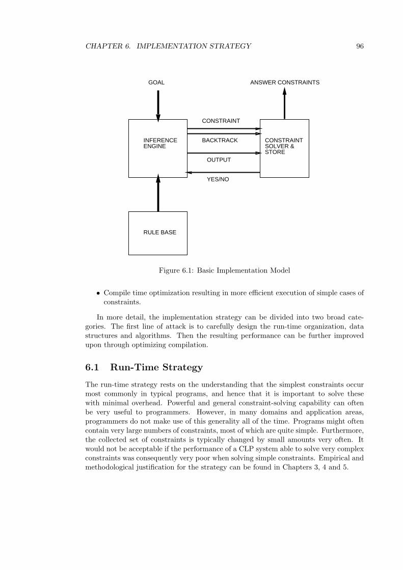
CHAPTER 6. IMPLEMENTATION STRATEGY 96
CONSTRAINT
BACKTRACK
YES/NO
OUTPUT
CONSTRAINT SOLVER &STORE
INFERENCE ENGINE
GOAL
RULE BASE
ANSWER CONSTRAINTS
Figure 6.1: Basic Implementation Model
• Compile time optimization resulting in more efficient execution of simple cases ofconstraints.
In more detail, the implementation strategy can be divided into two broad cate-gories. The first line of attack is to carefully design the run-time organization, datastructures and algorithms. Then the resulting performance can be further improvedupon through optimizing compilation.
6.1 Run-Time Strategy
The run-time strategy rests on the understanding that the simplest constraints occurmost commonly in typical programs, and hence that it is important to solve thesewith minimal overhead. Powerful and general constraint-solving capability can oftenbe very useful to programmers. However, in many domains and application areas,programmers do not make use of this generality all of the time. Programs might oftencontain very large numbers of constraints, most of which are quite simple. Furthermore,the collected set of constraints is typically changed by small amounts very often. Itwould not be acceptable if the performance of a CLP system able to solve very complexconstraints was consequently very poor when solving simple constraints. Empirical andmethodological justification for the strategy can be found in Chapters 3, 4 and 5.

CHAPTER 6. IMPLEMENTATION STRATEGY 97
The specifics of this strategy can be summarized as follows:
• Classify and prioritize constraints, reflecting:
– estimated relative frequency of occurrence;
– relative cost of solving.
• Treat constraint solving as generalized unification, thus making the Prolog casemost important.
• Avoid general constraint solving machinery where possible.
• Design data structures to favor simple cases.
• Check for hard constraints that should be awakened without undue impact onthe efficiency of constraint solving.
• To facilitate backtracking, store details of all changes to the collected constraintset, rather than backing up all or part of it at every change.
The organization and restriction of the constraint solver is addressed in Chapters 7and 8, while data structures for incrementality and efficient backtracking are discussedin Chapter 9. These ideas were incorporated in a CLP(R) interpreter project in whichthe author collaborated, and further refined in the compiler-based system discussedbelow. The system was based on structure-sharing Prolog interpreter technology, asexemplified by C-Prolog. The performance on most Prolog programs is comparablewith such Prolog interpreters, and performance for arithmetic constraints has beensufficiently good for non-trivial applications to be implemented.
6.2 Compile-Time Strategy
The usual approach to the compilation of Prolog rests on two basic ideas:
• The unification algorithm can usefully be partially evaluated with respect to thepartially constructed terms appearing in rules.
• The backtracking-based execution model for Prolog can be mapped onto thestack-based paradigm for executing conventional programming languages.
Most modern Prolog compilers are based on the Warren Abstract Machine (WAM),defined by D. H. D. Warren [189]. This is an abstract machine specification includingvarious stacks and registers, together with a special-purpose target instruction set forcompiling Prolog. The reader seeking a tutorial introduction to this style of Prologcompilation should consult the book by Aıt-Kaci [2]. The WAM has been used in theimplementation of a number of commercial systems, many emulating the WAM at runtime, others generating native code.

CHAPTER 6. IMPLEMENTATION STRATEGY 98
Since Prolog performance of CLP systems is a high priority, it is natural to wantto apply the usual Prolog compilation techniques to these languages. However, thequestion is whether compilation can be of benefit to solving constraints more generalthan Prolog unification. Chapter 10 gives a detailed description of an approach tocompiling CLP languages, with a particular emphasis on CLP(R), This rests partlyon the assumption that certain simple kinds of constraints can be detected easily atcompile time, so that with the use of peephole optimization these might be executedmore efficiently than if such an analysis were to be carried out at run time, as mentionedabove. For compiling CLP(R), the Constraint Logic Arithmetic Machine (CLAM) isdescribed in Chapter 10. This is an extension of the WAM with instructions and extrastructures for arithmetic constraints. These ideas have been incorporated in IBM’scompiler-based implementation of CLP(R), in which the author participated. This hasnow been widely available and in use for over two years, and has been the platformfor a number of large applications. Significantly, the performance of the CLAM-basedCLP(R) system on Prolog programs is close to that of the major commercial Prologimplementations. Furthermore, there is a significant performance improvement overthe interpreter mentioned above for arithmetic constraints.
It has long been observed that Prolog programs could be executed more efficientlyif they were specialized with respect to certain classes of allowed queries. Given a classof allowed queries specified in some formal language, it is possible to analyze a programglobally to determine various properties of its execution for queries that are in thisclass. These properties include determinism, types of variables, and modes (informa-tion about a variable having a certain level of instantiation at a certain point in anexecution). The best known technique for such global analysis is abstract interpreta-tion. This is based on the idea of executing a program on a special domain knownas the abstract domain, which captures the kinds of properties that are desired. Theprogram is executed with respect to a query that represents the set of allowed queriesfor the program, using arguments built up from the abstract domain. For an overviewof abstract interpretation, the reader should consult [40], although the literature on thistopic is quite large. In their respective dissertations, Van Roy [148] and Taylor [181]have shown that abstract interpretation has the potential to enable Prolog compilersto achieve performance comparable to that of compilers for conventional languages.
Abstract interpretation of CLP programs was described by Marriott and Søndergaard[114], and Jørgensen et al [91] describe various global analysis techniques for CLP(R),but otherwise little work has been done on global analysis for CLP languages. Theapproach to compiling CLP languages, described in detail in Chapter 10 rests on thethe following observations:
• Local optimizations can help to solve obviously simple constraints efficiently.
• Parts of programs (say modules) tend to be called in a number of specific ways,some of which result in apparently complex constraints collapsing into simple (orsimpler) cases.
• Such special cases can be detected by state-of-the-art program analysis techniques

CHAPTER 6. IMPLEMENTATION STRATEGY 99
(beyond the scope of this thesis) and efficient code can be generated by multiplespecialization of these modules.
• Abstract machines can be designed to take advantage of the above compilationideas.
While a compiler based on these techniques has not yet been implemented forCLP(R), the CLAM has been extended to take advantage of the sort of informationthat can be obtained from global analysis of CLP(R) programs. The CLAM emu-lator that forms the core of the compiler-based CLP(R) system described above hasbeen extended to obtain empirics on hand-compiled programs. This has demonstrateddramatic performance improvements for a number of programs with various allowedqueries. These results are also described in Chapter 10.
6.3 Summary
This major difference between this part of this thesis and other work that has been doneon CLP(R) implementation is the emphasis on handling frequently-occurring specialcases of constraint solving well. This difference in emphasis results from the fact thatthese implementation efforts have been driven by a study of programming methodology,and thus static and dynamic properties of programs, rather than a classical (operationsresearch-oriented) view of constraint solving.

Chapter 7
Organization of Solvers
The basic architecture for a CLP system as outlined in Figure 6.1 in Chapter 6 is inpractice not adequate for two reasons. First, it does not facilitate delay, which we haveargued to be essential. Second, it assumes that constraint solving is all handled by amonolithic “black box”, the details of which are invisible to the inference engine andother modules. For most CLP languages, such an abstraction cannot be adhered to inpractice if acceptable performance is to be attained. It needs to be broken down in twoways:
1. A typical constraint domain will consist of various subdomains, with possiblymore than one kind of constraint on each. Different individual solvers will beneeded to solve different kinds of constraints, to hide the complexity of solvingone kind from the algorithm implementing another.
2. Details of constraint solving will have to be made available to the inference engine,at least to facilitate rule indexing.
In this chapter we develop an implementation model to facilitate delay mechanismsand for multiple constraint solvers, which may interact more closely with the infer-ence engine. After generalizing the basic implementation model to one with delay, weexplore the required properties of multiple constraint solvers for efficiency and correct-ness. Finally, we use the organization of the constraint solver modules in the CLP(R)interpreter (and subsequent compiler-based implementation) to illustrate how theseprinciples are applied in practice.
7.1 Adding Delay to The Implementation Model
Figure 7.1 shows a generalization of the basic implementation model of Figure 6.1 toincorporate delay. This is still a generic model, in that it is not specialized for anyparticular domain. However, it illustrates some of the ideas that will be taken furtherbelow. First we have the notion of a constraint being too “hard” for the generalconstraint solver, and thus being stored in the delay pool. This is really an activeagent, constantly monitoring the constraint solver to check when a constraint becomes
100

CHAPTER 7. ORGANIZATION OF SOLVERS 101
CONSTRAINT
YES/NO
CONSTRAINT SOLVER &STORE
INFERENCE ENGINE
GOAL
RULE BASE
ANSWER CONSTRAINTS
DELAYED
HARD AWAKENEDBACKTRACK& OUTPUT
Figure 7.1: Generic Implementation Model with Delay
RUNABLEQUEUE
DELAY POOL
CHECKIF READY
NEW HARD CONSTRAINTS SOLVER STATE
BACK TO SOLVER:NO LONGER HARD
OUTPUT
Figure 7.2: Delay/Wakeup Mechanism

CHAPTER 7. ORGANIZATION OF SOLVERS 102
“runnable”, so that it can be awakened before the next inference. When a constraint isawakened it re-enters the solver as if it were a new constraint, except it is now knownnot to be hard (although its processing may give rise to further hard constraints). Therunnable constraints must be queued because one change to the solver state can resultin several constraints being awakened. The first of these can make another change to thesolver state awakening more constraints, and so on. Figure 7.2 describes this in somemore detail. Henceforth we dispense with representing flow of control (for modules suchas backtracking and output) in these diagrams, and just note that every componentof the constraint handling mechanism conceptually must be able to handle these. Thedetailed implementation of the delay/wakeup mechanism can actually be quite complex.The conceptual framework and implementation strategy will be described in detail inChapter 8.
7.2 Multiple Constraint Solvers
The most straightforward use of multiple constraint solvers is to deal with compositedomains: those composed from a number of simple domains. For example, the domainof CLP(R) is composed of uninterpreted functors and real arithmetic. In such cases itis desirable to combine multiple solvers because algorithms are typically available forthe simple domains. Then the collected set of constraints is deemed inconsistent if andonly if one of the solvers finds that it has an inconsistent store, but the whole point isthat each solver should see only the constraints on that domain. For obvious efficiencyreasons it is necessary to limit the number of constraints in each store. Most comedirectly from the input constraints, but others can be generated by the other solvers,to link all the constraints together correctly. Thus we need a formal understanding ofthe minimal amount of information that must be shared.
Typically, the simple domains do not share function symbols. This case has beenstudied quite heavily. In [130], it is shown that it is sufficient for each solver to exportonly the equations between pairs of variables to the other solvers, and disjunctions ofsuch equations that are implied by its store. For solvers that cannot imply disjunctionsof such equalities (so-called convex domains), only individual equations are transferred.The result is interesting both in theory and practice. Other, more specific, work onsuch combinations of solvers includes that by Kaplan [92] on the theory of arrayswith constant indices, by Shostak [160] on Presburger arithmetic with uninterpretedfunction symbols, and by Suzuki and Jefferson [178] on Presburger arithmetic arraysand uninterpreted function symbols.
Unfortunately, the property required for this result is too restrictive for an importantuse of multiple solvers. Sometimes a single domain can include constraints of differingdifficulty, so a low-overhead solver is desirable for the easier constraints, and a morecomplex, higher-overhead solver is used for the rest. As will be discussed below, thisis the case for CLP(R). It is a very valuable technique for implementing CLP systemsefficiently, but the above correctness result does not hold, as often function symbolsare shared. Furthermore, no corresponding result is available, so that ensuring the
CHAPTER 7. ORGANIZATION OF SOLVERS 103
correctness of multiple solvers combined in this way must be done on a case by casebasis.
For this reason, we formalize the exact correctness criterion. Consider a CLP systemwith a solver component consisting of n solvers S1 to Sn, with respective constraintstores C1 to Cn. The function φ maps a constraint to a solver index: an integer from1 to n. The function ψ selects all the relevant constraints from the stores of the othersolvers. In general this function will have to be conservative, but if we are to obtainthe benefits of multiple solvers, it should not be too conservative.
When a new constraint arrives, say, c, then we require that
|= ∃(C ∧ c) iff i = φ(c) ∧ Si |= ∃(Ci ∧ ψ(i, C1, · · · , Cn) ∧ c).
We will have nothing more to say about this correctness issue, and will not provethe correctness of the organization of solvers in CLP(R). However, it is worth lookingat an example to get an intuitive feeling for what can go wrong. As was shown inChapter 3, Prolog III tuple concatenation constraints (really word equations), give riseto integer constraints. Let us consider the execution of the query
?- U = X.Y, |U| = 3, |X| > 1, |Y| > 1.
The constraints in this query are unsatisfiable: if U is of length 3 and both X and Y areof length greater than 1, one of the latter must have non-integral length, which wouldnot make sense. Let us consider in some more detail how such a query would be solved.When the first constraint is selected, a number of additional integer constraints result:
1. |U| = |X| + |Y|
2. |U| >= 0
3. |X| >= 0
4. |Y| >= 0
Then the remaining constraints only interact with the integer solver, and in conjunctionwith the four integer constraints resulting from the original word equation, have nointeger solution. The interesting point is that Prolog III does not have an integersolver. Now it is not sufficient to mark the length of any word variable to be integral,since the rational arithmetic solver only determines that there is a rational solution. Inthe example above a rational solution exists — in fact there are infinitely many, andthis is the problem. Because non-integer solutions are actually not generated in thiscase, Prolog III fails to detect that the query above is unsatisfiable. In fact this is quiteconsistent with the stated behavior of Prolog III, since word equations are delayed untilthe first argument of a concatenation is of known length. Hence we have to go deeperto see what the problem is. Consider the query
?- U = X.Y, |X| = 2, |U| > 2, |U| < 3.

CHAPTER 7. ORGANIZATION OF SOLVERS 104
The query is again unsatisfiable, but the word equation is awakened by the integerconstraint |X| = 2, so a definitive answer would be expected. However, the integerequations generated do have a rational solution, so Prolog III again fails to detectthat the query is unsatisfiable. Finally, it is reasonable to ask what model of solvingword equations could be supported by just solving rational arithmetic constraints. Foran equation of the form X = Y + Z to have an integer solution whenever it has anarithmetic solution, any two of the variables must be ground. This means that onlylocal propagation can be supported in this way, in which case the arithmetic equationson lengths of word equations become quite useless.
In summary, while the benefits of using multiple communicating constraint solversare considerable in practice, the system designer must consider the correctness issuescarefully. Implementing a CLP system with such a constraint solving structure is anon-trivial engineering problem.
7.3 Interpreting CLP(R)
The organization of constraint solving in a CLP(R) interpreter provides a good oppor-tunity to study the runtime aspects of constraint solving. The material in this sectionis discussed from a somewhat different viewpoint in [88].
Here the generic implementation model is modified with the aims of:
1. solving Herbrand (unification) constraints with the efficiency of a Prolog inter-preter;
2. performing simple arithmetic test and local propagation efficiently;
3. solving linear equations without concern for unrelated linear inequalities.
To satisfy the first objective, it was clear that the inference engine would have to beintegrated with a Prolog-style unifier for Herbrand constraints. The engine is an adap-tation of a structure-sharing Prolog interpreter. There are two central data structures,both of which are stacks. The major step performed by the engine is the creation ofbindings of certain variables; this is activated either in the reduction step for a subgoal,or when certain kinds of equations are encountered. The following section elaborates onthis. As will be described below, when arithmetic constraints are encountered, they arepassed to the arithmetic constraint solver, which is really a cluster of three constraintsolvers, as follows:
• an interface, which evaluates complex arithmetic expressions and transforms con-straints to a small number of standard forms;
• an equation solver, which deals with linear arithmetic equations that are toocomplicated to be handled in the unifier and interface;
• an inequality solver, which deals with linear inequalities;

CHAPTER 7. ORGANIZATION OF SOLVERS 105
In this case, as has been mentioned before, nonlinear equations are considered hardconstraints, and are delayed.
The interface between the unifier and linear solvers transforms constraints into astandard form. In this transformation, the input constraint is broken up into partsthat are handled by different modules of the solver. The interface does some con-straint satisfaction on its own, thus further lessening the need to use the solver. Theequation solver maintains its equations in parametric solved form, that is, some vari-ables arising from program execution are described in terms of parametric variables.The equation solver may need to send some equations to the inequality solver. Theinequality solver may communicate back to the equation solver. This happens whenimplicit equalities, that is, equations entailed only by non-strict inequalities, have beencomputed. The nonlinear constraint handler obtains nonlinear equations to be delayedfrom the interface. Based on information in the linear equality solver, it sometimesawakens these constraints and ships them to that linear equation solver. The outputmodule then needs information from the engine/unifier, both linear solvers, and thenonlinear handler. The details of output are beyond the scope of this thesis: see [84]for an account of output in CLP(R). Figure 7.3 summarizes the activities allocated tothe various modules. In what follows, we describe the conceptual details behind theimplementation
7.3.1 Unification
Equations between non-arithmetic terms are handled by a standard unification algo-rithm to ensure that Prolog programs execute with Prolog speed. Furthermore, thisunification algorithm is closely associated with the inference engine so that terms canbe used for rule indexing. Many other kinds of equations, however, can also be handledusing the basic binding mechanism inherent in a unification algorithm. To define whatthese equations are, first define that a solver variable is one that appears in the collec-tion of constraints held by the arithmetic constraint solver. The kinds of constraintsthat are solved directly within the unifier are then described as follows:
• an equation between two non-solver variables;
• an equation between a non-solver variable and a solver variable;
• an equation involving an uninterpreted functor;
• an equation or inequality between two numbers, and
• an equation between a non-solver variable and a number.
The table in Figure 7.41 summarizes the binding mechanism used in the unificationalgorithm in the engine. As is usual, a variable can be either bound by pointing toanother term structure or to another variable forming a chain of references. We note,
1All variables mentioned there have been fully dereferenced. The empty slots represent the sym-metric cases.

CHAPTER 7. ORGANIZATION OF SOLVERS 106
SEARCH UNIFICATION
INTERFACE
INEQEQN BINDINGS
LINEAR INEQUALITIES
LINEAR EQUATIONS
NLIN AWAKENED
DELAYED
Inference Engine
Solver
Figure 7.3: CLP(R) Solver Organization

CHAPTER 7. ORGANIZATION OF SOLVERS 107
CLP(R) Unification TableT1
T2var s var number func arith func
var bind
s var T1→ T2 solvernumber T1→ T2 solver T1 = T2 ?func T1→ T2 n/a n/a T1 = T2 ?arith func interface interface interface n/a interface
Legend:
bind – Bind T1 to T2, or bind T2 to T1T1 → T2 – Bind T1 to T2var – ordinary free variables var – solver variablefunc – an uninterpreted functorarith func – an arithmetic functorT1 = T2? – are the topmost symbols equal?n/a – not applicable (corresponds to a type error)
Figure 7.4: Unification Table for CLP(R) Interpreter
however, that unlike in Prolog where a variable can only be free or bound to a term,variables in CLP(R) can belong to one of several distinct classes. In addition, a variablecan also be bound by means of an implicit binding, as explained below.
Some of the different cases covered in the unification table are:
• non-solver variable and non-solver variable;Choose one variable, and this choice may depend on the current run-time struc-ture, and then bind this variable to the other.
• non-solver variable and solver variable;To avoid invoking the constraint solver, the non-solver variable is bound to thesolver variable, rather than vice versa. This choice is crucial for efficiency.
• functor and any term;In case the term is a non-solver variable, a straightforward binding of this variableto the other term is performed. In case the term contains a functor, the principalfunctors of both terms are checked to see if they are equal. If so, then theircorresponding arguments are recursively unified.

CHAPTER 7. ORGANIZATION OF SOLVERS 108
• number and number;Because we use a floating-point implementation of numbers, we say that twonumbers are equal if they are sufficiently close to one another.
• non-solver variable and number;Since a non-solver variable does not appear in the solver, the variable can besimply bound to the number.
• solver variable and solver variable or number;The interface, and then perhaps the constraint solver, are invoked.
• arithmetic term and anything;Here also the interface, and then perhaps the constraint solver, are invoked.
This should become clearer as a result of the examples later in this section. Now let usconsider the special class of bindings between a variable and a number. Such a bindingcan occur in
• the unifier, when a non-solver variable is equated with a number that appears inthe program;
• the interface, when a non-solver variable is equated to a directly evaluable arith-metic expression;
• the equation solver, when a system of equations is solved and it follows thatcertain variables must take specific values;
• the inequality solver, as a consequence of an implicit equality, that is, an equationentailed by a number of non-strict inequalities.
The bindings in the first two cases are of an explicit nature, and have their counterpartsin standard logic programming systems. In the remaining two cases, the bindings occurin an implicit manner. For fast access to all these values, they are collected togetherin a central data structure, an implicit binding array, and this structure is accessiblefrom all modules in the system. Thus the implicit binding mechanism plays the role ofa cache.
Now that we have described the mechanism, let us consider its significance. Theempirical results in Section 5.6 show that a very large fraction of disagreement pairs arebetween a non-solver variable and an arithmetic variable (%VP). These are essentiallyarithmetic equations, but the binding mechanism we have described does not treatthem that way, and thus drastically reduces the number of constraints added to theequality solver. Furthermore, especially in the larger programs, the number of syntacticdisagreement pairs tends to dwarf the number of arithmetic constraints, showing theimportance of handling syntactic unification with minimal overhead.
Finally, we need to consider why this approach of doing as much constraint solvingas possible by unification cannot reasonably be taken further for CLP(R). To deal

CHAPTER 7. ORGANIZATION OF SOLVERS 109
with an equation of the form x = t, where t is an arithmetic term and x is a non-solvervariable, it would be quickest simply to bind the variable x to some representation oft. Such equations are, of course, always consistent with the constraints already storedin the solver, and hence the solver need not be invoked. It would become necessaryto dereference such variables x in any term encountered later. The solver would thenbe invoked only when the equation at hand, after having been dereferenced, does notcontain a non-solver variable as one operand. This implementation scheme, however,has two main drawbacks:
• Cyclic bindings;To implement dereferencing, the problem of cyclic references must be dealt with.This problem is analogous to the “occurs check” problem when dealing withnon-arithmetic terms. An important difference, however, is that an arithmeticequation whose representation contains a cyclic binding is not necessarily unsat-isfiable. Further, it is not possible to argue, as is done for most Prologs, thatcyclic bindings are pathological events and so the problem can be ignored.
• Thrashing behavior when backtracking;The use of arithmetic bindings can lead to long binding chains, which in turncan cause a thrashing-like behavior when backtracking takes place. For example,consider the program
loop(0).loop(I) :-
I > 0,p,loop(I - 1).
?- loop(N).
whose intent is to perform some operation p a total of N times, where N is givenas a number. Let I1, I2, etc, denote the various occurrences of the variable Icreated during execution. In the first iteration, I1 will be bound to the numberN ; then I2 will be bound to the term I1−1, I3 to (I1−1)−1, and in general, Ij willbe bound to a term of height j − 1. Now consider the unit rule and the recursivecall above, and note that in the jth iteration, an equation will be generated tocompare the term Ij − 1 with 0. The cost of evaluating this equation, becauseof the bindings associated with Ij , is proportional to j. Thus the overall cost ofexecuting the program, ignoring the cost of executing p, is proportional to N2 inthe best case. In contrast, if these equations are handled by a constraint solver,the cost can be linear in N .
Arithmetic bindings are not employed in the CLP(R) system because of these twoproblems.

CHAPTER 7. ORGANIZATION OF SOLVERS 110
7.3.2 The Interface
This module is called from the engine whenever a constraint contains an arithmeticterm. The interface first simplifies the input constraint by evaluating the arithmeticexpressions. If, as a result of this, the constraint is completely ground, then the ap-propriate test is made. If exactly one non-solver variable appears in the constraint andif the constraint is an equation, then an implicit binding is made, providing that it iseasy to solve for this variable. In all other cases, the solver is invoked.
Before the interface invokes the solver, it first transforms the simplified constraintinto a set of smaller constraints in canonical form. A constraint in canonical form isone of:
• an equation of the formn∑
i=1
ciXi = d
• an inequality of the formn∑
i=1
ciXi > d
• an inequality of the formn∑
i=1
ciXi ≥ d
• an equation of the form V ariable = c ∗ V ariable ∗ V ariable
where c, ci and d are real numbers, and all Xi are variables.
7.3.3 Linear Equations and Inequalities
The equality module is invoked in one of three ways.
1. From the interface with a linear equation in a form described above.
2. From the inequality solver with an implicit equality,
3. From the nonlinear constraint handler with an equation that has been awakened.
The equality solver returns true if the satisfiable constraints already stored in the solveras a whole are consistent with the input equation, and false otherwise.
The central data structure in the equality solver is a tableau that stores, in eachrow, a representation of some variable in the form of a linear combination of parametricvariables. The basic method of solution is a form of Gaussian elimination. A criticaloperation is that of simplifying substitutions, that is, the replacement of a chosenparametric variable by an equivalent parametric expression. Another critical operationis the communication between the equality and inequality solvers.

CHAPTER 7. ORGANIZATION OF SOLVERS 111
The Equation Tableau
The set of solver variables sent from the interface is partitioned by the equality solverinto two sets of variables: parametric and non-parametric variables. Linear equationsare stored in parametric solved form: using a matrix notation for convenience, this is apossibly empty collection of equations of which the ith one is of the form:
Xi = bi + ci,1 ∗ Ti,1 + ci,2 ∗ Ti,2 + · · ·+ ci,n ∗ Ti,n
where n ≥ 0, Xi is a non-parametric variable, the ci,j , 1 ≤ j ≤ n, are real numbercoefficients, and the Ti,j , 1 ≤ j ≤ n, are parametric variables. The variable Xi is calledthe subject of the equation.
Adding a New Linear Equation
Call the initial (empty) parametric solved form θ0. We now describe, given a parametricsolved form θj−1 and an input linear equation Ej , j ≥ 1, how to determine whetherθj−1 ∧ Ej is solvable. If so, we obtain a new solved form θj .
Let Cj be the result of substituting2 out each non-parametric variable X in Ej ,where X appears in the tableau θj−1, with the corresponding parametric form for X.
(1) If Cj is now of the form 0 = 0, then θj = θj−1, that is, the input constraint isalready implied by θj−1.
(2) If Cj is of the form 0 = c where c is a non-zero real number, then the collectionE1 ∧ E2 ∧ . . . ∧ Ej is inconsistent, and so θj does not exist. We simply returnnegatively.
(3) If Cj contains new variables, not currently in the solver, say X1, X2, . . . , Xm,m ≥ 1, then choose one of them, say X1, and rewrite Cj with X1 as the subject.X1 becomes a non-parametric variable and the remaining variables X2, . . . , Xm
become new parametric variables. The resulting equation is then added to θj−1
to obtain θj .
(4) If Cj contains no variables other than parametric variables, then choose one, sayT , and rewrite Cj with T as the subject. For efficiency reasons, the choice of sucha T is not arbitrary:
• we choose T , if possible, such that it does not appear in the tableau of theinequality solver;
• if, however, all the variables in Cj appear in the inequality solver, then wechoose, if possible, T such that T is a basic variable (the precise definitionof basic is not needed here) in the inequality solver;
• if, however, all the variables in Cj appear in the inequality solver as nonbasicvariables, then we may arbitrarily choose one of them to be T .
2Substitutions involve both replacement of terms for variables and collection of like terms.

CHAPTER 7. ORGANIZATION OF SOLVERS 112
Now the resulting equation, call it C′j , defines a substitution that enables parame-
ter elimination. That is, θj is obtained from θj−1 by substituting out the variableT using this substitution, and then adding the equation C
′j to the tableau. Note
that the variable T , once eliminated in this way, will never become a parametricvariable again except possibly as a result of backtracking. We will see later thatthe equation C
′j may need to be exported to the inequality solver. If so, the truth
value returned by the equality solver is the answer subsequently received fromthe inequality solver.
In summary, the equality solver returns affirmatively in case (1) and negatively in (2).In case (3), if m = 1, we must consider the possibility of nonlinear constraints beingawakened as a result of the input equation. Otherwise, we simply return affirmatively.Finally, in case (4), we must address the question of whether the inequality solver needbe invoked.
Awakening Delayed Constraints
When variables become ground (and this can happen in steps (3) and (4) above), it willbe necessary to communicate this fact to the nonlinear constraint handler. However, itis important that the nonlinear module be invoked only after the current equation hasbeen completely dealt with. This is because the nonlinear module can itself invoke theequality solver. Some complications arise in the implementation because of these twofacts:
• the equality solver uses one set of global data structures, and
• the equality solver and nonlinear handler are recursively dependent on each other.
We observe here that a negative response from the equality solver may be caused by anonlinear constraint that has been awakened.
Calling the Inequality Solver
The inequality solver is called by the equality solver if:
• we fall into case (4) above, and
• every variable in the equation C′j appears in the tableau of the inequality solver;
in which case the equation input to the inequality solver is C′j . The value returned by
the equality solver is just that returned by the inequality solver.The formal proof that only the above-mentioned kind of equations need be sent
to the inequality solver is beyond the scope of this thesis. Intuitively, we may reasonas follows: specific solutions to a parametric solved form can be obtained by simplyinstantiating the parametric variables with arbitrary values. In particular, we canuse values consistent with the constraints about parametric variables in the inequality

CHAPTER 7. ORGANIZATION OF SOLVERS 113
solver. Thus the only new additions to the equality solver that may be affected bythe inequality solver are those that make a parametric variable, which appears in theinequality solver, no longer independent from the other parametric variables. Thishappens only as described above. For a detailed description of linear inequality solvingin CLP(R), the interested reader should consult [174].
The empirical results in Section 4.5 show that not only are arithmetic inequalitiesless common than explicit arithmetic equations, but also that this treatment of inequal-ities often avoids the use of the Simplex solver. This is because the variables involvedare often ground by the time the inequalities are encountered, and they essentially justbehave like tests.
7.3.4 Some Examples of Constraint Flow
Let us begin by considering the query
?- X * X + Y * Y > 0, X + Y = 10, X - Y = 8.
The execution of this query proceeds as follows:
1. The first constraint is broken up into the three constraints
(a) T1 = X * X
(b) T2 = Y * Y
(c) T1 + T2 > 0
of which the first two are delayed, and the third is passed to the inequality solver.
2. The second constraint results in the parametric equation X = 10 - Y being passedto the equality solver, which stores it.
3. The third constraint is passed to the equality solver, which rewrites it using thepreviously stored parametric equation, and solves it giving Y = 1.
4. This value for Y is substituted throughout the equality solver, reducing the aboveparametric equation to X = 9.
5. The bindings for X and Y are propagated back to the unifier.
6. The same bindings are used to awaken the two delayed nonlinear equations, whichare put in the runnable queue as
(a) T1 = 1
(b) T2 = 81
7. T1 = 1 is taken from the head of the runnable queue, and passed to the equalitysolver, which considers T1 to be parametric since it was involved in an inequal-ity. Since all variables in the equation are then parametric, it is passed to theinequality solver, which essentially rewrites its one inequality to T2 > -1.

CHAPTER 7. ORGANIZATION OF SOLVERS 114
8. T2 = 81 is taken from the runnable queue, and similarly passed to the inequalitysolver, which simply confirms that 81 > -1 is true.
To further illustrate the role of the unifier, let us consider the query:
?- Y + 3 - Z = 0, f(X,Y) = f(U,U), X = 4.
Its execution proceeds as follows:
1. The first constraint results in, say, the parametric equation Y = Z - 3 beingstored in the equality solver, and both Y and Z being solver variables.
2. The second (Herbrand) equation is treated by the unifier, which in turn generatesthe equations
(a) X = UThis is treated by the unifier, say binding X to U.
(b) Y = UThis again is treated by the unifier. Since Y is a solver variable, U must bebound to Y.
3. In solving the third constraint, X deferences to Y, which is a solver variable. Hence,the equation Y = 4 must be passed to the equality solver, which uses its storedparametric equation to rewrite it, resulting in Z = 7, which is passed back to theunifier.
7.4 Summary
We have pointed out the importance of carefully organizing multiple constraint solversin a CLP system to improve efficiency. It is of central importance that simpler, morefrequently occurring classes of constraints be spared the overhead of general constraintsolving. Furthermore, different algorithms must be combined to solve constraints oncompound domains, and some aspects of constraint solving need to be available tothe inference mechanism for reasons such as the requirement for rule indexing. It hasalso been pointed out that there is a correctness issue involved in combining multiplesolvers, for which there seems to be no simple recipe. This is complicated by the factthat extra communication between solvers may be required for efficiency in additionto correctness. Finally, the organization of solvers in the implementations of CLP(R)demonstrate all of the three motivations for not treating a constraint solver as just asingle ”black box”.

Chapter 8
Managing Hard Constraints
A standard compromise approach to obtaining efficient constraint solvers has beento design a partial solver. That is, one that solves only a subclass of constraints,the directly solvable ones. These of course may or may not be consistent with thestate of the solver. The remaining constraints, the hard ones, are simply delayed fromconsideration when they are first encountered; a hard constraint is reconsidered onlywhen the constraint store contains sufficient information to reduce it into a directlysolvable form. It may then be processed, resulting in success or failure, or even morehard constraints. In the CLP(R) system, for example, nonlinear arithmetic constraintsare classified as hard constraints, and they are delayed until they become linear.
The key implementation issue is how to process efficiently just those delayed con-straints that are affected as a result of a new input constraint. Specifically, the cost ofprocessing a change to the current collection of delayed constraints should be relatedto the number and size of the delayed constraints affected by the change, and not to allthe delayed constraints. The following two items seem necessary to achieve this end.
First is a notion of how far a delayed constraint is from being awakened. Forexample, it is useful to distinguish the delayed CLP(R) constraint X = max(Y, Z),which awaits the grounding of Y and Z, from the constraint X = max(5, Z), whichawaits the grounding of Z. This is because, in general, a delayed constraint is awakenedby not one but a conjunction of several input constraints. When a subset of suchinput constraints has already been encountered, the runtime structure should relatethe delayed constraint to just the remaining kinds of constraints that will awaken it.
The other item is some data structure, call it the access structure, which allowsimmediate access to just the delayed constraints affected as the result of a new inputconstraint.
There are two main elements in this chapter. First is a framework for the specifica-tion of wakeup degrees which indicate how far a hard constraint is from being awakened.Such a formalism makes explicit the various steps a CLP system takes in reducing ahard constraint into a directly solvable one. The second element is a runtime structurethat involves a global pool of the delayed constraints, and an access structure for thatpool. A preliminary discussion of this work appears in [89].
115

CHAPTER 8. MANAGING HARD CONSTRAINTS 116
8.1 Delay Mechanisms
The idea of dataflow computation, see e.g. [9], is perhaps the simplest form of a delaymechanism since program operations can be seen as directional constraints with fixedinputs and outputs. In its pure form, a dataflow graph is a specification of the datadependencies required by such an operation before it can proceed. Extensions, such asthe I-structures of [10], are used to provide a delay mechanism for lazy functions andcomplex data structures such as arrays in the context of dataflow.
Carlsson [22] describes an implementation technique for freeze(X, G). While animplementation of freeze can be used to implement more sophisticated annotationslike wait and when, this will be at the expense of efficiency. This is mainly becausethe annotations can involve complicated conjunctive and disjunctive conditions. Sincefreeze takes just one variable as an argument, it is used in a complicated manner inorder to simulate the behavior of a more complex wakeup condition.
In general, the present implementation techniques used for Prolog systems havesome common features:
• The delay mechanism relies on a modification of the unification algorithm [22].This entails a minimal change to the underlying Prolog engine. In CLP systems,this approach is not directly applicable since there is, in general, no notion ofunification.
• Goals are awakened by variable bindings. Each binding is easily detectable (dur-ing unification). In CLP systems, however, detecting when a delayed constraintshould awaken is far more complicated in general. In this paper, this problem isaddressed using wakeup degrees, described in the next subsection.
• The number of delayed goals is not large in general. Thus, implementations inwhich the cost of awakening a goal is related to the number of delayed goals[22], rather than the number of awakened goals, can be acceptable. In a CLPsystem, the number of delayed constraints can be very large, and so such a cost isunacceptable. However, it should be noted that both the number of delayed goalsand the number of delayed constraints varies dramatically between programs.
8.2 Wakeup Systems
Presented here is a conceptual framework for the specification of operations for thedelaying and awakening of constraints. We begin by formalizing the notions of delayedand directly solvable constraints.
A hard constraint will be defined here as a primitive relation symbol, together witha mapping from its arguments to variables in the constraint solver. So, for example,the CLP(R) constraint
X + Y + Z * V = 3
would, internally, have to be broken up into the constraints

CHAPTER 8. MANAGING HARD CONSTRAINTS 117
X + Y + T1 = 3mult(T1, Z, V)
where all of the arguments of mult are variables.Formally, each hard/delayed constraint δ is a tuple 〈Ψ, θ〉 where Ψ is an n-ary hard
constraint symbol and θ is a substitution of variables potentially in Σ for the argumentvariables A1 to An of this instance of Ψ. Hence, in the example above, the secondconstraint is the informal representation of the formal hard constraint
〈mult, A1 ← T1, A2 ← Z,A3 ← V 〉.
The state of the constraint solver at any given time be denoted by a tuple 〈∆,Σ〉,where ∆ is the set of delayed constraints (meta-variable δ), and Σ is the set of directlysolvable (and hence solved) constraints (meta-variable σ), otherwise known as a solvedform.
To indicate how far a hard constraint is from being awakened, we associate witheach constraint symbol Ψ a wakeup system. Intuitively, a wakeup system correspondsto a finite state automaton, where the final state corresponds to a hard constrainthaving become directly solvable, and the other states, all of them initial, indicate howfar a delayed constraint is from being directly solvable. All of these states are knownas wakeup degrees. We will denote these using the possibly subscripted meta-variableD, and the degree corresponding to directly solvable constraints is distinguished withthe name awakened. Formally, for a given Ψ, the set
DSΨ = D0, · · · ,Dn, awakened
is a set of wakeup degrees for Ψ. For given Σ, each degree represents a subset of ∆such that all of DSΨ represents a partition of ∆. We will say δ 7→Σ D to mean thatdelayed constraint δ is mapped to degree D with respect to Σ. A delayed constraint inawakened is ready to be removed from ∆, and processed by the solver.
The point is that we want to execute the various finite state automata for eachof the delayed constraints, in order to manage their awakening (and, on backtracking,resuspension) efficiently. Taking the analogy further, we need to describe the transitionconditions. These are really the main point of the exercise, because they are intendedto be relatively inexpensive tests to determine when a constraint is coming closer tobeing awakened.
Associated with each wakeup degree D is a collection of pairs 〈W,N〉, where eachW is a generic wakeup condition and each N is a wakeup degree called the new degree.Each generic wakeup condition is a condition, expressed in some formal language, onthe argument variables of any delayed constraint assigned to the degree D. Such acondition is satisfied by a solved form Σ for a particular delayed constraint δ = 〈Ψ, θ〉if Σ |= Wθ. Here |= may be the entailment relationship used for constraint solving,or it may be a different one especially for awakening constraints. Note that Wθ willfrequently be referred to as a dynamic wakeup condition. In terms of the automatonanalogy, δ makes a transition from degree D to degree N under these circumstances.

CHAPTER 8. MANAGING HARD CONSTRAINTS 118
We will need to impose some structural conditions on wakeup systems so that theymake sense, but first we will give an example. To facilitate this and other examples inthis thesis, we need to develop a language as mention above, for describing the function7→Σ that partitions a ∆ for a particular Σ, and also the generic wakeup conditions.We emphasize that this choice of language is arbitrary, and the appropriate choice mayvary depending on the domain.
Let the meta-constants be a new class of symbols, and hereafter, these symbols aredenoted by α, β and γ. A meta-constant is used as a template for a (regular) constant.Define that a meta-constraint is just like a constraint except that meta-constants maybe written in place of constants. A meta-constraint is used as a template for a (regular)constraint.
To describe the partition function for a particular symbol Ψ, we simply assign toeach wakeup degree other than awakened a description of the hard constraints placedin that degree for a given Σ. Each such description is a pair (t, C) where
• t is a term of the form Ψ(t1, . . . , tn) where each ti is either a variable, constantor meta-constant,
• C is a conjunction of meta-constraints whose variables and meta-constants, ifany, appear in t. We allow the additional meta-constraint nonground(X) whichasserts that the variable X is not ground.
In our language, generic wakeup conditions have the same form as the meta-constraintcomponent of a degree description.
For the entailment relationship, let us use CLP(R) constraint satisfiability. Then7→Σ assigns a delayed constraint 〈Ψ, θ〉 to the degree D if the description of D is(Ψ(t1, . . . , tn), C), and ∃[Σ |=∗ (A1 = t1 ∧ · · · ∧ An = tn ∧ C)θ]. Here the existentialclosure is intended to deal with the meta-constants as if they were variables. Hence, anequation between a variable and a meta-constant is satisfied if the variable is groundwith respect to Σ, and then the meta-constant stands for this ground value.
Of course, we require that these descriptions form a partition of the possible in-stances of a Ψ constraint under any Σ. In CLP(R) for example, the wakeup system forthe hard constraint symbol pow, where pow(X,Y, Z) denotes X = Y Z , might includea degree assigned the description
pow(A,B, α), α 6= 0 ∧ nonground(A) ∧ nonground(B).
An instance of a pow constraint would be assigned to the corresponding degree if thefirst two arguments were not uniquely defined by Σ and the third was determined as anon-zero real number.
Consider once again the CLP(R) constraints involving pow. These constraints maybe partitioned into classes represented by the following wakeup degrees:
D0 : pow(A,B,C), nonground(A) ∧ nonground(B) ∧ nonground(C)D1 : pow(α,B,C), nonground(B) ∧ nonground(C)D2 : pow(A,α,C), nonground(A) ∧ nonground(C)D3 : pow(A,B, α), nonground(A) ∧ nonground(B)

CHAPTER 8. MANAGING HARD CONSTRAINTS 119
For the degree D0, an example wakeup condition is C = α. This indicates that whena constraint, e.g. Z = 4, is entailed by the constraint store, a delayed constraint suchas pow(X,Y, Z) is reduced to pow(X,Y, 4). This reduced constraint would be assignedthe new degree D3. Another example wakeup condition is A = 1, indicating that whena constraint such as X = 1 is entailed, a delayed constraint of the form pow(X,Y, Z)can be reduced to pow(1, Y, Z). This reduced constraint, which is in fact equivalentto the constraint Y = 1 ∨ (Y 6= 0 ∧ Z = 0), would be assigned the degree awakenedif the solver could deal with disjunction (which in CLP(R) it cannot). We note thatstipulating that a variable is nonground in this way is going to be rather cumbersome.Hence we will leave the stipulation out, and assume it to apply whenever nothing elseis said about a variable in a description. We exemplify some other uses of wakeupconditions below.
8.3 Structural Requirements of a Wakeup System
For the remainder of the discussion we need the concept of a path from one wakeupdegree to another, and that of such a path being satisfied by a solved form.
Definition 1 (Finite Path) A finite path from degree D to degree D′ is a sequenceof degrees Dj and connecting generic wakeup conditions WDj associated with them:
D1,WD1 ,D2, · · · ,Dn−1,WDn−1 ,Dn
for some n ≥ 1. If n = 1 then this is a null path. We write Σ ||=δ p for δ = 〈Ψ, θ〉 anda finite path p of length n if either
1. n = 1, or
2. for all j : 1 ≤ j < n, Σ |=WDjθ;
and for all 〈W,N〉 associated with Dn, Σ ∪ σ |=/ Wθ
Informally, we say that the path p is enabled by Σ for δ. We will need to disallow thepossibility of infinite paths being enabled, so we define them formally also.
Definition 2 (Infinite Path) A infinite path from degree D is a sequence of degreesDj and connecting generic wakeup conditions WDj associated with them:
D1,WD1 ,D2,WD2 , · · ·
We write Σ ||=δ p for δ = 〈Ψ, θ〉 and an infinite path p if for all j : 1 ≤ j, Σ |=WDjθ.
Now we are ready to state the structural conditions on wakeup systems. First, werequire that every transition of every delayed constraint toward being awakened can berepresented somewhere in the wakeup degree — essentially a soundness property.

CHAPTER 8. MANAGING HARD CONSTRAINTS 120
Definition 3 (Soundness) A wakeup system for Ψ is sound if for all ∆, Σ, δ =〈Ψ, θ〉 ∈ ∆, and σ whenever δ 7→Σ D and δ 7→Σ∪σ D′ we have that all of the followinghold:
1. There exists a path p from D to D′ such that Σ ∪ σ ||=δ p;
2. For all D′′ different from D such that there exists a path p′ from D to D′′ andΣ ∪ σ ||=δ p
′, we have D′ = D′′;3. There are no infinite paths q starting at D such that Σ ∪ σ ||=δ q.
The exact formulation of this condition needs some explanation. What we desire isthat the for any hard constraint δ and the addition of any constraint to Σ, the degreeassignment function 7→Σ and the wakeup system agree on how this addition affects thestatus of δ. This is captured directly in the first major condition. The complication isthat it is not possible to define any suitably small granularity of constraints added toΣ such that there will only be a single corresponding transition in the wakeup systemfor the individual hard constraint. This will usually be the case, but there will be caseswhere a single, very simple constraint added to the solved form triggers a chain or,as we have defined it above, a path of transitions. these paths will, in general, not beunique, since it is necessary to allow for the transitions occurring in any order, butof course they must all end up in the same degree. This is the reason for the rathercomplicated second major condition. As an example of where the complications arise,consider the sequence of constraints
pow(X,Y,Z), Y = Z, Z = 5
where the final constraint causes the pow constraint to be awakened straight from beingin the “least awakened” degree. Finally, as we will see in Chapter 11, it will sometimesbe necessary to allow cycles in wakeup systems (that is, non-null paths that begin andend at the same degree). However, the transition enabled by any solver state for eachdelayed constraint should be finite, so we must not allow the possibility of an infinitepath being enabled at the starting degree. Hence, we rule it out in the third majorcondition.
Our second structural requirement is that all of the wakeup degrees and dynamicwakeup conditions have some potential use, in a way that is locally sensible. We callthis minimality since we want to exclude useless additional components.
Definition 4 (Minimality) A wakeup system for Ψ is minimal if for all D and all〈W,N〉 associated with D there exist Σ, σ and δ = 〈Ψ, θ〉 such that all of the followinghold:
1. δ 7→Σ D2. δ 7→Σ∪σ N3. Σ ∪ σ |=Wθ

CHAPTER 8. MANAGING HARD CONSTRAINTS 121
W
D0
D1 D2 D3
ωωωωωω
ωωωωωω
ωωω
1
2 34 5
6 78
9
1011 12 13 14
15
Legend:
D0 : pow(A,B,C) D1 : pow(α,B,C), α 6= 0 ∧ α 6= 1D2 : pow(A,α,C), α 6= 0 ∧ α 6= 1 D3 : pow(A,B, α), α 6= 0 ∧ α 6= 1
ω1 : A = 0 ω2 : A = 1 ω3 : A = α ∧ α 6= 0 ∧ α 6= 1ω4 : B = 0 ω5 : B = 1 ω6 : B = α ∧ α 6= 0 ∧ α 6= 1ω7 : C = 0 ω8 : C = 1 ω9 : C = α ∧ α 6= 0 ∧ α 6= 1ω10 : B = α ω11 : C = α ω12 : A = αω13 : C = α ω14 : A = α ω15 : B = α
Figure 8.1: Wakeup degrees for pow/3
8.4 Example Wakeup Systems
The illustration in Figure 8.1 contains an example wakeup system for the CLP(R)constraint symbol pow. A wakeup degree is represented by a node, a wakeup condition isrepresented by an edge label, and the new degree of a reduced constraint is representedby the target node of the edge labeled with the wakeup condition that caused thereduction. Similarly, multiplication in CLP(R), denoted by the symbol mult, is shownin Figure 8.2.
Generic wakeup conditions can be used to specify the operation of many existingsystems which delay constraints. In Prolog-like systems whose constraints are overterms, awaiting the instantiation of a variable X to a ground term can be representedby the wakeup condition X = α. Awaiting the instantiation of X to a term of the formf(. . .), on the other hand, can be represented by ∃Y.X = f(Y ). We now give someexamples on arithmetic constraints. In Prolog-III, for example, the wakeup conditionX ≤ α could specify that the length of word must be bounded from above before furtherprocessing of the word equation at hand. For CHIP, where combinatorial problems arethe primary application, an example wakeup condition could be α ≤ X ∧ X ≤ β ∧β − α ≤ 4 which requires that X be bounded within a small range. For CLP(R),an example wakeup condition could be X = α ∗ Y + β, which requires that a linearrelationship hold between X and Y .
As another example, consider equational constraints involving two dimensional ar-rays. Let array(A,X, Y,E) denote the equation A[X,Y ] = E, which might sensiblybe delayed until all of A, X and Y are ground, at which time it becomes a simple

CHAPTER 8. MANAGING HARD CONSTRAINTS 122
D0
W
ω ωω2 3
1
Legend:
D0 : mult(A,B,C)
ω1 : A = αω2 : B = β ω3 : C = γ
Figure 8.2: Wakeup degrees for mult/3
equational constraint. Then a suitable wakeup system is shown in Figure 8.3.It might be expected that the wakeup system for word equations would be inter-
esting. However, assuming a sufficiently powerful decision algorithm for the arithmeticconstraints associated with word equations, we obtain only the very simple system inFigure 8.4, where concat(A,B,C) denotes the equation A.B = C. Initially, one mightexpect that there should be a separate degree for the situation where the length of Bis known, as this makes it easier to determine the length of A. However, if the decisionprocedure for the associated arithmetic constraints is sufficiently powerful, the lengthof A will always be supplied by that algorithm as soon as possible.
In CLP(Σ∗) [187], constraints of the form x ∈ e, where x is a string and e is aregular expression on strings, are delayed until they have a finite number of solutions.In general, this is the case when x is ground or e is ground and has no closure operators.To express this in our framework, we need to break these constraints into the three formsx ∈ y∗, x ∈ y.z and x ∈ y + z, where x, y, and z must be syntactically either variablesor strings. Denoting these constraint by clos, conc and or respectively, the wakeupsystem is shown in Figure 8.5.
8.5 The Runtime Structure
Here we present an implementational framework in the context of a given wakeupsystem. There are three major operations with hard constraints, which correspond tothe actions of delaying, awakening and backtracking:
1. adding a hard constraint to the collection of delayed constraints;
2. awakening delayed constraints as the result of supplying a directly solvable con-straint, and

CHAPTER 8. MANAGING HARD CONSTRAINTS 123
D0
D2
D5
W
D1 D3
D4 D6
ω ω ω
ω ωω ω ω ω
ω ω ω
31 2
4
56
7 89
10 11 12
Legend:
D0 : array(A,B,C,D)D1 : array(α,B,C,D) D2 : array(A, β,C,D)D3 : array(A,B, γ,D) D4 : array(α, β, C,D)D5 : array(α,B, γ,D) D6 : array(A, β, γ,D)
ω1 : A = α ω2 : B = β ω3 : C = γω4 : B = β ω5 : C = γ ω6 : A = αω7 : C = γ ω8 : A = α ω9 : B = βω10 : C = γ ω11 : B = β ω12 : A = α
Figure 8.3: Wakeup degrees for array/4
W
D0
ω0
Legend:
D0 : concat(A,B,C)
ω0 : |A| = α
Figure 8.4: Wakeup degrees for conc/3

CHAPTER 8. MANAGING HARD CONSTRAINTS 124
D0 D1
D2 D3
D4
D5 D6
W
ω ω
ω ω ω ω
ωω
ω ω ωω
ωω
1 2
9
4 5 7 8
10
1112 13
1415
16
ω ω3 6
WW
clos conc or
Legend:
D0 : clos(A,B)D1 : conc(A,B,C) D2 : conc(A, β,C) D3 : conc(A,B, γ)D4 : or(A,B,C) D5 : or(A, β,C) D6 : or(A,B, γ)
ω1 : A = α ω2 : B = εω3 : A = α ω4 : B = β ω5 : C = γω6 : A = α ω7 : C = β ω8 : A = γω9 : A = α ω10 : C = γω11 : A = α ω12 : B = βω13 : A = α ω14 : C = γω15 : A = α ω16 : C = β
Figure 8.5: Wakeup degrees for clos/2, conc/3 and or/3 in CLP(Σ∗)

CHAPTER 8. MANAGING HARD CONSTRAINTS 125
3. restoring the entire runtime structure to a previous state, that is, restoring thecollection of delayed constraints to some earlier collection, and restoring all aux-iliary structures accordingly.
We deal with the third operation, as well as other aspects of incrementality and back-tracking, in Chapter 9. The first of our two major structures is, for the time being,a pool of delayed constraints. Thus implementing the first operation, delaying a hardconstraint, simply requires adding a record to the pool, with the current form of theconstraint, and a field indicating its degree in the appropriate wakeup system.
Now consider the second operation. In order to implement this efficiently, it isnecessary to have some access structure mapping an entailed constraint γ to just thosedelayed constraints affected by γ. Since there are in general an infinite number ofentailed constraints, a finite classification of them is required. The classification we useis the set Ω∆,Σ of all dynamic wakeup conditions for all the delayed constraints in ∆ forthe current Σ, noting that delayed constraints may have dynamic wakeup conditionsin common. That is,
Ω∆,Σ = WDθ | δ = 〈Ψ, θ〉 ∈ ∆ ∧ δ 7→Σ D.
Of course this set will change every time ∆ or Σ change.We now specify an access structure that maps a dynamic wakeup condition into
a doubly linked list of nodes. Each node contains a pointer to a delay pool elementcontaining a delayed constraint1. Corresponding to each occurrence node is a reversepointer from the delay pool element to the occurrence node. For a generic wakeupcondition W we refer to the dynamic wakeup condition Wθ as DW. Call the listassociated with DW ∈ Ω∆,Σ a DW-list, and call each node in the list a DW-occurrencenode.
Initially the access structure is empty. The following specifies what is done for thebasic operations.
8.5.1 Delaying a new hard constraint
This operation adds new hard constraint δ = 〈Ψ, θ〉 to ∆, such that δ 7→Σ D. Firstadd a new delay pool element including its wakeup degree, D. Let W1
D, · · · , WnD be
the generic wakeup conditions of D. Then:
• Augment Ω∆,Σ with all of the DW1D, · · · , DWn
D.
• For each DW iD, insert into the DW i
D-list of the access structure a new occurrencenode pointing to the delay pool element for δ.
• Set up reverse pointers from the δ node to the new occurrence nodes.1The total number of occurrence nodes is generally larger than the number of delayed constraints.

CHAPTER 8. MANAGING HARD CONSTRAINTS 126
pow(X,Y,Z)
pow(Y,X,Y)D0
D0
A1 A2 A3 A4 A5 A6 A7 A8 A9
Delay Pool
C1
C2
Legend:
A1 : X = 0 A2 : X = 1 A3 : X = α ∧ α 6= 0 ∧ α 6= 1A4 : Y = 0 A5 : Y = 1 A6 : Y = α ∧ α 6= 0 ∧ α 6= 1A7 : Z = 0 A8 : Z = 1 A9 : Z = α ∧ α 6= 0 ∧ α 6= 1
Figure 8.6: The access structure
8.5.2 Responding to Changes in Σ
When Σ |= DW for some DW ∈ Ω∆,Σ, and this can happen whenever Σ is augmented,we need to update our structures.
Consider the DW-list L. Then consider in turn each delayed constraint pointed toby the occurrence nodes in L. For each such δ node, perform the following.
• Delete all occurrence nodes pointed to by the δ node., and delete DW from Ω∆,Σ.
• Update the node with the new wakeup degree of δ using the function 7→Σ. Thenperform the modifications to the access structure as described above when a newdelayed constraint is added.
Figure 8.6 illustrates the entire runtime structure after storing the two hard constraintspow(X,Y, Z) and pow(Y,X, Y ) in that order. Note that we are representing the hardconstraints informally. Figure 8.7 illustrates the structure after a new input constraintadds X = 5 to the solved form.
8.5.3 Optimizations
An important optimization is to merge DW-lists. Let there be lists corresponding tothe dynamic wakeup conditions DW1, . . . , DWn. These lists can be merged into onelist with the condition DW if
• adding any delayed constraint δ results in either (a) no change in any of the nlists, or (b) every list has a new occurrence node pointing to δ;

CHAPTER 8. MANAGING HARD CONSTRAINTS 127
pow(5,Y,Z)
pow(Y,5,Y)D2
D1
A4 A5 A6 A7 A8 A9
Delay Pool
C3
C4
Legend:A4 : Y = 0 A5 : Y = 1 A6 : Y = α ∧ α 6= 0 ∧ α 6= 1A7 : Z = 0 A8 : Z = 1 A9 : Z = α ∧ α 6= 0 ∧ α 6= 1
Figure 8.7: The new access structure
• for any Σ we have Σ |= DW iff Σ |= DW i for some 1 ≤ i ≤ n.
In the example of Figure 8.6, the three lists involving X can be merged into one listwhich is associated with the dynamic wakeup conditions X = α. Similarly for Y andZ.
This optimization is very frequently applicable, and of great importance. Recallthat the dynamic wakeup conditions must be monitored constantly, so it is essentialthat they be as simple as possible. It seems likely that delay with timely awakening willbe prohibitively expensive in systems where this optimization cannot be successfullyapplied.
8.5.4 Summary of the Access Structure
The access structure maps a finite number of dynamic wakeup constraints to lists ofdelayed constraints. The constraint solver is assumed to identify those conditions forwhich an entailed constraint is an instance. The cost of the basic operations can besummarized as follows.
1. Adding a new constraint δ simply involves determining its wakeup degree, creatinga delay pool entry, creating new occurrence nodes corresponding to δ and thesetting of pointers between the new delay pool entries and occurrence nodes. Thecost here is bounded by the number of generic wakeup conditions associated with(the degree of) δ.

CHAPTER 8. MANAGING HARD CONSTRAINTS 128
2. Changing the degree of a constraint δ involves replacing δ with δ′, determiningthe degree of δ′, and deleting and inserting a number of occurrence nodes. Sincethe occurrence nodes are doubly-linked, each such insertion and deletion can bedone in constant time. Therefore the total cost here is bounded by the numberof generic wakeup conditions associated with δ and δ′.
3. The cost of backtracking is important, and will be discussed together with thescheme for implementing it, in Chapter 9.
In short, the cost of one primitive operation on delayed constraints (delaying a newhard constraint, upgrading the degree of one delayed constraint, including awakeningthe constraint, and undoing the delay/upgrade of one hard constraint) is boundedby the (fixed) size of the underlying wakeup system. The total cost of an operation(delaying a new hard constraint, processing an entailed constraint, backtracking) ondelayed constraints is proportional to the size of the delayed constraints affected by theoperation.

Chapter 9
Incremental Constraint Solvers
A major challenge in implementing CLP systems stems from the required utility of theconstraint solvers. To be somewhat precise, a constraint solver maintains constraintswith respect to three kinds of operations for adding, removing and solving constraintsas follows:
• A state S = 〈S1, · · · ,Sn〉 where, for each i, Si = c1, · · · , cmi. The cj areconstraints, and Sn represents the set of constraints added since the most recentchoice point.
• A function cp that maps 〈S1, · · · ,Sn〉 to 〈S1, · · · ,Sn, 〉.• A function bt that maps 〈S1, · · · ,Sn〉 to 〈S1, · · · ,Sn−1〉.• A function solve that maps a state S = 〈S1, · · · ,Sn〉 and a constraint c to
– state 〈S1, · · · ,Sn ∪ c〉 and answer true if S1 ∪ · · · ∪ Sn ∪ c is satisfiable
– the old state S and answer false otherwise.
The original state is S = 〈〉. The function cp establishes a choice point – a state towhich the computation will backtrack on a subsequent failure. The function bt actuallyeffects such backtracking – rolling back to the state before the most recent choice point.The function solve, of course, tries to augment the solver state with a new constraint,checking that it is consistent with the constraints already there.
In this chapter we discuss the practical implications of this required utility, anda strategy for dealing with them. We discuss Prolog from this viewpoint, and thenconsider in detail the techniques for making the CLP(R) constraint solvers incremental.Much of this material is presented from a different viewpoint in [89] and [88].
9.1 Practical Implications of Incrementality
We should note that, in principle, any constraint solving algorithm can be used withoutmodification to provide this functionality. It can simply be re-invoked on the constraints
129

CHAPTER 9. INCREMENTAL CONSTRAINT SOLVERS 130
in S every time solve is invoked, and the states can be stored “outside” this solver.However, the following methodological and empirical observations about the expectednature of program execution show that such a naive approach, no matter how sophisti-cated the actual solving algorithm, is unlikely to be practical. These observations stemfrom Part II of this thesis.
In a given computation:
1. The number of constraints handled by solve can be extremely large (say tens ofthousands or more).
2. The number of constraints in the solver state S can also be extremely large,but typically, because of backtracking, it will not contain all of the constraintshandled.
3. The number n of sets Si of constraints between choice points can vary substan-tially, because some programs are much more deterministic than others.
4. For the same reason, the number of choice points can vary substantially.
5. While the set of constraints collected in the solver state may be very complicated,a large proportion of the individual constraints handled may be very simple.
Now, returning to the possibility of re-invoking a standard constraint algorithm forevery use of solve. Assuming (optimistically) that this algorithm takes time propor-tional to the number of constraints, the cost of using solve n times will be of order n2.This is unacceptable for a programming language.
The objectives of the design of a constraint solver are then to find an appropriatedecision algorithm and representation of state such that:
1. Individual invocations of solve should be affected more by the size and complexityof the constraint added, rather than of the constraints already stored in the state.We will call this the incrementality criterion.
2. The overhead of such invocations should not be excessive.
3. The space needed is not substantially more than linear in the size and number ofconstraints stored, with low overhead.
4. The cp function is implemented with very low overhead (virtually none) in spaceand time.
5. The cost of the bt function is dependent more on the amount the store was changedin adding the constraints now being be removed than on the size of the entirestore. This is just another facet of the incrementality criterion.
The phrase solved form is typically used to describe such a representation of theconstraint store. In general, the incrementality criterion is a rather vague notion. In itsstrictest form, it is virtually unattainable. Clearly, since the consistency of constraints

CHAPTER 9. INCREMENTAL CONSTRAINT SOLVERS 131
with the store is being tested, the cost will be somewhat affected by the number andcomplexity of the related constraints. That is, if all the variables in a new constraint arenew to the store, the size of the store should be irrelevant. On the other hand, if manyconstraints on the same variables are already being stored, that is an unreasonablerequirement. The notion of incrementality for some algorithms and representationsmay be made precise, but in general it will be an empirical property.
9.2 Incrementality and Prolog
Before moving on to CLP in general, let us consider to what extent unification in Prologis incremental. It it assumed that the reader is somewhat familiar with the standardProlog implementation techniques, especially the WAM.
We begin with the solve operation. Variable bindings in a Prolog interpreter es-sentially constitute an efficient solved form. When a new equation is encountered, thebindings of only some of the variables will have to be looked up, and likewise for thevariables in the terms they are bound to, and so on. However, if free variables areconsidered not to be in the solved form, the solved form is unchanged when a newequation is dealt with: it is only augmented. For example, consider the equation
f(X, g(V)) = f(h(Y, Z), U)
in the context of a solved form including the bindings
U = g(W)W = g(g(g(Y)))Y = g(g(Z))
but without any bindings for variables X or V. Since X is new, it is simply bound toh(Y, Z) and the bindings of Y and Z do not have to be considered at all — becausethe occurs check is omitted. The binding of U must be looked up to ensure that theprincipal functor can be a g, as it already is. Since V is new, it can simply be boundto W, whose binding again need not be considered. In summary, the cost of such aunification is only related to the size of the solved form in so far as parts of the solvedform are truly relevant to the unification. Nevertheless, unification is exponential inthe worst case.
Now we consider the operations involving backtracking. Recall that choice pointrecords are inserted into the runtime stack at nondeterministic branches, and somebindings are trailed1 so they can be undone on backtracking. However, backtracking isreasonably cheap, since:
• Bindings between activation records point from the newer variable to the older.This is useful if the binding is made before the first choice point after the cre-ation of the new activation record. The binding doesn’t need to be trailed, since
1The trail is a stack containing choice point records interleaved by a sequence of pointers to changedvariable locations that must be restored on backtracking.

CHAPTER 9. INCREMENTAL CONSTRAINT SOLVERS 132
the entire activation record will be removed on backtracking, thus removing thebindings.
• Bindings that are created pointing from above the most recent choice point recordare never trailed, for the same reason.
• The cp operation involves only creating a choice point record, and affects the costof subsequent bindings somewhat.
• The bt operation is relatively fast, since the trail simply lists locations wherebindings have to be deleted. This is because the solved form is never changedbeyond being further instantiated.
As we will see below, many of these fortunate properties are lost when other kindsof constraints have to be solved. Nevertheless, it is important to understand the impactof these properties on the performance of Prolog systems.
9.3 Strategy for Incremental Solvers
In general, to satisfy the above criteria, constraint solvers must typically rely on asolved form, with the implementation having the following properties:
1. When a new constraint is handled by solve, the relevant parts of the solved formmust be found quickly. That is, the solved form is essentially indexed on variables.Then the index is used to look up the parts relevant to the variables in the newconstraint. Ideally the index is an extension of Prolog variable bindings.
2. The satisfiability check usually involves attempting to construct a new solvedform, augmented with the new constraint. This should affect as little of thesolved form and supporting structures as possible. However, in the worst case, theentire solved form may have to be examined, and may also have to be extensivelymodified.
3. Since the solved form is, in general, modified rather than just further instantiated,simple trailing is insufficient. A tagged value trail is needed. On backtracking,the tag is used to determine what the inverse operation is, the usual address isused to determine where it is to be performed, and the value field, which mayinvolve a complex data structure, is used to perform the inverse operation.
4. In general, parts of the solved form will be changed many times between choicepoints. Hence, it is often best not to store all of the changes made for the purposesof backtracking. It may be better to backup an appropriate chunk of the solvedform when making the first change after a choice point. Then, subsequent changeswill not require trailing until another choice point is encountered. This works wellwhen appropriately small chunks can be identified, so they are not too expensiveto save.

CHAPTER 9. INCREMENTAL CONSTRAINT SOLVERS 133
5. Certain cross-referencing structures are too large and complex, and are changedtoo often to be worth trailing. It is better to rebuild these on backtracking. Thishas the advantage that no cost is incurred unless unless backtracking actuallytakes place.
For an interesting discussion of incrementality in constraint solving, see [55]. Thereis an important problem that we have not discussed so far: to date little work ondecision algorithms has taken incrementality into account. This means that for somedomains with a well known, efficient decision algorithm, at may be the case that either:
• there is no known incremental algorithm,
• the incremental algorithms are extremely slow, or
• there is a good incremental algorithm, but it is completely different to the bestdecision algorithm overall.
This factor limits the kinds of CLP languages that can be made practical, and henceneeds to be considered by the language designer.
9.4 Incrementality in Four Modules of CLP(R)
We now return to our major case study, and discuss the aspects of the implementationsof the various solver modules in the two CLP(R) implementations that are related toincrementality.
9.4.1 Unification
Unification in CLP(R) is sufficiently close to Prolog unification that it inherits theincrementality discussed above. However, even here the trailing (for backtracking)becomes somewhat more involved, since it is no longer the case that bindings mustsimply be undone. In particular, variables with implicit bindings (see Subsection 7.3.1)may have to go back to being of type s var.
9.4.2 Linear Equations
The algorithm for solving linear equations in CLP(R) was presented in Subsection7.3.3. The parametric solved form is represented mainly by a tableau of linked-lists.We also need a cross-reference table mapping each parametric variable to the list ofits occurrences within the main tableau. Additional structures include a tagged trailstack for backing up parametric forms that are about to be changed for the first timesince the last choice point. We now briefly outline the critical operations in the equalitysolver given this method of representation.

CHAPTER 9. INCREMENTAL CONSTRAINT SOLVERS 134
Parametric Substitutions
Given that a parametric variable T is to be replaced in the tableau, the first operationis to obtain, from the list in the cross-reference table corresponding to T , the list ofoccurrences of T in the tableau. The actual substitutions will have a cost proportionalto the length of this list.
An important consideration is how much this substitution enlarges the tableau.A straightforward heuristic for minimizing this number is to choose T such that itsfrequency in the tableau is minimal. At the present stage of our implementation,we have not found this to be necessary, and this suggests the frequencies tend to beuniformly distributed over the variables T we choose.
Backtracking
In CLP(R), as foreshadowed above, substitutions actually change the form of a para-metric equation. Thus when each row is changed for the first time after a choice point,the previous form, or some representation of it, must be stored. Given the data struc-tures above, it is clear that not only do the parametric forms themselves have to besaved for backtracking, but also the support structures, such as the cross-reference table,must be saved. Thus some complicated administrative mechanisms are also required,two of which need to be discussed.
First consider the parametric forms themselves. If we assume that the parametricform of a variable is, in general, going to be short, then it is reasonable to copy the entireequation when it is changed after a choice point. The extra space used is not a problemsince the number of parameters is small, and this method is very simple and hencefast. The alternative is to trail each change in an equation. While this “fine-grained”method usually benefits space utilization, it can suffer both from added complexity andreduced efficiency because many changes can go by between one choice point and thenext. Next consider the cross-reference table. As with parametric forms, we could saveentire entries corresponding to variables that are just about to be changed in some way.Instead, we choose to reconstruct the appropriate entries whenever parametric formsare restored upon backtracking. Since equations are typically small, reconstructingthe cross-reference table from the restored equation and the current equation is cheapand furthermore, this method does not incur any overhead when backtracking does notoccur.
Example
Figure 9.1 shows the major solver structures after the constraints X = Y + Z and W = 2* Z + 1 have been solved, with variables Y and Z chosen as parametric, and the othersas non-parametric. Figure 9.1 shows the state after a choice point has been encounteredand the additional constraint W = 5 has been solved. Notice how the old parametricforms have been saved but their index structure has not. In the trail fragments shown,P denotes that the variable was newly bound to a parametric form, and C denotes thata parametric form was changed. In the stack fragments, S denotes that the variable is

CHAPTER 9. INCREMENTAL CONSTRAINT SOLVERS 135
TRAIL STACK
P
P
P
P W
X
Y
Z S
S
S
S
0
1
1Y 1Z
2Z
Figure 9.1: Solver state after two equations
TRAIL STACK
P
P
P
P W
X
Y
Z S
S
S
S
0
1
1Y 1Z
2Z
5
1
1 1Y
C
C
C
C
Figure 9.2: Solver state after choice point and third equation

CHAPTER 9. INCREMENTAL CONSTRAINT SOLVERS 136
a solver variable, bound to a parametric form. We omit the details of distinguishingbetween parametric and non-parametric variables, and of implicit bindings.
9.4.3 Linear Inequalities
The details of the linear inequality solver are beyond the scope of this thesis — see [86]and [174]. It is based on an incremental formulation of the first phase of the two-phasesimplex method. The constraints that are actually sent to this solver are describedin Chapter 7. In the worst case, of course, the algorithm can be exponential in thesize and number of these constraints. However, each new constraint tends to take, onaverage, less than one pivot to be incorporated. The internal data structures of thissolver are very similar to those of the equality solver.
9.4.4 The Delay Pool
The main issue is maintaining the delay pool and access structure in the presenceof backtracking. For example, if changes to the structure were trailed using someadaptation of Prolog techniques, then a cost proportional to the number of entriescan be incurred even though no delayed constraints are affected. We return to theexponentiation example in Chapter 8 as our running example.
The delay pool itself is implemented using a stack. Thus delaying a hard constraintsimply requires a push on this stack. Additionally, the stack contains hard constraintsthat are reduced forms of constraints deeper in the stack. For example, if the hardconstraint pow(X,Y, Z) were in the stack, and if the input constraint Y = 3 wereencountered, then the new hard constraint pow(X, 3, Z) would be pushed, togetherwith a pointer from the latter constraint to the former. In general, the collection ofdelayed constraints contained in the system is described by the sub-collection of stackedconstraints that have no inbound pointers.
When a new hard constraint is being delayed, entering the appropriate record intothe delay pool consists of just pushing it onto the delay stack. When a new constraintis entailed, and some delayed constraint is affected, placing the form C′ of C in the delaypool changes somewhat. C′ is pushed onto the stack, setting up a pointer from C′ to C.
Figure 9.3 illustrates the entire runtime structure after the two hard constraintspow(X,Y, Z) and pow(Y,X, Y ) were stored, in this order, and then a new input con-straint makes X = 5 entailed. Note that this one equation caused the pushing of twomore elements, these being the reduced forms of the original two. The top two con-straints now represent the current collection of delayed constraints. This is equivalentto the diagram in Figure 8.7.
Restoring the stack during backtracking is easy because it only requires a seriesof pops. For the access structure, no trailing/saving of entries is performed; instead,they are reconstructed upon backtracking. Such reconstruction requires a significantamount of interconnection between the global stack and access structure. In this run-time structure, the overhead cost of managing an operation on the delayed constraints isproportional to the size of the delayed constraints affected by the operation, as opposed

CHAPTER 9. INCREMENTAL CONSTRAINT SOLVERS 137
pow(5,Y,Z)
pow(Y,5,Y)D2
D1
A4 A5 A6 A7 A8 A9
Delay Stack
D0
D0
pow(Y,X,Y)
pow(X,Y,Z)
Figure 9.3: Delay stack and access structure
to all the delayed constraints. In more detail, the primitive operation of backtrackingis the following:
• Pop the stack, and let C denote the constraint just popped.
• Delete all occurrence nodes pointed to by C.• If there is no pointer from C (and so it was a hard constraint that was newly
delayed) to another constraint deeper in the stack, then nothing more need bedone.
• If there is a pointer from C to another constraint C′ (and so C is the reducedform of C′), then perform the modifications to the access structure as though C′were being pushed onto the stack. These modifications, described above, involvecomputing the dynamic wakeup conditions pertinent to C′, inserting occurrencenodes, and setting up reverse pointers.
Note that the access structure obtained in backtracking may not be structurally thesame as that of the previous state. What is important, however, is that it depicts thesame logical structure as that of the previous state.
Additional efficiency can be obtained by not creating a new stack element for areduced constraint if there is no choice point (backtrack point) between the changeddegrees in question. This saves space, saves pops, and makes updates to the accessstructure more efficient.
Another optimization is to save the sublist of occurrence nodes deleted as a result ofchanging the degree of a constraint. Upon backtracking, such sublists can be inserted

CHAPTER 9. INCREMENTAL CONSTRAINT SOLVERS 138
into the access structure in constant time. This optimization, however, sacrifices spacefor time.
Finally, let us reconsider the complexity. The cost in backtracking of popping anode C, which may be the reduced form of another constraint C′, involves deleting andinserting a number of occurrence nodes. The cost here is bounded by the number ofgeneric wakeup conditions associated with C and C′. In short, the cost of one primi-tive operation on delayed constraints (delaying a new hard constraint, upgrading thedegree of one delayed constraint, including awakening the constraint, and undoing thedelay/upgrade of one hard constraint) is bounded by the (fixed) size of the underlyingwakeup system. The total cost of an operation (delaying a new hard constraint, pro-cessing an entailed constraint, backtracking) on delayed constraints is proportional tothe size of the delayed constraints affected by the operation.
9.5 Summary
It is essential that the designer and implementor of a CLP system understand theconsequences of the incrementality requirement imposed by the operational model.This chapter emphasizes those consequences and gives some guidance as to how theymay be dealt with. However, no recipe can be provided for dealing with this problem,and in many cases it cannot be solved. Dealing with incrementality is likely to remaina major engineering challenge in realizing practical CLP systems.

Chapter 10
Compilation
When considered at a very high level, the challenges that arise in compiling CLPlanguages correspond closely to those that arise in compiling Prolog. These can besummarized as:
1. Suitably mapping the operational model to the linear sequential structures of vonNeumann machines.
2. Improving the efficiency of constraint solving by partially evaluating the con-straint solving algorithm with respect to the partially constructed constraintsappearing in the static program.
The extra challenges posed by CLP in the first respect have already been discussed atsome length in earlier chapters of this thesis. The second challenge is more problematic,as partially evaluating a constraint solver with respect to individual constraints is notalways of great benefit. It is useful for unification because of the highly syntacticnature, but for domains where the constraints are much less syntactic in nature, this isusually not the case. Certainly some overheads of interpretation will be removed, andsome peephole optimizations will be made possible, and this is very useful. However, inmany cases, constraint solving can only be made substantially more efficient if specialcases are detected. Global analysis of programs to obtain type and mode informationis the major technique for obtaining such information.
In this chapter we will illustrate these concepts by describing in detail some tech-niques for compiling CLP(R). In this particular instance our objective will be todevelop an abstract machine architecture for CLP(R) that allows us to:
1. Demonstrate that for the Prolog subset of CLP(R) it is possible to attain perfor-mance that is close to that of state-of-the-art Prolog compilers.
2. Remove basic interpretation overheads from general arithmetic constraints.
3. Take advantage of present and future work on global analysis for CLP(R) pro-grams, with multiple specialization of procedures. ( That is, determine the callingpatterns with which a procedure is to be used, and generate multiple specializedcode sequences for different patterns where appropriate.)
139

CHAPTER 10. COMPILATION 140
Preliminary discussions of various aspects of this work appear in [91] and [87].Abstract machines have been used for implementing programming languages for
many reasons. Retargetability is one: only an implementation of the abstract machineneeds to be made available on each platform. Another is simply convenience: it iseasier to write a native code compiler if the task is first reduced to compiling for anabstract machine that is semantically closer to the source language. The best abstractmachines sit at just the right point on the spectrum between the conceptual clarityof the high-level source language and the details of the target machine. In doing sothey can often be used to express programs in exactly the right form for tackling theefficiency issues of a source language. For example, the Warren Abstract Machine(WAM) [189] revolutionized the execution of Prolog, since translating programs tothe WAM exposed many opportunities for optimization that were not apparent at thesource level. An example from further afield is the technique of optimizing functionalprograms by first converting them to Continuation Passing Style (CPS) [99]. CPSconversion has lead to highly optimizing compilers for Scheme and Standard ML. Thebenefit from designing an appropriate abstract machine for a given source languagecan be so great that even executing the abstract instruction code by interpretationcan lead to surprisingly efficient implementations of a language. For example, manycommercial Prolog systems compile to WAM-like code. Certainly more efficiency canbe obtained from native code compilation, but the step that made Prolog usable wasthat of compiling to the WAM.
Because we wish to attain Prolog performance for the Prolog subset of CLP(R),it seems reasonable that the abstract machine should be based on the WAM. Otherimplementation models have been proposed (and even used) for Prolog recently, butthese tend to be concerned more with aspects of the final realization than just thecompilation model. We will concentrate on those aspects that support the compilationmodel.
After reviewing some aspects of Prolog compilation and the Warren Abstract Ma-chine (WAM), we describe the design of the core of the Constraint Logic ArithmeticMachine (CLAM). The Core CLAM has been used as the basis of a widely distributedcompiler-based CLP(R) system, in which CLAM code is interpreted by an emulatorwritten in C. As will be demonstrated in Section 10.7, this system achieves almostthe performance of the best commercial Prolog systems, and the speed of constraint-solving is improved significantly. Finally, some of the interesting global properties ofCLP(R) programs that can be detected by global analysis (itself beyond the scope ofthis thesis) are introduced, and the CLAM is extended to take advantage of these. Theperformance improvement is estimated by coding the specialized CLAM programs byhand.
10.1 Prolog Compilation and the WAM
As was mentioned in Chapter 2, the Warren Abstract Machine [189] (WAM) revolu-tionized the compilation of Prolog. We review some of the basic ideas here, but readers

CHAPTER 10. COMPILATION 141
not familiar with the WAM should consult the tutorial by Aıt-Kaci [2]. The WAMis particularly suitable for software emulation of compiled code. The essential ideabehind it is that the instructions can be used to represent variants of the unificationoperation – specialized by partially evaluating unification with respect to the termsin the program. Furthermore, it is particularly successful in mapping the depth-firstsearch of Prolog with a left-right atom selection rule to the conventional von-Neumannmodel of program execution.
The major data structures of the WAM are as follows:
• stackFor storing activation records, consisting of variable bindings and return infor-mation.
• heapFor storing complex structures and those variable bindings that need to be keptafter their activation record has been trimmed through tail recursion.
• trailFor keeping pointers to variables that need to be unbound on backtracking. Alsocontains choice point records, which keep track of which rule is to be used nexton backtracking.
• registersFor arguments of procedure calls both at call and return, and also for temporaryvalues.
The basic types of instructions are:
• partial construction and unification of termsThese are used to construct a simple or complex term, or get it from a memorylocation, and put it in a register. They also unify such terms with the contentsof a register.
• controlThese include procedure call, choice points and backtracking.
• indexingThese typically check whether the first argument of a call is instantiated enoughto use table lookup rather than backtracking to find the appropriate rule.
Commercial implementations variously interpret WAM code using an emulator writ-ten either in a high level language or machine code, or compile to native code. Mostof those using an emulator use many additional instructions obtained from combiningpairs or groups if instructions commonly found in sequence, in order to reduce the fetchand decode overhead.
Considerable work has been done on extending the WAM for different kinds ofunification or different control strategies (see [22], for example).

CHAPTER 10. COMPILATION 142
10.2 The Core CLAM
Presented here is a set of basic instructions that, in addition to those of the WAM, aresufficient to execute CLP(R) programs in general. In order to understand the designof the instructions, it is necessary to recall some key aspects of the constraint solver.Mainly, we will describe basic instructions that organize constraints for the solver.Some specialized versions of these instructions are also described. We then discuss thenecessary runtime support.
10.2.1 Instructions for Arithmetic Constraints
Recall that a linear parametric form is c0 + c1V1 + · · · + cnVn, where n ≥ 1, eachci is a real number and each Vi is a distinct solver variable. A linear equation, sayV = c0 + c1W1 + · · · + cnWn, equates a solver variable and a parametric form. Thevariables Wi are known as parameters and V is a non-parameter. Linear inequalities arestored in the form lpf ≥ 0 or lpf > 0 where lpf is a linear parametric form. The solverensures that every solver variable appearing in an equation either is a parameter, orappears as a non-parameter in at most one equation. It also ensures that every variablein the inequalities is parametric if it appears in an equation.
The basic instructions of the core CLAM build and manipulate parametric forms:
• initpf1 c0initializes a parametric form with constant c0.
• addpf valr2 ci, Viadds the term ci * Vi to the parametric form3. The two versions of the instruc-tion (var or val) correspond to whether Vi is a local variable appearing for thefirst time. If so, we need to create storage for the variable, and we may also sim-plify constraint solving. The variable Vi may be a parameter, in which case ci isadded to the coefficient of Vi in the parametric form, or already have a parametricrepresentation lpf , in which case ci ∗ lpf is added.
• solve eq0signifies the end of the construction of the linear form. The equation c0 + c1V1 +· · ·+ cnVn = 0 is solved by the equation solver.
• solve ge0 and solve gt0Similar to the above, but forming an inequality or strict inequality instead of anequation.
For example, consider the constraint 5 + X − Y = 0, where X is a new variable. Itcould be compiled as shown below. We also indicate how the instructions are executedin the case where Y is non-parametric, say Y = Z + 3.14 is in the solver.
1The “pf” stands for parametric form.2This brace notation indicates addpf val or addpf var3Vi is either a register or a local variable in the stack; the distinction is not important for this paper.

CHAPTER 10. COMPILATION 143
initpf 5 lpf : 5addpf var 1, X lpf : 5 + 1 ∗Xaddpf val -1, Y lpf : 1.86 + 1 ∗X − 1 ∗ Zsolve eq0 solve: 1.86 + 1 ∗X − 1 ∗ Z = 0
Recall that a constructed parametric form contains only parametric and new vari-ables. Also recall that the process of solving an equation built using such a parametricform roughly amounts to:
(a) finding a parameter V in the form to become non-parametric,
(b) writing the equation into the normalized form V = lpf ,
(c) substituting out V using lpf in all other constraints, and finally
(d) adding the new constraint V = lpf to the solver.
Suppose there is a new variable in the equation to be compiled. Then it will alwaysappear in the parametric form at runtime, so it can be chosen in step (a). Since thischoice is made at compile time, much of the work of step (b) can also be compiled away.Step (c) is not needed since the variable is new. Hence all we need is a new instructionfor step (d), one for which the solver always returns true. A similar simplification canbe made for the compilation of inequalities that contain a new variable. Three newinstructions are needed:• solve no fail eq V• solve no fail ge V• solve no fail gt V
For example, the above constraint 5 + X − Y = 0, where X is new, can be bettercompiled into the instructions
initpf -5 lpf : −5addpf val 1, Y lpf : −1.86 + 1 ∗ Zsolve no fail eq X add: X = −1.86 + 1 ∗ Z
Finally, there are a number of simple enhancements we can make to the instructionset to facilitate commonly occurring cases. The cases where the constant is zero or thecoefficient is 1 or −1 occur in the majority of instances, so special instructions can beexpected both to reduce the code size and cut down on decode time. This can be doneusing
• initpf 0 start a new linear form with constant 0;• addpf valr +- Vi add a term consisting of a variable with
coefficient ±1.
Nonlinear constraints can be separated out at compile time, as discussed in Section10.3, so that they appear in one of a few particular forms: X = Y ×Z, X = pow(Y, Z),

CHAPTER 10. COMPILATION 144
X = abs(Y ), X = sin(Y ), X = cos(Y ). Since CLP(R) delays the satisfiability ofnonlinear constraints until they become linear, the role of these instructions is to checkwhether the constraints are runnable, and accordingly either delay them or invoke theappropriate solver. Instructions are provided for creating a nonlinear constraint in anyone of its degrees, so for example there are five instructions for pow corresponding tothe various wakeup degrees:
• pow vvv Vi, Vj, Vk for Vi = pow(Vj , Vk) where Vi, Vj , Vk are variables.• pow cvv Vj, Vk for c = pow(Vj , Vk)• pow vcv Vi, c, Vk for Vi = pow(c, Vk)• pow vvc Vi, Vj, c for Vi = pow(Vj , c)• pow cvc c0, Vj, c2 for c0 = pow(Vj , c2)
( In fact, an extra degree of freedom results from allowing V instead of v so that avariable can be initialized.) For example X = pow(3, Y ) compiles to pow vcv X, 3, Y.The remaining forms of a pow constraint, e.g. 8 = pow(2, X), are equivalent to linearequations and hence the exponentiation is evaluated at compile time, and replaced witha linear equation, e.g. X = 3. There is also a class of variants of these instructions,such as pow Vcv, which allow a variable (the one indicated by V) to be initialized. Theother nonlinears are handled similarly.
Finally, note that numbers in complex terms can be treated much like constants,with the putnum, getnum, uninum and bldnum instructions.
10.2.2 Runtime Issues
The CLAM requires the same basic runtime support as the WAM, with the additionof the arithmetic constraint solver and its data structures, extended unification andadditional backtracking support.
Data Structures
Some data structures needed to support the CLAM are a routine extension of thosefor the WAM — the usual register, stack, heap and trail organization. The main newstructures pertain to the solver. Variables involved in arithmetic constraints have asolver identifier , which is used to refer to that variable’s location in the solver datastructures.
The modifications to the basic WAM architecture are:
• Solver identifiersArithmetic variables need to be represented differently from Prolog variables. Inaddition to the usual WAM cell data types, one more is required. Cells of this typecontain a solver identifier. The basic unification algorithm needs to be augmentedto deal with this new type.
• Tagged trailIn the WAM, the trail merely consists of a stack of addresses to be reset on

CHAPTER 10. COMPILATION 145
backtracking. For CLP(R), the trail is also used to store changes to constraints.Hence a tagged value trail is required. The tags specify what operation is tobe reversed, and the value component, if present, contains any old data to berestored.
• Choice pointsChoice points are expanded slightly so as to save the “high water mark” for solveridentifiers and inequalities. That is, the tableau entries beyond which all entriesshould be deleted on backtracking.
• Linear form accumulatorA linear constraint is built up using one instruction for the constant term, andone for each linear component. During this process, the partially constructedconstraint is represented in an accumulator. One of the solve instructions thenpasses the constraint to the solver. We can think of this linear form accumu-lator as a generalization of the accumulator in classical computer architectures,accumulating a linear form instead of a number.
Unification
Unification in the CLAM is again similar to that in the WAM, except that solveridentifiers are included, as was shown previously in Figure 7.4. However, the arithmeticexpressions and arithmetic constants of that table do not appear here, as they areseparated out using the special arithmetic instructions. Thus, the CLAM unificationtable shown in Figure 10.1 is a simplified version of the earlier table.
Backtracking
As mentioned above, backtracking is somewhat more complicated because many differ-ent operations need to be trailed, and backtracking may require operations other thanmere unbinding. The cases are:
• simple (un)bindings
• restoring a linear equation or inequality to empty
• restoring a linear equation or inequality to a previous (non-empty) form, as storedin the trail
• rolling back a delayed nonlinear constraint that has come closer to being awak-ened, or has been awakened

CHAPTER 10. COMPILATION 146
CLP(R) Unification TableT1
T2var s var func
var bind
s var T1→ T2 solverfunc T1→ T2 n/a T1 = T2 ?
Legend:
bind – Bind T1 to T2, or bind T2 to T1T1 → T2 – Bind T1 to T2var – ordinary free variables var – solver variablefunc – an uninterpreted functorT1 = T2? – are the topmost symbols equal?n/a – not applicable (corresponds to a type error)
Figure 10.1: Unification Table for CLAM Execution
10.3 Basic Code Generation
The basic code generation issues for CLP(R) can be divided into three groups:
1. Constraint level — implicit and explicit
2. Rule level
3. Procedure level (indexing)
Here we concentrate on the first and second groups. In terms of code generation, wehave to deal with constraints in two forms: implicit half-constraints in the argumentof a predicate, and explicit constraints in the body of a rule. A half-constraint is anarithmetic term that is going to become half of an arithmetic equation at run time.The compilation of an individual CLP(R) rule proceeds in three stages:
1. separation of implicit arithmetic half-constraints as explicit constraints,
2. rewriting and reordering of explicit constraints for optimization purposes, and
3. transforming explicit constraints to a canonical form for direct code generation.
The difference between implicit and explicit constraints is actually very minor.Implicit half-constraints are treated as much as possible like terms in arguments ofpredicates in Prolog programs. In CLP(R), the interesting part in both cases is dealing

CHAPTER 10. COMPILATION 147
with the arithmetic subterms (if any) of a term. If the entire term is an arithmeticterm, we simply have an arithmetic constraint, which can be treated as described below.Arithmetic constants, in terms of code generation, are handled exactly like constantswhen in the context of an uninterpreted functor, using an analogous set of instructions.The first stage transformation is as follows. Where a complex arithmetic term appearsas an argument of a functor, the approach is to replace it with a new variable, and addan explicit equation to the rule between the new variable and the arithmetic term. Ifthe term was in the head, the obvious place for the new constraints is just after thehead. If in a body atom, the obvious place is just before the atom. There may bereasons for putting them elsewhere, but these will be discussed below. It should benoted that for code generation purposes, a variable appearing immediately under anuninterpreted functor is treated as a general variable. In many cases its involvement inarithmetic constraints elsewhere in the rule may suggest treating it differently, and thisis a useful optimization, but it is not essential, because of the way unification works.
As an example of how arithmetic subterms are removed in the first phase transfor-mation, the rule
p(X, Y + Z, f(4), g(Y - Z)) :- q(h(X + Z)), r(Y - X).
would be transformed to
p(X, T1, f(4), g(T2)) :-T1 = Y + Z,T2 = Y - Z,T3 = X + Z,q(h(T3)),T4 = Y - X,r(T4).
The aim of the second stage is to examine all the explicit arithmetic constraints inthe rule together, along with information about intervening subgoals, to replace themwith a more efficient set of constraints.
If we ignore subgoals, there are a number of basic transformations that can beuseful:
1. separation of common subexpressionsThis is very similar to the issue in imperative languages, but in CLP(R) wepotentially have more freedom, since the subexpression can be dealt with before,between or after its original occurrences. For example, the constraint sequence
X + Y + Z = 3, Y + Z + 7 > 0
can be transformed to any of
X + T = 3, T = Y + Z, T + 7 > 0T = Y + Z, X + T = 3, T + 7 > 0X + T = 3, T + 7 > 0, T = Y + Z .

CHAPTER 10. COMPILATION 148
As is the case in imperative languages, of course, common subexpressions can bequite well hidden. However, some of these will be taken care of by the transfor-mations described below. For example,
X + Y + Z = 2 * Z + 5 + 2 * Y
is a linear equation, and in preparation for generating linear code in the thirdstage would be transformed by collecting variables to:
X - Y - Z - 5 = 0 .
Those that are hidden under nonlinearity or truly multiple constraints cannot,however, be dealt with so easily.
2. re-ordering of constraintsCertain orders of constraints result in inefficiency. For example, for the sequence
X = Y * Z, T + Z = 4, T - Z = 0
the most obvious code generation would result in the nonlinear constraint beingdelayed and then almost immediately awakened by the subsequent pair of con-straints, which ground Z to 2 and hence make the first constraint linear. Theorder
T + Z = 4, T - Z = 0, X = Y * Z
would be much more favorable. Even if we do not wish to do the necessaryanalysis to realize that Z would be grounded, it is reasonable to put nonlinearsas late as possible in a constraint sequence. This will be especially importantbelow, where we actually generate simple nonlinears by pulling them out of morecomplex constraints: this tells us where to put them.
The situation can be more extreme:
X = Y * Z, Y = 2
should become not merely
Y = 2, X = Y * Z
but rather
X = 2 * Z, Y = 2
and of course

CHAPTER 10. COMPILATION 149
X = Y * Z, Y = 2, Z = 3
should be rewritten all the way to
X = 6, Y = 2, Z = 3
and in the last two transformations the simple equations can be discarded if thevariable does not appear anywhere else.
3. constraint fusionWhere certain variables are used to communicate between two constraints, andfor no other purpose, it may be possible to combine the constraints. For example,in the sequence
X = Y + Z + W, Z > 0
if the Z is not used elsewhere we just need
X - Y - W > 0
All of these transformations can become more complicated if there are subgoalsbetween the constraints considered. This is because, as undesirable as it is, the usermay have been relying on the specific level of instantiation or restriction of certainvariables for control or side-effects. In fact, the first is virtually unavoidable in general,because of depth-first search. This means that a constraint should never be movedbeyond a subgoal containing “related” variables, and this property (at least somewhatconservatively) is easy to check. Moving a constraint forward across a related subgoalcan not cause problems if the subgoal uses rules that are free of side-effects and non-logical predicates, and this can be checked globally, as discussed below.
Now it remains to consider explicit arithmetic constraints. As we have seen above,the CLAM provides instructions for almost the most general form of linear equationor inequality, but only the most simple nonlinear equations. Of course, any CLP(R)arithmetic constraint can be transformed such that these instructions are sufficient (infact, more than sufficient) but in general there are a number of ways to do this for anyone constraint. The simplest way to generate code for a general arithmetic constraintis to break it at every internal node of its parse tree. This results in a large number ofconstraints of the form
P(b0,O(b1, · · · , bn))
where, for each i, bi is either a variable or numeric constant, P is either equalityor inequality, and O is an arithmetic operation. This would naturally suggest singleinstructions for each of the operations.
For example, the obvious parse tree for the inequality
X + Y + Z * W >= X + U - V + 5

CHAPTER 10. COMPILATION 150
suggests the inefficient breakup
T1 = X + YT2 = Z * WT3 = T1 + T2T4 = U - VT5 = X + T4T6 = 5T7 = T5 + T6T3 >= T7
However, the more general linear arithmetic instructions described above are in-tended to provide a more efficient vehicle for a class of constraints that occurs relativelyfrequently in programs. The intention is that linear subterms of arithmetic constraintsshould not be broken up, but treated together by a single chain of appropriate in-structions. This potentially complicates the issue somewhat, because certain algebraictransformations on constraints may produce longer runs of linear components. Forexample, the constraint
(X + Y) * (U + V) = Z
could be broken up directly into the simple constraints
T1 = (X + Y)T2 = (U + V)T1 + T2 - Z = 0
or by rewriting it using the distributive law as
X * U + X * V + Y * U + Y * V = Z
it can be broken up into
T1 = X * UT2 = X * VT3 = Y * UT4 = Y * VT1 + T2 + T3 + T4 - Z = 0
Now the question is whether this is actually desirable. It tends to increase thenumber of constraints overall, increase the number of nonlinear constraints (potentiallydelayed) that are dependent on each variable, and produces a long linear equationrather than a number of short ones, but the components of the long one tend to bedependent on potentially delayed nonlinear constraints. In short, it seems to be oflittle value. However, the answer is less obvious when a linear term is multiplied by aconstant. For example,
X + 3 * (Y + Z) = U

CHAPTER 10. COMPILATION 151
is probably best expanded to
X + 3 * Y + 3 * Z = U
as the disadvantage of having to use instructions with explicit coefficients (rather thanthe implicit 1) is outweighed by not having to deal with the apparent nonlinearity.However, for a constraint with more variables in the linear term, like
X + 3 * (Y1 + Y2 + Y3 + Y4 + Y5 + Y6) = U
it is no longer clear that it is better to multiply through in advance. It is important,however, to put the instructions for the apparently nonlinear term after the argumentsbecome available. That is, the order
T1 - Y1 - Y2 - Y3 - Y4 - Y5 - Y6 = 0T2 = 3 * T1X + T2 - U = 0
will have little overhead, whereas
T3 = T1 * T2X + T3 - U = 0T2 - Y1 - Y2 - Y3 - Y4 - Y5 - Y6 = 0T1 = 3
where none of Y1 to Y6 have values yet would be unacceptable, as a nonlinear constraintwould first be delayed, and then awakened by the last constraint.
Because of the tradeoffs involved, a relatively simple scheme of flattening has beenused to date: the distributive law is usually not applied, but commutativity and asso-ciativity are used extensively. As a more complicated example,
X * Y * Z >= 3 + cos(U + V) + U1 + V1
would be expanded to
T1 = X * YT2 = T1 * ZT3 - U - V = 0T4 = cos(T3)T2 - T4 - U1 - V1 - 3 >= 0
and, returning to our earlier example,
X + Y + Z * W >= X + U - V + 5
should be transformed to
Y + T1 - U + V - 5 >= 0T1 = Z * W
In summary, CLP(R) code generation is of course an extension of Prolog codegeneration. Beyond the usual issues carried over from Prolog, the remaining onesare largely generalizations of those arising from arithmetic expressions in conventionalprogramming languages. Finally, special role of linearity in CLP(R) results in codebeing generated in ways that favor linear equations.
CHAPTER 10. COMPILATION 152
10.4 Global Optimization of CLP(R)
The kinds of program analysis required to utilize the specialized CLAM instructionsinclude those familiar from Prolog — most prominently, detecting special cases of unifi-cation and deterministic predicates. Algorithms for such analysis have become familiar;see [40] for example. The extension to constraints involves a reasonably straightforwardextension to these algorithms.
10.4.1 Modes and Types
One of the principle mechanisms for enhancing efficiency is to avoid invoking the fullygeneral solver in cases where the constraints are simple. For example when they areequivalent to tests or assignments. Given some fixed calling pattern for a predicate,including information about which variables are ground or unconstrained at call timewe can determine which constraints can be executed as tests or assignments.
Consider the following simple program, whose structure is typical of recursive defi-nitions in CLP(R):
sum(0, 0).sum(N, X) :-
N >= 1,N’ = N - 1,X’ = X - N,sum(N’, X’).
and consider executing the query sum(7, X). The first constraint encountered, N ≥ 1,can be implemented simply as a test since the value of N is known. The second con-straint, N ′ = N−1, can be implemented simply as an evaluation and assignment to N ′
because N ′ is a new variable and the value of N is known. These observations continueto hold when executing the resulting subgoal sum(6, X’) and for each subsequent sub-goal. Hence for any query sum(c, X), where c is a number, the constraint N ≥ 1 isalways a test, and N ′ = N − 1 is always an evaluation/assignment.
Even when the above properties do not hold, some simplifications can be made. Forexample, consider the constraint V = I ∗ R + V0 where the values of I and V0 will beknown when the constraint is encountered. Since I will be known, it is clear at compiletime that the constraint will be linear and hence there is no need to separate out themultiplication. Furthermore, the constraint becomes a linear equation on two variablessince V0 is also known.
More information about obtaining mode and type information for CLP(R) programscan be found in [47, 90, 114]. In particular, Jørgensen [90] has automated the analyses.
10.4.2 Redundancy
An obvious way to enhance efficiency is to minimize the number of constraints in thesolver. Toward this aim we want to eliminate redundant constraints, and an obvi-

CHAPTER 10. COMPILATION 153
ous starting point is to eliminate newly encountered constraints that are redundant.However, such constraints are rare. What is more common is that new constraintsmake some earlier collected constraints redundant. We concentrate on linear con-straints in this subsection since detecting redundancy involving nonlinear constraintsis intractable.
We now discuss two forms of redundancy: one associated with variables and theother with constraints.
Redundancy of Variables
We say that a variable is redundant at a certain point in the computation if it willnever appear again. The elimination of these variables from the solver produces a morecompact representation of the constraints on the variables of interest. Eliminating thesevariables not only saves space, but also reduces solver activity associated with thesevariables when adding new constraints. Every variable becomes redundant eventually;thus to gain the most compact representation we may project the constraints onto theremaining variables. (For example, if the only variables of interest are S and T , theconstraints T = T1, T1 = T2 +T3−T4, T4−T3 = 1, T2 = S+2 can be better representedby T = S + 1.) However, projection can be expensive, especially when inequalitiesare involved. It is only worthwhile in certain cases, one of which is identified below.We note that identifying redundant variables could be achieved at runtime as partof general garbage collection. However, greater benefit can be obtained by utilizingCLAM instructions to remove these variables in a timely fashion.
Consider the sum program above. After compiling away the simple constraints asdescribed above, the following constraints, among others, arise during execution of thegoal sum(7, X):
(1) X ′ = X − 7(2) X ′′ = (X − 7)− 6(3) X ′′′ = ((X − 7)− 6)− 5· · · · · ·
Upon encountering the second equation X ′′ = X ′ − 6 and simplifying into (2), notethat the variable X ′ will never occur in future. Hence equation (1) can be deleted.Similarly upon encountering the third equation X ′′′ = X ′′− 5 and simplifying into (3),the variable X ′′ is redundant and so (2) can be removed. In short, only one equationinvolving X need be stored at any point in the computation.
Redundancy of Constraints
Of concern here are constraints that become redundant as a result of new constraints.One class of this redundancy that is easy to detect is future redundancy defined in [91],where a constraint added now will be made redundant in the future, but it does noteffect execution in between these points.

CHAPTER 10. COMPILATION 154
Consider the sum program once again, and executing the goal sum(N, X) using thesecond rule. We obtain the subgoal
N >= 1, N′ = N - 1, sum(N′, X′)
and note that we have omitted writing the constraint involving X. Continuing theexecution we have two choices: choosing the first rule we obtain the new constraintN ′ = 0, and choosing the second rule we obtain the constraint N ′ ≥ 1 (among others).In each case the constraint N ≥ 1 is made redundant. The main point of this exampleis that the constraint N ≥ 1 in the second rule should be implemented simply as atest4, and not added to the constraint store.
Detecting redundant variables and future redundant constraints can in fact be donewithout dataflow analysis. One simple method involves unfolding the predicate def-inition (and typically once is enough), and then, in the case of detecting redundantvariables, simply inspecting where variables occur last in the unfolded definitions. Fordetecting a future redundant constraint, the essential step is determining whether theconstraints in an unfolded predicate definition imply the constraint being analyzed.Some further discussions appear in [91].
The experimental analyzer implemented by Jørgensen [90] indicates that manyCLP(R) programs can be analyzed quite effectively.
10.5 The Extended CLAM
Above we described the core CLAM and associated runtime structures. Here we presentsome new instructions that implement some key optimization steps in arithmetic con-straint solving. Specific kinds of global analysis are required in order to utilize theseinstructions.
To take advantage of inferred modes, a new data type, fp val , is provided to rep-resent arithmetic variables whose value is known to be ground. They can be thoughtof as “un-boxed” variables, except that some tag discipline is still needed in certaincases if heap garbage collection is to be used. (In CLP(R) fp vals are in fact stored inadjacent pairs of registers, or in adjacent stack locations.)
4In general, these tests are not just simple evaluations.

CHAPTER 10. COMPILATION 155
The new instructions are:
• litf c, FPi load a numeric constant into an fp val;• getf Vi, FPj convert a solver variable to an fp val;• putf FPi, Vj convert an fp val to a solver variable;• stf FPi, S put an fp val on the stack frame (offset S);• ldf S, FPi read an fp val from stack frame (offset S);• mvf FPi, FPj copy one fp val to another;• addf FPi, FPj, FPk add fp vals; similarly for mulf, subf, divf;• addcf FPi, c, FPk add a constant to an fp val;
similarly for mulcf, subcf, divcf;• jeqf FPi, L jump to label L if FPi is zero;• jgtf FPi, L jump to label L if FPi is positive.• jgef FPi, L jump to label L if FPi is nonnegative.
For example, when N is known in advanced to be a ground arithmetic variable, andN ′ is known to be a free arithmetic variable, the constraints N ≥ 1, N ′ = N − 1 canbe compiled into
subcf N, 1, Tmpjgef Tmp, contfail
cont: mvf Tmp, N’
We add new instructions for creating parametric forms using fp val variables:
• initpf fp FPi begin a parametric form obtaining constantfrom an fp val;
• addpf fp varl FPi, Vi add a linear component obtaining thecoefficient from an fp val.
The constraint V = I ∗ R + V0, when I and V0 are known to be ground arithmeticvariables, may then be compiled into
initpf fp V0addpf fp val I, Raddpf val- Vsolve eq0
We finally remark that the instructions for nonlinears are also augmented to make useof variables stored in fp vals.
For redundant variables, we add the following instructions to the CLAM:
• addpf valre ci, Vi• addpf valre +- Vi• addpf fp valre FPi, Vi

CHAPTER 10. COMPILATION 156
As before, these augment the current parametric form with an entry involving Vi, butnow they indicate that the variable Vi is redundant (i.e. will not occur again) andcan be eliminated (hence the “e”). Returning to the sum example above, a possiblesequence of instructions for the iterations is:
(1) init pf -7addpf val + Xsolve no fail eq0 X’
(2) init pf -6addpf vale + X′
solve no fail eq0 X′′
(3) init pf -5addpf vale + X′′
solve no fail eq0 X′′′
· · · · · ·
Notice that a different set of instructions is required for the first equation from thatrequired for the remaining equations. Hence the first iteration needs to be unrolled toproduce the most efficient code.
Now let us briefly consider implementation of the instructions. Eliminating a vari-able X from the constraint solver is quite simple: if X is a non-parametric variable,then we just remove the linear form associated with X (as in the above example). If,however, X is a parameter, then to eliminate X we must (i) find an equation containingX, (ii) rewrite the equation withX as the subject, (iii) substitute outX everywhere elseusing this equation, and finally, (iv) remove the equation. Thus when X is a parameter,there is a trade-off between having one less equation and performing the work towardthis aim (because this work is essentially equivalent to adding one new equation). Forexample, removing an equation is not worthwhile if execution immediately backtracksafter its removal.
The following illustrates a typical execution sequence. Suppose the solver containedX = Y +1, T = U+Y −1 and a new constraint Y +X−T = 0 is encountered. Supposefurther that it is known that Y does not appear henceforth and so can be eliminated.A straightforward implementation would (a) write the new constraint into parametricform U − Y = 0, (b) substitute out U everywhere by Y , (c) add the new constraintU = Y , and finally (d) using the information that Y is redundant, process the threeresulting equations X = Y + 1, T = 2 ∗ Y − 1, U = Y in order to eliminate Y inthe manner described above. A much better implementation will (a) write the newconstraint into parametric form U − Y = 0, and (b) substitute out Y everywhere by U(instead of vice versa).
For redundant constraints, we add the new instructions

CHAPTER 10. COMPILATION 157
• solve no add eq0• solve no add ge0• solve no add gt0
that behave like the solve class of instructions, but do not add the new constraint. Ingeneral this task involves significantly less work than the usual constraint satisfiabilitycheck and addition since we do not have to detect implicit equalities and may avoidsubstitutions.
We finally remark that, in our experiments, implementing future redundancy haslead to the most substantial efficiency gains compared to the other optimizations dis-cussed here. The main reason is that inequalities are prone to redundancy, and the costof maintaining inequalities in general is already relatively high. Equations in contrastare maintained in a form that is essentially free of this kind of redundancy.
10.6 Summary of Main CLAM Instructions
In Figure 10.2, the main CLAM instructions other than those directly inherited fromthe WAM are tabulated.
10.7 Empirics
Here we wish to demonstrate:
• the performance of the CLAM-based CLP(R) compiler for Prolog programs,
• the performance of the same compiler for programs involving arithmetic con-straints, and
• the potential for improvement from a highly optimizing CLP(R) compiler, basedon global analysis, generating extended CLAM code.
Throughout this section, all timings (in seconds) were obtained on an IBM RS6000/530 workstation running AIX Version 3.0. The C compiler used throughout wasthe standard AIX C compiler with ’−O’ level optimization. The systems tested are
• The CLP(R) interpreter, written entirely in C, whose inference engine uses stan-dard Prolog structure sharing techniques.
• The CLP(R) compiler system, executing core CLAM code. The CLAM code isinterpreted, using an emulator written in C.
• An emulator, as above, for the full CLAM, executing handwritten code.
• Quintus Prolog version 3.0b, a widely-used commercial system.
• Two C programs, for comparison with a CLP(R) program compiled into CLAMcode.

CHAPTER 10. COMPILATION 158
Mnemonic Arguments Explanationinitpf c0 initialize accumulator lpf with
constant c0initpf 0 initialize accumulator lpf with
constant 0initpf fp FPi initialize lpf with constant from fp valaddpf valr ci, Vi add ci * Vi to lpf in accumulatoraddpf valr +- Vi add linear component, with 1 or −1
coefficientaddpf fp varl FPi, Vi add linear component,
with coefficient from fp valaddpf valre ci, Vi like addpf valr, eliminating Vi
if possibleaddpf valre +- Vi like addpf valr +- , eliminating Vi
if possibleaddpf fp valre FPi, Vi like addpf fp valr , eliminating Vi
if possiblesolve eq0 invoke equation solver on lpf = 0solve ge0 invoke inequality solver on lpf ≥ 0solve gt0 invoke inequality solver on lpf > 0solve no fail eq V simply add V = lpf to solversolve no fail ge V simply add V ≥ lpf to solversolve no fail gt V simply add V > lpf to solversolve no add eq0 check lpf = 0, do not add to solversolve no add ge0 check lpf ≥ 0, do not add to solversolve no add gt0 check lpf > 0, do not add to solverlitf c, FPi load numeric constant into fp valgetf Vi, FPj convert solver variable to fp valputf FPi, Vj convert fp val to solver variablestf FPi, S put fp val on stack frame (offset S)ldf S, FPi read fp val from stack frame (offset S)mvf FPi, FPj copy one fp val to anotheraddf FPi, FPj, FPk add fp vals;
similarly for mulf, subf, divfaddcf FPi, c, FPk add a constant to an fp val;
similarly for mulcf, subcf,divcf, subfc, divfc
jeqf FPi, L jump to label L if FPi is zerojgtf FPi, L jump to label L if FPi is positivejgef FPi, L jump to label L if FPi is nonnegativepow vvv Vi, Vj, Vk for Vi = pow(Vj , Vk)
here Vi, Vj , Vk are variablespow cvv Vj, Vk for c = pow(Vj , Vk)pow vcv Vi, c, Vk for Vi = pow(c, Vk)pow vvc Vi, Vj, c for Vi = pow(Vj , c)pow cvc c0, Vj, c2 for c0 = pow(Vj , c2)
similar groups of instructions for cos,sin, abs and multiplication
Figure 10.2: Summary of Main CLAM Instructions
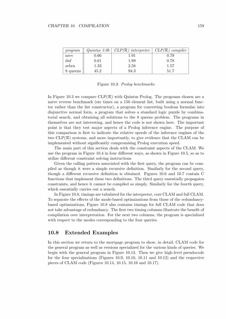
CHAPTER 10. COMPILATION 159
program Quintus 3.0b CLP(R) interpreter CLP(R) compilernrev 0.66 1.91 0.79dnf 0.61 1.89 0.78zebra 1.33 2.58 1.578 queens 45.2 94.3 51.7
Figure 10.3: Prolog benchmarks
In Figure 10.3 we compare CLP(R) with Quintus Prolog. The programs chosen are anaive reverse benchmark (six times on a 150 element list, built using a normal func-tor rather than the list constructor), a program for converting boolean formulae intodisjunctive normal form, a program that solves a standard logic puzzle by combina-torial search, and obtaining all solutions to the 8 queens problem. The programs inthemselves are not interesting, and hence the code is not shown here. The importantpoint is that they test major aspects of a Prolog inference engine. The purpose ofthis comparison is first to indicate the relative speeds of the inference engines of thetwo CLP(R) systems, and more importantly, to give evidence that the CLAM can beimplemented without significantly compromising Prolog execution speed.
The main part of this section deals with the constraint aspects of the CLAM. Weuse the program in Figure 10.4 in four different ways, as shown in Figure 10.5, so as toutilize different constraint solving instructions
Given the calling pattern associated with the first query, the program can be com-piled as though it were a simple recursive definition. Similarly for the second query,though a different recursive definition is obtained. Figures 10.6 and 10.7 contain Cfunctions that implement these two definitions. The third query essentially propagatesconstraints, and hence it cannot be compiled so simply. Similarly for the fourth query,which essentially carries out a search.
In Figure 10.8, timings are tabulated for the interpreter, core CLAM and full CLAM.To separate the effects of the mode-based optimizations from those of the redundancy-based optimizations, Figure 10.8 also contains timings for full CLAM code that doesnot take advantage of redundancy. The first two timing columns illustrate the benefit ofcompilation over interpretation. For the next two columns, the program is specializedwith respect to the modes corresponding to the four queries.
10.8 Extended Examples
In this section we return to the mortgage program to show, in detail, CLAM code forthe general program as well as versions specialized for the various kinds of queries. Webegin with the general program in Figure 10.13. Then we give high-level pseudocodefor the four specializations (Figures 10.9, 10.10, 10.11 and 10.12) and the respectivepieces of CLAM code (Figures 10.14, 10.15, 10.16 and 10.17).

CHAPTER 10. COMPILATION 160
mortgage(P, T, I, R, B) :-T > 1,T1 = T - 1,P >= 0,P1 = P * I - R,mortgage(P1, T1, I, R, B).
mortgage(P, T, I, R, B) :-T = 1,B = P * I - R.
Figure 10.4: Program for reasoning about mortgage repayments
Q1 : ?- mortgage(100000, 360, 1.01, 1025, B).Q2 : ?- mortgage(P, 360, 1.01, 1025, 12625.9).Q3 : ?- R > 0, B >= 0, mortgage(P, 360, 1.01, R, B).Q4 : ?- 0 <= B, B <= 1030, mortgage(100000, T, 1.01, 1030, B).
Figure 10.5: Four queries for the mortgage program
double mg1(p, t, i, r)double p, t, i, r;if (t == 1.0) return (p*i - r);else if (t > 1.0 && p >= 0.0)
return mg1(p*i - r, t - 1.0, i, r);else exit(1);
Figure 10.6: C function for Q1

CHAPTER 10. COMPILATION 161
double mg2(t, i, r, b)double t, i, r, b;double p;if (t == 1.0) return ((b + r)/i);else if (t > 1.0)
p = (mg2(t - 1.0, i, r, b) + r)/i;if (p >= 0.0) return p; else exit(1);
else exit(1);
Figure 10.7: C function for Q2
CLP(R) CLP(R) CLP(R) full CLAM CLP(R) Cquery interpreter core CLAM but no redundancy full CLAM programQ1 0.10 0.05 0.0042 0.0042 0.0010Q2 2.08 1.78 0.0054 0.0054 0.0016Q3 2.35 1.84 1.05 0.0700 n/aQ4 4.20 2.05 1.78 0.0640 n/a
Figure 10.8: Timings for Mortgage program

CHAPTER 10. COMPILATION 162
mortgage(P,T,I,R) =if T > 1T1 ← T − 1if P ≥ 0P1 ← P ∗ I −Rreturn mortgage(P1,T1,I,R)
else failelse if T = 1
return P ∗ I −Relse fail
?-P ← 100000T ← 360I ← 1.01R← 1025B ← mortgage(P,T,I,R)
Figure 10.9: High-level pseudocode: mortgage specialized for Q1
mortgage(T,I,R,B) :-if T > 1T1 ← T − 1P1 ← mortgage(T1,I,R,B).if P ≥ 0return P
eqn( P1 = P * I - R )else fail
else if T = 1V1 ← (B +R)/Ireturn V1
else fail
?-T ← 360I ← 1.01R← 1025B ← 12625.9P ← mortgage(T,I,R,B)
Figure 10.10: High-level pseudocode: mortgage specialized for Q2
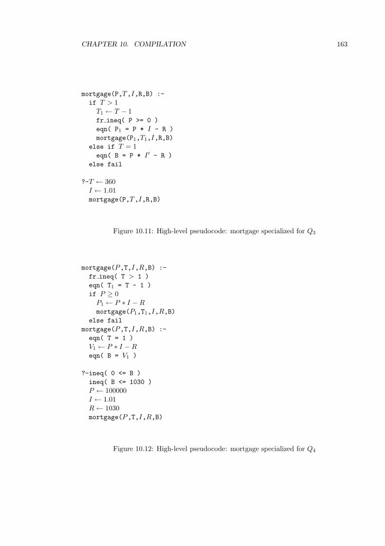
CHAPTER 10. COMPILATION 163
mortgage(P,T,I,R,B) :-if T > 1T1 ← T − 1fr ineq( P >= 0 )eqn( P1 = P * I - R )mortgage(P1,T1,I,R,B)
else if T = 1eqn( B = P * I ′ - R )
else fail
?-T ← 360I ← 1.01mortgage(P,T,I,R,B)
Figure 10.11: High-level pseudocode: mortgage specialized for Q3
mortgage(P,T,I,R,B) :-fr ineq( T > 1 )eqn( T1 = T - 1 )if P ≥ 0P1 ← P ∗ I −Rmortgage(P1,T1,I,R,B)
else failmortgage(P,T,I,R,B) :-eqn( T = 1 )V1 ← P ∗ I −Reqn( B = V1 )
?-ineq( 0 <= B )ineq( B <= 1030 )P ← 100000I ← 1.01R← 1030mortgage(P,T,I,R,B)
Figure 10.12: High-level pseudocode: mortgage specialized for Q4

CHAPTER 10. COMPILATION 164
mg try mg1, 5trust mg2
mg1 initpf -1addpf val + #Tsolve gt0initpf 1addpf val -1, #Taddpf var + #tmp1solve eq0initpf 0addpf val + #Psolve ge0mult Vvv #tmp3, #P, #Iinitpf 0addpf val + #Raddpf val -1, #tmp3addpf var + #tmp2solve eq0getvar #P, #tmp2getvar #T, #tmp1jump mg
mg2 gettnum 1, #Tmult Vvv #tmp1, #P, #Iinitpf 0addpf val + #Raddpf val -1, #tmp1addpf val + #Bsolve eq0proceed
Figure 10.13: Core CLAM code for general mortgage program

CHAPTER 10. COMPILATION 165
mg subcf #T, 1, #tmpjgtf #tmp, mg1jeqf #tmp, mg2fail
mg1 mvf #tmp, #Tjgef #P, contfail
cont mulf #P, #I, #tmpsubf #tmp, #R, #Pjump mg
mg2 mulf #P, #I, #tmpsubf #tmp, #R, #Bproceed
Figure 10.14: Extended CLAM code for mortgage program, specialized for Q1
mg save 0subf #T, 1, #tmpjgtf #tmp, mg1jeqf #tmp, mg2fail
mg1mvf #tmp, #Tcallp mgaddf #P, #R, #tmpdivf #tmp, #I, #Pjgtf #P, cont1jeqf #P, cont1fail
cont1restoreproceed
mg2addf #R, #B, #tmpdivf #tmp, #I, #Prestoreproceed
Figure 10.15: Extended CLAM code for mortgage program, specialized for Q2

CHAPTER 10. COMPILATION 166
mg subcf #T, 1, #tmpjgtf #tmp, mg1jeqf #tmp, mg2fail
mg1 subcf #T, 1, #Tjgtf #T, cont1fail
cont1 initpf 0addpf val + #Psolve no add ge0initpf 0addpf fp val #I, #Paddpf val - #Rsolve no fail eq #tmp3getvar #P, #tmp3jump mg
mg2 subcf #T, 1, #tmp4jeqf #tmp4, cont2fail
cont2 subfc 0, #I, #tmp2initpf 0addpf val + #Raddpf fp val #tmp2, #Paddpf val + #Bsolve eq0proceed
Figure 10.16: Extended CLAM code for mortgage program, specialized for Q3

CHAPTER 10. COMPILATION 167
mgtry mg1, 9trust mg2
mg1initpf -1addpf val + #Tsolve no add gt0initpf -1addpf val + #Tsolve no fail eq #tmpjgtf #P, cont1jeqf #P, cont1fail
cont1mulf #P, #I, #tmp1subf #tmp1, #R, #Pgettvar #T, #tmpjump mg
mg2initpf -1addpf val + #Tsolve eq0mulf #P, #I, #tmp1subf #tmp1, #R, #tmp2initpf fp #tmp2addpf val - #Bsolve eq0proceed
Figure 10.17: Extended CLAM code for mortgage program, specialized for Q4
Chapter 11
Efficient Implementation of Elf
The objective of this chapter is to give some specific proposals for an efficient imple-mentation of Elf, based on the ideas and techniques presented in the rest of this thesis.Many of the comments made about Elf will also be applicable to λProlog. This chapterdoes not describe any existing implementation, but the prescriptions are based heavilyon the empirical study described in Section 5.6.
We begin by discussing the problem of implementing CLP languages with equalityconstraints on typed λ-expressions. Then we give an overview of higher-order unifi-cation, the standard technique for solving these constraints for the simply-typed λ-calculus, as described by Huet [76], and extended by Elliott to dependent types [50].We restrict the constraint problem as described in Chapter 5 to avoid the hardest cases,and thus describe a modified form of higher-order unification, and show how this fitsin with the methodology for managing hard constraints as described in Chapter 8. Fi-nally, based on empirical evidence we describe how to prioritize constraint solving sothat the frequent simple cases are solved with relatively low overhead.
11.1 Higher-Order Unification
To understand the relevant points of higher-order unification, we need to take anotherlook at first-order unification. Recall that the Robinson unification algorithm for first-order terms is usually formulated as a set of rewrite rules on a set of disagreementpairs, each of which is a pair of terms, and a most general substitution for the variablesis required making the terms in each such pair equal. This is called a most generalunifier (mgu), which is guaranteed to exist if the equality constraints are satisfiable,and to be unique modulo variable renaming. Note that the mgu is a solved form for theset of equality constraints in the sense that it is a representation of certain eliminablevariables as terms possibly including non-eliminable, or parametric variables.
Higher-order unification can be described in a similar way, but there are compli-cations. The notion of uniqueness for solutions is now modulo not only re-namingexistential variables, but also αβη-convertibility. As we have already discussed, in thisrespect most general unifiers do not exist. If we require answers in solved form as
168

CHAPTER 11. EFFICIENT IMPLEMENTATION OF ELF 169
described above, the best we can do is an algorithm that will enumerate the possiblyinfinite set of pre-mgus. That is, each solution will be an instance of at least one ofthe unifiers. As has already been mentioned in Chapter 5, this has unpleasant practi-cal consequences. However, if we relax the solved form requirement, a pre-unificationalgorithm is available. If a set of constraints is satisfiable, the algorithm terminateswith a solution in the usual form, together with some equality constraints that do notconform to the solved form, but are known to be satisfiable. For reasons that will bemade clear below, these constraints are called Flex − Flex pairs. Thus unification isnow, at a pragmatic level, more like general constraint solving, since a store is neededto maintain the set of substitutions and Flex-Flex pairs. At times, Flex-Flex pairs willdisappear in the forward direction as more information becomes available, and thenhave to be restored on backtracking. Note that these constraints are not “hard” or“delayed” in the usual sense, as their satisfiability is guaranteed rather than assumed,but many of the same implementation issues arise.
The pre-unification problem is still undecidable, and so this algorithm still may notterminate when no solution exists. This is because it is still non-deterministic, requiringa search through possibly infinite sets of unifiers for some sub-problem, for one thatcorresponds to a solution of another part. If none exists, the search may be infinite, butif a solution does exist, it will eventually be found. This problem arises because of someother kinds of disagreement pairs, the so-called Flex− Rigid pairs, and Flex−Gvarpairs, a special case of Flex − Flex pairs. (and of course their symmetric cases). Toillustrate these situations, consider two constraints c1 and c2, where c1 has an infiniteset of pre-mgus, c2 has a finite one, but c1 and c2 are jointly unsatisfiable. The pre-unification algorithm will choose the first solution to c1, and then search through thesolutions to c2 to find one that is compatible. None will be found, and the same willhappen for the second solution to c1, and the third, and so on. The procedure doesn’tterminate, since it never runs out of solutions to c1 to try, and none are consistent withany of the solutions to c2.
In Chapter 5 it was argued that Flex-Rigid and Flex-Gvar pairs will occur ratherrarely, and in Section 5.6 the empirical results bore this out, as they occurred in onlyone of the examples. Furthermore, it was shown that these can be deferred until theybecome simpler through additional information becoming available. This means thatwe can classify them as hard constraints, and delay them until they are simplifiedsufficiently to avoid this problem. Then unification itself will always terminate, but ofcourse the usual potential problems of search control that are associated with delay areintroduced.
There is an additional complication, in that Flex-Flex pairs can actually give riseto hard constraints when further information becomes available. This will be discussedfurther in Section 11.2.
It should be noted that Elliott’s extension of Huet’s pre-unification algorithm, andPfenning’s extension of Miller’s algorithm for the Lλ subset are incomparable in terms ofwhich disagreement pairs they actually solve. This is summarized in the set inclusiondiagram in Figure 11.1. Of course neither of them solve Flex-Flex pairs, or for themost part Flex-Gvar pairs, although the latter can be solved by the Miller/Pfenning

CHAPTER 11. EFFICIENT IMPLEMENTATION OF ELF 170
Huet / Elliott Miller / Pfenning
Flex-Rigid Gvar-Gvar
Figure 11.1: Comparison of solutions in Huet’s and Miller’s algorithms
algorithm as an optimization for certain special cases. We should also note that in thisdiscussion the Flex case does not include the Gvar case, unlike in Huet’s usage.
Now, let us list the various forms fo terms in disagreement pairs. For higher-orderunification for dependent types, the interested reader is referred to [51] — we restrictthe discussion to the simply-typed subset. An Evar is an existential variable, and aUvar is a temporary constant introduced by pi-quantification. An Evar E is said todepend on a Uvar x in a goal if E is bound inside the scope of x in the goal.
• FlexFM1M2 · · ·Mn, n ≥ 0 where F is an Evar and the Mi are terms, and the Gvarconditions below are not satisfied.
• GvarFx1x2 · · ·xm, 0 ≤ m ≤ n where F is an Evar, the xi are Uvars, F does not dependon any xi, and the xi are all distinct.
• RigidfM1M2 · · ·Mn, n ≥ 0 where f is a constant or a Uvar and the Mi are terms.
Note that, to simplify the discussion, types have been omitted, and the the otherclasses of disagreement pairs have been omitted since they are dealt with by straight-forward recursive unifications.
11.2 Hard Constraints
In this section, our aim is to describe the management of hard constraints in Elf in termsof the framework developed in Chapter 8. We will work towards this goal somewhatgradually.

CHAPTER 11. EFFICIENT IMPLEMENTATION OF ELF 171
Core Elf Unification TableGvar Flex Rigid
Gvar unifyFlex delay delayRigid unify delay unify
Figure 11.2: Core unification table for Elf
The situation is described in Figure 11.2.Because a Flex-Flex pair, which is not a hard constraint, can lead to a hard con-
straint we include Flex-Flex pairs in the wakeup system. Hence, ideally, we need fivewakeup degrees in addition to awakened, These are for Flex-Flex, Flex-Rigid, Rigid-Flex, Flex-Gvar, and Gvar-Flex. We note that it is not desirable to combine symmetriccases. This is because the transitions of the two sides of the equation depend on thebinding of different variables, and we need to distinguish them for efficient implemen-tation.
The transitions between these three forms of expressions that we need to considerare as follows. Note that we do not consider leading abstractions.
1. Flex ⇒ RigidThe head F is bound to
λx1 · · ·λxk. gN1 · · ·Nm
where g is a constant or a Uvar and the Ni are terms. The resulting Rigid termwill, of course, be of the form
gP1 · · ·Pl.
2. Gvar ⇒ RigidSame as Flex ⇒ Rigid.
3. Flex ⇒ Gvar
(a) All of the arguments are bound to universal variables, such that the partialpermutation property holds. (This is very unlikely, and expensive to checkfor, so it has not been implemented to date).
(b) The head F is bound to
λx1 · · ·λxk. Gy1 · · · ym
where G is an existential variable, each yj is either a Uvar or one of the xi,and the resulting term is a Gvar. That is,
Gz1 · · · zlsuch that the zi are all distinct Uvars, and G does not depend on any ofthem.

CHAPTER 11. EFFICIENT IMPLEMENTATION OF ELF 172
4. Gvar ⇒ FlexThe head F is bound to
λx1 · · ·λxk. GN1 · · ·Nm
where G is a an existential variable and the Ni are terms, such that the Gvarcriteria are now violated. The resulting Flex term will be of the form
GP1 · · ·Pl.
Notice that the above transitions admit the possibility of cycles. A Flex termcan turn into a Gvar term when more information becomes available, and with stillmore information may turn back into a Flex term, all without backtracking. Thismakes the wakeup system cyclic, as shown in Figure 11.3. Note that the two arcsshown using a thinner line correspond to the case that is expensive and unlikely, andmight be omitted. We describe the generic wakeup conditions in symmetric pairs, toavoid notational clutter, and ignore the term that does not change in each pair. Thelanguage in our description of the degrees and wakeup conditions is different to thatused in Chapter 8, to make it more intuitive in this context.
11.3 Easy Cases of Constraints
Finally we consider details of the actual implementation of higher-order unification,given the empirical data of section 5.6. Recall that that most unification was eithersimple assignment or first-order (Herbrand) unification, around 95%, averaged overall examples. Similarly, substitution was the substitution of parameters for λ-boundvariables in about 95% of the cases. The remaining 5% were substitution of constants,variables, or compound terms for bound variables.
The aim is to find a representation for Elf terms, substitutions and constraints thatis suitable for the general problem at hand but is especially suited to the frequentsimple cases. The obvious representation is that corresponding to first-order abstractsyntax: a DAG with special nodes for application, abstraction etc. This is problematicbecause of the frequency of the Rigid-Rigid case in unification — remembering thatunification avoided by indexing represents otherwise uncounted instances of Rigid-Rigidunification.
Representing application in the obvious way, as shown in the example in Figure11.4, is particularly problematic. The term shown in the example is FM1M2M3M4.Consider the problem of classifying a disagreement pair. The classifications are mostlybased on the nature of the head: in particular whether it is bound to a constant ornot. Furthermore, in the frequently occurring Rigid-Rigid case, it is necessary to knowwhich constant: as the pair is only decomposed into argument pairs if the heads areidentical. In this representation, obtaining information about the head is too expensive.It is necessary to have the head immediately accessible, and then the arguments mightas well be a list. This representation, for the same example, is shown in Figure 11.5.

CHAPTER 11. EFFICIENT IMPLEMENTATION OF ELF 173
W
F-F
F-G G-FF-R R-F
ω ω
ω ω
ωω
ω
ωω
ω
ω ω
1 2
3 45 6
7 89 10
11 12
(G-G, R-R, G-R, R-G)
ωω
ωωω
ω
13 14
15 16
17 18
F FM1M2 · · ·Mn
G Fxφ1xφ2 · · ·xφm
R fM1M2 · · ·Mn
F -> R (ω1, ω2, ω13, ω14, ω15, ω16) F = λx1 · · ·λxk. gN1 · · ·Nm
F -> G (ω5, ω6) M1 = x1 ∧ · · · ∧Mn = xn
∧ Gvar(Fx1 · · ·xn)F -> G (ω3, ω4, ω11, ω12, ω17, ω18) F = λx1 · · ·λxk. Gy1 · · · ym
∧ (λx1 · · ·λxk. Gy1 · · · ym)M1 · · ·Mn →M ′
∧ Gvar(M ′)G -> R (ω9, ω10) F = λx1 · · ·λxk. gN1 · · ·Nm
G -> F (ω7, ω8) F = λx1 · · ·λxk. GN1 · · ·Nm
∧ (λx1 · · ·λxk. GN1 · · ·Nm)M1 · · ·Mn →M ′
∧ ¬Gvar(M ′)
Figure 11.3: Wakeup system for Elf

CHAPTER 11. EFFICIENT IMPLEMENTATION OF ELF 174
@
@
@
@
M
M
M
M
1
2
3
4
F
Figure 11.4: Conventional term representation for Elf
M1
M2
M3
M 4
F
nil
Figure 11.5: Functor/Arguments term representation for Elf

CHAPTER 11. EFFICIENT IMPLEMENTATION OF ELF 175
Notice that this representation also makes it easier to make use of clause indexing onrigid term heads.
Note that this functor/argument representation can be problematic when the head isflexible, since it can then be bound to an expression which requires some normalization,producing a new head, and the old one needs to be stored for backtracking in someway. These complications are outbalanced by the efficiency improvement for the simplecases.
Note also that this discussion hinges on rigid terms being in close correspondencewith constructed terms in Prolog. The constant head is the functor, and the remain-ing terms are the arguments. There is then also a close correspondence with Prologindexing. In short, Prolog unification is an important special case of Elf equality con-straints, and this fact affects the representation of application especially. We concludethat functor/argument representation, as was in fact used in Nadathur’s original im-plementation of λProlog up to LP2.7, is an essential optimization for a λProlog or Elfimplementation.
11.4 Other Implementation Issues
A number of other representation and implementation issues arise from a study of theempirical data in Section 5.6. Here we make a number of brief comments on thoseissues.
• Term ComparisonIn principle, an important part of term comparison in these languages is the testfor α-convertibility. The Duke representation proposal [127] suggests a De Bruijn[38] representation of terms for this reason. While that suggestion may well beappropriate, we should note that the empirical study showed the comparison oftwo abstractions to be a rare occurrence, and hence it should be probably not beallowed to determine the choice of term representation.
• Substitution and AbstractionThe obvious way to handle substitutions is to produce explicitly the new term.However, this is time-consuming since the function applied must be traversed,and space consuming, since multiple copies of a large term may have to be made.However, other representations of substitutions tend to be complicated in general.This is not the case for substitutions of Uvars. Furthermore, most of the substi-tutions actually performed are Uvars, and these are frequently abstracted over aswell. Abstraction is typically less expensive when substitutions are not actuallymade, but represented in some explicit way. The Duke proposal advocates usingembellished environments to represent substitutions efficiently.
• Building DeductionsBuilding deductions is expensive. However, it need only be done when the overall

CHAPTER 11. EFFICIENT IMPLEMENTATION OF ELF 176
deduction is requested by the user, or when a deduction is needed for further com-putation. In this sense goals that do not use partial deductions for computationlead to behavior that is closer to that of λProlog.
• TypesType computations in Elf are a significant part of the overall work done, andeliminating redundant type computations is likely to be important.
• Extended Occurs CheckThe occurs check is particularly important in λProlog and Elf, as programs quitecommonly depend on it to run correctly. However, even local analysis of rulescan be used to avoid many uses of it in most Elf programs. This is because headsof rules are typically linear, so that each variable occurs only once, and thus theoccurs check can largely be avoided when these variables are bound. Likewise thedependency check can often be avoided.

Part IV
Conclusions
177

Chapter 12
Conclusions
The main contribution of this thesis has been to demonstrate the practicality of con-straint logic programming by using CLP(R) as a case study. It has been shown thatpaying close attention to the relationship between programming methodology, languagedesign and efficient implementation can enable us to design CLP systems that have theexpressive power to provide leverage to programmers yet be efficiently implementable.
The specific contributions can be summarized as follows:
• An understanding of CLP(R) and Elf programming methodology. This consistsof an understanding of both static program structure and the empirical aspectsof program execution.
• A discipline for dealing with hard constraints by delaying them at runtime.
• A strategy for structuring constraint solvers to take advantage of frequently oc-curring simple cases of constraints.
• An understanding of the problems of adapting constraint solvers to the opera-tional model of CLP by making them incremental.
• Design of suitable data structures for incremental constraint solving.
• A strategy and abstract machine design for compiling CLP(R) based on thecentral data structure of the constraint solver.
• A strategy for making use of highly optimizing compilation of CLP(R) based onglobal program analysis and multiple program specialization.
The broad applicability of the techniques developed here has been demonstratedthrough a second case study. Elf is superficially almost totally unlike CLP(R), exceptfor being essentially a CLP language. However, when viewed in the way that this thesisadvocates, the two languages, and to varying extents the various other CLP languages,can be seen to be strongly related not only conceptually, but also pragmatically. Thisrelationship is more obvious for most of the other CLP languages discussed, and theparallels are even stronger. The ideas and techniques in this thesis have been validated
178
CHAPTER 12. CONCLUSIONS 179
in practice to a considerable degree. In particular, the CLP(R) systems have been usedfor a substantial number of non-trivial applications, as described in Chapter 4.
There is still much work to be done in the practical aspects of Constraint LogicProgramming. To mention just a few important areas of research:
• Incremental constraint solving for other domains, and for wider class of con-straints in the usual domains.
• Practical, highly optimizing compilers for CLP(R) and other languages.
• Control and usability issues in language design.
• Pursuit of other application areas.
• A program debugging methodology to accommodate search for causes of failurethrough constraint unsatisfiability.
It is hoped that this thesis, however, provides a practical guide for future developersof CLP systems.

Appendix A
Electrical Engineering Programs
A.1 Circuit Solver
This program carries out a steady state phasor analysis of RLC circuits. It is calledthrough the predicate circuit solve() which has as arguments
• the angular frequency for the analysis.
• the component list.
• the list of nodes which are to be ‘grounded’ — otherwise all voltages are relative.
• the ‘Selection’ list — a list of nodes for which computed information is to beprinted.
The circuit is defined by a list of components. Each component is described by thecomponent type, name, value and the nodes to which it is connected. The componenttype is used to determine the component characteristics.
circuit_solve(W, L, G, Selection) :-get_node_vars(L, NV),solve(W, L, NV, Handles, G),format_print(Handles, Selection).
get_node_vars([[Comp, Num, X, Ns]|Ls], NV) :-get_node_vars(Ls, NV1),insert_list(Ns, NV1, NV).
get_node_vars([], []).
insert_list([N|Ns], NV1, NV3) :-insert_list(Ns, NV1, NV2),insert(N, NV2, NV3).
insert_list([], NV, NV).
insert(N, [[N, V, I]|NV1], [[N, V, I]|NV1]).
180

APPENDIX A. ELECTRICAL ENGINEERING PROGRAMS 181
insert(N, [[N1, V, I]|NV1], [[N1, V, I]|NV2]) :-insert(N, NV1, NV2).
insert(N, [], [[N, V, c(0, 0)]]).
solve(W, [X|Xs], NV, [H|Hs], G) :-addcomp(W, X, NV, NV1, H),solve(W, Xs, NV1, Hs, G).
solve(W, [], NV, [], G) :-zero_currents(NV),ground_nodes(NV, G).
zero_currents([[N, V, c(0, 0)]|Ls]) :-zero_currents(Ls).
zero_currents([]).
ground_nodes(Vs, [N|Ns]) :-ground_node(Vs, N),ground_nodes(Vs, Ns).
ground_nodes(Vs, []).ground_node([[N, c(0, 0), I]|Vs], N).ground_node([[N1, V, I]|Vs], N) :-
ground_node(Vs, N).
%% The following rules deal with two-terminal components.%addcomp(W, [Comp2, Num, X, [N1, N2]], NV, NV2,
[Comp2, Num, X, [N1, V1, I1], [N2, V2, I2]]):-c_neg(I1, I2),iv_reln(Comp2, I1, V, X, W),c_add(V, V2, V1),subst([N1, V1, Iold1], [N1, V1, Inew1], NV, NV1),subst([N2, V2, Iold2], [N2, V2, Inew2], NV1, NV2),c_add(I1, Iold1, Inew1),c_add(I2, Iold2, Inew2).
%% Voltage/current relationships for two-terminal components.%iv_reln(resistor, I, V, R, W) :-
c_mult(I, c(R, 0), V).iv_reln(voltage_source, I, V, V, W).iv_reln(isource, I, V, I, W).iv_reln(capacitor, I, V, C, W) :-
c_mult(c(0, W*C), V, I).iv_reln(inductor, I, V, L, W) :-
c_mult(c(0, W*L), I, V).iv_reln(connection, I, c(0, 0), L, W).iv_reln(open, c(0, 0), V, L, W).

APPENDIX A. ELECTRICAL ENGINEERING PROGRAMS 182
iv_reln(diode, I, V, D, W) :-diode(D, I, V).
%% Three rules per diode type.%diode(in914, c(I, 0), c(V, 0)) :-
V < -100, DV = V + 100, I = 10*DV.diode(in914, c(I, 0), c(V, 0)) :-
V >= -100, V < 0.6, I = 0.001*V.diode(in914, c(I, 0), c(V, 0)) :-
V >= 0.6, DV = V - 0.6, I = 100*DV.
%% The following rules deal with transistors.%addcomp(W, [transistor, Num, X, [N1, N2, N3]], NV, NV3,
[transistor, Num, X, [N1, V1, I1],[N2, V2, I2], [N3, V3, I3]]):-
transistor(X, R, Gain),c_add(I1, I3, IT),c_neg(I2, IT),c_add(Vin, V2, V1),c_mult(I1, c(R, 0), Vin),c_mult(I1, c(Gain, 0), I3),subst([N1, V1, Iold1], [N1, V1, Inew1], NV, NV1),subst([N2, V2, Iold2], [N2, V2, Inew2], NV1, NV2),subst([N3, V3, Iold3], [N3, V3, Inew3], NV2, NV3),subst([N4, V4, Iold4], [N4, V4, Inew4], NV3, NV4),c_add(I1, Iold1, Inew1),c_add(I2, Iold2, Inew2),c_add(I3, Iold3, Inew3),c_add(I4, Iold4, Inew4).
% We need one fact for each kind of transistor we wish to consider.
transistor(bc108, 1000, 100).
%% The following rule deals with transformers.%addcomp(W, [transformer, Num, X, [N1, N2, N3, N4]], NV, NV4,
[transformer, Num, X, [N1, V1, I1], [N2, V2, I2],[N3, V3, I3], [N4, V4, I4]]):-
c_neg(I1, I2),c_neg(I3, I4),c_add(Vin, V2, V1),c_add(Vout, V4, V3),c_mult(Vout, c(X, 0), Vin),

APPENDIX A. ELECTRICAL ENGINEERING PROGRAMS 183
c_mult(I1, c(X, 0), I4),subst([N1, V1, Iold1], [N1, V1, Inew1], NV, NV1),subst([N2, V2, Iold2], [N2, V2, Inew2], NV1, NV2),subst([N3, V3, Iold3], [N3, V3, Inew3], NV2, NV3),subst([N4, V4, Iold4], [N4, V4, Inew4], NV3, NV4),c_add(I1, Iold1, Inew1),c_add(I2, Iold2, Inew2),c_add(I3, Iold3, Inew3),c_add(I4, Iold4, Inew4).
subst(X, Y, [X|L1], [Y|L1]).subst(X, Y, [Z|L1], [Z|L2]) :-
subst(X, Y, L1, L2).
%% These rules define complex arithmetic.%
c_mult(c(Re1, Im1), c(Re2, Im2), c(Re3, Im3)) :-Re3 = Re1*Re2 + -1*Im1*Im2,Im3 = Re1*Im2 + Re2*Im1.
c_add(c(Re1, Im1), c(Re2, Im2), c(Re3, Im3)) :-Re3 = Re1 + Re2,Im3 = Im1 + Im2.
c_neg(c(Re, Im), c(Re1, Im1)) :-Re1 = -Re, Im1 = -Im .
c_eq(c(Re1, Im1), c(Re2, Im2)) :-Re1 = Re2, Im1 = Im2 .
c_real(c(Re, Im), Re).c_imag(c(Re, Im), Im).
% format_print(H, Selection) --- Print out node information.
A.2 Transistor Circuit Analysis and Design
This program solves transistor amplifier design and analysis problems, and D.C. circuitanalysis problems involving transistors, diodes and capacitors. The first main goal,used for dc analysis of circuits, is
?- dc_analysis(Vcc1, Vcc2, Circuit).
The parameters are two (optional) source voltages which will ensure that the node cc1is at voltage Vcc1, similarly for cc2, and a circuit description in the following form: alist of elements each of which is a list containing four elements, the component type, the

APPENDIX A. ELECTRICAL ENGINEERING PROGRAMS 184
component name, the data for the component, and a list of nodes that the componentconnects.
The second main goal, used for transistor amplifier design and analysis, is
?- full_analysis(Vcc1, Vcc2, Circuit, In, Out, Type,Stability, Gain, Inresist, Outresist).
The first three parameters are as above. The rest are the input node for the amplifier,the output node for the amplifier, and the type (emitter-follower, common-base) of theamplifier. The final four parameters are design parameters: the stability of collectorcurrents on 50% deviation of Beta values and 10% deviation of Vbe values for thetransistors of the amplifier, the gain of the amplifier, and finally the open-circuit inputresistance and output resistance of the amplifier.
Note that several conventions are followed in this program. In the D.C. case, ca-pacitors are considered to be open circuits. However, for small signal analysis, they areconsidered to be short circuits. Additionally, it is assumed that any amplifier circuittype used for a full analysis appears in the database of circuits and that all componentsused appear in the database of components.
%% Entry Points.%
dc_analysis(Vcc1, Vcc2, Circuit):-choose_circuit(Circuit),solve_dc(mean, Circuit, [n(cc1, Vcc1, [_]),
n(cc2, Vcc2, [_]), n(gnd, 0, [_])],Nodelist, Collector_Currents),
current_solve(Nodelist),print_circuit(Circuit),print_value(Nodelist).
full_analysis(Vcc1, Vcc2, Circuit, In, Out, Type,Stability, Gain, Inresist, Outresist):-
% Choose a circuit template.circuit(Vcc1, Vcc2, Circuit, In, Out, Type),% Construct circuit constraints.solve_dc(mean, Circuit, [n(cc1, Vcc1, [_]),
n(cc2, Vcc2, [_]), n(gnd, 0, [_])],Nodelist, Collector_Currents),
current_solve(Nodelist),% Determine stability constraints.stability(Vcc1, Vcc2, Circuit, Collector_Currents, Stability),% Determine input resistance and gain constraints.solve_ss(Circuit, Collector_Currents,
[n(cc1, 0, [_]), n(cc2, 0, [_]),n(gnd, 0, [_]), n(In, 1, [Iin]),n(Out, Vout, [])], Nodelist2),
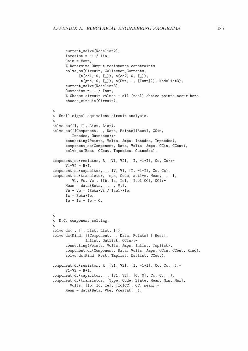
APPENDIX A. ELECTRICAL ENGINEERING PROGRAMS 185
current_solve(Nodelist2),Inresist = -1 / Iin,Gain = Vout,% Determine Output resistance constraintssolve_ss(Circuit, Collector_Currents,
[n(cc1, 0, [_]), n(cc2, 0, [_]),n(gnd, 0, [_]), n(Out, 1, [Iout])], Nodelist3),
current_solve(Nodelist3),Outresist = -1 / Iout,% Choose circuit values - all (real) choice points occur herechoose_circuit(Circuit).
%% Small signal equivalent circuit analysis.%solve_ss([], [], List, List).solve_ss([[Component, _, Data, Points]|Rest], CCin,
Innodes, Outnodes):-connecting(Points, Volts, Amps, Innodes, Tmpnodes),component_ss(Component, Data, Volts, Amps, CCin, CCout),solve_ss(Rest, CCout, Tmpnodes, Outnodes).
component_ss(resistor, R, [V1, V2], [I, -1*I], Cc, Cc):-V1-V2 = R*I.
component_ss(capacitor, _, [V, V], [I, -1*I], Cc, Cc).component_ss(transistor, [npn, Code, active, Mean, _, _],
[Vb, Vc, Ve], [Ib, Ic, Ie], [Icol|CC], CC):-Mean = data(Beta, _, _, Vt),Vb - Ve = (Beta*Vt / Icol)*Ib,Ic = Beta*Ib,Ie + Ic + Ib = 0.
%% D.C. component solving.%solve_dc(_, [], List, List, []).solve_dc(Kind, [[Component, _, Data, Points] | Rest],
Inlist, Outlist, CCin):-connecting(Points, Volts, Amps, Inlist, Tmplist),component_dc(Component, Data, Volts, Amps, CCin, CCout, Kind),solve_dc(Kind, Rest, Tmplist, Outlist, CCout).
component_dc(resistor, R, [V1, V2], [I, -1*I], Cc, Cc, _):-V1-V2 = R*I.
component_dc(capacitor, _, [V1, V2], [0, 0], Cc, Cc, _).component_dc(transistor, [Type, Code, State, Mean, Min, Max],
Volts, [Ib, Ic, Ie], [Ic|CC], CC, mean):-Mean = data(Beta, Vbe, Vcestat, _),

APPENDIX A. ELECTRICAL ENGINEERING PROGRAMS 186
transistor_state(Type, State, Beta, Vbe, Vcesat, Volts,[Ib, Ic, Ie]).
component_dc(transistor, [Type, Code, State, Mean, Min, Max],Volts, [Ib, Ic, Ie], [Ic|CC], CC, minn):-
Min = data(Beta, Vbe, Vcestat, _),transistor_state(Type, State, Beta, Vbe, Vcesat, Volts,
[Ib, Ic, Ie]).component_dc(transistor, [Type, Code, State, Mean, Min, Max],
Volts, [Ib, Ic, Ie], [Ic|CC], CC, maxx):-Max = data(Beta, Vbe, Vcestat, _),transistor_state(Type, State, Beta, Vbe, Vcesat, Volts,
[Ib, Ic, Ie]).component_dc(diode, [Code, State, Vf, Vbreak], Volts, Amps,
Cc, Cc, _):-diode_state(State, Vf, Vreak, Volts, Amps).
%% Diode and transistor states / relationships.%
diode_state(forward, Vf, Vbreak, [Vp, Vm], [I, -1*I]):-% forward biasedVp - Vm = Vf,I >= 0.
diode_state(reverse, Vf, Vbreak, [Vp, Vm], [I, -1*I]):-% reverse biasedVp - Vm < Vf,Vm - Vp < Vbreak,I = 0.
transistor_state(npn, active, Beta, Vbe, _, [Vb, Vc, Ve],[Ib, Ic, Ie]):-
Vb = Ve + Vbe,Vc >= Vb,Ib >= 0,Ic = Beta*Ib,Ie+Ib+Ic = 0.
transistor_state(pnp, active, Beta, Vbe, _, [Vb, Vc, Ve],[Ib, Ic, Ie]):-
Vb = Ve + Vbe,Vc <= Vb,Ib <= 0,Ic = Beta*Ib,Ie+Ib+Ic = 0.
transistor_state(npn, saturated, Beta, Vbe,Vcesat, [Vb, Vc, Ve], [Ib, Ic, Ie]):-
Vb = Ve + Vbe,Vc = Ve + Vcesat,Ib >= 0,

APPENDIX A. ELECTRICAL ENGINEERING PROGRAMS 187
Ic >= 0,Ie+Ib+Ic = 0.
transistor_state(pnp, saturated, Beta, Vbe,Vcesat, [Vb, Vc, Ve], [Ib, Ic, Ie]):-
Vb = Ve + Vbe,Vc = Ve + Vcesat,Ib <= 0,Ic <= 0,Ie+Ib+Ic = 0.
transistor_state(npn, cutoff, Beta, Vbe,Vcesat, [Vb, Vc, Ve], [Ib, Ic, Ie]):-
Vb <= Ve + Vbe,Ib = 0,Ic = 0,Ie = 0.
transistor_state(pnp, cutoff, Beta, Vbe,Vcesat, [Vb, Vc, Ve], [Ib, Ic, Ie]):-
Vb >= Ve + Vbe,Ib = 0,Ic = 0,Ie = 0.
%% Component connections.%connecting([], [], [], List, List).connecting([P|PR], [V|VR], [I|IR], Inlist, Outlist):-
connect(P, V, I, Inlist, Tmplist),connecting(PR, VR, IR, Tmplist, Outlist).
connect(P, V, I, [], [n(P, V, [I])]) :-!.
connect(P, V, I, [n(P, V, Ilist) | Rest], [n(P, V, [I|Ilist])|Rest]) :-!.
connect(P, V, I, [A|Rest], [A|Newrest]) :-connect(P, V, I, Rest, Newrest).
%% Stability analysis.%stability(Vcc1, Vcc2, Circuit, CollectorCurrents, Stability):-
solve_dc(minn, Circuit, [n(cc1, Vcc1, [_]),n(cc2, Vcc2, [_]), n(gnd, 0, [_])],Nodelist1, MinCurrents),
current_solve(Nodelist1),solve_dc(maxx, Circuit , [n(cc1, Vcc1, [_]),
n(cc2, Vcc2, [_]), n(gnd, 0, [_])],Nodelist2, MaxCurrents),
current_solve(Nodelist2),

APPENDIX A. ELECTRICAL ENGINEERING PROGRAMS 188
calculate(MinCurrents, MaxCurrents,CollectorCurrents, Stability).
calculate(MinCurrents, MaxCurrents, CollectorCurrents, Stability):-cal(MinCurrents, MaxCurrents, CollectorCurrents, Percents),maxi(Percents, 0, Stability).
cal([Min|Rin], [Max|Rax], [Ic|Rc], [Pc|Rpc]):-Pc = max(Ic-Min, Max-Ic),cal(Rin, Rax, Rc, Rpc).
cal([], [], [], []).
maxi([N1|R], N2, P):-M = max(N1, N2),maxi(R, M, P).
maxi([], P, P).
current_solve([]).current_solve([n(_, _, L) | Rest]) :-
kcl(L),current_solve(Rest).
print_value([]).print_value([n(P, V, I) | Rest]) :-
printf("% at % %\n", [P, V, I]),print_value(Rest).
print_circuit([]).print_circuit([[Comp, Name, Data, Points] | Rest]) :-
printf(" % at % %\n", [Comp, Name, Data]),print_circuit(Rest).
sum([X|T], Z) :-X+P = Z,sum(T, P).
sum([], 0).
kcl(L) :-sum(L, 0).
%% Choose circuit values.%choose_circuit([[Component_type, _, Data, _] | RestofCircuit]):-
choose_component(Component_type, Data),choose_circuit(RestofCircuit).
choose_circuit([]).
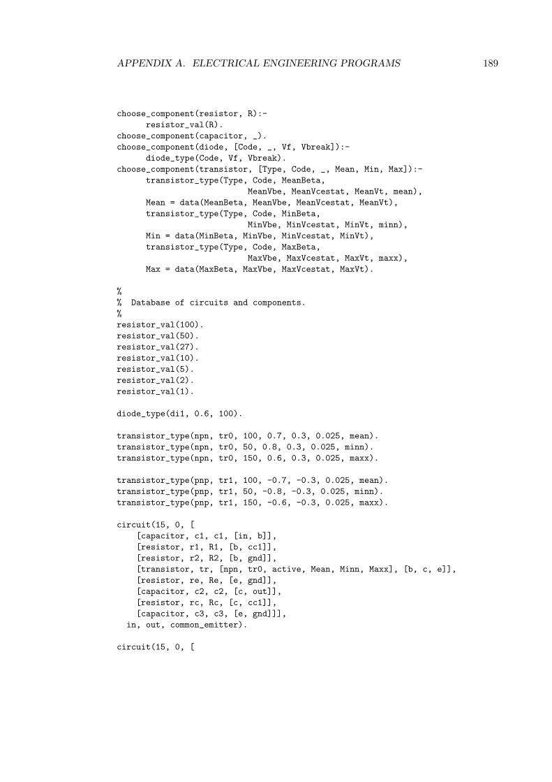
APPENDIX A. ELECTRICAL ENGINEERING PROGRAMS 189
choose_component(resistor, R):-resistor_val(R).
choose_component(capacitor, _).choose_component(diode, [Code, _, Vf, Vbreak]):-
diode_type(Code, Vf, Vbreak).choose_component(transistor, [Type, Code, _, Mean, Min, Max]):-
transistor_type(Type, Code, MeanBeta,MeanVbe, MeanVcestat, MeanVt, mean),
Mean = data(MeanBeta, MeanVbe, MeanVcestat, MeanVt),transistor_type(Type, Code, MinBeta,
MinVbe, MinVcestat, MinVt, minn),Min = data(MinBeta, MinVbe, MinVcestat, MinVt),transistor_type(Type, Code, MaxBeta,
MaxVbe, MaxVcestat, MaxVt, maxx),Max = data(MaxBeta, MaxVbe, MaxVcestat, MaxVt).
%% Database of circuits and components.%resistor_val(100).resistor_val(50).resistor_val(27).resistor_val(10).resistor_val(5).resistor_val(2).resistor_val(1).
diode_type(di1, 0.6, 100).
transistor_type(npn, tr0, 100, 0.7, 0.3, 0.025, mean).transistor_type(npn, tr0, 50, 0.8, 0.3, 0.025, minn).transistor_type(npn, tr0, 150, 0.6, 0.3, 0.025, maxx).
transistor_type(pnp, tr1, 100, -0.7, -0.3, 0.025, mean).transistor_type(pnp, tr1, 50, -0.8, -0.3, 0.025, minn).transistor_type(pnp, tr1, 150, -0.6, -0.3, 0.025, maxx).
circuit(15, 0, [[capacitor, c1, c1, [in, b]],[resistor, r1, R1, [b, cc1]],[resistor, r2, R2, [b, gnd]],[transistor, tr, [npn, tr0, active, Mean, Minn, Maxx], [b, c, e]],[resistor, re, Re, [e, gnd]],[capacitor, c2, c2, [c, out]],[resistor, rc, Rc, [c, cc1]],[capacitor, c3, c3, [e, gnd]]],
in, out, common_emitter).
circuit(15, 0, [

APPENDIX A. ELECTRICAL ENGINEERING PROGRAMS 190
[capacitor, c1, C1, [gnd, b]],[resistor, r1, R1, [b, cc1]],[resistor, r2, R2, [b, gnd]],[transistor, tr, [pnp, tr1, active, Mean, Minn, Maxx], [b, c, e]],[resistor, re, Re, [e, gnd]],[capacitor, c2, C2, [c, in]],[resistor, rc, Rc, [c, cc1]],[capacitor, c3, C3, [e, out]]],
in, out, common_base).
circuit(15, 0, [[capacitor, c1, C1, [in, b]],[resistor, r1, R1, [b, cc1]],[resistor, r2, R2, [b, gnd]],[transistor, tr, [npn, tr0, active, Mean, Minn, Maxx],
[b, cc1, e]],[resistor, re, Re, [e, gnd]],[capacitor, c3, C3, [e, out]]],
in, out, emitter_follower).
A.3 Signal Flow Graph Simulation
This program simulates the signal flow graph presented to it as input, and describesthe value at the required node at each time interval by drawing a graph. The goal isof the form
?- flow(Spec, Output).
The first argument describes the signal flow graph as a list of arcs and the second iseither the name of a node in the graph for which the value is to be plotted, or an emptylist signifying that the value at each node is to be printed at each time interval. Each arcdescription is of the form [delay, node1, node2] or [coeff(coefficient), node1,node2].
%% First convert the goal to an internal representation.%flow(Spec, Output) :-
convert_list(Spec, Specd, [Nodes, Sources]),get_node_index(Output, Nodes, _, Oindex, no), !,analyze(Specd, Oindex).
convert_list([S|Ss], Spec2, Info2) :-convert_list(Ss, Spec1, Info1),convert_arc(S, Spec1, Spec2, Info1, Info2).
convert_list([], [], [[], Sources]) :-read_sources(Sources).

APPENDIX A. ELECTRICAL ENGINEERING PROGRAMS 191
convert_arc([Type, In, Out], Spec1, Spec4, Info1, Info3) :-get_index(Type, In, Info1, Info2, Index1, Newnode_flag1),get_index(not_source, Out, Info2, Info3,
Index2, Newnode_flag2),node_insert(Spec1, Spec2, Newnode_flag1),node_insert(Spec2, Spec3, Newnode_flag2),insert(Spec3, Spec4, Index2, [Type, Index1]).
get_index(source, N, [Nodes1, Sources], [Nodes1, Sources],Index, no) :-
get_node_index(N, Sources, _, Index, no).get_index(Type, Node, [Nodes1, Sources], [Nodes2, Sources],
Index, Newnode_flag) :-get_node_index(Node, Nodes1, Nodes2, Index, Newnode_flag).
%% Find an index to a node in the list, adding it if necessary.%% get_node_index(Node, Old_node_list, New_node_list, Index,% Newnode_flag)%get_node_index(X, [X|Ns], [X|Ns], 1.0, no).get_node_index(X, [Xd|Ns], [Xd|Nds], V + 1, Newnode_flag) :-
get_node_index(X, Ns, Nds, V, Newnode_flag).get_node_index(X, [], [X], 1, yes).
%% Add new nodes by setting up a new list on the specification list.%node_insert(S, S, no).node_insert([S1|Ss1], [S1|Ss2], yes) :-
node_insert(Ss1, Ss2, yes).node_insert([], [[]], yes).
%% Insert the arc in the new specification.%insert([S|Ss], [S|Ts], Index, Arc) :-
Index > 1,insert(Ss, Ts, Index-1, Arc).
insert([S|Ss], [[Arc|S]|Ss], 1, Arc).
analyze(Spec, Output) :-getinitial(Old),sigflow(Old, Spec, Output).
sigflow(Old, Spec, Output) :-getsources(Sources),

APPENDIX A. ELECTRICAL ENGINEERING PROGRAMS 192
stepflow(Old, Sources, New, Spec, New),printnodes(New, Output),sigflow(New, Spec, Output).
getsources(Ss) :-readsources(Ss).
getsources(0, []).
getinitial(Old) :-readinitial(Old).
%% stepflow(Oldnodes, Sources, Newnodes, Spec, Newnodes_left_to_process)%stepflow(Oldnodes, Sources, Newnodes, [S|Spec], [N|New]) :-
stepflow(Oldnodes, Sources, Newnodes, Spec, New),calcnode(Oldnodes, Sources, Newnodes, S, N).
stepflow(Oldnodes, Sources, Newnodes, [], []).
% calcnode(Oldnodes, Sources, Newnodes, Arcs, Newnode)calcnode(Oldnodes, Sources, Newnodes, [Arc|Arcs], New) :-
New = New1 + New2,calcarc(Oldnodes, Sources, Newnodes, Arc, New1),calcnode(Oldnodes, Sources, Newnodes, Arcs, New2).
calcnode(Oldnodes, Sources, Newnodes, [], 0).
%% calcarc(Oldnodes, Sources, Newnodes, Arc, New)%calcarc(Oldnodes, Sources, Newnodes, [coeff(C), Arc], New) :-
New - C*Value = 0,find_index(Value, Newnodes, Arc).
calcarc(Oldnodes, Sources, Newnodes, [delay, NIndex], New) :-New - Value = 0,find_index(Value, Oldnodes, NIndex).
calcarc(Oldnodes, Sources, Newnodes, [source, Name], New) :-New - Value = 0,find_index(Value, Sources, Name).
%% find_index(item, list of items, place in list)%find_index(V, [V|Vs], 1).find_index(VV, [V|Vs], N) :-
N > 0,NN = N-1,find_index(VV, Vs, NN).
% printnodes() - print out output signal

APPENDIX A. ELECTRICAL ENGINEERING PROGRAMS 193
% readsources(), readinital() - read data from files

Appendix B
Natural Semantics Programs
This is an extended excerpt from the Mini-ML natural semantics code, given in full in[117]. We begin with the Mini-ML expression syntax, then give a natural operationalsemantics. Finally, we give a definition of what it means for a Mini-ML expression to bea value, and a program that transforms a deduction of an evaluation into a deductionshowing that the result of the evaluation is a value.
B.1 Expressions of Mini-ML
exp : type.
true : exp.false : exp.if : exp -> exp -> exp -> exp.
z : exp.s : exp.pred : exp.zerop : exp.
pair : exp -> exp -> exp.fst : exp -> exp.snd : exp -> exp.
lam : (exp -> exp) -> exp.app : exp -> exp -> exp.
let : exp -> (exp -> exp) -> exp.
letrec : (exp -> exp) -> (exp -> exp) -> exp.fix : (exp -> exp) -> exp.
194

APPENDIX B. NATURAL SEMANTICS PROGRAMS 195
B.2 Natural Operational Semantics
Sometimes the most “natural” semantics for a programming language is “nondeter-ministic” in the sense that its execution would require backtracking in our chosenimplementation language. However, the corresponding “deterministic” version is usu-ally more efficient, and corresponds more closely to practical applications. Here we justgive the nondeterministic (but nevertheless executable) semantics for Mini-ML (notethe nondeterminism in the handling of if-then-else and application). The deterministicsemantics may be found in [117].
eval : exp -> exp -> type.
eval_t : eval true true.eval_f : eval false false.eval_if_t : eval (if E1 E2 E3) V
<- eval E1 true<- eval E2 V.
eval_if_f : eval (if E1 E2 E3) V<- eval E1 false<- eval E3 V.
eval_z : eval z z.eval_s : eval s s.eval_pred : eval pred pred.
eval_zerop : eval zerop zerop.
eval_pair : eval (pair E1 E2) (pair V1 V2)<- eval E1 V1<- eval E2 V2.
eval_fst : eval (fst E) V1<- eval E (pair V1 V2).
eval_snd : eval (snd E) V2<- eval E (pair V1 V2).
eval_lam : eval (lam E) (lam E).
eval_app_lam : eval (app E1 E2) V<- eval E1 (lam E1’)<- eval E2 V2<- eval (E1’ V2) V.
eval_app_s : eval (app E1 E2) (app s V)<- eval E1 s<- eval E2 V.

APPENDIX B. NATURAL SEMANTICS PROGRAMS 196
eval_app_pred_s : eval (app E1 E2) V<- eval E1 pred<- eval E2 (app s V).
eval_app_zerop_t : eval (app E1 E2) true<- eval E1 zerop<- eval E2 z.
eval_app_zerop_f : eval (app E1 E2) false<- eval E1 zerop<- eval E2 (app s V).
eval_let : eval (let E1 E2) V2<- eval E1 V1<- eval (E2 V1) V2.
eval_letrec : eval (letrec E1 E2) V<- eval (fix E1) V1<- eval (E2 V1) V2.
eval_fix : eval (fix E) V <- eval (E (fix E)) V.
B.3 The Value Property and Evaluation
B.3.1 The Value Property
These rules describe what it means for a Mini-ML expression to be a value.
value : exp -> type.
val_t : value true.val_f : value false.
val_z : value z.val_s : value s.val_pred : value pred.
val_zerop : value zerop.
val_pair : value E1 -> value E2 -> value (pair E1 E2).
val_lam : value (lam E).val_app_s : value E -> value (app s E).

APPENDIX B. NATURAL SEMANTICS PROGRAMS 197
B.3.2 Transformation of Evaluations to Value Deductions
The vp relation defined here embodies the proof that the result of evaluating any Mini-ML expression is a value. It does this by transforming a deduction of an evaluationjudgement into a deduction of a value judgement.
vp : eval E V -> value V -> type.
vp_t : vp (eval_t) val_t.vp_f : vp (eval_f) val_f.vp_if_t : vp (eval_if_t P2 P1) VP2 <- vp P2 VP2.vp_if_f : vp (eval_if_f P3 P1) VP3 <- vp P3 VP3.
vp_z : vp (eval_z) val_z.vp_s : vp (eval_s) val_s.vp_pred : vp (eval_pred) val_pred.
vp_zerop : vp (eval_zerop) val_zerop.
vp_pair : vp (eval_pair P2 P1) (val_pair VP1 VP2)<- vp P1 VP1<- vp P2 VP2.
vp_fst : vp (eval_fst P) VP1 <- vp P (val_pair VP1 VP2).vp_snd : vp (eval_snd P) VP2 <- vp P (val_pair VP1 VP2).
vp_lam : vp (eval_lam) val_lam.
vp_app_lam : vp (eval_app_lam P3 P2 P1) VP3<- vp P3 VP3.
vp_app_s : vp (eval_app_s P2 P1) (val_app_s VP2)<- vp P2 VP2.
vp_app_pred_s : vp (eval_app_pred_s P2 P1) VP0<- vp P2 (val_app_s VP0).
vp_app_zerop_t : vp (eval_app_zerop_t P2 P1) val_t.vp_app_zerop_f : vp (eval_app_zerop_f P2 P1) val_f.
vp_let : vp (eval_let P2 P1) VP <- vp P2 VP.
vp_letrec : vp (eval_letrec P2 P1) VP <- vp P2 VP.

APPENDIX B. NATURAL SEMANTICS PROGRAMS 198
vp_fix : vp (eval_fix P) VP <- vp P VP.
Bibliography
[1] A. Aggoun and N. Beldiceanu. Overview of the CHIP compiler system. In KoichiFurukawa, editor, Proc. 8th International Conference on Logic Programming,pages 775–789, Paris, France, June 1991. MIT Press.
[2] Hassan Aıt-Kaci. Warren’s Abstract Machine: A Tutorial Reconstruction. MITPress, 1991.
[3] Hassan Aıt-Kaci and Patrick Lincoln. LIFE: A natural language for naturallanguage. Technical Report ACA-ST-074-88, MCC, 1988.
[4] Hassan Aıt-Kaci and Roger Nasr. LOGIN: A logic programming language withbuilt-in inheritance. Journal of Logic Programming, 3(3):187–215, 1986.
[5] Tod Amon and Gaetano Borriello. An approach to symbolic timing verification.In Tau ’92: 2nd International Workshop on Timing Issues in the Specificationand Synthesis of Digital Systems, Princeton, NJ, March 1992.
[6] Tod Amon and Gaetano Borriello. An approach to symbolic timing verification. InProc. 29th ACM/IEEE Design Automation Conference, pages 410–413, Anaheim,CA, USA, June 1992.
[7] Penny Anderson. Program Development by Proof Transformation. PhD thesis,Carnegie Mellon University, 1992. In preparation.
[8] D. S. Arnon. A bibliography of quantifier elimination for real closed fields. Journalof Symbolic Computation, 5:267–274, 1988.
[9] Arvind and D.E. Culler. Dataflow architectures. In Annual Reviews in ComputerScience, volume 1, pages 225–253. Annual Reviews Inc., Palo Alto, CA, 1986.
[10] Arvind, R.S. Nikhil, and K.K. Pingali. I-structures: Data structures for par-allel computing. ACM Transactions on Programming Languages and Systems,11(4):598–632, October 1989.
[11] Joachim Beer. The occur-check problem revisited. Journal of Logic Programming,5(3):243–261, 1988.
199

BIBLIOGRAPHY 200
[12] F. Berthier. Managing Underlying Assumptions of a Financial Planning Modelin CHIP. Technical Report TR-LP-39, European Computer Industry ResearchCentre (ECRC), Munich, Germany, November 1988.
[13] F. Berthier. A financial model using qualitative and quantitative knowledge. InF. Gardin, editor, Proceeedings of the International Symposium on ComputationalIntelligence 89, pages 1–9, Milano, Italy, September 1989.
[14] F. Berthier. Solving Financial Decision Problems with CHIP. In J.-L. Le Moigneand P. Bourgine, editors, Proceeedings of the 2nd Conference on Economics andArtificial Intelligence - CECIOA 2, pages 233–238, Paris, France, June 1990.
[15] K.-H. Borgwardt. Some distribution-independent results about the asymptoticorder of the average number of pivot steps of the simplex method. Mathematicsof Operations Research, 7:441–462, 1982.
[16] Alan Borning. Thinglab – a constraint-oriented simulation laboratory. TechnicalReport SSL-79-3, Xerox PARC, 1979.
[17] Alan Borning. The programming language aspects of ThingLab, a constraint –oriented simulation laboratory. ACM Transactions on Programming Languagesand Systems, 3(4):252–387, October 1981.
[18] R. S. Boyer and J. S. Moore. The sharing of structure in theorem proving pro-grams. Machine Intelligence, 7:101–116, 1972.
[19] J. M. Broek and H. A. M. Daniels. Application of constraint logic programmingto asset and liability management in banks. Computer Science in Economics andManagement, 4(2):107–116, May 1991.
[20] M. Bruynooghe. The memory management of Prolog implementations. In K. L.Clark and S.-A. Tarnlund, editors, Proceedings of the 1st International Workshopon Logic Programming, 1980, pages 83–98, Debrecen, Hungary, 1982. AcademicPress.
[21] W. Buttner and H. Simonis. Embedding Boolean expressions into logic program-ming. Journal of Symbolic Computation, 4:191–205, October 1987.
[22] Mats Carlsson. Freeze, indexing and other implementation issues in the WAM.In Jean-Louis Lassez, editor, Proc. 4th International Conference on Logic Pro-gramming, pages 40–58, Melbourne, Victoria, Australia, May 1987. MIT Press.
[23] Alonzo Church. A formulation of the simple theory of types. Journal of SymbolicLogic, 5:56–68, 1940.
[24] W. F. Clocksin and C. S. Mellish. Programming in Prolog. Springer–Verlag, 1981.
[25] J. Cohen. A view of the origins and development of Prolog. Communications ofthe ACM, 31(1):26–36, 1988.

BIBLIOGRAPHY 201
[26] A. Colmerauer. Les systemes–Q ou un formalisme pour analyser et synthesizerdes phrases sur ordinateur. Technical Report 43, Dept. d’Informatique, Universitede Montreal, Canada, 1973.
[27] A. Colmerauer, H. Kanoui, R. Pasero, and P. Roussel. Une systeme de com-munication homme-machine en Francais. Technical report, Groupe IntelligenceArtificielle, Universite Aix–Marseille II, France, 1973.
[28] Alain Colmerauer. PROLOG II reference manual and theoretical model. Techni-cal report, Groupe Intelligence Artificielle, Universite Aix – Marseille II, October1982.
[29] Alain Colmerauer. Equations and inequations on finite and infinite trees. In Pro-ceedings of the International Conference on Fifth Generation Computer Systems(FGCS-84), ICOT, Tokyo, pages 85–99, 1984.
[30] Alain Colmerauer. Opening the PROLOG-III universe. BYTE Magazine, 12(9),August 1987.
[31] Alain Colmerauer. Final specifications for PROLOG-III. Technical ReportP1219(1106), ESPRIT, February 1988.
[32] Alain Colmerauer. An introduction to PROLOG-III. Communications of theACM, 33(7):69–90, July 1990.
[33] Alain Colmerauer. Personal Communication, CLP Workshop, Marseille, January1991.
[34] Mary Dalrymple, Stuart M. Shieber, and Fernando C. N. Pereira. Ellipsis andhigher-order unification. Linguistics and Philosophy, 14:399–452, 1991.
[35] G. B. Dantzig. Linear Programming and Extensions. Princeton University Press,1963.
[36] J. Darlington, Y.-K. Guo, and H. Pull. A new perspective on integrating func-tional and logic languages. In Fifth Generation Computer Systems, pages 682–693,Tokyo, Japan, 1992.
[37] Ernest Davis. Constraint propagation with interval labels. Artificial Intelligence,32(3):281–331, July 1987.
[38] N. G. de Bruijn. Lambda-calculus notation with nameless dummies: a tool forautomatic formula manipulation with application to the Church-Rosser theorem.Indag. Math., 34(5):381–392, 1972.
[39] J. de Kleer and G. J. Sussman. Propagation of constraints applied to circuitsynthesis. Circuit Theory and Applications, 8:127–144, 1980.

BIBLIOGRAPHY 202
[40] S. K. Debray. Global Optimization of Logic Programs. PhD thesis, State Univer-sity of New York at Stony Brook, 1986.
[41] Rina Dechter and Judea Pearl. Network-based heuristics for constraint-satisfaction problems. Artificial Intelligence, 34(1):1–38, January 1988.
[42] Rina Dechter and Judea Pearl. Tree clustering for constraint networks. ArtificialIntelligence, 38(3):353–366, April 1989.
[43] Emanuel Derman and Christopher J. van Wyk. A simple equation solver andits application to financial modelling. Software – Practice and Experience,14(12):1169–1181, December 1984.
[44] M. Dincbas, H. Simonis, and P. van Hentenryck. Solving a Cutting-Stock Prob-lem in Constraint Logic Programming. In Robert A. Kowalski and Kenneth A.Bowen, editors, Fifth International Conference on Logic Programming, pages 42–58, Seattle, WA, August 1988. MIT Press.
[45] M. Dincbas, H. Simonis, and P. van Hentenryck. Solving Large Scheduling Prob-lems in Logic Programming. In EURO-TIMS Joint International Conference onOperations Research and Management Science, Paris, France, July 1988.
[46] M. Dincbas, P. van Hentenryck, H. Simonis, A. Aggoun, T. Graf, and F. Berthier.The Constraint Logic Programming Language CHIP. In Proceedings of the In-ternational Conference on Fifth Generation Computer Systems FGCS-88, pages693–702, Tokyo, Japan, December 1988.
[47] Veroniek Dumortier, Gerda Janssens, and Maurice Bruynooghe. Detection of freevariables in the presence of numeric constraints by means of abstract interpreta-tion. Technical Report CW 145, Derpartment of Computer Science, KatholiekeUniversiteit Leuven, Celestijnenlaan 200A – B-3001 Leuven, Belgium, March1992.
[48] E. W. Elcock. Absys: The first logic programming language — a retrospectiveand commentary. Journal of Logic Programming, 9(1):1–17, 1990.
[49] E. W. Elcock, J. J. McGregor, and A. M. Murray. Data directed control andoperating systems. British Computer Journal, 15(2):125–129, 1972.
[50] Conal Elliott. Higher-order unification with dependent types. In Rewriting Tech-niques and Applications, pages 121–136. Springer-Verlag LNCS 355, April 1989.
[51] Conal M. Elliott. Extensions and Applications of Higher-Order Unification. PhDthesis, School of Computer Science, Carnegie Mellon University, May 1990. Avail-able as Technical Report CMU-CS-90-134.

BIBLIOGRAPHY 203
[52] Amy Felty. Specifying and Implementing Theorem Provers in a Higher-OrderLogic Programming Language. PhD thesis, Department of Computer and Infor-mation Science, University of Pennsylvania, July 1989. Available as TechnicalReport MS-CIS-87-109.
[53] R. E. Fikes. REF–ARF: A system for solving problems stated as procedures.Artificial Intelligence, 1:27–120, 1970.
[54] J. M. Foster and E. W. Elcock. Absys 1: An incremental compiler for assertions— an introduction. Machine Intelligence, 4:423–432, 1969.
[55] B. N. Freeman-Benson, J. Maloney, and A. Borning. An incremental constraintsolver. Communications of the ACM, 33(1):54–63, January 1990.
[56] Bjorn N. Freeman-Benson. Constraint Imperative Programming. PhD thesis,Department of Computer Science and Engineering, University of Washington,1991.
[57] Michael M. Gorlick, Carl F. Kesselman, Daniel A. Marotta, and D. Stott Parker.Mockingbird: A logical methodology for testing. Journal of Logic Programming,8(1 & 2):95–119, January/March 1990.
[58] J. Gosling. Algebraic Constraints. PhD thesis, Carnegie-Mellon University, 1983.Available as Technical Report CMU-CS-83-132.
[59] T. Graf, P. van Hentenryck, C. Pradelles, and L. Zimmer. Simulation of hy-brid circuits in constraint logic programming. In Proceedings of the EleventhInternational Joint Conference on Artificial Intelligence (IJCAI-89), pages 72–77, Detroit, 1989.
[60] Timothy G. Griffin. Logical interpretations as computational simulations. Draftpaper. Talk given at the North American Jumelage, AT&T Bell Laboratories,Murray Hill, New Jersey, October 1991.
[61] John Hannan. Investigating a Proof-Theoretic Meta-Language for FunctionalPrograms. PhD thesis, University of Pennsylvania, January 1991. Available astechnical report MS-CIS-91-09.
[62] John Hannan and Dale Miller. A meta-logic for functional prolgramming. InJohn Lloyd, editor, Proceedings of the Workshop on Meta-Programming in LogicProgramming, pages 453–476, Bristol, England, June 1988. University of Bristol.
[63] John Hannan and Frank Pfenning. Compiler verification in LF. In Andre Scedrov,editor, Seventh Annual IEEE Symposium on Logic in Computer Science, pages407–418, Santa Cruz, California, June 1992. IEEE Computer Society Press.
[64] R. M. Haralick and G. L. Elliot. Increasing tree search efficiency for constraintsatisfaction problems. Artificial Intelligence, 14:263–313, 1980.

BIBLIOGRAPHY 204
[65] Robert Harper, Furio Honsell, and Gordon Plotkin. A framework for defininglogics. Journal of the ACM, To appear. A preliminary version appeared inSymposium on Logic in Computer Science, pages 194–204, June 1987.
[66] Robert Harper and Frank Pfenning. Modularity in the LF logical framework. Sub-mitted. Available as POP Report 91–001, School of Computer Science, CarnegieMellon University, November 1991.
[67] Robert Harper and Benjamin Pierce. A record calculus based on symmetricconcatenation. In Conference Record of the Eighteenth Annual ACM Symposiumon Principles of Programming Languages, pages 131–142, January 1991.
[68] William H. Hayt and Jack E. Kemmerly. Engineering Circuit Analysis. McGrawHill, 1978.
[69] Nevin Heintze, Spiro Michaylov, and Peter Stuckey. CLP(R) and some elec-trical engineering problems. In Jean-Louis Lassez, editor, Logic Programming:Proceedings of the 4th International Conference, pages 675–703, Melbourne, Vic-toria, Australia, May 1987. MIT Press. Also to appear in Journal of AutomatedReasoning.
[70] Nevin C. Heintze, Joxan Jaffar, Chean Shen Lim, Spiro Michaylov, Peter J.Stuckey, Roland Yap, and Chut Gneow Yee. The CLP(R) programmers manual– version 1. Technical Report 59, Department of Computer Science, MonashUniversity, June 1986.
[71] Jacques Herbrand. Sur la theorie de la demonstration. In W. Goldfarb, editor,Logical Writings. Cambridge U. P., 1971. Original Ph. D. Thesis 1930.
[72] C. Hewitt. Planner: A language for proving theorems in robots. In InternationalJoint Conference on Artificial Intelligence, pages 295–301, Washington D. C.,1969.
[73] Ralph D. Hill. A 2-D graphics system for multi-user interactive graphics basedon objects and constraints. In E. Blake and P. Weisskirchen, editors, Advances inObject Oriented Graphics 1: Proceedings of the Eurographics Workshop on ObjectOriented Graphics, pages 67–92. Springer Verlag, 1991.
[74] D. S. Homiak. A constraint logic programming system for solving partial differ-ential equations with applications in options valuation. Master’s project, DePaulUniversity, 1991.
[75] Hoon Hong. Non-linear constraint solving over real numbers in constraint logicprogramming (introducing RISC-CLP). Technical Report 92-08, Research In-stitute for Symbolic Computation, Johannes Kepler University, Linz, Austria,1992.

BIBLIOGRAPHY 205
[76] Gerard Huet. A unification algorithm for typed λ-calculus. Theoretical ComputerScience, 1:27–57, 1975.
[77] Gerard Huet and Bernard Lang. Proving and applying program transformationsexpressed with second-order patterns. Acta Informatica, 11:31–55, 1978.
[78] Tien Huynh and Catherine Lassez. A CLP(R) options trading analysis system.In Robert A. Kowalski and Kenneth A. Bowen, editors, Logic Programming:Proceedings of the Fifth International Conference and Symposium, pages 59–69,Seattle, Washington, U.S.A., 1988. MIT Press.
[79] Tien Huynh and Catherine Lassez. An expert decision–support system for option–based investment. Computer Mathematics with Applications, 20(9/10):1–14, 1990.
[80] J. Jaffar, J-L Lassez, and M. J. Maher. A theory of complete logic programs withequality. Journal of Logic Programming, 1(3):211–223, 1984.
[81] Joxan Jaffar. Minimal and complete word unification. Journal of the ACM,37(1):47–85, January 1990.
[82] Joxan Jaffar and Jean-Louis Lassez. Constraint logic programming. TechnicalReport 86/73, Monash University, Victoria, Australia, June 1986.
[83] Joxan Jaffar and Jean-Louis Lassez. Constraint logic programming. In Pro-ceedings of the 14th ACM Symposium on Principles of Programming Languages,Munich, Germany, pages 111–119. ACM, January 1987.
[84] Joxan Jaffar, Michael Maher, Peter Stuckey, and Roland Yap. Output in CLP(R).In Proceedings of the 1992 Conference on Fifth Generation Computer Systems,Tokyo, 1992.
[85] Joxan Jaffar and Spiro Michaylov. Methodology and implementation of a CLPsystem. In Jean-Louis Lassez, editor, Logic Programming: Proceedings of the4th International Conference, pages 196–218, Melbourne, Australia, May 1987.MIT Press. Revised version of Monash University technical report number 86/75,November 1986.
[86] Joxan Jaffar, Spiro Michaylov, Peter Stuckey, and Roland Yap. The CLP(R)language and system. Technical Report RC 16292 (#72336) 11/15/90, IBMResearch Division, November 1990.
[87] Joxan Jaffar, Spiro Michaylov, Peter Stuckey, and Roland Yap. An abstractmachine for CLP(R). In Proceedings of the ACM SIGPLAN Symposium on Pro-gramming Language Design and Implementation, San Francisco, pages 128–139,June 1992.
[88] Joxan Jaffar, Spiro Michaylov, Peter J. Stuckey, and Roland H. C. Yap. TheCLP(R) language and system. ACM Transactions on Programming Languagesand Systems (TOPLAS), 14(3):339–395, July 1992.

BIBLIOGRAPHY 206
[89] Joxan Jaffar, Spiro Michaylov, and Roland Yap. A methodology for managinghard constraints in CLP systems. In Proceedings of the ACM SIGPLAN Sym-posium on Programming Language Design and Implementation, pages 306–316,Toronto, Canada, June 1991.
[90] Niels Jørgensen. Abstract interpretation of constraint logic programs. PhD thesis,Roskilde University Center, Denmark, 1992.
[91] Niels Jørgensen, Kim Marriott, and Spiro Michaylov. Some global compile-timeoptimizations for CLP(R). In Vijay Saraswat and Kazunori Ueda, editors, LogicProgramming: Proceedings of the 1991 International Symposium, pages 420–434,San Diego, CA, October 1991. MIT Press.
[92] D. M. Kaplan. Some completeness results in the mathematical theory of compu-tation. Journal of the ACM, 15(1):124–134, January 1968.
[93] N. Karmarkar. A new polynomial–time algorithm for linear programming. Com-binatorica, 4:373–395, 1984.
[94] L. G. Khachian. A polynomial algorithm in linear programming. Soviet Math.Dokl., 20(1):191–194, 1979.
[95] Donald E. Knuth. The METAFONTbook. Addison Wesley, 1986.
[96] M. Konopasek and S. Jayaraman. Constraint and declarative languages for en-gineering applications: The TK!Solver contribution. Proceedings of the IEEE,73(12), December 1985.
[97] R. Kowalski. Predicate logic as a programming language. In IFIP Congress,pages 569–574, Stockholm, 1974. North–Holland.
[98] R. Kowalski. The early years of logic programming. Communications of theACM, 31(1):38–44, 1988.
[99] D. Kranz, R. Kelsey, J. Rees, P. Hudak, J. Philbin, , and N. Adams. Orbit:an optimizing compiler for scheme. In ACM SIGPLAN Symposium on CompilerConstruction, pages 219–233, Palo Alto, June 1986.
[100] D. Kuehner and R. Kowalski. Linear resolution with selection function. ArtificialIntelligence, 2:227–260, 1971.
[101] Keehang Kwon, Gopalan Nadathur, and Debra Sue Wilson. Implementing logicprogramming languages with polymorphic typing. Technical Report CS–1991–39,Duke University, Durham, North Carolina, October 1991.
[102] Sivand Lakmazaheri and William J. Rasdorf. Constraint logic programming forthe analysis and partial synthesis of truss structures. Artificial Intelligence forEngineering Design, Analysis, and Manufacturing, 3(3):157–173, 1989.

BIBLIOGRAPHY 207
[103] A. Lane. Trilogy: A new approach to logic programming. BYTE, 13:145–151,March 1988.
[104] Catherine Lassez, Ken McAloon, and Roland Yap. Constraint logic programmingand options trading. IEEE Expert, Special Issue on Financial Software, 2(3):42–50, August 1987.
[105] J. H. M. Lee and M. H. van Emden. Adapting CLP(R) to floating-point arith-metic. In Fifth Generation Computer Systems, pages 996–1003, Tokyo, Japan,1992. (also appears as report LP-18 (DCS-183-IR) Univ. of Victoria).
[106] W. Leler. Constraint Programming Languages: Their Specification and Genera-tion. Addison–Wesley, 1988. Based on Ph.D Thesis, UNC Chapel Hill.
[107] D. Levitt. Machine tongues X: Constraint languages. Computer music, 8(1):9–21,1984.
[108] Jiarong Li. Using constraints in interactive text and graphics editing. In P. A.Duce and P. Jancene, editors, Eurographics, pages 197–205, Nice, France, Septem-ber 1988. North-Holland.
[109] P. Lim and P. J. Stuckey. A constraint logic programming shell. In P. Der-ansart and J. Maluszynski, editors, Proceedings of the International Workshopon Programming Language Implementation and Logic Programming, Linkoping,Sweden, August 20–22, number 456 in Lecture Notes in Computer Science, pages75–88. Springer Verlag, 1990.
[110] J. W. Lloyd. Foundations of Logic Programming. Springer-Verlag, 1984.
[111] Donald W. Loveland. Near-Horn prolog. In Jean-Louis Lassez, editor, Proc. 4thInternational Logic Programming Conference, pages 456–469, Melbourne, Aus-tralia, May 1987. MIT Press.
[112] A. Mackworth. Consistency in networks of relations. Artificial Intelligence,8(1):99–118, 1977.
[113] G. S. Makanin. The problem of solvability of equations on a free semi-group.Math. USSR Sbornik, 32(2), 1977 (English translation AMS 1979).
[114] Kim Marriott and Harald Søndergaard. Analysis of constraint logic programs.In Saumya Debray and Manuel Hermenegildo, editors, Proc. of the 1990 NorthAmerican Conference on Logic Programming, pages 521–540, Austin, TX, 1990.MIT Press.
[115] C. S. Mellish. An alternative to structure sharing in the implementation of a Pro-log interpreter. In K. L. Clark and S.-A. Tarnlund, editors, Proceedings of the 1stInternational Workshop on Logic Programming, 1980, pages 99–106, Debrecen,Hungary, 1982. Academic Press.

BIBLIOGRAPHY 208
[116] Nicolas Mercouroff and Aline Weitzman. Automatic analysis of the executiontime of a class of parallel recursive algorithms. SIAM Journal of Computing, toappear, 199?
[117] Spiro Michaylov and Frank Pfenning. Natural semantics and some of its meta-theory in Elf. In L.-H. Eriksson, L. Hallnas, and P. Schroeder-Heister, editors,Extensions of Logic Programming, pages 299–344, Stockholm, Sweden, January1991. Springer-Verlag LNCS/LNAI 595.
[118] Dale Miller. A theory of modules for logic programming. In Symposium on LogicProgramming, pages 106–114, Salt Lake City, Utah, 1986. IEEE.
[119] Dale Miller. A logic programming language with lambda-abstraction, functionvariables, and simple unification. In Peter Schroeder-Heister, editor, Extensionsof Logic Programming: International Workshop, pages 253–281, Tubingen FRG,December 1991. Springer-Verlag LNCS 475.
[120] Dale Miller and Gopalan Nadathur. Some uses of higher-order logic in computa-tional linguistics. In Proc. 27th Annual Meeting of the Association for Compu-tational Linguistics, pages 247–256, Columbia University, 1986. Association forComputational Linguistics.
[121] Dale A. Miller and Gopalan Nadathur. Higher-order logic programming. InEhud Shapiro, editor, Proceedings of the Third International Conference on LogicProgramming, pages 448–462, London, July 1986. Springer Verlag LNCS 225.
[122] J. S. Moore. Computational logic: Structure sharing and proof of program prop-erties, parts I and II. Technical Report DCL Memo 67, School of Artificial Intel-ligence, University of Edinburgh, Edinburgh, UK, 1974.
[123] Igor Mozetic and Christian Holzbaur. Integrating numerical and qualitative mod-els within constraint logic programming. In Vijay Saraswat and Kazunori Ueda,editors, Logic Programming: Proceedings of the 1991 International Symposium,pages 678–693, San Diego, CA, October 1991. MIT Press.
[124] K. Mukai. Anadic tuples in Prolog. Technical Report TR-239, ICOT, 1987.
[125] K. Mukai. A system of logic programming for linguistic analysis. Technical ReportTR-540, ICOT, 1990.
[126] Gopalan Nadathur and Dale Miller. An overview of λProlog. In Robert A.Kowalski and Kenneth A. Bowen, editors, Logic Programming: Proceedings ofthe Fifth International Conference and Symposium, Volume 1, pages 810–827,Seattle, WA, August 1988. MIT Press.
[127] Gopalan Nadathur and Debra Sue Wilson. A representation of lambda termssuitable for operations on their intensions. In Proceedings of the 1990 Conferenceon Lisp and Functional Programming, pages 341–348, Nice, France, June 1990.ACM Press.
BIBLIOGRAPHY 209
[128] Lee Naish. Negation and Control in Prolog. PhD thesis, Department of ComputerScience, University of Melbourne, Parkville, Victoria, Australia, 1985. Appearsas technical report 85/12, and as Springer LNCS 238.
[129] Greg Nelson. Juno, a constraint-based graphics system. Computer Graphics,19(3):235–243, 1985.
[130] Greg Nelson and Derek C. Oppen. Simplification by cooperating decision proce-dures. ACM Transactions on Programming Languages and Systems (TOPLAS),1(2):245–257, October 1979.
[131] Bengt Nordstrom, Kent Petersson, and Jan M. Smith. Programming in Martin-Lof ’s Type Theory: An Introduction, volume 7 of International Series of Mono-graphs on Computer Science. Oxford University Press, 1990.
[132] R. A. O’Keefe. The Craft of Prolog. MIT Press, 1990.
[133] W. Older and A. Vellino. Extending Prolog with constraint arithmetic on realintervals. In Proceedings of the Canadian Conference on Electrical and ComputerEngineering, pages 14.1.1–14.1.4, 1990.
[134] A. V. Oppenheim, A. S. Willsky, and I. T. Young. Signals and Systems. Prentice-Hall, 1983.
[135] J. S. Ostroff. Constraint logic programming for reasoning about discrete eventprocesses. Journal of Logic Programming, 11(3&4):243–270, 1991.
[136] M. S. Paterson and M. N. Wegman. Linear unification. Journal of Computer andSystem Sciences, 16:158–167, 1978.
[137] Frank Pfenning. Partial polymorphic type inference and higher-order unification.In Proceedings of the 1988 ACM Conference on Lisp and Functional Program-ming, pages 153–163, Snowbird, Utah, July 1988. ACM Press.
[138] Frank Pfenning. Elf: A language for logic definition and verified meta-programming. In Fourth Annual Symposium on Logic in Computer Science, pages313–322, Pacific Grove, CA, June 1989. IEEE.
[139] Frank Pfenning. Logic programming in the LF logical framework. In Gerard Huetand Gordon Plotkin, editors, Logical Frameworks, pages 149–181. CambridgeUniversity Press, 1991.
[140] Frank Pfenning. Unification and anti-unification in the Calculus of Constructions.In Sixth Annual IEEE Symposium on Logic in Computer Science, pages 74–85,Amsterdam, The Netherlands, July 1991.
[141] Frank Pfenning and Conal Elliott. Higher-order abstract syntax. In Proceedings ofthe SIGPLAN ’88 Symposium on Language Design and Implementation, Atlanta,Georgia, pages 199–208. ACM Press, June 1988.
BIBLIOGRAPHY 210
[142] Frank Pfenning and Ekkehard Rohwedder. Implementing the meta-theory of de-ductive systems. In D. Kapur, editor, Proceedings of the 11th International Con-ference on Automated Deduction, pages 537–551, Saratoga Springs, New York,June 1992. Springer-Verlag LNAI 607.
[143] Benjamin Pierce, Scott Dietzen, and Spiro Michaylov. Programming in higher-order typed lambda-calculi. Technical Report CMU-CS-89-111, Carnegie MellonUniversity, Pittsburgh, Pennsylvania, March 1989.
[144] David A. Plaisted. The occur-check problem in Prolog. In Proceedings of the1st IEEE Symposium on Logic Programming, pages 272–280, Atlantic City, NJ,USA, 1984.
[145] John C. Reynolds. Preliminary design of the programming language Forsythe.Technical Report CMU-CS-88-159, Carnegie Mellon University, Pittsburgh,Pennsylvania, June 1988.
[146] J. A. Robinson. A machine oriented logic based on the resolution principle.Journal of the ACM, 12(1):32–41, 1965.
[147] P. Van Roy and A.M. Despain. The benefits of global dataflow analysis foran optimizing prolog compiler. In Saumya Debray and Manuel Hermenegildo,editors, Proc. of the 1990 North American Conference on Logic Programming,pages 501–515, Austin, TX, 1990. MIT Press.
[148] Peter Lodewijk Van Roy. Can Logic Programming Execute as Fast as ImperativeProgramming. PhD thesis, University of California at Berkeley, 1990.
[149] K. Sakai and A. Aiba. CAL: A theoretical background of CLP and its applications.Journal of Symbolic Computation, 8(6):589–603, December 1989.
[150] K. Sakai and T. Matsuda. Several aspects of unification: Universal unification.Technical Report (Technical Memorandum) 0046, ICOT, 1984.
[151] K. Sakai and Y. Sato. Application of ideal theory to boolean constraint solving. InProceedings of the Pacific Rim International Conference on Artificial Intelligence,1990.
[152] Vijay Anand Saraswat. Concurrent Constraint Programming Languages. PhDthesis, Computer Science Department, Carnegie Mellon University, January 1989.Available as technical report CMU-CS-89-108.
[153] A. Schrijver. Theory of Linear and Integer Programming. Wiley and Sons, 1986.
[154] Adel S. Sedra and Kenneth C. Smith. Microelectronic Circuits. Holt-Saunders,1982.
[155] Ehud Y. Shapiro. A subset of concurrent PROLOG and its interpreter. TechnicalReport TR-003, ICOT, Tokyo, 1983.

BIBLIOGRAPHY 211
[156] Ehud Y. Shapiro. The Family of Concurrent Logic Programming Languages.ACM Computing Surveys, 21(3):412–510, September 1989.
[157] John C. Shepherdson. Negation as failure: A comparison of Clarke’s completeddata base and Reiter’s closed world assumption. Journal of Logic Programming,1(1):51–80, June 1984.
[158] John C. Shepherdson. Negation as failure II. Journal of Logic Programming,2(3):185–202, October 1985.
[159] Stuart Shieber. An introduction to unification-based approaches to grammar.Technical Report CSLI Lecture Notes 4, Center for the Study of Language andInformation, Stanford University, 1986.
[160] R. E. Shostak. A practical decision procedure for arithmetic with function sym-bols. Journal of the ACM, 26(2):351–360, April 1979.
[161] Robert Shostak. Deciding linear inequalities by computing loop residues. Journalof the ACM, 28(4):769–779, October 1981.
[162] H. Simonis. Formal verification of multipliers. In L.J.M. Claesen, editor, Proceed-ings of the IFIP TC10/WG10.2/WG10.5 Workshop on Applied Formal Methodsfor Correct VLSI Design, Leuven, Belgium, November 1989. IFIP, North Holland,Elsevier Science Publishers.
[163] H. Simonis and M. Dincbas. Using logic programming for fault diagnosis in digitalcircuits. Technical Report TR-LP-18, E.C.R.C (European Computer-IndustryResearch Centre), December 1986.
[164] H. Simonis and M. Dincbas. Using an extended prolog for digital circuit de-sign. In IEEE International Workshop on AI Applications to CAD Systems forElectronics, pages 165–188, Munich, W.Germany, October 1987.
[165] H. Simonis and M. Dincbas. Using logic programming for fault diagnosis in digitalcircuits. In K. Morik, editor, German Workshop on Artificial Intelligence (GWAI-87), pages 139–148, Geseke, W. Germany, September 1987. Springer-Verlag.
[166] H. Simonis, H. N. Nguyen, and M. Dincbas. Verification of digital circuits us-ing chip. In G.J. Milne, editor, Proceedings of the IFIP WG 10.2 InternationalWorking Conference on the Fusion of Hardware Design and Verification, Glas-gow, Scotland, July 1988. IFIP, North-Holland.
[167] H. Simonis and T. Le Provost. Circuit verification in chip: Benchmark results. InL.J.M. Claesen, editor, Proceedings of the IFIP TC10/WG10.2/WG10.5 Work-shop on Applied Formal Methods for Correct VLSI Design, pages 125–129, Leu-ven, Belgium, November 1989. IFIP, North Holland, Elsevier Science Publishers.

BIBLIOGRAPHY 212
[168] R. M. Stallman and G. J. Sussman. Forward reasoning and dependency directedbacktracking in a system for computer-aided circuit analysis. Artificial Intelli-gence, 9:135–196, 1977.
[169] G. L. Steele. The Definition and Implementation of a Computer ProgrammingLanguage Based on Constraints. PhD thesis, Dept. of Electrical Engineering andComputer Science, M.I.T., August 1980. Available as technical report MIT-AITR 595.
[170] G. L. Steele and G. J. Sussman. Constraints. In Proceedings of APL 79, in ACMSIGPLAN STAPL APL Quote Quad 9(4), pages 208–225, June 1979.
[171] L. Sterling. The Practice of Prolog. MIT Press, 1990.
[172] L. Sterling and E. Y. Shapiro. The Art of Prolog. MIT Press, 1986.
[173] T. Sthanusubramonian. A transformational approach to configuration design.Master’s thesis, Engineering Design Research Center, Carnegie Mellon University,1991.
[174] Peter J. Stuckey. Incremental linear arithmetic constraint solving and detectionof implicit equalities. ORSA Journal of Computing, 3(4):269–274, 1991.
[175] G. J. Sussman and R. M. Stallman. Heuristic techniques in computer-aided circuitanalysis. IEEE Transactions on Circuits and Systems, 22(11), November 1975.
[176] G. J. Sussman and G. L. Steele. CONSTRAINTS — a language for expressingalmost–hierarchical descriptions. Artificial Intelligence, 14(1):1–39, 1980.
[177] Ivan Sutherland. A Man Machine Graphical Communication System. PhD thesis,Massachusetts Institute of Technology, January 1963.
[178] N. Suzuki and D. Jefferson. Verification decidability of Presburger array segments.In Proc. Conf. on Theoretical Computer Science, University of Waterloo, August1977.
[179] Alfred Tarski. A Decision Method for Elementary Algebra and Geometry. Uni-versity of California Press, 1948.
[180] A. Taylor. LIPS on a MIPS: Results from a Prolog compiler for a RISC. InDavid H. D. Warren and Peter Szeredi, editors, Proc. of the 7th InternationalConference on Logic Programming, pages 174–185, Jerusalem, Israel, 1990. MITPress.
[181] Andrew Taylor. High Performance Prolog Implementation. PhD thesis, Universityof Sydney, 1991.
[182] Joseph C. Tobias, II. Knowledge representation in the Harmony intelligent tu-toring system. Master’s thesis, Department of Computer Science, University ofCalifornia at Los Angeles, 1988.

BIBLIOGRAPHY 213
[183] P. van Hentenryck. Constraint Satisfaction in Logic Programming. Logic Pro-gramming Series. MIT Press, Cambridge, MA, 1989.
[184] C. J. van Wyk. A Language for Typesetting Graphics. PhD thesis, Departmentof Computer Science, Stanford University, June 1980.
[185] P. Voda. The constraint language Trilogy: Semantics and computations. Tech-nical report, Complete Logic Systems, North Vancouver, B.C., Canada, 1988.
[186] P. Voda. Types of Trilogy. In R. Kowalski and K. Bowen, editors, Logic Program-ming: Proceedings of the Fifth International Conference and Symposium, pages580–589, Seattle, WA, 1988. MIT Press.
[187] Clifford Walinsky. CLP(Σ∗): Constraint logic programming with regular sets. InDavid. H. D. Warren and Peter Szeredi, editors, Logic Programming: Proceedings6th International Conference, pages 181–196, Jerusalem, June 1989. MIT Press.
[188] D. H. D. Warren. Implementing Prolog — compiling logic programs 1 and 2.Technical Report 39 and 40, Department of Artificial Intelligence, University ofEdinburgh, Scotland, 1977.
[189] D. H. D. Warren. An abstract Prolog instruction set. Technical Report (Note)309, SRI International, Menlo Park, California, October 1983.
[190] D. H. D. Warren, F. Pereira, and L. M. Pereira. User’s guide to DECsystem–10Prolog. Technical Report Occasional Paper 15, Department of Artificial Intelli-gence, University of Edinburgh, Scotland, 1979.
[191] Roland Yap Hoc Chuan. CLP(R): Some aspects of the constraint paradigm andthe implementation. Master’s thesis, Department of Computer Science, MonashUniversity, August 1988.
[192] Roland Yap Hoc Chuan. Restriction site mapping in CLP(R). In Koichi Fu-rukawa, editor, Proceedings of the Eighth International Conference on Logic Pro-gramming, pages 521–534, Paris, France, June 1991. MIT Press.

Index
λ-calculus, 23λProlog, 168ψ-calculus, 24ψ-terms, 24R, 36CLP(R) operational model, 39CLP(R) syntax, 37Lλ, 71, 72λProlog, 23, 70ask, 24dif/2, 20freeze/2, 20, 24, 32, 116maybe, 33tell, 24wait declarations, 32, 116when declarations, 32, 116
abstract domain, 98abstract interpretation, 11, 98abstract machines, 140Absys, 2, 8, 10, 20access structure, 115allowed queries, 11, 98analysis of concurrent programs, 62answer constraints, 28applications, 25approximation of operational model, 40arithmetic instructions, 142atom selection rule, 9awakening delayed constraints, 102, 112
backtracking, 134, 145basic implementation model, 95, 100Bertrand, 18BNR Prolog, 23boolean CAL, 22boolean constraints, 14, 19, 21, 22
Buchberger’s algorithm, 22
C-Prolog, 97CAL, 22canonical form of constraints, 110CHIP, 21choice point records, 141, 145CIL, 24CLAM, 140CLAM data structures, 144classification of constraints, 97clause indexing, 12CLP scheme, 2, 18CLP shell, 24CLP(Σ∗), 23, 33CLP(R), 5, 21CLPS, 24code generation, 146commercial CLP systems, 21, 23committed choice languages, 24compilation, 97compile-time strategy, 97completeness, 9, 10complex arithmetic, 22, 42, 50complex indeterminates, 24concurrent constraint programming, 24conditionally successful derivation sequence,
28, 40consistency labeling techniques, 13consistency techniques, 22constraint flow, 113constraint functional programming, 17constraint imperative programming, 17constraint instances, 15constraint logic arithmetic machine, 140constraint programming, 12
214

INDEX 215
constraint satisfaction problems, 12constraint solver, 95constraint templates, 15CONSTRAINTS, 16core CLAM, 140cross reference table, 134cryptarithmetic puzzle, 45CSPs, 12cylindrical algebraic decomposition, 22
data structures, 97dataflow computation, 116Davis-Putnam algorithm, 21DC circuits, 47deadlock, 33declarative languages, 2definite clauses, 8delay, 21, 23, 32, 105, 115delay pool, 100, 136dependence, 170depth-first search, 8derivation sequence, 28, 40derived goal, 8deterministic predicates, 12difference lists, 10, 20diode model, 48directly solvable constraints, 115disagreement pairs, 168domain of computation, 27domain variables, 22don’t care nondeterminism, 24dynamic constraints, 15dynamic restrictions, 31dynamic wakeup condition, 117
EL/ARS, 16electro-magnetic field analysis, 59Elf, 23, 70, 168Elf operational model, 76Elf queries, 76Elf syntax, 72, 74embedded implication, 72empirical analysis, 62, 84, 157entailment, 24
equation solver, 104Evar, 170extended CLAM, 154
Fibonacci program, 38file handling, 23finite domains, 22finitely failed derivation sequence, 28,
40Flex term, 170Flex-Flex pair, 169Flex-Gvar pair, 169Flex-Rigid pair, 169floating point arithmetic, 14, 21, 42forward checking, 13, 22forward propagation, 17full lookahead, 13functional programming, 24future redundancy, 153
Gaussian elimination, 15, 110generalized unification, 18, 97generic implementation model, 100generic wakeup condition, 117genetic mapping, 61global analysis, 10, 11, 98, 139, 154global optimization, 152goal, 8Grobner bases, 14, 22Gvar term, 170
hard constraints, 30, 39, 72, 100, 105,115, 168, 169
heap, 141HEQS, 18Herbrand constraints, 104higher-order abstract syntax, 76higher-order unification, 168Horn clauses, 8
Ideal, 17, 18implementation strategy, 96implicit binding, 107implicit bindings, 108implicit equalities, 105

INDEX 216
incrementality, 14, 129incrementality of unification, 131inequality solver, 104, 112inference engine, 95, 104inheritance, 24input clause, 8integer arithmetic, 23intelligent backtracking, 13interactive tutoring, 62interface, 104, 105, 110interval arithmetic, 14, 23
Jaffar’s algorithm, 15Juno, 17
Kaleidoscope ’90, 17Karmarkar’s algorithm, 14Khachian’s algorithm, 14
labeling problem, 12language design, 27Laplace’s equation, 59LF, 72, 74Liebmann’s method, 59LIFE, 24Linear arithmetic, 14linear equations, 14, 110, 133linear form accumulator, 145linear inequalities, 110, 136linear parametric form, 142linear resolution, 8local optimization, 98local propagation, 15, 104logic programming, 7Login, 24lookahead, 22
MACSYMA, 16Magritte, 17Makanin’s algorithm, 15mechanical design, 62MEL, 17meta constants, 118meta constraints, 118METAFONT, 17
mgu, 168Mini-ML, 78modes, 152mortgage program, 44most general unifier, 168MU-Prolog, 32multiple constraint solvers, 24multiple specialization, 99, 139music theory, 62
natural numbers, 21negation as failure, 10negative information, 10new degree, 117Newton-Raphson iteration, 17nH-Prolog, 10non-parametric variables, 111nonlinear arithmetic, 22nonlinear constraints, 14, 143Nu-Prolog, 32
occurs check, 9, 20, 40operational model, 27options trading analysis, 61organization of solvers, 100output constraints, 14
parametric form, 134parametric solved form, 105, 111parametric substitutions, 134parametric variables, 111partial differential equations, 59, 61partial lookahead, 13, 22partial solvers, 115partially specified terms, 24partially tagged trees, 24PDEs, 59, 61piecewise linear model, 47PLANNER, 8pre-unification, 169precision, 21prioritization of constraints, 97Prolog, 2, 7, 8Prolog compilation, 11Prolog II, 10, 18, 20

INDEX 217
Prolog III, 21, 34Prolog syntax, 8proof manipulation, 81protocol verification, 62PTTs, 24
rational arithmetic, 14, 21rational trees, 18, 20real arithmetic, 14real CAL, 22redundancy, 152REF–ARF, 16registers, 141regular sets, 23resolution, 8Rigid term, 170RISC-CLP(R), 22RLC circuits, 49Robinson’s algorithm, 168rule base, 95run-time strategy, 96runnable constraints, 102
search strategy, 28, 40selection strategy, 27semantic unification, 14shallow backtracking, 12Shostak’s algorithm, 14signal flow analysis, 57Simplex algorithm, 14simplifying substitutions, 110Sketchpad, 16SL-resolution, 14, 21solved form, 95, 130solver identifiers, 144solver variable, 105soundness, 10, 14, 23, 42spreadsheets, 17stack, 141static constraints, 15string handling, 23strings, 19structural analysis, 61structure sharing, 11, 97
subgoal selection strategy, 39successful derivation sequence, 28, 40SYN, 16synchronization, 24syntactic restrictions, 21, 31
tagged trail, 144tail recursion, 12Tarski’s algorithm, 14temporal reasoning, 62test–and–generate methodology, 45ThingLab, 16TK!Solver, 18trail, 141transistor model, 52Trilogy, 23truth table method, 14types, 23, 152
un-boxed variables, 154unification, 104, 105, 133, 145unification grammars, 24unification table, 107universal quantification, 72Uvar, 170
variable bindings, 9, 105Visicalc, 17
wakeup degree, 115, 117wakeup system, 117WAM, 11, 97, 140WAM extensions, 141WAM instructions, 141Warren’s abstract machine, 11, 97word equations, 15