ARTICLE IN PRESS

Control Engineering Practice 18 (2010) 712–722

Contents lists available at ScienceDirect

Control Engineering Practice

0967-06

doi:10.1

� Corr

E-m

erwan.s

journal homepage: www.elsevier.com/locate/conengprac

Design and implementation of a low-cost observer-based attitude andheading reference system

Philippe Martin a,�, Erwan Salaun b

a Centre Automatique et Syst�emes, Mines ParisTech, 60 boulevard Saint-Michel, 75272 Paris Cedex 06, Franceb School of Aerospace Engineering, Georgia Institute of Technology, Atlanta, GA 30332-0150, USA

a r t i c l e i n f o

Article history:

Received 31 March 2009

Accepted 27 January 2010Available online 11 February 2010

Keywords:

Attitude estimation

Strapdown systems

Nonlinear observers

Extended Kalman filter

Inertial navigation

Symmetries

61/$ - see front matter & 2010 Elsevier Ltd. A

016/j.conengprac.2010.01.012

esponding author.

ail addresses: philippe.martin@mines-paristec

alaun@gatech.edu (E. Salaun).

a b s t r a c t

A nonlinear observer (i.e. a ‘‘filter’’) is proposed for estimating the attitude of a flying rigid body, using

measurements from low-cost inertial and magnetic sensors. It has by design a nice geometrical

structure appealing from an engineering viewpoint; it is easy to tune, computationally very thrifty, and

with guaranteed (at least local) convergence around every trajectory. Moreover it behaves sensibly in

the presence of acceleration and magnetic disturbances.

Experimental comparisons with a commercial device illustrate its good performance; an

implementation on an 8-bit microcontroller with very limited processing power demonstrates its

computational simplicity.

& 2010 Elsevier Ltd. All rights reserved.

1. Introduction

Aircraft, especially unmanned aerial vehicles (UAV), commonlyneed to know their attitude to be operated, whether manually orwith computer assistance. When cost or weight is an issue, usingvery accurate inertial sensors for ‘‘true’’ (i.e. based on the Schulereffect due to a non-flat rotating Earth) inertial navigation isexcluded. Instead, low-cost systems—often called attitude andheading reference systems (AHRS)—rely on light and cheapstrapdown gyroscopes, accelerometers and magnetometers. Thevarious measurements are ‘‘merged’’ according to the motionequations of the aircraft assuming a flat non-rotating Earth,usually with some kind of ‘‘filter’’; for more details about avionics,various inertial navigation systems and sensor fusion, see forinstance Kayton and Fried (1997) and Grewal, Weill, and Andrews(2007).

The attitude estimation problem has received a lot of attentionespecially in the aerospace engineering community, see the recentsurvey Crassidis, Markley, and Cheng (2007) and the referencestherein. By far the most widely used approach is the extendedKalman filter (EKF) and its variants, see e.g. Shuster and Oh(1981), Lefferts, Markley, and Shuster (1982) and Markley (2003).While it is a general method capable of good performance whenproperly tuned, the EKF suffers from several drawbacks: it is noteasy to choose the numerous parameters; it is computationally

ll rights reserved.

h.fr (P. Martin),

expensive, which is a problem in low-cost embedded systems; itis usually difficult to prove the convergence, and the designer hasto rely on extensive simulations.

An alternative route is to use a dedicated nonlinear observer asproposed in Thienel and Sanner (2003) and Mahony, Hamel, andPflimlin (2008). The present paper follows the same lines; it usesthe rich geometric structure of the attitude-heading problem toderive an observer by the method developed in Bonnabel, Martin,and Rouchon (2008), building up on the preliminary work Martinand Salaun (2007, 2008a). The proposed observer has by design anice geometrical structure appealing from an engineering view-point; it is easy to tune, computationally very thrifty, and withguaranteed (at least local) convergence around every trajectory.Moreover it behaves sensibly in the presence of accelerationand magnetic disturbances. Experimental comparisons with acommercial device illustrate its good performance; an implemen-tation on an 8-bit microcontroller with very limited processingpower demonstrates its computational simplicity.

As any other AHRS the proposed observer assumes the linearacceleration is small so that the accelerometers measurementsare close to the gravity vector, which limits its use to ‘‘quasi-hover’’ situations. The relevance of this assumption in the contextof a rotary wing UAV is discussed in Martin and Salaun (2010) andPflimlin, Binetti, Sou�eres, Hamel, and Trouchet (2010). Whenvelocity measurements are available, observers based on the sameapproach can also be designed, see Martin and Salaun (2008c,2008b).

The paper first presents the physical model used and proceedswith the construction of the observer. The choice of the tuning

ARTICLE IN PRESS

P. Martin, E. Salaun / Control Engineering Practice 18 (2010) 712–722 713

parameters, taking into account possible magnetic disturbance,and the ensuing convergence is then studied. Finally, experi-mental results on a very low-cost implementation are reported.

2. The physical system

2.1. Motion equations

The motion of a flying rigid body (assuming the Earth is flatand defines an inertial frame) is described by

_q ¼ 12q �o; ð1Þ

_V ¼ Aþq � a � q�1; ð2Þ

where:

�

q is the unit quaternion representing the orientation of thebody-fixed frame with respect to the Earth-fixed frame; � o is the angular velocity vector expressed in the body-fixed

frame;

� A=ge3 is the (constant) gravity vector expressed in the Earth-

fixed frame (the unit vectors e1,e2,e3 point, respectively, North,East, Down);

� V is the velocity vector of the center of mass expressed in the

Earth-fixed frame;

� a is the specific acceleration vector, in this case the aero-

dynamic forces divided by the body mass, expressed in thebody-fixed frame.

The first equation describes the kinematics of the body, thesecond is Newton’s force law. It is customary to use quaternionsinstead of Euler angles since they provide a global parametriza-tion of the body orientation, and are well-suited for calculationsand computer simulations. For more details see Stevens and Lewis(2003) or any other good textbook on aircraft modeling, andAppendix A for useful formulas used in this paper.

2.2. Measurements

In an AHRS there are no velocity measurements. Three triaxialsensors providing nine scalar measurements are used: threegyroscopes measure o; three magnetometers measure themagnetic field in the body-fixed frame yB=q�1

�B �q, whereB=B1e1+B3e3 is the Earth magnetic field in the Earth-fixed frame;three accelerometers measure a.

Clearly, the velocity V is not observable. A simple first-orderanalysis shows it is moreover not detectable. Indeed, linearizing(1)–(2) around the equilibrium point ðV ; q;o; aÞ ¼ ð0;1;0;�AÞ

yields

d _q ¼ 12do

d _V ¼ daþ2A� dq;

dyB ¼ 2B� dq;

where dq¼ dq1e1þdq2e2þdq3e3; but no observer

d _q

d _V

!¼

1

2do

daþ2A� dq

0@

1AþLðdyB�dyBÞ;

dyB ¼ 2B� dq;

where L is a freely chosen 6� 3 matrix, is able to estimate dV:there will be a linearly growing error due to a double zero

eigenvalue. The conclusion is the same when linearizing aroundany other equilibrium point.

For that reason, it is customary to assume the linearacceleration _V small, hence to approximate the specific accelera-tion vector by a=�q�1

�A �q using (2). This yields the new outputyA=�a=q�1

�A �q (the sign is reversed for convenience).Therefore the physical system (1)–(2) is seen as

_q ¼ 12q �o; ð3Þ

with output measurements

yA

yB

!¼

q�1 � A � q

q�1 � B � q

!: ð4Þ

2.3. Sensor imperfections

The sensors are of course not perfect, in particular they areusually biased. A reasonable assumption is to consider thesebiases constant but otherwise unknown. It would then bedesirable to estimate them online together with the attitudeand heading. While this is doable for the gyro biases, this isimpossible for the accelero biases (though up to six unknownconstants can be estimated since there are six output measure-ments). Indeed, assume the accelerometers measure in factam=a+ab, where ab is a constant vector bias; (3)–(4) then becomes

_q ¼ 12q �o;

_ab ¼ 0;

yA

yB

!¼

q�1 � A � qþab

q�1 � B � q

!:

But this system is clearly unobservable: a first-order analysis as inthe previous section reveals one combination of the componentsof ab cannot be estimated. In a similar way, it is also impossible tocompletely estimate a bias vector on the magnetic measurements.

Another issue is the possible local perturbation of the magneticfield B. Once again a linear analysis shows it is not possible toestimate the three components of the magnetic field B (hence theperturbation), but only the North and Down components. More-over only one imperfection on am can be estimated withoutrelying on the possibly disturbed magnetic measurements. In anAHRS it is usually desirable to use the magnetic measurements toestimate only the heading, so that a magnetic disturbance doesnot affect the estimated attitude. As seen later this decoupling canbe achieved by considering yC :¼ yA � yB ¼ q�1 � C � q, whereC :¼ A� B¼ gB1e2, rather than the direct measurement yB. Noticethat /yA; yCS¼/A;CS¼ 0, hence only eight independent mea-surements out of nine are left; as a consequence only fiveunknown constants can now be estimated. This is not a drawbackand is even beneficial since the observer will then not depend onthe latitude-varying B3.

Finally, the sensors are modeled as follows: the three gyrosmeasure om ¼oþob, where ob is a constant vector bias; thethree accelerometers measure am=asa, where as40 is a constantscaling factor; the three magnetometers measure yB=bsq

�1�B �q,

where bs40 is a constant scaling factor, which impliesyC :¼ csq�1 � C � q, where cs :¼ asbs40. There are therefore fiveunknown constants, which can all be estimated, see next section.

Noise also corrupts all the measurements; it is dealt withindirectly through the tuning of the observer gains.

ARTICLE IN PRESS

P. Martin, E. Salaun / Control Engineering Practice 18 (2010) 712–722714

2.4. The design model

From the previous section, the model chosen for designing theobserver is

_q ¼ 12q � ðom�obÞ; ð5Þ

_ob ¼ 0; ð6Þ

_as ¼ 0; ð7Þ

_cs ¼ 0; ð8Þ

with the output

yA

yC

!¼

asq�1 � A � q

csq�1 � C � q

!: ð9Þ

This system is observable since all the state variables can berecovered from the known quantities om; yA; yC and theirderivatives: from (9), as ¼ JyAJ=g and cs ¼ JyCJ=B1g; hence theaction of q on the two independent vectors A and C is known,which completely defines q in function of yA,yC,as,cs. Finally (5)yields ob ¼om�2q�1 _q.

3. The nonlinear observer

There is no general method for designing a nonlinear observerfor a given system. When the system has a rich geometricstructure the recent paper Bonnabel et al. (2008) proposes aconstructive solution to this problem. In short, when a system ofstate dimension n is invariant by a transformation group ofdimension rrn, the method yields the structure of the generalsymmetry-preserving (or invariant) observer. More importantly theerror between the estimated and actual states is described insuitable invariant coordinates by a system of dimension 2n�r; inparticular the error system has dimension n when the group hasdimension n. This result greatly simplifies the convergenceanalysis.

The system (5)–(8) turns out to be invariant by a rotation inthe body-fixed frame and a translation on the gyro bias. From aphysical and engineering viewpoint, it is also perfectly sensiblefor an observer using measurements expressed in the body-fixedframe not to be affected by the actual choice of coordinates, i.e. bya rotation in the body-fixed frame. Similarly, a translation on thegyro bias and a scaling on the outputs should not affect theobserver. Therefore, the invariance properties of the system areused not only as a means to build an observer, but also to fulfill arather natural requirement.

Section 3.1 briefly recalls the main ideas of Bonnabel et al.(2008) and Section 3.2 applies them to produce an invariantobserver and an invariant state error. The reader not interested inthose mathematical aspects can safely skip them and proceeddirectly to Section 3.3.

3.1. Invariant observers

Definition 1. Let G be a Lie Group with identity e and S an openset (or more generally a manifold). A transformation group ðfgÞgAG

on S is a smooth map

ðg; xÞAG� S/fgðxÞAS

such that:

�

feðxÞ ¼ x for all x; � fg2

3fg1ðxÞ ¼fg2g1

ðxÞ for all g1; g2; x.

By construction fg is a diffeomorphism on S for all g. Thetransformation group is local if fgðxÞ is defined only for g arounde. In this case the transformation law fg2

3fg1ðxÞ ¼fg2g1

ðxÞ isimposed only when it makes sense; ‘‘for all g’’ thus means ‘‘for allg around e’’, and ‘‘for all x’’ means ‘‘for all x in someneighborhood’’.

Consider now the smooth output system

_x ¼ f ðx;uÞ; ð10Þ

y¼ hðx;uÞ; ð11Þ

where (x,u,y) belongs to an open subset X �Rn� U �Rm

� Y �Rp

(or more generally a manifold). The signals u(t), y(t) are assumedknown (y is measured, and u is measured or known as a controlinput). Consider also the local group of transformations on X � U �Y defined by ðX;U;YÞ :¼ ðjgðxÞ;cgðuÞ;rgðyÞÞ, where jg , cg and rg

are local diffeomorphisms.

Definition 2. The system (10)–(11) is invariant with equivariant

output if for all g,x,u

f ðjgðxÞ;cgðuÞÞ ¼DjgðxÞ � f ðx;uÞ;

hðjgðxÞ;cgðuÞÞ ¼ rgðhðx;uÞÞ:

The property also reads _X ¼ f ðX;UÞ and Y=h(X,U), i.e. the systemis left unchanged by the transformation.

Definition 3. The observer _x ¼ Fðx;u; yÞ is invariant ifFðjgðxÞ;cgðuÞ;rgðyÞÞ ¼DjgðxÞ � Fðx;u; yÞ for all g; x;u; y.

The property also reads_X ¼ FðX ;U;YÞ, i.e. the system is left

unchanged by the transformation.The key idea to build an invariant observer is to use an

invariant output error.

Definition 4. The smooth map ðx;u; yÞ/Eðx;u; yÞAY is aninvariant output error if

�

the map y/Eðx;u; yÞ is invertible for all x;u; � Eðx;u;hðx;uÞÞ ¼ 0 for all x;u;

�

EðjgðxÞ;cgðuÞ;rgðyÞÞ ¼ Eðx;u; yÞ for all x;u; y.

The first and second properties mean E is an ‘‘output error’’, i.e.it is zero if and only if hðx;uÞ ¼ y; the third property, which alsoreads EðX ;U;YÞ ¼ Eðx;u; yÞ, defines invariance.

Similarly, the key idea to study the convergence of an invariantobserver is to use an invariant state error.

Definition 5. The smooth map ðx; xÞ/Zðx; xÞAX is an invariant

state error if

�

it is a diffeomorphism on X � X; � Zðx; xÞ ¼ 0 for all x; � ZðjgðxÞ;jgðxÞÞ ¼ Zðx; xÞ for all x; x.

The two main results—based on the Cartan moving framemethod—are now stated in the special case where g/jgðxÞ isinvertible (i.e. when G is of dimension n), see Bonnabel et al.(2008) for the general case; this corresponds to the case where G

acts on itself, see Bonnabel, Martin, and Rouchon (2009). Themoving frame x/gðxÞ is obtained by solving for g the so-callednormalization equation jgðxÞ ¼ c for some arbitrary constant c; inother words jgðxÞðxÞ ¼ c.

ARTICLE IN PRESS

P. Martin, E. Salaun / Control Engineering Practice 18 (2010) 712–722 715

Theorem 1. Every invariant observer reads

_x ¼ f ðx;uÞþXn

i ¼ 1

ðLiðEðx;u; yÞ; Iðx;uÞÞ � Eðx;u; yÞÞwiðxÞ;

where:

�

wiðxÞ :¼ ½DjgðxÞðxÞ��1 � @=@xi is an invariant vector field, i=1,y,n

(@=@xi is the ith canonical vector field on X); the w0is are by

construction independent;

� Eðx;u; yÞ :¼ rgðxÞðhðx;uÞÞ�rgðxÞðyÞ is an invariant output error; � Iðx;uÞ :¼ cgðxÞðuÞ is a (complete) invariant; � Li, i=1,y,n, is a 1� p freely chosen matrix with entries possibly

depending on E and I.

Theorem 2. The error system reads _Z ¼ UðZ; IÞ, where

Zðx; xÞ ¼jgðxÞðxÞ�jgðxÞðxÞ is an invariant state error.

This result greatly simplifies the convergence analysis of thepre-observer, since the error equation is autonomous but for the‘‘free’’ known invariant I. For a general nonlinear (not invariant)observer the error equation depends on the trajectoryt/ðxðtÞ;uðtÞÞ of the system, hence is in fact of dimension 2n.

3.2. Building the observer

The transformations consisting of constant rotations in thebody-fixed frame, constant translations on the gyro bias, andconstant scalings on the outputs, i.e.

jðq0 ;o0 ;a0 ;c0Þ

q

ob

as

cs

0BBB@

1CCCA¼

q � q0

q�10 �ob � q0þo0

a0as

c0cs

0BBBB@

1CCCCA;

cðq0 ;o0 ;a0 ;c0ÞðomÞ ¼ q�1

0 �om � q0þo0;

rðq0 ;o0 ;a0 ;c0Þ

yA

yC

!¼

a0q�10 � yA � q0

c0q�10 � yC � q0

!;

are easily seen to form a transformation group of the samedimension as the system (5)–(8); q0 is a unit quaternion, o0 avector in R3 and a0; c040. The underlying group law is definedby

q1

o1

a1

c1

0BBBB@

1CCCCA

q0

o0

a0

c0

0BBBB@

1CCCCA :¼

q1 � q0

q�11 �o0 � q1þo1

a1a0

c1c0

0BBBB@

1CCCCA

(in fact the state space is here a group, acting on itself by thegroup law). The system (5)–(8) is invariant by the transformationgroup since

_q � q0

zfflffl}|fflffl{¼ _q � q0 ¼

12ðq � q0Þ � ððq

�10 �om � q0þo0Þ

�ðq�10 �ob � q0þo0ÞÞ;

_q�1

0 �ob � q0þo0

zfflfflfflfflfflfflfflfflfflfflfflfflfflfflfflffl}|fflfflfflfflfflfflfflfflfflfflfflfflfflfflfflffl{¼ q�1

0 � _ob � q0 ¼ 0;

_a0as

zffl}|ffl{¼ a0 _as ¼ 0;

_c0cs

z}|{¼ c0 _cs ¼ 0;

whereas the output (9) is equivariant since

ðq � q0Þ�1� ða0asÞA � ðq � q0Þ

ðq � q0Þ�1� ðc0csÞC � ðq � q0Þ

!¼

a0q�10 � yA � q0

c0q�10 � yC � q0

!:

Solving for q0;o0; a0; c0 the normalization equations

q � q0 ¼ 1;

q�10 �ob � q0þo0 ¼ 0;

a0as ¼ 1;

c0cs ¼ 1;

yields the so-called moving frame

gðq;ob; as; csÞ :¼

q�1

�q �ob � q�1

1

as

1

cs

0BBBBBBBB@

1CCCCCCCCA:

This leads to the six-dimensional invariant error E

EA

EC

!:¼ rgðq ;ob ;a s ;c sÞ

asq�1 � A � q

c sq�1 � C � q

!�rgðq ;ob ;a s ;c sÞ

yA

yC

!

¼

A�1

asq � yA � q�1

C�1

c sq � yC � q�1

0BB@

1CCA

and the three-dimensional complete invariant

I :¼ cgðq ;ob ;a s ;c sÞðomÞ ¼ q � ðom�obÞ � q

�1:

It is easy to check EA, EC and I are indeed invariant.The invariant vector fields wðq;ob; as; csÞ are found by solving

the eight eight-dimensional

Djgqobascs

q

ob

as

cs

0BBB@

1CCCA

26664

37775 �w¼

ei

0

0

0

0BBB@

1CCCA;

0

ei

0

0

0BBB@

1CCCA;

0

0

1

0

0BBB@

1CCCA;

0

0

0

1

0BBB@

1CCCA

for i=1,2,3; (e1,e2,e3) is the canonical basis of R3 (recall thetangent space of the unit quaternion space is also R3). Since

Djgðq;ob ;as ;csÞ

q

ob

as

cs

0BBB@

1CCCA

26664

37775 �

dq

dob

das

dcs

0BBBB@

1CCCCA¼

dq � q0

q�10 � dob � q0

a0das

c0dcs

0BBBB@

1CCCCA;

this yields the eight independent invariant vector fields

ei � q

0

0

0

0BBB@

1CCCA;

0

q�1 � ei � q

0

0

0BBB@

1CCCA;

0

0

as

0

0BBB@

1CCCA;

0

0

0

cs

0BBB@

1CCCA; i¼ 1;2;3:

Every invariant observer then reads

_q ¼1

2q � ðom�obÞþ

X3

i ¼ 1

ðLiEÞei � q;

_o b ¼X3

i ¼ 1

ðMiEÞq�1� ei � q;

_a s ¼ asðNEÞ;

_c s ¼ c sðOEÞ;

ARTICLE IN PRESS

P. Martin, E. Salaun / Control Engineering Practice 18 (2010) 712–722716

where the Li,Mi’s and N,O are arbitrary 1� 6 matrices with entriespossibly depending on E and I. Noticing

X3

i ¼ 1

ðLiEÞei ¼

L1

L2

L3

0B@

1CAE ¼: LE;

where L is the 3� 6 matrix whose rows are the Li’s, and definingM in the same way, the observer can finally be rewritten underthe form (12)–(15).

Last but not least, the observer convergence will be analyzedthanks to the invariant state error

Zbag

0BBBB@

1CCCCA :¼ jgðq ;ob ;a s ;c sÞ

q

ob

as

cs

0BBBB@

1CCCCA�jgðq ;ob ;a s ;c sÞ

q

ob

as

cs

0BBB@

1CCCA

¼

1�q � q�1

q � ðob�obÞ � q�1

1�as

as

1�cs

c s

0BBBBBBB@

1CCCCCCCA:

As the state space is a group, it is more natural to use

Zbag

0BBBB@

1CCCCA :¼

q � q�1

q � ðob�obÞ � q�1

as

as

cs

cs

0BBBBBBB@

1CCCCCCCA;

so that when ðq; ob; as; c sÞ ¼ ðq;ob; as; csÞ the state error equals(1,0,1,1), the identity element of this group (instead of (0,0,0,0)which has no intrinsic meaning). This is completely equivalentsince any invertible transformation of an invariant state error isalso an invariant state error.

3.3. The general invariant observer

From Section 3.2 every invariant observer reads

_q ¼ 12q � ðom�obÞþðLEÞ � q; ð12Þ

_o b ¼ q�1� ðMEÞ � q; ð13Þ

_a s ¼ asNE; ð14Þ

_c s ¼ c sOE; ð15Þ

where E is the 6� 1 invariant output

E :¼EA

EC

!:¼

A�1

asq � yA � q�1

C�1

c sq � yC � q�1

0BB@

1CCA;

L,M are 3� 6 matrices, and N,O are 1� 6 matrices. These matricescan be freely chosen with entries possibly depending on thecomponents of E and of the 3� 1 (complete) invariant

I :¼ q � ðom�obÞ � q�1:

In fact only five of the six components of E are independent;indeed /A;CS¼ 0 and /yA; yCS¼ 0 imply

/EC ;AS¼�/EA;CSþ/EA;ECS: ð16Þ

This means the sixth column of L,M,N,O can be taken to 0 withoutloss of generality in a large domain around E=0; indeed the sixthcomponent /EC ; e3S can be rewritten in function of the five other

components of E except when /EA; e3S¼ g, in which case/EC ; e3S vanishes from (16).

It can be checked this observer is invariant. Notice also the twobuilt-in desirable geometric features: JqðtÞJ¼ Jqð0ÞJ¼ 1 since LE

is a vector of R3 (see Appendix A); asðtÞ; c sðtÞ40 providedasð0Þ; c sð0Þ40.

3.4. The invariant error system

From Section 3.2, an invariant state error is given by

Zbag

0BBBB@

1CCCCA¼

q � q�1

q � ðob�obÞ � q�1

as

as

cs

c s

0BBBBBBB@

1CCCCCCCA:

Therefore,

_Z ¼ _q � q�1�q � ðq�1 � _q � q�1Þ ¼ ðLEÞ � Z�12b � Z;

_b ¼ q � ð _o b� _obÞ � q�1þ _q � ðob�obÞ � q

�1

þ q � ðob�obÞ � ð�q�1� _q � q

�1Þ

¼MEþðLEÞ � b�b � ðLEÞþ12 I � b�1

2b � I;

_a ¼� as_a s

a2s

¼�aNE;

_g ¼� cs_c s

c2s

¼�gOE:

Since E is obtained from

EA ¼ A�as

asq � ðq�1 � A � qÞ � q

�1¼ A�aZ � A � Z�1;

EC ¼ C�gZ � C � Z�1;

it is found as expected that the error system

_Z ¼ ðLE�12bÞ � Z; ð17Þ

_b ¼MEþð2LEþ IÞ � b; ð18Þ

_a ¼�aNE; ð19Þ

_g ¼�gOE ð20Þ

depends only on the invariant state error ðZ;b;a; gÞ and the ‘‘free’’known invariant I, but not on the trajectory of the observedsystem (5)–(8). This property greatly simplifies the convergenceanalysis of the observer.

The linearized error system around the no-error equilibriumpoint ðZ;b;a; gÞ ¼ ð1;0;1;1Þ then reads

d _Z ¼�12dbþLdE; ð21Þ

d _b ¼ I � dbþMdE; ð22Þ

d _a ¼�NdE; ð23Þ

d _g ¼�OdE; ð24Þ

where dE is the 6� 1 vector

dEA

dEC

!¼

A � dZ�dZ � A�daA

C � dZ�dZ � C�dgC

!¼

2A� dZ�daA

2C � dZ�dgC

!:

ARTICLE IN PRESS

P. Martin, E. Salaun / Control Engineering Practice 18 (2010) 712–722 717

4. Tuning the observer

So far only the structure of the observer has been investigated.Next, the gain matrices L,M,N,O must be chosen so as to meet thefollowing requirements:

�

the error must converge to zero, at least locally; � the local error behavior should be easily tunable, if possible

with a clear physical interpretation;

� the magnetic measurements should not affect the attitude

estimate, but only the heading;

� the behavior in the face of acceleration and/or magnetic

disturbances should be sensible and understandable.

4.1. Local design

It turns out that the previous requirements can easily be metlocally around every trajectory by choosing

L :¼1

2g

0 �l1 0 0 0 0

l2 0 0 0 0 0

0 0 0 �1

B1l3 0 0

0BBB@

1CCCA;

M :¼1

2g

0 m1 0 0 0 0

�m2 0 0 0 0 0

0 0 01

B1m3 0 0

0BBB@

1CCCA;

N :¼1

gð0 0 �n 0 0 0Þ;

O :¼1

B1gð0 0 0 0 �o 0Þ;

with l1; l2; l3;m1;m2;m3;n; o40. This will follow from the verysimple form of the linearized error system (21)–(24). Notice it isnot obvious to achieve a similar result with an EKF. Indeed, (21)–(24) now read

d _Z ¼DldZ�12db; ð25Þ

d _b ¼DmdZþ I � db; ð26Þ

d _a ¼�nda; ð27Þ

d _g ¼�odg; ð28Þ

where

Dl :¼

�l1 0 0

0 �l2 0

0 0 �l3

0B@

1CA and Dm :¼

m1 0 0

0 m2 0

0 0 m3

0B@

1CA:

When I=0 (i.e. at rest) this system decouples into:

�

the longitudinal subsystem:

d _Z1

d _b1

!¼�l1 �

1

2m1 0

0@

1A dZ1

db1

!;

the lateral subsystem:

�

d _Z2

d _b2

!¼�l2 �

1

2m2 0

0@

1A dZ2

db2

!;

the heading subsystem:

�

d _Z3

d _b3

!¼�l3 �

1

2m3 0

0@

1A dZ3

db3

!;

the scaling subsystem:

�

d _a ¼�nda;

d _g ¼�odg:

When Ia0 the longitudinal, lateral and heading subsystems areslightly coupled by the biases errors db.

It can be proved that ðdZ; db; da; dgÞ-ð0;0;0;0Þ providedl1; l2; l3;m1;m2;m3;n; o40 and I bounded. Indeed, the scalingsubsystem obviously converges. For the other variables considerthe Lyapunov function

V :¼ JdbJ2þ2m1dZ2

1þ2m2dZ22þ2m3dZ2

3:

Time-differentiating V and using /db; I � dbS¼ 0 yields

_V ¼�4ðl1m1dZ21þ l2m2dZ2

2þ l3m3dZ23Þr0:

Since V is lower-bounded and _V r0, V(t) is bounded andreaches a limit as t-1. On the other hand €V is a polynomialfunction in the components of dZ; db. As V is bounded, so aredZ; db, hence €V . V reaches a finite limit and _V is uniformlycontinuous (because €V is bounded): by Barbalat’s lemma _V ðtÞtends to 0 as t-1, and so does dZðtÞ.

By (25)–(26) d €Z is a polynomial function in the components ofdZ; db; I. As dZ; db; I are bounded, so is d €Z. dZðtÞ reaches a finitelimit, namely 0, and _Z is uniformly continuous (because €Z isbounded): by Barbalat’s lemma _ZðtÞ tends to 0 as t-1. In otherwords DldZðtÞ� 1

2 dbðtÞ tends to 0, and so does dbðtÞ, which endsthe proof.

4.2. Global design

The tuning in the previous section ensures local convergencearound every trajectory of the system, which is already a verystrong property. It is possible to further improve the convergencedomain by modifying the correction terms at higher-order.Consider the new vector yD :¼ yC � yA ¼ q�1 � D � q, whereD :¼ C � A¼ g2B1e1, and the associated invariant error

ED :¼ D�1

ascsq � yD � q

�1:

Of course ED carries no new information since by constructionD�ED ¼ ðC�ECÞ � ðA�EAÞ. It is but a convenient means to expressthe observer matrices; a related trick is used in Metni, Pfimlin,Hamel, and Sou�eres (2006). Define now L,M,N,O by

LE :¼lag2

A� EAþlc

ðB1gÞ2C � ECþ

ld

ðB1g2Þ2

D� ED;

ME :¼ �sLE;

NE :¼n

laþ ld

la/EA; EA�ASg2

þld/ED;ED�DS

ðB1g2Þ2

!;

OE :¼o

lcþ ld

lc/EC ;EC�CS

ðB1gÞ2þ

ld/ED; ED�DS

ðB1g2Þ2

!;

with la; lc ; ld;s;n; o40. LE is at first-order the same as in Section4.1 with (l1,l2,l3)=2(la+ lc,la+ ld,lc+ ld); so is ME with

ARTICLE IN PRESS

P. Martin, E. Salaun / Control Engineering Practice 18 (2010) 712–722718

ðm1;m2;m3Þ ¼ 2sðlaþ lc; laþ ld; lcþ ldÞ. Indeed, after using (16),

L¼1

g

0 �la�lc 0 0 0 0

laþ ld 0 0 0 0 0

0 0 0 �lcþ ld

B10 0

0BBB@

1CCCA

þ

0 0 0lc

B1g2/EA; e1S

lcB1g2

/EA; e2Slc

B1g2/EA; e3S

0 0 0ld

B1g2/EA; e2S

ldB1g2

/EA; e1S 0

0 0 0ld

B1g2/EA; e3S 0

lcB1g2

/EA; e1S

0BBBBBBBB@

1CCCCCCCCA:

At first order the new tuning thus gives a special case of (25)–(26).As for (27)–(28), they get coupled since

NdE¼�n

g0 0 1 0

ld

ðlaþ ldÞB10

� �dE;

OdE¼�o

g0 0

ld

ðlcþ ldÞB10

1

B10

� �dE:

This choice of matrices provides a Lyapunov function thatguarantees a large domain of convergence, while essentiallypreserving the nice local behavior of the previous section. Indeed,time differentiating the function

W :¼ JbJ2þslag2

JEAJ2þ

slc

ðB1gÞ2JECJ

2þ

sld

ðB1g2Þ2JEDJ

2

and using _EA ¼ ðA�EAÞNEþðA�EAÞ � ð2LE�bÞ and similar expres-sions for _EC ; _ED yields

_W ¼�2ðLEÞ2�2laþ ld

nðNEÞ2�2

lcþ ldoðOEÞ2r0:

Therefore W is a Lyapunov function which globally decreases forall la; lc ; ld;s;n; o40. Though it ensures a large domain ofconvergence, it is not clear it is enough for global convergence;see Mahony et al. (2008) for a convergence result in a simpler case(only gyro biases).

Notice the Lyapunov function V used in Section 4.1 can be seenas a low-order approximation of W since

ma

g2JdEAJ

2þ

mc

ðB1gÞ2JdECJ

2þ

md

ðB1g2Þ2JdEDJ

2þJdbJ2

¼ Vþmada2þmcdg2þmdðdaþdgÞ2:The tuning proposed in Section 4.1 is very simple and ensures

the observer converges locally around every trajectory. This isalready a very strong property, but there is no guaranty regardinga larger convergence domain. The tuning proposed in this sectionis computationally slightly more complicated. It also ensures anice local behavior, though with less freedom: since there are nowonly four parameters (instead of six) for (25)–(26), the long-itudinal, lateral and heading subsystems may have differentsettling times but must have the same damping; the scalingsubsystem (27)–(28) is now coupled but still has two tuningparameters. The guaranteed domain of convergence is muchlarger. Also notice the observer structure is flexible enough toaccommodate yet other tunings.

1 www.microboticsinc.com

5. Effects of disturbances

Two main disturbances may affect the model. When _V a0, theaccelerometers measure in fact asq

�1�A*�q (recall the sign is

reversed for convenience) where A� :¼ A� _V ; magnetic distur-bances will change B into some B*. Accordingly, C� :¼ A� � B� andD� :¼ C� � A�. For simplicity A*, B* are assumed constant. The

measured outputs are then

yA�

yC�

!:¼

asq�1 � A� � q

csq�1 � C� � q

!;

with the corresponding output error E* made up from

E�A :¼ A�1

asq � yA� � q

�1;

E�C :¼ C�1

c sq � yC� � q

�1:

Let Z0 be the unit quaternion uniquely defined by

Z0 � A� � Z�10 ¼

JA�J

JAJA;

Z0 � C� � Z�10 ¼

JC�J

JCJC;

and consider the coordinate change

~Z :¼ Z � Z�10

~b :¼ b;

~a :¼ JA�J

JAJa ~g :¼ JC�J

JCJg:

The error system (17)–(20) for these new variables reads

_~Z ¼ ðLE�Þ � ~Z�12~b � ~Z;

_~b ¼ME�þð2LE�þ IÞ � ~b;

_~a ¼� ~aNE�;

_~g ¼� ~gOE�:

Since

E�A ¼ A�aZ � Z�10 � Z0 � A� � Z�1

0 � Z�1 ¼ A� ~a ~Z � A � ~Z�1

E�C ¼ C� ~g ~Z � C � ~Z�1;

ð ~Z; ~b; ~a; ~gÞ verify the same error system as ðZ;b;a; gÞ. All theobserver properties are preserved in the new coordinates, with(A*,C*,D*) playing the role of (A,C,D).

An important case is when only the magnetic field isperturbed, i.e. A*=A and C*=C1

* e1+C2* e2 (instead of C=gB1e2). The

disturbed equilibrium point of the error system is then

ðZ;b;a; gÞ ¼ Z0;0;JA�J

JAJ;JC�J

JCJ

� �;

where Z0 is the quaternion ðcosc0=2;0;0; sinc0=2ÞT correspondingto a rotation of angle c0 :¼ arctanC�1=C�2. This means the observerconverges to the correct roll and pitch angles, while only theestimated heading is offset because of the magnetic disturbance.

6. Experimental validation

The observer is now compared with the commercial deviceMIDG2.1 The MIDG2 consists of a triaxial accelerometer, a triaxialgyroscope, a triaxial magnetometer, a GPS engine and an on-boardcomputer. It can work in two different modes: in ‘‘Vertical Gyromode’’ it estimates the attitude and heading without relying onthe GPS information; in ‘‘INS mode’’ it moreover estimates thevelocity vector, heavily relying on the GPS information. Thealgorithm is according to the user manual some EKF. Theestimates and sensors raw data can be output at a pace up to50 Hz.

ARTICLE IN PRESS

240 250 260 270 280 290 300 310−200

0

200Estimated Euler angles

(°)

φ MIDGIIestimated φ

240 250 260 270 280 290 300 310−100

0

100

(°)

θ MIDGIIestimated θ

240 250 260 270 280 290 300 310−200

0

200

time (s)

(°)

ψ MIDGIIestimated ψ

P. Martin, E. Salaun / Control Engineering Practice 18 (2010) 712–722 719

The observer (12)–(15), implemented in Simulink, is fed withthe MIDG2 raw measurements. Its estimations are compared withthe ones computed by the MIDG2 in Vertical Gyro Mode from thesame data. To have similar behaviors, the observer parameterswere set to

la :¼ 0:06; lc :¼ 0:10; ld :¼ 0:06;

s :¼ 0:05; n :¼ 0:25; o :¼ 0:50:

On the other hand Eq. (12) was modified to

_q ¼ 12q � ðom�obÞþðLEÞ � qþkð1�JqJ2

Þq:

The extra term kð1�JqJ2Þq, which is also invariant, is a well-

known trick to enforce JqðtÞJ¼ 1 despite numerical errors; k :¼ 1is used (this value is not critical).

In the sequel Euler angles are displayed for convenience; boththe observer and the MIDG2 compute with quaternions, even-tually converted to angles.

0 20 40 60 80 100 120 140 1600

20406080

(°)

Estimated Euler angles

0 20 40 60 80 100 120 140 160−1.5

−1−0.5

0

(°/s

)

Estimated biases

0 20 40 60 80 100 120 140 160

0.8

0.9

1

time (s)

Estimated scalings

Roll biasPitch biasYaw bias

Scaling asScaling cs

RollPitchYaw

0 20 40 60 80 100−1

−0.50

0.5Measured roll angular rate

(°/s

)

0 20 40 60 80 100

−0.2−0.1

0Estimated roll angular rate bias

(°/s

)

0 20 40 60 80 100

−100

10

Estimated roll angle

time (s)

(°) With correction

Without correction

Fig. 1. Estimations at rest. (a) Estimated biases, scaling factors and Euler angles.

(b) Roll data.

Fig. 2. Estimations during motion.

380 390 400 410 420 430 440 450 460 470

0

10

20

Estimated Euler angles with magnetic disturbance(°

)

380 390 400 410 420 430 440 450 460 470

0

10

20

(°)

380 390 400 410 420 430 440 450 460 4700

50

100

time (s)

(°)

φ MIDGIIestimated φ

θ MIDGIIestimated θ

ψ MIDGIIestimated ψ

Fig. 3. Effect of a magnetic disturbance.

6.1. Comparison with commercial device (Figs. 1–3)

A long experiment (500 s) comprising three parts illustratesseveral nice features of the observer:

�

for to240 s the system is left at rest until the biases reachconstant values. Fig. 1(a) shows the observer converges despitethe very wrong initial values. Fig. 1(b) further highlights theimportance of the correction term for the angle estimation.Without correction the estimated roll angle diverges with aslope of �0.181/s (bottom plot); this is indeed the sensor biasvalue (top plot), correctly estimated by the observer (middleplot); � for 240 soto293 s the system is moved in all directions, then

put back to rest. The observer and the MIDG2 give very similarresults, Fig. 2;

� at t=385 s a magnet is brought nearer for about 10 s. As

expected, only the estimated yaw angle is affected by this

ARTICLE IN PRESS

0 500 1000 1500 2000

−20

−10

0

Estimated Euler angles

(°)

φ MIDGIIestimated φ

0 500 1000 1500 2000−5

0

5

(°)

θ MIDGIIestimated θ

0 500 1000 1500 2000

140

145

150

time (s)

(°)

ψ MIDGIIestimated ψ

Fig. 4. Influence of correction terms.

180 185 190 195 2000

500

1000

1500

2000

2500Estimations of the roll angle with acceleration

mill

i−g

180 185 190 195 200−60−40−20

02040

(°)

time (s)

norm(yA)

φ MIDGII with GPSestimated φ

Fig. 5. Estimated roll angle with _V a0.

P. Martin, E. Salaun / Control Engineering Practice 18 (2010) 712–722720

magnetic disturbance, Fig. 3; the MIDG2 exhibits a similarbehavior.

6.2. Influence of the observer correction terms (Fig. 4)

The observer correction terms are designed so that themagnetic measurements correct essentially the yaw angle and itscorresponding bias, whereas the accelerometers measurementsact on the other variables. This behavior is highlighted on thefollowing experiment where the system is left at rest for 2300 s:

�

for to600 s the results are very similar for the observer andthe MIDG2; �

Fig. 6. Experimental protocol.

at t=600 s the ‘‘magnetic correction term’’ are switched off, i.e.the gains lc,ld,mc,md and o are set to 0. The yaw angle estimatedby the observer diverges because the corresponding bias is nolonger perfectly estimated. Indeed, these variables are notobservable without the magnetic measurements. The othervariables are not affected;

�

at t=1300 s the ‘‘accelerometers correction term’’ are alsoswitched off, i.e. la,ma and n are set to 0. All the estimatedangles now diverge.

6.3. Acceleration disturbance: _V a0 (Fig. 5)

The assumption _V ¼ 0 may be wrong. In this case the observerno longer converges to the true values. Fig. 5 (bottom plot), e.g.displays the estimated roll angle compared to the angle producedby the MIDG2 in INS mode (in this mode the MIDG2 produces the‘‘true’’ values, thanks to the GPS velocity information); during thismotion JA� _V J sensibly differs from the 1000 mg value implied bythe assumption (top plot).

7. Implementation on an 8-bit microcontroller

7.1. Preliminary implementation setup

To demonstrate its computational simplicity, the observer wasimplemented on an 8-bit microcontroller with very limitedcomputing resources. An Atmel ATmega128, which is quiterepresentative, was used: it costs a few euros, has only 4-Kbyteof RAM, a maximum clock speed of 16 MHz, and of course nofloating-point unit. The experimental setup is a STK500/501development kit fed (directly or indirectly) with the MIDG2 rawdata and connected to a PC, see Fig. 6.

The goal was to check the microcontroller implementation waspossible with an estimation update rate of at least 50 Hz, and nottoo debased by the numerical integration scheme (a simple Eulerexplicit scheme at 50 Hz was used). In fact the observer is sosimple that it was possible to do all the computations in C withthe compiler standard floating-point emulation (thus avoidingassembly language and/or a fixed-point implementation). Theexperimental protocol was the following:

1.

move the MIDG2 and record both its raw measurements andestimations at 50 Hz;

2.

use MathWorks xPC Target to feed the ATmega with these dataat 50 Hz via a serial port, while recording the estimationsproduced by the microcontroller-based observer;

3.

compare offline the microcontroller-based estimations withthose produced from the same raw data by the observerimplemented in Matlab-Simulink (as in the previous section).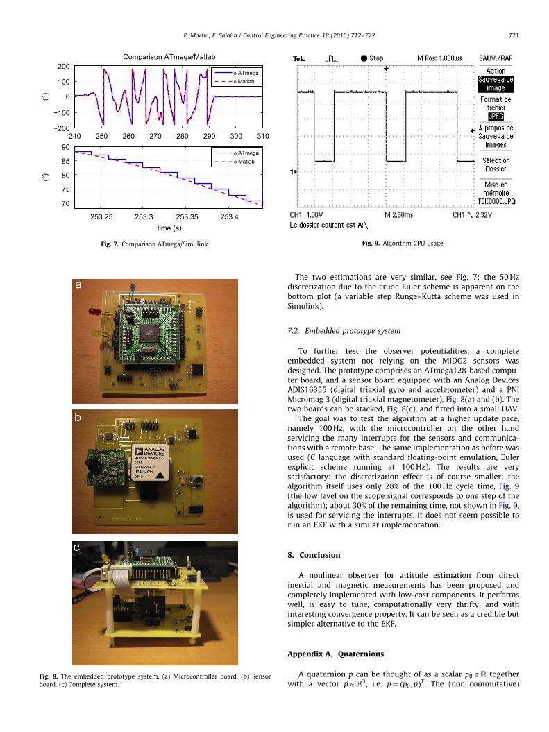

ARTICLE IN PRESS

240 250 260 270 280 290 300 310−200

−100

0

100

200Comparison ATmega/Matlab

(°)

253.25 253.3 253.35 253.4

70

75

80

85

90

(°)

time (s)

φ ATmegaφ Matlab

φ ATmegaφ Matlab

Fig. 7. Comparison ATmega/Simulink.

Fig. 8. The embedded prototype system. (a) Microcontroller board. (b) Sensor

board. (c) Complete system.

Fig. 9. Algorithm CPU usage.

P. Martin, E. Salaun / Control Engineering Practice 18 (2010) 712–722 721

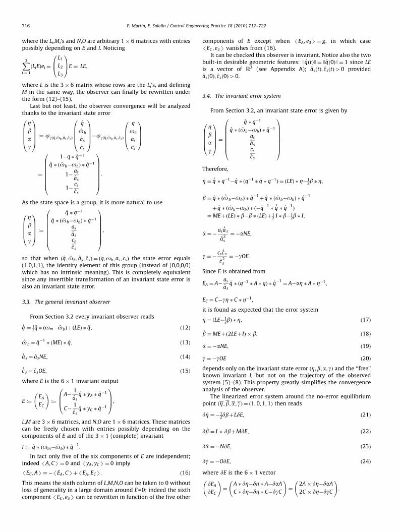
The two estimations are very similar, see Fig. 7; the 50 Hzdiscretization due to the crude Euler scheme is apparent on thebottom plot (a variable step Runge–Kutta scheme was used inSimulink).

7.2. Embedded prototype system

To further test the observer potentialities, a completeembedded system not relying on the MIDG2 sensors wasdesigned. The prototype comprises an ATmega128-based compu-ter board, and a sensor board equipped with an Analog DevicesADIS16355 (digital triaxial gyro and accelerometer) and a PNIMicromag 3 (digital triaxial magnetometer), Fig. 8(a) and (b). Thetwo boards can be stacked, Fig. 8(c), and fitted into a small UAV.

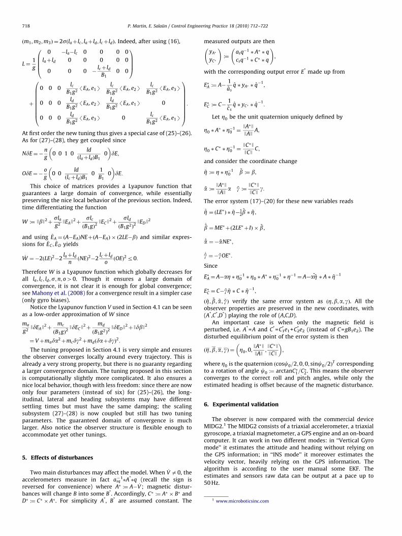
The goal was to test the algorithm at a higher update pace,namely 100 Hz, with the microcontroller on the other handservicing the many interrupts for the sensors and communica-tions with a remote base. The same implementation as before wasused (C language with standard floating-point emulation, Eulerexplicit scheme running at 100 Hz). The results are verysatisfactory: the discretization effect is of course smaller; thealgorithm itself uses only 28% of the 100 Hz cycle time, Fig. 9(the low level on the scope signal corresponds to one step of thealgorithm); about 30% of the remaining time, not shown in Fig. 9,is used for servicing the interrupts. It does not seem possible torun an EKF with a similar implementation.

8. Conclusion

A nonlinear observer for attitude estimation from directinertial and magnetic measurements has been proposed andcompletely implemented with low-cost components. It performswell, is easy to tune, computationally very thrifty, and withinteresting convergence property. It can be seen as a credible butsimpler alternative to the EKF.

Appendix A. Quaternions

A quaternion p can be thought of as a scalar p0AR togetherwith a vector ~pAR3, i.e. p¼ ðp0; ~pÞ

T . The (non commutative)

ARTICLE IN PRESS

P. Martin, E. Salaun / Control Engineering Practice 18 (2010) 712–722722

quaternion product � then reads

p � q :¼p0q0�~p �~q

p0~qþq0~pþ~p �~q

!:

The cross product can be extended to quaternions byp� q :¼ 1

2 ðp � q�q � pÞ ¼~p �~q.Quaternions provide a global parametrization of the orienta-

tion of a rigid body (whereas Euler angles necessarily havesingularities). Indeed, to any quaternion q with unit norm isassociated a rotation matrix RqASOð3Þ by q�1 �~p � q¼ Rq �~p for all~pAR3. Any scalar p0AR can be seen as the quaternion ðp0; ~0Þ

T ,and any vector ~pAR3 as the quaternion ð0; ~pÞT . The quaternions(with non zero norm) form a group with 1 as the identity element,and ðp � qÞ�1

¼ q�1 � p�1.If q depends on time, then _q�1

¼�q�1 � _q � q�1. Finally,consider the differential equation _q ¼ q � uþv � q with u; vAR3;then JqðtÞJ¼ Jqð0ÞJ for all t.

The tangent space at 1 of the unit norm quaternion space canbe identified with R3. Indeed, if q is a unit norm quaternion‘‘close’’ to 1, its differential dq is dq1e1þdq2e2þdq3e3 sinceq2

0þq21þq2

2þq23 ¼ 1 implies q0dq0þq1dq1þq2dq2þq3dq3 ¼ 0,

hence dq0 ¼ 0.

References

Bonnabel, S., Martin, P., & Rouchon, P. (2008). Symmetry-preserving observers.IEEE Transactions on Automatic Control, 53(11), 2514–2526.

Bonnabel, S., Martin, P., & Rouchon, P. (2009). Non-linear symmetry-preservingobservers on lie groups. IEEE Transactions on Automatic Control, 54(7), 1709–1713.

Crassidis, J. L., Markley, F. L., & Cheng, Y. (2007). Survey of nonlinear attitudeestimation methods. Journal of Guidance Control and Dynamics, 30(1), 12–28.

Grewal, M., Weill, L., & Andrews, A. (2007). Global positioning systems, inertialnavigation, and integration (2nd ed.). New York: Wiley.

Kayton, M., & Fried, W. (1997). Avionics navigation systems (2nd ed.). New York:Wiley.

Lefferts, E., Markley, F., & Shuster, M. (1982). Kalman filtering for spacecraftattitude. Journal of Guidance Control and Dynamics, 5(5), 417–429.

Mahony, R., Hamel, T., & Pflimlin, J.-M. (2008). Nonlinear complementary filters onthe special orthogonal group. IEEE Transactions on Automatic Control, 53(5),1203–1218.

Markley, F. (2003). Attitude error representations for kalman filtering. Journal ofGuidance Control and Dynamics, 26(2), 311–317.

Martin, P., & Salaun, E. (2007). Invariant observers for attitude and headingestimation from low-cost inertial and magnetic sensors. In IEEE conference ondecision and control (pp. 1039–1045).

Martin, P., & Salaun, E. (2008a). Design and implementation of a low-cost attitudeand heading nonlinear estimator. In International conference on informatics incontrol, automation and robotics (pp. 53–61).

Martin, P., & Salaun, E. (2008b). A general symmetry-preserving observer forattitude and heading reference systems. In IEEE conference on decision andcontrol (pp. 2294–2301).

Martin, P., & Salaun, E. (2008c). An invariant observer for Earth-velocity-aidedattitude heading reference systems. In IFAC World Congress. Paper identifier10.3182/20080706-5-KR-1001.3577.

Martin, P., & Salaun, E. (2010). The true role of accelerometer feedback inquadrotor control. In IEEE international conference on robotics and automation.Preliminary version /http://hal.archives-ouvertes.fr/hal-00422423/en/S.

Metni, N., Pfimlin, J.-M., Hamel, T., & Sou�eres, P. (2006). Attitude and gyrobias estimation for a flying UAV. Control Engineering Practice, 14,1114–1120.

Pflimlin, J.-M., Binetti, P., Sou �eres, P., Hamel, T., & Trouchet, D. (2010). Modelingand attitude control analysis of a ducted-fan micro aerial vehicle. ControlEngineering Practice, in press, doi: 10.1016/j.conengprac.2009.09.009.

Shuster, M., & Oh, S. (1981). Three-axis attitude determination from vectorobservations. Journal of Guidance Control and Dynamics, 4(1), 70–77.

Stevens, B., & Lewis, F. (2003). Aircraft control and simulation (2nd ed.). New York:Wiley.

Thienel, J., & Sanner, R. (2003). A coupled nonlinear spacecraft attitude controllerand observer with an unknown constant gyro bias and gyro noise. IEEETransactions on Automatic Control, 48(11), 2011–2015.