Design and Implementation of a CVRP simulator by

means of Genetic Algorithms

Iván Ramírez Cortes1, José Alberto Hernández Aguilar

23, Miguel Ángel Ruiz

1, Marco

Antonio Cruz2 and G. Arroyo-Figueroa

3

1 Polytechnic University of the State of Morelos, Boulevard Paseo Cuauhnáhuac 566, Lomas

del Texcal, 62550 Jiutepec, Mor., México 2 Autonomous University of the State of Morelos, Av. Universidad 1001, Chamilpa, 62209

Cuernavaca, Mor., México. 3 National Institute of Electricity and Clean Energies, Reforma 113, Palmira, 62490 Cuernava-

ca, Mor., México

jose_hernandez@uaem.mx

Abstract. We discuss the design and implementation of a CVRP simulator, for

this purpose firstly, we discuss briefly CVRP and its taxonomy, later we discuss

in depth the genetic algorithm (GA), further we present the design and imple-

mentation of a three-tier web-based system to upload a CVRP instance and se-

lect a Metaheuristic for its processing. For probing our simulator, we calculate

the best route(s), processing ten different .vrp instances, with our GA and com-

pare it with the nearest neighbor algorithm (NNA). Preliminary results show

genetic algorithm generates some best routes, but processing time is higher re-

garding nearest neighbor algorithm.

Keywords: CVRP, simulation, genetic algorithm, nearest neighbor algorithm,

client-server technology.

1 Introduction

Research problem

It has been identified that in the state of Morelos, Mexico, small and medium busi-

nesses need a logistics in real time to solve routing problems, which requires the im-

plementation of a plotter of routes to represent real-world instances of the CVRP (Ca-

pacitated Vehicle Routing Problem) that meets following features:

Operate under three tiers client-server architecture

Allows the reading of .vrp files from the client-side, send the request to the server,

select the algorithm or heuristic goal to use (for example nearest neighbor, ants colo-

ny, genetic). Call the corresponding method and display in real time the results of the

progress in the process of optimization of the route. Is required the use of java run-

ning on a web platform for the implementation of the plotter of routes for the CVRP

by intelligent algorithms, since the server will be mounted on open source software.

1.1. Justification

The research group UAEMOR CA124 “Operations research and computer sci-

ence”, participated in the convocation of the PRODEP 2015 for the creation of aca-

demic networks, derived from this convocation was obtained financial support for the

implementation of several projects, within these projects was financed the corre-

sponding plotter for the solution of the CVRP, which for its complete solution in-

cludes not only the estimate of the calculation for routes but its real-time plotting.

At present, the lack of simulators that graph in real time this type of problems is

very wide, and it is even more difficult to find simulators operating via the client-

server architecture.

1.2 Hypothesis

Hi. Using a graphing tool for problems CVRP type, operating under the client-

server architecture, allows determining if genetic algorithms obtained better results

than the nearest neighbor algorithm.

Ho. Using a graphing tool for problems CVRP type, operating under the client-

server architecture, does not allow determining if genetic algorithms do not obtain

better results than the nearest neighbor algorithm.

1.3 Scope and limitations

Scope

We analyze the problem and abstract its requirements in four modules:

Module of reading of .vrp instances

The system will be able to read files of .vrp type previous proper validation.

Module of parameters selection

Type of Technology to use for the server process: sequential, parallel.

Select the type of algorithm to simulate (genetic algorithm).

Module of nodes graphing in real time

Plots the local optimal routes regularly, showing where the user will be able

to select the best-desired route.

Module of Graphical Export

Once calculated the best route, it could be exported in JPG or PNG format, as

well as the summary of information (total distance and processing time).

Methodology for development: Extreme programming

XP is an agile methodology for software development, basically consists in strict

adherence to a set of rules that are focused on the needs of the client in order to

achieve a good quality product in a short time, focused on enhancing relationships as

key to the success of software development. The philosophy of XP is to satisfy the

customer’s needs, integrating it as part of the development team. In all the iterations

of this cycle, both the client and the program learn.

Structure of document

In section one we describe the problem at hands, section two discuss related work,

including VRP theory, its taxonomy and main approaches to solve it, we focus in

genetic algorithm metaheuristics as a method of solution. Later we discuss CVRP

mathematical model. In section three, we present the implementation of the CVRP

simulator based on the client-server technology; we present pseudo code of main

functions and include segments of Matlab code created to implement a genetic algo-

rithm to solve CVRP instances. Finally, we present preliminary results, conclusions,

and future work.

2 Related work

2.1 VRP

The Vehicle Routing Problem (VRP) is used to determine a set of routes for a fleet of

vehicles that are based on one or more deposits or warehouses, to satisfy the demand

of multiple customers geographically dispersed proposed by Hillier and Lieberman

[10]. According [14] importance of VRP is due:

“The transport of goods in urban environments plays a very important role in the

sustainable development of a city, as high levels of movement of goods occur

within cities”.

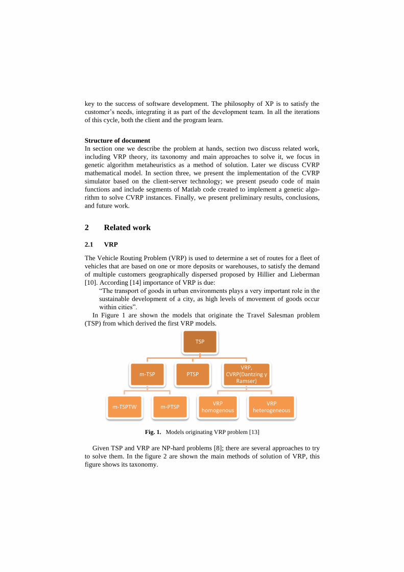
In Figure 1 are shown the models that originate the Travel Salesman problem

(TSP) from which derived the first VRP models.

Fig. 1. Models originating VRP problem [13]

Given TSP and VRP are NP-hard problems [8]; there are several approaches to try

to solve them. In the figure 2 are shown the main methods of solution of VRP, this

figure shows its taxonomy.

TSP

m-TSP

m-TSPTW m-PTSP

PTSP VRP,

CVRP(Dantzing y Ramser)

VRP homogenous

VRP heterogeneous

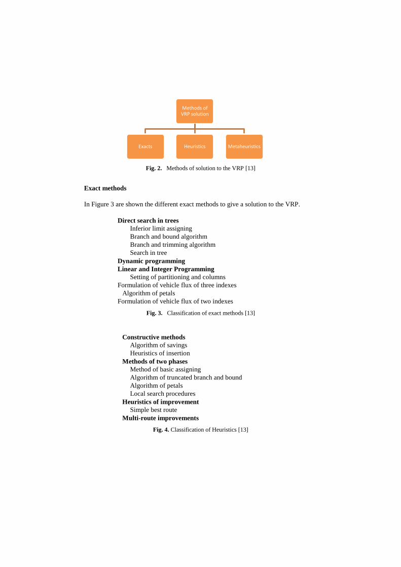
Fig. 2. Methods of solution to the VRP [13]

Exact methods

In Figure 3 are shown the different exact methods to give a solution to the VRP.

Direct search in trees

Inferior limit assigning

Branch and bound algorithm

Branch and trimming algorithm

Search in tree

Dynamic programming

Linear and Integer Programming

Setting of partitioning and columns

Formulation of vehicle flux of three indexes

Algorithm of petals

Formulation of vehicle flux of two indexes

Fig. 3. Classification of exact methods [13]

Constructive methods

Algorithm of savings

Heuristics of insertion

Methods of two phases

Method of basic assigning

Algorithm of truncated branch and bound

Algorithm of petals

Local search procedures

Heuristics of improvement

Simple best route

Multi-route improvements

Fig. 4. Classification of Heuristics [13]

Methods of VRP solution

Exacts Heuristics Metaheuristics

Heuristics

The heuristics are procedures that provide acceptable quality solutions limited

through an exploration of the search space [4].These methods are based on routes that

contain a single node to find the best pair (node, route) that represents the best inter-

section [11]. Figure 4 shows the classification of the heuristics in constructive meth-

ods, methods of two phases and heuristics of improvement.

Metaheuristics

Most of these methods of solution were developed in the 1990s; one of its features is

that procedures of search try to find acceptable solutions [5]. In figure 5, are shown

these methods of solution that consist of Simulated Annealing, Taboo Search, Neural

Networks, Genetic algorithms, ant colony algorithms and search in neighborhoods.

Genetic algorithms

Artificial neuronal networks

Simulated Annealing

Deterministic annealing

Ant Colony algorithm

Taboo Search

Adaptive memory procedure

Search in neighborhood “VNS”

Fig. 5. Classification of Metaheuristics [13]

2.2 Genetic algorithm

Genetic Algorithms (AGs) are adaptive methods that can be used to solve problems

arising from the search and optimization [13]. They are based in the genetic process in

living organisms [2, 7]. It is based on the principles of the laws of the natural life

proposed by Darwin. A genetic algorithm according to [9] basically consists of 1) An

initial population, which can be generated in a random way, 2) Calculation of the

fitness function, 3) Selection based on the fitness of the population, 4) Generate a new

population through cross and mutation, 5) Generate a cycle of the above until the

function of unemployment is true. And 6) get the best population of individuals.

Pseudo code of genetic algorithm [9]

BEGIN A /*Simple Genetic Algorithm */

Generate an initial population.

Compute the fitness function of each individual.

WHILE NOT Finished DO

BEGIN to /*produce new generation*/

FOR POPULATION SIZE / 2 DO

BEGIN /*Reproductive cycle*/

Select two individuals of the previous gener-

ation, for the crossing (probability of se-

lection proportional the evaluation function

of the individual).

Cross with a certain probability the two in-

dividuals obtaining two descendants.

Mutate The two descendants with a certain

probability.

Compute the evaluation function of the

two mutated descendants.

Insert the two mutated descendants in the new

generation.

END

IF the population has converged, THEN

Completed = True

END

END

Mathematical model for the CVRP

The CVRP has as an objective function which purpose is to minimize the costs of the

vehicles in the trajectories. Table 1 displays a list of the indexes and variables that

occupies the mathematical model of the CVRP.

Table 1. Indexes and variables of CVRP model

Nomenclature Description Nomenclature Description

I The node of the

departure of the

vehicle.

Cij Cost of transport

of the node i to

node j

J The node of the

departure of the

vehicle.

Dj Demand in the

node j

d Vehicle to use

(1,2,3,…k)

U Resource ca-

pacity k

xijk Customer Demand N Number of cli-

ents

Yij If it is equal to 1,

the vehicle k is

assigned to the arc

from node i to

node j. It is equal

to 0 otherwise

The mathematical model of CVRP routing, according to [1, 12], is:

𝑀𝑖𝑛𝑖𝑚𝑖𝑧𝑒 ∑ 𝑐𝑖𝑗 ∗ 𝑦𝑖𝑗(𝑖,𝑗)∈𝐴 (1)

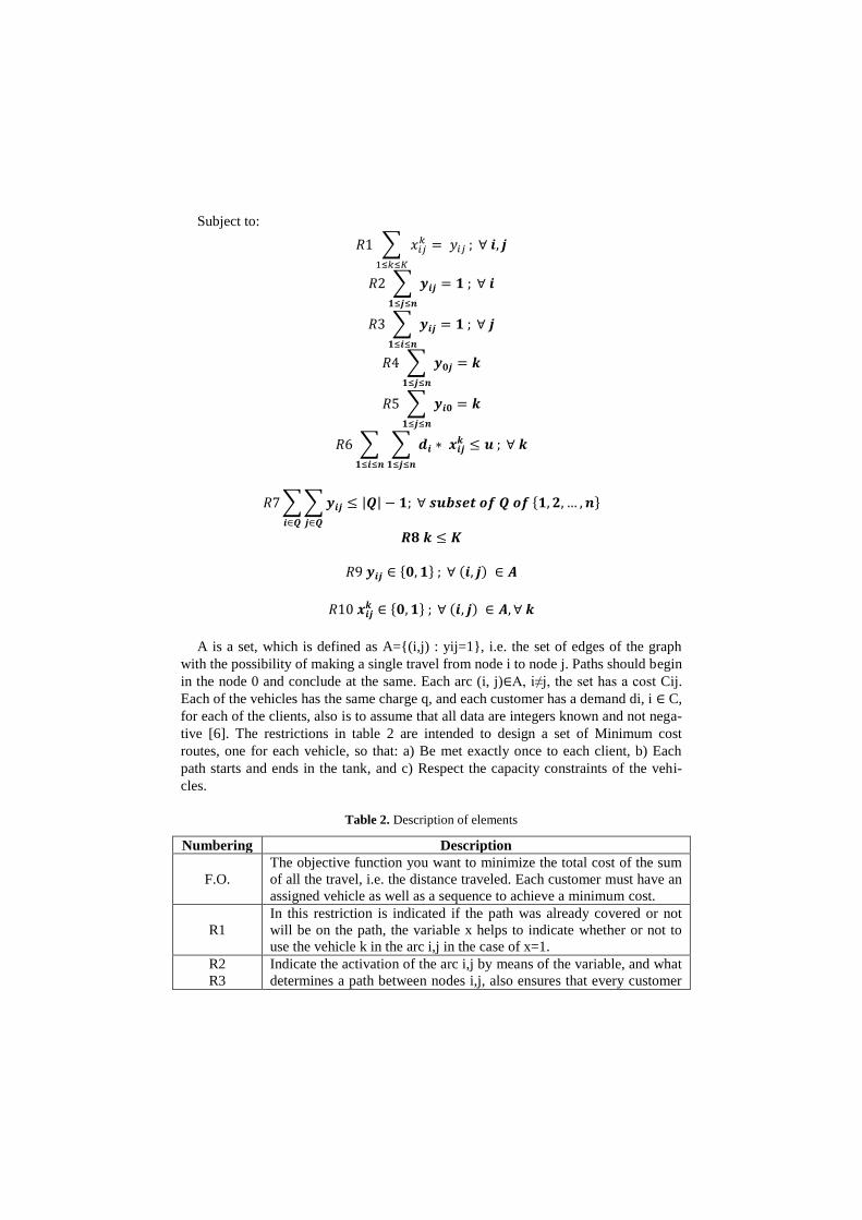
Subject to:

𝑅1 ∑ 𝑥𝑖𝑗𝑘 = 𝑦𝑖𝑗

1≤𝑘≤𝐾

; ∀ 𝒊, 𝒋

𝑅2 ∑ 𝒚𝒊𝒋 = 𝟏 ; ∀ 𝒊

𝟏≤𝒋≤𝒏

𝑅3 ∑ 𝒚𝒊𝒋

𝟏≤𝒊≤𝒏

= 𝟏 ; ∀ 𝒋

𝑅4 ∑ 𝒚𝟎𝒋

𝟏≤𝒋≤𝒏

= 𝒌

𝑅5 ∑ 𝒚𝒊𝟎 = 𝒌

𝟏≤𝒋≤𝒏

𝑅6 ∑ ∑ 𝒅𝒊

𝟏≤𝒋≤𝒏𝟏≤𝒊≤𝒏

∗ 𝒙𝒊𝒋𝒌 ≤ 𝒖 ; ∀ 𝒌

𝑅7 ∑ ∑ 𝒚𝒊𝒋 ≤ |𝑸|

𝒋∈𝑸𝒊∈𝑸

− 𝟏; ∀ 𝒔𝒖𝒃𝒔𝒆𝒕 𝒐𝒇 𝑸 𝒐𝒇 {𝟏, 𝟐, … , 𝒏}

𝑹𝟖 𝒌 ≤ 𝑲

𝑅9 𝒚𝒊𝒋 ∈ {𝟎, 𝟏} ; ∀ (𝒊, 𝒋) ∈ 𝑨

𝑅10 𝒙𝒊𝒋𝒌 ∈ {𝟎, 𝟏} ; ∀ (𝒊, 𝒋) ∈ 𝑨, ∀ 𝒌

A is a set, which is defined as A={(i,j) : yij=1}, i.e. the set of edges of the graph

with the possibility of making a single travel from node i to node j. Paths should begin

in the node 0 and conclude at the same. Each arc (i, j)∈A, i≠j, the set has a cost Cij.

Each of the vehicles has the same charge q, and each customer has a demand di, i ∈ C,

for each of the clients, also is to assume that all data are integers known and not nega-

tive [6]. The restrictions in table 2 are intended to design a set of Minimum cost

routes, one for each vehicle, so that: a) Be met exactly once to each client, b) Each

path starts and ends in the tank, and c) Respect the capacity constraints of the vehi-

cles.

Table 2. Description of elements

Numbering Description

F.O.

The objective function you want to minimize the total cost of the sum

of all the travel, i.e. the distance traveled. Each customer must have an

assigned vehicle as well as a sequence to achieve a minimum cost.

R1

In this restriction is indicated if the path was already covered or not

will be on the path, the variable x helps to indicate whether or not to

use the vehicle k in the arc i,j in the case of x=1.

R2

R3

Indicate the activation of the arc i,j by means of the variable, and what

determines a path between nodes i,j, also ensures that every customer

is an intermediate node of any route. That is to say, that ensures that

each client is visited once by a vehicle.

R4

R5

R6

Indicate that k is the number of vehicles used in the solution and that

all those who depart from the deposit must be returned to the same.

R7 Notes that each vehicle does not exceed its capacity.

R8 Monitors that the solution does not contain cycles using 1.2 nodes,

…n. Otherwise, the arches to contain any cycle passing through a set

of nodes Q and the solution would violate the constraint because the

left side of the restriction would be at least |Q|.

R9 Limits the maximum number of vehicles to use up to a maximum

amount.

R10 Indicate that the variables x, y are binary

3 Implementation of CRVP simulator

The following are the modules implemented within the simulator and shown in Figure

6.

Fig. 6. Functional description of CVRP Simulator

File validation

For a correct operation of programs is mandatory to validate that the .vrp file has a

correct structure. This function validates a .vrp extension, and description of file con-

tent: name, comment, type, dimension, edge type, weight type, and capacity.

Module of File reading

This module is intended to validate the reading of the files of type .vrp taking into

account: a) At the time of actually read a file; b) the extension is correct (.vrp); c)

Correct structure, d) titles are spelled correctly.

Reading of file

As a first step, the simulator reads a file .vrp. To be able to read the file is imple-

mented the next pseudo code using java.

Setting of instances for Java and Matlab

This function creates instances from Java to be able to be used in Matlab. Through the

use of functions to read from and write to files, the file includes an identifier, coordi-

nates x & y and the demand, the function creates a new .m extension file.

Fig. 7. Example of m file created in Java and compatible with Matlab

Server Side Module

In figure 6 is shown in the diagram corresponding to the server side, in which Matlab

receives the .m file generated in Java, read the coordinates, and uses a genetic algo-

rithm to perform calculations of routes and produce its graph interacting with Matlab.

Implementation of the genetic algorithm

In order to obtain the optimal routes, we implemented a genetic algorithm in Matlab,

next are displayed the most important functions.

Selection by tournament

For the implementation of the selection was used tournament, Matlab code is shown

next:

Selection by tournament Matlab code

T = round (random (2*N, S) * (5) +1;

% Tournament

[d, idx] = max (F(t),[],2); % index to determine winners

W = T(sub2ind (size(t), (1:2*N)’, idx)); %winners

Crossover

We used one point crossover. Matlab code is shown below:

One point crossover (Matlab code)

Pop2 = Pop (W(1:2: FIN),1:)% First winners variable of

Pop2

P2A = Pop (W(2:2:FIN),:)% Second winners variable of Pop2

Lidx = sub2ind (size (Pop), round (random(N,1)*(5)+1)

Next Matlab code shows the selection process to perform the crossover

Selection process to perform crossover (Matlab code)

% Selection of one point

vLidx= P2A(Lidx)*(1,G) % Point of two winners

[r,c] = find (Pop2 == vLidx) %winners 1

[d, Ord] = sort( r ) %Sort linear index

r = r (Ord); c = c (ord) % Reorder index

Lidx2 = sub2ind(size(Pop), r, c) % Convert to one index

Pop2(Lidx2) = Pop2(Lidx) % Half of crossover 1

Mutation

Finally there is the stage of mutation which is shown next:

Mutation (Matlab code)

Idx = rand (N,1) < Muta % Selection of individuals to

permute

Loc1 = sub2ind(size(Pop2), 1: N, round(random(1,N) *(5)

+1)) % Interchange of index 2

Loc 2 = sub2ind(size(Pop2), 1: N, round(random(1,N) *(5)

+1)) % Interchange of index 2

Loc2 (idx == 0) = Loc1 (idx == 0) % Probability of muta-

tion

[Pop2 (Loc1), Pop2(Loc2) ] = deal (Pop2(Loc2),

Pop2(Loc1)) % Mutation

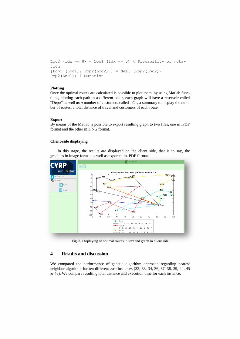
Plotting

Once the optimal routes are calculated is possible to plot them, by using Matlab func-

tions, plotting each path to a different color, each graph will have a reservoir called

“Depo” as well as n number of customers called “C”, a summary to display the num-

ber of routes, a total distance of travel and customers of each route.

Export

By means of the Matlab is possible to export resulting graph to two files, one in .PDF

format and the other in .PNG format.

Client-side displaying

In this stage, the results are displayed on the client side, that is to say, the

graphics in image format as well as exported in .PDF format.

Fig. 8. Displaying of optimal routes in text and graph in client side

4 Results and discussion

We compared the performance of genetic algorithm approach regarding nearest

neighbor algorithm for ten different .vrp instances (32, 33, 34, 36, 37, 38, 39, 44, 45

& 46). We compare resulting total distance and execution time for each instance.

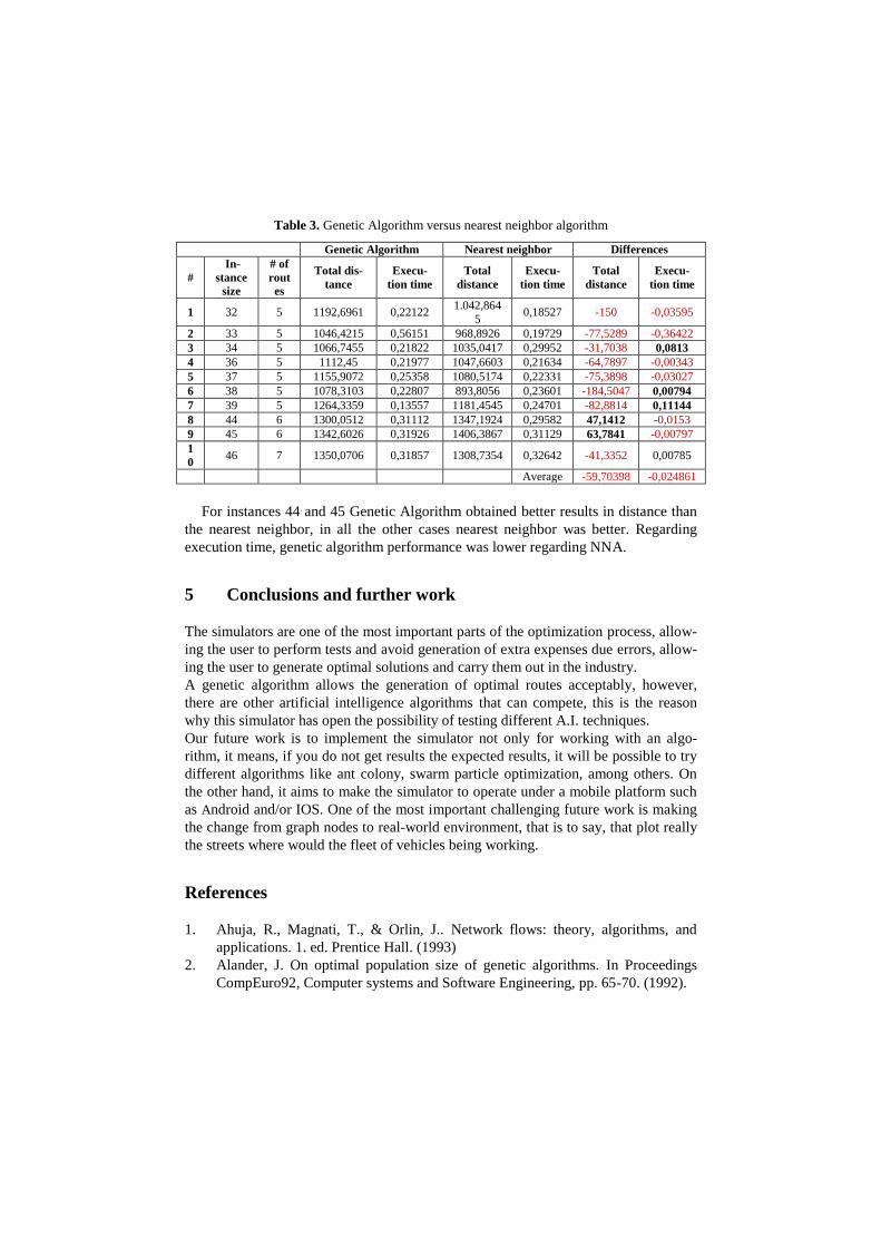
Table 3. Genetic Algorithm versus nearest neighbor algorithm

Genetic Algorithm Nearest neighbor Differences

# In-

stance

size

# of

rout

es

Total dis-

tance Execu-

tion time Total

distance Execu-

tion time Total

distance Execu-

tion time

1 32 5 1192,6961 0,22122 1.042,864

5 0,18527 -150 -0,03595

2 33 5 1046,4215 0,56151 968,8926 0,19729 -77,5289 -0,36422

3 34 5 1066,7455 0,21822 1035,0417 0,29952 -31,7038 0,0813

4 36 5 1112,45 0,21977 1047,6603 0,21634 -64,7897 -0,00343

5 37 5 1155,9072 0,25358 1080,5174 0,22331 -75,3898 -0,03027

6 38 5 1078,3103 0,22807 893,8056 0,23601 -184,5047 0,00794

7 39 5 1264,3359 0,13557 1181,4545 0,24701 -82,8814 0,11144

8 44 6 1300,0512 0,31112 1347,1924 0,29582 47,1412 -0,0153

9 45 6 1342,6026 0,31926 1406,3867 0,31129 63,7841 -0,00797

1

0 46 7 1350,0706 0,31857 1308,7354 0,32642 -41,3352 0,00785

Average -59,70398 -0,024861

For instances 44 and 45 Genetic Algorithm obtained better results in distance than

the nearest neighbor, in all the other cases nearest neighbor was better. Regarding

execution time, genetic algorithm performance was lower regarding NNA.

5 Conclusions and further work

The simulators are one of the most important parts of the optimization process, allow-

ing the user to perform tests and avoid generation of extra expenses due errors, allow-

ing the user to generate optimal solutions and carry them out in the industry.

A genetic algorithm allows the generation of optimal routes acceptably, however,

there are other artificial intelligence algorithms that can compete, this is the reason

why this simulator has open the possibility of testing different A.I. techniques.

Our future work is to implement the simulator not only for working with an algo-

rithm, it means, if you do not get results the expected results, it will be possible to try

different algorithms like ant colony, swarm particle optimization, among others. On

the other hand, it aims to make the simulator to operate under a mobile platform such

as Android and/or IOS. One of the most important challenging future work is making

the change from graph nodes to real-world environment, that is to say, that plot really

the streets where would the fleet of vehicles being working.

References

1. Ahuja, R., Magnati, T., & Orlin, J.. Network flows: theory, algorithms, and

applications. 1. ed. Prentice Hall. (1993)

2. Alander, J. On optimal population size of genetic algorithms. In Proceedings

CompEuro92, Computer systems and Software Engineering, pp. 65-70. (1992).

3. Bremermann, H. Optimization through evolution and recombination. In: Self-

Organizing systems. Washington, D.C.: M.C. Yovitts et al., Spartan Books.

(1962).

4. Butrón, A. A. Asignación de rutas de vehículos para un sistema de recolección

de residuos sólidos en la acera. Revista de Ingeniería, 13(5), pp. 5-11. (2001).

5. Contardo, C. Formulación y solución de un problema de ruteo de vehículos con

demanda variable en tiempo real, trasbordos y ventanas de tiempo. Santiago de

Chile, Chile: Universidad de Chile. (2005).

6. Dorigo, M., & Gambardella, L. Biosystems. ElSEVIER, 43(2), pp. 73-81.

(1997).

7. Fraser, A. S. Simulation of genetic systems by automatic digital computers. I.

Introduction. Aust. J. Biol. Sci., 10, pp. 484-491. (1957).

8. Garey, M., & Johnson, D. Computers and intractability. A Guide to the Theory

of NP-Completeness. NY, USA: W. H. Freeman & Co. (1990).

9. Goldberg, D. Genetic algorithms in Search Optimization and Machine Learning.

Boston, MA, USA, Addison-Wesley, (1989).

10. Hillier, F., & Lieberman, G. J. Introducción a la Investigación de Operaciones

8th

ed. McGraw-Hill/Interamericana Editores, Ed., México. (2006).

11. Laporte, G., Gendreau, M., & Hertz, A. An approximation algorithm for the

traveling salesman problem with time windows. Operations Research, 45(4), pp.

639-641. (1998).

12. Olivera, A. Heurísticas para problemas de ruteo de vehículos. Uruguay. (2004).

13. Rocha, L., González, C., & Orjuela, J. Una revisión al estado del arte del

problema de ruteo de. Ingeniería: Evolución histórica y métodos de solución,

Ingeniería 16(2), pp. 35-55. (2011).

14. Thompson, R. G., & Van Duin, J. H. Vehicle routing and scheduling. En E.

Taniguchi, & T. R.G., Innovations in freight transportation. pp. 47-63.

Southampton: WIT Press. (2003).