DESIGN AND EXPERIMENTATION OF A TUNABLY

COMPLIANT ROBOTIC FINGER USING

LOW MELTING POINT METALS

by

HEON JOO

A thesis submitted in partial fulfillment ofthe requirements for the degree of

MASTER OF SCIENCE IN MECHANICAL ENGINEERING

WASHINGTON STATE UNIVERSITYDepartment of Mechanical and Materials Engineering

JULY 2017

c© Copyright by HEON JOO, 2017All Rights Reserved

c© Copyright by HEON JOO, 2017All Rights Reserved

To the Faculty of Washington State University:

The members of the Committee appointed to examine the thesis of HEON JOO

find it satisfactory and recommend that it be accepted.

John Swensen, Ph.D., Chair

Arda Gozen, Ph.D.

Matthew Taylor, Ph.D.

ii

ACKNOWLEDGMENTS

I would like to thank my advisor, Dr.Swensen who has taught and guided so

far for this thesis completion and also thank Dr.Taylor for joining me in his project.

During the last two years, my wife sincerely supported me with a lot of courage and

hope and my son was another delight that made me endure here to the end. I would

like to express my deepest gratitude to all of the families in Korea, especially my

grandmother. She is the most appreciated and precious person in my life that made

me today. Also, I would like to appreciate many Koreans we have known in Pullman.

Lastly, I would like to give my infinite glory and gratitude to God who gave me and

my family the strength, courage, and wisdom to overcome any difficulties.

iii

DESIGN AND EXPERIMENTATION OF A TUNABLY

COMPLIANT ROBOTIC FINGER USING

LOW MELTING POINT METALS

Abstract

by Heon Joo, M.S.Washington State University

July 2017

Chair: John Swensen

In this thesis, it is explaining that the fabrication and testing of a tunably-

compliant tendon-driven finger implemented through the geometric design of a skele-

ton made of the low-melting point Field’s metal encased in a silicone rubber. The

initial prototype consists of a skeleton comprised of two rods of the metal, with heat-

ing elements in thermal contact with the metal at various points along its length,

embedded in an elastomer. The inputs to the systems are both the force exerted on

the tendon to bend the finger and the heat introduced to liquefy the metal locally

or globally along the length of the finger. Selective localized heating allows multiple

joints to be created along the length of the finger.

iv

Fabrication was accomplished via a multiple step process of elastomer casting

and liquid metal casting. Heating elements such as power resistors or Ni-Cr wire with

electrical connections were added as an intermediate step before the final elastomer

casting. The addition of a tradition tendon actuation was inserted after all casting

steps had been completed. While preliminary, this combination of selective heating

and engineered geometry of the low-melting point skeletal structure will allow for

further investigation into the skeletal geometry and its effects on local and global

changes in device stiffness.

v

TABLE OF CONTENTS

ACKNOWLEDGMENTS . . . . . . . . . . . . . . . . . . . . . . . . . . . . . . . . . . . . . . . . . . . . . . . . . . iii

ABSTRACT . . . . . . . . . . . . . . . . . . . . . . . . . . . . . . . . . . . . . . . . . . . . . . . . . . . . . . . . . . . . . . . iv

LIST OF TABLES . . . . . . . . . . . . . . . . . . . . . . . . . . . . . . . . . . . . . . . . . . . . . . . . . . . . . . . . . viii

LIST OF FIGURES . . . . . . . . . . . . . . . . . . . . . . . . . . . . . . . . . . . . . . . . . . . . . . . . . . . . . . . . ix

DEDICATION . . . . . . . . . . . . . . . . . . . . . . . . . . . . . . . . . . . . . . . . . . . . . . . . . . . . . . . . . . . . . xi

1. Introduction . . . . . . . . . . . . . . . . . . . . . . . . . . . . . . . . . . . . . . . . . . . . . . . . . . . . . . . . . . . 1

2. Related Work . . . . . . . . . . . . . . . . . . . . . . . . . . . . . . . . . . . . . . . . . . . . . . . . . . . . . . . . . . 5

3. Design and Fabrication . . . . . . . . . . . . . . . . . . . . . . . . . . . . . . . . . . . . . . . . . . . . . . . . . 10

3.1 Molds Design . . . . . . . . . . . . . . . . . . . . . . . . . . . . . . . . . . . . . . . . . . . . . . . . . . . . . . 11

3.2 Layer Fabrication . . . . . . . . . . . . . . . . . . . . . . . . . . . . . . . . . . . . . . . . . . . . . . . . . . 15

3.3 Finger Manufacturing Process . . . . . . . . . . . . . . . . . . . . . . . . . . . . . . . . . . . . . . 20

4. Experiments . . . . . . . . . . . . . . . . . . . . . . . . . . . . . . . . . . . . . . . . . . . . . . . . . . . . . . . . . . . 26

4.1 Rate of Change of Temperature from 24 ◦C to 62 ◦C . . . . . . . . . . . . . . . . 28

4.2 Fluctuation of Temperature between 50 ◦C and 70 ◦C . . . . . . . . . . . . . . . 30

4.3 The Temperature of Liquefying and Solidifying the Metal . . . . . . . . . . . 32

4.4 Device Actuation and Kinematics . . . . . . . . . . . . . . . . . . . . . . . . . . . . . . . . . . 35

5. Thermal Analysis and Simulation . . . . . . . . . . . . . . . . . . . . . . . . . . . . . . . . . . . . . . . 37

5.1 Thermal Analysis of the Steady State Behavior . . . . . . . . . . . . . . . . . . . . . 40

5.2 Thermal Analysis of Transient Behavior . . . . . . . . . . . . . . . . . . . . . . . . . . . . 46

5.3 Thermal Simulation Using Solidworks FEA . . . . . . . . . . . . . . . . . . . . . . . . . 50

vi

6. Additional Geometric Complexity of the Metal Skeleton . . . . . . . . . . . . . . . . . 61

7. Results and Discussion . . . . . . . . . . . . . . . . . . . . . . . . . . . . . . . . . . . . . . . . . . . . . . . . . 65

8. Conclusion . . . . . . . . . . . . . . . . . . . . . . . . . . . . . . . . . . . . . . . . . . . . . . . . . . . . . . . . . . . . . 70

vii

LIST OF TABLES

Table Page

3.1 Comparison between two silicone compounds . . . . . . . . . . . . . . . . . . . . . . . 16

5.1 Each material’s properties . . . . . . . . . . . . . . . . . . . . . . . . . . . . . . . . . . . . . . . . . 40

viii

LIST OF FIGURES

Figure Page

3.1 Two different kinds of fingers . . . . . . . . . . . . . . . . . . . . . . . . . . . . . . . . . . . . . . 10

3.2 The silicone compound mold . . . . . . . . . . . . . . . . . . . . . . . . . . . . . . . . . . . . . . . 11

3.3 Ni-Cr wire casting mold. . . . . . . . . . . . . . . . . . . . . . . . . . . . . . . . . . . . . . . . . . . . 12

3.4 Field’s metal casting mold . . . . . . . . . . . . . . . . . . . . . . . . . . . . . . . . . . . . . . . . . 13

3.5 Surface mold for tendon driven . . . . . . . . . . . . . . . . . . . . . . . . . . . . . . . . . . . . . 14

3.6 Ni-Cr wiring layer casting process . . . . . . . . . . . . . . . . . . . . . . . . . . . . . . . . . . 17

3.7 Field’s metal rods casting process . . . . . . . . . . . . . . . . . . . . . . . . . . . . . . . . . . 18

3.8 Top surface layer casting process . . . . . . . . . . . . . . . . . . . . . . . . . . . . . . . . . . . 19

3.9 Layer by layer process of sample A and B . . . . . . . . . . . . . . . . . . . . . . . . . . 20

3.10 Fabrication process of sample A . . . . . . . . . . . . . . . . . . . . . . . . . . . . . . . . . . . . 22

3.11 Fabrication process of sample B . . . . . . . . . . . . . . . . . . . . . . . . . . . . . . . . . . . . 24

3.12 Completion of sample A and B . . . . . . . . . . . . . . . . . . . . . . . . . . . . . . . . . . . . . 25

4.1 Experiment set-up . . . . . . . . . . . . . . . . . . . . . . . . . . . . . . . . . . . . . . . . . . . . . . . . . 27

4.2 Finger device bending observation . . . . . . . . . . . . . . . . . . . . . . . . . . . . . . . . . . 36

5.1 One-dimensional conduction heat flow . . . . . . . . . . . . . . . . . . . . . . . . . . . . . . 38

5.2 Section view of sample A . . . . . . . . . . . . . . . . . . . . . . . . . . . . . . . . . . . . . . . . . . 41

5.3 The thermal resistances circuit for the heat transfer . . . . . . . . . . . . . . . . 42

5.4 Temperature dynamics of a heated object . . . . . . . . . . . . . . . . . . . . . . . . . . 46

5.5 Model design of sample A and B . . . . . . . . . . . . . . . . . . . . . . . . . . . . . . . . . . . 50

ix

6.1 More complex skeletal structure like lattice . . . . . . . . . . . . . . . . . . . . . . . . . 61

6.2 Bending moment according to the local heating lines . . . . . . . . . . . . . . . 62

6.3 Fabrication process of lattice structure sample . . . . . . . . . . . . . . . . . . . . . . 63

6.4 Sample of more complex structure and its bending moment . . . . . . . . . 64

x

Dedication

This thesis is dedicated to my grandmother, Youngja Choi who has given huge

endeavor and all sacrifices for me throughout her lifetime and to my aunt,

Youngsook Joo who loved and cared me greatly. Also, I dedicate this thesis to the

companion of my life, Hyojeong Byeon, and my lovely son, Sihwan Joo, and all of

the families in my home country. I am very grateful to the God about this work.

xi

CHAPTER 1. INTRODUCTION

In 2011, the U.S. National Science Foundation announced an ongoing effort

entitled the National Robotics Initiative, whose primary objective is to “develop

robots that work with or beside people to extend or augment human capabilities,

taking advantage of the different strengths of humans and robots.” This emphasis

on humans and robots working the same environments – a component of what has

come to be known as co-robotics – has increased research interest in the area of soft

robotics. The early research in this area of soft robots has tended to be made wholly of

soft elastomers and actuation using either tendons or compressed air. One of the key

limitations of the current state of the art in soft robotics is that, while able to safely

interact with human collaborators, their inherent high degree of compliance limits the

degree to which they can interact with their environment. They have limited ability

to exert forces and conduct manipulations on their surrounding environment because

of their inherent high degree of compliance.

Thus, a principal aim of the proposed work is to create a new type of compliant

robotics, where the robotic materials and structure can switch between acting as a

traditional rigid robotic design and the new class of soft robotic designs. Though only

discussed on a macroscopic scale in this thesis, the eventual goal is compliant devices

1

that change their stiffness in a broad range of spatiotemporal scales. In general,

it is somewhat complicated and difficult to design and fabricate a robotic finger

with this kind of tunable stiffness using traditional methods. Mechanical structures

comprised of components such as motors, linkages, and gears can be used to create

a structure capable of retaining specific shapes, but their use increases the system’s

complexity, and they are generally not capable of producing complex and continuous

deformations [1]. However, by using smart materials, such as the low melting point

Field’s metal, embedded in elastomers and other soft-robotic materials, it becomes

easier to fabricate soft robotic components that exhibit this tunable behavior. Field’s

metal or Field’s alloy is a fusible alloy that becomes liquid at approximately 62 ◦C

(144 ◦F) [2]. It is a eutectic alloy that the solid and liquid temperatures are the same

and composed of bismuth, indium, and tin with the following percentages by weight:

32.5% Bi, 51% In, 16.5% Sn [2].

A standard approach to soft robotics has been the construction of components

made entirely of silicone with fluid-filled cavities for sensing and actuation. This

silicone body approach has helped to shape the idea of a truly “soft” robot since

most of the body is formed out of a soft, elastomeric material with an extremely low

stiffness [3, 4]. Many of the silicone elastomers used in soft robotics are capable of

sustaining its strain anywhere from 100-500% rate of high deformation [3, 4]. This

soft elastomer silicone is used to wrap up the Field’s metal shaped like a long rod and

2

the Ni-Cr wires comprise layers above and below the metal skeleton. When electric

current flows through the Ni-Cr wire, and it becomes hot, the temperature will go up

to the point of melting the Field’s metal inside the silicone. When the metal inside

melts, the silicone can be bent with the metal rods like bending a finger. Elastomers

with electrically controlled stiffness have the potential to revolutionize robotics and

assistive wearable technologies by allowing actuators to independently and reversibly

change both their shape and elastic rigidity [5]. Many variable stiffness actuators

require complicated design a machining to achieve a change of stiffness in even a single

degree of freedom [6, 7, 8]. However, the approach using a low melting temperature

metal alloy provides new ideas, for instance, the latch-able microvalve is able to stay

closed or open from the different state of the metal alloy by the temperature. The

approach with the low melting point metal alloy also can make the elastic rigidity of

soft elastomer tunable by the electrically controlled heating element [2, 5].

In this thesis, we deal with an initial device design with two rods of low melting

point Field’s metal alloy as a skeleton, Ni-Cr wire, and power resistors as a heater and

thermocouples to track the internal heating and cooling of the compliant device. All

materials are embedded in a silicone rubber and the whole device can be actuated by

the tendon routed on the top surface when the state of metal rods are changed by the

temperature. These could be a building block for many soft robotic structures, but

we pose the problem as the core of a tunably-compliant robotic finger. The primary

3

contribution is an investigation of the ability to bias the temperature of the compliant

device to near the melting point of the metal and then observing the rate at which

the mechanism can switch between its stiff and compliant regimes.

4

CHAPTER 2. RELATED WORK

Animals exploit soft structures to move effectively in complex natural environ-

ments. These capabilities have inspired robotic engineers to incorporate soft tech-

nologies into their designs [9, 10]. For example, elephant’s nose is analogous to their

hand. They can freely move their long nose’s muscles to move to the desired position,

and the shape of the tip is similar to the hand that can naturally grab things. The

nose of the elephant evokes the desire of robot researchers to create robotic arms

and hands that are perfectly similar. As early work in the field of biomimetic long

dexterous robots, Walker and Hannan developed a novel hyper-redundant robot ma-

nipulator which featured a backbone of 32 degrees of freedom, with 8 independently

driven tendons to achieve motion and shape adaptation capabilities similar to an

elephant [11, 12]. Actuation is provided via a series of tendons routed through the

structure. In function, the manipulator has capabilities similar to that of the trunk of

an elephant, with the ability to bend into numerous shapes and conform easily to the

environment [11, 12]. For the hardware design, they designed each segment which can

serve as a method for routing the cables. With the series combination of the segments

can give the manipulator its defining shapes. The overall motion of the manipulator

is controlled by a tendon (cable) servo system [11]. The idea inspired by the motion

5

of the elephant nose was analogously able to be feasible by using a noble design of

continuous circular segments that can be connected to the tendon and the motor that

manipulates each tendon for the nose’s locomotion. Other biomimetic approaches

to soft robotics have used squid, starfish, worms, and other cephalopods as inspira-

tion [13, 14, 15]. “Multi-gait Soft Robot” was composed exclusively of soft materials

like elastomeric polymers. Soft lithography was used to fabricate a pneumatically

actuated robot capable of sophisticated locomotion, for example, fluid movement of

limbs and multiple gaits. This robot is quadrupedal and it uses no sensors but only

five actuators with a simple pneumatic valving system that operates at low pressures

below 10psi. A combination of crawling and undulation gaits allowed this robot to

navigate a difficult obstacle [13].

In addition to the robots that imitate the movement of soft animals, there have

been many studies to make the motions of human beings surrounded by soft skin and

muscles to the robotic devices. In particular, the materials such as silicone elastomer

have been mainly used, which can soften and adjust the stiffness in various ways,

without using the existing conventional hard materials, to make this kind of grippers

which can imitate the human hand and pick up something. “Monolithic Fabrication

of Sensors and Actuators in a Soft Robotic Gripper” is a fluidically functionalized

soft-bodied robot that integrates both sensing and actuation [4]. There are two

specific designed molds to cast the robot. The primary one, initially filled with

6

the liquid elastomer, with an inset showing the embossed channels that create the

sensor channels. Another one is the channel mold that is placed in the primary

mold to create the pneumatic channels in the robot [4]. Briefly speaking about the

fabrication, the bottom half of the mold is printed and filled with liquid elastomer.

The channel mold is embedded inside the liquid elastomer to create the pneumatic

channels. When the elastomer has cured, the mold can be removed from around

it. To finish the sensors, the channels are filled with liquid metal (eutectic Indium

Gallium alloy: eGaIn) and sealed with the liquid elastomer. Finally, the pneumatic

channels are sealed by bonding the body to a thin layer of “Silgard 184” and they

attached it to a compressed air source with a flow valve control system that limited

the gauge pressure to activate the robot [4].

The field of soft robotics has been an ideal platform for the applications of smart

materials actuators and multi-functional materials that incorporate both sensing and

actuation [4]. Much of this research takes inspiration from nature in attempts to imi-

tate the movement of soft animals. In particular, materials such as silicone elastomers

have been used extensively, either as a complete soft robotic device or as an outer

skin on conventional hard materials. A primary method of actuation in soft robotics

has been pneumatic chambers and channels [10, 14, 15, 16, 17]. However, alternative

approaches have employed combinations of multiple smart materials, such as shape

memory alloys, shape memory polymers, or low-melting point metals [5, 18]. The

7

prior state of the art in tunable compliance was traditional variable stiffness actua-

tors with tunable series elastic components. These variable stiffness actuators often

require complicated design, machining, and fabrication to achieve a change of stiffness

in even a single degree of freedom [6, 7, 8, 19, 20, 21]. The proposed approach, similar

to Shaikh [2] and Wanliang [5], takes a different approach of using smart materials

as aggregates in a soft robotic composite but extends the work to include axis-level

control of the stiffness changes. They used a phase-changing metal alloy to reversibly

tune the elastic rigidity of an elastomer composite. The elastomer is embedded with

a sheet of low-melting-point Field’s metal and an electric Joule heater composed of

a serpentine channel of liquid-phase gallium-indium-tin alloy. At room temperature,

the embedded Field’s metal is solid and the composite remains elastically rigid. Joule

heating causes the Field’s metal to melt and allows the surrounding elastomer to

freely stretch and bend [5]. The composite was configured three layers that the top

layer is the elastomer sealing layer, the middle one is the liquid–phase Joule heat-

ing element, and the bottom layer is the thermally activated layer of Field’s metal.

When electrically activated, the composite softens and easily deforms. The stiffness of

composite can be tunable with Field’s metal strip and by the liquid-phase Galinstan

heater.

Soft robots have many potentials with various ideas and inspirations compared

to the conventional rigid robots. If the development of robots that can move as

8

smoothly as the gestures of human beings or natural animals can be made using

soft materials and properties of various materials, this may be a big step forward in

robot research and development. In this regard, the proposed approach in this thesis

suggests the better method how to create the joints using heaters at the certain

positions of the low melting point metal alloy and also how to switch the rigid and

soft states temporally and spatially. Although the proposed approach better than the

methods of conventional soft robots, there will still be a room for further study in

my research which aims to make the diverse type of robots or devices using the low

melting point metal as a core component.

9

CHAPTER 3. DESIGN AND FABRICATION

The device was designed for the shape of the human finger. For example, it is

similar in terms of the geometrical features, a tendon like wire actuation mechanism,

and the use of soft materials for achieving passive adaptability [22]. For the geometry

of this finger design as seen in Figure 3.1, the length was twice that of an average

adult’s finger with a rectangular shape, and the thickness was supposed to be as thin

as possible to facilitate bending when compliant. We used two metal rods side by

side with approximately 10-11mm gap such that the device is compliant in torsion

and stiff in bending even when the metal is in the solid state.

Figure 3.1: Two different kinds of fingers

10

3.1 Molds Design

To cast each layer of Field’s metal, Ni-Cr heater, and tendon routed and also to

pour the silicone compound, the molds are necessary and need to be fabricated with

the same dimension to get the same size of layers.

3.1.1 Silicone Mold

In the case of the silicone mold, four acrylic walls with 6.35mm thickness and

45mm height were designed and fabricated as shown in Figure 3.2. They can be

combined and fixed firmly with the clips to fit the finger’s size. This method is

convenient in detaching the cured silicone and flexible to control the size of a finger.

Figure 3.2: The silicone compound mold

11

3.1.2 Ni-Cr Wire Mold

Using Ni-Cr wire can be a great method in delivering the heat as quickly as

possible. In the sense, the Ni-Cr wire needs to be wound to deliver the heat over the

entire length of the metal rods while minimizing the added bending moment of the

completed device. Also, it must be flattened as much as possible to deliver the heat

evenly to the Field’s metal rods. The molds were designed to combine and separate

with two parts as seen in Figure 3.3 and the wires shaped such a way will be fixed

with the silicone compound.

Figure 3.3: Ni-Cr wire casting mold

12

3.1.3 Field’s Metal Mold

Structurally, two Field’s metal rods are laid on the Ni-Cr layer to be heated.

To grab both metal rods keeping the same distance, they need to become one layer

inside the silicone compound. Also, the Field’s metal rods need to be cast with the

same dimension to support the whole device evenly. As seen in Figure 3.4, an injection

mold with two cavities was fabricated by pouring the silicone compound in the acrylic

mold. With this injection mold, the Field’s metal rods can be manufactured flowing

the molten metal solution through the broad opening.

Figure 3.4: Field’s metal casting mold

13

3.1.4 Top Surface Mold

The top surface of the finger has teeth to penetrate the thread through the holes

in them and the tendon is pulled to drive the finger as a tendon. For casting this

form of the surface, the mold for the top surface and the penetrating thread were

designed and fabricated as seen in Figure 3.5. Two large teeth areas in the middle

are positioned on the joints and to give free space while bending the finger. The holes

through all teeth are to insert the sheath that the thread is supposed to penetrate

them later. Except for the mold for pouring and solidifying the silicone compound,

which was fabricated with the acrylics, all other molds to create Ni-Cr wiring, Field’s

metal rods, and teeth shape to rout tendons were fabricated by a 3d printer with

ABS material.

Figure 3.5: Surface mold for tendon-driven

14

3.2 Layer Fabrication

With the molds in the previous section, the fabrication process of each layer

needs to be described. This section is explaining the detail procedure of how each

material can be manufactured and layered using each mold.

3.2.1 Silicone Compound

The use of soft and deformable materials helps in the distribution of forces over

a large contact area eliminating stress concentration within a soft robotic device [23].

In a sense of that, the silicone rubber can be considered as the primary material which

is useful and necessary for fabricating the flexible robotic device. In here, two different

silicone products were used. For a sample A, “Dragon Skin 10 Fast (Smooth-on Inc.)”

was used and for another sample B, “Ecoflex 00-50 (Smooth-on Inc.)” was used. In

order to de-gassed the uncured silicone compound, it should be in a vacuum chamber

prior to pouring into the mold.

15

Item Sample A Sample B Spec.

Elastomer Dragon Skin 10 Fast Ecoflex 00-50

Mixed Viscosity 23,000 cps 8,000 cps ASTMD − 2393

Pot Life 8 min. 18 min. ASTMD − 2471

Cure Time 75 min. 3 hours None

Shore A Hardness 10A 00-50 ASTMD − 2240

Tensile Strength 475 psi 315 psi ASTMD − 412

100% Modulus 22 psi 12 psi ASTMD − 412

Table 3.1: Comparison between two silicone compounds

3.2.2 Ni-Cr Wiring Layer Casting

The 26 AWG Ni-Cr wire (diameter of 0.4039mm and 8.4354ohms/meter) was

used to fabricate it. First, a 1m length of wire was prepared. Using two molds in

Figure 3.3, Ni-Cr wire was shaped along the protrusions. Then, the Ni-Cr wiring

pattern is encased in the acrylic walls to pour the silicone compound. When the

silicone compound is cured, the Ni-Cr wiring can be attached planar on the silicone

surface as seen in Figure 3.6. The layers need to be fabricated as thin as possible

not to make the whole thickness of the finger device being grown when each layer is

16

accumulated. The holes formed by protrusions on the mold can be refilled with the

silicone compound during the fabrication process.

Figure 3.6: Ni-Cr wiring layer casting process

17

3.2.3 Field’s Metal Rods Casting

For casting Field’s metal rods, the silicone mold with cavities fabricated in

advance as seen in Figure 3.4 was used. After inserting the injection device with the

broad opening to the entrance of the silicone mold, the molten Field’s metal solution

is poured and let flow into the channels. When the Field’s metal fluid is cooled and

solidified, they are pulled out of the mold as seen in Figure 3.7. The dimension of a

metal rod is 5× 3× 147.6mm, and they will be laid on the Ni-Cr layer and cured by

the silicone compound.

Figure 3.7: Field’s metal rods casting process

18

3.2.4 Top Surface Layer

As seen in Figure 3.8, the top surface of finger device is fabricated using the

mold designed in Figure 3.5. It is encased with the acrylic walls to fit the size, and

the silicone compound is poured into it. After several hours, the silicone layer for the

top surface with teeth comes out of the mold. The holes passing through the teeth

is supposed to insert the sheath, and the thread can pass through the sheath to be a

role of the tendon.

Figure 3.8: Top surface layer casting process

19

3.3 Finger Manufacturing Process

With each layer of Ni-Cr wiring, Field’s metal rods, and tendon routed fabri-

cated using each mold, sample A, and B were built through the following process.

Sample A has three layers and sample B has four layers as seen in Figure 3.9-(Bottom).

Figure 3.9: Layer by layer process of sample A (top) and B (bottom)

20

3.3.1 Sample A

In the case of sample A, the silicone compound with high viscosity and quick

cure time was used (Dragon Skin 10 Fast). The heating elements were used with one

down layer of Ni-Cr wiring plus the power resistors. The concept of this sample is

that one Ni-Cr wiring layer raises up the temperature close to 50-55 ◦C and the rest

of temperature to the melting point of Field’s metal is supposed to be done by the

power resistors positioned in the finger joints.

At first, the Ni-Cr layer with holes by projections for winding the wire is encased

in the acrylic walls as the first layer. A little amount of silicone compound is poured

and spreads out evenly to fill out the holes. Two power resistors (each 5.6ohms,

5watts) are prepared with a serial connection and positioned in the middle of two

Field’s metal rods. Also, two thermocouple glass braids are embedded to measure the

temperature of each Ni-Cr wire and power resistor. Another little amount of silicone

is poured and spread out evenly to be approximately 1-2mm height. The top surface

layer is placed on it to become complete finger device as shown in the last picture

down below of Figure 3.10. After cured the silicone compound completely, the acrylic

molds are disassembled, and sample A becomes completed finally.

21

Figure 3.10: Fabrication process of sample A

22

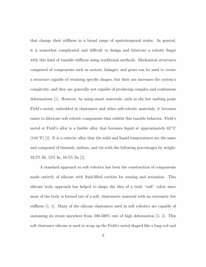
3.3.2 Sample B

Sample B used the silicone compound with less viscosity and strength was used

(Ecoflex 00-50). Two Ni-Cr layers positioning above and below the metal layer were

used as heaters to melt the Field’s metal rods globally. One thermocouple glass braid

was embedded to measure the temperature.

For manufacturing it, one Ni-Cr layer is placed in the acrylic mold, and a little

amount of silicone compound is poured and spread out evenly to be 1-2mm height.

Two Field’s metal rods with approximately 10-11mm gap are laid on the Ni-Cr layer,

and another amount of silicone compound is added to let the metal rods sink with

1-2mm height. After it is cured, the second Ni-Cr layer is placed on it and poured

the little amount of silicone compound again. For the final step, the top surface layer

is put on the second Ni-Cr layer and let them be cured with the silicone compound.

When all layers are completely cured with the silicone compound, the silicone walls

are detached to get sample B.

The sheaths for penetrating thread by the 3d printer are inserted into the holes

on the top layer. One end of the thread is tied up to M3× 6 bolt, and it is fixed on

the end of the sheath. The wire of thermocouple glass braids is also out of the body

and the Ni-Cr wire connects to the bare copper wire.

23

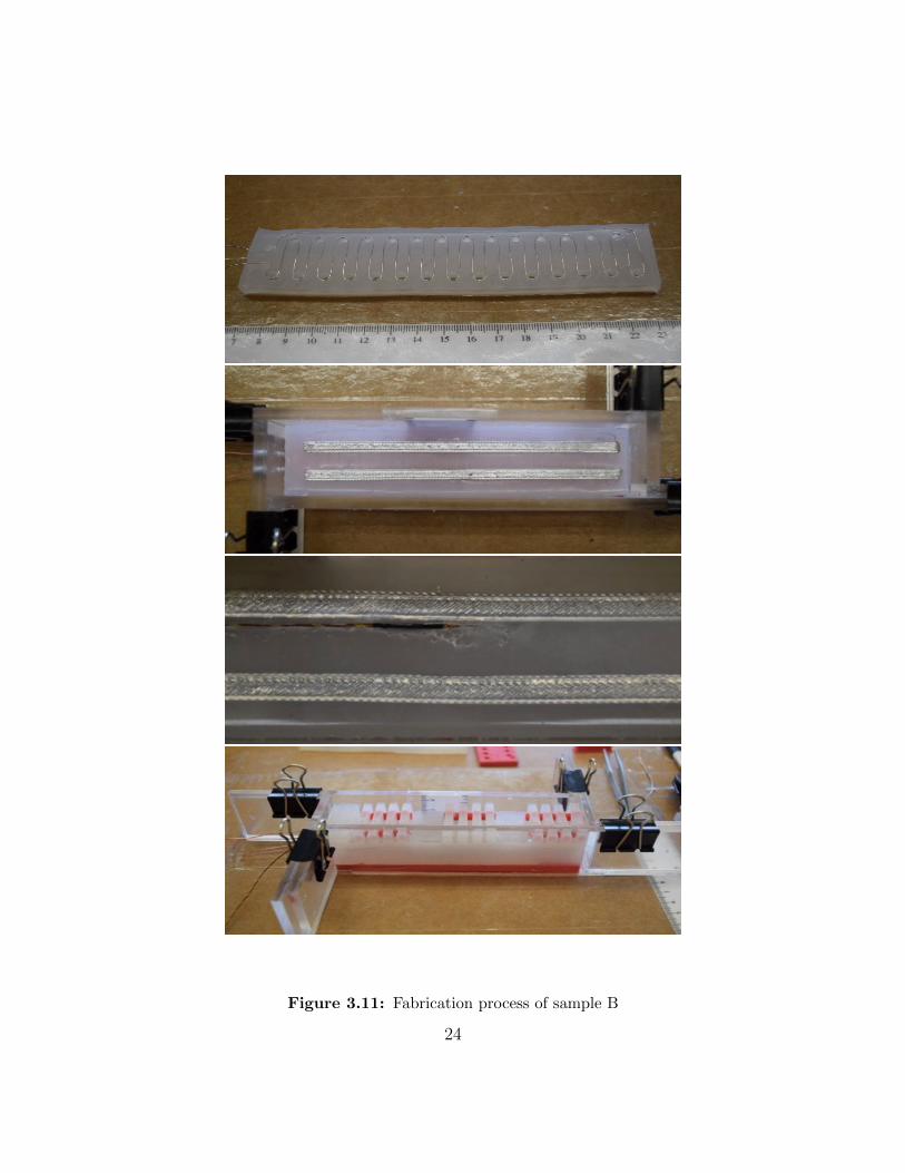
Figure 3.11: Fabrication process of sample B

24

Finally constructed finger devices have 35 × 30 × 172mm size as presented in

Figure 3.12.

Figure 3.12: Completion of sample A (top) and B (bottom)

25

CHAPTER 4. EXPERIMENTS

In order to conduct experiments, the test setup was configured with a power

supply device, thermocouple amplifiers, a Chipkit uC32 board, and a laptop to run the

Arduino code to observe the temperature variation on every second as seen in Figure

4.1. The experiments are mainly to figure out the following points and conducted for

each finger samples independently.

• The time required to reach the melting point (62 ◦C)

• The temperature fluctuation required from the biasing point to achieve localize

or global melting

• The measured thermocouple temperature that corresponds to liquefaction and

solidification of the metal

• Demonstration of local or global stiffness changes

First, it is supposed to measure how long the device takes to bias the tem-

perature up to the melting point, 62 ◦C. Secondly, it is to measure how fast the

temperature goes above and below the melting point. This experiment allows us to

understand that the rate at which the device can vary from its stiff to compliant

regimes and vice versa. Third, it is to figure out accurate temperature to melt down26

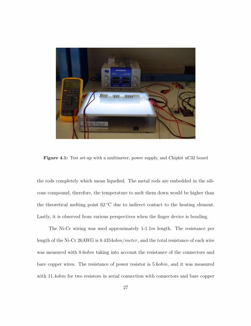
Figure 4.1: Test set-up with a multimeter, power supply, and Chipkit uC32 board

the rods completely which mean liquefied. The metal rods are embedded in the sili-

cone compound, therefore, the temperature to melt them down would be higher than

the theoretical melting point 62 ◦C due to indirect contact to the heating element.

Lastly, it is observed from various perspectives when the finger device is bending.

The Ni-Cr wiring was used approximately 1-1.1m length. The resistance per

length of the Ni-Cr 26AWG is 8.4354ohm/meter, and the total resistance of each wire

was measured with 8.6ohm taking into account the resistance of the connectors and

bare copper wires. The resistance of power resistor is 5.6ohm, and it was measured

with 11.4ohm for two resistors in serial connection with connectors and bare copper

27

wires. The maximum power capacity of each resistor is 5watt. The thermocouple

glass braid wire’s ends were connected to the thermocouple amplifier, which in turn

was analog to digital converter of the Chipkit uC32 board. While running the Arduino

codes for temperature measurement, the power supply was regulated with the voltage

and current. The room temperature was approximately 24 ◦C, and the measurement

started as soon as power supply was switched on.

4.1 Rate of Change of Temperature from 24 ◦C to 62 ◦C

The purpose of this experiment is to figure out how fast the temperature can

reach the actual melting point, 62 ◦C and how the rate of temperature change will be

presented.

4.1.1 Sample A

Sample A was planted with two thermocouple glass braids as seen in Figure

3.8 and it was measured for each point with different power supply. At first, both

heating elements were supplied with maximum electric power and then Ni-Cr wire was

powered only. When dual heaters were used, the starting temperature was 27.5 ◦C

and for the single heater, it was started from 28 ◦C and reached 28.5 ◦C after the 50s.

28

0 100 200 300 400 500 600 700 800 90025

30

35

40

45

50

55

60

65

Time[s]

Tem

per

ature

[◦C

]

Sample A - Rate of Temp. Change to 62 ◦C

Single Heater (Only NiCr wire)Dual Heater (NiCr + Resistors)

4.1.2 Sample B

In the case of sample B, only one thermocouple glass braid was implanted

because it has one kind of heating elements layered up and down to deliver the heat

globally. The first measurement was done with the electric power 8.4watt(1.0A, 8.4V )

for each Ni-Cr wire and the second one done with reduced power to 4.2watt.

29

0 100 200 300 400 500 600 700 800 90025

30

35

40

45

50

55

60

65

Time[s]

Tem

per

ature

[◦C

]

Sample B - Rate of Temp. Change to 62 ◦C

Each NiCr w/ 4.2wattEach NiCr w/ 8.4watt

4.2 Fluctuation of Temperature between 50 ◦C and 70 ◦C

Assuming the temperature area for liquefying and solidifying the metal with

50 ◦C and 70 ◦C respectively, the experiment was conducted to figure out how fast

the rate of change of temperature can fluctuate. The power was on and off repetitively

for increasing and decreasing the temperature within the range.

30

4.2.1 Sample A

For sample A, it was measured at only the point where the thermocouple glass

braid is planted near both Ni-Cr wire and resistor because it is considered as a joint

area of finger device.

0 400 800 1,200 1,600 2,00040

45

50

55

60

65

70

75

80

Time[s]

Tem

per

ature

[◦C

]

Sample A - Fluctuation between 50 ◦C and 70 ◦C

Dual Heater (NiCr + Resistors)

4.2.2 Sample B

As seen in below plot, it was measured two cycles under the electric power

8.4watt for each Ni-Cr wire layered above and below the metal rods.

31

0 400 800 1,200 1,600 2,00040

45

50

55

60

65

70

75

80

Time[s]

Tem

per

ature

[◦C

]

Sample B - Fluctuation between 50 ◦C and 70 ◦C

Each NiCr w/ 8.4watt

4.3 The Temperature of Liquefying and Solidifying the Metal

In order to find the actual temperature area to liquefy and solidify the metal

rods, this experiment was conducted. While monitoring the temperature, the finger

kept bending continuously with the maximum power of heaters. The cooling process

was on the same way.

32

4.3.1 Sample A

0 200 400 600 800 1,000 1,20030

40

50

60

70

80

90

100

110

120

130

140

150

Time[s]

Tem

per

ature

[◦C

]Sample A - Liquefying Temperature

Dual Heater (NiCr + Resistors) On

0 200 400 600 800 1,000 1,20030

35

40

45

50

55

60

65

70

75

80

85

90

Time[s]

Tem

per

ature

[◦C

]

Sample A - Solidifying Temperature

Dual Heater (NiCr + Resistors) Off

33

4.3.2 Sample B

0 200 400 600 800 1,000 1,20030

40

50

60

70

80

90

100

110

120

130

140

150

Time[s]

Tem

per

ature

[◦C

]Sample B - Liquefying Temperature

Each NiCr w/ 8.4watt

0 200 400 600 800 1,000 1,20030

35

40

45

50

55

60

65

70

75

80

85

90

Time[s]

Tem

per

ature

[◦C

]

Sample B - Solidifying Temperature

Each NiCr w/o 8.4watt

34

4.4 Device Actuation and Kinematics

The final aspect of the tunably-compliant fingers is the ability to control both

the melting of the skeleton, either at specific locations within the device or globally

and to cause bending using the tendon routed through the device. In sample A,

shown in Figure 4.2-(Top), the bending is concentrated at the spatial location where

the power resistors have caused localized melting of the Field’s metal skeleton. In

contrast, sample B, shown in Figure 4.2-(Bottom), the bending is continuous across

the entire device as the heating has caused global melting of the Field’s metal skeleton.

Another difference between the two samples was the required force for deformation.

Because sample B was fabricated with the less stiff Ecoflex 00-50 silicone rubber,

the tendon forces required to deform the finger were less than the forces required for

sample A.

From the standpoint of the kinematics of the devices, sample B could be de-

scribed using standard models for large-deflection of highly elastic beams. On the

other hand, devices like sample A where the bending is concentrated in small re-

gions of the total device, simplified models of compliant mechanism as pin joints with

torsional springs can be applied [24].

35

Figure 4.2: Segmented bending with localized heating of sample A (Top). Continuous

bending with global heating of sample B (Bottom)

36

CHAPTER 5. THERMAL ANALYSIS AND SIMULATION

Apart from the direct measurement by the experiments with samples, it is

important to use the thermal analysis and simulation because it can predict the tem-

perature in advance before the sample is designed and manufactured. This chapter

presents the thermal analysis of the device with some equations in thermodynamics

and applied them into the sample A. Also, thermal simulation by the program, Solid-

works (Dassault Systems, Waltham, Massachusetts, USA) is done for the transient

thermal behavior of using each material’s thermal properties. Before the simulation

by the program, the theoretical thermal calculation was done first. The steady state

behavior of the materials was calculated using the thermal mechanism by which heat

is transferred such as conduction and convection. In here, only thermal resistance

by conduction and convection was considered. The thermal resistance R for heat

transfer is defined as the ratio of the change in temperature difference to the change

in heat flow rate [25].

R =dT

dqh(5.1)

The thermal resistance R has units of K·s/J , ◦C·s/J , or ◦F·s/(ft·lb). For simple

one-dimensional conduction can be given by the law of heat conduction

37

qh = kA∆T

L= kA

T1 − T2L

(5.2)

Figure 5.1: One-dimensional conduction heat flow

In Figure 5.1, L is the length of the body, A is the cross-sectional area normal

to the heat flow direction, ∆T is the temperature difference along the length, and k

is the thermal conductivity of the material in W/(m·K) or W/(m· ◦C). Combining

5.1 and 5.2 can give the thermal resistance for conduction like below [25].

R =L

kA(5.3)

For convective heat transfer, the rate of heat flow of the body is proportional

to the difference in temperature between the body and its environment. Therefore,

the mathematical expression can be given as

38

qh = hA∆T = hA(Tsur − Tenv) (5.4)

where A is the surface area, from which the heat is transferred, Tsur is the temperature

of the body surface, Tenv is the temperature of the environment, and h is the heat

transfer coefficient in W/(m2·K) or W/(m2· ◦C). Combining 5.1 and 5.4 can give the

thermal resistance for convection like following.

R =1

hA(5.5)

It is useful to utilize the concept of thermal resistance and represent heat transfer

by a thermal circuit such that the heat flow rate qh is analogous to the current, the

temperature difference ∆T is considered as the voltage, and the thermal resistance can

be the electric resistance. For the composite slab with the thermal resistance in series

interconnection R1 and R2 can be resulted with T1 − T2 = R1qh and T2 − T3 = R2qh

respectively. The total temperature difference across the composite slab is T1 − T3 =

(R1 + R2)qh. Thus, the equivalent thermal resistance for a series interconnection is

like following [25].

Req = R1 +R2 (5.6)

39

Item Thermal Conductivity Specific Heat Mass Density

Unit W/(m ·K) J/(kg ·K) kg/m3

Field’s Metal 18.5 285 7888.77

NiCr wire 11.3 450 8400

Hot End Resistor 1.5 877.96 2300

Silicone Rubber 1.2 1175 1700

Table 5.1: Each material’s properties

5.1 Thermal Analysis of the Steady State Behavior

With above concept, using the section view of sample A as shown in Figure

5.2, the little size of red squares can be considered and also calculated with the

cross-sectional area of each wall and the thickness of each wall. Therefore, it can be

represented using a thermal circuit with five thermal resistances connected in series

as shown in Figure 5.3. First, each cross-sectional area is calculated with the length

of the hot end resistor 7.2mm and the same length of the square 3mm. Therefore,

the cross-sectional area is that 0.0072m × 0.003m = 2.16 × 10−5m2. The thermal

properties of each material are shown in table 5.1. Therefore, the calculation of each

wall’s thermal resistance can be calculated like below.

40

Figure 5.2: Section view of sample A

• R1 = L1/(k1 × A) = 0.00275/(1.5× 2.16× 10−5) = 848.765Ks/J

• R2 = L2/(k2 × A) = 0.00265/(1.2× 2.16× 10−5) = 1022.377Ks/J

• R3 = L3/(k3 × A) = 0.005/(18.5× 2.16× 10−5) = 125.125Ks/J

• R4 = L4/(k4 × A) = 0.0071/(1.2× 2.16× 10−5) = 2739.198Ks/J

• R5 = 1/(h5 × A) = 1/(2731.5× 2.16× 10−5) = 169.490Ks/J

From R1 to R4 is the heat transfer by the conduction with thermal conductivity

of k1, k2, k3, and k4 and the last R5 is the heat transfer by the convection of the air’s

convection coefficient 10W/m2 ·◦ C(= 2731.5W/m2 ·K). According to the equation

5.6, the total thermal resistance is41

Figure 5.3: The thermal resistances circuit for the heat transfer

Req =5∑

i=1

Ri = 4904.955Ks/J

Thus, the heat flow rate from T1 = 100 ◦C to T2 = 25 ◦C through the insulated wall

is

qh =∆T

Req

=(373.15K − 298.15K)

4904.955Ks/J= 0.0153W

The heat flow rate stays the same through the insulated wall. Thus, from left to

right, the heat flow rate through each layer is

42

Resister : qh =(T1 − T3)

R1

⇒ T3 = 360.17K(87.0 ◦C)

Elastomer : qh =(T3 − T4)

R2

⇒ T4 = 344.54K(71.4 ◦C)

Metal : qh =(T4 − T5)

R3

⇒ T5 = 342.63K(69.5 ◦C)

Elastomer : qh =(T5 − T6)

R4

⇒ T6 = 300.74K(27.6 ◦C)

Air : qh =(T6 − T2)

R5

⇒ T2 = 298.15K(25.0 ◦C)

From the above, the temperature from the initial heat source is reduced by each

material’s thermal resistance such as T1 = 100 ◦C→ T3 = 87.0 ◦C→ T4 = 71.4 ◦C→

T5 = 69.5 ◦C→ T6 = 27.6 ◦C→ T2 = 25 ◦C.

In order to figure out the temperature tendency in the device over time, the

thermal flow should be analyzed based on the first law of thermodynamics. For a

system with well-defined boundaries, the law of energy conservation states

∆E = Q−W (5.7)

∆E is the change in energy of the system, Q is the heat flow into or out of the system,

and W is the work done by or on the system [25]. In actuality, the net amount of43

energy added to the system is equal to the net increase in the energy stored internally

in the system and any change in the mechanical energy of the system’s center of mass,

∆E = ∆U + ∆MEC (5.8)

U is the internal thermal energy stored at the molecular level and MEC stands for the

mechanical energy including the kinetic and the potential energy associated with the

system’s mass center. For the systems with negligible change in mechanical energy,

∆U = Q−W = (Qin −Qout)− (Wout −Win) (5.9)

which is the mathematical expression of the first law of thermodynamics. For thermal

systems with pure heat transfer and no work involved, that is Win = Wout = 0, the

law of energy conservation can be presented as

∆U = Q = Qin −Qout (5.10)

or

dU

dt= qhi − qho (5.11)

where qh = dQ/dt is the heat flow rate having units of J/s, which is a watt or

ft·lb/s [25].

44

There is another important concept of the thermal calculation. It is the thermal

capacitance C which is the measure of the heat required to increase the temperature

of the object by a certain temperature interval. It is defined as the ratio of the change

in heat flow to the change in the object’s temperature.

C =dQ

dT(5.12)

where C has units of J/K, J/◦C, or ft · lb/◦F. For a constant-volume process, if it

is assumed that no work is involved and all the heat goes into the internal energy of

the substance,

Q = ∆U = mcv∆T (5.13)

m is the mass of the substance, cv is the constant-volume specific heat capacity of the

substance in units of J ·K/kg, J ·◦ C/kg, or ft · lb◦ · F/slug, and ∆T is the change

in temperature of the substance. Combining Equation 5.12 with Equation 5.13 and

assuming that the density and the volume of the mass are ρ and V , respectively, it is

given such as,

C = mcv = mc = ρV c (5.14)

where c is the specific heat capacity depending on the substance of the object itself,

whereas the thermal capacitance C can be proportional to the mass of the object [25].45

5.2 Thermal Analysis of Transient Behavior

Using the Equation 5.11 and 5.14 above, the differential equation relating the

temperature of very near the heater’s surface T1 and the temperature of very near

the metal’s surface T2 can be derived as shown in figure 5.4.

Figure 5.4: Temperature dynamics of a heated object

Applying the law of conservative of energy to the elastomer, it is

dU

dt= qhi − qho

where U = mcT2 = ρV cT2, and we have

dU

dt=

d

dt(ρV cT2) = ρV c

dT2dt

46

The heat flow rate from the heater to the elastomer qhi is represented like below

and the heat flow rate on the opposite way (out of the elastomer) qho = 0.

qhi =T1 − T2R2

where R2 is the thermal resistance of the elastomer. Thus, the differential equation

becomes

ρV cdT2dt

=T1 − T2R2

Because of the energy flows to the elastomer, ρV c represents the thermal capac-

itance of the elastomer like ρV c = C2. Therefore, the differential equation is finally

obtained as

R2C2dT2dt

+ T2 = T1

In order to calculate the thermal capacitance C2, the density of the elastomer

ρ = 1700kg/m3, the volume of the orange–colored rectangular V = 0.00265m ×

0.001m× 0.0072m = 1.908× 10−8m3, and the specific heat capacity of the elastomer

c = 1175J/kg ·K are applied, therefore

C2 = ρV c = 1700× (1.908× 10−8)× 1175 = 0.0381J/K

47

Also, the thermal resistance of the elastomer R2 can be calculated with the

thermal conductivity k2 = 1.2W/m · K, the cross–sectional area A = 0.0072m ×

0.001m = 7.2× 10−6m2, and the length L2 = 0.00265m,

R2 =0.00265

1.2× (7.2× 10−6)= 306.71Ks/J

Applying C2 = 0.0381J/K and R2 = 306.71Ks/J , the differential equation is clarified

like following.

11.685651s× dT2dt

+ T2 = T1

The equation can be once more clarified for the temperature of near the metal’s

surface T2 such as

T2(t) = T1 − constant× e−0.08557504×t

.

From the above equation, the initial temperature of T2 needs to be the room

temperature 25◦C whatsoever the temperature of the heater T1 will be at the initial

time t = 0s. Let’s have an example that T1 = 75◦C and T2 = 25◦C at t = 0s. Then,

the constant can be calculated like T2−T1 = 25− 75 = −50. Therefore, the equation

in this case becomes

48

T2(t) = 75◦C− 50× e−0.08557504×t

With the time period from 0s to 160s, the thermal analysis of T2 shows the plot of

the red colored curve. The analysis result is approaching to the target temperature

with very steep slope and it does not show very accurate tendency on the simulation

result and the real experimental measurement. However, there were few factors to

be considered such that this calculation just assumed to have only one heater like

the hot end resistor and the thermal properties of the materials would be inaccurate

when compared to the materials used in real. Nonetheless, it is a meaningful process

to establish the thermal modeling and to derive the differential equations.

0 20 40 60 80 100 120 140 16020

30

40

50

60

70

80

Time[s]

T2[◦

C]

Thermal analysis curve of sample A

Thermal analysisThermal simulationExperiment result

49

5.3 Thermal Simulation Using Solidworks FEA

Beside of the thermal calculation, the thermal simulation was conducted to find

out the transient behavior over time and also figure out whether the simulation will be

matched with the experiment curve. Although the thermal conductivity of elastomer

was reported as 1.2W/mK, it was varied and applied to iterate the simulation and

find the good matching curve. The sample device was designed as shown in Figure

5.5 and the Ni-Cr wiring was replaced with the plate type instead of the real one due

to the complexity of the Ni-Cr wiring design. However, the heat power was used the

same value 8.6watt. Also, the heat power of the hot end resistors was applied totally

6.99watt. The purpose of this simulation is to compare the fluctuation of the rate of

the temperature from 50 ◦C to 70 ◦C by the heat power on and off.

Figure 5.5: Model design of sample A(left) and B(right)

50

5.3.1 Simulation to Increase the Temperature to 70 ◦C

0 20 40 60 80 100 120 140 16030

40

50

60

70

80

90

Time[s]

Tem

per

ature

[◦C

]Sample A: Increase the temp. to 70 ◦C

3.4Exp.

This is the first plot of increasing temperature for sample A which has the hot

end resistors and one Ni-Cr layer. The total time lapse was applied with 160s when

the real sample was reached to 70 ◦C. The initial temperature was set up with 32 ◦C

being measured as the starting value of the real experiment. The simulation curve

was almost matched with the experiment curve when the thermal conductivity of

elastomer was set to 3.4W/mK. At the beginning of the curve, it observed somewhat

steeper increase than the experimental one (red color).

51

0 50 100 150 200 250 300 350 40030

40

50

60

70

80

90

Time[s]

Tem

per

ature

[◦C

]

Sample B: Increase the temp. to 70 ◦C

5.0Exp.

In the case of sample B, it should have applied with much more time like 400s

than sample A to get reached 70 ◦C from the room temperature. When sample B

was simulated with the same thermal conductivity value of sample A, the rate of

temperature in the simulation was observed with much higher than the experiment

curve because of the long simulation time period and different heating method such

as the Ni-Cr plates. After iterating the simulation with various values of the thermal

conductivity, it was finally shown matched like above with the value of 5.0W/mK.

52

5.3.2 Simulation to Decrease the Temperature to 50 ◦C

0 20 40 60 80 100 120 140 16030

40

50

60

70

80

90

Time[s]

Tem

per

ature

[◦C

]Sample A: Decrease the temp. to 50 ◦C

3.4Exp.

After increasing the temperature for 160s with the heat powers of both resistors

and Ni-Cr plate, the thermal loads were turned off and it was simulated to know

the decreasing rate of the temperature for another 160s set-up because the cooling

time from 70 ◦C to 50 ◦C was taken with 160s in the experiment. The previous

thermal study by the program was connected to this second simulation, so the initial

temperature was set to start from the highest temperature of the first increasing case.

As shown in the above plot, it showed a tendency to decrease a little bit steep at the

beginning and followed the experiment curve.

53

0 100 200 300 400 500 600 700 81720

30

40

50

60

70

80

90

Time[s]

Tem

per

ature

[◦C

]

Sample B: Decrease the temp. to 50 ◦C

5.0Exp.

For sample B, the simulation was done with the thermal loads off and applied

with the time of 817s taken for cooling down to 50 ◦C in the experiment. The simula-

tion showed that the temperature was uniformly decreased. On the other hand, the

experiment curve started a little bit steeper rate of the temperature change than the

simulation at the beginning and showed the different curve in the middle from 60 ◦C

to 55 ◦C. The intermediate different temperature change is regarded as the transition

from the liquid to the solid state.

54

5.3.3 Simulation to Increase the Temperature to 70 ◦C Again

0 20 40 60 80 10730

40

50

60

70

80

90

Time[s]

Tem

per

ature

[◦C

]Sample A: Increase the temp. to 70 ◦C again

3.4Exp.

For the second cycle of sample A, the thermal loads were turned on again and

it simulated for 107s taken in the experiment to reach 70 ◦C. The reason why shorter

time was taken might be that some heat still existed inside the sample after cooling

down to 50 ◦C in the experiment. For the second temperature increase, as well, it

was connected from the previous cooling down study in order to keep the continuous

temperature fluctuation. As seen on plot, the simulation curve started with some gap

from the experiment curve but was eventually finalized with the match.

55

0 50 100 150 200 250 300 35720

30

40

50

60

70

80

90

Time[s]

Tem

per

ature

[◦C

]

Sample B: Increase the temp. to 70 ◦C again

5.0Exp.

This is also the second temperature increase for sample B and as seen in above,

it showed very good matching between the simulation and the experiment curve

with the thermal conductivity of elastomer 5.0W/mK. It was also connected to the

previous simulation and the initial temperature was set up with the lowest one of the

first decreasing case. The simulation time was applied with 357s as the experiment

was taken.

56

5.3.4 Simulation to Decrease the Temperature to 50 ◦C Again

0 20 40 60 80 100 120 140 160 180 200 22430

40

50

60

70

80

90

Time[s]

Tem

per

ature

[◦C

]Sample A: Decrease the temp. to 50 ◦C again

3.4Exp.

After reaching 70 ◦C in the second increase, the thermal loads were turned off

again and cooled down the device during the time of 224s because it was measured

with the same time period to decrease from 70 ◦C to 50 ◦C in the experiment. Also,

the simulation was connected to the previous thermal study of the second increase for

the continuous temperature fluctuation. The plot started with a little bit difference

but soon followed the experiment curve over time as shown above.

57

0 80 160 240 320 400 480 560 64068220

30

40

50

60

70

80

90

Time[s]

Tem

per

ature

[◦C

]

Sample B: Decrease the temp. to 50 ◦C again

5.0Exp.

This is the second decrease of sample B that turned off all thermal loads again.

In this simulation, it was done for 682s of the time when this process of cooling down

was taken in the experiment. The tendency of simulation curve was similar to the

first decreasing case which fell down evenly. The experiment curve had three steps

in the cooling process and the different curve in the middle is also regarded as the

transition process of the Field’s metal state.

58

5.3.5 Simulation vs. Experiment

0 80 160 240 320 400 480 560 65120

30

40

50

60

70

80

90

100

Time[s]

Tem

per

ature

[◦C

]Sample A: Fluctuation of Temp. at 50 ◦C and 70 ◦C

3.4Exp.

Lastly, the simulation results of each heating and cooling process for sample A

were integrated and presented as one curve. In the experiment, the heating sources

were powered on and off electrically in order to observe how fast the temperature could

go up and down with the specific range of 50 ◦C and 70 ◦C. This way of switching

on and off was also used in the simulation. As the result of it, when the thermal

conductivity of the elastomer was set to 3.4W/mK, it showed that the simulation of

sample A well followed the experiment curve in the fluctuation.

59

0 400 800 1,200 1,600 2,0002,25720

30

40

50

60

70

80

90

Time[s]

Tem

per

ature

[◦C

]

Sample B: Fluctuation of Temp. at 50 ◦C and 70 ◦C

5.0Exp.

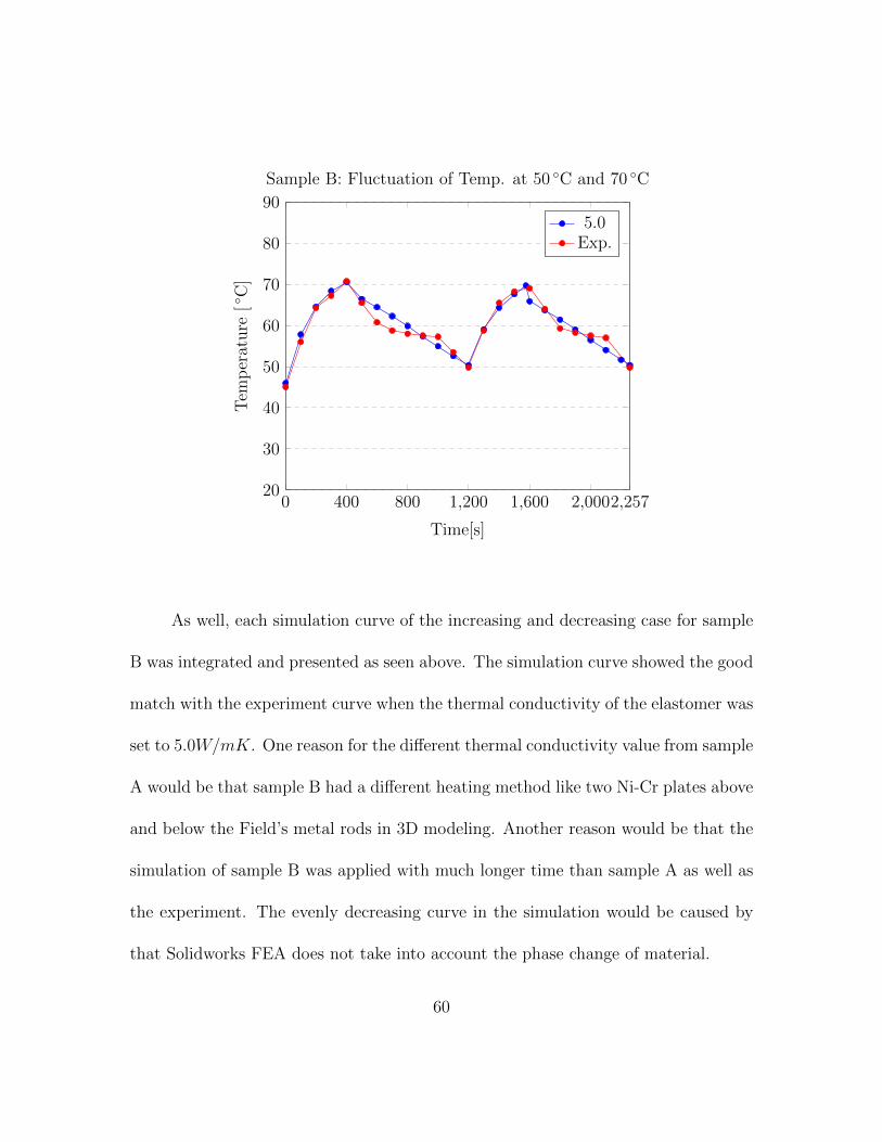
As well, each simulation curve of the increasing and decreasing case for sample

B was integrated and presented as seen above. The simulation curve showed the good

match with the experiment curve when the thermal conductivity of the elastomer was

set to 5.0W/mK. One reason for the different thermal conductivity value from sample

A would be that sample B had a different heating method like two Ni-Cr plates above

and below the Field’s metal rods in 3D modeling. Another reason would be that the

simulation of sample B was applied with much longer time than sample A as well as

the experiment. The evenly decreasing curve in the simulation would be caused by

that Solidworks FEA does not take into account the phase change of material.

60

CHAPTER 6. ADDITIONAL GEOMETRIC

COMPLEXITY OF THE METAL SKELETON

The idea of using the low melting point metal, the various shape of the heating

element, and manipulation by the tendon can be expanded to the more complex

skeletal structure in order to make the device’s motion more degrees of freedom.

Figure 6.1: More complex skeletal structure like lattice

61

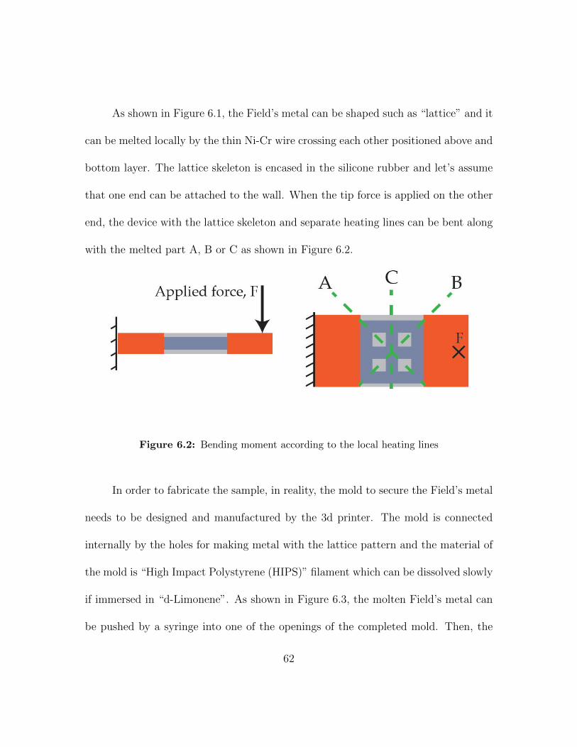
As shown in Figure 6.1, the Field’s metal can be shaped such as “lattice” and it

can be melted locally by the thin Ni-Cr wire crossing each other positioned above and

bottom layer. The lattice skeleton is encased in the silicone rubber and let’s assume

that one end can be attached to the wall. When the tip force is applied on the other

end, the device with the lattice skeleton and separate heating lines can be bent along

with the melted part A, B or C as shown in Figure 6.2.

Figure 6.2: Bending moment according to the local heating lines

In order to fabricate the sample, in reality, the mold to secure the Field’s metal

needs to be designed and manufactured by the 3d printer. The mold is connected

internally by the holes for making metal with the lattice pattern and the material of

the mold is “High Impact Polystyrene (HIPS)” filament which can be dissolved slowly

if immersed in “d-Limonene”. As shown in Figure 6.3, the molten Field’s metal can

be pushed by a syringe into one of the openings of the completed mold. Then, the

62

mold body is supposed to be dissolved by d-Limonene while putting in the beaker.

After removing the mold completely, the Field’s metal skeleton can be washed and

encased in another mold with the silicone rubber solution. The red mold was designed

to fix the Ni-Cr wire positioned up and down through the very small holes keeping

the distance from the metal structure layer by layer. When the silicone rubber is

totally secured, then the sample can be obtained as seen in left, Figure 6.4.

Figure 6.3: Fabrication process of lattice structure sample

63

Figure 6.4 shows that the flat lattice-shaped Field’s metal structure in the rub-

ber can be bent when the only upper Ni-Cr wire was heated. If this unit skeletal

structure is connected in series and the heating position can be controlled freely

where it is supposed to be melted, the whole device can be manipulated much more

degree of freedom. The device can also be applied with the different skeletal structure

or another smart material such as “Nitinol alloy” known as the shape memory alloy.

Figure 6.4: Sample of more complex structure and its bending moment

64

CHAPTER 7. RESULTS AND DISCUSSION

From the experiments of section 4, the first result of increasing to 62 ◦C for

sample A gives that the rate of change of temperature at dual heating elements was

faster than single heating element as expected. In comparison between sample A and

B, despite using different silicone rubber material, sample A with the power resistors

and the Ni-Cr wire was the much faster rate of change than sample B because of

higher and more concentrative thermal energy. In order to reach the melting point

of 62 ◦C, sample A took 104s with the dual heaters and 292s with only Ni-Cr wire

respectively, and sample B took 340s with both Ni-Cr wires of 8.4watt and 827s using

both Ni-Cr wires with half of the full power, 4.2watt. The reason why sample A took

a little shorter time with only one Ni-Cr wire than sample B with both Ni-Cr wires

above and below might be that they didn’t use the same rubber material and the

difference of each elastomer’s thermal conductivity would influence on it.

In the experiment of fluctuation from 50 ◦C to 70 ◦C by powered on and off repet-

itively, sample A showed a much steeper gradient in both increasing and decreasing

temperature than sample B. It took approximately 150s for both heating and cooling

process. On the other hand, sample B consumed more time to raise up to 70 ◦C

and even much more time to lower the temperature 50 ◦C. This results confirmed

65

again that the system delivering the high heat intensively from the combination of

two resistors and one Ni-Cr wire was more efficient than the system delivering the

heat homogeneously from only Ni-Cr wire covering the entire metal rods. As another

observation, it was found that the decreasing gradient was slightly changed in the

range of 55 ◦C to 60 ◦C from the plot of sample B. And it took 400s to reach 70 ◦C

and 800s to go down 50 ◦C. This phenomenon seems to be the process of material’s

phase change from the liquid to the solid state and the range is regarded from 55 ◦C

to 60 ◦C. Also, this phenomenon revealed only sample B while decreasing from 70 ◦C

to 50 ◦C because sample B had the long time period of the cooling process. On the

other hand, sample A couldn’t be observed such a phase change because of its much

shorter time consumed. The experiment of fluctuation was able to compare the simu-

lation result done by Solidworks FEA. The simulation result of sample A had similar

fluctuation tendency compared to the experiment data with the thermal conductivity

of elastomer 3.4W/mK. Also, sample B showed a good match with the experiment

curve entirely with the thermal conductivity of elastomer 5.0W/mK.

The Field’s metal rods are wrapped by the silicone rubber and don’t have the

direct contact to the heating elements which means that the heat is delivered pen-

etrating through the rubber material. Therefore, the melting point of the metal in

this system is thought that it should be compensated to some extent taking into ac-

count the thermal resistance of the rubber material between the heat source and the

66

metal. With this assumption, the plots for finding the liquefied area in section 4.3

showed that both samples were able to bend fully beyond the actual melting point

62 ◦C. While monitoring the temperature near the metal rod on every second, the

experiment to find the appropriate temperature range for bending smoothly was con-

ducted by pulling the tendon carefully and continuously. In the case of sample A, it

had natural bending motion at the temperature of around 80 ◦C. This can also be

confirmed by thermal analysis of the steady state behavior in section 5.1. The ther-

mocouple glass braid sensor was laid between the resistor and the Field’s metal rod.

From the thermal calculation, when the temperature between the resistor’s surface

T3 = 87 ◦C and the metal’s surface T4 = 71.4 ◦C is around 80 ◦C, then the temper-

ature of metal’s outer surface, T5 becomes 69.5 ◦C which is fulfilled with the actual

melting point, 62 ◦C. Therefore, the proper temperature to move the finger device

without any problem is concluded that at least it should be increased up to 80 ◦C. In

the case of sample B, it took 600s to reach 80 ◦C and also showed the natural motion

of bending at this temperature area. The cooling process of both samples had similar

tendency that there was a change of the rate in decreasing the temperature. This

change of temperature rate was observed in the range of 60 ◦C and 55 ◦C in common.

It is assumed that the temperature range might be for the process of turning the

liquid state into the solid state. Lastly, as seen in Figure 4.2, the finger devices were

tried to bend. With more detailed observation, sample A had a tendency of bending

67

with a little angle sharply. On the other hand, sample B was bent more roundly.

Although both samples did not connect the servo motor system to drive them,

they were tried to pull out by the hand and there was no major difficulty in controlling

the finger device when they were well melted globally or locally. Considering the

existing other types of flexible fingers, it is thought that the controllability of this

finger devices is quite comparable with them.

As lessons learned from the results, first of all, it was realized that the silicone

rubber needs to be enough in its viscosity. Otherwise, the device itself will stretch

down due to its own weight when the Field’s metal rods turn out to the liquid state.

Sample B had such a phenomenon because of the low viscosity of the silicone rubber

compared to sample A. Secondly, it was not easy to cast the Ni-Cr wire to the winding

shape using the Ni-Cr mold while making it perfectly planar because the 26 AWG

Ni-Cr wire is too thick to be easily handled. As the result of it, imperfectly planar

fabrication and its inclusion into the layer would have given the influence in changing

the rate at which the heat diffuses to the low melting point metal. This also caused the

uneven silicone layer thickness and affected to create the inconstant distance between

the Field’s metal rods and Ni-Cr wire. While experimenting, the Field’s metal rods

were oxidized and eventually fractured after the bending motions. This is thought

that the metal rods were not melted unevenly due to this unsophisticated fabrication

skill. Also, it was not easy and even so demanding for the thermocouple sensor to

68

implant near the Field’s metal and not to move it while curing the elastomer rubber

due to the sensor wire’s stiffness. Lastly, handling the silicone compound was not

absolutely comfortable because of its sticky feature, especially, combining two cured

silicone layers needed the skill to remove air bubbles in the uncured silicone compound

used to attach them.

As mentioned, while conducting the experiments, the Field’s metal rods had a

tendency to oxidize when heated quickly, such as blackening the surface of the metal

rods, and this resulted in causing the fracture when the devices were applied the

bending moments during the cooling process. This phenomenon is still an ongoing

and pressing problem to be addressed in future research as any crack in the metal

will cause bending concentration at the point of the fracture even when the metal is

hardened.

69

CHAPTER 8. CONCLUSION

Although there have been many kinds of design and fabrication of robotic finger,

this approach of a monolithic, composited device that can exhibit capabilities of both

soft robotics and traditional rigid-link robotics has the potential of enhancing the

field of soft robotics. The devices are simple to fabricate, and further investigations

of the geometry of the composited smart materials are ongoing. In this thesis, we

just introduced the very basic form of the finger and conducted simple experiments

to identify fabrication techniques and the thermal response of the device. However,

this series of processes and its results could lead us a more advanced step and give

not only other ideas and inspiration but also problems which should be solved.

The specific improvement includes using the Ni-Cr wires solely as a biasing

element to raise the entire device temperature close to the melting point and getting

localized melting (e.g. finger joints) through another local heat source, such as power

resistors. So, the sum of heat by Ni-Cr wire and resistors would be enough to melt

the Field’s metal at specific locations. Additionally, a tendon will be incorporated to

pull the finger while heating. Tendon-based actuation systems have been successfully

used to transmit force/motion in devices in which, because of constraints on inertia

and size, it is necessary to place the motors remotely with respect to the joints [26].

70

This ability to control the stiffness of soft robotic components has the potential

to enhance the field of soft robots, thus allowing soft robots to exert large forces on

environments when necessary, and to withstand external loads while keeping their

shape [27]. By making the finger a variable-stiffness device, the robot hand can grasp

a soft object and can manipulate objects easily with high dexterity by adjusting the

finger softness [28], while maintaining rigidity after a grasp is attained and the device

is cooled.

71

BIBLIOGRAPHY

[1] W. Wang, H. Rodrigue, and S.-H. Ahn, “Smart soft composite actuator withshape retention capability using embedded fusible alloy structures,” Elsevier,Composites Part B: Engineering, vol. 78, pp. 507–514, 2015.

[2] K. A. Shaikh and C. Liu, “A Bi-Stable Latchable PDMS Valve Employing LowMelting Temperature Metal Alloys,” TRANSDUCERS 2007 - 2007 Interna-tional Solid-State Sensors, Actuators and Microsystems Conference, pp. 2199–2202, 2007.

[3] I. Filip, M. A. D., S. R. F., C. Xin, and W. G. M., “Soft Robotics for Chemists,”Angewandte Chemie International Edition, vol. 50, no. 8, pp. 1890–1895, 2011.

[4] R. A. Bilodeau, E. L. White, and R. K. Kramer, “Monolithic fabrication ofsensors and actuators in a soft robotic gripper,” pp. 2324–2329, 2015.

[5] S. Wanliang, T. Lu, and C. Majidi, “Soft-matter composites with electricallytunable elastic rigidity,” IOP, Smart Materials and Structures, vol. 22, no. 8,2013.

[6] G. Tonietti, R. Schiavi, and A. Bicchi, “Design and Control of a Variable Stiff-ness Actuator for Safe and Fast Physical Human/Robot Interaction,” pp. 526–531, 2005.

[7] R. Schiavi, G. Grioli, S. Sen, and A. Bicchi, “VSA-II: a novel prototype of vari-able stiffness actuator for safe and performing robots interacting with humans,”pp. 2171–2176, 2008.

[8] N. G. Tsagarakis, I. Sardellitti, and D. G. Caldwell, “A new variable stiffnessactuator (CompAct-VSA): Design and modeling,” pp. 378–383, 2011.

[9] S. B. Kim, C. Laschi, and B. Trimmer, “Soft robotics: a bioinspired evolutionin robotics,” vol. 31, pp. 287–294, 2013.

[10] S. Kim, C. Laschi, and B. Trimmer, “Soft robotics: a bioinspired evolution inrobotics,” Trends in biotechnology, vol. 31, no. 5, pp. 287–294, 2013.

[11] I. D. Walker and M. W. Hannan, “A novel ’elephant’s trunk’ robot,” vol. 2,pp. 410–415, 1999.

72

[12] M. W. Hannan and I. D. Walker, “Kinematics and the implementation of anelephant’s trunk manipulator and other continuum style robots,” Journal of FieldRobotics, vol. 20, no. 2, pp. 45–63, 2003.

[13] R. F. Shepherd, F. Ilievski, W. Choi, S. A. Morin, A. A. Stokes, A. D. Mazzeo,X. Chen, M. Wang, and G. M. Whitesides, “Multigait soft robot,” vol. 108,pp. 401–403, 2011.

[14] W. McMahan, B. Jones, I. Walker, V. Chitrakaran, A. Seshadri, and D. Daw-son, “Robotic manipulators inspired by cephalopod limbs,” Proceedings of theCanadian Engineering Education Association, 2011.

[15] M. Calisti, M. Giorelli, G. Levy, B. Mazzolai, B. Hochner, C. Laschi, andP. Dario, “An octopus-bioinspired solution to movement and manipulation forsoft robots,” Bioinspiration & biomimetics, vol. 6, no. 3, p. 036002, 2011.

[16] Y.-L. Park, B.-r. Chen, C. Majidi, R. J. Wood, R. Nagpal, and E. Goldfield,“Active modular elastomer sleeve for soft wearable assistance robots,” in Intel-ligent Robots and Systems (IROS), 2012 IEEE/RSJ International Conferenceon, pp. 1595–1602, IEEE, 2012.

[17] J.-y. Nagase, S. Wakimoto, T. Satoh, N. Saga, and K. Suzumori, “Design ofa variable-stiffness robotic hand using pneumatic soft rubber actuators,” SmartMaterials and Structures, vol. 20, no. 10, p. 105015, 2011.

[18] M. C. Yuen, R. A. Bilodeau, and R. K. Kramer, “Active variable stiffness fibersfor multifunctional robotic fabrics,” IEEE Robotics and Automation Letters,vol. 1, no. 2, pp. 708–715, 2016.

[19] L. H. Scarborough, C. D. Rahn, and E. C. Smith, “Fluidic composite tunable vi-bration isolators,” Journal of Vibration and Acoustics, vol. 134, no. 1, p. 011010,2012.

[20] Y. Yang, Y. Chen, Y. Wei, and Y. Li, “Novel Design and Three-DimensionalPrinting of Variable Stiffness Robotic Grippers,” Journal of Mechanisms andRobotics, vol. 8, no. 6, p. 061010, 2016.

[21] V. K. Venkiteswaran and H.-J. Su, “A Three-Spring Pseudorigid-Body Modelfor Soft Joints With Significant Elongation Effects,” Journal of Mechanismsand Robotics, vol. 8, no. 6, p. 061001, 2016.

[22] T. Hassan, M. Manti, G. Passetti, N. d’Elia, M. Cianchetti, and C. Laschi, “De-sign and development of a bio-inspired, under-actuated soft gripper,” pp. 3619–3622, 2015.

73

[23] M. Manti, T. Hassan, G. Passetti, N. dElia, M. Cianchetti, and C. Laschi, AnUnder-Actuated and Adaptable Soft Robotic Gripper, pp. 64–74. 2015.

[24] L. L. Howell, Compliant mechanisms. John Wiley & Sons, 2001.

[25] E. S. Ramin and L. Bei, “Dynamic systems: modeling and analysis,” vol. 2,pp. 316–326, 1995.

[26] G. Palli, G. Borghesan, and C. Melchiorri, “Modeling, identification, and controlof tendon-based actuation systems,” IEEE Transactions on Robotics, vol. 28,no. 2, pp. 277–290, 2012.

[27] J. Shintake, B. Schubert, S. Rosset, H. Shea, and D. Floreano, “Variable stiff-ness actuator for soft robotics using dielectric elastomer and low-melting-pointalloy,” pp. 1097–1102, 2015.

[28] J.-Y. Nagase, S. Wakimoto, T. Satoh, N. Saga, and K. Suzumori, “Design ofa variable-stiffness robotic hand using pneumatic soft rubber actuators,” IOP,Smart Materials and Structures, vol. 20, no. 10, p. 105015, 2011.

74