1

Design and Development of Low cost spirometer with pc Interface

Seakale Chandrakar

A Dissertation Submitted to

Indian Institute of Technology Hyderabad

In Partial Fulfillment of the Requirements for

The Degree of Master of Technology

Department of Electrical Engineering

(Micro Electronics and VLSI Design)

June, 2014

2

Declaration

I declare that this written submission represents my ideas in my own words, and where others’ ideas or

words have been included, I have adequately cited and referenced the original sources. I also declare that

I have adhered to all principles of academic honesty and integrity and have not misrepresented or

fabricated or falsified any idea/data/fact/source in my submission. I understand that any violation of the

above will be a cause for disciplinary action by the Institute and can also evoke penal action from the

sources that have thus not been properly cited, or from whom proper permission has not been taken when

needed.

Seekala Chandrakar

EE12M1032

3

4

Acknowledgements

I would like to take this opportunity to sincerely thank my project guide

Dr. Asudeb Dutta, Professor, Department of ECE, IITHyderabad, for his constant guidance,

encouragement and help during the entire duration of the Project. His enthusiasm has been a driving

force for our efforts through the course of this project.

I express my sincere thanks to Shaik Shabana Project staff and Dr.V.V.Rao Govt. Chest Hospital and

Dr.Anuradha Star Hospital and Dr.Renu John Professor and continuous support in completion of my

project.

Finally, I wish to thank the other staff members and my friends for their help and

encouragement during the execution of this project work.

5

Dedicated to

All my Friends and Family.

6

TABLE OF CONTENTS

Title Page No.

LIST OF FIGURS vii

LIST OF TABLES ix

LIST OF ABBREVIATIONS x

Chapter 1 INTRODUCTION 9

1.1 History of spirometry 9

1.2 Early development of spirometers 13

1.3 Present Technology based Spirometers 14

1.4 Spirometry Monitoring Technology 16

Chapter 2 COPD 17

2.1 What is COPD 17

2.2 Diagnosis 18

2.3 Diagnosis of COPD 19

2.4 Diagnosis criteria 19

2.5 Reference Values 20

2.6 Symptoms of COPD 20

2.7 Development of a definition of COPD 22

2.8 Comparison of definition of COPD 23

2.9 Development of airflow obstruction in COPD 24

2.10 Measurement of ventilator function by spirometry 25

2.11 Classification of abnormal spirometry 26

7

Chapter 3 Spirometry 27

3.1 Measurement Technique 27

3.2 Measurement Variability 28

3.3 Spirometer Parameters 29

3.4 Classification of Parameters 29

3.5 Respiratory Function 30

3.6 Lung-Volume Loop Parameter 31

3.7 Flow-Volume Loop Graph Parameter 33

3.8 Forced Average Expiratory Flow as a Percentage of FVC 33

3.9 Forced Vital Capacity (FVC) 37

3.10 Maximum Mid-Expiratory Flow 38

3.11 Quality of the Spirometry 38

3.12 Quality Test 39

Chapter 4 Spirometer Design 46

4.1 Principles of Operation (Spirometer) 46

4.2 Pressure sensor (Differential Pressure Sensor) 48

4.3 Processing Stage 53

Chapter 5 Sensor Design in COMSOL 54

5.1 Introduction to Sensor Design 54

5.2 Types of Pressure Measurements 55

5.3 Pressure Sensing Technology 56

5.4 Applications 58

Chapter 6 Design of Piezoresistive Pressure Sensor 60

6.1 Introduction 60

8

6.2 Model Definition 60

6.3 Device Physics and Equation 60

6.4 Pressure Sensor Types and Classification 62

6.5 Piezoresistive Transducer Analyses and Design 65

6.6 Sensitivity (S) 66

6.7 Design Concept of Pressure Sensor 69

Chapter 7 Design of CNT Based Pressure sensor 85

7.1 Introduction to CNT Pressure Sensor 85

7.2 CNT Pressure Sensor Model 86

7.3 Piezoresistive of CNT 88

7.4 Results in COMSOL for CNT Pressure sensor 91

Chapter 8 LABVIEW PC Interface 93

8.1 Introduction to LABVIEW 95

8.2 Programming in Lab View 97

8.3 Experimental setup 97

8.4 Results 98

8.5 Discussion and Conclusion 98

8.6 Applications 99

Chapter 9 ADC Design in FPGA 100

9.1 Code for ADC in FPGA 100

Chapter 10 Lung Age Calculation 115

10.1 Introduction to LUNG AGE 116

10.2 Methods for Calculation 119

10.3 Design and Methods 119

10.4 Spirometer function tests 121

10.5 Equation for LUNG AGE 122

References 123

9

Abstract

The primary test of lung function is called Spirometry. Spirometry parameters are derived from pressure

and/or flow measurements. The spirometer records exhaled air volume, and produces graphic and

numeric information in the form of spirometric parameters and tracings that can depict and describe the

mechanical properties of the lung. Some possible measurements are like Pressure and gas flows behave

during one respiratory cycle in volume controlled. Patient Spirometry measures airway pressures, flow,

volumes, compliance, and airway resistance breath-by-breath at the patient’s airway. The flow of gas is

measured, and the inspiratory and expiratory concentrations of oxygen and carbon dioxide analyzed. All

parameters are measured through a single, lightweight flow sensor and gas sampler, placed at the patient’s

airway. The “close to the patient” measurement is a sensitive and continuous reflector of patient’s

ventilator status, obtained independently of the ventilator used. The breath-by-breath measurement of

pulmonary gas exchange is technically very demanding and requires sophisticated compensation and data

processing algorithms to achieve the accuracy required in

the clinical use. Measurement of respiratory gas flow continuously is associated with several problems,

such as the effects of humidity, alternating gas composition, secretions, and the dynamic response of the

flow sensors. Medical technologies have enabled accurate measurement of respiratory gas exchange in a

wide variety of clinical conditions. The clinical applications range from assessment of energy

requirements to comprehensive analysis of ventilation and oxygen transport in patients with complex

cardio respiratory problems. Obstructive disorders, which are much more common than restrictive

abnormalities include asthma and COPD.

Asthmatic bronchitis, chronic bronchitis, and emphysema are included in COPD. These diseases can be

identified by a low FEV / FVC ratio or an FEV that is lower than predicted. Spirometric data have been

presented as exhaled volume over time. These volume-time curves are easy to visualize and allow

physicians to identify FEV, FVC, and expiratory time at a glance. The flow transducer permits physicians

to visualize peak flow and timed peak flow. Which is a check of patients’ efforts FEV, FVC, and FEV,

FVC ratio are expressed in terms of lower limit of normal.

Here the FEV1/FVC ratio is about the same as (i.e., 57% vs. 59%), but the absolute FEV, is only 66% of

predicted. Spirometric measurements can be as fundamental to medicine as are pulse, blood pressure.

Temperature, height and weight measurements and therefore could be considered in the physical

examination as important vital signs.

10

Abbreviations

ACCP American College of Chest Physicians

AEFV area of expiratory flow-volume

ANCOVA analysis of covariance

ATS American Thoracic Society

BMI body mass index

BMRC British Medical Research Council

BTPS body temperature and pressure saturated

CI confidence interval

COPD chronic obstructive pulmonary disease

CoV coefficient of variation

ECCS European Community for Coal and Steel

ECRHS European Community Respiratory Health Survey

ERS European Respiratory Society

ETS environmental tobacco smoke

EV extrapolated volume

FEFx instantaneous forced expiratory flow when x% of the FVC has been

expired

FEF25-75% forced expiratory flow between 25% and 75% of FVC

FET forced expiratory time

FEV1 forced expiratory volume in one second

FEV6 forced expiratory volume in six seconds

FEVt forced expiratory volume in t second(s)

11

FIRS Forum of International Respiratory Societies

FIV1 forced inspiratory volume in one second

FIVC forced inspiratory vital capacity

FRC functional residual capacity

FVC forced vital capacity

FVC6 forced vital capacity in six seconds

GOLD Global Initiative for Chronic Obstructive Lung Disease

HRCT high-resolution computed tomography

IC inspiratory capacity

ICC intraclass correlation coefficient

ICS inhaled corticosteroid

ITS Intermountain Thoracic Society

IUATLD International Union Against Tuberculosis and Lung Disease

IVC inspiratory vital capacity

LLN lower limit of normal

MEFx maximal instantaneous forced expiratory flow where x% of the FVC

remains to be expired

MEFV maximum expiratory flow-volume

MMEF maximum mid-expiratory flow

MSB mean squares between groups

MSW mean squares within a group

OAD obstructive airways disease

OLIN Obstructive Lung Disease in Northern Sweden

12

PAR population attributable risk

PEF peak expiratory flow

PIF peak inspiratory flow

PM1 particulate matter under 10 µm in aerodynamic diameter

RV residual volume

SD standard deviation

TLC total lung capacity

VC vital capacity

VDGF vapours, dusts, gases and fumes

13

CHAPTER 1

INTRODUCTION

1.1 History of spirometry

The earliest attempt for the measurements of lung volumes can be dated back to period

129-200 A.D. Claudius Galen, who was a Roman doctor and philosopher, first did a volumetric

experiment on human ventilation. He had a boy breathe in and out of a bladder and found out

that the volume did not change. The experiment proved inconclusive.1681, Borelli tried to

measure the volume of air inspired in one breath. He assembled a cylindrical tube partially filled

with water, with an open water source entering the bottom of the cylinder. He occluded his

nostrils, inhaled through an outlet at the top of the cylinder, and measured the volume of air

displaced by water. This technique is very important in getting parameters of lung volumes

nowadays.1813; Kentish E used a simple "Pulmometer" to study the effect of diseases on

pulmonary lung volume. He used an inverted graduated bell jar standing in water, with an outlet

at the top of the bell jar controlled by a tap. The volume of air was measured in units of pints.

1831, Thrackrah C.T described the "Pulmometer" similar to that of Kentish. He portrayed the

device as a bell jar with an opening for the air to enter from below. There was no correction for

pressure. Therefore, the spirometer not only measured the respiratory volume, but also the

strength of the respiratory muscles.1845, Vierordt in his book named "Physiologies des Athmens

mit besonderer Rücksicht auf die Auscheidung der Kohlensäure" in which his main interest was

to measure the volume of expiration accurately. However, he also completed accurate measures

of other volume parameters by using his "Expiratory". Some of the parameters described by him

are used today which included residual volume and vital capacity.1846 The water spirometer

measuring vital capacity was developed by a surgeon named John Hutchinson. He invented a

calibrated bell, inverted in water, which was used to capture the volume of air exhaled by a

person. John published his paper about his water spirometer and the measurements he had taken

from over 4,000 subjects, describing the direct relationship between vital capacity and height and

inverse relationship between vital capacity with age. He also showed that vital capacity does not

relate to weight at any given height. He also used his machine for the prediction of premature

mortality. He coined the term vital capacity, which was claimed as a powerful prognosis for

heart disease by Framingham study. He believed that his machine should be used as actuarial

14

predictions for companies selling life insurances.1854 Wintrich developed a spirometer, which

was easier to use than Hutchinson's. He did an experiment with 4,000 experimental subjects, and

concluded that there are 3 parameters affecting vital capacity: body heights, weights and age,

which showed similar results as Hutchinson's study. In 1879, Gad J. published a paper named

"Pneumatograph" which allowed the recording of lung volume changes.1859 E. Smith developed

a portable spirometer, on which he measured gas metabolism.1866 Salter added a kymograph to

the spirometer in order to record time while obtaining air volumes. 1902, Brodie T.G was the

first using a dry-bellowed wedge spirometer. Compton S.D developed the lung meter in 1939

during for use in Nazi Germany. Wright B.M. and McKerrow C.B. introduced the peak flow

meter in 1959. In 1969, DuBois A.B. and van de Woestijne K.P. experimented on humans the

whole body-plethysmograph. In 1974, Campbell et al. refined the previous peak flow meter and

put forward a cheaper and lighter version of a peak flow meter.1904 Tissot introduced the

closed-circuit spirometer.2008 Advanced Medical Engineering developed the world's first

wireless spirometer with 3D Tilt-Sensing for far greater quality control in the testing

environment. A spirometer is an apparatus for measuring the volume of air inspired and expired

by the lungs. A spirometer measures ventilation, the movement of air into and out of the lungs.

The spirometer will identify two different types of abnormal ventilation patterns, obstructive and

restrictive. There are various types of spirometers which use a number of different methods for

measurement (pressure transducers, ultrasonic, water gauge).

A spirometer is used to conduct a set of medical tests that are designed to identify and quantify

defects and abnormalities of various lung conditions in human respiratory system (Fishman,

1998; Hyatt et al., 1997). These tests also help in monitoring the response of lungs to medical

treatment. With the help of a spirometer, Chronic Obstructive Pulmonary Disease (COPD) can

be detected well in advance (American Thoracic Society, 1995a). Monitoring cough and

wheezing may not provide an accurate assessment of the severity of asthma in a patient. With the

help of the breathing tests conducted using a spirometer, the response, and improvement in an

asthma patient’s condition during the treatment can be monitored accurately. This improves the

quality of treatment by reducing the judgment errors. American Thoracic Society (ATS) has

recommended these breathing tests for all those who have a family history of chronic respiratory

illness, cough, or dispend and even for habitual smokers (American Thoracic Society, 1995b). In

fact, this test is mandatory to confirm the physical fitness for entry into government services and

15

the armed forces in many countries. Spirometer measures the flow and volume of gas (air)

moving in and out of the lungs during a breathing maneuver (Downing, 1995).

Fig: Spirometer Types

The measured flow and volume values are plotted as graphs called the spirograms that are used

for diagnosis of the patient. A brief overview of the terms used in these tests, types of spirograms

and the relation between them, is included in a subsequent section. Several methods (Figure 1)

are used to realize spirometers (Fishman, 1998; Weber, 1999). The spirometers are based on the

measurement of either the flow rate or the volume of gas inhaled and exhaled during respiration.

The pressure measurement system depicted in Figure 1(c) is, in fact, also a flow rate

measurement-based method where the flow rate is indirectly determined by measuring the

pressure (e.g., orifice or Ventura tube meters). Few methods reported in the literature to realize

spirometers are briefly discussed in the subsequent sections. Figure 1 various methods of

obtaining spirograms: (a) by volume measurement; (b) by flow rate measurement and (c) by

pressure measurement some of the spirometers are constructed based on magneto-striction

principle. Good quality ferromagnetic material is available for this type of spirometers (Nakesch

and Pfutzner, 1995). These spirometers have advantage in the situation where the sensor is

required to be changed frequently. However, such spirometers have to be calibrated more

frequently (each time the sensor is changed, calibration is required). Further, the relation between

the flow rate and the output voltage is also very complex in these spirometers. Design and

development of a low-cost spirometer. Some other spirometers use direct measurement by

collecting the gas in a container. In these spirometers, the volume collected must be temperature

compensated and the container for collection of the gas should be leak proof and at the same

time should not offer any resistance while breathing. Also, care should be taken regarding the

16

condensed water vapors on the walls of the container. Some spirometers are also developed

using flow time monitor method (Lim et al., 1998). These spirometers have an improved

mouthpiece, which makes them suitable even for pediatric use. A major disadvantage of these

spirometers is that they can be used only in conjunction with a computer or a laptop. Another

drawback of these spirometers is that they use preset pressure transducer switches, so there is no

continuous monitoring of the input signal. Another (digital) spirometer, based on the principle of

hot wire sensor, has been proposed by Lin et al. (1998), This spirometer exhibits good

performance but replacing of sensor is expensive. However, this digital spirometer can be

connected to a nearby computer, which can be very advantageous. Many a times these tests need

to be performed right at the time of the asthma attack. It is very unlikely that a doctor will be

present with the patient at that moment. A possible solution is to embed a web server and make

the device (spirometer) network available for online treatment. Online treatment occupies a

prominent place in today’s world as internet provides access to the data from anywhere in the

world through standard browser technology (Economic et al., 1996). Consulting a specialist, who

is located far away from a patient, can be achieved through the internet (Levy and Lawrence,

1992; Szymanski, 2000). Web server also helps in maintaining and accessing the records of a

patient. As the web servers have become a popular tool for sharing data, this feature may be

embedded into the spirometer (Lovell et al., 2001; Finkelstein et al., 1998). This enables the

spirometer to share the data with a doctor who may be located at a distant place (Levy and

Lawrence, 1992; Szymanski, 2000). By using a web-server-based spirometer, a physician can,

for example perform online dynamic lung function test and obtain the results. Thus, Patient’s test

results (graphs etc.) and symptoms are available online to the doctor. Functionally, an embedded

web server can be as powerful as a full web server. The embedded web server knows all about

the system in which it is embedded. It can provide access to the data and perform tasks as

requested. It can activate routines to interpret the requests and modify applications via a standard

Hyper Text Mark-up Language (HTML) browser. The embedded web server should also have

appropriate signal processing capability (Leung et al., 1998) to deal with the acquired medical

data from tests such as a pulmonary function test. This paper presents the design and

development of a simple, low-cost digital spirometer. A new feature of embedding a web server

in a spirometer is described and implemented in the developed prototype. Spirometers with

computer connectivity are available, but to the best of author’s knowledge, spirometer with

17

embedded web-server technology has not been reported so far. All the details of this work are

presented in the subsequent sections.

1.2 Early development of spirometers:

Turbine Spirometer. Hot wire Spirometer. Pressure sensor Spirometer. Ultrasonic Spirometer.

Fig: Types of Spirometer Modules

Spirometry monitoring can be used in the primary, secondary, and tertiary prevention of

occupational and non-occupational respiratory disease and in the maintenance of workers’

fitness. Primary prevention of occupational respiratory disease through control or elimination of

adverse exposures in the workplace is a priority. With respect to primary prevention, spirometry

monitoring of workers can be used to assess the respiratory health status of subgroups of workers

exposed to a particular agent (or production process) to determine if exposures to that agent (or

production process) is unsafe and needs to be controlled. However, even with exposure controls

in place, some workers may be adversely affected; such residual occupational risks and non-

occupational exposures (e.g., tobacco smoke) provide a role for spirometry monitoring in

secondary and tertiary prevention. With respect to secondary prevention, spirometry can be used

to monitor worker populations exposed to potential respiratory hazards to identify otherwise

18

healthy individuals who are experiencing excessive lung function decline; individualized

preventive intervention can then be applied to prevent further excessive loss and subsequent lung

function impairment. With respect to tertiary prevention, spirometry can be used to carefully

monitor an individual worker with established lung function impairment and/or symptoms as part

of clinical management to help prevent disabling impairment and limit symptoms. Generally,

respiratory disease prevention is best done as part of an overall health maintenance program in

which results of spirometry evaluations are linked with exposure control, smoking cessation, and

general health-promotion interventions. Vital graph has used many different precision

technologies for measuring flows and volumes. In the early days of office spirometry these

included measurement of volume by water displacement and the displacement of volumes by

mechanical movement, including bellows, rolling seals and precision syringes which are still

used as reference devices. Today, flow measuring technology predominates in modern office

spirometers and respiratory monitors because the technologies tend to be less expensive and of

smaller size. Lilly or Fleisch technologies are used in professional grade flow measuring

spirometers. Lilly types, which may be single or multi-screen, are no longer used in vital graph

devices. Stator-rotor devices are used for less robust and accurate devices such as screeners and

monitors. Such devices are also difficult to clean and their limited life makes them unsuitable for

satisfactory spirometry examinations, although they are ideal for screening and are cheap to

replace. Vital graph have used and explored many other flow measuring technologies including

heated pneumotachs, platinum wire anemometers, ultrasonic ‘time of flight’ flow meters, orifice

plates, vortex shedders, variable orifice flow meters and others, many of which can perform well

in metrology laboratory conditions with frequent recalibration and linearity setting, but none of

these perform satisfactorily in the conditions encountered in routine office spirometry.

1.3 Present Technology based Spirometers

The biggest impact comes from the technology that quickly puts the data into the hands of the

physician with easy access at any time. Centralized databases with remote review stations give

the physician the opportunity to access patient data anywhere within the network. The physician

can electronically review, interpret, and sign the report without having to go to a particular test

station, or the need for a printed report.

19

Systems such as LAB VIEW, MATLAB physician review software allow the physician to access

patient data through the Internet. Now the physician can be at home or on the road and access

data from anywhere in the world where the Internet is available. The emphasis on data

management, and what you can do with that data, is the focus for the future. The test devices

themselves will become a smaller part of the patient care continuum.

The greatest challenge in medicine is prevention or early treatment of diseases in order to avoid

premature morbidity and mortality. Hand-in-hand with this aim is avoiding or relieving

physician discomfort. The use of spirometry, simple office-based lung function testing, can

identify patients who are often asymptomatic but risk suffering or death from disabling or fatal

diseases, such as lung cancer heart attack and stroke as well as premature deaths from all causes.

Spirometry is especially valuable in early detection of chronic obstructive pulmonary disease

(COPD).This article describes the essential features of spirometry in clinical relevant terms and

explains why practicing physicians should make spriometric evaluation an essential part of

patient examinations, particularly for those at risk of pulmonary disease.

The technology advancements in the category run the gamut from improved workflow to the

digital harvest of patient information. What’s more, mobile technology has revolutionized

spirometers and pulmonary function testing, and, for many in the industry, it’s only just

beginning. RT Magazine asked four leading manufacturers their thoughts on the segment, and

their responses were as varied as the technology they provide. The values measured in

spirometry and pulmonary functions have, for the most part, remained the same for a number of

years. The introduction of a number of measurement transducers based on flow has succeeded in

introducing spirometry to areas that were not previously hospital-based. This has made

diagnosing obstructive disease in primary care offices, with referrals to PFT labs, more common.

Additionally, electronic or digital communication of patient data has grown and will continue to

do so at a faster rate in the future because of advances in connectivity.

20

1.4 Spirometry Monitoring Technology:

Spirometry monitoring can be used in the primary, secondary, and tertiary prevention of

occupational and non-occupational respiratory disease and in the maintenance of workers’

fitness. Primary prevention of occupational respiratory disease through control or elimination of

adverse exposures in the workplace is a priority. With respect to primary prevention, spirometry

monitoring of workers can be used to assess the respiratory health status of subgroups of workers

exposed to a particular agent (or production process) to determine if exposures to that agent (or

production process) is unsafe and needs to be controlled. However, even with exposure controls

in place, some workers may be adversely affected; such residual occupational risks and non-

occupational exposures (e.g., tobacco smoke) provide a role for spirometry monitoring in

secondary and tertiary prevention. With respect to secondary prevention, spirometry can be used

to monitor worker populations exposed to potential respiratory hazards to identify otherwise

healthy individuals who are experiencing excessive lung function decline; individualized

preventive intervention can then be applied to prevent further excessive loss and subsequent lung

function impairment. With respect to tertiary prevention, spirometry can be used to carefully

monitor an individual worker with established lung function impairment and/or symptoms as part

of clinical management to help prevent disabling impairment and limit symptoms. Generally,

respiratory disease prevention is best done as part of an overall health maintenance program in

which results of spirometry evaluations are linked with exposure control, smoking cessation, and

general health-promotion interventions.

21

Chapter 2

Chronic obstructive pulmonary disease (COPD)

2.1 What is COPD?

Chronic obstructive pulmonary disease (COPD) is a preventable and treatable disease

characterized by chronic airflow limitation that is not fully reversible. This airflow limitation

does not change markedly over several months and is usually progressive in the long term. It is

associated with an abnormal inflammatory response of the lungs to noxious stimuli,

predominantly smoking (1). Other factors, particularly occupational exposures, may also

contribute to the development of COPD. Exacerbations often occur, where there is a rapid and

sustained worsening of symptoms beyond normal day-to-day variations (5).In the western world

over 90% of causation of COPD is due to cigarette smoking (1;9;13-15). In developing countries,

cooking on open fire with subsequent exposure to excessive smoke in close environments, and

mining-related pollution can cause COPD too.

Chronic obstructive pulmonary disease (COPD) is a preventable and treatable disease state

characterized by airflow limitation that is not fully reversible. The airflow limitation is usually

progressive and is associated with an abnormal inflammatory response of the lungs to noxious

particles or gases, primarily caused by cigarette smoking. Although COPD affects the lungs, it

also produces significant systemic consequences. Chronic bronchitis is defined clinically as

chronic productive cough for 3 months in each of successive years in a patient in who mother

causes of productive chronic cough have been excluded [1]. Emphysemas defined pathologically

as the presence of permanent enlargement of the airspaces distal to the terminal bronchioles,

accompanied by destruction of their walls and without obvious fibrosis [2]. In patients with

COPD either of those conditions may be present. However, the relative contribution of each to

the disease process is often difficult to discern. Asthma differs from COPD in its pathogenic and

therapeutic response, and should therefore be considered a different clinical entity [3]. However,

some patients with asthma develop poorly reversible airflow limitation. These patients are

indistinguishable from patients with COPD but for practical purposes are treated as asthma. The

high prevalence of asthma and COPD in the general population results in the co-existence of

22

both disease entities in many individuals. This is characterized by significant airflow limitation

and a large response to bronchodilators. In these patients, the forced expiratory volume in one

second (FEV1) does not return to normal and frequently worsens over time. There is a great need

to design studies aimed at determining the prevalence, natural history, clinical course and

therapeutic response in these patients. Other conditions: poorly reversible airflow limitation

associated with bronchiectasis, cystic fibrosis and fibrosis due to tuberculosis are not included in

the definition of COPD and should be considered in its differential diagnosis. All patients with a

family history of respiratory illnesses, patients presenting with airflow limitation at a relatively

early age (4th or 5th decade) should be tested for α1-antyripsin deficiency.

2.2 Diagnosis:

Diagnosis of COPD should be considered in any patient who has the following:

Symptoms of cough sputum production or dyspnoea or history of exposure to risk factors for the

disease. The diagnosis requires spirometry; post-bronchodilator FEV1/forced vital capacity <0.7

confirms the presence of airflow limitation that is not fully reversible.

Spirometry should be obtained in all persons with the following history:

exposure to cigarettes and/or environmental or occupational pollutants family history of chronic

respiratory illness presence of cough, sputum production or dyspnoea.Morphological changes

Exposure to noxious particles, such as cigarette smoke and air pollution over a period can lead to

lung inflammation with an associated increased number of neutrophils in the airway lumen and

macrophages in the respiratory epithelium and parenchyma. After years of exposure to noxious

particles the lumen becomes narrower. The function of the cilia is impaired and the elasticity in

the smooth muscle cell is reduced, and fibrosis occurs. Physiological changes of COPD are

characterized by mucous hyper secretion, airflow limitation, and air trapping. The mucus hyper

secretion will lead to chronic productive cough, a feature of chronic bronchitis, not necessarily

associated with airflow limitation. The pathological changes are seen in the proximal airways,

peripheral airways, lung parenchyma-, and the pulmonary vasculature.

23

2.3 Diagnosis of COPD

The GP should perform a detailed medical history including exposure to risk factors (such as

smoking, environmental, or occupational exposures), presence of pulmonary symptoms, a family

history of COPD (including alpha1-antitrypsine deficiency), exacerbations, and physical activity,

when suspecting COPD. The physical examination includes inspection (cyanosis, chest wall,

breathing pattern, and edema), palpation, percussion and auscultation .The diagnosis is hard to

make without spirometry. Physical signs of airflow limitation are usually not present until

significant impairment of lung function has occurred. Spirometry should be undertaken in all

patients who may have developed COPD.

2.4 Diagnostic criteria:

Spirometry, reversibility tests and reference values Spirometry is recommended in the diagnosis

and evaluation of COPD (1; 5; 6; 19). The Global Initiative for Obstructive Lung Disease

(GOLD, a partner organization in a World Health Organization program on COPD), has defined

COPD to be present when the FEV1/FVC ratio is always below 70% (1;5;6). Spirometry is a

mechanical way to measure the lung capacity. A spirometer is the device used for this purpose.

In Norway, most of the GPs have a spirometer at their office (20). The standardized way of

doing a spirometry is sitting, using a nose-clip. The patient is asked to inspire before fully

exhaling as fast as possible at least for six seconds. The test is repeated at least three times, the

FEV1 or FVC values in these three curves should vary by no more than 5% or 150ml, whichever

is greater.

The most common measurements used are:

• FEV1 (FEV6) - Forced Expiratory Volume in one (six) second: The amount of air you can

blow out within one (six) second. In normal lungs one can blow out most of the air from the

lungs within one second.

• FVC - Forced Vital Capacity. The total amount of air that you blow out in one breath.

• FEV1/FVC (or FEV1%). The proportion of exhaled air expelled in one second after full

inspiration.

24

• PEF – peak exploratory flow - Measures the patient's maximum speed of expiration

A spirometry reading usually shows one of four main patterns:

• Normal

• An obstructive pattern (e.g. FEV1 is decreased and FEV1/FVC under 70%: COPD)

• A restrictive pattern (e.g. Total Lung Capacity is reduced: Mb. Bechtrew)

• A combined obstructive / restrictive pattern (e.g. both FEV1 and FVC are lower than

predicted).

Bronchodilator reversibility test should be performed at least once to diagnose bronchial hyper-

reactivity and to establish the best lung function for the individual patient. The patient is then

tested before and after inhaling a beta-2 adrenergic agonist or ant cholinergic spray.

2.5 Reference values

The interpretation of the lung function test should be based on comparison with reference values

derived from a healthy population, usually from cross-sectional studies of nonsmokers. Sex, age,

height, and ethnic origin are important parameters in the calculation of a reference value.

Guidelines do not demand a specific reference value for each country or age group tested. The

choice of reference values may vary with the software in the spirometer.

Global Initiative for Chronic Obstructive Lung Disease (GOLD) criteria:

GOLD is a global consensus-group of scientists from the US National Heart, Lung, and Blood

Institute and the World Health Organization (WHO). The goals of GOLD were to increase

awareness and decrease morbidity and mortality of COPD. GOLD has developed its own

spirometric definition on COPD. The diagnosis of COPD is based on post-bronchodilator

spirometry. Norwegian doctors diagnose COPD according to GOLD criteria.

2.6 Symptoms of COPD

The main symptoms of COPD are chronic cough, sputum production (phlegm/ expectoration),

and dyspnoea (breathlessness) during exercise or at rest (1). Wheezing may also occur, but is not

25

considered as a pure COPD-sign. Dyspnoea is known as the hallmark symptom of COPD, and is

often the reason for seeking medical advice (1;41), whereas chronic cough may be the first

symptom in the development of COPD (1). Cough and sputum production is recognized as

normal in smokers (42-44), and will normally not initiate a visit to the general practitioner (45).

Dyspnoea on exercise is often not recognized as a disease, but considered to be due to reduced

condition or normal ageing (46), and is also normally not a reason for seeking a doctor.

Symptoms are often under-reported by patients and not recognized by physicians, especially in

the early stages of COPD (45;47). Assessments of symptoms are subjective, and can be

evaluated in different ways. A weak correlation between reduced FEV1 and patients’ symptoms

has been demonstrated in evaluation of pulmonary rehabilitation (48;49). Improvements in

dyspnoea after such rehabilitation could not be detected by spirometric tests (45). The patient's

self-reported or subjective assessment is therefore important when evaluating the intensity of

dyspnoea and its impact on health related quality of life (45). A clinical diagnosis of COPD

should be considered, according to GOLD, in any patient who has dyspnoea, chronic cough or

sputum production (1). Almost 50% of smokers develop chronic respiratory symptoms as

chronic cough and sputum production without airway obstruction. About 30% smokers do not

show chronic symptoms or abnormal lung function, but subtle changes in lung morphology, lung

inflammation and lung function can be shown in this group (44). Ohar et al (34) ( Report of

symptoms, smoking history, and spirometric data were collected from smokers screened for a

work-related medical evaluation (N = 3,955) using GOLD criteria) found that 44% of smokers in

their US sample had airway obstruction (AO), and 36% of them had a diagnosis of COPD.

Symptoms were frequent in subjects with AO, and increased the risk for COPD, but added little

beyond age and smoking history in terms of predicting spirometry values. Importance of COPD

worldwide and in Australia

Chronic Obstructive Pulmonary Disease (COPD) is associated with high economic costs globally

and for individual countries such as Australia. The health burden of COPD, measured as the sum

of years lost because of premature mortality and years of life lived with disability, adjusted for

the severity of the disability (DALY), was the twelfth ranked overall in 1990, and is projected to

increase to fifth rank worldwide by 2020. However, the diagnosis and management of COPD has

been hindered over many years by lack of agreement on the definition and classification of the

26

disease, and hampered by a historical lack of attention to COPD in the political and health care

arenas.

2.7 Development of a definition of COPD

Difficulties in arriving at a clear definition of COPD lie in the differentiation from other airway

diseases (especially asthma), poor understanding of pathology, a lack of emphasis on the

importance of smoking in the a etiology and the absence of a “gold standard” diagnostic test.

Definitions given by national respiratory societies have varied in the emphasis given to lung

function characteristics and other clinical features. In 1995 the American Thoracic Society

guidelines defined COPD as “a disease state characterized by the presence of airflow obstruction

due to chronic bronchitis or emphysema; the airflow obstruction is generally progressive, may be

accompanied by airway hyper reactivity, and may be partially reversible”. The 1995 European

Respiratory Society guidelines gave the definition of COPD “as a disorder characterized by

reduced maximum expiratory flow and slow forced emptying of the lungs; features which do not

change markedly over several months. Most of the airflow limitation is slowly progressive and

irreversible.” The British Thoracic Society in 1997 clarified the term COPD to include

emphysema, chronic bronchitis, chronic obstructive bronchitis, chronic airflow limitation (CAL),

chronic airflow obstruction (CAO), chronic airways obstruction (CAO), non-reversible

obstructive airways disease (NROAD), chronic obstructive airways disease (COAD), chronic

obstructive lung disease (COLD), and some cases of chronic asthma. It defined COPD “as a

chronic slowly progressive disorder characterized by airflow obstruction (reduced FEV1 < 80 %

predicted and FEV1/FVC ratio < 70%) that does not change markedly over several months. Most

of the lung function impairment is fixed although some reversibility can be produced by

bronchodilator (or other) therapy”. To overcome this fragmented and somewhat in consistent

approach to the disease taken by different national respiratory groups, a consensus developed

during the late 1990’s that an international approach was required to ensure that the profile of the

disease was raised to reflect its importance as a leading cause of death and disability. Thus, an

international initiative was developed between the World Health Organization (WHO) and

National Heart, Lung and Blood Institute (NHLBI) to form the Global Initiative for Obstructive

Lung Disease (GOLD). Its goals were to increase awareness of COPD and decrease morbidity

and mortality from the disease.

27

2.8 Comparison of definitions of COPD

GOLD defined COPD “as a disease state characterized by airflow limitation that is not fully

reversible. The airflow limitation is usually both progressive and associated with an abnormal

inflammatory response of the lungs to noxious particles or gases”. Specific physiological

parameters on spirometry formed the basis for diagnosis. The National Institute for Clinical

Excellence (NICE) in the UK published a clinical guideline for COPD in 2004, using an

integrated evidence-based approach based on intensive analysis of the literature. In this, COPD

was defined as “a disease characterized by airflow obstruction. The airflow obstruction is usually

progressive, not fully reversible and does not change markedly over several months. The disease

is predominantly caused by smoking.” The differentiation of COPD from asthma was based on

both an etiology and lack of full reversibility, which inevitably allows for overlap. Guidelines on

the management of COPD for Australia and New Zealand, the COPDX plan, were largely based

on GOLD when first published in 2003. COPD was defined as “characterized by airway

inflammation and airflow limitation that is not fully reversible. It is a progressive, disabling

disease with serious complications and exacerbations that are major burdens for healthcare

systems.” Agreement on what characterizes COPD and similarities in the definition of COPD

have therefore become stronger over time. The emphasis on airflow limitation, rather than

clinical symptom-based criteria, has enabled definition of diagnostic spirometry criteria to assess

the prevalence of COPD, the accuracy of diagnosis and to quantify under-diagnosis. The major

environmental risk factor for the development of COPD is tobacco smoke. Smoking accelerates

the age-related decline in lung function and smoking cessation is associated with slowing of this

decline. However, only a minority of smokers, around 15- 20%, actually develop COPD and the

concept of a continuum of “susceptibility” to cigarette smoke, open to influence by other factors

has been proposed. Other exposures, including occupational dust and domestic biomass

exposure, are known to be associated with COPD if sufficiently prolonged (10,18). Host factors

also contribute to an etiology. Deficiency of alpha1 antitrypsin is one of the most common

hereditary diseases affecting Caucasians in Europe and a proportion of individuals who are

deficient in alpha1 antitrypsin develop emphysema. The alpha1 antitrypsin protein is extremely

pleomorphic, and around ninety variants due to DNA mutations have been recognized. The

prime function of alpha1 antitrypsin is to inhibit the protease, neutrophil elastase. Three

overlapping sub-types of pathology in COPD are generally recognized. In chronic bronchitis,

28

traditionally associated with symptoms of cough and sputum production, there is inflammation

and damage to the central airways with increased mucus production. In emphysema, lung

parenchyma damage predominates in the inflammatory process with enlargement of the distal

airspaces beyond the terminal bronchioles, caused by destruction of the alveolar walls. In small

airways disease, inflammation results in structural abnormalities in the airways less than 2mm in

diameter with mucous exudates and per bronchial fibrosis. There is airflow obstruction and air

trapping with increase in measured volumes in all subtypes though only emphysema causes a

reduction in lung diffusing capacity. No single mechanism of inflammation can account for the

complex pathology in COPD and a number of mechanisms have been proposed. Most research

has occurred into pathogenesis of the emphysema phenotype of COPD, with investigation of

lung damage by neutrophil enzymes and the oxidant damage resulting from imbalance with ant

oxidative influences. Less research has occurred on the airway component although there is

evidence of inflammation and remodeling. Epithelial changes, goblet cell hyperplasia, and sub

epithelial mucus gland hyperplasia have been described macroscopically over many years.

2.9 Development of airflow obstruction in COPD

Both airway remodeling and emphysematous lung destruction resulting from these complex

inflammatory processes, cause increased resistance of conducting airways. Emphysema causes

increased compliance of the lungs. Change in either resistance or compliance is reflected in

measurement of lung emptying with a time constant. Thus both cause the airflow limitation that

characterizes and is used to define COPD. Tests to assess lung function are normally carried out

by simple measurements made during a forced expiratory spirometric man oeuvre. Studies on

excised lungs linking pathological changes in the lung to changes in lung function indicated that

the increase in airway resistance in Cupids predominantly from the peripheral airways. This has

been confirmed by in vivo studies in which airway resistance was measured directly in the

bronchi. Histological studies of airways in lung tissue samples from patients with COPD have

found a correlation between thickening of the airway wall and progression of COPD from mild

to very severe when classified using the GOLD criteria. The nature of lung mechanics suggests

that, as narrowing first involves peripheral airways, the earliest changes in maximum flow will

occur at the end of the flow volume curve towards residual volume as this more reflects small

airway caliber. The appearance of the maximum flow-volume curve will become increasingly

29

convex toward the volume axis as the condition progresses. Thus in early COPD the increase in

peripheral airways resistance may occur without abnormalities in total airway conductance or

maximal expiratory flow. These early changes may be demonstrated by a reduction in mid-

expiratory flow and slight changes in shape of the flow-volume loop, flattening or convexity

towards residual volume as described above, in spite of preservation of a normal peak expiratory

flow and FVC and only a small reduction in the FEV1 and ratio of FEV1 to FVC. There appears

to be a progression in the transformation of the flow-volume curve from the normal straight or

slightly concave line in the descending limb to the increasingly convex shape with increasing

severity of COPD. It has been suggested that the convex type flow volume curve is a sensitive

index of small airway function. Population studies using the performance of simple measures of

ventilator capacity have shown that flow in the mid region of expiration, either flow at 50% of

FVC (FEF50%) or average flow during the middle half of expiration (FEF25-75%) discriminates

between those with and without chronic respiratory symptoms or disease with high correlation

between these two measurements. Another study in the USA, examined the agreement between

the abnormal forced expiratory ratio (FER) of FEV1 to FVC used to define obstructive lung

disease and other parameters of lung function in a cross section of the population. They found a

high concordance (78%) between abnormality on the flow-volume curve and FER among current

smokers and between abnormal FEF 25-75%and FER (61%). Early changes in FEF 25-75% may

predict for later full-blown COPD if smoking continues. Reduction in FEF50% to less than 60%

of predicted normal was found in 11% of smokers aged 44 to 55 years, where FEV1 was greater

than 90% of predicted normal and FER greater than 88% of predicted normal, in a community

study in Sweden. Of this group, that the authors called pre-COPD, 48% had symptoms of chronic

bronchitis. In population surveys, mean forced expiratory volume in one second (FEV1)

discriminated for subjects with chronic respiratory symptoms and was lower in smokers than

non-smokers. Both FEV1 and FEF 25-75%were predictors of mortality from COPD in a UK

study.

2.10 Measurement of ventilator function by spirometry

Spirometry is a non-invasive test of ventilator lung function used to measure dynamic lung

volumes. The ready availability of spirometry and the ease with which it can be performed using

simple equipment makes it the most important test to detect, quantify, and monitor diseases such

30

as COPD that limit ventilator capacity. Spirometry is recorded as either a spirogram (a plot of

volume against time) or a flow-volume curve (a plot of volume against flow). The most

commonly measured indices recorded following maximal inspiration and forced expiration are:

1. Forced expiratory volume in one second (FEV1)

2. Forced vital capacity (FVC)

3. FEV1/FVC ratio or forced expiratory ratio (FER)

4. Maximal mid-expiratory flow rate (MMEF) or forced expiratory flow over the middle half of

the FVC manoeuvre (FEF25-75%)

5. Peak expiratory flow (PEF)

2.11 Classification of abnormal spirometry :

Spirometry can be classified on the basis of these major indices into three abnormal

Patterns:

1. An obstructive ventilator defect with reduced FEV1, FEV1/FVC ratio or PEF.

2. A restrictive pattern with loss of lung volume without airflow limitation suggested by low

FVC but a normal or high FEV1/FVC ratio.

3. A mixed obstructive and restrictive pattern with airflow limitation and loss of lung volume

shown by low FVC but low FEV1/FVC ratio.

The shape of the flow-volume curve may also vary between an obstructive defect, where the

expiratory curve is convex towards flow and volume axes, and a restrictive disease where the

shape may be concave towards the axes. More complex tests of ventilator function normally

undertaken in a physiology laboratory setting, such as measurement of total lung capacity and

residual volume, are required to confirm both the restrictive and mixed obstructive/restrictive

abnormalities. A particular confounder can exist where a high residual volume due to air-

trapping causes the decrease in FVC giving the false appearance of restriction.

31

Chapter 3

3.1 MEASUREMENT TECHNIQUE:

Spirometry results depend largely on patient effort and understanding. The enthusiasm and

attention to detail of the individual carrying out the test also plays an important role in obtaining

accurate and reproducible measurements. In order to assure reproducibility between Spirometry

tests and also between test centers, guidelines on Spirometry measurement. Maintaining the

comfort and safety of the subject during testing is as important as the technique itself. The first

measurement made in a Spirometry test, is the subject’s standing height. Special attention must

be given to this measurement as height together with gender and age are essential in acquiring

the correct reference values used for interpretation of results. During a Spirometry test, subjects

are encouraged to remain seated upright throughout, as forced maneuvers can cause prolonged

interruption of venous return to the thorax causing a sudden dizziness referred to as syncope.

Clothing around the chest and neck is loosened to allow for full chest expansion and a nose clip

is used to ensure there are no air leaks during the maneuver. Every effort must be made at this

preparation stage to ensure that the patients comfortable. Patients are asked to sit straight with

both feet on the ground. Tight clothing is loosened and water and tissues are made available.

Spirometry begins with a maximum inhalation followed by a forced expiration that rapidly

empties the lungs. Despite efforts to maintain patient comfort during a Spirometry test the

maneuver can prove to be a very uncomfortable experience for patients with airways disease and

elderly patients, as the sustained long expiratory efforts required in the measurement can be

tiresome. The start of expiration must be swift, without any hesitation. The expiratory effort must

continue for as long as possible or until a plateau in exhaled volume is reached signifying an

‘end of test’ criterion of < 25 ml over one second. There must be no slowing down or

malingering during the privation as both have been shown to underestimate expired volume.

Maximum encouragement is given throughout the test, as sub-maximal efforts have been found

to lead to spuriously high values. An incorrectly inserted mouthpiece may lead to sub-maximum

effort therefore it is important that the patient has inserted the mouthpiece properly to ensure the

expiratory volume is expelled smoothly and without obstruction by the tongue or false teeth. The

patient is encouraged to rest between successive trials, as the technical acceptability of each

32

maneuver is appraised. At least three forced maneuvers of acceptable technical quality are

required from any Spirometry test session.

3.2 MEASUREMENT VARIABILTY:

To provide a Spirometry result for interpretation that is an accurate reflection of an individual’s

lung function at the time of testing, involves an understanding not only of the limitations of the

measurement but the factors that combine to make the measurement variable. A Combination of

both technical and biological factors is responsible for most of the variability associated with

Spirometry. Technical factors can be controlled somewhat by following a quality assurance

program that involves attention to calibration and instrument control checks. Biological

variability has been shown to be greater when Spirometry measurements are made weeks and

months apart and in subjects with respiratory disease. There are two types of biological variation,

inter-individual (within-individual variation) and intra-individual (between-individual variation).

An understanding of the role that both sources of variation play is important when it comes to

interpreting a Spirometry measurement. The primary source of inter-infidel variation was found

to be circadian rhythm, body and neck position and a sub-maximal Spirometry effort, after

accounting for short term variations caused by disease, drugs, smoking and instrument errors.

Both host factors such as gender, height and age, and ethnicity and environmental factors such as

the impact of tobacco smoke, general pollution and socioeconomic background all contribute as

sources of intra-individual variation. In a large study carried out on quality control in Spirometry

testing in eight separate Spirometry testing facilities, findings demonstrated that more variability

was attributable to using different operators than between identical spirometer devices. This

study emphasizes that training and a standardized procedure are equally important factors when

it comes to reducing variability and improving the accuracy of a Spirometry test.

33

Fig: The Respiratory System

3.3 SPIROMETRIC PARAMETERS:

Breathing is a passive unconscious motion in non-diseased lungs. In a cycle of breathing

approximately 500 ml of air are moved in and out of the lungs and this is called tidal volume

(VT). An excursion from this type of resting breathing will produce a volume, for example a full

breath in to maximum capacity from a tidal breathing position is termed the inspiratory reserve

volume. There are three distinct lung volumes and a combination of two or more volumes will

produces a capacity. The measurements of lung volume and capacity are critical determinants of

overall lung function. A single Spirometry maneuver will produce an array of volume and

capacity measurements. The most common spirometric parameters derived from a forced vital

capacity maneuver.

3.4 Classification of Parameters:

Respiratory function we can consider as a physical event in two stages, inhalation (fresh air to

the lungs) and exhalation (hot air out the lungs). Generally, when a doctor wants to establish

34

whether or not a patient has a respiratory illness, need to know certain parameters, such as the

pressure difference between the environment and the lung, and thanks to this pressure difference,

the lung can make the exchange of gases, the flow of exchange during the respiratory process,

and the volume of air entering and leaving the lungs. To measure these parameters during the

exhalation process, we designed a Flow Spirometer, which is an instrument that measures the

instantaneous change in volume and flow of air entering the lungs during ventilation, across the

trace and/or a register of volume-time and flow-volume of respiration.

Flow spirometers obtained directly ventilator flow and air volume is obtained by electronic

integration of flow. American Thoracic Society (ATS) in its recommendation suggests

standardized spirometer the basic structure of the spirometers. It consists of four stages divided

as follows: sensing stage, signal conditioning stage, voltage integration stage and signal

processing. In order to diagnose diseases of the lung such as emphysema or bronchitis, clinicians

need to measure air volumes and flow rates. The nominal volumes, illustrated in Figure, are

measured by spirometer and plethysmograph. Commonly measured volumes are defined as

follow:

3.5 Respiratory function

TV– Tidal volume: The volume of air exchanged in relaxed breathing, nominally 0.6 liters.

IRV– Inspiratory reserve volume: The additional air one can inhale with maximum inspiratory

effort above a relaxed inspiration, nominally 3 liters.

ERV– Expiratory reserve volume: The additional air one can exhale with maximum effort

beyond a relaxed expiration, nominally 1.2 liters.

VC– Vital capacity: The total volume of air one can exchange with maximum effort, nominally 5

liters.

RV– Residual volume: The air that remains in a normal lung after full expiratory effort,

nominally 1 liter.

35

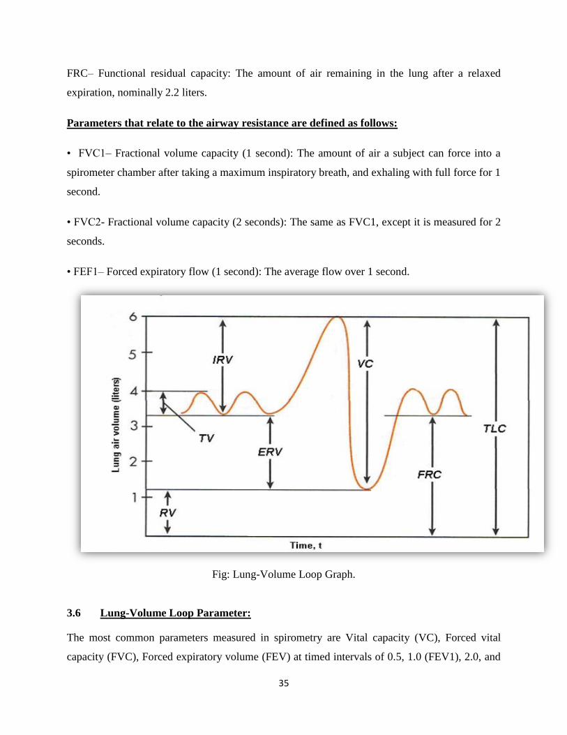
FRC– Functional residual capacity: The amount of air remaining in the lung after a relaxed

expiration, nominally 2.2 liters.

Parameters that relate to the airway resistance are defined as follows:

• FVC1– Fractional volume capacity (1 second): The amount of air a subject can force into a

spirometer chamber after taking a maximum inspiratory breath, and exhaling with full force for 1

second.

• FVC2- Fractional volume capacity (2 seconds): The same as FVC1, except it is measured for 2

seconds.

• FEF1– Forced expiratory flow (1 second): The average flow over 1 second.

Fig: Lung-Volume Loop Graph.

3.6 Lung-Volume Loop Parameter:

The most common parameters measured in spirometry are Vital capacity (VC), Forced vital

capacity (FVC), Forced expiratory volume (FEV) at timed intervals of 0.5, 1.0 (FEV1), 2.0, and

36

3.0 seconds, forced expiratory flow 25–75% (FEF 25–75) and maximal voluntary ventilation

(MVV),[5]

also known as Maximum breathing capacity.[6]

Other tests may be performed in certain

situations.

Results are usually given in both raw data (liters, liters per second) and percent predicted—the

test result as a percent of the "predicted values" for the patients of similar characteristics (height,

age, sex, and sometimes race and weight). The interpretation of the results can vary depending

on the physician and the source of the predicted values. Generally speaking, results nearest to

100% predicted are the most normal, and results over 80% are often considered normal. Multiple

publications of predicted values have been published and may be calculated online based on age,

sex, weight, and ethnicity. However, review by a doctor is necessary for accurate diagnosis of

any individual situation. A bronchodilator is also given in certain circumstances and a pre/post

graph comparison is done to assess the effectiveness of the bronchodilator. See the example

printout. Functional (FRC) cannot be measured via spirometry, but it can be measured with

a plethysmo- graph or dilution tests (for example, helium dilution test).

Fig: Flow-Volume Loop Graph.

37

3.7 Flow-Volume Loop Graph Parameter:

FORCED EXPIRATORY VOLUME AT (t) SECONDS (FEVt)

The forced expiratory volume at (t) seconds is the volume of air expired during a given time

interval (t) from the beginning of the forced vital capacity maneuver. The FEVt can be at 0.5, 3,

or 6 seconds, but the FEV at 1 second is the most widely used standardized parameter in lung

function. The FEV1, just like the FVC, can be reduced in both obstructive and restrictive airway

diseases. A distinction between these two patterns of dysfunction can be inferred by relating the

FEVt to the vital capacity and expressing it as a ratio FEVt/VC.

RATIO OF EXPIRED VOLUME TO FLOW (FEV1/FVC) and (FEV1/FEV6)

The FEV1/FVC ratio is the standard index for assessing and quantifying airflow limitation.

However, this ratio naturally declines with age in adults due in part to loss of elastic recoil of the

lungs. The FEV1/FEV6 ratio is relating how much volume is expired in the first second of a

forced vital capacity maneuver to that expired after six seconds.

3.8 FORCED AVERAGE EXPIRATORY FLOWAS A PERCENTAGE OF FVC

(FEF 25-75%)

The forced expiratory flow (Fix-y) is the average flow rate during a given volume of the FVC

maneuver. X-Refers to the portion of the FVC for which this average flow is measured. FEF x-y

is expressed as a percentage of the FVC. The portion of 25% to 75% of the capacity expired is

called the maximal mid expiratory flow rate or the forced expiratory flow from 25% to 75% of

the exhaled volume. (MMEFR or FEF 25-75%). This measurement encompasses flow from both

the medium sized and the small airways, and may be a more sensitive indicator for airways

obstruction in patients with normal FEV1and FEV1/FVC values.

38

1. PEAK EXPIRATORY FLOW (PEF)

A peak expiratory flow (PEF) is a measure of the initial burst of air leaving the lungs and during

testing can be a good indicator of patient effort. It reflects the portion of air leaving the large

airways.

2. FORCED EXPIRATORY TIME (FET)

The time taken to forcefully exhale a volume of air from a position of full inhalation to one of

full exhalation.

Respiration is the process by which gas is exchanged across cell membranes in all living

systems. At the cellular level, oxygen enters the cell and carbon dioxide is excreted. This process

occurs even in dormant systems such as seeds. In human beings, the lung transfers O2from the

ambient air to the blood and exhaust CO2into the atmosphere. The blood in turn carries O2to and

CO2from the cells. In this process, contraction of respiratory muscles such as the diaphragm and

intercostals muscles between the ribs expands the thorax, creating a negative pressure in the

lung, and drawing in oxygen-rich air. The alveoli exchange O2for CO2in the blood flowing into

the lung. The output blood then stimulates CO2-sensittive cells called CO2receptors in the

arteries near the carotid sinus. These cells, along with stretch receptors in the respiratory

Sr. No. Diagnosis

Forced Expiration Forced Vital

Capacity

FEV1/FVC

Volume for one

second

FVC (Liters)

FEV1 (Liters)

1 Normal Person Normal Normal Normal

2 Airway Obstruction Low Normal / Low Low

3 Airway Restriction Normal Low Low

4 Combination of Low Low Low

Obstruction / Restriction

39

muscles, send out nerve impulses to the medulla oblongata region of the brain stem. The output

from the brain stem is fed back to the respiratory muscles. This controls the breathing rate.

Measurements of blood partial pressure of CO2called PCO2, or partial pressure of O2, called

PO2, show that the respiration rate is controlled by these factors. An increase in PCO2increases

the breathing rate, as illustrated in Figure 1. CO2is a waste product of respiration that must be

swept away as it builds up in the lung. On the other hand, as pO2increases, the breathing rate

slows down, as indicated in the figure. In this case, the demand for oxygen-rich fresh air

decreases. In order to diagnose diseases of the lung such as emphysema or bronchitis, clinicians

need to measure air volumes and flow rates. The nominal volumes, illustrated in Figure 2, are

measured by spirometers and plethysmograph, such as are described further on this paper.

Commonly measured volumes are defined as follow:

• TV– Tidal volume: The volume of air exchanged in relaxed breathing, nominally 0.6 liters.

• IRV– Inspiratory reserve volume: The additional air one can inhale with maximum inspiratory

effort above a relaxed inspiration, nominally 3 liters.

• ERV– Expiratory reserve volume: The additional air one can exhale with maximum effort

beyond a relaxed expiration, nominally 1.2 liters.

• VC– Vital capacity: The total volume of air one can exchange with maximum effort, nominally

5 liters.

• RV– Residual volume: The air that remains in a normal lung after full expiratory effort,

nominally 1 liter.

• FRC– Functional residual capacity: The amount of air remaining in the lung after a relaxed

expiration, nominally 2.2 liters. Parameters that relate to the airway resistance are defined as

follows:

• FVC1– Fractional volume capacity (1 second): The amount of air a subject can force into a

spirometer chamber after taking a maximum inspiratory breath, and exhaling with full force for 1

second.

40

• FVC2- Fractional volume capacity (2 seconds): The same as FVC1, except it is measured for 2

seconds.

• FEF1– Forced expiratory flow (1 second): The average flow over 1 second.

To evaluate the efficiency and the possible detection of respiratory disorders is needed clinical

testing in order to know the patient's condition. Ventilator Functional Test (VFT) is a practice

that allows:

• Measuring lung capacity or, alternatively, the patient's respiratory impairment

• Diagnose different types of respiratory illnesses

• Assess the patient's response to specific therapies and disorders

• Preoperative diagnosis to determine if the presence of a respiratory illness increases the risk of

surgery

The VFT techniques that commonly are used are Spirometry and Plethysmograph.

A trained respiratory nurse performed spirometry using a portable Micro lab 3300 spirometer.

Three forced expiratory maneuvers which met the ATS standards for acceptability (225) were

obtained where possible and repeated 15 minutes after the administration of salbutamol, 400mcg

via a spacer. Results were classified into four groups based on post-bronchodilator values (unless

the patient had only performed pre-bronchodilator testing):

1. COPD: FEV1/FVC ratio <0.7. Severity was based on the GOLD classification (10) using

FEV % predicted: mild =80%, moderate 50-79%, severe 30-49%, and very severe <30%

2. Asthma: post-bronchodilator increase in FEV1 > 200ml and =12% and post bronchodilator

FEV1/FVC =0.7.

3. Small airways disease (SAD): mid-expiratory flow (MEF25-75%) <55% predicted and flow-

volume curve configuration convex to volume axis on downward limb (in the presence of normal

FEV1, FVC and FEV1/FVC ratio).

41

4. Restrictive or mixed obstructive-restrictive pattern: FVC <80% predicted, FEV1/FVC ratio

=0.7.

3.9 Forced Vital Capacity (FVC):

When the A to D data were converted to volume data, differences were found between the

calculated and published (Hankinson 1982) values. The FVC was the largest volume in each

waveform data file. Differences in FVC values resulted when the waveform data did not start

with a zero A to D value. Those waveforms with initial nonzero A to D values were corrected by

subtracting the A to D offset from all subsequent values in those data files. Even after the

changes were made to correct for the offset, differences were still noticed in the FVC of several

waveforms. Waveform 17 had the largest difference, 17 ml (0.29%), in FVC. The remainder of

the waveforms was within 7 ml of the published value, although the published values were only

reported to the nearest 10 ml. Table 1 shows the published values and the values calculated from

the waveform data files and Table 2 shows the differences between the two values. (FEF max l

the published FEF for each waveform was the largest max flow observed using the parabolic

fitted waveform data. There is no definitive literature supporting a specific method of

determining FEF. The time interval for which max the flow must be maintained varies among

different authors. Cotes (1965) states flow must be maintained for 10 ms, Smith and Gaensler

(1975) use a duration of 100 ms, and others state simply that FEF occurs during the "steepest

max ration" of the volume-time curve (Morgan 1975; Morris 1984). The FEF calculated from the

data files by max differentiating the volume every 10 ms always exceeded the published value, in

some cases by as much as 16% (Table 2). These large differences between calculation techniques

create uncertainty about the "true" value for FEFmax.

Forced Expiratory Volume in One Second (FEV11 the FEV1 is the volume exhaled in one

second, starting from the time zero point determined by back-extrapolating from the FEFmax to

the zero volume intercept (Morris 1984). The variability in the FEFmax caused by the

calculation technique resulted in a corresponding variability in the FEV1 because time zero was

changed (Smith 1975). The problem is best illustrated by waveform (Appendix A), which had a

high initial flow that slowed abruptly and then resumed. The highest instantaneous flow (4.84 lis)

occurred during the initial portion of the expiration, and again during the second portion. If the

42

first peak was used, the FEV1 was 2.40 1. If the second peak was used the FEV1 was 2.52 1, for

an apparent error of 120 ml or 4.8%.

3.10 Maximum Mid-expiratory Flow (FEF25-75%):

The published FEF25-75% values were measured from the filtered waveform data, using the

average flow during the exhalation of the middle 50% of the FVC. The FEF25-75% calculated

from the unfiltered data files was consistently higher than the published values using filtered data

Calculating the FEF25-75% from the digitized data revealed a potential problem. If a data point

was not sampled at exactly the volume of FEV25% or the FEV75% during the spirogram,

differences were introduced by using either the preceding or following sampled points.

Interpolating between these points is required to obtain the correct volume at FEV25% or

FEV75%’ Waveform 15 was used to illustrate the problem. Table 3 lists the results obtained

when the preceding, interpolated, and following data points for FEV25% and FEV75% were

used. Effect of using the different data points to calculate FEF25-75%’ the FEF25-75% using the

interpolated points is 4% greater than the published value for waveform. Similar differences

from the published values were found in all waveforms.

3.11 Quality of the spirometry:

A spirometric test is effort –dependent and needs adequate coordination between the technician,

the patient, and the equipment. The patients have to inhale completely before exhaling all the air,

and at least for 6 seconds. People tend to get exhausted if they do it correctly. The technician has

to motivate the participants to perform this as best as possible t 3-6 times consecutive in a

positive and supportive manner. The spirometric tests from Troms 5 were carried out with the

use of one spirometer only, a “Sensor medics Vmax 20.” The American Thoracic Society-criteria

for spirometry testing were adopted. Calibration of the instrument was performed every morning

and at the machines request. Three trained technicians shared the conducting of the spirometry.

The subjects were sitting, using a nose clip, and were instructed to blow as long as possible, for

at least six seconds. The participants took a full inspiration before inserting the mouthpiece

(“open circuit”). At least three exhalations where required. We had one spirometer and three

trained technicians performing 4102 spirometry tests. The 74 subjects, who blew for more than

three, but less than six seconds, were included in the analyses. Excluding these subjects induced

43

only minimal and insignificant changes of the results. Many other studies consist of smaller

surveys from different parts of a country or from different countries, using different spirometers

and more than three technicians. The validity of the test is strengthened in Troms 5 methodology.

3.12 Quality test:

1. Reversibility tests:

According to GOLD guidelines the diagnosis of COPD should be based on post-bronchdilatator

spirometry. Spirometry was only a small part of the survey, and reversibility tests were not done

due to the work-load of the whole survey. The omission of reversibility testing is a weakness of

our study and made it impossible to describe the prevalence of COPD according to GOLD

guidelines. Johannessen et al (61) found that the prevalence of FEV1/FVC below 70% decreased

by approximately 18% after inhalation of a beta2-agonist for subjects 60 years old and above.

Our spirometric values would probably have been somewhat higher if they had been based on

post-bronchdilatator spirometry. However, the frequency in our study of FEV1/FVC ratio less

than 70 % among subject 75-79 years was similar to the frequencies found by Lund back et al

(60) after reversibility testing in subjects aged 76-77 years, both in smokers and never smokers.

The negative effect of not doing reversibility testing may to some degree have been reduced by

the fact that on-going medication, including anti-asthma medicines, had not been interrupted. In

later Troms studies I would encourage those who plan for the spirometry to do reversibility tests.

2. Age and diagnostic criteria:

The discussion of the criteria of COPD, whether to use FEV1/FVC <70% of FEV1/FV6 or LLN

of FEV1 is an ongoing discussion (19; 23; 57; 118; 119) which has lasted since GOLD published

their first program in 2001 (1). There is still no conclusion on the criteria of COPD, and GOLD

has not changed their definition. Many epidemiological surveys (4; 19; 29; 120-122) say the

FEV1/FVC ratio falls significantly after the age of 60. The reduction in lung function can to

some degree be explained by the structural changes that take place in the airways with increasing

age, including dilatation of the alveoli and loss of supportive tissue in the peripheral airways

called “senile emphysema.” Another aspect of normal ageing is loss of muscular tissue generally

and reduced physical endurance. Height-loss during life is normal, and actual height may differ

significant from the reported height. The elderly suffer, in addition, from other diseases, co-

44

morbidities which may influence the lung function (19). Heart failure, in particular, is known to

be associated with reduced spirometric values, including the FEV1/FVC ratio in severe cases.

The elderly part of the population increases year by year, and it is necessary to derive more

equations adapted to the elderly. There is a lack of reference data adjusted for elderly subjects

(124). The existing data are based on relatively small samples, some of them based on self

reported height (22) which may be a bias. Vollmer et al states (119) “Use of the FEV1/FVC

<LLN criterion instead of the FEV1/FVC<0.7 should minimize known age biases and better

reflect clinically significant irreversible airflow limitation”. Our study in paper 1 also supports

the use of the FEV1/FEV6 as a practical substitute for the FEV1/FVC, but we recommend

lowering the threshold in the elderly. A Pub-Med search in January 2012 (COPD AND reference

equations for elderly) found 24 papers of which only two (125;126) had actually derived new

equations, and none of them were derived for elderly only (the fist for 27-82 years of age, the

second for 40-69 years). Because of the normal ageing and reduction in lung function we suggest

to change reference equation adjusted to elderly when performing spirometry on persons 70

years of age and older to FEV1/FVC<0.65. The FEV1/FVC ratio is a practical indicator of the

lung function. It is easily measured, and can be used without the need of reference equations.

The application of the 70% threshold in all ages is an oversimplification, as previously stated by

Enright, Falaschetti, and Hardie (4; 19; 29). Adjustments have to be done to make the measure

clinically useful and credible. Sweden has recently changed their guideline-recommendations in

COPD. For people 65 years of age and older they recommend FEV1/FVC<0.65 (127) which is

partly in agreement with our recommendations in paper 1. I suggest that more research has to be

done to persons 60 years of age and older, and use the threshold FEV1/FVC<0.65 to avoid over

diagnosis.

3. Measurement of ventilator function by spirometry:

Spirometry is a non-invasive test of ventilator lung function used to measure dynamic lung

volumes. The ready availability of spirometry and the ease with which it can be performed using

simple equipment makes it the most important test to detect, quantify, and monitor diseases such

as COPD that limit ventilator capacity. Spirometry is recorded as either a spirogram (a plot of

volume against time) or a flow-volume curve (a plot of volume against flow). The most

commonly measured indices recorded following maximal inspiration and forced expiration are:

45

1. Forced expiratory volume in one second (FEV1)

2. Forced vital capacity (FVC)

3. FEV1/FVC ratio or forced expiratory ratio (FER)

4. Maximal mid-expiratory flow rate (MMEF) or forced expiratory flow over the middle half of

the FVC manoeuvre (FEF25-75%)

5. Peak expiratory flow (PEF)

4 Classification of abnormal spirometry:

Spirometry can be classified on the basis of these major indices into three abnormal patterns.

1. An obstructive ventilator defect with reduced FEV1, FEV1/FVC ratio, or PEF.

2. A restrictive pattern with loss of lung volume without airflow limitation suggested by low

FVC but a normal or high FEV1/FVC ratio.

3. A mixed obstructive and restrictive pattern with airflow limitation and loss of lung volume

shown by low FVC but low FEV1/FVC ratio.

The shape of the flow-volume curve may also vary between an obstructive defect, where the

expiratory curve is convex towards flow and volume axes, and a restrictive disease where the

shape may be concave towards the axes. More complex tests of ventilator function normally

undertaken in a physiology laboratory setting, such as measurement of total lung capacity and

residual volume, are required to confirm both the restrictive and mixed obstructive/restrictive

abnormalities. A particular confounder can exist where a high residual volume due to air-

trapping causes the decrease in FVC giving the false appearance of restriction.

5. Spirometer calibration:

The accuracy of testing is affected by the calibration of the spirometer. Calibration is the

procedure for establishing the relationship between sensor-determined values of flow or volume

and the actual flow or volume. Most spirometers suitable for use in primary care automatically

adjust the accuracy of the spirometer after calibration, though in some cases the adjustment can

46

only be carried out by the distributor or manufacturer. Recommendations updated in 2005 in a

joint report by American Thoracic Society and European Respiratory Society, state that the

calibration of a spirometer should be checked daily with a 3-litre calibration syringe and periodic

testing with a biological control should be carried out to check the stability of the instrument. In

practice, calibration accuracy checks are rarely performed in primary care. Only 22% of

practices surveyed in Australia ever used a calibration syringe and fewer than 2% carried out

daily checks. As stated earlier, the National Lung Health Education Program in the US

recommended developing alternatives to remove the need for this requirement.

6. Spirometer design:

Spirometers meeting recommendations for suitability for use in primary care should be of lower

cost, smaller in size, easier to use, easier to have calibration checks performed and have good

quality assurance features. Further, monitoring quality electronically and displaying specific

messages when errors are detected, assists the operator to obtain high quality spirometry. In

primary care, spirometer reliability and ease of maintenance are considered particularly

important equipment features. The use of ultrasonic technology to measure airflow in a

spirometer designed without moving parts is one way of eliminating inaccuracy due to

instrument errors inherent in some other operating systems. An example is the Easy One™ (ndd

Medizintecknik AG Technoparkstrasse, Switzerland), a handheld spirometer that should in

theory maintain its accuracy throughout its operational life. Influencing spirometry use in clinical

practice despite the development of evidence-based guidelines for clinicians, it is known that

spirometry uptake and implementation remains low in many conditions including COPD

(115,116). A number of reasons may be contributing at levels other than those of practitioner

knowledge and skills, including barriers due to structural, operational, peer-group and

communication difficulties. Such barriers may be addressed through educational interventions,

audit and feedback and reminders (117). An educational intervention in Canada was shown to

increase the appropriate use of spirometry in general practice to 37%, almost doubling the pre-

intervention rate of 20% (118). However under-use and variation in use of spirometry, compared

with guideline specified indications, persisted in a Dutch study of GPs and practice assistants in

practices equipped with spirometers fourteen months after extensive spirometry training (119).

7. Cost effectiveness of spirometry:

47

A cost effectiveness study in the UK, using data from one study in the Netherlands (108)

calculated that the cost per life year gained from using spirometry opportunistically for case

finding was £713.16 and the cost per quality adjusted life year gained was £816.56 (15,86). This

is a good cost effectiveness ratio compared to other screening programmers (120). The cost per

case of COPD or asthma detected in a screening programmed in general practice in the

Netherlands, involving symptom enquiry and lung function measurement, was much lower than

that of screening for hypercholesterolemia, prostate cancer or breast cancer (121).

8. Acceptability of spirometry:

There is little direct information on the acceptability of spirometry to patients. A participation

refusal rate of 34% was found in a prospective European study in general practice to detect

COPD and asthma, although some of the refuses agreed to participate in testing at home (121).

Another practice-based case finding study in Holland had a 2.5% refusal rate but no information

on the reasons for refusal was given (108). A UK study found only 2% of patients aged over 45

years refused opportunistic spirometry screening for COPD when attending for a consultation,

while 20% refused home-based screening and only 33% actually had spirometry at home (110).

Spirometry invitations in this study were not offered to every patient attending the practice

during screening sessions. The acceptability of spirometry may depend on the reason for

performing it. Thus in a practice-based study with the primary objective of investigating

spirometry and smoking cessation, 31% of smokers refused to participate, though their reasons

were not reported (122).

9. Measurement of quality of life

The St. George’s Respiratory Questionnaire (SGRQ) (226) was used to measure health related

quality of life. It was devised to provide a measure of quality of life specifically in airways

disease and be more sensitive than general quality of life measures. The SGRQ has been shown

to be sensitive and repeatable. A difference in total score of about four points indicates a

clinically significant difference between populations (226). An improvement of about four points

also indicates a clinically important therapeutic effect (227). The SGRQ is applicable in a range

of disease severity (228). There are seventy-six items, relating to frequency and severity of

respiratory symptoms, activities that cause or are limited by breathlessness, impacts on social

48

functioning or psychological disturbance resulting from respiratory disease. Participants

completed the questionnaire during the clinical assessment and without assistance. It was

checked for completeness by the researcher. The total score and subscale scores for symptoms,

activity, and impacts were calculated.

10. Diagnosis of respiratory disease

A diagnosis of COPD, emphysema or COAD was recorded for 36 (85%) participants who

completed the clinical assessment. These terms were used with varying frequency in practice

records. They were used interchangeably as diagnostic terms until guidelines introduced specific

definitions for COPD from around 1995. The results included here use the term COPD,

irrespective of which term was used in practice records. Additional diagnoses were also recorded

in participants with COPD, asthma in 18 (50%) participants and chronic bronchitis in 13 (36%)

participants.

11. Participants with no recorded diagnosis of COPD:

Six participants who completed clinical assessments did not actually have a diagnosis of COPD

(or equivalent) recorded in the practice records, although GPs had been asked to select

participants who met this inclusion criterion. Four participants who had smoked for many years

(mean 51 pack years) did have COPD according to study spirometry. In one case, the practice

record covered only the previous three years and no respiratory diagnosis was recorded. This

participant called the breathing problem “emphysema” and was using a short-acting beta-2

agonist occasionally. Spirometry showed COPD was classified as severe (FEV1 45% predicted).

Two participants who were current smokers, had frequent diagnoses of respiratory tract

infections recorded (but no diagnosis of chronic bronchitis), despite reporting symptoms of

cough, breathlessness and phlegm (in winter and on most days for as long as three months each

year) on the study questionnaire. Asthma was the principal respiratory diagnosis recorded for one

participant (ex-smoker, aged 77 years). The participant called it a “breathing problem” and

reported breathlessness walking on level ground (MRC grade 3) and cough for at least three

months in the winter. Two other participants had a diagnosis of asthma recorded and their study

spirometry did not show fixed airflow limitation.

49

12. Spirometry results:

Patients with a diagnosis of COPD Spirometry results were consistent with a diagnosis of COPD

(FEV1/FVC <0.7) in 30 (83%) of the 36 participants with doctor-recorded COPD. COPD

classification of severity based on FEV1 % predicted using GOLD criteria was moderate for 16

(53%) participants, severe for 8 (27%) participants and very severe for 6 (20%) participants. Of

six participants whose spirometry did not meet the criterion for airflow obstruction in COPD,

five participants had restrictive or mixed obstructive-restrictive pattern on spirometry. One of

these had recorded diagnoses of both COPD and Idiopathic Pulmonary Fibrosis. There was a

record of spirometry at diagnosis and within two years for these participants. One participant was

classified with small airways disease on spirometry.

50

Chapter 4

4.1 Principles of Operation (Spirometer):

DEVELOPMENT:

Respiratory function we can consider as a physical event in two stages, inhalation (fresh air to

the lungs) and exhalation (hot air out the lungs). Generally, when a doctor wants to establish

whether or not a patient has a respiratory illness, need to know certain parameters, such as the

pressure difference between the environment and the lung, and thanks to this pressure difference,

the lung can make the exchange of gases, the flow of exchange during the respiratory process,

and the volume of air entering and leaving the lungs. To measure these parameters during the

exhalation process, we designed a Flow Spirometer, which is an instrument that measures the

instantaneous change in volume and flow of air entering the lungs during ventilation, across the

trace and/or a register of volume-time and flow-volume of respiration. Flow spirometers

obtained directly ventilator flow and air volume is obtained by electronic integration of flow.

The block diagram of the architecture of a spirometer flow. It consists of four stages divided as

follows: sensing stage, signal conditioning stage, voltage integration stage and signal processing.

51

Fig: Block Diagram of Spirometer

FIGURE: Implementation of Spirometer

Fig: Analog Front End Design

Sensing Stage:

The sensing stage is formed by a flow transducer type Pneumo-tacograph and differential

pressure sensor. Depending on the mechanical principle used, different Pneumo-tacograph types,

such as turbine or thermal gradient, but the most widely used, for its practicality and low cost are

the differential pressure Pneumo-tacograph. In the differential pressure Pneumo-tacograph,

exhaled gas passes through a mesh whose resistance generates a pressure difference that is

proportional to the flow (F) of gas passing through it.

This pressure difference is measured by a differential pressure sensor type MPX5050DP, which

generates an electrical signal output from which the assets of flow. This sensor is a "strain

52

gauge," and its output a voltage signal, that is proportional to the differential pressure between its

inlets, according to the following expression

4.2 PRESSURE SENSOR:

Differential pressure sensor:

This sensor measures the difference between two pressures, one connected to each side of the

sensor. Differential pressure sensors are used to measure many properties, such as pressure drops

across oil filters or air filters, fluid levels (by comparing the pressure above and below the liquid)

or flow rates (by measuring the change in pressure across a restriction). Technically speaking,

most pressure sensors are really differential pressure sensors; for example a gauge pressure

sensor is merely a differential pressure sensor in which one side is open to the ambient

atmosphere.

Piezoresistivity strain gauge:

Uses the Piezoresistivity effect of bonded or formed strain gauges to detect strain due to applied

pressure. Common technology types are Silicon (Monocrystalline), Polysilicon Thin Film,

Bonded Metal Foil, Thick Film, and Sputtered Thin Film. Generally, the strain gauges are

connected to form a Wheatstone bridge circuit to maximize the output of the sensor and to

reduce sensitivity to errors. This is the most commonly employed sensing technology for general

purpose pressure measurement. Generally, these technologies are suited to measure absolute,

gauge, vacuum, and differential pressures.

Normal Values of Pulmonary Function Tests

PULMONARY FUNCTION TEST NORMAL VALUE (95 PERCENT CONFIDENCE

INTERVAL)

FEV1 80% to 120%

FVC 80% to 120%

Absolute FEV1 /FVC ratio Within 5% of the predicted ratio

TLC 80% to 120%

53

FRC 75% to 120%

RV 75% to 120%

Sensor Transfer characters (MPX5050DP):

CALCULATION’S:

TRANSFER FUNCTION = VOUT=VS*(0.018*P+0.04)

Pressure P=Vout/1.45

Calculation of volume: PV=NRT, V=NRT/P T=Temp N=1

54

Fig: Sensor MPX5050DP

Fig: Design of Mouth Piece (Dimensional)

Signal Conditioning Stage:

Because the pressure differences are very low and hence the output voltage is very small, we

need a signal conditioning stage in which it uses a type instrumentation amplifier whose main

features are to have high input impedance and a high rejection of common signs, and a low-pass

filter Butterworth 2nd order with a cutoff frequency of 15 Hz.

55

Fig: Differential Pressure sensor with Signal Amplification

Fig: Analog Front End of Spirometer

56

Fig: ADC in FPGA Module & FTDI Module Interface with pc (USB)

Fig: Output waveform calculation

57

4.4 Processing Stage:

The instrument has a data acquisition system for display on CRO or transfer to a computer. This

system is based on FPGA (ADC) microcontroller, which has an 8-bits analog to digital

converter. The system receives the signal from the spirometer through a buffer to avoid applying

it directly to the analog-digital converter of the microcontroller. The microcontroller is

responsible for generating the base time of sampling frequency. The advantage of using a

microcontroller like data acquisition system is its low cost, since the microcontroller. In addition,

you can easily adapt to any computer including laptops. Furthermore, any changes to the

programming of the microcontroller can be done without being removed from the card, because

the microcontroller has the verilog programming option ('In System Programming'). To begin the

processing of data in the microprocessor, the integer variables, the floating point constant values,

and the resolution which will be the conversion are defined. Then, to convert A / D, are defined

as input ports and channels where it will convert. The deployment of data is sent to the display

screen of the flow and volume values obtained after digital A / D conversion thereof. If required

to perform another measurement, the integrator is reset (the switch is closed discharging

capacitor, to return it to original condition) to repeat the process.

Signal Conditioning Stage

Because the pressure differences are very low and hence the output voltage is very small, we

need a signal conditioning stage in which it uses a type AD620 instrumentation amplifier whose

main features are to have a high input impedance and a high rejection of common signs, and a

low-pass filter Butterworth 2nd order with a cutoff frequency of 5 Hz. The figure 6, show the

schematic diagram of this stage.

Sensing Stage

The sensing stage is formed by a flow transducer type Pneumo-tacograph and differential

pressure sensor. Depending on the mechanical principle used, different Pneumo-tacograph types,

such as turbine or thermal gradient, but the most widely used, for its practicality and low cost are

the differential pressure Pneumo-tacograph. In the differential pressure Pneumo-tacograph,

exhaled gas passes through a mesh whose resistance generates a pressure difference that is

proportional to the flow (F) of gas passing through it.

58

Chapter 5

5.1 Introduction Sensor Design

Sensors are devices that detect or measure physical and chemical quantities such as temperature,

pressure, sound, and concentration. The measured are converted into an electrical signal. The

main requirements of a good sensor are high sensitivity, fast response, low cost, high volume

production, and high reliability. Sensors continue to make Author to whom correspondence

should be addressed. Significant impact in everyday life with applications ranging from

biomedical to automotive industry. This has led to intensive research activities across the world

in developing new sensing materials and technologies. With the advent of nanotechnology,

research is underway to create miniaturized sensors. Miniaturized sensors can lead to reduced

weight, lower power consumption, and low cost. Materials such as inorganic semiconductors are

used in making nanosensors.

A pressure sensor measures pressure, typically of gases or liquids. Pressure is an expression of

the force required to stop a fluid from expanding, and is usually stated in terms of force per unit

area. A pressure sensor usually acts as a transducer; it generates a signal as a function of the

pressure imposed. For the purposes of this article, such a signal is electrical. Pressure sensors are

used for control and monitoring in thousands of everyday applications. Pressure sensors can also

be used to indirectly measure other variables such as fluid/gas flow, speed, water level, and

altitude. Pressure sensors can alternatively be called pressure transducers, pressure transmitters,

pressure senders, pressure indicators, piezometers and manometers, among other names. Pressure

sensors can vary drastically in technology, design, performance, application suitability, and cost.

A conservative estimate would be that there may be over 50 technologies and at least 300

companies making pressure sensors worldwide. There is also a category of pressure sensors that

are designed to measure in a dynamic mode for capturing very high speed changes in pressure.

Example applications for this type of sensor would be in the measuring of combustion pressure

in an engine cylinder or in a gas turbine. These sensors are commonly manufactured out of

piezoelectric materials such as quartz.

Some pressure sensors, such as those found in some traffic enforcement cameras, function in a

binary (off/on) manner, i.e., when pressure is applied to a pressure sensor, the sensor acts to

59

complete or break an electrical circuit. These types of sensors are also known as a pressure

switch.

5.2 Types of pressure measurements:

a) Silicon piezoresistive pressure sensors

Pressure sensors can be classified in terms of pressure ranges they measure, temperature ranges

of operation, and most importantly the type of pressure they measure. Pressure sensors are

variously named according to their purpose, but the same technology may be used under

different names.

b) Absolute pressure sensor:

This sensor measures the pressure relative to perfect vacuum.

c) Gauge pressure sensor

This sensor measures the pressure relative to atmospheric pressure. A tire pressure gauge is an

example of gauge pressure measurement; when it indicates zero, then the pressure it is measuring

is the same as the ambient pressure.

d) Vacuum pressure sensor

This term can cause confusion. It may be used to describe a sensor that measures pressures

below atmospheric pressure, showing the difference between that low pressure and atmospheric

pressure (i.e. negative gauge pressure), but it may also be used to describe a sensor that measures

low pressure relative to perfect vacuum (i.e. absolute pressure).

e) Differential pressure sensor

This sensor measures the difference between two pressures, one connected to each side of the

sensor. Differential pressure sensors are used to measure many properties, such as pressure drops

across oil filters or air filters, fluid levels (by comparing the pressure above and below the liquid)

or flow rates (by measuring the change in pressure across a restriction). Technically speaking,

most pressure sensors are really differential pressure sensors; for example a gauge pressure

60

sensor is merely a differential pressure sensor in which one side is open to the ambient

atmosphere.

f) Sealed pressure sensor

This sensor is similar to a gauge pressure sensor except that it measures pressure relative to some

fixed pressure rather than the ambient atmospheric pressure (which varies according to the

location and the weather).

5.3 Pressure-sensing technology

There are two basic categories of analog pressure sensors,

Force collector types these types of electronic pressure sensors generally use a force collector

(such a diaphragm, piston, bourdon tube, or bellows) to measure strain (or deflection) due to

applied force (pressure) over an area.

1) Piezoresistive strain gauge

Uses the piezoresistive effect of bonded or formed strain gauges to detect strain due to applied

pressure. Common technology types are Silicon (Monocrystalline), Polysilicon Thin Film,

Bonded Metal Foil, Thick Film, and Sputtered Thin Film. Generally, the strain gauges are

connected to form a Wheatstone bridge circuit to maximize the output of the sensor and to

reduce sensitivity to errors. This is the most commonly employed sensing technology for general

purpose pressure measurement. Generally, these technologies are suited to measure absolute,

gauge, vacuum, and differential pressures.

2) Capacitive

Uses a diaphragm and pressure cavity to create a variable capacitor to detect strain due to applied

pressure. Common technologies use metal, ceramic, and silicon diaphragms. Generally, these

technologies are most applied to low pressures (Absolute, Differential, and Gauge)

3) Electromagnetic

Measures the displacement of a diaphragm by means of changes in inductance (reluctance),

LVDT, Hall Effect, or by eddy current principle.

61

4) Piezoelectric

Uses the piezoelectric effect in certain materials such as quartz to measure the strain upon the

sensing mechanism due to pressure. This technology is commonly employed for the

measurement of highly dynamic pressures.

5) Optical

Techniques include the use of the physical change of an optical fiber to detect strain due to

applied pressure. A common example of this type utilizes Fiber Bragg Gratings. This technology

is employed in challenging applications where the measurement may be highly remote, under

high temperature, or may benefit from technologies inherently immune to electromagnetic

interference. Another analogous technique utilizes an elastic film constructed in layers that can

change reflected wavelengths according to the applied pressure (strain).[1]

6) Potentiometric

Uses the motion of a wiper along a resistive mechanism to detect the strain caused by applied

pressure.

Other types:

These types of electronic pressure sensors use other properties (such as density) to infer pressure

of a gas, or liquid.

7) Resonant

Uses the changes in resonant frequency in a sensing mechanism to measure stress, or changes in

gas density, caused by applied pressure. This technology may be used in conjunction with a force

collector, such as those in the category above. Alternatively, resonant technology may be

employed by exposing the resonating element itself to the media, whereby the resonant

frequency is dependent upon the density of the media. Sensors have been made out of vibrating

wire, vibrating cylinders, quartz, and silicon MEMS. Generally, this technology is considered to

provide very stable readings over time.

62

8) Thermal

Uses the changes in thermal conductivity of a gas due to density changes to measure pressure. A

common example of this type is the Pirani gauge.

9) Ionization

Measures the flow of charged gas particles (ions) which varies due to density changes to measure

pressure. Common examples are the Hot and Cold Cathode gauges.

5.4 Applications:

There are many applications for pressure sensors:

1) Pressure sensing

This is where the measurement of interest is pressure, expressed as a force per unit area. This is

useful in weather instrumentation, aircraft, automobiles, and any other machinery that has

pressure functionality implemented.

2) Altitude sensing

This is useful in aircraft, rockets, satellites, weather balloons, and many other applications. All

these applications make use of the relationship between changes in pressure relative to the

altitude. Barometric pressure sensors can have an altitude resolution of less than 1 meter, which

is significantly better than GPS systems (about 20 meters altitude resolution). In navigation

applications altimeters are used to distinguish between stacked road levels for car navigation and

floor levels in buildings for pedestrian navigation.

3) Flow sensing

This is the use of pressure sensors in conjunction with the venture effect to measure flow.

Differential pressure is measured between two segments of a venture tube that have a different

aperture. The pressure difference between the two segments is directly proportional to the flow

rate through the venture tube. A low pressure sensor is almost always required as the pressure

difference is relatively small.

63

4) Level / depth sensing

A pressure sensor may also be used to calculate the level of a fluid. This technique is commonly

employed to measure the depth of a submerged body (such as a diver or submarine), or level of

contents in a tank (such as in a water tower). For most practical purposes, fluid level is directly

proportional to pressure.

5) Leak testing

A pressure sensor may be used to sense the decay of pressure due to a system leak. This is

commonly done by either comparison to a known leak using differential pressure, or by means of

utilizing the pressure sensor to measure pressure change over time.

6) Radiometric Correction of Transducer Output

Piezoresistive transducers configured as Wheatstone bridges often exhibit radiometric behavior

with respect not only to the measured pressure, but also the transducer supply voltage.

64

Chapter 6

6.1 Introduction:

Piezoresistive pressure sensors were some of the first MEMS devices to be commercialized.

Compared to capacitive pressure sensors, they are simpler to integrate with electronics, their

response is more linear, and they are inherently shielded from RF noise. They do, however,

usually require more power during operation, and the fundamental noise limits of the sensor are

higher than their capacitive counterparts. Historically, piezoresistive devices have been dominant

in the pressure sensor market.

6.2 Model Definition:

The model consists square membrane with side 1 mm and thickness 20 μm, supported around its

edges by region 0.1mm wide, which is intended to represent the remainder of the wafer. The

supporting region is fixed on its underside (representing a connection to the thicker handle of the

device die). Near to one edge of the membrane an X-shaped piezoresistor (or Xducer™)1 and

part of its associated interconnects are visible. The piezoresistor is assumed to have a uniform p-

type dopant density of 1.32×1019 cm−3 and a thickness of 400 nm. The interconnects are

assumed to have the same thickness but a dopant density of 1.45×1020 cm−3. Only a part of the

interconnects is included in the geometry, since their conductivity is sufficiently high that they

do not contribute to the voltage output of the device (in practice the interconnects would also be

thicker in addition to having a higher conductivity but this will also have little effect on the

solution). The edges of the die are aligned with the 110 directions of the silicon. The die edges

are also aligned with the global X and Y axes in the COMSOL model. The piezoresistor is

oriented at 45 to the die edge, and so lies in the [100] direction of the crystal. In the COMSOL

model, a coordinate system rotated 45 about the global Z-axis is added to define the orientation

of the crystal.

6.3 DEVICE PHYSICS AND EQUATIONS:

The conductivity of the Xducer™ sensor changes when the membrane in its vicinity is subject to

an applied stress. This effect is known as the piezoresistance effect and is usually associated with

semiconducting materials. In semiconductors, piezoresistance results from the strain-induced

65

alteration of the material’s band structure, and the associated changes in carrier mobility and

number density. The relation between the electric field, E, and the current, J, within a

piezoresistor is:

(1) Where ρ is the resistivity and Δρ is the induced change in the resistivity. In the general

case both ρ and Δρ are rank 2 tensors (matrices). The change in resistance is related to the

stress, σ, by the constitutive relationship:

(2) Where Π is the piezoresistance tensor (SI units: Pa−1Ωm), a material property. Note that

COMSOL’s definition of Π includes the resistivity in each element of the tensor, rather

than having a scalar multiple outside of Π (which is possible only for materials with

isotropic conductivity). Π is in this case a rank-4 tensor; however, it can be represented as

a matrix if the resistivity and stress are converted to vectors within a reduced subscript

notation.

Discussion:

The displacement of the diaphragm as a result of a 100 kPa pressure difference. At the center of

the diaphragm the displacement is 1.2 μm. A simple isotropic model for the deform displacement

given in Ref. 1 predicts an order of magnitude value of 4 μm (assuming a Young’s modulus of

170 GPa and a Poisson’s ratio of 0.06). The agreement is reasonable considering the limitations

of the analytic model, which is derived by a crude variational guess. A more accurate value for

the shear stress in local coordinates at the midpoint of the diaphragm edge is given in Ref. 1 as:

where P is the applied pressure, L is the length of the diaphragm edge, and H is the diaphragm

thickness. This equation predicts the magnitude of the local shear stress to be 35 MPa, in good

agreement with the minimum value shown in Figure 3, which is also 35 MPa. Theoretically the

shear stress should be maximal at the midpoint of the edge of the diaphragm. Figure 4 shows the

shear stress along the edge in the model. This shows a maximum magnitude at the center of each

of the two edges along which the plot is made, but the value of this maximum is less than the

maximum stress in the model, in part due to the boundary conditions employed on the three

dimensional diaphragm. The model: piezoresistive_pressure_sensor_shell.mph shows better

agreement with the theoretical maximum shear stress along this edge. Pressure sensors in their

primitive form existed as strain gauges for over several decades. The miniaturization of pressure

sensors and other mechanical sensors gained considerable attention soon after the invention of

piezoresistivity in silicon and germanium [Smith, 1954]. This activity gained further momentum

66

with the recognition of the excellent mechanical properties of silicon [Peterson, 1982]. The

advent of the micromachining of silicon to carve out mechanical microstructures in silicon and

the already existing expertise in manufacturing microelectronic devices and integrated circuits in

silicon, opened the doors of the highly interdisciplinary area of MEMS and microsystems.

During the past two decades, several industries and academic institutions all over the globe have

been involved in the development and commercialization of micro sensors for industrial,

automobile, defense, space, and biomedical applications. Among the various devices, pressure

sensors using MEMS technology have received great attention because the pressure sensors find

applications in everyday life involving sensing, monitoring, and controlling pressure, and they

therefore constitute 60 to 70 percent of the market amongst the various MEMS devices. As the

requirements widen, new challenges emerge because the pressures range from a few Pascal (Pa)

to several Mega Pascal (MPa) depending on the application and the environment, which vary

from being very sensitive in biomedical applications to being very harsh in industrial and

automobile applications. Hence, they need to be biocompatible in some applications while they

need to be rugged and capable of performing reliably in temperatures well in excess of 80°C to

100°C.They also need to survive in corrosive fluids like ocean water in applications such as

Oceanography. In several applications, such as mapping the pressure on the aero foil of an

aircraft, the package needs to be flat and the device height needs to be restricted to below a

millimeter. Similarly, in biomedical applications such as an intra cranial pressure (ICP) sensor,

where the sensor is inserted into the ventricle, the packaged size should not exceed a diameter of

1mm.

6.4 Pressure Sensor Types and Classification:

Pressure sensors are categorized as absolute, gauge and differential pressure sensors based on the

reference pressure with respect to which the measurement is carried out. Particular applications

are as follows.

(a) Absolute Pressure Sensors

Measure the pressure relative to a reference vacuum encapsulated within the sensor as

shown in Figure1. Such devices are used for atmospheric pressure measurement and as

manifold absolute pressure (MAP) sensors for automobile ignition and airflow control

67

systems. Pressure sensors used for cabin pressure control, launch vehicles, and satellites

also belong to this category.

(b) Gauge Pressure sensors

Measure pressure relative to atmospheric pressure. One side of the diaphragm is vented

to atmospheric pressure as shown in Figure 2. Blood pressure (BP), intra-cranial pressure

(ICP), gas cylinder pressure and most of ground-based pressure measurements are gauge

pressure sensors. Vacuum sensors are gauge sensors designed to operate in the negative

pressure region.

(c) Differential Pressure Sensors

Measure accurately the difference ΔP between two pressures P1 and P2 across the

diaphragm (with ΔP << P1 or P2), and hence need two pressure ports as shown in Figure

3. They find applications in airplanes used in warfare. They are also used in high pressure

oxidation systems where it is required to maintain an oxygen pressure ranging from 1 to

10 atmospheres inside a quartz tube during the oxidation of silicon. In this system, the

outside of the quartz tube is maintained at a slightly higher gas pressure of nitrogen, and

the pressure difference is monitored using a differential pressure sensor which ensures

that the quartz tube does not experience a differential pressure greater than its rupture

stress of 1 atmosphere (105 Pascal). The differential pressure sensor is also used in some

applications where it is desirable to detect small differential pressures superimposed on

large static pressures. In almost all types of pressure sensors, the basic sensing element is

the diaphragm, which deflects in response to the pressure. As the deflections in

diaphragm-based sensors are small they cannot be directly measured. This mechanical

deflection or the resulting strain in the diaphragm is converted ultimately into electrical

signals using suitable transduction mechanisms, namely, capacitive, piezoresistive or

piezo-electric techniques, which are usually employed as adjectives for the pressure

sensors as described below:

(i) Strain gauges and Piezoresistive pressure sensors:

In traditional metal diaphragm-based pressure sensors, the most common method has been to

locate metal strain gauges (foil type) on the metal diaphragm, in positions of maximum stress to

maximize the sensitivity. With the invention of piezoresistivity in Silicon, and silicon

68

micromachining for diaphragm realization, boron-doped silicon piezoresistor have replaced the

metal strain gauges. In this approach, much higher sensitivities have been achieved because the

piezo-resistors are embedded Fig. 3 Schematic diagram of Differential Pressure sensors directly

on the silicon diaphragm by implanting or diffusing boron in the selected regions of maximum

stress as shown in Figure 4(a). These resistors are connected in the form of a Whetstone Bridge

which gives an output when the resistors are strained under the action of the pressure sensed by

the diaphragm. It will be seen in subsequent sections that piezoresistive pressure sensors enable

linear operation over a wide range of pressures. They are also simple to fabricate. As a result,

they have captured the major market of pressure sensors encompassing the automobile industry,

defense, space as well as biomedical applications. Other transduction techniques are capacitance

and piezoelectric approaches and they are identified as capacitive pressure sensor and

piezoelectric pressure sensors respectively.

(ii) Capacitive Pressure Sensor:

A schematic diagram of a silicon micro machined sensor of this type is shown in Figure

4(b).This approach uses the diaphragm as one electrode of a parallel plate capacitor structure and

diaphragm displacement causes a change in capacitance with respect to a fixed electrode. The

merits of capacitive pressure sensors are their high sensitivity, which is practically invariant with

temperature. However, in this case, an electronic circuit is required to convert the capacitance

change into an electrical output. An additional disadvantage of this approach is the nonlinear

relationship between the capacitance and displacement and hence a force-balancing and

linearizing electronic circuit is essential to capture a wide range of pressures.

(iii) Piezoelectric pressure sensors:

Silicon does not show a piezoelectric effect. Therefore, a piezoelectric sensing element, such as

Lead Zirconate Titanate (PZT) or Zinc Oxide (ZnO) is placed/deposited on to the silicon

diaphragm as shown in Figure 4(c). The deflection of the diaphragm induces strain in the

piezoelectric material and hence a charge is generated. These sensors are only suitable for

measuring dynamic pressures and are not suitable for static pressure sensing because

piezoelectric materials only respond to changing strains. The major advantage of this approach is

that an external power supply is not required. In another approach, in which pressure sensors are

69

identified as resonant sensors, the vibration frequency of a mechanical beam or a membrane,

which depends on the extent to which it is stretched, is used This is similar to the vibration

frequency of a violin string. The output signal from a resonant sensor is a frequency, which can

easily be transferred into a digital signal and interfaced with computer systems, without having

to use an Analog to Digital converter. In most of the cases, a quartz resonating beam is used

because these sensors are noted for their high stability and high resolution as a frequency signal

is much more robust than an amplitude (e.g. a voltage). The stability is determined only by the

mechanical properties of the resonator material, which is generally very stable. On the flip side,

resonant silicon sensors are not easy to fabricate and hence become expensive. The high costs

may be compensated by innovative simpler mechanical structures and by simpler electronics. In

all the types of pressure sensors, the diaphragm is invariably, if not always, chosen as the sensing

element. The static and dynamic performance characteristics of the diaphragm are of great

importance and provide suitable design guidelines for designing pressure sensors. These aspects

of micro machined diaphragms are discussed in the following section.

6.5 Piezoresistive Transducer Analyses and Design

Among the various types of pressure sensors, piezoresistive pressure sensors and piezoelectric

pressure sensors work on the principle of converting the strain developed on the sensor chip into

change in resistance and voltage respectively. Therefore, the sensitivity of these two types of

pressure sensors is governed by the location of maximum stress regions on the chip when the

diaphragm is subjected to pressure. On the other hand, the performance of capacitive sensors is

judged by the extent of change in the capacitance of a movable electrode with respect to a fixed

reference electrode. Therefore, the operation range and sensitivity of the capacitive sensor is

determined

(i) by the extent to which the electrode can deflect

(ii) the ability to minimize stray capacitances

(iii) capacitance voltage conversion circuits

Due to their simplicity of fabrication and the wide range of pressures, ranging from a few kPa to

several hundreds of kPa over which they can perform with excellent linearity and accuracy,

piezoresistive pressure sensors have received maximum attention and acceptance in automobiles,

airplanes, missiles, and rockets as well as in biomedical applications. Therefore, in this section,

70

we consider the various design criteria and fabrication process steps involved in the development

of piezoresistive pressure sensors. Following the diaphragm design and identification of the

regions of high stress components on the diaphragm, the next important design parameter is the

design of resistors and their dimensions. In the following sections, we first focus on various

parameters such as the gauge factor and piezorestive coefficient and the factors influencing their

magnitudes, and hence, the sensitivity of the piezoresistive pressure sensors

6.6 Sensitivity (S)

The sensitivity of a pressure sensor is defined as at a particular input voltage. The V0 increases

from 70mV to 210 mV linearly as the pressure is increased from 0 to 2.0bar. The sensitivity for

this device this is equal to 70mV /bar when the input voltage V IN =10V The sensitivity is rather

low for this device because the resistors in this case were fabricated using polycrystalline silicon

whose gauge factor is low compared to that of single crystal diffused resistors. Higher

sensitivities and lower noise levels are typically achieved with diffused or ion implanted single

crystal silicon strain gauges

Fig: Sensitivity of the sheet resistance

71

Fig: Piezoresistive pressure sensor Module

Fig: Sensor with Mesh applied

72

Fig :(a)

Fig: (a), (b): When stress applied on it and %of stress applied on it

73

Fig: Percentage of the stress applied in graphical representation.

6.7 Design concept of Pressure sensor:

Modeling Instructions:

MODEL WIZARD

1 Go to the Model Wizard window.

2 Click Next.

3 In the Add physics tree, select Structural Mechanics>Piezoresistivity>Piezoresistivity,

Boundary Currents (pzrb).

4 Click Next.

5 Find the Studies subsection. In the tree, select Preset Studies>Stationary.

6 Click Finish.

74

GEOMETRY 1

1 In the Model Builder window, under Model 1click Geometry 1.

2 In the Geometry settings window, locate the Units section.

3 From the Length unit list, choose µm.

Import 1

1 Right-click Model 1>Geometry 1and choose Import.

2 In the Import settings window, locate the Import section.

3 Click the Browse button.

4 Browse to the model’s Model Library folder and double-click the file

piezoresistive_pressure_sensor.mphbin.

5 Click the Build All button.

DEFINITIONS

Set up selections for the model.

Explicit 1

1 In the Model Builder window, right-click Definitions and choose Selections>Explicit.

2 In the Explicit settings window, locate the Input Entities section.

3 From the Geometric entity level list, choose Boundary.

4 Select Boundary 46 only.

5 Right-click Model 1>Definitions>Explicit 1and choose Rename.

6 Go to the Rename Explicit dialog box and type Piezoresistor in the New name edit field.

7 Click OK.

75

Explicit 2

1 Right-click Definitions and choose Selections>Explicit.

2 In the Explicit settings window, locate the Input Entities section.

3 From the Geometric entity level list, choose Boundary.

4 Select Boundaries 14, 22, 26, 39, 74, 78, 82, and 106 only.

5 Right-click Model 1>Definitions>Explicit 2and choose Rename.

6 Go to the Rename Explicit dialog box and type Connectionism the New name edit field.

7 Click OK.

Box 1

1 Right-click Definitions and choose Selections>Box.

2 In the Box settings window, locate the Geometric Entity Level section.

3 From the Level list, choose Boundary.

4 Locate the Box Limits section. In the x minimum edit field, type -501.

5 In the x maximum edit field, type 501.

6 In the y minimum edit field, type -30.

7 In the y maximum edit field, type 1000.

8 In the z maximum edit field, type -1.

9 Locate the Output Entities section. From the Include entity if list, choose Entity inside box.

10Right-click Model 1>Definitions>Box 1and choose Rename.

11Go to the Rename Box dialog box and type Membrane (Lower Surface)in the New name edit

field.

76

12Click OK.

Membrane (Lower Surface) 1

1 Right-click Model 1>Definitions>Box 1and choose Duplicate.

2 In the Box settings window, locate the Box Limits section.

3 In the z minimum edit field, type -1.

4 In the z maximum edit field, type inf.

5 Right-click Model 1>Definitions>Membrane (Lower Surface) 1and choose Rename.

6 Go to the Rename Box dialog box and type Membrane (Upper Surface)in the New

name edit field.

7 Click OK.

Box 3

1 Right-click Definitions and choose Selections>Box.

2 In the Box settings window, locate the Geometric Entity Level section.

3 From the Level list, choose Boundary.

4 Locate the Box Limits section. In the z maximum edit field, type -1.

5 Locate the Output Entities section. From the Include entity if list, choose Entity inside box.

6 Right-click Model 1>Definitions>Box 3and choose Rename.

7 Go to the Rename Box dialog box and type Lower Surface in the New name edit field.

8 Click OK.

Lower Surface 1

1 Right-click Model 1>Definitions>Box 3and choose Duplicate.

77

2 In the Box settings window, locate the Box Limits section.

3 In the z minimum edit field, type -1.

4 In the z maximum edit field, type inf.

5 Right-click Model 1>Definitions>Lower Surface 1and choose Rename.

6 Go to the Rename Box dialog box and type Upper Surface in the New name edit field.

7 Click OK.

Difference 1

1 Right-click Definitions and choose Selections>Difference.

2 In the Difference settings window, locate the Geometric Entity Level section.

3 From the Level list, choose Boundary.

4 Locate the Input Entities section. Under Selections to add, click Add.

5 Go to the Add dialog box.

6 In the Selections to add list, select Lower Surface.

7 Click the Unbutton.

8 In the Difference settings window, locate the Input Entities section.

9 Under Selections to subtract, click Add.

10Go to the Add dialog box.

11In the Selections to subtract list, select Membrane (Lower Surface).

12Click the Unbutton.

13Right-click Model 1>Definitions>Difference 1and choose Rename.

14Go to the Rename Difference dialog box and type Fixed in the New name edit field.

78

15Click OK.

Union 1

1 Right-click Definitions and choose Selections>Union.

2 In the Union settings window, locate the Geometric Entity Level section.

3 From the Level list, choose Boundary.

4 Locate the Input Entities section. Under Selections to add, click Add.

5 Go to the Add dialog box.

6 In the Selections to add list, choose Piezoresistor and Connections.

7 Click the Unbutton.

8 Right-click Model 1>Definitions>Union 1and choose Rename.

9 Go to the Rename Union dialog box and type Electric Currents in the New name edit field.

10Click OK.

Create average operators to compute the mean voltage at the sensor output.

Average 1

1 Right-click Definitions and choose Model Couplings>Average.

2 In the Average settings window, locate the Source Selection section.

3 From the Geometric entity level list, choose Edge.

4 Select Edge 20 only.

Average 2

1 Right-click Definitions and choose Model Couplings>Average.

2 In the Average settings window, locate the Source Selection section.

79

3 From the Geometric entity level list, choose Edge.

4 Select Edges 207 and 211 only.

Create a rotated coordinate system in which the [110] direction is parallel to the x-axis.

Rotated System 2

1 Right-click Definitions and choose Coordinate Systems>Rotated System.

2 In the Rotated System settings window, locate the Settings section.

3 Find the Euler angles (Z-X-Z)subsection. In the α edit field, type -45[deg].

MATERIALS

Material Browser

1 In the Model Builder window, under Model 1right-click Material sand choose Open Material

Browser.

2 In the Material Browser settings window, In the tree, select Piezoresistivity>n-Silicon (single-

crystal, lightly doped).

3 Click Add Material to Model.

4 In the Model Builder window, right-click Material sand choose Open Material Browser.

5 In the Material Browser settings window, In the tree, select Piezoresistivity>p-Silicon (single-

crystal, lightly doped).

6 Click Add Material to Model.

p-Silicon (single-crystal, lightly doped)

1 In the Model Builder window, under Model 1>Materials click p-Silicon (single-crystal, lightly

doped).

2 In the Material settings window, locate the Geometric Entity Selection section.

80

3 From the Geometric entity level list, choose Boundary.

4 From the Selection list, choose Electric Currents.

PIEZORESISTIVITY, BOUNDARY CURRENTS

1 In the Model Builder window, under Model 1click Piezoresistivity, Boundary Currents.

2 In the Piezoresistivity, Boundary Currents settings window, locate the Conducting Layer

Thickness section.

3 In the ds edit field, type 400[nm].

The edges of the membrane are attached to thicker layer of silicon. Represent this

boundary condition by fixing the solid on its underside in this region.

Fixed Constraint 1

1 Right-click Model 1>Piezoresistivity, Boundary Currents and choose the boundary condition

Structural>Fixed Constraint.

2 In the Fixed Constraint settings window, locate the Boundary Selection section.

3 From the Selection list, choose Fixed.

The differential pressure acting on the sensor is applied as a pressure follower load.

Boundary Load 1

1 In the Model Builder window, right-click Piezoresistivity, Boundary Currents and

choose the boundary condition Structural>Boundary Load.

2 In the Boundary Load settings window, locate the Force section.

3 From the Load type list, choose Pressure.

4 In the pedit field, type 100[kPa].

81

5 Locate the Boundary Selection section. From the Selection list, choose Membrane (Upper

Surface).

Change the linear elastic material to use the rotated coordinate system defined previously.

Linear Elastic Material 1

1 In the Model Builder window, under Model 1>Piezoresistivity, Boundary Currents click Linear

Elastic Material 1.

2 In the Linear Elastic Material settings window, locate the Coordinate System Selection section.

3 From the Coordinate system list, choose Rotated System 2.

Add the conductor. Again, use the rotated coordinate system to represent the crystal orientation.

Thin Conductive Layer 1

1 In the Model Builder window, right-click Piezoresistivity, Boundary Currents and choose Thin

Conductive Layer.

2 In the Thin Conductive Layer settings window, locate the Boundary Selection section.

3 From the Selection list, choose Connections.

4 Locate the Coordinate System Selection section. From the Coordinate system list, choose

Rotated System 2.

Specify the dopant density in the p-type silicon. Note that this could vary spatially if required.

5 Locate the Model Inputs section. In the Nd edit field, type 1.45e20[1/cm^3].

Add the piezoresistor.

Thin Piezoresistive Layer 1

1 Right-click Piezoresistivity, Boundary Currents and choose Thin Piezoresistive Layer.

2 In the Thin Piezoresistive Layer settings window, locate the Boundary Selection section.

82

3 From the Selection list, choose Piezoresistor.

4 Locate the Coordinate System Selection section. From the Coordinate system list, choose

Rotated System 2.

Specify the dopant density in the p-type piezoresistor.

5 Locate the Model Inputs section. In the Nd edit field, type 1.32e19 [1/cm^3].

Apply a voltage and ground to two of the four terminals. By using the terminal boundary

condition to apply the voltage you can obtain the current drawn by the device automatically. The

two output terminals are assumed to be connected to high impedance electronics. You can

therefore use the default electric insulation condition.

Terminal 1

1 Right-click Piezoresistivity, Boundary Currents and choose the edge condition

Electrical>Terminal.

2 Select Edges 30 and 35 only.

3 In the Terminal settings window, locate the Terminal section.

4 From the Terminal type list, choose Voltage.

5 In the V0 edit field, type 3.

Ground 1

1 Right-click Piezoresistivity, Boundary Currents and choose the edge condition

Electrical>Ground.

2 Select Edge 201 only.

Set up the mesh so that a refined region exists around the piezoresistor.

MESH 1

Size

83

1 In the Model Builder window, under Model 1right-click Mesh 1and choose Edit Physics-

Induced Sequence.

2 In the Model Builder window, under Model 1>Mesh 1click Size.

3 In the Size settings window, locate the Element Size section.

4 Click the Custom button.

5 Locate the Element Size Parameters section. In the Maximum element size edit field, type 60.

6 In the Minimum element size edit field, type 0.5.

Size 1

1 Right-click Model 1>Mesh 1>Size and choose Duplicate.

2 In the Size settings window, locate the Geometric Entity Selection section.

3 From the Geometric entity level list, choose Boundary.

4 From the Selection list, choose Piezoresistor.

5 Locate the Element Size Parameters section. In the Maximum element size edit field, type 2.

6 In the Minimum element size edit field, type 0.1.

Size 2

1 Right-click Model 1>Mesh 1>Size 1and choose Duplicate.

2 In the Size settings window, locate the Geometric Entity Selection section.

3 From the Selection list, choose Connections.

4 Locate the Element Size Parameters section. In the Maximum element size edit field, type 6.

Size 3

1 Right-click Model 1>Mesh 1>Size 2and choose Duplicate.

84

2 In the Size settings window, locate the Geometric Entity Selection section.

3 From the Geometric entity level list, choose Edge.

4 Select Edges 74, 79, 107, 111, 114, 117, 120, 123, 126, 145, 146, and 149 only.

5 Locate the Element Size Parameters section. In the Maximum element size edit field, type 0.4.

Free Triangular 1

1 In the Model Builder window, right-click Mesh 1and choose More Operations>Free

Triangular.

2 In the Free Triangular settings window, locate the Boundary Selection section.

3 From the Selection list, choose Upper Surface.

Free Tetrahedral 1

In the Model Builder window, under Model 1>Mesh 1right-click Free Tetrahedral 1and choose

Disable.

Swept 1

1 Right-click Mesh 1and choose Swept.

2 In the Settings window, click Build All.

STUDY 1

In the Model Builder window, right-click Study 1and choose Compute.

RESULTS

Displacement (pzrb)

The default plots show the potential and displacement. Compare the displacement to that shown

in Figure 2.

Evaluate the current drawn by the device and output voltage.

85

Derived Values

1 In the Model Builder window, under Results right-click Derived Values and choose Global

Evaluation.

2 In the Global Evaluation settings window, click Replace Expression in the upper-right corner

of the Expression section. From the menu, choose Piezoresistivity, Boundary Currents (Electric

Currents, Shell)>Ports and terminals>Terminal current (pzrb.I0_1).

3 Click the Evaluate button.

4 In the Model Builder window, right-click Derived Values and choose Global Evaluation.

5 In the Global Evaluation settings window, locate the Expression section.

6 In the Expression edit field, type aveop1 (V)-aveop2 (V).

7 Select the Description check box.

8 In the associated edit field, type Device Output.

9 Right-click Results>Derived Values>Global Evaluation 2and choose Evaluate>Table 1

- Global Evaluation 1 (pzrb.I0_1).

Create a plot showing the shear strain in the local coordinate system.

3D Plot Group 3

1 Right-click Results and choose 3D Plot Group.

2 In the Model Builder window, under Results right-click 3D Plot Group 3and choose Surface.

3 In the Surface settings window, click Replace Expression in the upper-right corner of the

Expression section. From the menu, choose Piezoresistivity, Boundary Currents (Solid

Mechanics)>Stress>Stress tensor, local coordinate system>Stress tensor, local coordinate

system, 12 component (pzrb.sl12).

4 In the Model Builder window, right-click 3D Plot Group 3and choose Rename.

86

5 Go to the Rename 3D Plot Group dialog box and type In-Plane Shear Stress (Local

Coordinates)in the New name edit field.

6 Click OK.

Plot a line graph of the stress around part of the perimeter of the device.

1D Plot Group 4

1 Right-click Results and choose 1D Plot Group.

2 In the Model Builder window, under Results right-click 1D Plot Group 4and choose Line

Graph.

3 Select Edges 16 and 219 only.

4 In the Line Graph settings window, click Replace Expression in the upper-right corner of the y-

Axis Data section. From the menu, choose Piezoresistivity, Boundary Currents (Solid

mechanics)>Stress>Second Piola-Kirchhoff stress, local coordinate system>Second Piola-

Kirchhoff stress, local coordinate system, 12 component (pzrb.Sl12).

5 Click the Plot button.

6 In the Model Builder window, right-click 1D Plot Group 4and choose Rename.

7 Go to the Rename 1D Plot Group dialog box and type In Plane Shear Stress (Local

Coordinates)in the New name edit field.

8 Click OK.

Finally create a contour plot of the potential in the device.

Data Sets

1 In the Model Builder window, expand the Results>Data Sets node.

2 Right-click Solution 1and choose Duplicate.

3 Right-click Results>Data Sets>Solution 2and choose Add Selection.

87

4 In the Selection settings window, locate the Geometric Entity Selection section.

5 From the Geometric entity level list, choose Boundary.

6 From the Selection list, choose Electric Currents.

3D Plot Group 5

1 In the Model Builder window, right-click Results and choose 3D Plot Group.

2 In the 3D Plot Group settings window, locate the Data section.

3 From the Data set list, choose Solution 2.

4 Right-click Results>3D Plot Group 5and choose Contour.

5 In the Contour settings window, click Replace Expression in the upper-right corner of the

Expression section. From the menu, choose Piezoresistivity, Boundary

Currents>Electric>Electric potential (V).

6 Locate the Levels section. In the Total levels edit field, type 40.

7 Locate the Coloring and Style section. From the Color table list, choose Thermal.

8 Select the Reverse color table check box.

9 In the Model Builder window, right-click 3D Plot Group 5and choose Arrow Surface.

10In the Arrow Surface settings window, click Replace Expression in the upper-right corner of

the Expression section. From the menu, choose Piezoresistivity, Boundary Currents>Currents

and charge>Tangential current density (Material) (pzrb.tJX, pzrb.tJZ).

11Locate the Coloring and Style section. Select the Scale factor check box.

12In the associated edit field, type 2e-9.

13In the Number of arrows edit field, type 3000.

14From the Colorist, choose Blue.

88

15Right-click 3D Plot Group 5and choose Rename.

16Go to the Rename 3D Plot Group dialog box and type Current and Voltage in the

New name edit field.

17Click OK.

18Right-click 3D Plot Group 5and choose Plot.

89

Chapter 7

7.1 Introduction

Two decades since their discovery by Iijima in 1991, Carbon Nanotubes (CNTs) have been

subjected to extreme observations and detailed analysis owing to their remarkable properties [1].

This unique allotrope of carbon due to its extraordinary electronic properties and peculiar

mechanical properties has received much attention in the nano-electro- mechanical systems

(NEMS) community. A coalescence of interesting properties makes the carbon nanotubes as

potential nano-transducers in pressure sensing applications. Modern miniaturized pressure

sensors have put piezoresistive and capacitive effects into play and a major area of concern has

always been the low sensitivity of the piezoresistive materials employed. Theoretical and

experimental analysis of the electromechanical properties of Single walled nanotubes (SWNT)

highlights the materials’ extraordinary potential and diversity. Existing simulation models for

carbon nanotubes are grounded on two fundamental frameworks namely discrete and continuum

models. The discrete models provide a valuable insight in analyzing the behavior of individual

CNTs, but are restrained to small time and length scales due to immense computing power

precincts. Though continuum models face a serious threat of break down in the nano regime,

many assumptions, and designs for modelling macro and micro mechanics are valid at nanoscale

to some extent. In this design, a continuum solid model of the CNT is employed to calculate the

mechanical strain experienced when it is mounted on a radial Silicon diaphragm.

Figure: a) Discrete model b) Continuum Solid Model c) Continuum Shell Model.

A Single-walled nanotube (SWNT) can be metallic or semi-conducting depending upon its

90

chirality and diameter [2]. Achieving this ability without being doped opens access to a new

class of solid state materials, and also an interesting issue arises as to how stretching and twisting

of these carbon bonds affect the electronic properties of the tubes. Extensive studies reveal that

small gap semiconducting carbon nanotubes (SGS-CNTs) show as much as two orders of change

in their electrical conductance to just about 3% strain. Dai et al. reported a gauge factor of 600-

1000 for SGS – CNT, where as the gauge factor of silicon ranges only from 100-200[3]-[5]. The

Gauge factor of a structure is the change in resistance to the amount of volumetric strain acting

on it [6]. Where R, R and ε are the initial resistance of the sensor without applying pressure,

resistance change of the CNT under applied pressure and the strain of the sensor, respectively.

7.2 Model

The pressure sensor design consists of piezoresistive CNT element resting on top of

Silicon/Si3N4 diaphragm. A contact is established with the SWNT utilizing Platinum electrodes,

thus measuring the resistance of the nanostructure. The application of pressure underneath the

sensor causes a deflection of the silicon membrane and this causes a change in resistance of the

Carbon nanotube. The optimal location to place the CNT would be the region of maximum strain

on the diaphragm. As a result, the calculation of strain distribution and deflection in accordance

with the applied pressure becomes pivotal.

Mechanical Deformation analysis:

The analytical solution for the maximum deformation w, caused in the circular diaphragm due to

a applied Pressure P is given by (2),

… (2)

Where r and a are the radial coordinate and diaphragm radius, respectively. D is the flexural

rigidity, and is given by,

… (3)

91

Where E, h and v are Young’s modulus, diaphragm thickness, and Poisson’s ratio, respectively.

The difference in volumetric strain caused due to applied pressure is the major parameter of

concern, as the electron conducting properties of the SWNT is strain dependent. COMSOL

Multiphysics is employed to model the geometry of the pressure sensor and the deformation due

to the applied pressure is found to be high at the centre.

Figure: Pressure Sensor Geometry using COMSOL Multiphysics

Based on the theoretical deformation found using the FEM model, the CNT’s change in its

molecular structure and the strain induced change in its resistance can be modeled. The high

aspect ratio of the Carbon nanotube and its size significance when compared to that of the

diaphragm dimensions plays a major role in applying the mesh formulation of the pressure

sensor. The diaphragm of 1 µm thickness (Si/Si3N4) and 250 µm radius is modeled and the

deformation is theoretically obtained for a pressure range of 1 kPa to 500 kPa. The maximum

volumetric strain acting on the SWNT (d~5nm) is obtained using Solid mechanics module in

COMSOL Multiphysics.

92

Figure: COMSOL simulation results i) Surface Deformation and ii) Volumetric strain vs.

Pressure

Figure: Single-walled carbon nanotube bridging two electrodes

7.3 Piezoresistance of CNT:

The Volumetric strain of the carbon nanotube obtained from the FEM analysis of COMSOL

Multiphysics is utilized to compute the strain dependent band gap and thus the resistance of

93

carbon nanotubes is obtained. Previous studies on the band gap of SWNT have revealed its

dependence on strain. The strain- dependent band gap of an ideal ballistic SWNT

Where γ is the tight-binding overlap integral or the hopping integral (~ 2.6 eV), a0 ~ 2.49Å is the

graphene lattice unit vector length, d is the diameter of the SWNT, θ1 is its chiral angle, and p =

0, ± 1 labels the nanotube family. The family index p is given by the chiral index (n, m) in terms

of determining p from n-m=3q+p, where q is an integer and p is –1, 0, or +1. The change in band

gap energy with respect to strain (dEg/dε) is < 0 for families of semiconducting tubes p = –1 and

> 0 for p = +1. The strain dependent band gap energy of the semiconducting SWNT is computed

based on equations (4), (5), and (6).

The resistance of a carbon nanotube depends on its energy band gap and is given as [9],

… (7)

where Rs is the contact resistance in series, |t|2 is the transmission coefficient, h is the Planck’s

constant, e is the electron charge, k the Boltzmann’s constant, T is the absolute Temperature and

Eg is the strain dependent band gap energy. The resistance Rtot at zero strain is utilized to find

the gauge factor of the CNT sensor as given by (1). Since the design has a metal on tube end

contact to measure the resistance changes due to strain, the contact resistance Rs of the CNT

with the platinum electrode is assumed to be 50 kΩ. The other parameters of the CNT considered

for obtaining the gauge factors are tabulated below.

94

Chiral index (n, m) (49, 24) (50, 24)

Diameter (d nm) 5.048 5.122

Chiral angle (θ deg) 18.81 18.53

p (3q+p = (n-m)) +1 -1

|t| (transmission

probability)

0.5 0.5

Table : CNT Config.

Figure: Gauge factor vs. Volumetric Strain

Figure: Sensitivity vs. Pressure

95

The change in resistance due to the applied strain and Gauge factors for both the families of

CNTs (p = ±1) are calculated and the results are shown in figures 8 and 9. The positive

piezoresistive gauge factor (p=+1) is found to reach around 1500 which is extremely sensitive

than the state of the art silicon technology (~200). The sensitivity of the pressure sensor is given

by,

S = R/ P…. (8)

Where R is the change in resistance and P is the change in pressure. A plot of Sensitivity

against pressure is depicted in Figure.

7.4 Results in COMSOL for CNT Pressure Sensor

Fig: Percentage of stress.

96

Fig: Sensor when Stress applied on it.

Fig: Module of CNT Pressure sensor.

97

Chapter 8

8.1 INTRODUCTION

The project objective was to build a spirometer to successfully characterize lung function. A

spirometer measures volumetric airflow in and out of lungs and allows the diagnosis of lung

diseases, such as asthma, which currently affects 300 million people worldwide. Potentially fatal

respiratory diseases, such as chronic obstructive pulmonary disease and cystic fibrosis, can be

detected and their treatment responses tracked. Additionally, spirometer assists respiratory

exercises, which are especially important after surgery or prolonged bed rest to prevent lung

collapse and pneumonia. The device consists of a tube with two different cross-sectional areas,

with the user exhaling into one end of the tube. The design is based on the Venturi effect, which

describes how volumetric air flowing through a tube remains constant, air velocity increases as it

moves into the tube with smaller cross-sectional area to create a pressure difference. This

differential is converted to volumetric flow rate by LabVIEW using the Bernoulli’s principle.

Other parameters to be analyzed include Peak Expiratory Flow (PEF), Forced Vital Capacity

(FVC), and Forced Expiratory Volume in 1 Second (FEV1). PEF, in liters per second, is the

maximum flow rate achieved by forced exhalation after a full inhalation. FVC, in liters, is the

maximum volume forcibly expelled after full inspiration. The third parameter, FEV1, is the

maximum volume of air that can be forcibly blown in the first second.

Lab VIEW is a graphical programming language developed by National Instruments. It easily

allows recording of signals and measurements from many types of sensors. In addition, it allows

the data to present quickly and formally. For the design, Lab VIEW was used to easily interface

the respiration device with the computer. Because doctors are not on site, the information must

be easily understood and transferable long distances. Lab VIEW programming was created to

take inputs from the sensor and convert them to displayable information to the doctors.

Specifically, for the respiration device, Lab VIEW was used to convert from a differential

pressure input which the sensor detected, and report Peak Flow Rate and Forced Vital Capacity.

Shown below is the user interface intended for the doctors to see. While the product is in use, the

graph continually displays breathing patterns. The values of Peak Flow Rate and Forced Vital

Capacity are displayed next to each respectively graph. The interface between the sensors and

software output was accomplished via National Instruments Lab view software package.

98

National Instruments was generous to provide our team with this software and technical support

for free. The goal of the Lab view program was to process the raw input from our design model

and create a user friendly GUI control panel for the end user. This control panel was optimized to

be simple and straight forward for use at the Mashavu kiosk. There are two modes of operation:

1) Normal mode- where the person will breathe normally in and out five times. and 2) FEV

(Forced Expiratory Volume) mode where the person will exhale as fast and hard as possible in a

5 second time frame. For both modes, for an initial half a second after the program is started, and

while no changes appear on the front control panel, the spirometer collects baseline data. During

that half second, the person should not blow into the spirometer.

To accomplish these goals, the raw data was processed via averaging processes that averaged 5

data points. This functioned to increase the signal to noise ratio of the data. This reduces the

number of data points that are used in later calculations, but since we are sampling data at a

higher rate than necessary it should still be valid. The inputs into this program are two data

sources from the model design, a user selection of whether the program runs in normal or FEV

mode, and a set of calibration data for the spirometer. The two inputs from the DAQ device

allow us to normalize are data to a zero base line for half a second before a second DAQ input

begins collecting the data where the changes in pressure will be noticed. The selection of mode is

necessary to gather data for two different types of respiratory patterns. The calibration data is

necessary due to changes in atmospheric conditions from day to day that can cause shifts in the

accuracy of the spirometer. The calibration data is currently obtained from the Spirometer

Calibration Team's Lab View program.

The outputs of the program are the current time, the percent of the program mode completed,

waveform of flow rate and volume, and depending on which mode is selected tidal volume or

FEV and FVC. Time and percent completed are there as information for the person running the

kiosks and the person is using the spirometer. The wave forms are saved as a spreadsheet and can

be transmitted to the secure Mashavu website for physicians to read. Tidal Volume, FEV (Forced

Vital Capacity), and FVC (Forced Vital Capacity) are both important measures of lung function

with respect to asthma and other pulmonary diseases. Also included will be the ratio of FEV to

FVC as this is important for physicians to quickly gauge pulmonary function. These measures

will be saved in a text file that can be transmitted to the secure Mashavu website for physicians

99

to interrupt. The front panel has only two buttons, one for mode selection, and one for stopping

the program, to minimize the amount of user interaction. Currently at the end of each run, a

prompt appears that asks where to save each waveform and text file. If desired, this can be set to

assign a default value so that users will have less interaction with the program. Importantly on

the front panel is a set of instructions that help and guide the user through the program. To run

the program, select the execute arrow on the toolbar in Lab view after selecting which mode you

want to run first (Normal or FEV). Press the stop button after completing the instructions on the

front panel (five breaths or one fast, forced exhale). Specify where you would like the data to be

saved and repeat as necessary. The attached is the Lab view .Vi that is the current working model

(Spirometer) and a subVI (Normal Volt) that governs data collection from the DAQ device.

8.2 Programming in Lab VIEW

Since its 1986 introduction, National Instruments Lab VIEW programming software has been

facilitating the interface between a user of a device and the way that it operates1. Easily used in

the bioengineering world, Lab VIEW can transform voltage inputs of signals to actual readings

for physiological measurements. Specifically, used in conjunction with the spirometer calibration

device, our program takes a voltage input change and outputs a total volume and maximum

volumetric flow rate. For our program, the device is going to use an IR sensor. Our IR sensor

will measure the change in height for our cylindrical calibration model using a beam of light, and

then use that distance change to output a total volume based on the simple volume of a cylinder

formula. Also, by taking the derivative of the distance we can output the peak flow rate in

L/second. These values are key for calibrating the spirometer because the spirometer team will

need to make sure the values match and then adjust its features accordingly.

The spirometer and calibration for the spirometer programs will be interfaced, so that the

calibration program is one feature of the spirometers program. So, the kiosk operator needs to

only choose "calibration" mode on the spirometers program to run our program. It is a six second

timed reading of the total forced expiratory volume and the peak flow rate. The signal conversion

is done using a linearization of an exponential curve. The sensor we are using has a linear

relation between voltage and distance in the range that we are using it. So, after finding the slope

and intercept of that equation, the signal is easily transformed from voltage to distance. The Lab

VIEW program is very simple to use. Shown below in figure 1, all the kiosk operator will have

100

to do is click the arrow button in the top left corner. This is shown in the red box. The program

will run for six seconds and then automatically stop itself. The output of max flow rate and

volume are shown in the bottom right corner and are circled in red. These are the values that the

kiosk operator needs to compare to the spirometer values.

Fig: Front Panel of Spirometer

101

Fig: Back End Panel in LABVIEW

8.3 EXPERIMENTAL SETUP

Our system is composed of a flow transuding device (Venturi tube), differential pressure sensor,

conditioning circuits, and LabVIEW VI. The pressure sensor measures the difference in pressure

between sections of the Venturi device and outputs a voltage proportional to this difference, in

the 20 mV-50mV range. The conditioning circuits consist of a differential amplifier with a gain

of 100 and a low-pass filter with a 3dB roll off at 26 Hz. These circuits serve to increase the

signal magnitude to the volt scale and filter out high-frequency noise (especially 60 Hz noise).

The frequency spectrum of interest for spirometry is typically 0-20 Hz. We calibrated our sensor

and signal conditioning circuits as a single system in order to obtain an equation for conversion

of voltage output to measured pressure difference. We accomplished this by applying a range of

102

known pressures to the sensor, using a pump and manometer from a blood pressure cuff, and

recording the circuit output. The conditioned signal is acquired and analyzed by our LabVIEW

VI. The data acquisition portion of the VI reads the voltage data and converts the values to

pressure difference using our calibration equation and then converts the pressure difference to

volumetric flow rate (Q) using the theoretical relationship above. Once a measurement is

complete, the analysis portion of the VI integrates flow for the entire data set to obtain volume

vs. time and flow vs. volume. It also calculates the parameters PEF, FVC, FEV1 and FEV1/

FVC. The VI front panel displays these parameters as well as graphs of the volume data.

8.4 RESULTS

Appendix A shows an example of the waveform results from the front panel of our VI. This

specific result is for our “anaerobic athlete” test subject. Table 1 summarizes our results for each

test subject. We were able to obtain valid physiological values for PEF, FVC, FEV1, and the

ratio between FEV1 and FVC. We also saw expected trends between subject types with 2

exceptions. The obstructive disease subject’s FVC was greater than that of our average male

subject, although we had expected it to decrease. This is most likely because the subject was

seven inches taller than the average subject. We had also expected the smoker to have a lower

PEF than average, but his peak was actually greater. We are unsure of the reason for this; it is

possible that his lungs are not severely affected by smoking, since he began smoking recently.

Each subject performed a minimum of 3 trials and the device was able to produce similar results

for each trial. In addition we are able to obtain consistent results over multiple days. We consider

the device an acceptable proof of concept because it obtains expected physiological values and

can differentiate between a normal and abnormal lung.

8.5 DISCUSSION AND CONCLUSION

Our project was to build and test a proof-of-concept prototype of a low-cost spirometer. We have

concluded that our system is an acceptable proof-of-concept; although additional improvements

and tests would be desirable, we have shown that such a system is indeed feasible. The primary

source of error in our system was the lack of calibration of the Venturi device itself. We are

confident in our calibration of the electronic sensor and circuitry, but for full accuracy the flow

transducing device should also be calibrated with a known flow source to determine if and how

103

the conversion from flow rate to pressure difference varies from the theoretical equations. If this

effect turned out to be significant, some adjustments to the device would be needed in order to

bring it closer to ideal behavior. Possible parameters to be adjusted include: tube lengths,

location of pressure sensing points, length of hose connecting these points to the sensor port and

funnel design. We also discovered that the sensor output varied with supply voltage, which could

affect our system calibration, so a DC voltage regulator would be useful for powering the

differential pressure sensor.

8.6 APPLICATIONS

A functionality that could be added is a disposable or reusable mouth piece, which grants health

care professionals added assurance of patient health and safety by minimizing disease

transmission. This can be done by covering the inlet opening on the spirometer with an easily

replaceable piece of tubing. Additional functionality added to the system would be having ability

in Lab VIEW to email spirometer test results directly to health care providers, who analyze the

results and record them for disease or recovery progress tracking. This increases productivity and

sources of revenue by allowing for greater patient outreach. In addition, patients benefit by

eliminating the need to travel to a health clinic to receive care. Also, it saves time and effort

being able to send test results directly instead of fumbling with an extra email client. This

functionality can be implemented by placing a SMTP Email Send Message VI on the LabVIEW

block diagram, which would have a case that when executed, sends email with pertinent data to a

list of email recipients at the user’s discretion.

104

Chapter 9

ADC Design in FPGA

9.1 Code

Two channel A/D converter type LTC1407A-1 from

-- Linear Technology.

--

-- Design provided and tested on the Spartan-3E Starter Kit (Revision C)

--

-- The design is set up for a 50MHz system clock.

-- Measurements from the VINA input are amplified and displayed on the LCD display.

-- One measurement is made every second.

--

-- The simple LEDs and J4 connector are utilised for development and monitoring.

-- NOTICE:

-- Xilinx is making no representation that the provided implementation of this standard is free

from any claims of infringement by any third party. Xilinx expressly disclaims any warranty

with respect to the adequacy of the implementation, including

-- But not limited to any warranty or representation that the implementation is free from claims

of any third party. Furthermore, Xilinx is providing this core as a

-- Courtesy to you and suggests that you contact all third parties to obtain the

-- Necessary rights to use this implementation.

--

------------------------------------------------------------------------------------

--

-- Library declarations

--

-- Standard IEEE libraries

--

105

library IEEE;

use IEEE.STD_LOGIC_1164.ALL;

use IEEE.STD_LOGIC_ARITH.ALL;

use IEEE.STD_LOGIC_UNSIGNED.ALL;

--

------------------------------------------------------------------------------------

--

--

entity picoblaze_amp_adc_control is

Port (spi_sck: out std_logic;

spi_sdo: in std_logic;

spi_sdi: out std_logic;

spi_rom_cs: out std_logic;

spi_amp_cs: out std_logic;

spi_adc_conv: out std_logic;

spi_dac_cs: out std_logic;

spi_amp_shdn: out std_logic;

spi_amp_sdo: in std_logic;

spi_dac_clr: out std_logic;

strataflash_oe: out std_logic;

strataflash_ce: out std_logic;

strataflash_we: out std_logic;

platformflash_oe: out std_logic;

switch: in std_logic_vector (3 downto 0);

btn_north: in std_logic;

btn_east: in std_logic;

btn_south: in std_logic;

btn_west: in std_logic;

lcd_d: inout std_logic_vector (7 downto 4);

lcd_rs: out std_logic;

lcd_rw: out std_logic;

106

lcd_e: out std_logic;

clk: in std_logic;

txd: inout std_logic;

test_int: inout std_logic);

end picoblaze_amp_adc_control;

--

------------------------------------------------------------------------------------

--

-- Start of test architecture

--

Architecture Behavioral of picoblaze_amp_adc_control is

--

------------------------------------------------------------------------------------

--

-- Declaration of KCPSM3

--

Component kcpsm3

Port ( address: out std_logic_vector (9 downto 0);

instruction: in std_logic_vector(17 downto 0);

port_id: out std_logic_vector (7 downto 0);

write_strobe: out std_logic;

out_port: out std_logic_vector (7 downto 0);

read_strobe: out std_logic;

in_port: in std_logic_vector (7 downto 0);

interrupt: in std_logic;

interrupt_ack: out std_logic;

reset: in std_logic;

clk: in std_logic);

end component;

--

107

-- Declaration of program ROM

--

component adc_c

Port ( address: in std_logic_vector (9 downto 0);

instruction: out std_logic_vector(17 downto 0);

clk: in std_logic);

end component;

--

------------------------------------------------------------------------------------

--

-- Signals used to connect KCPSM3 to program ROM and I/O logic

--

signal led : std_logic_vector(7 downto 0);

signal address : std_logic_vector(9 downto 0);

signal instruction : std_logic_vector(17 downto 0);

signal port_id : std_logic_vector(7 downto 0);

signal out_port : std_logic_vector(7 downto 0);

signal in_port : std_logic_vector(7 downto 0);

signal write_strobe : std_logic;

signal read_strobe : std_logic;

signal interrupt : std_logic :='0';

signal interrupt_ack : std_logic;

signal kcpsm3_reset : std_logic;

--

--

-- Signals used to generate interrupt

--

constant freq : integer := 50000;

signal int_count : integer range 0 to 99999 :=0;

signal event_1hz : std_logic;

signal count_uart : integer range 0 to 99999 :=0;

108

-- Signals for LCD operation

--

-- Tri-state output requires internal signals7:0]

-- 'lcd_drive' is used to differentiate between LCD and StrataFLASH communications

-- which share the same data bits.

--

signal lcd_rw_control : std_logic;

signal lcd_output_data : std_logic_vector(7 downto 4);

signal lcd_drive : std_logic;

--

---------------------------------------------------------------------------------------------------------------------

---------------------------------------------------

signal adc_lsb : std_logic_vector(7 downto 0);

signal adc_msb : std_logic_vector(7 downto 0);

signal adc_lsb_reg : std_logic_vector(7 downto 0) :="00000000";

signal adc_msb_reg : std_logic_vector(7 downto 0) :="00000000";

--signal test_uart: std_logic;

--signal uart_ack: std_logic;

--signal interrupt_confirm: std_logic;

--signal complete: std_logic;

-- Start of circuit description

begin

--

--

-------------------------------------------------------------------------------------------------------------------

---------------

-- Disable unused components

-------------------------------------------------------------------------------------------------------------------

---------------

109

--

--StrataFLASH must be disabled to prevent it driving the SDI line with its D0 output

--or conflicting with the LCD display

--

strataflash_oe <= '1';

strataflash_ce <= '1';

strataflash_we <= '1';

--

--Platform FLASH must be disabled to prevent it driving the SDI line with its D0 output.

--Since the CE is via the 9500 device, the OE/RESET is the easier direct control (OE active

high).

--

platformflash_oe <= '0';

--

--

-------------------------------------------------------------------------------------------------------------------

---------------

-- KCPSM3 and the program memory

-------------------------------------------------------------------------------------------------------------------

---------------

--

processor: kcpsm3

port map( address => address,

instruction => instruction,

port_id => port_id,

write_strobe => write_strobe,

out_port => out_port,

read_strobe => read_strobe,

in_port => in_port,

interrupt => interrupt,

110

interrupt_ack => interrupt_ack,

reset => kcpsm3_reset,

clk => clk);

program_rom: adc_c

port map( address => address,

instruction => instruction,

-- proc_reset => kcpsm3_reset,

clk => clk);

--

-------------------------------------------------------------------------------------------------------------------

---------------

-- Interrupt

-------------------------------------------------------------------------------------------------------------------

---------------

--

--

-- Interrupt is used to set the 1 second sample rate which is typical of environment monitoring

-- applications.

--

-- A simple binary counter is used to divide the 50MHz system clock and provide interrupt

pulses.

--

interrupt_control: process (clk)

begin

if clk'event and clk='1' then

--divide 50MHz by 50,000,0000 to form 1Hz pulses

if int_count=99999 then

111

int_count <= 0;

event_1hz <= '1';

else

int_count <= int_count + 1;

event_1hz <= '0';

end if;

-- processor interrupt waits for an acknowledgement

if interrupt_ack='1' then

interrupt <= '0';

elsif event_1hz='1' then

interrupt <= '1';

else

interrupt <= interrupt;

--test_int<=not test_int;

end if;

end if;

end process interrupt_control;

----------------------------------------------------

--interrupt

----------------------------------------------------

-------------------------------------------------------------------------------------------------------------------

---------------

-- KCPSM3 input ports

-------------------------------------------------------------------------------------------------------------------

---------------

--

--

-- The inputs connect via a pipelined multiplexer

112

--

input_ports: process(clk)

begin

if clk'event and clk='1' then

case port_id(1 downto 0) is

-- read simple toggle switches and buttons at address 00 hex

when "00" => in_port <= switch & btn_west & btn_south & btn_east & btn_north;

-- read SPI data input SDO at address 01 hex

-- called SDO because it connects to the data outputs of all the slave devices

-- Normal SDO data is bit7.

-- SDI data from the amplifier is at bit 6 because it is always driving and needs a separate

pin.

when "01" => in_port <= spi_sdo & spi_amp_sdo & "000000";

-- read LCD data at address 02 hex

when "10" => in_port <= lcd_d & "0000";

-- Don't care used for all other addresses to ensure minimum logic implementation

when others => in_port <= "XXXXXXXX";

end case;

end if;

end process input_ports;

--------------------------------------------------------------------------------------------------------

-- uart

--------------------------------------------------------------------------------------------------------

113

transmitter:process(clk)

begin

if rising_edge(clk) then

if count_uart=0 then

--elsif count_uart=1 then

txd<='0';

count_uart<=count_uart+1;

elsif count_uart=434 then

txd<=adc_msb(0);

count_uart<=count_uart+1;

elsif count_uart=868 then

txd<=adc_msb(1);

count_uart<=count_uart+1;

elsif count_uart=1302 then

txd<=adc_msb(2);

count_uart<=count_uart+1;

elsif count_uart=1736 then

txd<=adc_msb(3);

count_uart<=count_uart+1;

elsif count_uart=2170 then

txd<=adc_msb(4);

count_uart<=count_uart+1;

elsif count_uart=2604 then

txd<=adc_msb(5);

count_uart<=count_uart+1;

elsif count_uart=3038 then

txd<=adc_msb(6);

count_uart<=count_uart+1;

elsif count_uart=3472 then

txd<=adc_msb(7);

114

count_uart<=count_uart+1;

elsif count_uart=3906 then

txd<='1';

count_uart<=count_uart+1;

elsif count_uart=4340 then

txd<='0';

count_uart<=count_uart+1;

elsif count_uart=4774 then

txd<=adc_lsb(0);

count_uart<=count_uart+1;

elsif count_uart=5208 then

txd<=adc_lsb(1);

count_uart<=count_uart+1;

elsif count_uart=5642 then

txd<=adc_lsb(2);

count_uart<=count_uart+1;

elsif count_uart=6076 then

txd<=adc_lsb(3);

count_uart<=count_uart+1;

elsif count_uart=6510 then

txd<=adc_lsb(4);

count_uart<=count_uart+1;

elsif count_uart=6944 then

txd<=adc_lsb(5);

count_uart<=count_uart+1;

elsif count_uart=7378 then

txd<=adc_lsb(6);

count_uart<=count_uart+1;

elsif count_uart=7812 then

txd<=adc_lsb(7);

count_uart<=count_uart+1;

115

elsif count_uart>=8246 and count_uart<99999 then

txd<='1';

count_uart<=count_uart+1;

elsif count_uart=99999 then

count_uart<=0;

txd<='1';

--test_int<=not test_int;

else

txd<=txd;

count_uart<=count_uart+1;

end if;

end if;

end process transmitter;

--testproc: process(adc_lsb)

--begin

----if interrupt_ack'event and interrupt_ack='1' then

--test_int <= not test_int;

----adc_msb_reg<=adc_msb;

----adc_lsb_reg<=adc_lsb;

----end if;

--end process testproc;

---------------------------------------------------------------------------------------------------------------

-- KCPSM3 output ports

-------------------------------------------------------------------------------------------------------------------

---------------

--

-- adding the output registers to the processor

output_ports: process(clk)

begin

116

if clk'event and clk='1' then

if write_strobe='1' then

-- Write to SPI data output at address 04 hex.

-- called SDI because it connects to the data inputs of all the slave devices

if port_id(2)='1' then

spi_sdi <= out_port(7);

end if;

-- Write to SPI control at address 08 hex.

if port_id(3)='1' then

spi_sck <= out_port(0);

spi_rom_cs <= out_port(1);

--spare control <= out_port(2);

spi_amp_cs <= out_port(3);

spi_adc_conv <= out_port(4);

spi_dac_cs <= out_port(5);

spi_amp_shdn <= out_port(6);

spi_dac_clr <= out_port(7);

end if;

-- LCD data output and controls at address 40 hex.

if port_id(6)='1' then

lcd_output_data <= out_port(7 downto 4);

lcd_drive <= out_port(3);

lcd_rs <= out_port(2);

lcd_rw_control <= out_port(1);

lcd_e <= out_port(0);

117

end if;

if port_id="00010001" then

adc_lsb<=out_port;

test_int<=not test_int;

end if;

if port_id="00010010" then

adc_msb<=out_port;

end if;

end if;

end if;

end process output_ports;

--

-------------------------------------------------------------------------------------------------------------------

---------------

-- LCD interface

-------------------------------------------------------------------------------------------------------------------

---------------

--

-- The 4-bit data port is bidirectional.

-- lcd_rw is '1' for read and '0' for write

-- lcd_drive is like a master enable signal which prevents either the

-- FPGA outputs or the LCD display driving the data lines.

--

--Control of read and write signal

lcd_rw <= lcd_rw_control and lcd_drive;

--use read/write control to enable output buffers.

lcd_d <= lcd_output_data when (lcd_rw_control='0' and lcd_drive='1') else "ZZZZ";

--int_sai <= interrupt;

118

--txd_int <= interrupt_ack;

end Behavioral;

---------------------------------------------------------------------------------------------------------------------

---------------

--

-- END OF FILE picoblaze_amp_adc_control.vhd

--

---------------------------------------------------------------------------------------------------------------------

---------------

119

Chapter 10

10.1 LUNG AGE:

Introduction:

Smoking cessation remains the most important intervention in the management of chronic

obstructive pulmonary disease (COPD) and can slow the progression of the disease. It will also

have a positive effect on other diseases caused by smoking including heart disease, stroke, and

cancers. Patient education to encourage smoking cessation can include providing spirometry

results as ‘lung age’ (the age of a healthy never-smoker with the same result). Lung age may be

more easily understood by patients than the standard methods of expressing lung function (L/s or

percentage predicted) and can be depicted graphically to further aid understanding. Lung age is

available as a smoking cessation tool on many modern spirometers, as an iPhone ‘App’, and can

be calculated using tools available on the internet. It is easily applied in the primary care setting,

but the concept remains controversial. The ongoing debate has valid points on both sides: it is

supported by researchers interested in increasing smoking cessation rates while those against

claim that it is unscientific to blame low forced expiratory volume in 1 second (FEV1) results on

damage caused by tobacco smoking alone as many factors influence these values.

The application of lung age in recent research has been inconsistent (the ‘Get PHIT’ trial applied

lung age when FEV1 was <80% predicted8 while the ‘Step2Quit’ trial communicated lung age

when it was greater than actual age3) and consequently results have been varied; only the

‘Step2Quit’ trial has shown significantly higher quit rates in the intervention group than in the

control group. To date, researchers have used the lung age equations produced by Morris and

Temple in the USA in 1985.1 The predictive equations informing the lung age concept were

published in 1971, almost 15 years earlier.9 Recently, research using a workplace dataset showed

that the Morris lung age equations estimated lung age to be 20 years less than that estimated

using Australian lung age equations produced by Newbury et al. in 2010.10 Of greater concern is

that, in the smoker subgroup, the mean lung age estimated by the Morris equations was 12 years

lower than the mean chronological age, indicating a ‘protective’ effect of tobacco smoking.

These interesting results can most likely be attributed to the 40-year gap in data collection for the

predictive equations, as well as sample differences.

120

The comparison of the Australian and Morris lung age equations was limited to male subjects in

a workplace dataset. A more rigorous approach for further comparisons should involve

community-based randomly selected subjects of both sexes. A broader comparison involving

other lung age equations is also warranted. The aims of this current research are to produce lung

age equations using selected published spirometric predictive equations for FEV1 from different

countries or continents by applying the Morris and Temple1 method of re-solving the predictive

equation for age; and to compare these with the two previously compared lung age equations1,

10 using a dataset of randomly selected independent community-based participants comprising

both males and females.

10.2 Methods:

Four predictive equations for FEV1 were selected for conversion to lung age equations in

addition to the two previously published lung age equations, 1, 10 making a total of six for

further comparison. The equations selected were for Caucasian adults and were amenable to re-

solving according to the method used by Morris and Temple in 1985.1 the selected equations

were:

• Equations developed for the European Community for Steel and Coal (ECSC) and adopted

by the European Respiratory Society (ERS) in 1993. These are from a similar era to those of

Morris et al.9 and are still widely used in the UK and Europe.

• Equations developed for the USA in 1999 using the third National Health and Nutrition

Examination Survey (NHANES III). These are currently recommended for use in the USA by

the American Thoracic Society (ATS).

• Equations from the Health Survey for England from 1995-6.15

• Equations developed in Australia using a randomly selected sample from Adelaide, South

Australia, 1995.

The selected equations give newer alternatives for the USA and the UK, a large randomly

selected alternative for Australia, as well as including European equations in common use. As

lung age is directly calculated from FEV1, initial comparisons of all six predictive equations

121

involved calculation of predicted values for FEV1 using a range of male and female ‘phantom’

subjects of three different heights and an age range of 25-75 years.

The four selected predictive equations for FEV were then re-solved for age using the methods of

Morris and Temple, creating four new lung age equations. Together with the equations of Morris

and Temple and Newbury et al. these were then compared using examples at 40 and 55 years of

age and of average height: two men (178cm) and two women (165cm) with decreasing FEV1

values. 95% Confidence Intervals (CI) of lung age estimates were calculated using

1.967xStandard Error of the Estimate (SEE) of the original equation. The six lung age equations

were then compared using the North West Adelaide Health Study (NWAHS) dataset. NWAHS is

a longitudinal study of a randomly selected sample of the population from the northern and

western region of Adelaide, South Australia, who were aged >18 years at the time of recruitment.

Recruitment commenced in 2000 and the stage 2 follow-up was in 2004-6. All participants were

weighted according to the NWAHS guidelines prior to analysis using the stage 2 weighting

variable which takes into account the age, sex, and probability of selection within the household,

thus making the sample population representative of north-west Adelaide. All lung age estimates

using the NWAHS dataset were first compared by plotting lung age against actual age at the

clinic visit for each participant, separately for males and females and separately for smoking

status (current or healthy never smokers). Healthy never smokers were defined as those with no

self-reported prior diagnosis of respiratory disease (chronic bronchitis, asthma or emphysema);

smoking status was self-reported. Regression analysis was then performed to compare all six

lung age equations using the NWAHS stage 2 dataset for adults aged 25-75 years, males, and

females separately. The full regression model considered all main effects, two-way interactions,

and the three-way interaction between age, group (i.e. source of prediction equation) and

smoking status (current or healthy never smokers). Regression analysis was performed using the

statistics package ‘R: A language and environment for statistical computing’, Ethics approval for

the NWAHS project was given by the North West Adelaide Health Service Ethics of Human

Research Committee. As de-identified data were used for this current research, no further ethics

approval was necessary.

Smoking, shown to be detrimental to health for many years has an adverse effect on the first

second forced expiratory volume (FEV1) throughout a lifetime, reducing the maximal FEV1

122

achieved, bringing forward the age of onset of decline in FEV1, and hastening the rate of

decline. The single most useful intervention to improve lung function in smokers, with or

without, chronic obstructive pulmonary disease is smoking cessation. One way to increase the

quit rate in smokers could be to communicate about the lung function results in a manner that is

easily understood and stimulates the desire to quit. Estimated lung age (ELA) is an estimate that

uses the observed spirometric variable (often FEV1) of a smoker to calculate the approximate

age of a healthy non-smoker with the same spirometric variable based on predicted values. ELA

reference equations were developed as an aid for smoking cessation counseling and the concept

has been explored in several recent publications Interpretation of “lung age” data relies upon

comparison of the chronological lung age (CLA) values with ELA predicted from available

reference equations. To our knowledge, only four studies have published equations predicting

ELA .These equations were first developed by Morris and Temple in 1985 for the USA

population using earlier American predictive equations for spirometry published in 1971. Four

models of ELA reference equations were developed and the most relevant model to determine

ELA values was the one using FEV1. In 2010, two other reference equations were developed by

Newbury et al. and by Hansen et al. respectively, for the South Australian and USA populations.

In 2012, Yamaguchi et al. have developed for the Japanese population, novel regression

equations predicting lung age from varied spirometric parameters.

These methodological shortcomings explain some discrepancies in the findings. Indeed,

Newbury et al. have shown that Morris and Temple equations significantly underestimate CLA

in both never-smokers and smokers and that ELA by new Australian equations produces ELAs

that are approximately 20 years greater than does the Morris and Temple equations, for South

Australian never-smoking and current smoking males. Of greater concern is that, in the smoker

subgroup of Newbury et al. The ELA mean by the Morris and Temple equations was 12 years

lower than the CLA mean, indicating a ‘protective’ effect of tobacco smoking. A couple of

authors, however, questioned whether the ELA was truly useful as a tool for motivating the

cessation of smoking .They asserted that the ELA from the method of Morris and Temple

entirely disregarded the variability of FEV1 in normal subjects, thus causing a physiologically

serious flaw, i.e., the ELA of a normal person whose FEV1 is below the reference value but

above the LLN is forcibly estimated to be older than his/her CLA, though the ELA of this person

should be equal to the CLA. This happens because the ELA is calculated by counting back the

123

regression equation predicting the reference value, but not the LLN, of FEV1. How to evaluate

“spirometric” ELA and what method is approvable? This question was asked by some authors in

2011, in order to promote the development of ethnic-specific ELA regression equations in

various races. So, the applicability and the reliability of published ELA reference equations

should be assessed as regards the North African adult population, in order to avoid erroneous

clinical interpretation of ELA data in this population.

The aim of the present paper is to test the applicability of the previously published ELA

reference equations in healthy adult North African population, represented by Tunisian subjects

(the null hypothesis is that there will be no difference between CLA and ELA mean values).

10.3 Design and methods:

Study design

We performed this cross-sectional study over a one year period (February 2011–January 2012) in

the 2 Functional Exploration Laboratories at the Occupational Medicine Group and at the Farhat

HACHED Hospital of Sousse (altitude < 100 m), Tunisia. Approval for the study was obtained

from the Hospital Ethics Committee and a written informed consent was obtained from all study

participants.

Study population

Target population consists of a sample of subjects aged 19 years and more, living in Sousse,

Tunisia. Subjects were recruited from local workers visiting the Functional Exploration

Laboratory at the Occupational Medicine Group of Sousse, or from the staff of the Faculty of

Medicine and the Farhat HACHED Hospital in Sousse, as well as acquaintances of people

involved in the study. The Functional Exploration Laboratory at the Occupational Medicine

Group of Sousse offers several explorations (electrocardiogram, visual test, audiogram and

spirometry) as a routine service to local workers (subjects or patients). Approximately 5000

spirometry procedures are performed annually and workers are addressed by occupational

physicians for several reasons: record review of employment, working in a risk position (i.e.,

dust, glue, etc.), further investigation of a complaint (i.e., dyspnea, cough, etc.), control of a

known respiratory illness, and cigarettes or narghile smoking. The main reason of performing

124

spirometry was undergoing the general health screening examination. The Functional

Exploration Department of Farhat HACHED Hospital offers several explorations (spirometry,

plethysmographie, bronchial hyper-responsiveness test, exercise testing, etc.) as a specialized

service to local subjects or patients. Approximately 8000 cardio-respiratory procedures are

performed annually and subjects are addressed by physicians for several reasons, especially

cardio-respiratory complaints. Reasons for performing spirometry as well as other clinical details

were not analyzed further.

Sample size

It was calculated using the following predictive equation [30]: n = (Z2·p·q)/Δ2, where n is the

number of subjects necessary, Z is the 95% confidence level (Z = 1.96), p is the prevalence of

healthy non-smoker adult population aged more than 19 years and free from disease, which is of

the order of 60% in Tunisia according to a recent study [31], q is equal to “1 — p” and Δ is the

precision(=4.5%). According to this formula the number of subjects required was 455.

Inclusion and non-inclusion criteria

Only healthy and “normal” subjects aged between 19 and 90 years, having complete records and

a technically acceptable and reproducible spirometry maneuvers were included in the study. A

healthy and ‘‘normal’’ person: (I) no presence of acute and no past chronic disease of the

respiratory system; (ii) no major respiratory disease, such as congenital anomalies, destructive

type of pneumonia or thoracic surgery in past medical history; (iii) no systemic disease which

may directly or indirectly influence the respiratory system and general state of health (e.g.,

cardiovascular, neuromuscular, skeletal or renal disease); (iv) no history of upper respiratory

tract infection during three weeks prior to investigation; (v) no underweight, no severe or

massive obesity; (vi) Lifelong non-smokers (cigarettes and/or narghile) or no more than

incidental smoking experience. Added non-inclusion criteria were respiratory work exposure and

an abnormal spirometric data (FEV1 and/or FVC and/or FEV1/FVC ratio < LLN).

Collected data

CLA from identity card, sex (men, women), anthropometric data (age, weight, height, Body

Mass Index (BMI)), parity, spirometric data (FVC, FEV1, PEF, MMEF, FEF75, FEF50, FEF25,

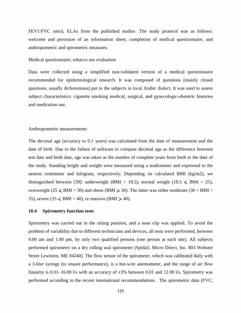
125

FEV1/FVC ratio), ELAs from the published studies .The study protocol was as follows:

welcome and provision of an information sheet; completion of medical questionnaire, and

anthropometric and spirometric measures.

Medical questionnaire, tobacco use evaluation

Data were collected using a simplified non-validated version of a medical questionnaire

recommended for epidemiological research. It was composed of questions (mainly closed

questions, usually dichotomous) put to the subjects in local Arabic dialect. It was used to assess

subject characteristics: cigarette smoking medical, surgical, and gynecologic-obstetric histories

and medication use.

Anthropometric measurements

The decimal age (accuracy to 0.1 years) was calculated from the date of measurement and the

date of birth. Due to the failure of software to compute decimal age as the difference between

test date and birth date, age was taken as the number of complete years from birth to the date of

the study. Standing height and weight were measured using a stadiometer and expressed to the

nearest centimeter and kilogram, respectively. Depending on calculated BMI (kg/m2), we

distinguished between [39]: underweight (BMI < 18.5), normal weight (18.5 ⩽ BMI < 25),

overweight (25 ⩽ BMI < 30) and obese (BMI ⩾ 30). The latter was either moderate (30 < BMI <

35), severe (35 ⩽ BMI < 40), or massive (BMI ⩾ 40).

10.4 Spirometry function tests

Spirometry was carried out in the sitting position, and a nose clip was applied. To avoid the

problem of variability due to different technicians and devices, all tests were performed, between

9.00 am and 1.00 pm, by only two qualified persons (one person at each site). All subjects

performed spirometry on a dry rolling seal spirometer (Spida5; Micro Direct, Inc. 803 Webster

Street Lewiston, ME 04240). The flow sensor of the spirometer, which was calibrated daily with

a 3-liter syringe (to ensure performance), is a hot-wire anemometer, and the range of air flow

linearity is 0.01–16.00 l/s with an accuracy of ±3% between 0.01 and 12.00 l/s. Spirometry was

performed according to the recent international recommendations . The spirometric data (FVC;

126

FEV1; FEFx (l/s), PEF (l/s), FEV1/FVC ratio (absolute value)) were expressed at “body

temperature, barometric pressure saturated with water vapor.” LLN for spirometric data was

calculated from the local spirometric norms. Any observed value for FEV1, FVC, and

FEV1/FVC ratio lower than its corresponding LLN was considered abnormal.

Data analysis:

Expression modes of results

The Kolmogorov–Smirnov test was used to analyze distribution of variables [30]. When the

distribution is normal and the variances are equal, the results are expressed by their mean ±

standard deviation (SD) and 95% confidence interval (95% CI). If the distribution is not normal,

the results are expressed by their medians (1st–3rd quartiles). The chi-2 test was used to compare

percentages. Preliminary descriptive analysis included frequencies for categorical variables (sex)

and mean ± SD (or median (1st–3rd quartiles)) for continuous ones (anthropometric and

spirometric data).

10.5 Published ELA reference equations (Box 1)

Morris and Temple have developed 6 reference equations models for the USA population aged

20–84 years. Newbury et al. have developed 2 reference equations models for the South

Australian population aged 25–74 years. Hansen et al. FEV1/FVC (%) for normal USA never-

smoking adults was independent of ethnicity and sex and equal to

98.8–0.25 × Age (years) — 1.79 × FVC

The EMIS predicted peak flow calculation used within its clinical systems is based on a

published revision to the original Nunn and Gregg equation in 1973. The revised Nunn and

Gregg equation is as below and applies to ages 15-85 years.

Male:

Loge (PEF) = 0.544 x loge (age) - 0.0151 x (age) - 74.7/ (height) + 5.48

Female:

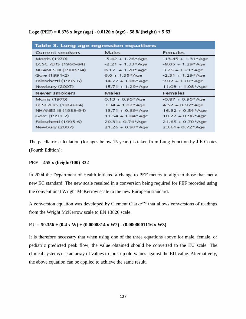
127

Loge (PEF) = 0.376 x loge (age) - 0.0120 x (age) - 58.8/ (height) + 5.63

The paediatric calculation (for ages below 15 years) is taken from Lung Function by J E Coates

(Fourth Edition):

PEF = 455 x (height/100)-332

In 2004 the Department of Health initiated a change to PEF meters to align to those that met a

new EC standard. The new scale resulted in a conversion being required for PEF recorded using

the conventional Wright McKerrow scale to the new European standard.

A conversion equation was developed by Clement Clarke™ that allows conversions of readings

from the Wright McKerrow scale to EN 13826 scale.

EU = 50.356 + (0.4 x W) + (0.0008814 x W2) - (0.0000001116 x W3)

It is therefore necessary that when using one of the three equations above for male, female, or

pediatric predicted peak flow, the value obtained should be converted to the EU scale. The

clinical systems use an array of values to look up old values against the EU value. Alternatively,

the above equation can be applied to achieve the same result.

128

129

Many physicians use spirometry to measure the lung function of smokers as a means to convince

them to stop smoking. If airflow obstruction is present (as evidenced by a reduction in FEV1.0),

this can be shown to the patient as evidence of the damage that cigarettes are doing to their

lungs. Rather than telling a patient that their lung function is x% reduced, it may have more

impact to tell the patient the age they would be for that lung function to be 100% predicted.

Telling a 55-year old male smoker that his lung function is that predicted for a 93-year old is

likely to be more eye-opening than telling him that his FEV 1.0 is 77% of predicted.

The accompanying predictive formula was derived from normal Caucasian subjects (Crapo RO

1981). It allows you to enter your patient's gender, height, and measured FEV1.0, then derive the

age for which that FEV1.0value is 100% predicted.

130

CONCLUSIONS AND IMPLICATIONS FOR

FURTHER RESEARCH:

The last word in the discussion on how to diagnose COPD is not said. We have contributed our

findings from paper 1 as mouse-steps in the right direction, but we do not expect agreement on

the most “fair” or reliable diagnose COPD. The human body can to some extent be classified

into mathematic stages, but it is not a machine. We must always treat each individual with

caution and relate the spirometric findings to the person treated. Probably future researchers have

to be more creative than researchers have been hitherto to find useful criteria. We may need to

create different criteria for different people in different age-groups. It is possible that we will

never can reach a worldwide agreement, and therefore have to find agreements within a country

or small parts of the world. Although symptoms are what all clinical doctors do navigate from,

symptoms in COPD cannot be the only reason for doing a spirometry. The most important

information for a doctor, when searching for COPD, is whether the patient smokes or not. If the

patient smokes the GP or the hospital doctor ought to start a conversation on smoking, and may

for instance ask for the smoking narrative, and encourage to have a spirometry taken. To help

smokers to stop is the most important issue to avoid getting COPD. More research, particularly

qualitative, is needed to find out more about smoking cessation. Is motivation as important as we

believe? What kind of processes must a smoker have gone through before she/he starts to

consider smoking cessation? Why do many smokers stop unplanned and unaided? How can we

best help the hardcore smokers? Lifestyle changes are difficult to handle, and much more

research is needed to understand the depth of the willingness to change. To effectively fight

tobacco we need a combination of strategies, both legislative, regulatory and public health. GPs

ought to learn different approaches to the smoking patients. Eliciting the smoking narrative as

method ought to be tested in practice, and implemented in clinical research to see if it adds more

to cessation than TTM, MI or 5As.

131

References

CONCLUSIONS AND IMPLICATIONS FOR

FURTHER RESEARCH

The last word in the discussion on how to diagnose COPD is not said. We have

contributed our findings from paper 1 as mouse-steps in the right direction, but we

do not expect agreement on the most “fair” or reliable diagnose COPD. The human

body can to some extent be classified into mathematic stages, but it is not a

machine. We must always treat each individual with caution and relate the

spirometric findings to the person treated. Probably future researchers have to be

more creative than researchers have been hitherto to find useful criteria. We may

need to create different criteria for different people in different age-groups. It is

possible that we will never can reach a worldwide agreement, and therefore have to

find agreements within a country or small parts of the world. Although symptoms

are what all clinical doctors do navigate from, symptoms in COPD cannot be the

only reason for doing a spirometry. The most important information for a doctor,

when searching for COPD, is whether the patient smokes or not. If the patient

smokes the GP or the hospital doctor ought to start a conversation on smoking, and

may for instance ask for the smoking narrative, and encourage to have a

spirometry taken. To help smokers to stop is the most important issue to avoid

getting COPD. More research, particularly qualitative, is needed to find out more

about smoking cessation. Is motivation as important as we believe? What kind of

processes must a smoker have gone through before she/he starts to consider

smoking cessation? Why do many smokers stop unplanned and unaided? How can

we best help the hardcore smokers? Lifestyle changes are difficult to handle, and

much more research is needed to understand the depth of the willingness to

change. To effectively fight tobacco we need a combination of strategies, both

legislative, regulatory and public health. GPs ought to learn different approaches to

the smoking patients. Eliciting the smoking narrative as method ought to be tested

in practice, and implemented in clinical research to see if it adds more to cessation

than TTM, MI or 5As.

References

[1] https://sites.google.com/site/team5spirometer/.

132

[2] http://www.hopkinsmedicine.org/healthlibrary/test_procedures/pulmonary/p

ulmonary_function_tests_92,P07759/.

[3] http://www.maximintegrated.com/en/site-map.html.

[4] http://www.hindawi.com/journals/ijfm/2014/962901/.

[5] http://www.nursingtimes.net/nursing-practice/clinical-zones/copd/improving-

early-detection-of-copd-the-role-of-spirometry-screening-

assessment/199956.article.

[6] https://www.labviewhacker.com/doku.php?id=projects:lv_kinect_interface:lv

_kinect_interface.

[7] http://www.ni.com/

[8] Aston, Richard; Principles of Biomedical Instrumentation and Measurement;

Merrill, Columbus Ohio, 1990.

[9] Bronzino, Joseph D; Biomedical Engineering and Instrumentation: basic

concepts and applications; PWS Engineering, Boston, 1986.

[10] Pierce, Rob; Johns, David P. Spirometry Handbook. The measurement and

interpretation of ventilator function in clinical practice; McGraw-Hill,

Australia, 2007.

[11] Profio, A. Edward; Biomedical Engineering; Wiley, New York, 1993.

[12] Savant, C. J.; Diseño electronic:, circuitous y systems; Pearson Education,

México, 2000.

[13] Webster, John G.; Encyclopedia of Medical Devices and Instrumentation;

Vol. 4, Wiley, New York, 1998.

[14] Webster, John G.; Medical Instrumentation: application and Design; Wiley,

New York, 1998.

[15] FLOW SPIROMETER Sergio Quintana T., Ricardo Damián Z., José Castillo

H., Gibrán Mejía T.

[16]http://in.element14.com/freescale-emiconductor/mpx5050dp/ic-pressure

-sensor/dp/1555606

[17]http://www.xilinx.com/support/documentation/application_no

tes/xapp462.pdf

[18] http://www.comsol.co.in/

[19] http://www.ni.com/labview/

133

[20] https://wiki.cites.illinois.edu/