Design and control of an altazimuth liquid mirrortelescope

Juan Cristobal Alcaraz Tapia1, Carlos E. Castaneda2, and Hector Vargas-Rodrıguez3

Abstract—In this paper, it is considered the design of atelescope in an altazimuth configuration. Its primary objective isa rotating liquid mirror made of mercury (any rotating liquidnaturally adopts a perfect paraboloidal shape). This liquid mirrorcannot be oriented. Hence, a mechanical and optical system isneeded to conduct the light of a celestial body to it. The lattersystem is composed of two plane mirrors which, rotate arounda horizontal and a vertical axis, two motors are employed tofulfill this purpose. The non-linear-block-control method is usedto control these motors. A third motor keeps-up rotating acontainer filled with mercury to form the liquid mirror, the focallength of the rotating mirror depends on the angular velocityof this last motor. Hence, its rotation rate also needs to becontrolled. The Methodology’s part A describes the design ofa 2-links mechanical and optical system. The Methodology’spart B introduces the gravitational potential and the kineticenergy for each link in the mechanical and optical system. Then,using the Euler-Lagrange formalism, the equations governingthis mechanical and optical system are obtained. Next, in theMethodology’s part C, a nonlinear block control strategy is usedto synthesize the control algorithm for the mechanical and opticalguide system. Finally, a stability analysis is performed, using theLyapunov criterion.

The obtained results are presented via simulation using thesoftware Simulinkr.

Index Terms—Liquid mirror telescope, star tracking system,non-linear block control, telescope movement.

I. INTRODUCTION

THERE have been various articles about liquid mirrors inthe last 35 years since [1], which mentions the usefulness

of these liquid mirrors in a telescope for a specific type of ob-servations. This kind of applications is possible due to electro-optical tracking that, can be achieved thanks to the adventof charge-coupled devices (CCD) detectors. The firsts liquidmirror telescopes (LMT’s) like the NASA’s orbital debrisobservatory (NODO) [2] used CCD detectors, as well as themodern like the 4m International Liquid Mirror Telescope, willuse [3]. LMT’s were not taken seriously before using CCD’s,because the liquid mirror cannot tilt in order to track a star. Asa result, while stars move apparently in the sky, a film in thetelescope register them as streaks. The use of a CCD detectorsolves this problem by moving its light sensors electronicallyfrom the east to the west, at a rate matching the drift of imagesin view of the telescope. This is equivalent to taking a picturewith a photographic film that moves in a camera at the same

J. C. Alcaraz, Carlos E. Castaneda and Hector Vargas arewith Departamento de Ciencias Exactas y Tecnologıa, CentroUniversitario de los Lagos, Universidad de Guadalajara, MEX e-mail:1cristobal.alcaraz@alumnos.udg.mx, 2ccastaneda@lagos.udg.mx,3hvargas@culagos.udg.mx.

speed as the image of a moving object. Tipically in only acouple of minutes, an object crosses the narrow width of thedetector, limiting the amount of light that can be gathered.Observing the same region of the sky night after night, itis possible to create increasingly intense images by digitallyadding subsequent exposures on a computer [4]. Even with itsrestriction to the zenith, Liquid Mirror Telescopes (LMT’s) arestill very appropriate for many survey applications, includinglarge-scale structure, galaxy evolution, depth of a Quasi-stellar object (QSO), galaxy surveys, etc. Therefore, the LMTdesign is directed towards those applications which need largesamplings of data, not necessarily from any specific directionin space [5]. The Large Zenith Telescope [6] is proof ofthis, it was built with a budget of more than an order ofmagnitude lower than that of conventional telescope projectsof a comparable aperture. Even it has been presented thefeasibility and scientifical potential of a 20-100 m apertureastronomical LMT constructed in one of the lunar poles [7].And there are projects under development among them theAdvanced Liquid-Mirror Probe for Astrophysics, Cosmology,and Asteroids (ALPACA) and the International Liquid-MirrorTelescope (ILMT) [6]. This last one is under construction.

On the other hand, when a container filled with a liquidis rotated, the pull of gravitational and centrifugal forcesshapes the surface of the liquid into a perfect parabola [4].The shape of the objectives in conventional telescopes is aparabola, so rotating a container with a reflecting liquid, suchas mercury, results in a liquid mirror with a perfect shape for atelescope’s objective. In fact in [8] the quality of astronomicalimages provided by the NODO and the LZT was assessed andcompared to that of conventional instruments, concluding theimages provided by the LMT’s are of scientific quality.The focal length l of the liquid mirror is given by:

l =g

2ω2, (1)

for a given value of the acceleration of gravity g, the focallength is determined by the angular velocity ω [1]. As provedby Borra [4], the surface made by a liquid mirror can beperfectly parabolic and limited diffracted. There are otheruses besides astronomical ones for a liquid mirror such asatmospheric science or in a telecentric F-Θ scanner with alow-cost liquid mirror objective [9].

II. PROPOSED METHODOLOGY

A. Liquid mirror telescope design

As mentioned in the previous section, LMT’s cannot tilt,and as a consequence, they cannot follow a celestial object in

NTERNATIONAL JOURNAL OF MATHEMATICAL MODELS AND METHODS IN APPLIED SCIENCES Volume 12, 2018

ISSN: 1998-0140 112

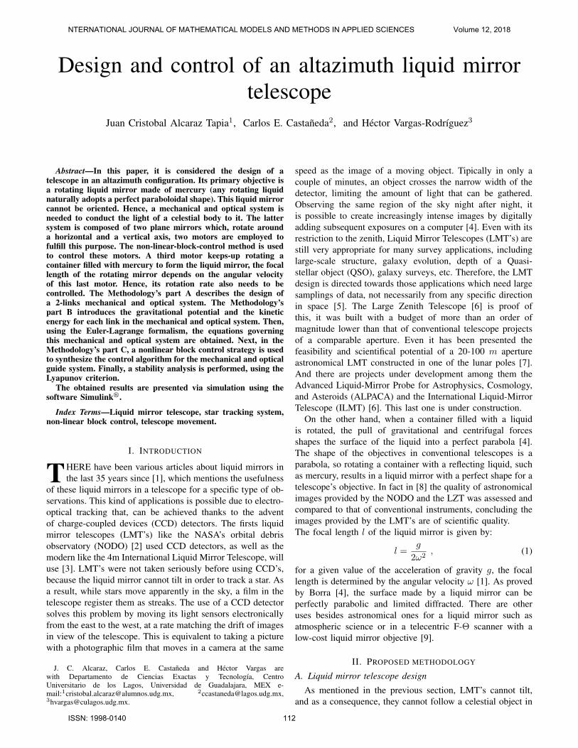
the sky. In order to overcome this inconvenient, this subsectiondescribes the design of an orientable LMT. Fig. 1 shows themain elements of the LMT and Table I lists every componentshown in this figure.

1

1 SECTION 1-1

2

3

1

SCALE DETAIL 1 : 5

4

5

Fig. 1. Design and main elements of the tiltable LMT.

TABLE ILIQUID MIRROR TELESCOPE’S MAIN COMPONENTS OF FIGURE 1.

No.of element Piece Quantity

1 Plane mirror 22 Motor 23 Counterweight 24 Container with liquid mercury 15 Air bearing 1

The two plane mirrors direct the light to the liquid mirror.One of these plane mirrors is rotating around the horizontalaxis, while the other one around the vertical axis; both ofthem along with the pipe containing them. The sketch in Fig.2 shows this path of the light inside the telescope from thesource to the ocular. In this figure, the light is represented byrays in order to describe its path inside the telescope; first, theincoming light is reflected along the horizontal pipe, then theother flat mirror redirects the light to the liquid mirror. Theplane mirrors are tilted 45◦ with respect to the pipes’ axis,then vertical rays are reflected horizontally, and vice versa.Fig. 3 contains a 3d-model of the proposed design and therange of movement of the links of the telescope.

The coordinates of a star in the celestial sphere are calleddeclination (δ) and right ascension (R.A.), these are knownas equatorial coordinates [10]. The telescope proposed is inan altazimuth configuration, so, it is necessary to convertequatorial coordinates of the star (R.A. and δ) to horizoncoordinates (q1 and q2 (Fig. 4)) of the telescope in order totrack the reference (the movement of a star).

B. Kinematics and dynamics

Before we design a control strategy, it is necessary to havea dynamic model to which apply it for simulation purposes; in

Fig. 2. Reflection of the light inside the telescope.

Fig. 3. Telescope’s range of movement.

this case, the dynamic model of the telescope proposed. Thepresent subsection describes the obtention of the dynamics,

NTERNATIONAL JOURNAL OF MATHEMATICAL MODELS AND METHODS IN APPLIED SCIENCES Volume 12, 2018

ISSN: 1998-0140 113

by the use of the Euler-Lagrange equations. The functionrequired to obtain the dynamics is the Lagrangian. Thisfunction is the difference between the kinetic and potentialenergy of the mechanical model of the proposed telescope.For the calculation of kinetic energy, the linear velocity ofeach link of the telescope is needed. The linear velocity isrepresented as a function of joint velocity, this function isknown as differential kinematics, which is the derivative withrespect to time of a function called direct kinematics. Directkinematics is a function of the joint variable (q). So, beforeobtaining the dynamic model of the proposed telescope and toapply a control strategy, the direct kinematics and differentialkinematics will be required.

1) Direct kinematics: The mechanical structure of the tele-scope proposed has n = 2 degrees of freedom, each one isassociated with one joint articulation. Then, this subsectiondescribes the direct kinematics of the proposed telescope. Theaim of direct kinematics is to compute the position of the lastlink as a function of the joint variable [11]; that is, fR(q)where q is the joint variable. There are various methods todetermine the direct kinematics model, but a first way todetermine it is by applied geometry [11]. Another methodis the Denavit-Hartenberg convention [12], which is moreconvenient for a greater number of degrees of freedom becauseis a systematic method. Using the last one mentioned, it isobtained the direct kinematics of the telescope’s mechanicmodel shown in Fig. 4, using the symbolic values presentedin Table II, where l1 and l2 are the lengths of links 1 and2 starting from their rotation axes; B1 is the offset fromthe origin of the inertial frame to the rotation axis of thelink 2; B2 is the distance from the end of link 1 to thecenter of link 2; q1 and q2 are the rotation angles of links1 and 2, respectively; and α is the angle between the rotationaxis for link 1 (Z1) and the rotation axis for link 2 (Z2).So, the Denavit-Hartenberg representation for link 1, throughhomogeneous transformations is as follows:

H10 = Rz,q1Tz,d1Tx,l1Rx,α1

=

cos q1 0 sin q1 l1 cos q1sin q1 0 − cos q1 l1 sin q1

0 1 0 B1

0 0 0 1

(2)

where Rz,q1 and Rx,α1 are rotation homogeneous transforma-tion around axes Z and X of the link in question, respectively;Tz,d1 and Tx,l1 are translation homogeneous transformation;and H1

0 is the homogeneous transformation relationing thecoordinates in the reference system of link 1 and the referencesystem at the base of the telescope, as it is shown in Fig. 4[13]. In equation (2), the rows 1-3 in the column 4, representthe position [X0, Y0, Z0]> of the end of link 1 as follows:X0

Y0

Z0

=

l1 cos q1l1 sin q1B1

. (3)

Continuing with the Denavit-Hartenberg convention on link2, we obtain H2

0 = H21H

10 . It is important to mention that

the direct application of the Denavit-Hartenberg convention

Fig. 4. Telescope’s mechanic model

TABLE IISYMBOLIC VALUES FOR THE PROPOSED TELESCOPE.

Link Lenght(m)

Angle betweenrotation axes (rad)

Offset(m)

Rotation angles(rad)

1 l1π2

B1 q12 l2 0 B2 q2

for link 2 leads to the reference system [X′2, Y2, Z′2]> shownin Fig. 4. This would be true if the two links were parallelsbecause the X1 and X2 axes are along the length of theircorresponding link. But links 1 and 2 form a right angle; so,in order to represent this configuration of links, it is necessaryto rotate link 2 around the Y2 axis an angle of π

2 rads. Thisconduces to the reference system of link 2 [X2, Y2, Z2]>. Forthe rotation, it is used a rotation homogeneous transformationaround the axis Y2; and the position vector for the end of link2 is:X0

Y0

Z0

=

B2 cos(q1) + l1 cos(q1)− l2 cos(q2) sin(q1)B2 sin(q1) + l1 sin(q1) + l2 cos(q1) cos(q2)

B1 + l2 sin(q2)

.(4)

Then, the direct kinematics of each link in the mechanicmodel of the proposed telescope is represented by equations(3) and (4), which are in function of the joint variables q1 andq2.

2) Differential kinematics: The differential kinematicsgives the relationship between joint velocity q and the linealvelocity v [11], [14]; then:

d

dt

XYZ

=d

dtfR(q) =

∂fR(q)

∂qq = J(q)q = v , (5)

where [X Y Z]> is the position vector as a function of the jointvariable obtained by the direct kinematics (equations (3) and(4)), J(q) is the Jacobian of the robot or analytical Jacobian[14], and fR(q) is a function of the joint variable q.

The lineal velocity v1 of the center of mass (cm) corre-sponding to the link 1 is obtained as follows:

v1 =d

dt

l1cm cos q1l1cm sin q1

B1

=

−l1cm sin q1l1cm cos q1

0

q1 . (6)

NTERNATIONAL JOURNAL OF MATHEMATICAL MODELS AND METHODS IN APPLIED SCIENCES Volume 12, 2018

ISSN: 1998-0140 114

The linear velocity of the center of mass corresponding to thelink 2 is obtained as:

v2 =d

dt

B2 cos q1 + l1 cos q1 − l2cm cos q2 sin q1B2 sin q1 + l1 sin q1 + l2cm cos q1 cos q2

B1 + l2cm sin q2

=

v2 11 l2cm sin q2 sin q1v2 21 −l2cm cos q1 sin q2

0 l2cm cos q2

[q1q2

] , (7)

where v2 11 = −B2 sin q1 − l1 sin q1 − l2cm cos q2 cos q1 andv2 21 = B2 cos q1 + l1 cos q1 − l2cm sin q1 cos q2.Equations (6) and (7) represent the linear velocity for links 1and 2, respectively; now, it is possible to compute the kineticenergy needed for the dynamics, which it is shown in sectionII-B3.

3) Dynamics: Now, it is necessary to determine the equa-tions of motion of the proposed telescope design; this isin order to propose control strategies that can be tested forsimulation purposes. The method chosen in this paper todetermine the dynamic equations of the telescope is the use ofthe Euler-Lagrange equations. In order to determine the Euler-Lagrange equations, it is necessary to obtain the Lagrangian ofthe system, which is the difference between the kinetic energyand the potential energy [15] as follows:

L(q, q) = K(q, q)− U(q) (8)

where L(q, q) is the Lagrangian, K(q, q) is the kinetic energy,and U(q) the potential energy.

It is important to mention that the proposed telescope hasthe configuration of the two degrees of freedom (DOF) robotmanipulator. Then, the Euler-Lagrange equation of motion forthe n DOF is:

d

dt

[∂L(q, q)

∂q

]− ∂L(q, q)

∂q= τ − ff (q,fe) (9)

The equation (9) can be written in the following form:

τ = M(q)q+M(q)q− ∂

∂q

[1

2q>M(q)q

]+∂U(q)

∂q+ff (q,fe),

(10)which, in its compact form and with the most widely usednotation in the area of robotics [14], [11] is described asfollows:

τ = M(q)q + C(q, q)q +G(q) + ff (q,fe), (11)

where τ ∈ Rn is the vector of applied torques, q ∈ Rn is thevector of generalized coordinates or joint positions, q ∈ Rnis the vector of joint velocities and q ∈ Rn is the vector ofjoint accelerations. M(q) ∈ Rn×n is the inertia matrix, whichis symmetric and positive definite, C(q, q) ∈ Rn×n is thematrix of centripetal and Coriolis forces, which is defined asfollows:

C(q, q)q = M(q)q − ∂

∂q

[1

2q>M(q)q

],

G(q) ∈ Rn is the vector of gravitational forces obtained asthe gradient of the potential energy, this is:

G(q) =∂U(q)

∂q,

and ff (q,fe) ∈ Rn is the vector of friction forces thatincludes the viscous, Coulomb and static friction (fe) of eacharticulation.

The function K(q, q) includes rotational and translationalkinetic energy [14]:

Ki(q, q) =1

2miv

>i vi +

1

2Ii

[n∑i

qi

]2, i = 1, ..., n, (12)

with n = 2 as the number of DOF, and where mi and Ii arethe mass and moment of inertia of the i-th, respectively. Themoment of inertia of the i-th link is around an axis that passesthrough its center of mass and is parallel to the rotation axisaround which the link rotates [15].Then, using the equation (12), the kinetic energies for link 1and link 2 are:

K1 =1

2m1v

>1 v1 +

1

2I1q

21 , (13)

K2 =1

2m2v

>2 v2 +

1

2I2(q1 + q2)2. (14)

From equations (6) and (7), it can be obtained v>1 v1 and v>2 v2,respectively as:

v>1 v1 = (l1cmq1)2, (15)

v>2 v2 = [(B2 cos(q1) + l1 cos(q1)− l2cm cos(q2) sin(q1))q1

(−l2cm cos(q1) sin(q2)q2)]2

+ [B2 sin(q1) + l1 sin(q1) + l2cm cos(q1) cos(q2)q1

− l2cm sin(q1) sin(q2)q2]2

+ [l2cm cos(q2)q2].(16)

The total kinetic energy is:

K(q, q) = K1 +K2. (17)

Unlike the kinetic energy, the potential energy does not have aspecific form. It depends on the geometry of the robot (for ourparticular case, the proposed telescope). The potential energyfor links 1 and 2 is:

U1 = m1gB1, (18)

U2 = m2g(B1 + l2cm sin q2). (19)

The total potential energy is:

U(q) = U1 + U2. (20)

In order to obtain the Lagrangian, the kinetic (17) and potential(20) energy are substitued in equation (8), and the Euler-Lagrange’s equation of motion (9) can be obtained. The resultcan be represented as in equation (11), where the entries ofthe inertia matrix M(·) are:

M11 = I1 + I2 + l21m2 + l21cmm1

+B22m2 + l22cmm2 cos2(q2) + 2B2l1m2

M12 = I2 −B2l2cmm2 sin(q2)− l1l2cmm2 sin(q2)

M21 = I2 −B2l2cmm2 sin(q2)− l1l2cmm2 sin(q2)

M22 = I2 + l22cmm2.

(21)

NTERNATIONAL JOURNAL OF MATHEMATICAL MODELS AND METHODS IN APPLIED SCIENCES Volume 12, 2018

ISSN: 1998-0140 115

The entries in the matrix of centripetal and Coriolis forcesC(·) are:

C11 = −(l22cmm2 sin(2q2)q2)

C12 = [−B2l2cmm2 cos(q2)− l1l2cmm2 cos(q2)] q2

C21 = l22cmm2 cos(q2) sin(q2)q1

C22 = 0.

(22)

The entries in the vector of gravitational forces G(·) are:

G11 = 0

G21 = gl2cmm2 cos(q2).(23)

The entries in the vector of friction forces ff (·) are:[ff1(q1, fe1)ff2(q2, fe2)

]= Bq + Fc sign(q)

+

[1− |sign(q1)| 0

0 1− |sign(q2)|

]fe

.

(24)where B and Fc ∈ Rn×n are diagonal matrices with viscousand Coulomb friction coefficient, respectively. fe is the vectorof static friction and sign(q) = [sign(q1), sign(q2)]

>.Then, the dynamic equations of the model of the telescopecan be represented in the state space as follows:[

x1x2

]=

[x3x4

][x3x4

]= N

[U − C

[x3x4

]−G− ff

],

(25)

where

N = M−1,

x1x2x3x4

=

q1q2q1q2

, U =

[u1u2

]=

[τ1τ2

].

Now, with the dynamic equation of the proposed telescoperepresented in state space (25), a strategy of control can beapplied.

C. Control design

In this section, it is proposed a non-linear block controlalgorithm in order to the telescope tracks a star movement.

1) Telescope control design: For this paper, model (25) canbe represented as a non-linear block controllable form (NBC-form) [16], which is represented by two blocks:

X 1 = X 2

X 2 = f2(X 1,X 2) +D(X 1)U(26)

whereX 1 =

[x1x2

], X 2 =

[x3x4

], (27)

f2(·) = N[−C

[x3x4

]−G− ff

]=

[N11 [−C11x3 − C12x4 −G11 − ff1]N21 [−C11x3 − C12x4 −G11 − ff1]

+N12 [−C21x3 −G21 − ff2]+N22 [−C21x3 −G21 − ff2]

],

(28)

and

D(·) = N (29)

The error E1 (E2) is the difference between the block X 1 (X 2)(27) and the reference signal to be tracked X 1

d (X 2d ). Note that

signals X 1d and X 2

d are the joint angle and joint velocity ofeach link of the telescope, respectivaly, needed to keep a starin sight. Then E1 and E2 are represented as follows:

E1 = X 1 −X 1d , (30)

E2 = X 2 −X 2d , (31)

where

X 1d =

[x1dx2d

]=

[270−A

a

], (32)

and [aA

]=

sin−1(sin δ sinφ+ cos δ cosφ cosH)

cos−1(

sin δ − sinφ sin a

cosφ cos a

) . (33)

The equation (33) shows the relation between the hour-angleH , the declination δ, the observer’s geographical latitude φ,the azimuth A, and the altitude a [17], and X 2

d = [x3d x4d]>.

The azimuth angle A increases in the opposite way of q1,starting from the north. If “X” in Fig. 4 points to the north,then, when the angle q1 = 0, the link 2 of the telescope pointsto the west (axis Y). Taking this into account, it is easy toobtain the relation between these angles (q1 = 270◦-A).

The dynamics of E1 and E2 is:

E1 = X 1 − X 1d , (34)

E2 = X 2 − X 2d . (35)

Substituting the first equation of (26) in (34), yields:

E1 = X 2 − X 1d . (36)

Imposing the desired dynamics K1E1 in (36), by choosing thedesired value for the virtual control X 2

d [18], it is obtained:

K1E1 = X 2d − X 1

d . (37)

Then

X 2d = K1E1 + X 1

d . (38)

The time derivative of X 2d is described by the following

equation:

X 2d = K1E1 + X 1

d . (39)

Taking the value of X 2 in (31), and the value of X 2d in (38),

and substituting them in (36), it is obtained:

E1 = E2 + X 2d − X 1

d

= K1E1 + E2.(40)

NTERNATIONAL JOURNAL OF MATHEMATICAL MODELS AND METHODS IN APPLIED SCIENCES Volume 12, 2018

ISSN: 1998-0140 116

Now, for the dynamics of E2, substituting X 2, X 2d , X 2

d , X 1,X 2 and E1 from equations (26), (38), (39), (30), (31) and (40),respectively in equation (35), it is obtained:

E2 = X 2 − X 2d

= f2(X 1,X 2) +D(X 1)U − X 2d

= f2(E1 + X 1d , E2 + X 2

d ) +D(E1 + X 1d )U −K1E1 − X 1

d

= f2(E1 + X 1d , E2 +K1E1 + X 1

d ) +D(E1 + X 1d )U

−K1(K1E1 + E2)− X 1d .

(41)

The equation of system (26) is transformed to the blockcontrollable form using the error dynamics as follows:

E1 = K1E1 + E2

E2 = f2(E1 + X 1d , E2 +K1E1 + X 1

d ) +D(E1 + X 1d )U

−K1(K1E1 + E2)− X 1d .

(42)Then, imposing the desired dynamics for E2 = K2E2 in (41),the control signal U is defined by:

U =M(E1 + X 1d )[−f2(E1 + X 1

d , E2 +K1E1 + X 1d )

+K1(K1E1 + E2) + X 1d +K2E2

].

(43)

As it can be seen in equation (43), the control lawU is in func-tion of the errors E1 (30), E2 (31), and the desired referenceX 1d (32) including its first and second time derivatives (X 1

d

and X 1d ). For the particular case of the present proposal, this

reference signal varies in time due to the apparent movementof the stars in the sky, so, these derivatives exist. In fact,the first derivative is the rotation rate for each motor thatcontrols the rotation of each link, and the second derivative isits angular acceleration.

2) Angular velocity control of the liquid mirror motor:As mentioned earlier, for varying the focal length of a liquidmirror, it is necessary to control the angular velocity of therecipient that contains the liquid mirror. The equation (1)represents the relation between angular velocity and the focallength. So, it is needed to apply a control algorithm to themodel of a motor, which has to keep rotating the containermentioned at a constant velocity. In this work, the trackingof the angular velocity of the motor is accomplished by theuse of the state-feedback linearization technique applied to aDC motor model, just as it is shown in reference [19]. Thisis in order to keep the focal length of the mirror in a desiredvalue depending on the observations that will be done withthe telescope.

D. Stability analysis

For the stability analysis, it is used the state space equationin terms of the errors (E1, E2). This state space equation isrepresented by equation (40), and the result of substitute thecontrol law (43) in (41) yields the following linear represen-tation in state space:

E1 = K1E1 + E2

E2 = K2E2=

[K1 10 K2

] [E1E2]

(44)

Each row in equation (44) is a block, so expanding each ofthese, results in:

E1E2E3E4

=

k1 0 1 00 k2 0 10 0 k3 00 0 0 k4

E1E2E3E4

(45)

then, as it is explained in [20], the origin is asymptoticallystable if Reλi < 0 for all eigenvalues of the state matrix in(45); this is, the state matrix in (45) is a Hurwitz matrix orstability matrix. The eigenvalues of the state matrix in (45)are:

λ1 = k1

λ2 = k2

λ3 = k3

λ4 = k4.

(46)

The coefficients k1, k2, k3, k4 comes from:

K1 =

[k1 00 k2

], K2 =

[k3 00 k4

]For a linear equation system like (45), it is considered thefollowing quadratic Lyapunov function candidate [20]:

V (x) = x>Px (47)

The derivative of (47) is given by:

V (x) = x>Px+ x>Px = −x>Qx (48)

where Q is defined by:

PA′ +A′>P = −Q (49)

Then, a matrix A′ is Hurwitz if and only if for any givenpositive definite symmetric matrix Q there exists a positivedefinite symmetric matrix P that satisfies the Lyapunov equa-tion (49). Moreover, if A′ is Hurwitz, then, the matrix P isunique [20]. Choosing Q as a real symmetric positive definitematrix (in this case the identity matrix), and solving for P , itis obtained:

P =

− 1

2k10 1

2k1(k1+k3)0

0 − 12k2

0 12k2(k2+k4)

12k1(k1+k3)

0 P3,3 0

0 12k2(k2+k4)

0 P4,4

(50)

with:

P3,3 = − k21 + k1k3 + 1

2k1k3(k1 + k3)and P4,4 = − k22 + k2k4 + 1

2k2k4(k2 + k4).

The matrix P (50) is positive definite if and only if allits leading principal minors are positive (which it is trueif the values of k1, k2, k3, k4 are negative), and since Qis also definite positive we can conclude that the origin isasymptotically stable [20].

NTERNATIONAL JOURNAL OF MATHEMATICAL MODELS AND METHODS IN APPLIED SCIENCES Volume 12, 2018

ISSN: 1998-0140 117

III. RESULTS

A. Direct kinematics

Focusing only on link 1, it is easy to verify that theposition vector (3) is correct, without the need of usingthe Denavit-Hartenberg convention. Link 1 rotates arounda vertical axis Z, then its height does not vary, its positionX is equal to the product of the length from the origin tothe end of the link and the cosine of the angle q1; thus, theposition Y is equal to the product of the length l1 and thesine of q1. The position vector (4) is a little more complex toanalyse, but it is more clear with the Figs. 5 and 6 and usingthe following values: l1 = l2 = 0.10 m, B1 = 1.00 m andB2 = 0.05 m for different angles q1 and q2.Figs. 5 and 6 show that when the angle q1 turns a completeturn and the angle q2 is fixed (Fig. 5), the end of link 2starts on an X position l1 + B2 = 0.15 m, a Y positionl2 = 0.1 m, and the Z position does not change (staysin B1 = 1.00 m). Now, when q1 is fixed and q2 turns acomplete turn (Fig. 6), the position X does not change (staysin l1 +B2 = 0.15 m), the Y position reaches a maximum andminimum of l2 = 0.10 m and −l2 = −0.10 m, respectively,and the Z position reaches a maximum and minimum valueof B1 ± l2 = 1.00 m ± 0.1 m, respectively. These valuescorrespond to the positions X, Y, and Z of the end of link 2,as it is shown in Fig. 4.

Fig. 5. Position X, Y and Z: q1 turns a complete turn and q2 is fixed.

Fig. 6. Position X, Y and Z: q1 is fixed and q2 turns a complete turn.

B. Star tracking performance

By applying the Non-linear block control for the telescope’sdynamic model, thus, using the control input vector obtained

in equation (43), a signal reference (in this case the movementof a star (32)) can be tracked. It is required this reference (X 1

d ),its derivative (X 1

d ), and second derivative (X 1d ). The entries of

equation (32) are the desired angles q1 and q2 for the links 1and 2, respectively, needed for tracking a star.

In this work it is used the data for the star Altair (R.A.= 19h50min 47sec, δ = 8◦52′6′′) [21] in order to be tracked by thetelescope proposed. The observation is considered from a placewith latitude 21.36◦, starting the tracking when the star is atthe observer’s zenith and for 4 hours (sidereal time). Figs. 7and 8 show the tracking performance for angles q1 and q2,respectively. In both figures there is a detail that includes 10seconds (sidereal time) of simulation, demonstrating the fastconvergence given in two seconds approximately.

The signal references (x1d and x2d (32)) from Figs. 7 and 8,are obtained by converting equatorial to horizon coordinates,as it is explained in [17].

It is important to mention that the time in the graphics issidereal time, and each hour-angle corresponds to 15 degreesfrom the observer’s zenith to the star being observed. Then, 24hours-angle corresponds to 360 degrees. The simulation timeof Figs. 7 and 8 correspond to 3h 59min 20sec of solar time.

0 0.5 1 1.5 2 2.5 3 3.5 4Hour-angle

-0.2

0

0.2

0.4

0.6

0.8

1

1.2

1.4

Rad

Detail

0 2 4 6 8 10 Seconds (sidereal time)

0

0.5

1

1.5

Rad

Fig. 7. Angular position tracking performance for q1.

0 0.5 1 1.5 2 2.5 3 3.5 4Hour-angle

-0.2

0

0.2

0.4

0.6

0.8

1

1.2

1.4

Rad

Detail

0 2 4 6 8 10 Seconds (sidereal time)

0

0.5

1

1.5

Rad

Fig. 8. Angular position tracking performance for q2.

C. Liquid mirror’s focal length tracking performance

As mentioned above, the liquid mirror in the telescopevaries its focal length along with its angular velocity in arelationship described by equation (1). So, in order to keepa steady focal length, it is necessary to maintain a steadyvelocity.Fig. 9 shows the control of the rotation of a DC motor trackingthe angular velocity (reference) needed to maintain a focal

NTERNATIONAL JOURNAL OF MATHEMATICAL MODELS AND METHODS IN APPLIED SCIENCES Volume 12, 2018

ISSN: 1998-0140 118

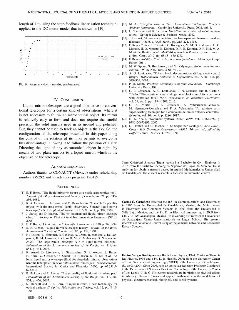
length of 1 m using the state-feedback linearization technique,applied to the DC motor model that is shown in [19].

Fig. 9. Angular velocity tracking performance.

IV. CONCLUSION

Liquid mirror telescopes are a good alternative to conven-tional telescopes for a certain kind of observations, where itis not necessary to follow an astronomical object. Its mirroris relatively easy to form and does not require the carefulprecision the solid mirrors need in its ground and polished.But, they cannot be used to track an object in the sky. So, theconfiguration of the telescope presented in this paper alongthe control of the rotation of its links permits to overcomethis disadvantage, allowing it to follow the position of a star.Directing the light of any astronomical object in sight, bymeans of two plane mirrors to a liquid mirror, which is theobjective of the telescope.

ACKNOWLEDGMENT

Authors thanks to CONACYT (Mexico) under scholarshipnumber 779292 and to retention program 120489.

REFERENCES

[1] E. F. Borra, “The liquid-mirror telescope as a viable astronomical tool,”Journal of the Royal Astronomical Society of Canada, vol. 76, pp. 245–256, 1982.

[2] R. A. Cabanac, E. F. Borra, and M. Beauchemin, “A search for peculiarobjects with the nasa orbital debris observatory 3 meter liquid mirrortelescope,” The Astrophysical Journal, vol. 509, no. 1, p. 309, 1998.

[3] J. Surdej and D. Mawet, “The 4m international liquid mirror telescope(ilmt).” Society of Photo-Optical Instrumentation Engineers (SPIE),2006.

[4] E. F. Borra, “Liquid mirrors,” Scientific American, vol. 270, p. 76, 1994.[5] B. K. Gibson, “Liquid mirror telescopes-history,” Journal of the Royal

Astronomical Society of Canada, vol. 85, p. 158, 1991.[6] P. Hickson, T. Pfrommer, R. Cabanac, A. Crotts, B. Johnson, V. De Lap-

parent, K. M. Lanzetta, S. Gromoll, M. K. Mulrooney, S. Sivanandamet al., “The large zenith telescope: A 6 m liquid-mirror telescope,”Publications of the Astronomical Society of the Pacific, vol. 119, no.854, p. 444, 2007.

[7] R. Angel, D. Eisenstein, S. Sivanandam, S. P. Worden, J. Burge,E. Borra, C. Gosselin, O. Seddiki, P. Hickson, K. B. Ma et al., “Alunar liquid mirror telescope (llmt) for deep-field infrared observationsnear the lunar pole,” in SPIE Astronomical Telescopes+ Instrumentation.International Society for Optics and Photonics, 2006, pp. 62 651U–62 651U.

[8] P. Hickson and R. Racine, “Image quality of liquid-mirror telescopes,”Publications of the Astronomical Society of the Pacific, vol. 119, no.854, p. 456, 2007.

[9] S. Thibault and E. F. Borra, “Liquid mirrors: a new technology foroptical designers,” Optical Fabrication and Testing, vol. 12, pp. 8–10,1998.

[10] M. A. Covington, How to Use a Computerized Telescope: PracticalAmateur Astronomy. Cambridge University Press, 2002, vol. 1.

[11] L. Sciavicco and B. Siciliano, Modelling and control of robot manipu-lators. Springer Science & Business Media, 2012.

[12] J. Denavit, “A kinematic notation for lower-pair mechanisms based onmatrices,” ASME J. Appl. Mech., pp. 215–221, 1955.

[13] F. Reyes Cortes, F. R. Cortes, G. Rodriguez, M. M. G. Rodriguez, H. O.Moratto, H. O. Moratto, B. Kolman, D. R. B. Kolman, D. R. Hill, M. A.Montufar Benıtez et al., MATLAB aplicado a Robotica y mecatronica.e-libro, Corp., 2012, no. 681.51 670.4272.

[14] F. Reyes, Robotica-Control de robots manipuladores. Alfaomega GrupoEditor, 2011.

[15] M. W. Spong, S. Hutchinson, and M. Vidyasagar, Robot modeling andcontrol. Wiley New York, 2006, vol. 3.

[16] A. G. Loukianov, “Robust block decomposition sliding mode controldesign,” Mathematical Problems in Engineering, vol. 8, no. 4-5, pp.349–365, 2002.

[17] P. D. Smith, Practical astronomy with your calculator. CambridgeUniversity Press, 1981.

[18] C. E. Castaneda, A. G. Loukianov, E. N. Sanchez, and B. Castillo-Toledo, “Discrete-time neural sliding-mode block control for a dc motorwith controlled flux,” IEEE Transactions on Industrial Electronics,vol. 59, no. 2, pp. 1194–1207, 2012.

[19] O. A. Morfin, C. E. Castaneda, A. Valderrabano-Gonzalez,M. Hernandez-Gonzalez, and F. A. Valenzuela, “A real-time sosmsuper-twisting technique for a compound dc motor velocity controller,”Energies, vol. 10, no. 9, p. 1286, 2017.

[20] H. K. Khalil, “Nonlinear systems. 2002,” ISBN, vol. 130673897, p.9780130673893, 2002.

[21] D. Hoffleit and C. Jaschek, “The bright star catalogue,” New Haven,Conn.: Yale University Observatory, c1991, 5th rev. ed., edited byHoffleit, Dorrit; Jaschek, Carlos, 1991.

Juan Cristobal Alcaraz Tapia received a Bachelor in Civil Engineer in2015 from the Instituto Tecnologico Superior de Lagos de Moreno. He isstudying for obtain a masters degree in applied Mathematics at Universidadde Guadalajara. His current research is focused on automatic control.

Carlos E. Castaneda received the B.S. in Communications and Electronicsin 1995 from the Universidad de Guadalajara, Mexico, the M.Sc. degreein Electronics and Computer Systems in 2003 from the Universidad laSalle Bajo, Mexico, and the Ph. D. in Electrical Engineering in 2009 fromCINVESTAV Guadalajara, Mexico. He is working as Professor at Universidadde Guadalajara, Centro Universitario de los Lagos, Mexico. His researchinterests are Automatic Control using artificial neural networks and RenewableEnergy Sources.

Hector Vargas Rodrıguez is a Bachelor of Physics, 1994; Master in Theoret-ical Physics, 1998 and a Ph. D. in Physics, 2004; from the University Centerof Exact Sciences and Engineering (CUCEI) of the University of Guadalajara,(U. de G.) 2004. Since 2006, he is an Associate Research Professor C assignedto the Department of Sciences Exact and Technology of the University Centerof Los Lagos, U. de G. His current research are in relativistic physical effectsin arbitrary reference frames and applied mathematics to the modelation ofphysical, electromechanical, biological, and social systems

NTERNATIONAL JOURNAL OF MATHEMATICAL MODELS AND METHODS IN APPLIED SCIENCES Volume 12, 2018

ISSN: 1998-0140 119