DESIGN AND CONSTRUCTION OF AN X-RAY DIFFRACTOMETER

By

Margaret P. Kirkland

A thesis submitted in partial fulfillment of the requirements for the degree of

Bachelor of Science

Houghton College

June 1st, 2016

Signature of Author…………………………………………….…………………….. Department of Physics

June 1st, 2016

……………………………………………………………………………………..

Dr. Brandon Hoffman Associate Professor of Physics

Research Supervisor

…………………………………………………………………………………….. Dr. Mark Yuly

Professor of Physics

2

DESGING AND CONSTRUCTION OF AN X-

RAY DIFFRACTOMETER

By

Margaret P. Kirkland

Submitted to the Department of Physics on June 1st, 2016 in partial fulfillment of the

requirement for the degree of Bachelor of Science

Abstract

The design and construction of an X-Ray diffractometer (XRD) is underway at Houghton College.

XRD is commonly used to analyze the microstructures in thin metal films. The analysis is based upon

Bragg’s law which incorporates wavelength, the angle of inclination, and the distance between lattice

planes. Understanding the atomic lattice spacing of various materials reveals the orientation of the

atoms which in turn affects the usefulness of thin films in applications such as microelectronics and

coatings on a variety of surfaces. A 40 kV, 24 mA variable power supply produces x-rays, which are

collimated toward a thin film. The thin film and detector are mounted on separate metal arms, which

are rotated about a semicircle by Lin Engineering 101411 stepper motors. The speed and distance

traveled by the motors are based upon requirements to apply Bragg’s law. Data collected is processed

and outputted by LabVIEW.

Thesis supervisor: Dr. Brandon Hoffman Title: Associate Professor of Physics

3

TABLE OF CONTENTS

Chapter 1 Introduction ............................................................................................5

1.1 History and Motivation ...............................................................................5 1.1.1 Discovery of X-Rays ............................................................................................ 5 1.1.2 X-rays: Particles or Waves ................................................................................... 6 1.1.3 X-Ray Diffraction ................................................................................................. 8 1.1.4 XRD of Crystals .................................................................................................. 10 1.1.5 Crystal Structures ................................................................................................ 11 1.1.6 Thin Films ............................................................................................................ 12

1.2 Recent XRD Experiments .................................................................... 13 1.2.1 Carol and Thompson Model ............................................................................ 14 1.2.2 Houghton College’s Research .......................................................................... 15

Chapter 2 Theory .................................................................................................. 16

2.1 X-Ray Production.................................................................................. 16

2.2 Wave Interference ................................................................................. 18

2.3 Bragg’s Law ........................................................................................... 20

2.4 Intensity Fraction .................................................................................. 22

Chapter 3 Apparatus ............................................................................................. 24

3.1 Introduction .......................................................................................... 24

3.2 Mechanics ............................................................................................. 25 3.2.1 Stepper Motors .................................................................................................... 25 3.2.2 Rotating Arms ..................................................................................................... 27 3.2.3 Shielding ................................................................................................................ 28

3.3 Software and Circuitry .......................................................................... 28 3.3.1 Motor control system ......................................................................................... 28 3.3.2 Power supply circuit ........................................................................................... 32

Chapter 4 Conclusion ............................................................................................ 33

Appendix A ............................................................................................................ 34

4

TABLE OF FIGURES

Figure 1: Picture of a Crookes Tube…………………………………………………………………6 6 Figure 2: Picture of Röntgen’s x-rayed hand…………………………………………………………6 6 Figure 3: Diagram of Young’s Double Slit Experiment………………………………………………7 7 Figure 4: Diagram (a) and photograph (b) of the apparatus used to first observe x-ray diffraction……9 9 Figure 5: Picture of the first x-ray diffraction achieved……………………….……….…………….10 10 Figure 6: Photograph of the first x-ray diffractometer invented by W. H. Bragg……………….……11 11 Figure 7: Diagram of the cubic crystal system………………………………………………………12 12 Figure 8: Diagram of the (111) and (100) crystal planes……………………………………..………13 13 Figure 9: Graph of XRD data………………………………………………………………………15 15 Figure 10: Diagram of Bremsstrahlung and characteristic x-ray production…………………………17 17 Figure 11: Graph of an x-ray spectrum……………………….…………………………….……….17 17 Figure 12: Diagram of destructive interference.……….………………………………….…………19 19 Figure 13: Diagram of constructive interference……………………………………………………19 19 Figure 14: Diagram demonstrating Bragg;s Law…………………………………………………….22 21 Figure 15: Graph of counts vs. 2-Theta of data collected from XRD scan………….…………….…22 22 Figure 16: Top view schematic of Houghton College’s XRD machine….….……….……….………24 24 Figure 17: Topview photograph of Houghton College’s X-ray diffractometer………………………25 25 Figure 18: Side view schematic of XRD setup………………………………………………………26 26 Figure 19: Side view picture of Houghton College’s X-ray diffractometer…….…….………….……26 26 Figure 20: Side view schematic (a) and picture (b) of the stepper motor…………………….………27 27 Figure 21: Topview of shielding around Houghton College’s x-ray diffractometer…………………..29 29 Figure 22: Schematic of information flow from the user to the XRD…………………………….…31 31 Figure 23: Depiction of X-ray counts fed back into the computer program…………………………31 31 Figure 24: Schematic (a) of the x-ray producing circuit and (b) the actual source..…….…….……….32 32 Figure 25: LabVIEW block diagram showing how information is used and controls the XRD.….….34 34 Figure 26: LabVIEW block diagram continued from Figure 25………………………………….….35 35

5

Chapter 1

INTRODUCTION

1.1 History and Motivation

1.1.1 Discovery of X-Rays

In 1879, William Crookes experimented with electric discharge within high vacuum glass tubes [1],

which soon led to the formation of a Crookes Tube as shown in Figure 1. A voltage was applied

across the tube through the inductive coils, sending cathode rays from the negatively charged cathode

to the positively charged anode [2]. While using such a device, or something quite similar, in 1895

Wilhelm Conrad Röntgen observed some “fluorescence” on the black paper he used to cover the tube,

as well as two meters away from the tube [3]. This fluorescence was caused by some kind of ray, which

he named x-rays. Röntgen determined that the source of this fluorescence originated within the tube

and conducted experiments to further understand this “agent” and its effects. Inserting an assortment

of materials of various thickness, such as paper, cards, wood, glass (with and without lead), ebonite,

water, and various metals, between the tube and the screen, Röntgen observed that many materials

provided almost no hindrance to the effect of the rays. An exception to this observation was with

metallic substances, which only allowed the rays to pass through if they were thin sheets. Furthermore,

Röntgen recorded that when placing a hand in the path of the x-rays but in front of the screen, the

image created “shows the bones darkly, with only faint outlines of the surrounding tissues,” as can

be observed in Figure 2. It was also determined that x-rays were not reflected or refracted, and their

paths were not noticeably inhibited even among magnetic fields. Based on the findings of German

physicist Philip Lenard on the subject of cathode rays, for which he received a Nobel Prize in 1905,

Röntgen determined that the x-rays were produced when the cathode rays came into contact with

the glass tube. He further observed that x-rays dispersed from their point of origin. The next pursuit

that quickly followed was in determining whether x-rays were particles or waves.

6

Figure 1: Picture of a Crookes Tube. The Crookes Tube is a vacuum tube where an electric discharge is sent through the tube from the cathode (a) to the target (b) by means of a charged coil connected at the cathode and the target. Figure taken from Ref. 2.

Figure 2: Picture of Röntgen’s x-rayed hand. When Röntgen first discovered x-rays, he placed his hand in the path of the x-rays which produced this photograph. Figure taken from Ref. [4].

1.1.2 X-rays: Particles or Waves

Starting at the beginning of the 19th century, light was viewed as a wave primarily due to Thomas

Young’s double-slit experiment [5] as shown in Figure 3. In his experiment, Young had a source of

7

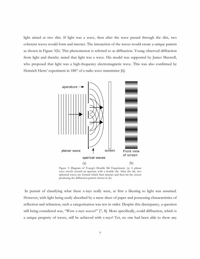
light aimed at two slits. If light was a wave, then after the wave passed through the slits, two

coherent waves would form and interact. The interaction of the waves would create a unique pattern

as shown in Figure 3(b). This phenomenon is referred to as diffraction. Young observed diffraction

from light and thereby stated that light was a wave. His model was supported by James Maxwell,

who proposed that light was a high-frequency electromagnetic wave. This was also confirmed by

Heinrich Hertz’ experiment in 1887 of a radio wave transmitter [6].

Figure 3: Diagram of Young’s Double Slit Experiment. (a) A planar wave travels toward an aperture with a double slit. After the slit, two spherical waves are formed which then interact and then hit the screen producing the diffraction pattern shown in (b).

In pursuit of classifying what these x-rays really were, at first a likening to light was assumed.

However, with light being easily absorbed by a mere sheet of paper and possessing characteristics of

reflection and refraction, such a categorization was not in order. Despite this discrepancy, a question

still being considered was, “Were x-rays waves?” [7, 8]. More specifically, could diffraction, which is

a unique property of waves, still be achieved with x-rays? Yet, no one had been able to show any

(a) (b)

8

evidence to support the idea. J.J. Thomson, in 1898, suggested that the x-rays were produced when

the cathode rays were stopped and thereby produced electric and magnetic disturbances, which he

referred to as pulses [7]. These pulses were believed to be thin and could produce effects similar to

that of light. The absence of diffraction could be explained by the thickness of the pulse. In

opposition to Thompson’s claims, W. H. Bragg proposed in 1907, based on the understanding of

the photoelectric effect, that “x-rays are a particle stream of neutral particles, or doublets of +

−

charge” [8]. His proposition became known as the neutral-pair theory, which was strongly argued

against by C.G. Barkla [9]. Barkla performed x-ray scattering experiments which he believed supported

the electromagnetic theory proposed by G. Stokes. J. Stark put forth a different conjecture in 1909

supposing that x-rays were photons of energy and momentum in order to explain the “spatial

anisotropy” of x-rays [10]. Nothing could be experimentally verified, but the search for evidence of

diffraction was not dissuaded. The next seventeen years following Röntgen’s discovery, for which he

received the first Nobel Prize in 1913, had scientists exploring this avenue.

1.1.3 X-Ray Diffraction

From the Helmholtz dispersion theory [10,11], it was determined that electromagnetic waves with

extremely short wavelengths neither are reflected nor refracted [10]. Based on the discovered

characteristics of x-rays it was then reasonable to conclude that x-rays had small wavelengths.

Experiments were performed by Röntgen, H. Haga, C.H. Wind, and Walter and Pohl using primarily

a double slit methodology. While none of the results were conclusive in relation to diffraction, it was

determined that, if diffraction occurred, the wavelength of x-rays must be on the order of 10−9 cm

or smaller [12]. In order to observe diffraction of x-rays, it was clear that smaller slits, of similar

order to the x-rays themselves, would be required. In 1912, P. P. Edwald asked Max von Laue for

advice in relation to lattice structures of crystals and electromagnetic waves. Laue, unversed in the

field of crystals, inquired of the spacing between atomic layers of crystals. Edwald’s response

informed Laue that the crystal plane might just be what was needed for diffraction grating for x-rays.

Laue enlisted W. Friedrich and P. Knipping to perform experimental tests to assess Laue’s

hypothesis. X-rays were allowed to pass through a copper sulfate crystal and then on to the

9

photographic plate directly opposite the x-ray source, as shown in Figure 4. The results of their test

are displayed in Figure 5 and reveal that x-ray diffraction (XRD) had finally been achieved. A similar

procedure was performed with powdered copper sulfate, but no comparable result was observed,

thus speaking to the value of the crystal for diffraction of x-rays. This also supported the notion that

x-rays were waves (although later quantum theory revealed that they can also be modeled as particles

very much like what Bragg had suggested in his pair-electron theory).

Figure 4: Diagram (a) and photograph (b) of the apparatus used to first observe x-ray diffraction. X-rays were produced in the chamber on the left which were then sent through a hole (Al) in a lead screen (S). The beam of x-rays then passed through four shutters (B1-B4) and finally through the crystal, which was surrounded by four photographic plates (P1-P4). A lead case (K) shielded the equipment. Figures taken from Ref. [13] and [10], respectively.

X-rays were then classified as waves, but the next task was to understand how they were produced.

Laue proposed that x-rays “contained only a number of discrete wavelengths and that these ones are

responsible for the spots” as can be seen in Figure 5 [10]. But it was W.H. Bragg’s son, W.L. Bragg,

who gave an accurate explanation. W. L. Bragg suggested that, unlike Laue’s idea, x-ray wavelengths

were indeed continuous. However, x-rays were being “reflected” by the lattice planes of the crystal

[10]. With equidistance between each crystal plane the spacing between the spots would be explained.

(a) (b)

10

W. L. Bragg’s theory, which later was named Bragg’s Law, relates the distance between crystal planes

to the angle of the x-ray inclination and the wavelength of the x-rays. Laue had experimented by

reflecting x-rays with copper sulfate and then a zinc sulfide crystal. Using his own equation, Bragg was

able to explain the diffraction patterns Laue observed [12]. In 1915 W. L. Bragg and his father received

the Nobel Prize for their work

.

Figure 5: Picture of the first x-ray diffraction achieved. (a) shows the results found when a crystal of copper sulfate was used while (b) is with powdered copper sulfate. Figure taken from Ref. [10].

1.1.4 XRD of Crystals

The achievement and explanation of x-ray diffraction opened the door for further understanding of

crystallography (the structure of crystals). W. L. Bragg stated, “The examination of crystal structure,

with the aid of x-rays [gave] for the first time an insight into the actual arrangement of the atoms in

solid bodies,” [12]. Specifically, the positioning of atoms impacts the external characteristics of the

crystal. However, there are several ways of arranging the atoms to produce the same outward structure.

The distinction between these different arrangements can be determined by how they react to x-rays

[14], which is done using x-ray diffraction.

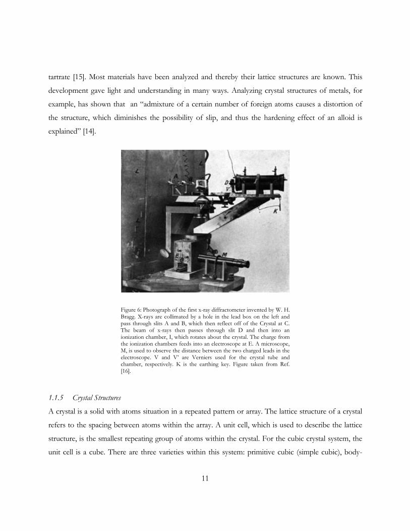
W. H. Bragg invented a new and improved machine, which more appropriately relayed information

regarding the arrangement and spacing of the lattice structure of crystals. This new apparatus (Figure

6) was the first x-ray diffractometer. Among the first materials analyzed by this machine were rock salt,

zinc blende, potassium ferrocyanide, potassium bichromate, quartz, calcite, and sodium ammonium

(a) (b)

11

tartrate [15]. Most materials have been analyzed and thereby their lattice structures are known. This

development gave light and understanding in many ways. Analyzing crystal structures of metals, for

example, has shown that an “admixture of a certain number of foreign atoms causes a distortion of

the structure, which diminishes the possibility of slip, and thus the hardening effect of an alloid is

explained” [14].

Figure 6: Photograph of the first x-ray diffractometer invented by W. H. Bragg. X-rays are collimated by a hole in the lead box on the left and pass through slits A and B, which then reflect off of the Crystal at C. The beam of x-rays then passes through slit D and then into an ionization chamber, I, which rotates about the crystal. The charge from the ionization chambers feeds into an electroscope at E. A microscope, M, is used to observe the distance between the two charged leads in the electroscope. V and V’ are Verniers used for the crystal tube and chamber, respectively. K is the earthing key. Figure taken from Ref. [16].

1.1.5 Crystal Structures

A crystal is a solid with atoms situation in a repeated pattern or array. The lattice structure of a crystal

refers to the spacing between atoms within the array. A unit cell, which is used to describe the lattice

structure, is the smallest repeating group of atoms within the crystal. For the cubic crystal system, the

unit cell is a cube. There are three varieties within this system: primitive cubic (simple cubic), body-

12

centered cubic (bcc), and face-centered cubic (fcc) which is also known as cubic close-packed. The

cubic crystal system is represented in Figure 7. Because fcc materials, such as copper, aluminum, gold,

and silver, are more easily malleable and altered, they are more commonly studied. Most materials are

polycrystalline, meaning they are made up of many different crystals. A single crystal, or crystallite,

within the material is called a grain.

Figure 7: Diagram of the cubic crystal system. The cubic crystal system is used to describe the lattice structures of the atoms that make up thin films. There are three types of structures, (a) primitive cubic (simple cubic), (b), body-centered cubic (bcc), and (c) face-centered cubic (fcc), which is also known as cubic close-packed.

1.1.6 Thin Films

Thin films are material substances with thicknesses typically on the order of nanometers and with a

length and width several orders of magnitude larger than their thickness. Their applications can vary

from semiconductors and microelectronics to optical lenses. The grains within the thin film material

are positioned at different angles in relation to the surface of the film, called the orientations of the

grain. Miller indices are used to define a crystal’s orientation by notating the normal vector of the

crystal plain that is parallel to the surface of the film. The number of orientations that a cubic structure

can be rotated to is infinite. However, in fcc materials only, a few are of high interest, namely the (111)

and (100) orientations for fcc crystals. Figure 8 demonstrates this concept.

(a) (b) (c)

13

Figure 8: Diagram of the (111) and (100) crystal planes. When the (111) plane of atoms (a) or the (100) plane of atoms (b) are parallel to the surface, the crystal is said to be in the (111) or (100) orientation, respectively.

The variance of orientations that are in a film is referred to as the film’s texture, and the formation and

alteration of such texture is of great interest [17-20]. The way a film is deposited as well as the substrate

chosen affect the resulting texture of the developed film. However, the texture can also be altered after

deposition. Applying heat to crystal grains causes them to grow. In the process of grain growth, the

overall texture of the film can change. This is called a texture transformation. The particulars and

determining factors of this outcome are not clearly understood [17-20]. To understand what causes

texture transformations requires significant analysis of the grain orientations that make up a thin film.

Such analysis is commonly performed by x-ray diffraction.

1.2 Recent XRD Experiments

While there are many different cubic structures of thin films, XRD research has focused primarily on

face-centered-cubic (FCC) metallic films [21,17-20], specifically on transformations from the (111) to

(100) orientation. Because atoms return or reside in the lowest energy state possible, XRD

experimentation has focused on the minimization of energy to help determine the influences driving

grain growth for specific orientations. Various elements that impact the energy are surfaces and

interfaces, grain boundaries, and stress [21-22]. The displacement from equilibrium divided by the total

length of the object is called strain energy. When stress is applied to atoms, it causes them to move,

(a) (b)

14

and thereby producing strain energy on the film. Strain energy can be modeled by Hooke’s law, which

in one-dimensional is given by the expression,

𝑈 =

1

2𝑘𝑥2, (1)

where 𝑈 is the energy, 𝑘 is a constant, and 𝑥 is the displacement from the equilibrium position. Atoms

form bonds in order to lower their energy state. To create two differing surfaces, those bonds are

broken, which increases the atoms’ energy. This is called surface and interface energy. Grain

boundaries are simply the barrier or interface between two different grains.

1.2.1 Carol and Thompson Model

A theory that many have held for a significant period of time [17-20] throughout the analysis of thin

films using XRD has been the Thompson and Carol model [21]. This model states that what drives the

texture transformation from one orientation to another is based on there being a competition between

the stress energy and surface and interface energy on thin films. In comparing the (111) and (100)

orientations, the former is preferred for minimization of surface energy while the latter is favored by

stress energy minimization. For thicker films, the ratio of surface area to volume is considerably small,

delegating the surface energy impact negligible. Therefore, this model states that the stress energy leads

to a transformation to (100) grains for thicker films. Conversely, thinner films have a much higher

ratio of surface to volume. Thus transformations ending in a strong (111) texture are expected for the

thinner films. Accordingly, it then follows that there would be a critical thickness, 𝑡𝑐, below which a

film should remain entirely of (111) oriented grains and above which it completely transforms to (100)

oriented grains after being annealed [23].

However, discrepancies have arisen with this model based on recent data analysis. A significant factor

that leads to the inaccuracy of the current model is that, despite variation in the duration of the

annealing process, data collection has not resulted in a clearly defined critical thickness [17]. Rather, a

gradual transition from one orientation to the other appears over a range of thicknesses, as shown in

Figure 9. One study has also observed a transformation occurring despite the thin film being removed

15

from the substrate, thus eliminating a prominent source of the proposed driving force for the

transformations [17]. Theoretical calculations have also shown that the stress is not big enough to

impact the observed transformations [17, 19-20].

Figure 9: Graph of XRD data. This graph gives the (111) fractional intensity vs. thickness of the thin film and reveals a gradual transition from the (111) to (100) orientation for a range of 400-600˚C samples instead of a sharp transition as proposed by the Thompson and Carol Model. Figure taken from Ref. [26].

1.2.2 Houghton College’s Research

To better understand what the driving force behind texture transformations is, Houghton College has

investigated how deposition rate and temperature affects the amount and speed of transformation [24,

25]. While progress has been made and the deposition rate and temperature do affect the

transformation, the full understanding and explanation for such occurrences have not been accounted

for. Thus, to further study and evaluate other factors and components involved in texture

transformation of thin films, Houghton College seeks to develop an x-ray diffractometer to perform

this significant research.

16

Chapter 2

THEORY

2.1 X-Ray Production

In a vacuum tube, x-rays are produced when a stream of electrons are accelerated towards a metal

target. Two different kinds of x-rays can be produced. When an electron interacts with an atom, one

possibility is that an incident electron is deflected by an atom of the target [27]. The electron loses

energy from the deflection, giving rise for it to emit a photon, which is referred to as a Bremsstrahlung

x-ray (Figure 10a). Bremsstrahlung x-rays have a roughly continuous spectrum of wavelengths. If, on

the other hand, an accelerating electron has enough energy, it can interact as before to emit a

Bremsstrahlung x-ray or it could knock out an electron from the target’s atoms. The latter occurrence

creates a hole in an inner orbital of the target’s atom. An electron from the atom’s upper shell will then

fall into the hole, which is at a lower energy state. To account for the reduction in energy of this

electron, an x-ray is emitted from the atom. This x-ray will have an energy and wavelength that is

characteristic to the difference from the outer to inner orbital, which is related to the material of the

target. Hence these types of x-rays are referred to as characteristic x-rays (Figure 10 b). Characteristic

x-rays from the same source have identical amplitude and frequency.

Figure 11 plots the intensity vs. wavelength of the Bremsstrahlung and characteristic x-rays. While

Bremsstrahlung x-rays have a higher intensity at lower wavelengths, characteristic x-rays have a higher

magnitude of intensity overall. The different peaks in Figure 12 represent the different intensities for

the corresponding outer shell from which an electron drops to fill in the hole created in an inner shell.

Characteristic x-rays occur at distinct wavelengths while Bremsstrahlung x-rays occur almost anywhere

and at significantly lower intensities, thereby forming background compared to characteristic x-rays.

Therefore, the x-rays used for analysis for x-ray diffraction are primarily characteristic x-rays.

17

Figure 10: Diagram of Bremsstrahlung and characteristic x-ray production. An incident electron interacts with atom in (a) and loses energy thereby emitting a Bremsstrahlung x-ray. Characteristic x-rays are demonstrated in (b) where the incident electron has enough energy to knock out an electron orbiting the atom. Electrons from the atom’s upper shells fall into the holes in the lower energy states. Again, the reduction of energy causes x-rays characteristic to the atom’s properties to be emitted.

Figure 11: Graph of an x-ray spectrum. This intensity vs. wavelength graph compares Bremsstrahlung and characteristic x-rays. Bremsstrahlung x-rays form background with its continuous spectrum while characteristic x-rays have a higher intensity forming peaks corresponding to the energy difference from the orbitals from which those x-rays were formed.

Incident electron

Electron with reduced energy

Emitted x-ray

Incident electron

Electron with reduced energy

Ejected electron

Emitted x-ray

(a) (b)

18

2.2 Wave Interference

X-rays are a type of electromagnetic wave. Waves can have different wavelengths, amplitude, and

frequency. The wavelength is the distance between successive maxima of the wave function, the

amplitude is the height of each maximum, and the frequency is the number of wavelengths that pass

by a given point in space per unit time. The interaction between waves is referred to as interference.

Mathematically the wave function is described as,

𝜓 = 𝐴𝑠𝑖𝑛(𝑘𝑥 − 𝜔𝑡 + 𝜙), (2)

where 𝐴 is the amplitude, 𝑘 =2𝜋

𝜆 is the wave number (and 𝜆 is the wavelength), 𝑥 is the position

vector, 𝜔 = 2𝜋𝑓 is the angular frequency (and 𝑓 is the frequency), 𝑡 is the time, and 𝜙 is the phase

shift from a reference point. When waves interact, their wave functions are added together. Consider

two nearly identical waves 𝜓1 = 𝐴𝑠𝑖𝑛(𝑘𝑥 − 𝜔𝑡) and 𝜓2 = 𝐴𝑠𝑖𝑛(𝑘𝑥 − 𝜔𝑡 + 𝜙), where 𝜓1 has

𝜙 = 0 such that 𝜓2has a phase shift in reference to 𝜓1. Then the interaction of 𝜓1and 𝜓2can be

described as,

𝜓1 + 𝜓2 = 𝐴𝑠𝑖𝑛(𝑘𝑥 − 𝜔𝑡) + 𝐴𝑠𝑖𝑛(𝑘𝑥 − 𝜔𝑡 + 𝜙)

= 2𝐴cos (−𝜙

2) 𝑠𝑖𝑛 {

1

2(2𝑘𝑥 − 2𝜔𝑡 + 𝜙)}

= 2𝐴 cos (

𝜙

2) 𝑠𝑖𝑛 (𝑘𝑥 − 𝜔𝑡 +

𝜙

2). (3)

Because 𝑐𝑜𝑠𝜙

2 is not dependent on 𝑡, the whole quantity 2𝐴cos [

𝜙

2] acts as the amplitude of the

resulting wave. Let Ν be the set of natural numbers. Then for all numbers 𝑛 𝜖 Ν, any values of

𝜙 = (2𝑛 + 1)𝜋 result in Equation 3 equaling zero. So when the phase difference between two waves

is an odd multiple of pi, often called “out of phase”, their interaction results is no wave. This result is

called destructive interference and is demonstrated in Figure 12.

19

Figure 12: Diagram of destructive interference. Destructive interference is the interaction of two waves that are completely out of phase, that is

𝜙 = (2𝑛 + 1)𝜋. Because the waves are offset such that when one wave is at its maximum amplitude the other is at its minimum, the waves cancel each other out.

Furthermore, for all 𝑛 𝜖 Ν, any values of 𝜙 = (2𝑛)𝜋 results in Equation 3 simplifying to

𝜓1 + 𝜓2 = 2𝐴𝑠𝑖𝑛(𝑘𝑥 − 𝜔𝑡 + 𝑛𝜋). (4)

Thus, when the phase difference between two waves is an even multiple of pi, called “in phase”, the

resulting wave has an amplitude twice that of individual waves’ amplitudes. This is called constructive

interference and is shown in Figure 13.

Figure 13: Diagram of constructive interference. Constructive interference occurs when two waves that are in phase, that is

𝜙 = (2𝑛 + 1)𝜋, with each other interact. The resulting wave has the combined amplitude of the two original waves’ amplitudes.

20

Destructive and constructive interference are the two extremes of wave interaction. However, if two

waves have a phase difference 2𝑛𝜋 < 𝜙 < (2𝑛 + 1)𝜋, then the resulting wave has an amplitude, 𝐴′,

of 0 < 𝐴′ < 2𝐴.

Given two waves that are in phase at the source, the phase difference, 𝜙, depends on the difference in

the paths of two waves, called the path length difference (𝑝. 𝑑. 𝑙) as given by

𝜙 =

2𝜋

𝜆(𝑝. 𝑑. 𝑙). (5)

When 𝑝. 𝑑. 𝑙 is an improper fraction of the wavelength, specifically when 𝑝. 𝑑. 𝑙 = (𝑛 +1

2)𝜆, then

Equation 5 simplifies to,

𝜙 = (2𝑛 + 1)𝜋. (6)

This result signifies that the x-rays are in destructive interference. On the other hand, if 𝑝. 𝑑. 𝑙 = 𝑛𝜆

then Equation 5 becomes

𝜙 = (2𝑛)𝜋, (7)

implying that the x-rays are in constructive interference. In other words, given that x-rays are in

constructive interference, it can be stated that the 𝑝. 𝑑. 𝑙 = 𝑛𝜆. The significance of this fact is

explained in the following section.

2.3 Bragg’s Law

X-ray diffraction uses principles given by Bragg’s law, which acts on the idea that the atoms of the

material form atomic planes [28]. Consider two beams of characteristic x-rays traveling in constructive

interference and parallel to each other toward the sample material at an angle 𝜃 from the surface of the

sample. It is shown in Figure 14 that the second beam of x-rays, which reflects off the second plane of

atoms, must travel an extra distance of 2𝑑𝑠𝑖𝑛𝜃 further than the first. In other words,

21

𝑝. 𝑑. 𝑙 = 2𝑑𝑠𝑖𝑛𝜃. Because constructive interference occurs when 𝑝. 𝑑. 𝑙 = 𝑛𝜆, Bragg’s Law, as given

by the following, concludes that in order to observe constructive interference with this setup then,

2𝑑𝑠𝑖𝑛𝜃 = 𝑛𝜆. (8)

Figure 14: Diagram demonstrating Bragg;s Law. Two beams of characteristic x-rays travel in constructive interference and parallel to

each other toward the sample material at an angle 𝜃. The second beam of X-rays that reflect off the second plane of atoms must travel an extra

distance of 2𝑑𝑠𝑖𝑛𝜃 than the first. In other words the 𝑝. 𝑑. 𝑙 = 2𝑑𝑠𝑖𝑛𝜃.

Given a known 𝜃, 𝜆, and 𝑛, the distance, 𝑑, between the planes can then be solved for. Because the

geometry of crystal structures are already known, from a measured 𝑑 the orientation of the crystals in a

film can be determined. With a specific 𝜆, only certain angles will satisfy this Bragg’s Law. Let 𝜃𝐵 be

the Bragg angle which satisfies Equation 8 for that sample, given a specified 𝜆. Because of the variance

of amplitudes a wave can have between it being in constructive and destructive interference, a range of

𝜃 values near 𝜃𝐵 will produce similar results when simply considering the two plane model in Figure

14. However, those results will have a lower intensity compared to those related to 𝜃𝐵 . Effectively, on

an intensity vs. theta plot this gives a broad based peak centered at 𝜃𝐵 . However, in reality there are a

𝜃 2𝜃 𝜃

22

large number of planes in the sample. Because of this, for every x-ray offset from 𝜃𝐵 there is a

corresponding x-ray reflecting off some lower plane that will destructively interfere. This reduces the

intensity around 𝜃𝐵 and thereby forms a sharp peak, as demonstrated in Figure 15, at 𝜃𝐵 due primarily

to constructive interference. Note that only characteristic x-rays are considered in this situation,

because Bremsstrahlung x-rays have a continuous spectrum of wavelengths, resulting in no angular

dependence of the amplitude of the outgoing wave.

Figure 15: Graph of counts vs. 2-Theta of data collected from XRD scan. This is a scan of a 1039nm film that was annealed at 100°C for one hour. There are two sharp peaks that appear at the Bragg angles for two orientations. This figure is taken from Ref. [29].

2.4 Intensity Fraction

X-rays are considered to have a particle-wave duality. This means that the wave function given by

Equation 2 can also be thought of as a probability function for the position of an x-ray. Results of

XRD scans display counts versus angle of inclination. If the angle meets the requirements as given

above for constructive interference, the probability of an x-ray traveling from the sample in that

direction is high, resulting in lots of counts. From past research, the angles at which constructive

interference occurs have already been identified for most materials. Accordingly, noting the angle at

which high numbers of counts occurs implies the orientation of the thin film. From these graphs the

proportion of the film that is 111 or 100 is determined from its area of the peak of the corresponding

23

crystal orientation in relation to the total area of both peaks. This is referred to as the intensity fraction.

The intensity fraction of the (111) orientation is given by

where 𝐴111 and 𝐴100 are the area underneath the peak that occurs at the corresponding angle for

(111) and (100) orientations, respectively. An analogous equation describes the intensity fraction for

the (100) orientation. These equations allow us to analyze collected data by producing data points,

which can be used to form graphs like Figure 9.

𝑓111 =

𝐴111

𝐴111 + 𝐴100, (9)

24

Chapter 3

APPARATUS

3.1 Introduction

The XRD machine at Houghton College is built upon a 6x4 ft table with an aluminum semicircle of

radius slightly less than 2 ft upon which two aluminum bars (called arms) with lengths 26.93 in and

27.06 in rotate by way of two Lin Engineering 101411 stepper motors. A sample is mounted on one of

the arms above the axis of rotation, while a detector is attached to the other arm. Both arms are

positioned and moved, using LabVIEW, to hold a theta-two theta relationship to each other. A

Philips-Norelco x-ray source is lined up on one side with the straight edge of the semicircle. The x-ray

source is powered by a HiTeck 40 kV, 25 mA variable power supply. Lead and steel shielding

surrounds the XRD as safety measures. The overall setup is shown in Figures 16-19.

Figure 16: Top view schematic of Houghton College’s XRD machine. The X-ray source, sample mount, detector, and motors are labeled

accordingly. X-rays hit the sample at an angle 𝜃 and reflect off the

sample at 2𝜃 from the X-rays’ original path.

X-Ray source

Motors

Detector

Sample mount

𝜃

𝜃 2𝜃

25

Figure 17: Topview photograph of Houghton College’s X-ray diffractometer. X-rays are collimated by a steel rod towards the sample mount, which rotates at a given velocity of a stepper motor. The detector rotates at two times the velocity of the sample mount. Steel shielding surrounds the entire apparatus as shown.

3.2 Mechanics

3.2.1 Stepper Motors

Two Lin Engineering 101411 stepper motors move across a 0.5 in thick semicircle. These motors are

designed such that the rotating cylinder shaft has a small slice removed along its entire length, thus

making it an imperfect round surface. To correct this, a sleeve with a wall thickness of 0.06 in was

secured onto the motor shaft by two 4-40 set screws as shown in Figure 20. An O-ring is placed onto

the sleeve between the set screws. The motors are positioned with the shaft horizontal to the

semicircle such that they rotate on the O-ring across the surface. Only 0.25 in of the shaft hangs over

the edge of the semicircle.

X-Ray source

Motors

Detector

Sample mount

Collimator

26

Figure 18: Side view schematic of XRD setup. The sample mount is attached to the sample arm which rotates via a stepper motors and an O-ring. The detector arm is set up in a similar manner.

Figure 19: Side view picture of Houghton College’s X-ray diffractometer. Bearing mounts allow the arms to rotate freely on the axis, and a gap between the two arms prevents unwanted friction.

Sample Mount

Motor

Bearing mounts

Sample Arm

Semicircle

Detector Arm Arm P

late

Set screws

O-ring

Motor

Sample Mount

Bearing mounts

Semicircle

O-ring

Detector Arm

Plate

27

Figure 20: Side view schematic (a) and picture (b) of the stepper motor. The motor shaft has a cylinder sleeve attached by two setscrews. An O-ring is placed between the setscrews.

The precision of the results taken by the XRD machine are affected by the diameter of rotating shaft.

With a smaller diameter, the motors can be positioned at set angles or travel desired distances more

accurately. With the sleeve added to the motor shaft, the outer radius of the O-ring is 0.15 in. Lin

Engineering 101411 stepper motors move at 400 steps/cycle, and the radius of the semicircle is 23.07

in. Thus, the precision these motors will produce is given by the following expression,

(

O − ring cycle

400 𝑠𝑡𝑒𝑝𝑠) (

0.15 semicircle cycle

23.07 O − ring cycle) (

360°

1 cycle) = 0.006

degrees

step. (10)

Knowing the precision of the apparatus helps to determine the accuracy of the results obtained from

the XRD machine.

3.2.2 Rotating Arms

The stepper motors rotate around the semicircle via two aluminum arms. They are connected to the

arms by a 0.25 in thick aluminum plate. The arms are 27.25 in long and, being secured by bearing

mounts, rotate about a 0.5 in shaft, called the axis, centered on a semicircle. There is a 0.125 in gap

Motor

Motor shaft

Cylinder sleeve

Set screw

Motor

Motor shaft

Cylinder sleeve

Set screw

O-ring

(a) (b)

r

28

between the two arms to avoid friction and hindrance to the arms movements. The two arms differ in

that the sample arm has a sample mount and the detector arm holds a Vernier DRM-BTD Digital

Radiation Monitor. The sample mount is secured to an 8x2x0.25 in (length by width by height) plate

which rests on a block attached to the arm in order to elevate the sample to be in line with the beam of

x-rays from the source. On the detector arm approximately 1ft. 9in. from the bearing mount, a student

radiation monitor is placed in a frame and attached to the arm. Besides the two arms, the only other

item on the axis is a 0.25 in. thick aluminum plate that simply acts as a cap to ensure the arms remain

on the axis at all times. The plate is secured to an aluminum block that is attached to the semicircle.

3.2.3 Shielding

The x-ray source is collimated by a steel rod that is placed flush against the source. The rod is 0.12 in

thick and has a diameter of 0.87 in and length of 25 in. The rod ends just short of the sample mount.

This causes radiation levels to be at background of 0.05 𝑚𝑅𝑒𝑚

ℎ𝑟 everywhere except directly in line with

the collimating rod. Lead blocks are stacked directly in line with the x-ray beam on the opposite end of

the source to reduce the high levels of radiation. Because everywhere else is at background, 0.125 in

thick steel panels surrounds the rest of the machine. There are eight panels all with a height of 18 in

attached via steel angles around the perimeter of the table that the source and semicircle are secured

onto. More steel angles and small rectangle pieces of steel connect the panels together and cover any

gaps to contain any stray radiation caused by reflection. The two panels closest to the axis are mounted

on hinges such that they fold down, allowing easy access to the machine. Three steel panels, two that

are 3x18 in and one that is 30 in by 6 ft, attached to a steel bar channel act as a roof to the steel box.

They are secured to the rest of the box via more steel angles. Figure 21 demonstrates this set up.

3.3 Software and Circuitry

3.3.1 Motor control system

The stepper motors are controlled by LabVIEW, a visual programming language, as shown in

Appendix A. The program operates based upon user inputs and constants defined from machine

29

specifications. From these conditions the speed of both motors, the total run time, and the number of

data points collected are determined.

Figure 21: Topview of shielding around Houghton College’s x-ray diffractometer. (a) Topview of shielding with the roof (b) removed. The hinges in (a) allow the those two panels to act as doors for easy access to the machine. Steel angles and rectangles are used to secure the side panels to each other and to the table.

The user specifies the target position (in steps) which determines where the motors should move to on

the semicircle. The acceleration, deceleration, and jerk of the motors are also inputted by the user.

These inputs affect how quickly the motor starts up and slows down, thereby impacting the

positioning of the motor given a set target position. The remaining inputs are 𝑡, the time taken to

collect each data point, and 𝑑 the number of data points taken per degree.

To perform the necessary calculations, LabVIEW requires 𝑁360, the number of steps it takes the

motors to travel a whole circle of radius, R. This quantity can be expressed given the ratio,

(a) (b)

30

𝑁360

𝑅=

400 𝑠𝑡𝑒𝑝𝑠

𝑟, (11)

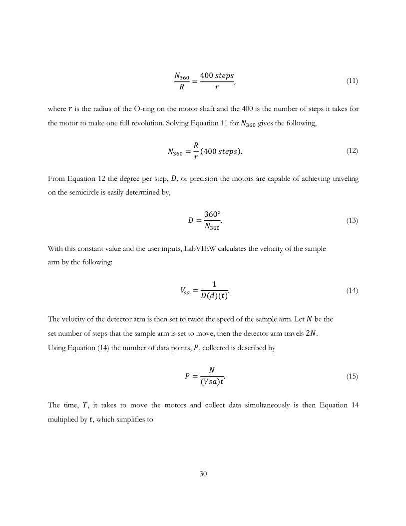
where 𝑟 is the radius of the O-ring on the motor shaft and the 400 is the number of steps it takes for

the motor to make one full revolution. Solving Equation 11 for 𝑁360 gives the following,

𝑁360 =

𝑅

𝑟(400 𝑠𝑡𝑒𝑝𝑠). (12)

From Equation 12 the degree per step, 𝐷, or precision the motors are capable of achieving traveling

on the semicircle is easily determined by,

𝐷 =

360°

𝑁360. (13)

With this constant value and the user inputs, LabVIEW calculates the velocity of the sample

arm by the following:

𝑉𝑠𝑎 =

1

𝐷(𝑑)(𝑡). (14)

The velocity of the detector arm is then set to twice the speed of the sample arm. Let 𝑁 be the

set number of steps that the sample arm is set to move, then the detector arm travels 2𝑁.

Using Equation (14) the number of data points, 𝑃, collected is described by

𝑃 =

𝑁

(𝑉𝑠𝑎)𝑡. (15)

The time, 𝑇, it takes to move the motors and collect data simultaneously is then Equation 14

multiplied by 𝑡, which simplifies to

31

𝑇 =

𝑁

𝑉𝑠𝑎. (16)

Knowing the time and number of data points collected allows the user to make adjustments to control

the parameters of the results.

Figure 22 displays the flow of information from the LabVIEW to the motor. When the program runs,

the information it generates is transferred to the NI Motion 8.1 driver, essentially transforming user

inputs into a readable form that the PCI 7344 card can interpret. Once the PCI 7344 card receives the

information it relays the commands to the MID 7602 power drive, which in turns sends the

appropriate signals to the motor leads.

Figure 22: Schematic of information flow from the user to the XRD. The user places inputs into the LabVIEW program which then sends the corresponding signals to the NI motion driver which eventually is sent to the two stepper motors causing them to move accordingly.

During each run the radiation monitor counts the number of x-rays detected at each angle. This is then

sent to the LabVIEW interface via a Vernier LabPro interface as Figure 23 demonstrates. The data

collected is then exported into a graph of counts vs. angle at the end of each run.

Figure 23: Depiction of X-ray counts fed back into the computer program. The number of x-rays detected at each angle is sent to LabVIEW via a LabPro interface.

LabVIEW NI Motion 8.1 PCI 7344 card

Motor

MID 7604/7602

Power drive

Motor

Student Radiation Monitor

LabPro LabVIEW

32

3.3.2 Power supply circuit

Figure 24 shows the circuit used to generate x-rays alongside an actual photograph of the

source. A DC 12 V power supply in series with a variable resister produces a current of

electrons that travel through the filament. Attached to the circuit is a 40 kV power supply that

is grounded on the positive terminal. A Cu target is also grounded, thereby creating a positive

40 kV potential difference from the filament to the target. Electrons are accelerated from the

filament toward the target by this potential difference. The interactions of the electrons with

the target then produce Bremsstrahlung and characteristic x-rays.

Figure 24: Schematic (a) of the x-ray producing circuit and (b) the actual source. In (a) a 40 kV power supply is attached to a DC and variable resister circuit. Electrons are accelerated toward the metal target by the potential difference from ground to the filament, thereby producing Bremsstrahlung and characteristic x-rays. For (b) the source has two leads connected to the Cu filament inside a vacuum tube (North American Philips Co: 32119).

8V

40kV

Filament

Cu target

Variable Resistor

Cu targets

33

Chapter 4

CONCLUSION

The X-ray diffractometer at Houghton College is mechanically complete. The x-ray source circuit is

complete and produces x-rays. The beam of x-rays has been collimated, leaving only a small area

exposed to more than background radiation of 0.05mRem

hr. Lead blocks have been set up to decrease

the higher levels of radiation, and steel shielding surrounds the entire diffractometer to lower radiation

levels from anything that reflects from the collimation x-rays. A LabVIEW program successfully

controls the movements, including distance, velocity, acceleration, and jerk, of two stepper motors

which in turns rotates the sample holder and detector to maintain the relationship required by Bragg’s

law.

While the main components of the machine are set up, some more adjustments are required before the

the X-ray diffractometer can be operated. A couple angle irons and a small rectangular panel of

shielding must be made to ensure full enclosure of x-rays during a test run. Furthermore, a wider hole

needs to be drilled to feed the cable of the detector through, and the radiation levels must be measured

near the whole outside of the steel box. The stepper motors are not consistent in the distance traveled

for a set number of steps, so adjustments need to be made to reduce the slipping and thereby increase

the accuracy of the machine. Also, the LabVIEW program must be edited to ensure that the data is

only collected while the motors are moving, and not long after they have reached their target position.

34

Appendix A

LABVIEW BLOCK DIAGRAMS

Figure 25: LabVIEW block diagram showing how information is used and controls the XRD. The user places inputs into the program, which then controls the motor movements.

35

Figure 26: LabVIEW block diagram continued from Figure 25. Based on user inputs from Figure 25, this diagram creates an array to store data from the detector. Data is then exported to an external file.

36

R e f e r e n c e s

[1] W. Crookes. Phil. Trans. R. Soc. Lond. 170, 135 (1879).

[2] W. Crookes, J. Franklin Inst. 108, 305 (1879).

[3] W. Röntgen, Science 3, 227 (1896).

[4] S.P. Thompson, Light : Visibile And Invisible. (MacMillan and Co.,London, 1912) p. 304.

[5] T. Young. Phi. Trans. R. Soc. Lond. 94, 1 (1804).

[6] R. A. Raymond, J. W. Jewett Jr. Physics for Scientists and Engineers with Modern Physics (Cenage

Learning, 2010) p. 987.

[7] W. Röntgen, G. Stokes, J. Thomson, Röntgen Rays, (Harper & Brothers, NY,

1898), 70.

[8] P. Ewald, Fifty Years Of X-Ray Diffraction, (Published for the Internation Union of

Crystallography by A. Ooosthoek’s Uitgeversmij, Utrecht, 1962) p. 13.

[9] R. H. Stuewer, Brit. J. Hist. Sci 5, 259 (1971)

[10] N. Robotti, Rend. Fis. Acc. Lincei, 24,7 (2013)

[11] H. Von Helmholtz, Ann Physik 48, 389, (1893).

[12] W.L. Bragg, Nobel Lecture, 228, 370 (1922).

[13] W. Friedrich, P. Knipping, M. Laue, Ann. Phys., 346, 979 (1913).

[14] W.L. Bragg, The Scientific Monthly, 20,117 (1925).

[15] W.H. Bragg, W.L. Bragg, Proc. R. Soc. Lond. A. 88, 430 (1913).

[16] W. H. Bragg, W. L. Bragg, X-Rays and Crystal Structure (G. Bell & Sons,1915), p. 145.

[17] J. Greiser, P. Mu¨ller, C.V. Thompson, E. Arzt. Scripta Mater 41 ,710 (1999).

[18] P. Sonnweber-Ribic, P. A. Gruber, G. Dehm, E. Arzt. Acta Mater 54, 3870 (2006).

[19] P. Sonnweber-Ribic, P.A. Gruber, G. Dehm, H.P. Strunk, E. Arzt. Acta Mater 60, 2397 (2012).

[20] J. Greiser, P. Mu¨ llner, E. Arzt. Acta Mater 49, 1041 (2001).

[21] C.V. Thompson, R.J. Carel. Mech. Phys. Solids. 44, 657 (1996).

37

[22] J. A. Floro, C. V. Thompson, R. Carel, P.D. Bristowe, J. Mater. Res. 9, 2411 (1994).

[23] C.V Thompson, R.J. Carel. Mech. Phys. Engin., B32, 215 (1995).

[24] B. Hoffman, J. Yuly, K. Flemington, P. Lashomb, SRI (Houghton College, NY, 2014

unpublished).

[25] K. Flemington, Undergraduate Thesis. Houghton College, NY, 2015 (unplublished).

[26] S. P. Baker, B. Hoffman, L. Timian, A. Silvernail, E. A. Ellis. Acta Mater 60, 7126 (2013).

[27] P. A. Tipler, R. A. Llewellyn. Modern Physics (W.H. Freeman and Company, NY,

1999) 145.

[28] W. L. Bragg. Proc. R. Soc. Lond. A. 89, 469 (1914).

[29] M. Kirkland, L. Vincett. SRI presentation (Houghton College, NY, 2015,

unpublished).