115

Design and characterization of a high voltage resistor divider at 60 Hz

Design and characterization of a high voltage resistor divider at 60 Hz

David J. Rincón1, Julio C. Chacón2, Gabriel Ordóñez3 1david.rincon1@correo.uis.edu.co, 2cchacon@uis.edu.co, 3gaby@uis.edu.co

Universidad Industrial de Santander Bucaramanga, Colombia

Artículo de investigación

Abstract

This chapter proposes a high voltage resistor divider design that minimizes the influence of the capacitive effects on the divider’s ratio due to its dimensions and position. Moreover, the proposed configuration enables a fast and accurate approximation of the capacitive effects, which in turn, makes feasible to estimate the ratio of the divider design by performing a simulation of its circuit model. A resistor divider prototype with the proposed design was constructed and compared with a Foster’s divider. The experimental estimation of the dividers ratios was performed by the sphere gaps test, according to the standard 4-IEEE-2013. The experimental results show that the constructed divider is three times less influenced by the capacitive effects than the Foster’s divider, without the need of a high voltage electrode. Moreover, a d ifference of -0,6% between the simulated and experimental ratios shows that the proposed technique to estimate the divider’s ratio is suitable for the proposed design, so it useful as a design tool.

Keywords: High-voltage techniques, Resistor divider, Voltage divider, Voltage measurement, Simulation. Resumen

En este artículo se propone un diseño sencillo de divisor resistivo de alta tensión que minimiza la influencia de los efectos capacitivos en la relación de tensión, basado en las dimensiones y la posición de sus elementos. Además, la configuración propuesta permite realizar una aproximación rápida y precisa de los efectos capacitivos, lo que a su vez permite estimar la relación del divisor por medio de una simulación de su modelo circuital. Un divisor prototipo con la configuración propuesta, fue construido y comparado un divisor Foster de alta tensión. La estimación experimental de la relación de los divisores se llevó a cabo mediante la prueba de sphere gaps, de acuerdo con lo establecido en el estándar 4-IEEE-2013. Los resultados muestran que el divisor construido esta tres veces menos influenciado por los efectos capacitivos que el divisor Foster, sin la necesidad de un electrodo de alta tensión. Además, una diferencia de -0,6% entre los valores de las relaciones simuladas y las experimentales muestran que la técnica para estimar la relación del divisor es adecuada para el diseño propuesto, lo cual resulta útil como herramienta de diseño.

Palabras clave: Técnicas de alta tensión, divisor resistivo, divisor de tensión, medición de tensión, simulación.

© 2017. IAI All rights reserved

Actas de Ingeniería Volumen 3, pp. 115-122, 2017

http://fundacioniai.org/actas

116

1. Introduction Selection of a high voltage divider is not a simple task;

there are different types with their advantages and disadvantages [1-3]. To decide what type of divider is the most appropriate, the most important criterion is to define the signal type and then determine if the divider accuracy is suitable for the measurement [4]. Usually, resistor dividers are not preferred to measure high ac voltages due to the influence of the temperature and the capacitive effects on the divider’s ratio. New technologies allow to manufacture resistors of GΩ with tolerances of 0,1% and temperature coefficients of 50 ppm\∘C. However, the traditional methods to solve the capacitance influence issue are expensive [2].

This chapter proposes a resistor divider design whose simple configuration facilitates the construction of the divider and minimizes the influence of the different capacitive effects on the divider ratio based only on the size and the position of the divider components. In addition, the characteristics of the design enables to perform a fast approximation of the capacitive effects to simulate the circuit model of the divider and estimate its ratio with reasonable accuracy. To evaluate the design performance, a prototype divider was constructed and compared with a Foster’s resistor divider with similar characteristics. Both dividers were characterized in theory and practice; the experimental estimation of the ratios was performed according to the procedure of chapter 14 of the standard 4-IEEE-2013 [6].

The results show that the constructed prototype is three times less influenced by the capacitive effects than the Foster’s divider. For the prototype, a difference of -0.6% between the estimate ratio with the distributed estimation approach and its experimental value was obtained, therefore the fast approximation of the capacitive effects and the simulation of its circuit model can be used as a design tool to estimate the ratio of a divider with the proposed design. This chapter is presented as follows: Section 2 describes the models used to characterize the dividers. In section 3 the characterization and the ratio estimation of the dividers are performed. In section 4, the experimental results are presented, analyzed and compared with the estimate ratios. Finally, the main conclusions are presented.

2. Theoretical Framework

Voltage dividers that are composed by passive

elements can be classified into three types: resistive, capacitive and mixed (damped capacitive). Each type has its advantages and disadvantages [2, 3, 5]. Due to the high resistance value and the influence of the capacitive effects, the voltage ratio of a resistor divider has a non-linear behavior against the signal frequency. For this reason, it is common to measure dc voltages with the resistive type. Nevertheless, in this paper a resistor divider is a viable alternative because the type of signal to be measured, 60 Hz (low frequency and steady state), as well as because of the low cost of its elements. In addition, the proposed design facilitates the construction of the divider.

2.1 High voltage resistor dividers characterization A conventional model of a resistor divider based on

distributed parameters is shown in Figure 1. It considers the three most significant capacitive effects, the self-capacitance effect of each resistor pC , the mutual

capacitance to ground potential eC and last the mutual

capacitance to the high voltage electrode hC .

Figure 1. Resistor divider model considering the most

significant capacitive effects [2]

At low frequency the inductive effects and pC are

neglected [1, 2]. eC and hC have opposite effects, in fact,

one of the ways to mitigate eC ’s effects is to place a stress

ring electrode on top of the divider in order to increase

hC ’s effects [2, 7]. Without this electrode hC is often

neglected. There are other techniques to mitigate eC ’s

effects such as shielding the resistors with a screen at a fixed potential [2, 5]. These techniques require a lot of resources and are difficult to implement.

For the theoretical analysis, the model of a resistor divider considering only capacitive effects to ground is

shown in Figure 2 [1]. aR is the High Voltage (HV)

resistor, bR is the Low Voltage (LV) resistor and vR is

the voltmeter resistor. The voltage ratio for this model is given by equation (1), where n is the aR ’s number of

segments, /ai aR R n for i=1,2,3,...,n and

( )( )eq b v b vR R R R R . The capacitive currents in each

branch are /Cek k CekI V Z for k=1, 2, 3, .. , n, b.

1aia CF b

eq

RV I V

R

(1)

Where:

1 2 3

1 2 3

( 1) ( 2) ...

...

a Ce Ce CenCF

a Ce Ce Cen Ceb

nI n I n I II

I I I I I

Solve CFI analytically would be a difficult task due to

the following:

1. As the number of branches n increase, the value of

ekC has a non-linearly decrease [8].

2. The parallel impedance on each branch CekZ

depends on the signal frequency and ekC ’s value;

1/Cek ekZ j C .

117

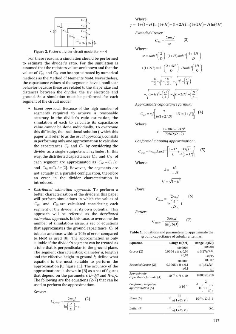
Figure 2. Foster’s divider circuit model for n = 4

For these reasons, a simulation should be performed to estimate the divider’s ratio. For the simulation is assumed that the resistors values are known and that the

values of ekC and hkC can be approximated by numerical

methods as the Method of Moments MoM. Nevertheless, the capacitance values of the segments have a nonlinear behavior because these are related to the shape, size and distances between the divider, the HV electrode and ground. So a simulation must be performed for each segment of the circuit model.

Usual approach. Because of the high number of segments required to achieve a reasonable accuracy in the divider's ratio estimation, the simulation of each to calculate its capacitance value cannot be done individually. To overcome this difficulty, the traditional solution ( which this paper will refer to as the usual approach), consists in performing only one approximation to calculate the capacitances eC and hC by considering the

divider as a single equipotencial cylinder. In this

way, the distributed capacitances ekC and hkC of

each segment are approximated as /ek eC C n

and /hk hC C n [2]. However, the segments are

not actually in a parallel configuration, therefore an error in the divider characterization is introduced.

Distributed estimation approach. To perform a better characterization of the dividers, this paper will perform simulations in which the values of

ekC and hkC are calculated considering each

segment of the divider at its own potential. This approach will be referred as the distributed estimation approach. In this case, to overcome the number of simulations issue, a set of equations that approximates the ground capacitance eC of

tubular antennas within a 10% of error compared to MoM is used [8]. The approximation is only suitable if the divider’s segment can be treated as a tube that is perpendicular to the ground plane. The segment characteristics: diameter d, length l and the effective height to ground h, define what equation is the most suitable to perform the approximation [8, figure 11]. The accuracy of the approximations is shown in [8] as a set of figures that depend on the parameters D=d/l and H=h/l. The following are the equations (2-7) that can be used to perform the approximation:

Grover:

02

2ln

Grover

lC

D

(2)

Where:

1 1 1 1 2ln ( )l 1n ln2 4( )H H H H H H

Extended Grover:

02Ex

lC

(3)

Where:

1 12 4 4(1 )

Hsinh H sinh

D D

1 12 4 4(1 2 )

H HH sinh Hsinh

D D

2 2

212 2 4

D D DH

2 2

2 2(1 ) (1 2 )4 4

D DH H

Approximate capacitance formula:

0

74 ln 1

(1 2 / )AcfC l D

ln D

(4)

Where: 21 30 124

70 ( 2)

D D

HD D

Conformal mapping approximation:

41

0

1 ' '4

4 1 'Cma

k k kC dcosh

k k

(5)

Where:

1

Hk

H

2' 1k k

Howe:

02

4ln 1

Howe

lC

D

(6)

Butler:

02

ln 16Butler

dC

D

(7)

Table 1. Equations and parameters to approximate the ground capacitance of tubular antennas

Equation Range H(h/l) Range D(d/l)

Grover (2) ≤0,0004

0,0004 ≤ H ≤ 0,04 ≥0,04

≤0,008 ,, H 0 250 27

≤0,35

Extended Grover (3) ≤0,0005

0,0005 ≤ H ≤ 0,1 ≥0,1

≤0,007

, H0 33

≤1 Approximate capacitance formula (4) H 410 10 0,003≤D≤10

Conformal mapping approximation (5)

410 lnH

2

31

Howe (6) ln / D

35

1 2 D 310 1

Butler (7) ln / D

35

1 2 ≫1

118

Table 1 shows the range of the parameters H and D for the different equations. Equations (6) and (7) are expressions for the free space capacitance of thin and thick tubes [8]. This is the minimum capacitance value that can be obtained for a segment of the circuit model. Moreover, the accuracy of the free space expressions is within 2% against MoM for 0,15 ≤ D ≥ 1 , therefore these values are desirable to perform the simulations in order to improve the results accuracy [9, 10]. The maximum error for these expressions is around 4% for D≃0,25. 3. Proposed design 3.1 Characteristics

The design consists of a series configuration of axial resistors that hangs down from the HV conductor and must be perpendicular to the ground to improve the

accuracy in eC ’s approximation. The outer electrical

insulation between the resistors is the air, therefore a maximum gradient of 5 kV/cm must be ensured to avoid surface flashovers and discharges [1, 7, 11]. The gradient is calculated as follows (equation 8).

VE

L

(8)

Where E is the voltage gradient, ΔV is the voltage drop in the resistor and L is the length of the resistor’s insulated part. To minimize the influence of capacitive effects on the proposed design the following conditions must be ensured:

The height of aR ’s lowest resistor should be high

enough to minimize eC ’s effects. In other words,

the parameter H=h/l must ensure that the

capacitance ekC will be approximated to its free

space value.

To neglect hC ’s effects, a minimum distance of 70

cm from aR ’s highest resistor to the HV conductor

is needed.

The capacity of the design depends on the HV conductor height and the characteristics of the resistors that are used. Therefore the following statements must be considerated during the design of the divider:

The length of the resistors is defined by its nominal voltage. So aR ’s length will depend on the

voltage level (peak value) to be measured.

Due to the characteristics of the design, the length

of aR is restricted by the HV conductor height and

the required distances to satisfy the minimization of the capacitive effects.

The influence of the capacitive effects on the divider ratio depends on the resistance value of

aR , so it should be as low as possible. However,

this value is limited by the power capacity of the resistors and the rms voltage level to be measured.

Weight of axial resistors should not be a trouble due to the series configuration.

3.2 Design highlights

Due to its characteristics the proposed design presents the following benefits:

1. The simplicity of the design facilitates the construction of the divider.

2. The capacitive effects are reduced overall based only on the divider dimensions and aR ’s distance

to ground and to the HV electrode.

3. Its configuration enables a fast and accurate approximation of the capacitive effects which is useful to estimate the divider’s ratio by a simulation of its circuit model.

4. It is a portable design.

These features make the design a simple and feasible option to perform ac HV measurements. Moreover, the design is ideal to be used as a reference system device due to its portable character.

4. Development and implementation of the proposal

First, the characteristics of each divider are presented, followed by the simulation of its circuit model in OrCAD to perform the voltage ratio estimation. The simulation only considers eC ’s effects (Figure 2),

because these can be approximated using the proposed equations in [8]. Finally, an experimental estimation of the dividers ratios was performed according to the procedure of chapter 14 of the standard 4-IEEE-2013 [6].

4.1 Foster’s high voltage divider

Characteristics. The laboratory’s ac Foster module, see Figure 3, includes a transformer and a high voltage resistor divider. The divider consists of four nominal resistors of 75 ± 10% MΩ, submerged in insulating oil, which form a HV

resistor aR =300 MΩ. The laboratory’s guide

mentions that the LV resistor is a set of resistors

whose final value is bR = 350 ± 2% kΩ. Due to its

age and the normal wear of the equipment, a change in the voltage ratio of the divider was detected. The HV and LV resistors of the divider were characterized, respectively, an insulation tester Fluke 1550C and a Fluke 105 Scopemeter were used. The measures indicate a change in the HV resistor with 'aR = 364 ± 5% MΩ, the LV

resistor remained as bR = 350 ± 0,6% kΩ.

Figure 3. Foster’s high voltage module. Transformer

parameters: power 20 kVA, frequency 60 Hz, PV =500 V and

SV =300 kV

119

Ratio estimation. Foster’s divider has a diameter of d=7 cm, a length of l=1,88 m and it is 1 cm above the ground plane. Two simulations with the distributed estimation approach and a number of segments n = 4 and n = 15 were performed. The parameters of the simulations are shown in Tables 2 and 3.

Table 2. Simulation Paramet. for the Foster’s divider for n=4

Parameter Value

aV 100 kVrms

f 60 Hz Rai’∴ i=1,2,3,4 91±5% MΩ

bR 350±0,6% kΩ

vR 10±1% MΩ

2eC (2) 12,37±1% pF

3eC (2) 12,73±1% pF

4eC (4) 18,1±2% pF

bC 200 pF

Table 3. Simulation Paramet. for the Foster’s divider for n=15

Parameter Value

aV 100 kVrms

f 60 Hz Rai’∴ i=1,2,3,4 24,27±5% MΩ

bR 350±0,6% kΩ

vR 10±1% MΩ

'eiC ∴ i=1,2,3,4 (3) (7) ±2% pF

'eiC ∴ i= 5,6,…,14 (3) ±1,5% pF

15eC (4) 10,28±0,7% pF

bC 200 pF

The simulations results and the resistive ratio for the Foster’s divider are shown in Table 4.

Table 4. Simulations Results for the Foster’s Divider

Effect of eC n Ratio

X – 1077±59 √ 4 1459±123 √ 15 1833±188

√ Parameter take into account - X Parameter not take into account

The results indicated that the ratio of the Foster’s

divider is heavily influenced by eC ’s effects. Due to the

fact that the circuit model is based on distributed parameters, the estimated ratio for n = 15 should be a better approximation. Nevertheless, the experimental ratio for the Foster’s divider should be lower than the

estimated ratios because hC ’s effects have a large

influence on the divider’s ratio due to the HV electrode size and its proximity to the divider, see Figure 3.

4.2 Constructed divider

In order to check the proposed design performance a prototype divider was constructed (see Figure 4). Since the divider’s diameter is quite small compared to its length on the right side of the figure an enlarged image of the HV resistors is shown. In the same way, on the left

side of the figure an enlarged image of the LV resistors is shown.

Figure 4. Constructed divider. On the left, 2 of 4 bR ’s

resistors. On the right, 3 of 30 aR ’s resistors

To bond the resistors, their wires were coiled and welded using tin. The wires were coiled to improve the mechanical stability of the divider and the tin was used to prevent the edge effect and to reinforce the resistors bond. A length of 2 cm for the resistor’s bond was chosen to maintain a suitable heat transfer to the outside [1, 11, 12].

Characteristics. Based on the characteristics of the

Foster’s divider and the available resistors: maxV ,

power, size, etc. a HV resistor aR = 300 MΩ and a

LV resistor bR = 350 kΩ were chosen. aR consists

of 30 resistors type HVR37 from Vishay BCcomponents and bR consists of 4 resistor type

100 Series from Riedon, whose aggregated cost was ≈ 15 USD. The resistors characteristics are shown in Table 5.

Table 5. Resistors characteristics for the constructed divider

1R 2R 3R

Resistance MΩ 10 0,1 0,05 Tolerance % 1 0,01 0,01 Maximum DC Voltage V 3500 250 250 Power W 0,5 0,25 0,25 Temperature Coefficient ppm / C 200 10 10

Usually, the temperature coefficient of the resistors should match to avoid non-linearity issues; in the prototype this is compensated by the high precision of

bR ’s resistors.

Ratio estimation. A uniform diameter d = 2,5 mm

was assumed for the constructed divider. aR ’s

length is l=0,92 m, its lowest resistor is around 1,2 m from the ground and the highest is at 70 cm from the HV conductor. Due to the characteristics of the proposed design, it is possible to assume

that only eC ’s effects must be considered in the

ratio estimation. The assumption that the resistor and their bound can be considered as tubes was done. Two sets of simulations were performed, on the first one eiC was approximated with the usual

approach /ei eC C n . On the second one eiC was

approximated with the distributed estimation

120

approach. For each set of simulations the ratio of the constructed divider was estimated for a number of segments n = 15, 30, 60. The parameters for the usual approach simulations are shown in Table 6; eC was approximated by (2).

Table 6. Simulations Parameters for the Constructed Divider

with /ei eC C n

Parameter Value

n = 15 n = 30 n = 60

aV 75 kVrms

f 60 Hz

aiR i=1,2,..,n 20±1% MΩ 10±1% MΩ 5±1% MΩ

bR 350±0,01% kΩ

vR 10±1% MΩ

/ei eC C n i=1,2,..,n 544±1% fF 272±1% fF 136±1% fF

bC 200 pF

The parameters for the simulations with the

distributed estimation approach are shown in Table 7. The free space capacitance expression for thin tubes (6)

was used to approximate eiC for n = 15, 30, 60.

Table 7. Simulations Parameters for the Constructed Divider with the distributed estimation

Parameter Value

n = 15 n = 30 n = 60

aV 75 kVrms

f 60 Hz

aiR i=1,2,..,n 20±1% MΩ 10±1% MΩ 5±1% MΩ

bR 350±0,01% kΩ

vR 10±1% MΩ

eiC i=1,2,..,n 936±1% fF 581±2% fF 383±1% fF

bC 200 pF

The results of the simulations for the constructed divider are shown in Table 8. The estimated ratios with the usual approach are equal for n = 15, 30, 60. On the other hand, the obtained values with the distributed estimation approach depend on n. In both cases, the results indicated that the constructed divider is sligthly influenced by the capacitive effects with a maximum difference of 3,77% between its resistive ratio and the estimated ratios.

Table 8. Simulation Results for the Constructed Divider

Effect of eC Ratio

X 888,1±9,4

/ei eC C n n = 15 n = 30 n = 60

892,7±9,1 892,7±9,1 892,6±9,1

eiC n = 15 n = 30 n = 60

902,0±9,5 908,0±9,9 921,5±10,5

4.3 Experimental ratio estimation

According to the standard 4-IEEE-2013, an alternating voltage measurement system must be able to measure the peak or the rms value of the test voltage. It establishes that an approved ac measurement system must have an overall uncertainty no longer than ±3% and a reference ac measurement system must have an overall

uncertainty no longer than ±1%. The concept of reference measurement system was introduced with the aim of improving the quality of high-voltage measurements, the idea is to avoid self-calibration in the laboratories [2]. In this way, the standard establishes that the calibration of a reference system is done by comparing its performance against a suitable standard measuring system with overall uncertainty traceable through national or international comparisons [6]. In the ac high voltage measurement, a standard measuring system will be referred at the end to a sphere gaps test that has been validated. However, due to the fact that this test was the main method of calibration for decades, most of the laboratories have the equipment to perform it [2]. For this reason and to avoid self-calibration, the standard establishes an untraceable sphere gaps test as an approved measure system. The last statement ensures that an untraceable sphere gaps test will not have the status of standard or reference system. The status of reference system is important because the standard allows to use it to calibrate approved systems based on the fact that reference systems guarantee the traceability and the low uncertainty of the measurement. In other words, the standard prohibits performing self-calibrations with untraceable sphere gaps tests, but the test by itself continues to be the standard for the ac high voltage measurements.

This paper conducts a type test to evaluate the performance of the proposed design, therefore a sphere gaps test performed as it is established in chapter 14 of the standard is a suitable option to validate (not to calibrate, due to the absence of traceability) the design. The sphere gaps from Haefely have a diameter of 25 cm. The test consists in applying a potential difference that is increased until a disruptive discharge occurs between the spheres. The peak value of the disruptive discharge voltage depends on the diameter and the distance S between the spheres, in addition to the environmental conditions. Chapter 14 of the standard includes: the

standardized disruptive discharge voltages dV , the

environmental conditions correction factor and a complete description of the test [6]. A sketch of the experimental setup is shown in Figure 5. The Foster’s transformer, the high voltage divider and the sphere gaps, with the protective resistor Rd=1 MΩ, are in a parallel configuration; the voltmeter is connected in

parallel with bR .

Figure 4. Experimental set up of the sphere gaps test

The rectified disruptive discharge voltage cV is

obtained applying correction (9) to the standardized

voltage dV according to: the atmospheric pressure ATP

121

mm Hg, the absolute humidity AH 3/g m and the

temperature T ∘C of the place where the test is performed [6].

0

0

273

273

1 0,002 8,5

c dV k V

tb

b t

hk

(9)

With 0 20t C , 0 760b mm Hg.

Foster’s divider experimental ratio. In the

measurement, a 105 Scopemeter from Fluke was used. The tester resistance with the 10:1 input connection is 10 MΩ. The measures of the environmental conditions are made with a Humidity/Barometer/Temp. meter model PHB-318 from Lutron Electronic. The test disruptive discharge voltages and the environmental conditions for the Foster’s divider are shown in

Table 9. VcU is the uncertainty of cV for a

confidence level of 95% with a coverage factor k = 2,13.

Table 9. Disruptive Discharge Voltage and Environmental Conditions for The Foster’s Divider

S mm

dV

kV

T

C

ATP mm Hg

AH

/ 3g m cV

kV

VcU

±

10 31,7 25,9 678,1 16,8 28,3 24,2 210

12 37,4 27,5 675,8 18,1 33,2 26,9 210

14 42,9 25,2 679,3 15,7 38,4 29,9 210

16 48,1 27,8 679,3 16,9 42,8 32,5 210

18 53,5 25,2 679,2 16,2 47,9 35,7 210

22 64,5 27,1 677,8 17,6 57,5 41,6 210

28 81,0 27,6 676,2 18,3 72,0 50,9 210

The standard establishes that at least ten

measurements must be performed for each disruptive discharge voltage, the measure is approved if the

standard deviation 1%std The measurements, its std

and the obtained ratios for the Foster’s divider are shown in Table 10. VMU is the uncertainty of voltmeter

measurements for a confidence level of 95% with k = 2,09.

Table 10. Foster’s Divider Measurements

S mm CV kV MproV V std % VMU ± Ratio

10 28,3 23,9 0,59 15,3 210 1185

12 33,2 27,9 0,86 28,9 210 1192

14 38,4 32,1 0,73 28,7 210 1195

16 42,8 36,2 0,17 24,5 210 1181

18 47,9 40,1 0,26 25,1 210 1194

22 57,5 48,6 0,42 27,7 210 1181

28 72,0 60,9 0,82 58,6 210 1182

Constructed Divider Experimental Ratio. The test

disruptive discharge voltages and the

environmental conditions for the constructed divider are shown in Table 11. VcU has a k = 2,13

for a confidence level of 95%.

Table 11. Disruptive Discharge Voltage and Environmental Conditions for the Constructed Divider

S mm dV kV T C ATP mm Hg AH / 3g m cV kV VcU ±

10 31,7 27,1 676,3 16,9 28,1 24,1 210

12 37,4 26,7 676,1 16,8 33,2 26,9 210

14 42,9 27,1 676,0 17,3 38,1 29,7 210

16 48,1 27,1 675,9 16,7 42,7 32,5 210

18 53,5 27,1 675,8 17,2 47,5 35,4 210

22 64,5 26,9 678,5 15,3 57,3 41,6 210

28 81,0 27,1 678,5 17,3 72,2 51,1 210

The measurements, its std and the obtained ratios

for the constructed divider are shown in Table 12. VMU

has a k = 2,08 for a confidence level of 95%.

Table 12. Constructed Divider Measurements

S mm

CV

kV

MproV

V

std

%

VMU

± Ratio

10 28,1 30,6 0,73 28,1 210 920,8

12 33,2 36,4 0,96 33,2 210 911,9

14 38,1 41,4 0,67 30,1 210 921,3

16 42,7 46,7 0,70 32,2 210 913,8

18 47,5 52,0 0,43 50,2 210 914,0

22 57,3 62,8 0,47 51,8 210 912,7

28 72,2 78,8 0,44 53,1 210 916,9

5. Results

The dividers mean ratio and its std deviation are

shown in Table 13. RU is the uncertainty of the

experimental ratios for a level of confidence of 95% with k = 2,03 for the Foster’s divider and k = 2,03 for the constructed divider.

Table 13. Overall Results

Divider Ratio std % RU ±

Foster’s 1187 0,53 15 Constructed 916 0,42 11

The estimated ratios on the Foster’s divider simulations have a minimum difference of -22,87% compared with its experimental value, this was expected

because hC ’s effects have a large influence on the divider

ratio and these were not considered in the simulations. The experimental ratio for the constructed divider exhibits a difference of 3,14% compared with its resistive ratio, three times less than the difference obtained for the Forster’s divider without the need of a HV electrode. Therefore the proposed design accomplishes the goal of minimizing the influence of the capacitive effects based only in the position and the size of the divider components. Also, a difference of -2,5% was found between the estimated ratios with the usual approach and its experimental value. On the other hand, a difference of -0,6% is obtained for the distributed estimation approach for n = 60. This result indicates that

122

the distributed estimation approach describes better the divider behavior than the usual approach because it considers each segment of the model at its own potential. For the constructed divider, a difference of -0,6% between the estimates is expected. Even so, a maximum difference of -2,2% for a confidence level of 95% can be obtained due to the experimental and the simulation uncertainties of 1,2% and 1,15%, respectively. Nevertheless, the fact that a difference of 2,2% is obtained from two independent estimates, increases the reliability on the estimated values.

6. Discussion

Based on the results, it is feasible to use another

resistors configuration with different characteristics to measure higher voltages. For example: 5 resistors MOX970 of 50 MΩ from OHMITE can be used to construct a divider up to 150 kVrms. Using a LV resistor of 300 kΩ from Vishay BCcomponents the divider resistive ratio is 860 and the estimated ratio with the proposed technique is 911. The resistors characteristics are shown in Table 14. In this case, the minimum height of the high voltage conductor required for the proposed design is 2,9 m.

Table 14. Resistors characteristics for a proposed divider

970MOXR 150R

Resistance MΩ 50 0,15 Tolerance % 0,5 0,01 Maximum DC Voltage V 60000 500

Power W 19,4 0,75

Temperature Coefficient ppm / C 50 50

7. Conclusions

A HV resistor design with a simple but effective

configuration was proposed. Not only does the configuration facilitate the construction of the divider, but also the experimental results indicate that it minimizes the influence of the capacitive effects on the divider’s ratio. In addition, the characteristics of the proposed design enable to make a fast and accurate approximation of the capacitive effects, which in turn, allows to estimate the divider’s ratio by performing the

simulation of its circuit model. In the case of the constructed prototype, the experimental ratio exhibits a difference of 3,14% compared with its resistive ratio, three times less than the difference obtained for the Forster’s divider, without the need of a HV electrode. Also, a difference of -2,5% between the estimated ratios with the usual approach and the experimental value was obtained. On the other hand, a difference of -0,6% is obtained with the distributed estimation approach for n = 60.

References [1] Naidu, M. & Kamaraju, V. (1995). High Voltage

Engineering second edition. USA: McGraw-Hill. [2] Kuffel, E., Zaengl, W. & Kuffel, J. (2000) High Voltage

Engineering Fundamentals Second edition. UK: Newnes. [3] Schwab, A. & Pagel, J. (1972). Precision capacitive voltage

divider for impulse voltagge measurements. IEEE Transactions on Power Apparatus and Systems 91, pp. 2376–2382.

[4] Harada, T. et al. (1976). Development of a high voltage universal divider. IEEE Transactions on Power Apparatus and Systems 95, pp. 595–602.

[5] Begamudre, R. (2006). Extra High Voltage ac Transmission Engineering (third edition). New York: New age international publisher.

[6] IEEE (2013). IEEE Standard for High-Voltage Testing Techniques.

[7] Pan, Y. et al. (2015). Development of 300-kv air-insulation standard impulse measurement system. IEEE Transactions on Instrumentation and Measurement 64, pp. 1627–1635.

[8] Rivera, D. et al. (1995). Approximate Capacitance Formulas for Electrically Small Tubular Monopole Antennas. USA: Naval Undersea Warfare Center Division.

[9] Butler, C. (1980). Capacitance of a finitelength conducting cylindrical tube. Journal of Applied Physics 51(11).

[10] Scharstein, R. (2007). Capacitance of a tube. Journal of Electrostatics 65(1), pp. 21-29.

[11] Ziegler, N. (1970). Dual highly stable 150-kv divider. IEEE Transactions on Instrumentation and Measurement 19, pp. 281–285.

[12] Pattarakijkul, D., Kurupakorn, C. & Charoensook, A. (2010). Construction and evaluation of 100 kv dc high voltage divider. In CPEM 2010, pp. 677–679.