DESIGN AND ANALYSIS OF TUBULAR …etd.lib.metu.edu.tr/upload/12619241/index.pdfI hereby declare that...

DESIGN AND ANALYSIS OF TUBULAR PHOTOBIOREACTORS FOR

BIOHYDROGEN PRODUCTION

A THESIS SUBMITTED TO

THE GRADUATE SCHOOL OF NATURAL AND APPLIED SCIENCES

OF

MIDDLE EAST TECHNICAL UNIVERSITY

BY

EMINE KAYAHAN

IN THE PARTIAL FULFILLMENT OF THE REQUIREMENTS

FOR

THE DEGREE OF MASTER OF SCIENCE

IN

DEPARTMENT OF CHEMICAL ENGINEERING

SEPTEMBER 2015

Approval of the thesis:



submitted by EMİNE KAYAHAN in the partial fulfillment of the requirements for

the degree of Master of Science in Chemical Engineering Department, Middle

East Technical University by,

Prof. Dr. Gülbin Dural Ünver

Dean, Graduate School of Natural and Applied Sciences

Prof. Dr. Halil Kalıpçılar

Head of Department, Chemical Engineering

Prof. Dr. İnci Eroğlu

Supervisor, Chemical Engineering Dept, METU

Asst. Prof. Dr. Harun Koku

Co-supervisor, Chemical Engineering Dept, METU

Examining Committee Members:

Prof. Dr. Ufuk Gündüz

Department of Biological, METU

Prof. Dr. İnci Eroğlu

Chemical Engineering Dept, METU

Asst. Prof. Dr. Harun Koku


Assoc. Prof. Dr. Serkan Kıncal


Assoc. Prof. Dr. Başar Uyar

Chemical Engineering Dept., Kocaeli University

Date: 01.09.2014

iv

I hereby declare that all information in this document has been obtained and

presented in accordance with academic rules and ethical conduct. I also declare

that as required by these rules and conduct, I have fully cited and referenced all

material and results that are not original to this work.

Name, Last Name: Emine Kayahan

Signature :

v

ABSTRACT



Kayahan, Emine

M.S., Department of Chemical Engineering

Supervisor : Prof. Dr. İnci Eroğlu

Co-supervisor : Asst. Prof. Dr. Harun Koku

September 2015, 195 pages

Hydrogen can be produced sustainably by utilizing organic wastes through

photofermentation. In order to obtain an economically feasible operation, the

photobioreactor design is of crucial importance. An optimal photobioreactor design

should provide uniform velocity and light distribution, low pressure drop, low gas

permeability and efficient gas-liquid separation. The aim of this study was to design a

pilot-scale photobioreactor satisfying these criteria and to test the reactor under

outdoor conditions with purple non sulphur bacteria. A glass, stacked tubular

bioreactor aimed at satisfying these criteria has been designed for outdoor

photofermentative hydrogen production. The design consists of 4 stacked U-tubes and

2 vertical manifolds. The hydrodynamics of the 3-dimensional model of this reactor

was solved via COMSOL Multiphysics 4.1. Two reactors, whose volumes were 9 and

11 L, were constructed based on the dimensions obtained by the model. A reactor was

constructed based on the dimensions obtained by the model. The reactor was operated

with recirculation of culture containing Rhodobacter capsulatus YO3 (hup-). Every

morning 10% of the culture was replaced by fresh feed. Experiments were lasted 10-

vi

20 days. When molasses was used as the carbon source under outdoor conditions, the

highest hydrogen productivity was found as 0.311 mol H2/(m3.h). Another parallel

reactor working with acetic acid which was also run in July 2015, the highest

productivity was found as 0.114 mol H2/(m3.h). Compared to nearly horizontal tubular

reactors, the glass stacked tubular reactor design results in less ground area and longer

life time.

Keywords: Photofermentation, manifold model, photobioreactor design,

biohydrogen, Rhodobacter capsulatus

vii

ÖZ

BİYOLOJİK HİDROJEN ÜRETİMİ İÇİN BORUSAL

FOTOBİYOREAKTÖRLERİN DİZAYNI VE ANALİZİ

Kayahan, Emine

Yüksek Lisans, Kimya Mühendisliği Bölümü

Tez Yöneticisi : Prof. Dr. İnci Eroğlu

Ortak Tez Yöneticisi : Yrd. Doç. Dr. Harun Koku

Eylül 2015, 195 sayfa

Hidrojen, fotofermentaston ile organik atıkları kullanarak sürdürülebilir bir şekilde

üretilebilir. Ekonomik bir üretim elde edebilmek için fotobiyoreaktör dizaynı son

derece önemlidir. Optimum fotobiyoreaktör tasarımında, homojen bir akış ve ışık

dağılımı, düşük basınç farkı, düşük gaz geçirgenliği ve verimli çalışan bir gaz-sıvı

ayırma ünitesi olmalıdır. Bu çalışmanın amacı, bu kriterleri sağlayacak pilot-ölçekli

bir fotobiyoreaktör tasarımı yapmak ve reaktörü mor sülfürsüz bakteri kullanarak açık

havada test etmektir. Açık havada fotofermentaston ile hidrojen üretimi amacını

taşıyan ve bu kriterleri sağlayacak, bir cam, borusal biyoreaktör tasarlanmıştır. Dizayn

4 adet U-tüpü, ve 2 adet dikey manifolddan oluşmaktadır. Bu reaktörün hidrodinamiği

3 boyutlu olarak COMSOL Multiphysics 4.4 kullanılarak çözülmüştür. Boyutları

model sonuçlarına dayandırılan 9 ve 11 L hacme sahip iki reaktör kurulmuştur. Reaktör

Rhodobacter capsulatus YO3 (hup-) suş kültürü devirdaim ettirilerek çalıştırılmıştır.

Her sabah reaktörlerden %10 kültür alınmış ve yerine besiyeri verilmiştir. Deneyler

10-20 gün sürmüştür. Açık havada yapılan deneyde, karbon kaynağı olarak melas

kullanıldığı zaman en yüksek hidrojen üretim hızı 0.311 mol H2/(m3.sa) olarak

viii

bulunmuştur. Temmuz 2015’te gerçekleştirilen paralel bir deneyde asetik asit ile içeren

besiyeriyle elde edilen en yüksek üretim hızı 0.114 mol H2/(m3.sa) dir. Dikey borusal

cam reaktör, hafif eğimli yatay plastik borusal reaktörlere göre daha az alan kaplar ve

daha uzun ömre sahiptir.

Anahtar Kelimeler: Fotofermentasyon, manifold modeli, fotobioyoreaktör tasarımı,

biyohidrojen, Rhodobacter capulatus

ix

To my family,

x

ACKNOWLEDGEMENTS

I would like to express my sincere gratitude to my supervisor, Prof. Dr. İnci Eroğlu.

Her guidance, advice, support and kindness gave me motivation during my thesis. I

would like to thank to my co-supervisor Asst. Prof. Dr. Harun Koku for his suggestions

and valuable contributions on my thesis. I also thank to Prof. Dr. Ufuk Gündüz and

Prof. Dr. Meral Yücel for their recommendations on biological systems.

I am indebted to Dominic Deo Androga for valuable comments, discussions, and help.

With the light of the information I gained while working with Dominic, I was able to

carry out my experiments. I also would like to acknowledge Emrah Sağır with his help

especially on working with bacteria. I would like to thank Dr. Siamak Alipour about

his contributions during the construction of the reactors. I am very happy having

worked with such friends.

I am thankful to chemical engineering student, Yağmur Özdemir, with whom I worked

on the light intensity distribution and absorption of molasses. I special thanks go to

Nihal Bayaki, Onurcan Arslan and Efe Seyyal. Their help in the pump selection, and

the development of a method for HPLC analysis was very valuable for me.

I would like to thank to the technical assistant Gülten Orakçı for her help in HPLC

analysis. I also would like to thank İsa Çağlar, Süleyman N. Kuşhan and Adil Demir,

who work in the Chemical Engineering Workshop.

xi

I would like to express my gratitude to Gökçe Avcıoğlu. Her friendship and advices

on the large scale operations gave me motivation during my studies. I am grateful to

Ezgi Yavuzyılmaz, Necip Berker Üner and C. Güvenç Oğulgönen for their support,

friendship and priceless brainstorming on chemical engineering topics. I also would

like to thank Barış Erdoğan who gave motivation and encouragement to me during my

thesis with his invaluable comments and guidance. I also would like to thank Esen

Özcan, Barış Özcan and Bilgi Alver for their friendship and support.

I would like to thank to my family for their invaluable support, love and faith in me. I

especially thank to my sister, Nagehan Kayahan for her precious friendship and

support not just only in this thesis but also in my whole life. I also thank to my mother,

father and grandfather. Their endless love and support gave me encouragement in

throughout my thesis.

I thank to Kazım Yılmaz and Ayhan İldam who work in İldam Cam for their help and

suggestions on the glass reactor.

This study was a part of the ongoing project funded by TÜBİTAK (114M436) and by

the METU BAP project (BAP-07-02-2014-007-538).

xii

TABLE OF CONTENTS

ABSTRACT ................................................................................................................. v

ÖZ…………………………………………………………………………………...vii

TABLE OF CONTENTS .......................................................................................... xii

LIST OF TABLES ..................................................................................................... xv

LIST OF FIGURES ................................................................................................. xvii

LIST OF SYMBOLS ............................................................................................. xxiii

LIST OF ABBREVIATIONS .................................................................................. xxv

CHAPTERS

1. INTRODUCTION .................................................................................................... 1

2. LITERATURE SURVEY ........................................................................................ 7

2.1 Hydrogen as an Energy Carrier .......................................................................... 7

2.2 Commercial Hydrogen Production Techniques ............................................ 8

2.2.1 Natural Gas Steam Reforming .................................................................... 8

2.2.2 Partial Oxidation of Hydrocarbons ............................................................. 9

2.2.3 Coal Gasification ......................................................................................... 9

2.2.4 Biomass Gasification ............................................................................ 10

2.2.5 Electrolysis ........................................................................................... 10

2.3 Review of Biohydrogen Production Technologies ...................................... 10

2.3.1 Photolysis ............................................................................................. 12

2.3.2 Dark Fermentation ................................................................................ 13

2.3.3 Photofermentation ................................................................................ 21

2.3.4 Integrated Systems ............................................................................... 33

2.3.5 Mixed Cultures for Simultaneous Dark and Photofermentation .......... 35

2.4 Photobioreactors for Hydrogen Production ................................................. 39

2.4.1 Panel Photobioreactors ......................................................................... 39

2.4.2 Tubular Photobioreactors ..................................................................... 41

2.5 Flow Distribution in Manifolds ................................................................... 44

3. STACKED U-TUBE PHOTOBIOREACTOR DESIGN ...................................... 53

xiii

3.1 Design Strategy ........................................................................................... 53

3.1.1 Reactor Selection ................................................................................. 53

3.1.2 Method of Attack ................................................................................. 57

3.2 Methods ....................................................................................................... 58

3.3. Mesh Convergence Study ............................................................................... 63

3.3 Effect of Design Parameters on Velocity and Pressure Distribution .......... 69

3.4 Evaluation and Final Selection .................................................................... 74

4. CONSTRUCTION AND OPERATION ............................................................... 77

4.1 Materials and Methods ................................................................................ 77

4.1.1 The Bacterial Strain.............................................................................. 77

4.1.2 Culture Media....................................................................................... 77

4.1.3. Analyses ............................................................................................... 79

4.2 Construction ................................................................................................ 82

4.2.1 Inlet and Outlet Manifolds ................................................................... 83

4.2.2 Tubing .................................................................................................. 84

4.2.3 Stand ..................................................................................................... 86

4.3 Pump Selection ............................................................................................ 86

4.4 Process Flow Diagram ................................................................................. 89

4.5 Operation ..................................................................................................... 90

4.5.1 Sterilization and Leakage Test ............................................................. 90

4.5.2 Inoculation............................................................................................ 90

4.5.3 Continuous Feeding ............................................................................. 91

4.5.4 Sampling .............................................................................................. 94

5. RESULTS AND DISCUSSION ............................................................................ 95

5.1 September 2014 Outdoor Experiment with Rhodobacter capsulatus YO3

(hup-) on Molasses (Run 092014) .......................................................................... 95

5.2 July 2015 Outdoor Experiments with Rhodobacter capsulatus YO3 (hup-)

(Run 072015) ....................................................................................................... 101

5.2.1 Run 072015-R1: Outdoor Experiment with Rhodobacter capsulatus YO3

(hup-) on Artificial Medium ............................................................................. 102


(hup-) on Molasses in July ............................................................................... 107

xiv

5.3 Overall Evaluation of the Stacked U-tube Reactor and the Comparison of

Productivities with Other Outdoor Studies .......................................................... 115

6.CONCLUSIONS AND RECOMMENDATIONS................................................ 121

REFERENCES ......................................................................................................... 125

APPENDICES

A. COMPOSITION OF THE GROWTH MEDIA .................................................. 137

B. MOLASSES ANALYSES .................................................................................. 139

C. DIAMETER SELECTION .................................................................................. 143

C.1. Light Intensity Measurements ...................................................................... 143

C.2. Photon Count Measurements ........................................................................ 145

C.3. Absorbance Experiments .............................................................................. 147

D. PUMP SELECTION ........................................................................................... 149

D.1. Experimental Procedure for Pump Selection ............................................... 149

D.2. pH variation .................................................................................................. 150

D.3. Experimental Data of the Pump Selection ................................................... 151

E. CALIBRATION CURVE OF THE DRY CELL WEIGHT ................................ 153

F. LIGHT ABSORPTION SPECTRA OF Rhodobacter capsulatus YO3 (hup-) ..... 155

G. SAMPLE GAS CHROMATOGRAM FOR GAS ANALYSIS .......................... 157

H. SAMPLE HPLC CHROMATOGRAM AND CALIBRATION CURVES OF

ORGANIC ACIDS AND SUCROSE ...................................................................... 159

I. MODEL OUTPUTS ............................................................................................. 163

J. OUTDOOR EXPERIMENTAL DATA ............................................................... 165

K. SAMPLE CALCULATION ................................................................................ 193

K.1 Sample Calculation for Productivity ............................................................. 193

K.2 Sample Calculation for Substrate Conversion Efficiency ............................. 194

K.3 Sample Calculation for Light Conversion Efficiency ................................... 194

xv

LIST OF TABLES

TABLES

Table 2.1: The comparison of dark fermentation studies in terms of their productivities

and substrate conversion efficiencies ......................................................................... 18

Table 2.2: The comparison of indoor photofermentation studies in terms of their

productivities and substrate conversion efficiencies .................................................. 27

Table 2.3: Comparison of productivities and yields for mixed cultures for simultaneous

dark and photofermentation ....................................................................................... 37

Table 3.1: The default values of Newton’s method…………………………………..62

Table 3.2: Details of runs done for the mesh convergence study. The volumetric flow

rate was 25 L/h (Ret=92), the tube pitch was 10.5 cm and the tube length was 1.4 m.

.................................................................................................................................... 66

Table 3.3: Results of mesh convergence study .......................................................... 68

Table 3.4: The summary of the parameters studied and corresponding non-uniformity

parameter. ................................................................................................................... 74

Table 5.1: The feeding strategy……………………………………………………...99

Table 5.2: The experimental results of hydrogen in outdoors with R. capsulatus YO3

on artificial medium under non-sterile conditions (RUN072015-R1). .................... 106

Table 5.3: The experimental results of hydrogen production outdoors with R.

capsulatus YO3 on molasses (RUN072015-R2) ....................................................... 113

Table 5.4: Summary of the results of experimental results ...................................... 116

Table 5.5: The comparison of outdoor studies in terms of productivities and substate

conversion efficiencies ............................................................................................. 117

Table D.1: The daily temperature and light intensity change………………………151

xvi

Table D.2: OD, and pH values for peristaltic and centrifugal pump ....................... 152

Table J.1: Daily variation in pH and cell concentration of RUN 092014. The

experiment started on September 10, 2014…………………………………………165

Table J.2: Daily variation in organic acid and sucrose concentration of RUN 092014.

The experiment started on July 10, 2014. ................................................................ 166

Table J.3: Daily variation in cell concentration of RUN 072015-R1. The experiment

started on July 12, 2015. ........................................................................................... 167

Table J. 4: Daily variation in pH of RUN 072015-R1. The experiment started on July

12, 2015. ................................................................................................................... 168

Table J.5: Daily variation in organic acid concentrations of RUN 072015-R1. The

experiment started on July 12, 2015. ........................................................................ 169

Table J. 6: Biogas production of RUN 072015-R1. The experiment started on July 12,

2015. ......................................................................................................................... 170


started on July 12, 2015. ........................................................................................... 171

Table J.8: Daily variation in pH of RUN 072015-R2. The experiment started on July

12, 2015. ................................................................................................................... 172

Table J. 9: Daily variation in organic acid and sucrose concentrations of RUN 072015-

R2. The experiment started on July 12, 2015. .......................................................... 173

Table J.10: Biogas production of RUN 072015-R2. The experiment started on July 12,

2015. ......................................................................................................................... 174

Table J.11: Data taken from the weather station on July 21, 2015. ......................... 174

Table J.12: Temperature data taken on July 21, 2015. ............................................. 185

xvii

LIST OF FIGURES

FIGURES

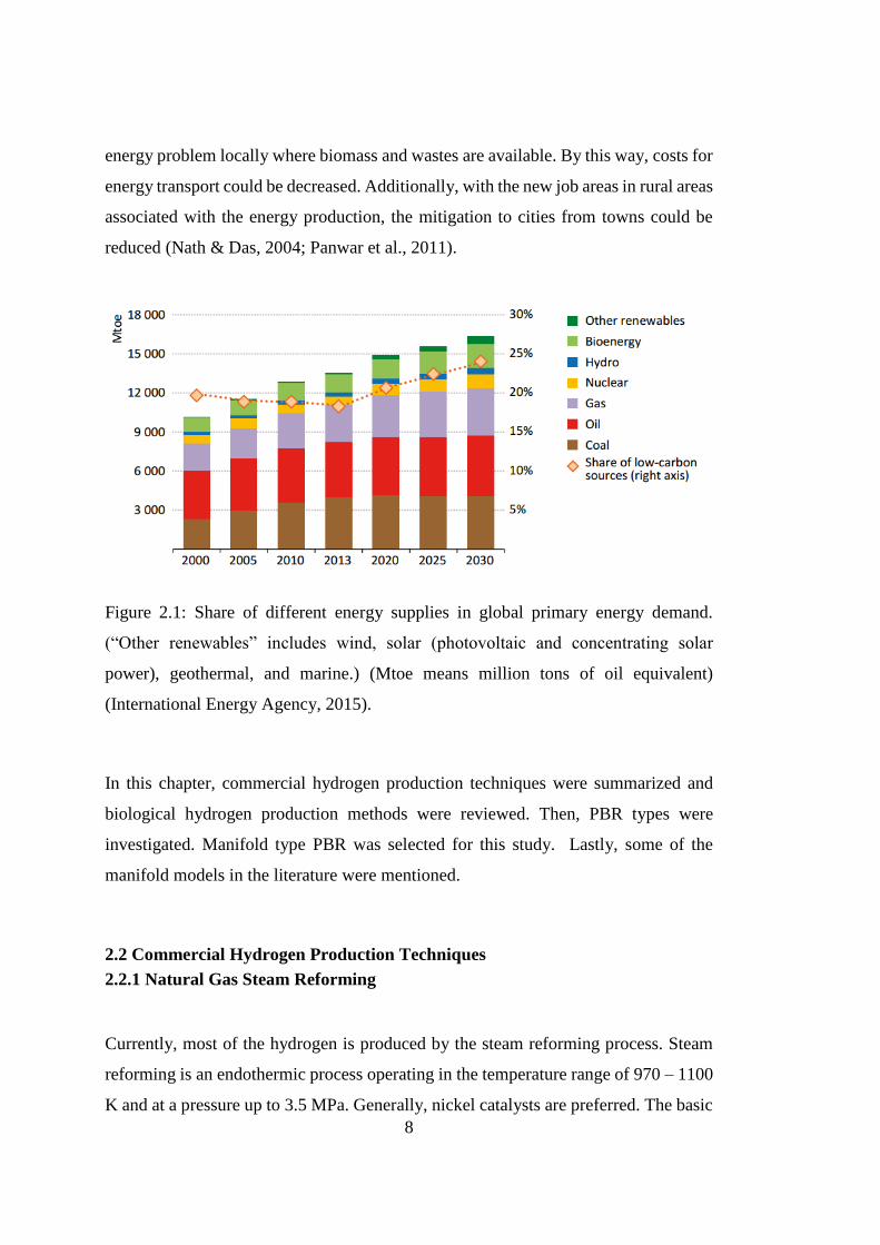
Figure 2.1: Share of different energy supplies in global primary energy demand.

(“Other renewables” includes wind, solar (photovoltaic and concentrating solar

power), geothermal, and marine.) (Mtoe means million tons of oil equivalent)

(International Energy Agency, 2015). .......................................................................... 8

Figure 2.2: Microbial bioenergy: Pathways for hydrogen production in dark

fermentation. .............................................................................................................. 15

Figure 2.3: Chronological summary of hydrogen productivities in dark fermentation

studies. ........................................................................................................................ 17

Figure 2.4: Hydrogen production pathway by photofermentation in PNSB (Androga,

Özgür, Eroglu, et al., 2012). ....................................................................................... 23

Figure 2.5: Chronological summary of hydrogen productivities in photofermentation

studies ......................................................................................................................... 24

Figure 2.6: Comparison of productivities of photofermentation ............................... 24

Figure 2.7: Cost items for two-stage biological H2 production ................................. 34

Figure 2.8: Breakdown of capital costs for two-stage biological H2 production ....... 34

Figure 2.9: Operating costs for photofermentation .................................................... 34

Figure 2.10: Chronological summary of hydrogen productivities in mixed cultures for

simultaneous dark and photofermentation ................................................................. 36

Figure 2.11: Panel type PBRs (4 L) operated in outdoor conditions with internal

cooling ........................................................................................................................ 40

Figure 2.12: Various types of tubular PBRs (Dasgupta et al., 2010) ......................... 42

Figure 2.13: Nearly horizontal tubular PBR (90 L) operated with Rhodobacter

capsulatus (Boran et al., 2012b). ................................................................................ 43

xviii

Figure 2.14: Velocity distribution of a manifold type PBR. The yellow streamlines

indicate the distribution of particle trajectory (Androga, 2014). ................................ 43

Figure 2.15: Flow distribution among the tubes of a manifold a type PBR (Androga,

2014) ........................................................................................................................... 44

Figure 2.16: (a) U type manifolds (b) Z type manifolds ............................................ 45

Figure 2.17:Domain discretization (a) higher level discretization in T-junctions (b)

lower level discretization in the tubes (Ablanque et al., 2010) .................................. 47

Figure 3.1: The stacked U-tube PBR geometry solved via COMSOL Multiphysics 4.4.

The tube pitch is 10.5 and the tube length is 4.0 m………………………………….63

Figure 3.2: Twenty meshes distributed around the manifolds (Distribution 1). ........ 64

Figure 3.3: Twenty meshes distributed around the inlet and outlet pipes (Distribution

2). ................................................................................................................................ 64

Figure 3.4: Twenty meshes were distributed along the inlet pipe (Distribution 3). ... 65

Figure 3.5: Twenty meshes were distributed around the tubes (Distribution 4). ....... 65

Figure 3.6: Effect of tube length on the fractional volumetric flow rate for a volumetric

flow rate of 25.0 L/h (Ret=92) and tube pitch 10.5 cm .............................................. 71

Figure 3.7: Effect of tube pitch for a volumetric flow rate of 25.0 L/h and a tube length

of 1.4 m ...................................................................................................................... 72

Figure 3.8: Effect of fractional volumetric flow rates for tube pitch and tube lengths of

10.5 and 1.4 m, respectively. ...................................................................................... 73

Figure 3.9: Pressure drop with respect to volumetric flow rate. The tube pitch and

lengths are 10.5 cm and 1.4 m. ................................................................................... 73

Figure 4.1: Inlet and Outlet manifolds (a) front view (b) side view…………………..84

Figure 4.2: a) U – tubes b) Tees for sampling and thermocouples ............................ 85

Figure 4.3: U-tube PBRs operated with an aquarium pump (left) and a peristaltic pump

(right). The experiment started on December 28, 2014 and lasted 3 days. ................ 87

Figure 4.4: Variation in cell concentration for different pump types for the first day.

The experiment started on December 28, 2014. ......................................................... 88

Figure 4.5: Variation in cell concentration for different pump types for 3 days. The

experiment started on December 28, 2014. ................................................................ 88

xix

Figure 4.6: Process flow diagram of the stacked U-tube PBR. T1 – T12 are the

temperature probes. V1 and V2 are check valves (1/3 psi), V4, V5, V6 and V7 are ball

valves. CW-in and CW-out are cooling water inlet and outlet, respectively. ............ 90

Figure 4.7: A photograph of the experimental set up (RUN 091025). The experiment

performed with R. capsulatus YO3 on molasses. ........................................................ 91

Figure 4.8: Side views of the Reactor 1. Experiment performed with R. capsulatus YO3

on acetic acid (RUN 072015 – R1) ............................................................................ 92


on molasses (RUN 072015 – R2). ............................................................................. 93

Figure 4.10: The parallel reactors run in July 2015. (RUN 072015-R1 and RUN

072015-R2). ............................................................................................................... 94

Figure 5.1: (a) Comparison of temperature variation with time for different tubes on

the 6th day of the experiment (T1, T5 and T9 were measured from the entrance,

midpoint and exit ports in tube 4, respectively) (b) Comparison of temperatures along

the length of the PBR on the 6th day of the experiment. The experiment started on

September 9, 2014. (T9, T10, T11 and T12 were measured from the exit ports of tube

4, tube 3, tube 2 and tube 1, respectively.)…………………………………………...96

Figure 5.2: (a) Comparison of temperature change along the length of the PBR on the

10th day of the experiment. (T1, T5 and T9 were measured from the entrance, midpoint

and exit ports in tube 4, respectively.) (b) Comparison of temperature change for

different tubes on the 10th day of the experiment. Experiment started on September 9,

2014. (T9, T10, T11, T12 were measured from the exit ports of tube 4, tube 3, tube 2

and tube 1, respectively.) ........................................................................................... 97

Figure 5.3: Relation between the temperature change and the daily solar radiation for

RUN072015-R1. T9 is measured from the exit port of the tube 4. Experiment started

on September 9, 2014. ................................................................................................ 98

Figure 5.4: Organic acid and pH variation in the reactor. Experiment started on

September 9, 2014. ................................................................................................... 100

Figure 5.5: Daily sucrose concentration change. Daily sucrose concentration change.

Experiment started on September 9, 2014. .............................................................. 100

xx

Figure 5.6: Daily cell concentration change. Experiment started on September 9, 2014.

.................................................................................................................................. 101




the length of the PBR (RUN072015-R1) on the 9th day of the experiment. Experiment

started on July 12, 2015. (T9, T10, T11, T12 were measured from the exit ports of tube

4, tube 3, tube 2 and tube 1, respectively.) ............................................................... 103


RUN072015-R1. T9 is measured from the exit port of the tube 4. The experiment was

started on July 12, 2015. ........................................................................................... 104

Figure 5.9: (a) Variation in cell concentration (b) Daily hydrogen production in

outdoors with R. capsulatus YO3 on artificial medium under non-sterile conditions

(RUN072015-R1). .................................................................................................... 105

Figure 5.10: Variation in pH and organic acid concentration in outdoors with R.

Capsulatus YO3 on artificial medium under non-sterile conditions (RUN072015-R1).

The starting date of the experiment was 12.07.2015. Feeding started on the 4th day.

.................................................................................................................................. 107


RUN072015-R2. T4 and T12 were measured from after the distribution manifold and

before the combination manifold, respectively. Both of them were on the Tube 1.

Experiment started on July 12, 2015. ....................................................................... 109

Figure 5.12: The comparison of the temperatures for RUN072015-R1 and

RUN072015-R2. R1-T12 and R2-T12 were measured on the Tube 1 just before the

combination manifold. Experiments started on July 12, 2015. ................................ 109

Figure 5.13: Daily variation in sucrose concentration for RUN 072915-R2. The initial

sucrose concentration was 5 mM (data not shown). The starting date of the experiment

was July 12, 2015. .................................................................................................... 110


capsulatus YO3 on molasses (RUN072015-R2). The starting date of the experiment

was 12.07.2015. Feeding started on the 5th day. ..................................................... 110

xxi

Figure 5.15: Cell concentration and hydrogen production in outdoors with R.

Capsulatus YO3 on molasses (RUN072015-R2). The starting date of the experiment

was 12.07.2015. ....................................................................................................... 112

Figure 5.16: Daily hydrogen productivity. The starting date of the experiment was

12.07.2015. ............................................................................................................... 112

Figure 5.17: Mol fractions of carbon dioxide, carbonate and bicarbonate with respect

to pH. ........................................................................................................................ 114

Figure C.1: Light intensity variations at different depths according to different sucrose

concentrations. Compartments were filled with pure sucrose at different

concentrations ……………………………………………………………………...144


concentrations. The compartments were filled with diluted molasses containing

different amounts of sucrose. ................................................................................... 144

Figure C.3: Light intensity variation for 3 cm depth according to different sucrose


different amounts of sucrose. ................................................................................... 145

Figure C.4: Schematic representation of the spectroradiometer .............................. 145

Figure C.5: Photon counts with respect to wavelength for 19 mM sucrose containing

molasses at different thicknesses ............................................................................. 146

Figure C.6: Photon counts with respect to wavelength for different concentrations of

sucrose in molasses. ................................................................................................. 147

Figure C.7: Comparison of absorbance values for different molasses dilutions ..... 148

Figure D.1: pH variation for different pump types for the first day. The starting date

of the experiment was Decemeber 12, 2014………………………………………..150

Figure D.2: pH variation for different pump types for the first day. The starting date

of the experiment was Decemeber 12, 2014. ........................................................... 150

Figure E.1: Calibration curve for the dry cell weight versus OD660 of the Rhodobacter

capsulatus YO3 (hup-) (Öztürk, 2005). Optical density of 1.0 at 660 nm corresponds to

0.4656 gdcw/Lc……………………………………………………………………..153

xxii

Figure F.1: Light absroption spectra of Rhodobacter capsulatus YO3 (hup-). Optical

density at 660 nm was 1.4…………………………………………………………..155

Figure G.1: A sample gas chromotogram (Androga, 2009)…………………….......157

Figure H.1: A sample HPLC chromotogram. (Androga, 2009). Retention times of

lactic, formic, acetic, propionic and butyric acid are 22.0, 24.5, 26.5, 31.3 and 38.6

min, respectively…………………………………………………………………...159

Figure H.2: HPLC calibration for lactic acid ........................................................... 160

Figure H.3: HPLC calibration for formic acid ......................................................... 160

Figure H.4: HPLC calibration for acetic acid .......................................................... 160

Figure H.5: HPLC calibration for propionic acid .................................................... 161

Figure H.6: HPLC calibration for butyric acid ........................................................ 161

Figure I.1: Velocity profile for 3.8 m tube length, 10.5 cm tube spacing and 25 L/h

volumetric flow rate………………………………………………………………..163

Figure I.2: Pressure profile for 3.8 m tube length, 10.5 cm tube spacing and 25 L/h

volumetric flow rate. ................................................................................................ 163

xxiii

LIST OF SYMBOLS

ad Ratio of the diameter to length in the

distribution manifolds ___

ac Ratio of the diameter to length in the

combination manifolds ___

Cp Specific heat capacity at constant pressure J/(kg.K)

F Volume force vector N/m3

F0 Friction in the straight tube section ___

I Light intensity W/m2

I Identity tensor ___

M Ratio of all the port areas to the manifold area ___

of the manifold

M0 Momentum flow at the entrance ___

n Boundary normal unit vector pointing

out of the domain ___

N Number of channels ___

p Pressure Pa

pout Outlet pressure Pa

q Heat flux vector W/m2

Q̇ Heat sources W/m3

xxiv

Q0 Total volumetric flow rate m3/s

Qi Flow rate of the ith channel m3/s

Rep Reynolds in the pipes of the manifold __

s Spacing between the tubes m

S Strain – rate tensor __

tH2 Duration of the hydrogen production process h

T Absolute temperature K

u Velocity vector m/s

uwall Velocity at the solid boundary m/s

VH2 Volume of the produced hydrogen L

Greek Letters

β Dimensionless volumetric flow rate ___

ζ Average total head loss coefficient for port flow ___

η Percent light conversion efficiency ___

μ Dynamic viscosity Pa

ρ Density kg/m3

ρH2 Density of hydrogen gas g/L

𝛕 Viscous stress tensor Pa

Note: Vectors are shown in bold.

xxv

LIST OF ABBREVIATIONS

BP Biebl and Phening

CFD Computational fluid dynamics

CO2 Carbon dioxide

DFE Dark fermenter effluent

GC Gas chromatography

gdcw gram dry cell weight

H2 Hydrogen

HPLC High performance liquid chromatography

Lc Liter culture

LDPE Low-density polyethylene

OD Optical density

PBR Photobioreactor

PMMA Poly(methyl methacrylate)

PNSB Purple non-sulfur bacteria

PU Polyurethane

PVC Polyvinyl chloride

R1 Reactor 1

R2 Reactor 2

1

CHAPTER 1

INTRODUCTION

The global energy demand is escalating due to the increase in the world population

and industrialization. Today, oil and gas constitute 80% of the global primary energy

supply (Ball & Wietschel, 2009). However, it is obvious that this energy demand

cannot be supplied from fossil fuels forever, due to the depletion of fossil fuels and

climate change which is caused by the excessive usage of carbon based energy carriers.

Furthermore, there is an urgent need to replace fossil fuels with alternative energy

supplies in order to prevent irreversible changes in climate. Being aware of the risks,

international organizations are working with governments in order to avoid ‘dangerous

anthropogenic interference with the climate change’. In 2015, COP21 (Conference of

Parties 21), aimed to keep global warming below 2ºC via a legal universal agreement

after 20 year of United Nations’ negotiations (“UNFCCC COP 21 Paris France -

Climate Conference,” 2015). International Energy Agency (IEA) assessed the effects

of the Intended Nationally Determined Contributions (INDCs), which is submitted by

the countries in advance of COP21, on the energy sector. According to the INDC

Scenario, global energy related emissions’ growth have been reduced with the help of

national pledges. IEA predicted that the share of fossil fuels in the world energy supply

will decline to 75 % by 2030 (International Energy Agency, 2015).

With its carbon-free combustion products and its high energy content, hydrogen is a

promising alternative to fossil fuels. On a mass basis, hydrogen has 2.4, 2.8 and 4 times

higher energy content compared to methane, gasoline and coal, respectively (Marbán

& Valdés-Solís, 2007). Actually, the use of hydrogen as an energy carrier is not a new

2

concept. Hydrogen was utilized for street lightning and home energy supply in many

countries until the 1960s. With the advances in fuel cell technology in the late 1990s,

hydrogen is now attracting more attention. Today, 700 billion Nm3 hydrogen is being

produced. This amount of hydrogen is enough for 600 million fuel cell cars. Most of

the produced hydrogen is utilized as a reactant in chemical and petrochemical

industries. 50% of the produced hydrogen is used in the ammonia production. Crude

oil processing utilizes 40% of the produced hydrogen (Ball & Wietschel, 2009).

Natural gas reforming, coal gasification and water electrolysis are the main hydrogen

production routes used in industrial scale. (Ball & Wietschel, 2009). Current hydrogen

production technologies depend heavily on fossil fuels. 40 % of the hydrogen is

produced from natural gas, 30% from crude oil and 18% from coal, and 4% of

hydrogen is obtained from water electrolysis (Brentner, Peccia, & Zimmerman, 2010).

Natural gas reforming is the most commonly used hydrogen production method. It is

the cheapest hydrogen production method with low CO2 emissions compared to other

fossil fuel dependent methods. However, in order to be sustainable, hydrogen has to

be produced from renewable energy sources (Ball & Wietschel, 2009). Electrolysis of

water (by utilizing energy coming from wind power, hydropower or photovoltaics),

biomass conversion by gasification or pyrolysis could be counted as renewable routes

for hydrogen production. Each route has its own challenges mostly related with high

cost requirements. Biological hydrogen production methods have the potential to

produce hydrogen with an economically feasible operation from renewable energy

sources (Androga, 2014; Brentner et al., 2010)

There are different ways of producing biological hydrogen. Direct and indirect

biophotolysis, dark fermentation, and photofermentation are the main biological

hydrogen production methods. In direct and indirect biophotolysis, hydrogen can be

produce directly from water utilizing sunlight. In dark fermentation, a variety of carbon

sources including organic wastes could be utilized to produce hydrogen. In

photofermentation, carbon sources including organic acids and wastes can be

3

converted into hydrogen with the help of light under anoxygenic conditions (Nath &

Das, 2004). Das and Veziroglu (2001) reported that photofermentation is the most

promising microbial system for biohydrogen production. The advantages of

photofermentation can be listed as follows (Das & Veziroglu, 2001; Fernandez-

Sevilla, Acien-Fernandez, & Molina-Grima, 2014):

Theoretically, high substrate conversion efficiencies (high yields),

Lack of O2 evolution, which inhibits enzymes responsible for H2 production,

Ability to utilize various organic substrates including wastewaters,

Ability to capture a wide range of solar spectrum (from 300 to 1000 nm).

Purple non sulfur bacteria (PNSB), which are the members of the Rhodobacter species,

are the most commonly used microorganisms in photofermentation. (I. Eroglu, Özgür,

Eroglu, Yücel, & Gündüz, 2014). There is an optimum biomass concentration (0.5 –

0.7 gdcw/Lc) for hydrogen production. The optimum temperature ranges from 30ºC to

35ºC. Phosphate buffer is generally utilized to keep pH in the range between 6.5 and

9. (Sasikala, Ramama, & Raghuveer Rao, 1991). There have been different approaches

on the modification of the microorganism so that higher hydrogen productivities could

be obtained. Öztürk improved the hydrogen production by deleting the gene coding

for the uptake hydrogenases, which is responsible for hydrogen consumption, of

Rhodobacter capsulatus YO3 (hup-) modified by Öztürk was used in this study (Öztürk

et al., 2006).

Purple non-sulfur bacteria can produce hydrogen from a wide variety of organic

substrates such as short chain organic acids (acetate, butyrate, propionate and lactate),

and sugars (glucose and sucrose). The initial organic acid and sugar concentration

affects the hydrogen production, biomass growth rate and the time. When artificial

media is utilized, supplementary nutrients such as iron, molybdenum, trace elements

and vitamins are added. Vitamins and trace elements are already available in many of

4

the reel feedstock. Therefore, real feedstocks that are used in the photofermentation

are generally dark fermenter effluents (DFE) of different wastes obtained from pulp

and paper industry, sugar processing industry, cheese manufacturing and olive mill

factories (I. Eroglu et al., 2014). Single stage photofermentation of sugar industry

wastes have also been studied. Productivity was found as 0.41 mol H2/(m3.h) utilizing

Rhodobacter capsulatus YO3 on molasses (Sağır, 2012). In another study, hydrogen

production improved with single stage photofermentation of molasses compared with

the DFE of molasses. The highest productivity from black strap and beet molasses was

found as 1.59 and 1.44 mol H2/(m3.h) (Keskin & Hallenbeck, 2012).

For photofermentation to be economically feasible, the process should be carried out

in large scale, under natural sunlight and using cheap feedstock. Large scale

photobioreactors (PBR) should be assessed and compared in terms of their biological

hydrogen production capacities (productivities). Some of the important criteria for an

optimum PBR configuration are listed below.

The PBR should have large illuminated area to ground area ratio.

PBR material should be impermeable to hydrogen and air.

The material should be transparent, allowing maximum light penetration.

The reactor material should be inert and easy to clean.

The reactor should be easy to cool.

So far, two common types of PBRs have been used: panel and tubular. Panel type

PBRs are advantageous in terms of illuminated area to ground area compared to

tubular reactors (Jakub Gebicki, Modigell, Schumacher, Van Der Burg, & Roebroeck,

2010). However, it is hard to mix panel type PBRs. In tubular reactors, mixing is

achieved by circulating the reactor contents by means of a pump. The mixing rate is

known to have an effect on the hydrogen production (Li et al., 2011). Gebicki studied

with a manifold type PBR and observed the highest hydrogen production when

5

Reynolds number was 240 (Jakub Gebicki et al., 2010). However, when flow is

distributed with manifolds, the flow rate varies significantly from the tube to tube

according to Reynolds number, and manifold diameter to length ratio (Ahn, Lee, &

Shin, 1998). A proper flow model can provide insight on the uniformity of flow rate.

The aim of this work was to design a tubular PBR which has good light and velocity

distribution, efficient cooling system and high illuminated area to ground area ratio

and an efficient gas collection unit. Moreover, the reactor material should have low

hydrogen and air permeability, and should be durable in outdoor conditions. Another

aim was to test the designed PBR in outdoor conditions. While designing the reactor,

a hydrodynamic model was developed. Two reactors were constructed whose

dimensions were based on the model results. The volume of the reactors was about 10

L. 3 experiments were performed in outdoor conditions to test the new reactor

configuration. In two experiments, Rhodobacter capsulatus YO3 on molasses was

utilized. In another experiment, Rhodobacter capsulatus YO3 was on artificial medium

containing acetate was studied.

In the following chapter (Chapter 2), commercial hydrogen production techniques and

biological hydrogen production processes are reviewed. PBR types are explained. The

effect of different parameters on the flow distribution in manifolds, which are

commonly used to distribute the flow to the tubes in PBRs are mentioned.

Chapter 3 describes the stacked U-tube PBR design. The parameters that needs to be

considered while designing PBRs are given. The design strategy, method of attack was

described. Hydrodynamics of a manifold type PBR (stacked U-tubes PBR) was

modelled with COMSOL 4.4. The methods and the results were told in detail. The

dimensions of the stacked U-tube PBR was determined by investigating the flow

uniformity.

6

The details about construction and operation of stacked U-tube PBR was told in

Chapter 4. The experimental procedure was also given in this chapter. The

experimental results about the pump selection was discussed.

Chapter 5 covers the results of the outdoor pilot scale experiments that are performed

in September 2014 and July 2015 by utilizing Rhodobacter capsulatus YO3.

In the final chapter (Chapter 6), conclusions and further recommendations are stated.

The thesis is concluded with the references and appendices parts.

7

CHAPTER 2

LITERATURE SURVEY

2.1 Hydrogen as an Energy Carrier

Today, world’s energy demand is met mainly by fossil fuels. The consumption of the

fossil fuels are increasing due to the industrialization of the developing nations and the

increase in the world population. Currently, renewable energy sources constitute 14 %

of the total world energy demand. The renewable energy sources are expected to play

a major role in the worlds energy supply in the future, increasing the standard of living

(Panwar, Kaushik, & Kothari, 2011). The share of various energy supplies in global

primary energy demand from 2000 to 2030 is shown in Figure 2.1. From Figure 2.1, it

can be concluded that the share of low carbon-sources in the worlds’ fuel supply starts

to increase especially after 2020 (International Energy Agency, 2015).

Hydrogen with its high energy content and carbon free combustion products is a dream

fuel for the future. However, being the most abundant element in planet, hydrogen is

not found in its elemental form in nature. 99 % of the hydrogen is produced from fossil

fuels. Steam reforming of natural gas or naphtha, partial oxidation of hydrocarbons,

coal gasification, biomass gasification and electrolysis of water are the commercial

hydrogen production methods that are currently used. These processes are highly

energy intensive and not environmentally friendly. On the other hand, microorganisms

could be utilized to catalyze thermodynamically unfavored reactions. The interest in

biohydrogen is started to increase in the early 90s when the effects of fossil fuel based

pollution on the climate change became evident. Such biological systems can solve the

8

energy problem locally where biomass and wastes are available. By this way, costs for

energy transport could be decreased. Additionally, with the new job areas in rural areas

associated with the energy production, the mitigation to cities from towns could be

reduced (Nath & Das, 2004; Panwar et al., 2011).

Figure 2.1: Share of different energy supplies in global primary energy demand.

(“Other renewables” includes wind, solar (photovoltaic and concentrating solar

power), geothermal, and marine.) (Mtoe means million tons of oil equivalent)

(International Energy Agency, 2015).

In this chapter, commercial hydrogen production techniques were summarized and

biological hydrogen production methods were reviewed. Then, PBR types were

investigated. Manifold type PBR was selected for this study. Lastly, some of the

manifold models in the literature were mentioned.

2.2 Commercial Hydrogen Production Techniques

2.2.1 Natural Gas Steam Reforming

Currently, most of the hydrogen is produced by the steam reforming process. Steam

reforming is an endothermic process operating in the temperature range of 970 – 1100

K and at a pressure up to 3.5 MPa. Generally, nickel catalysts are preferred. The basic

9

reactions are shown below. Generally, natural gas is used as feedstock; however,

heavier hydrocarbons up to naphtha can also be used. Large amounts of CO2 are

released during natural gas steam reforming process since fossil fuels are used both as

a raw material and as a heat source. (Kothari, Buddhi, & Sawhney, 2008).

CnHm + nH2O nCO + (n + m/2)H2 (2.1)

CO + H2O CO2 + H2 (2.2)

2.2.2 Partial Oxidation of Hydrocarbons

Partial oxidation of hydrocarbons utilizes oxygen and steam. The reaction is

exothermic and it is carried out at moderately high pressures.

2CnHm + H2O + 23/2 O2 nCO + nCO2 + (m+1) H2 (2.3)

The use of catalyst depends upon the feedstock type and process. All kinds of gaseous

and liquid fuels including heavy oil or petroleum residual oils could be utilized in

partial oxidation processes. The major drawback of this process is carbon monoxide

emission along with carbon dioxide. (Kothari et al., 2008).

2.2.3 Coal Gasification

Pulverized coal is reacted with pure oxygen at high temperatures. Syngas (mixture of

CO2 and H2) is obtained after the desulfurization process. Hydrogen is obtained from

syngas with pressure swing adsorption. The basic coal gasification reaction is shown

below (Kothari et al., 2008).

CH0.8 + 0.6 O2 + 0.7 H2O CO2 + H2 (2.4)

10

2.2.4 Biomass Gasification

Biomass gasification is similar to coal gasification. The gasification process, gas

cleaning section, the water gas shift reaction and the pressure swing adsorption are the

main sections of biomass gasification. Since biomass does not contain sulfur, gas

cleaning is relatively easier. The biomass gasification process has not been fully

commercialized and needs further research (Pilavachi, Chatzipanagi, & Spyropoulou,

2009).

2.2.5 Electrolysis

In electrolysis, water is broken down into hydrogen and oxygen when electricity is

passed through an aqueous electrolyte.

2H2O 2H2 + O2 (2.5)

Electricity used in electrolysis could be taken from any source such as off-peak power,

solar and wind sources. Different kinds of electrolyzers could be utilized. (Ogden,

1999).

2.3 Review of Biohydrogen Production Technologies

Biological hydrogen production has the potential to complement the global hydrogen

supply and help reduce the dependence on fossil fuels. During the past two decades,

many improvements have been made in biological hydrogen production such as

identifying the producer microorganisms, modifying microorganisms genetically to

improve hydrogen production, and improve reactor designs (Brentner et al., 2010).

Biophotolysis, dark fermentation and photofermentation are the main biological routes

for hydrogen production. Light energy could be utilized directly as in biophotolysis

11

and photofermentation. As in the case of dark fermentation, light could be utilized

indirectly by consuming carbon compounds that are themselves the products of

photosynthesis (Hallenbeck & Ghosh, 2009). In order to quantify and compare

hydrogen production efficiencies in biological systems, definitions such as yield,

productivity and light conversion efficiency are utilized.

Substrate conversion efficiency (YH2) is an important measure for the substrate

utilization in such systems. In most of the biological systems, substrate conversion

efficiency is defined as shown in Equation 2.6.

𝑆𝑢𝑏𝑠𝑡𝑟𝑎𝑡𝑒 𝑐𝑜𝑛𝑣𝑒𝑟𝑠𝑖𝑜𝑛 𝑒𝑓𝑓𝑖𝑐𝑖𝑒𝑛𝑐𝑦 (%)

= 𝑚𝑜𝑙𝑒𝑠 𝑜𝑓 𝐻2 𝑝𝑟𝑜𝑑𝑢𝑐𝑒𝑑

𝑇ℎ𝑒𝑜𝑟𝑒𝑡𝑖𝑐𝑎𝑙 𝑚𝑜𝑙𝑒𝑠 𝑜𝑓 𝐻2 𝑡ℎ𝑎𝑡 𝑐𝑜𝑢𝑙𝑑 𝑏𝑒 𝑝𝑟𝑜𝑑𝑢𝑐𝑒𝑑 𝑖𝑓 𝑎𝑙𝑙 𝑡ℎ𝑒 𝑠𝑢𝑏𝑠𝑡𝑎𝑡𝑒 𝑤𝑎𝑠 𝑢𝑠𝑒𝑑 𝑓𝑜𝑟 𝐻2 𝑝𝑟𝑜𝑑𝑢𝑐𝑡𝑖𝑜𝑛

𝑥 100 (2.6)

Productivity, which is shown in Equation 2.7, is another important definition

quantifying the hydrogen production in biological systems. Productivity is defined as

the amount of hydrogen produced per reactor volume per time. Productivity is also

defined as the hydrogen produced per ground area per time. Throughout this thesis,

productivity is attributed to the former definition.

𝑃𝑟𝑜𝑑𝑢𝑐𝑡𝑖𝑣𝑖𝑡𝑦 = 𝐴𝑚𝑜𝑢𝑛𝑡 𝑜𝑓 𝐻2 𝑝𝑟𝑜𝑑𝑢𝑐𝑒𝑑

𝑉𝑜𝑙𝑢𝑚𝑒 𝑜𝑓 𝑡ℎ𝑒 𝑟𝑒𝑎𝑐𝑡𝑜𝑟 𝑥 𝑇𝑖𝑚𝑒 (2.7)

Light conversion efficiency is another measure for hydrogen production via photolysis

and photofermentation. Light conversion efficiency (Equation 2.8) is termed as the

ratio of the heat of combustion of hydrogen to the total energy input come with the

light radiation.

𝜂 =𝑉𝐻2 ∙ 𝜌𝐻2 ∙ 33.61

𝐼 ∙ 𝐴 ∙ 𝑡𝐻2∙ 100 (2.8)

12

where 𝜂 is the percent light conversion efficiency, 33.61 is the energy density of

hydrogen gas (W.h/g), VH2 is the volume of the produced hydrogen (L), 𝜌𝐻2 is the

density of hydrogen gas (g/L), I is the light intensity (W/m2) 𝑡𝐻2is the duration of the

hydrogen production process (h).

The main routes for biological hydrogen production are photolysis, dark fermentation

and photofermentation. These modes of production are summarized next.

2.3.1 Photolysis

Direct and indirect biophotolysis could be utilized with the purpose of biohydrogen

production. In direct biophotolysis, solar energy is used to convert water to oxygen

and hydrogen by photosynthetic reaction.

2 H2O + ‘light energy’ 2 H2 + O2 (2.9)

The existence of such a reaction in green algae was suggested in 1958 (Spruit, 1958).

In 1973, Reaction 2.9 was demonstrated for a cell free chloroplast-ferredoxin-

hydrogenase system (Benemann, Berenson, Kaplan, & Kamen, 1973).

Some green algae which have Fe-hydrogenase enzyme have the ability to carry out

direct photolysis. The Fe – hydrogenase enzyme is highly O2 sensitive, which is the

main problem of direct photolysis. A partial pressure of O2 less than 0.1 %, which

corresponds to 1 micromolar O2 in liquid phase, is essential for the simultaneous

production of O2 and H2. Therefore, a large amount of diluent gas is required which

requires a large power input (Hallenbeck & Benemann, 2002).

13

In indirect biophotolysis, the oxygen sensitivity of the photolysis is overcome by

separating the O2 and H2 evolution reactions (Reactions 2.10 & 2.11). Cyanobacteria

have the ability to use CO2 in the air as the carbon source, and are able to produce

hydrogen under sunlight (Manish & Banerjee, 2008).

6 H2O + 6 CO2 + ‘light energy’ C6H12O6 + 6 O2 (2.10)

C6H12O6 + 6 H2O+ ‘light energy’ 12 H2 + 6 CO2 (2.11)

For indirect biophotolysis to be economically feasible, new PBR designs are needed.

Photochemical efficiencies of such systems are still low. Therefore, metabolic

engineering is also required to improve the efficiency (Brentner et al., 2010).

2.3.2 Dark Fermentation

A wide variety of bacteria could produce hydrogen, organic acids and CO2 from

carbohydrates under anaerobic conditions through dark fermentation. In general, a

mixture of unknown microorganisms (sludge) is fed to the bioreactor. Hydrogen

production is mainly dominated by Clostridium species (Brentner et al., 2010).

Clostridium butyricum (Kataoka, Miya, & Kiriyama, 1997), Clostridium

pasteurianum (Chun Yen Chen, Yang, Yeh, Liu, & Chang, 2008), Clostridium

beijerinkii (Jeong, Cha, Yoo, & Kim, 2007), activated sludge (W. Q. Guo et al., 2008),

Escherichia coli (Redwood & Macaskie, 2006), Enterobacter cloacae (Nath,

Muthukumar, Kumar, & Das, 2008) microflora (Tao, Chen, Wu, He, & Zhou, 2007),

Ruminococcus albus (Ntaikou, Gavala, Kornaros, & Lyberatos, 2008), and

Caldicellulosiruptor owensensis (Zeidan & van Niel, 2010) are the preferred species

in dark fermentation. As a consortium of microorganisms is generally preferred, dark

fermentation systems are more stable, and can adapt to environmental changes easily.

(Brentner et al., 2010). Usually, monosaccharides are the main carbon source. The

metabolic pathway differs among the microbes.

http://en.wikipedia.org/wiki/Escherichia

14

The hydrogen production pathways of dark fermentation are shown in Figure 2.2

(Hallebeck, 2014). In dark fermentation as in other fermentation types, sugars,

typically glucose, are broken down to pyruvate, and NADH and ATP are generated.

Then, pyruvate is converted to acetyl-CoA. During this process, two different

pathways could be followed. One is the formate production through pyruvate formate

lyase (PFL) pathway, while the other is the reduced ferredoxin and CO2 production

through the pyruvate ferredoxin oxidoreductase (PFO) pathway. Hydrogen and CO2

could be produced from formate by hydrogen lyase pathway containing [NiFe]

hydrogenase (the Ech hydrogenase), or by a formate dependent [FeFe] hydrogenase

pathway depending on the microorganism. NADH produced during pyruvate

formation is oxidized by the production of other carbon compounds such as ethanol.

Different types of [FeFe] hydrogenases are utilized to produce hydrogen by

reoxidizing ferredoxin. NADH could also be used in hydrogen production. Other

fermentation products are also produced if NADH is in excess (Hallebeck, 2014).

15

Figure 2.2: Microbial bioenergy: Pathways for hydrogen production in dark

fermentation.

Glucose and sucrose are the two common substrates for dark fermentation. Depending

on the metabolism, organic acids such as acetic acid, butyric acid, propionic acid and

formic acid are produced from these substrates. The dark fermentation of glucose is

shown in Equation 2.12 when acetic acid is the only end product of the fermentation

16

process. The theoretical hydrogen yield through dark fermentation is 4 mole of H2 per

mole of glucose if the acetic acid pathway is used. (Argun & Kargi, 2011; Hawkes,

Dinsdale, Hawkes, & Hussy, 2002) Hydrogen production from glucose when butyrate

is the fermentation end product is shown in Equation 2.13. The theoretical yield is 2

mole of hydrogen per mole of glucose when the butyrate pathway is used during

fermentation (Hawkes et al., 2002).

C6H12O6 + 2 H2O 2 CH3COOH + 4 H2 + 2 CO2 (2.12)

C6H12O6 2 CH3CH2CH2COOH + 2 H2 + 2 CO2 (2.13)

Propionic acid production from glucose is shown in Equation 2.14 [52].

C6H12O6 + 2 H2 2 CH3CH2COOH + 2 H2O (2.14)

Theoretical hydrogen yield from sucrose is 8 mole of hydrogen as shown in Equation

2.15 by sequential dark and photofermentation if acetic acid is the only VFA.

C12H22O11 + 5 H2O 4 CH3COOH + 8 H2 + 4CO2 (2.15)

CSTRs (continuous stirred tank reactor) are generally used in dark fermentation for

continuous operation (Chun Yen Chen et al., 2008; Yokoi et al., 2001; Yokoi,

Tokushige, Hirose, Hayashi, & Takasaki, 1998a). However, the optimum reactor

configuration was found as one combining the moving bed and trickling bed operation

in the Hyvolution project carried under EU 6th Framework Programme between 2006

– 2010 (Urbaniec & Grabarczyk, 2014).

The productivities of different studies are shown in

Figure 2.3. Typically dark fermentation values in literature are in between 10 and 50

mol H2/(m3.h) (Androga, Özgür, & Eroglu, 2012; Datar et al., 2007; Zeidan & van

Niel, 2010). These productivities are higher compared to photofermentation.

17

However, the major drawback of dark fermentation is its low yield and low hydrogen

purity. The biogas obtained by dark fermentation has to be purified to recover the

hydrogen (Brentner et al., 2010). When glucose is consumed without any side

products; 12 moles of hydrogen should be produced. However, the yields obtained are

about a third of this theoretical maximum. Due to such low yields, large amounts of

side products are produced, which causes a huge waste disposal problem (Hallebeck,

2014).

Figure 2.3: Chronological summary of hydrogen productivities in dark fermentation

studies.

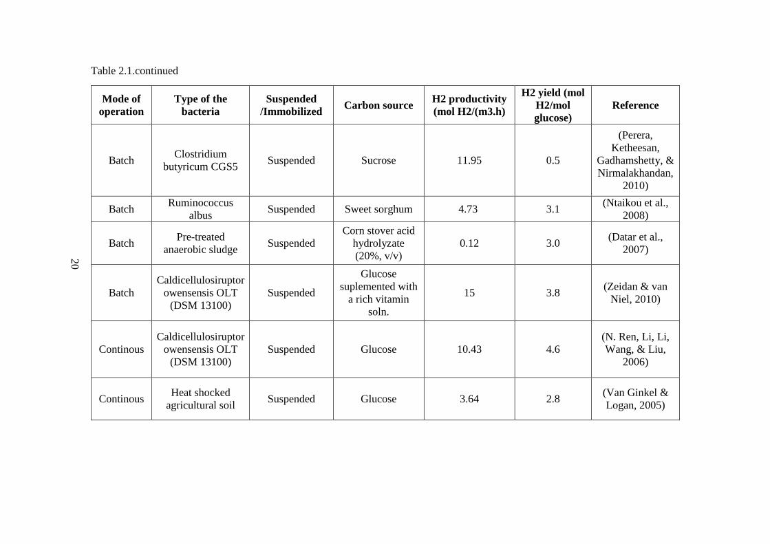
The studies with the highest productivities are highlighted in Figure 2.3. All the studies

shown in Figure 2.3 are given in Table 2.2.

18

Table 2.1: The comparison of dark fermentation studies in terms of their productivities and substrate conversion efficiencies

Mode of

operation

Type of the

bacteria

Suspended

/Immobilized Carbon source

H2 productivity

(mol H2/(m3.h)

H2 yield (mol

H2/mol glucose) Reference

Continuous seed sludge rich in

Clostridium sp. Suspended

Condensed molasses

fermentation solubles 0.02 2.1

(Lay et al.,

2010)

Continuous Sludge Immobilized Molasses from a local

beet sugar refinery 31.91 1.7

(W. Q.

Guo et al.,

2008)

Continuous

Clostridium

butyricum and

Enterobacter

aerogenes

Immobilized Starch (without any

reducing agent) 58.42 2.6

(Yokoi et

al., 1998a)

Batch Enterobacter cloacae

DM11 Immobilized Glucose 29.42 3.3

(Nath et

al., 2008)

Batch

Caldicellulosiruptor

saccharolyticus

DSM 8903

Suspended Molasses 7.1 2.1

(Özgür,

Mars, et

al., 2010)

18

19

Table 2.1.continued

Mode of

operation

Type of the

bacteria

Suspended


H2 productivity

(mol H2/(m3.h)

H2 yield

(mol H2/mol

glucose)

Reference

Batch Clostridium

butyricum KBH1 Suspended

Oil palm empty

fruit branch

molasses

0.92 __ (Abdul et al., 2013)

Batch Pre-heated

activated sludge Suspended

Hydrolyzed

cassava strach 11.79 2.0

(Su, Cheng, Zhou,

Song, & Cen,

2009b)

Batch Anaerobic sludge Suspended Ground wheat

solution 3.11 1.9

(Argun & Kargi,

2010b)

Batch

Anaerobic mixed

bacteria (mainly

Clostridium

species)

Suspended Cassava stach 15.05 2.5

(Cheng, Su, Zhou,

Song, & Cen,

2011)

Batch Clostridium

pasteurianum CH4 Suspended Sucrose __ 1.9

(Chun Yen Chen,

Yeh, Lo, Wang, &

Chang, 2010)

19

20

Table 2.1.continued

Mode of

operation

Type of the

bacteria

Suspended


H2 productivity

(mol H2/(m3.h)

H2 yield (mol

H2/mol

glucose)

Reference

Batch Clostridium

butyricum CGS5 Suspended Sucrose 11.95 0.5

(Perera,

Ketheesan,

Gadhamshetty, &

Nirmalakhandan,

2010)

Batch Ruminococcus

albus Suspended Sweet sorghum 4.73 3.1

(Ntaikou et al.,

2008)

Batch Pre-treated

anaerobic sludge Suspended

Corn stover acid

hydrolyzate

(20%, v/v)

0.12 3.0 (Datar et al.,

2007)

Batch


owensensis OLT

(DSM 13100)

Suspended

Glucose

suplemented with

a rich vitamin

soln.

15 3.8 (Zeidan & van

Niel, 2010)

Continous


owensensis OLT

(DSM 13100)

Suspended Glucose 10.43 4.6

(N. Ren, Li, Li,

Wang, & Liu,

2006)

Continous Heat shocked

agricultural soil Suspended Glucose 3.64 2.8

(Van Ginkel &

Logan, 2005)

20

21

2.3.3 Photofermentation

Purple non sulfur bacteria (PNSB) are able to convert organic acids into H2 and CO2

under anaerobic and nitrogen limited conditions by utilizing sunlight. Some PNSB

commonly used in photofermentation are Rhodopseudomonas palustris (Chun Yen

Chen et al., 2008), Rhodobacter sphaeroides (Redwood & Macaskie, 2006), and

Rhodobacter capsulatus (Androga, Özgür, & Eroglu, 2012; Özgür, Uyar, et al., 2010).

Pure cultures used in photofermentation enables the engineering of the metabolisms

according to the needs (Brentner et al., 2010).

Nitrogenase is the enzyme responsible from hydrogen production in

photofermentation. The following reaction shows the nitrogen fixation by nitrogenase

to produce hydrogen (Androga, Özgür, Eroglu, Gündüz, & Yücel, 2012).

N2 + 8H+ + 8e- + 16 ATP NH3 + H2 + 16 ADP + 16 Pi (2.16)

Under nitrogen limited conditions, nitrogenase works similar to hydrogenase and

catalyzes protons to produce molecular hydrogen. Therefore, under nitrogen limited

conditions, with the same energy consumption, 4 times more hydrogen can be

produced (Androga, Özgür, Eroglu, et al., 2012).

2H+ + 2e- + 4 ATP H2 + 4 ADP + 4 Pi (2.17)

Hydrogen can also be produced via the membrane-bound H2-uptake hydrogenase

through the reversible reaction (Androga, Özgür, Eroglu, et al., 2012):

2H+ + 2e- H2 (2.18)

The metabolic pathway of the hydrogen production is affected by three external

factors: carbon source, light and oxygen availability. PNSB can utilize many carbon

22

sources such as sugars, short chain organic acids, amino acids, alcohol and

polyphenols. The hydrogen production pathway by photofermentation in PNSB is

shown in Figure 2.4. By the oxidation of organic acids, electrons are generated.

Electrons are then transferred to cytochrome c (Cyt c). Then, by passing through a

number of electron transport proteins electrons are transferred to ferredoxin (Fd). At

the same time, protons are pumped through the membranes and a proton gradient is

formed. This gradient triggers the ATP synthase and ATP is produced. Electrons are

transferred to nitrogenase enzyme with the help of ferredoxin and molecular hydrogen

is produced (Androga, Özgür, Eroglu, et al., 2012).

Three different nitrogenase enzymes are known: Nif, Vnf and Anf whose active metals

are Mo, V and Fe, respectively. Besides nitrogenase, hydrogenase is also an important

enzyme in photofermentative hydrogen production, which is responsible for the

oxidation of molecular hydrogen to form protons and the reduction of protons to form

H2. The hydrogenase types are [FeFe]-hydrogenase, [NiFe]-hydrogenase and [Fe]-

hydrogenase. Hydrogen is consumed by [NiFe]-hydrogenase; whereas hydrogen is

produced by the activities of [FeFe]-hydrogenase enzyme (Androga, Özgür, Eroglu, et

al., 2012).

23

Figure 2.4: Hydrogen production pathway by photofermentation in PNSB (Androga,

Özgür, Eroglu, et al., 2012).

PNSB has the ability to utilize sunlight as mentioned above and drive

thermodynamically unfavorable reactions (Brentner et al., 2010). Acetate, which is the

most common carbon source used for photofermentation can be consumed by

photosynthetic bacteria through the following reaction. The theoretical hydrogen yield

is 4 mole of H2 per mole of acetic acid when acetic acid is the only carbon source

(Manish & Banerjee, 2008).

CH3COOH + 2 H2O 4 H2 + 2 CO2 (2.16)

Photosynthetic microorganisms can divert all of the electrons from an organic

substrate. Therefore, high yields are obtained from photofermentation. This is a

noteworthy advantage over dark fermentation (Brentner et al., 2010).

The hydrogen productivities according to years are shown in Figure 2.5. In order to

see the improvement in productivities in years, a comparison of productivities with the

most promising data found from literature is shown in Figure 2.6. In general, hydrogen

productivities in photofermentation are in the order of 1 mol H2/(m3.h).

24

Figure 2.5: Chronological summary of hydrogen productivities in photofermentation

studies

Figure 2.6: Comparison of productivities of photofermentation

25

The major advantages of photofermentation are listed below (Fernandez-Sevilla et al.,

2014):

Oxygen, which inhibits the enzymes responsible for hydrogen production, is

not produced.

A wide variety of organic substrates and waste waters can be utilized.

PNSB can utilize a wide range of the solar spectrum, between 300 to 1000 nm.

Since PNSB are able to utilize all the energy coming from the sunlight to produce

hydrogen, among the biological hydrogen production methods, this mechanism seems

to be the most promising one (Das & Veziroglu, 2001).

Tao et al (2006) reported a productivity of 105 mL H2/L/h (4.72 mol H2/(m3.h). To the

best of our knowledge, this is the highest hydrogen productivity found in literature

among photofermentation studies. In this study, butyrate was the sole carbon source.

Rhodobacter sphaeroides SH2C was used in batch cultures under 4000 lux

illumination, at 30°C and at a pH of 7. The hydrogen yield is found as 6.91 mol H2/mol

butyrate (Tao, et al. 2006)

In another study, hydrogen productivity was found as 1.4 L H2/(L.day) (2.62 mol

H2/(m3.h)) using glucose as the carbon source. The experiment was carried out in batch

cultures for 6 days with Rhodobacter capsulatus JP91 (Ghosh, Sobro, & Hallenbeck,

2012).

Wang et al (2010) used a panel PBR with entrapped gel granules packed within.

Productivity was found as 2.61 mol H2/(m3.h). Immobilized Rhodopseudomonas

palustris CQK 01 on glucose was utilized during the experiment (Wang, Liao, Zhu,

Tian, & Zhang, 2010).

26

Though not directly proportional, the productivity increases as the number of carbon

atoms increases in the substrate, as suggested by Figure 2.4 and Figure 2.5, Therefore,

single stage photofermentation of high carbon substrates could be advantageous.

However, for an economically feasible operation, waste water such as molasses should

be utilized. There are very limited studies in literature about the single stage

photofermentation of molasses. Keskin and Hallenbeck studied the single stage

photofermentation using beet molasses, black strap molasses and sucrose. (Keskin &

Hallenbeck, 2012). Sağır also studied photofermentation by utilizing different

Rhodobacter species (Rhodobacter capsulatus DSM 1710, Rhodobacter capsulatus

YO3 (Hup-), Rhodopseudomonas palustris DSM 127, Rhodobacter sphaeroides

O.U.001 (DSM 5864) ) on 5, 7.5 and 10 mM sucrose containing molasses. The highest

productivity was found as 0.55 mol H2/(m3.h) from Rp. Palustris on 5 mM sucrose

containing molasses, whereas a comparable productivity was found with R. capsulatus

YO3 (0.41 mol H2/(m3.h)) on 5 mM sucrose containing molasses (Sağır, 2012).

The details of the studies shown in Figure 2.5 are given in Table 2.2. Outdoor studies

are also shown in Figure 2.5. The details of outdoor studies are given in Table 5.5.

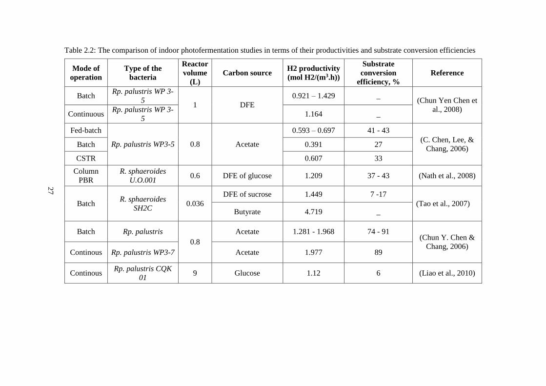
27

Table 2.2: The comparison of indoor photofermentation studies in terms of their productivities and substrate conversion efficiencies

Mode of

operation

Type of the

bacteria

Reactor

volume

(L)

Carbon source H2 productivity

(mol H2/(m3.h))

Substrate

conversion

efficiency, %

Reference

Batch Rp. palustris WP 3-

5 1 DFE

0.921 – 1.429 _ (Chun Yen Chen et

al., 2008) Continuous

Rp. palustris WP 3-

5 1.164 _

Fed-batch

Rp. palustris WP3-5 0.8 Acetate

0.593 – 0.697 41 - 43

(C. Chen, Lee, &

Chang, 2006) Batch 0.391 27

CSTR 0.607 33

Column

PBR

R. sphaeroides

U.O.001 0.6 DFE of glucose 1.209 37 - 43 (Nath et al., 2008)

Batch R. sphaeroides

SH2C 0.036

DFE of sucrose 1.449 7 -17

(Tao et al., 2007) Butyrate 4.719 _

Batch Rp. palustris

0.8

Acetate 1.281 - 1.968 74 - 91 (Chun Y. Chen &

Chang, 2006) Continous Rp. palustris WP3-7 Acetate 1.977 89

Continous Rp. palustris CQK

01 9 Glucose 1.12 6 (Liao et al., 2010)

27

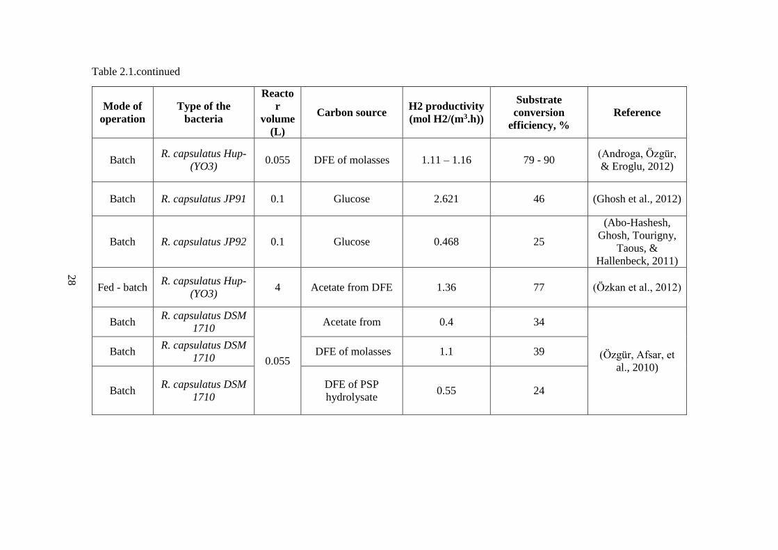
28

Table 2.1.continued

Mode of

operation

Type of the

bacteria

Reacto

r

volume

(L)


(mol H2/(m3.h))

Substrate

conversion

efficiency, %

Reference

Batch R. capsulatus Hup-

(YO3) 0.055 DFE of molasses 1.11 – 1.16 79 - 90

(Androga, Özgür,

& Eroglu, 2012)

Batch R. capsulatus JP91 0.1 Glucose 2.621 46 (Ghosh et al., 2012)

Batch R. capsulatus JP92 0.1 Glucose 0.468 25

(Abo-Hashesh,

Ghosh, Tourigny,

Taous, &

Hallenbeck, 2011)

Fed - batch R. capsulatus Hup-

(YO3) 4 Acetate from DFE 1.36 77 (Özkan et al., 2012)

Batch R. capsulatus DSM

1710

0.055

Acetate from 0.4 34

(Özgür, Afsar, et

al., 2010)


1710 DFE of molasses 1.1 39


1710

DFE of PSP

hydrolysate 0.55 24

28

29

Table 2.1.continued

Mode of

operation

Type of the

bacteria

Reactor

volume

(L)


(mol H2/(m3.h))

Substrate

conversion

efficiency, %

Reference


1710

0.055

DFE of molasses 1.1 39

(Özgür, Mars, et

al., 2010) Batch R. capsulatus hup- DFE of molasses 1.37 58

Batch Rp. palustris

DSM127 DFE of molasses 1.16 46

Batch R. capsulatus hup -

(YO3) 0.055

DFE of barley straw

hyrolysate 0.49 – 0.58 36 - 37

(Özgür & Peksel,

2013)

Batch

R. sphaeroides

O.U.001 (DSM

5864)

0.36 olive mill

wastewater (OMW) 0.288 17

(E. Eroglu,

Gunduz, Yucel, &

Eroglu, 2011)

Batch

R. sphaeroides

O.U.001 (DSM

5864)

1 DL malic acid 0.292 75 (Basak & Das,

2009)

Batch

Rp. palustris WP3-5 0.5

Formate _ _

(Lo, Chen, Lee, &

Chang, 2011)

Acetate 0.571 67

Lactate 0.508 73

Butyrate 0.548 68

Ethanol _ _

29

30

Table 2.1.continued

Mode of

operation

Type of the

bacteria

Reactor

volume

(L)


(mol H2/(m3.h))

Substrate

conversion

efficiency, %

Reference

Batch Rp. palustris CQK

01 0.1

Glucose based

synthetic

wastewater

1.908 6 (Zhang et al., 2010)

Batch Rp. palustris CQK

01 0.8 Glucose 2.61 30

(Y. Z. Wang et al.,

2010)

Continuous Rp. palustris CQK

01 0.125 Glucose 0.74 - 1.75 _

(C. L. Guo et al.,

2011)

Batch Rp. palustris 0.25 DFE 0.737 7 (Su et al., 2009b)

Batch R. Spheroides RV 0.31 DFE 0.392 22 (Argun & Kargi,

2010b)

Batch R. sphaeroides 0.055 DFE 1.317 40 (Afsar et al., 2011)

Batch R. palustris WP3-5 DFE 0.567 18 (Perera et al., 2010)

Continous R. palustris WP3-6 DFE 0.292 21

Repeated

batch

R. sphaeroides M-

19 0.05 DFE __ 37 -38 (Yokoi et al., 2001)

30

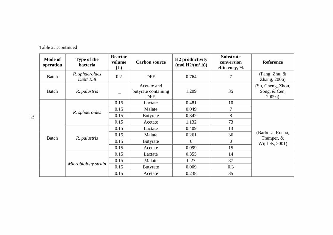
31

Table 2.1.continued

Mode of

operation

Type of the

bacteria

Reactor

volume

(L)


(mol H2/(m3.h))

Substrate

conversion

efficiency, %

Reference

Batch R. sphaeroides

DSM 158 0.2 DFE 0.764 7

(Fang, Zhu, &

Zhang, 2006)

Batch R. palustris _

Acetate and

butyrate containing

DFE

1.209 35

(Su, Cheng, Zhou,

Song, & Cen,

2009a)

Batch

R. sphaeroides

0.15 Lactate 0.481 10

(Barbosa, Rocha,

Tramper, &

Wijffels, 2001)

0.15 Malate 0.049 7

0.15 Butyrate 0.342 8

0.15 Acetate 1.132 73

R. palustris

0.15 Lactate 0.409 13

0.15 Malate 0.261 36

0.15 Butyrate 0 0

0.15 Acetate 0.099 15

Microbiology strain

0.15 Lactate 0.355 14

0.15 Malate 0.27 37

0.15 Butyrate 0.009 0.3

0.15 Acetate 0.238 35

31

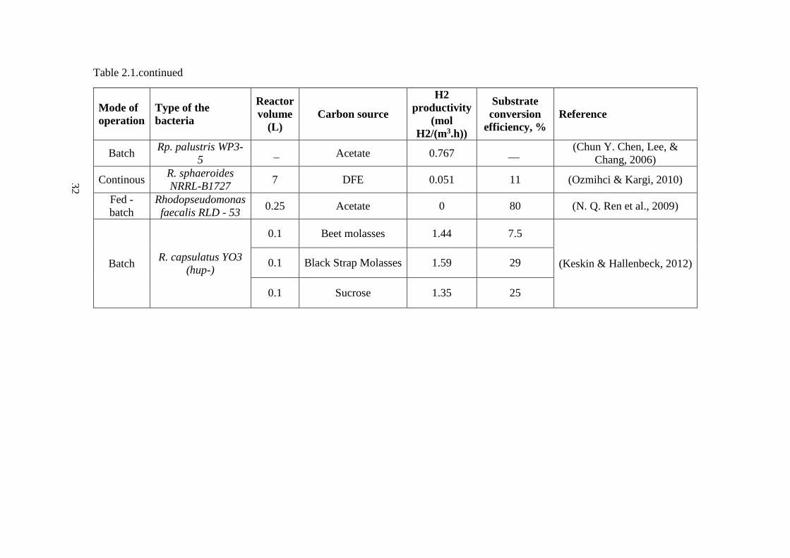
32

Table 2.1.continued

Mode of

operation

Type of the

bacteria

Reactor

volume

(L)

Carbon source

H2

productivity

(mol

H2/(m3.h))

Substrate

conversion

efficiency, %

Reference

Batch Rp. palustris WP3-

5 _ Acetate 0.767 __

(Chun Y. Chen, Lee, &

Chang, 2006)

Continous R. sphaeroides

NRRL-B1727 7 DFE 0.051 11 (Ozmihci & Kargi, 2010)

Fed -

batch

Rhodopseudomonas

faecalis RLD - 53 0.25 Acetate 0 80 (N. Q. Ren et al., 2009)

Batch R. capsulatus YO3

(hup-)

0.1 Beet molasses 1.44 7.5

(Keskin & Hallenbeck, 2012) 0.1 Black Strap Molasses 1.59 29

0.1 Sucrose 1.35 25

32

33

2.3.4 Integrated Systems

The organic acids produced in dark fermentation could be utilized in

photofermentation to increase hydrogen yield. Since this is a two stage process, it is

not practical to report productivity for sequential dark and photofermentation. 12

moles of hydrogen can be produced from one mole of glucose by sequential dark and

photofermentation as shown in the following equation (Argun & Kargi, 2011; Manish

& Banerjee, 2008).

CH3COOH + 2 H2O 4 H2 + 2 CO2 (2.16)

When only acetic acid is produced, 24 mole of hydrogen could be produced from one

mole of sucrose. The overall reaction is obtained by summing up the Reactions 2.15

and 2.16 (Urbaniec & Grabarczyk, 2014).

C12H22O11 + 13 H2O 24 H2 + 12 CO2 (2.17)

Urbaniec and Grabarczyk (2013) studied the economics of a hydrogen production

plant utilizing dark fermentation followed by photofermentation. The economic

analysis was done for a hypothetical plant with 60 kg/h H2 production capacity which

corresponds to 2000 kW. In this hypothetical plant, hydrogen was produced at a rate

of 10 h/day. As it can be seen from Figure 2.7, hydrogen production cost was mainly

due to capital cost. This capital cost included land price and equipment cost. The large

land area occupied by the PBR was the main reason of this high capital cost. 93 % of

the capital cost was due to photofermentation Figure 2.8). Urbaniec and Grabarczyk

(2013) investigated a manifold type tubular PBR with LDPE channels that is used in

the work of Boran (Boran, Özgür, Yücel, Gündüz, & Eroglu, 2012a, 2012b) They

found that LDPE tubes are the main operating cost item as shown in Figure 2.9.

Therefore, in the light of this work, it could be concluded that the reactor used in

photofermentation needs to be improved for an economically feasible operation

(Urbaniec & Grabarczyk, 2014).

34

Figure 2.7: Cost items for two-stage biological H2 production

Figure 2.8: Breakdown of capital costs for two-stage biological H2 production

Figure 2.9: Operating costs for photofermentation

7,04

52,11

36,4

4,45

0

10

20

30

40

50

60

Raw material Capital Operating Labor

Contr

ibuti

on (

%)

5,6

92,68

1,720

20

40

60

80

100

Thermophilic

fermentation

Photofermentation Gas upgrading

Contr

ibuti

on (

%)

14,32

64,65

3,6

11,624,84

0,970

10

20

30

40

50

60

70

Contr

ibuti

on

(%

)

35

2.3.5 Mixed Cultures for Simultaneous Dark and Photofermentation

Instead of using two different reactors for dark and photofermentation, researchers

have also tried to use co-cultures of dark and photo fermentation bacteria. Asada et al

(2006) co-immobilized Lactobacillus delbrueckii NBRC13953 and Rhodobacter

sphaeroides-RV and found a productivity of 1.89 mol H2/m3/h. Glucose was used as

the carbon source. The maximum yield was reported as 7.1 mol H2/mol glucose [73].

Ding et al (2009) reported a maximum productivity of 33.85 ml H2/(L.h) (1.52 mol

H2(m3.h) obtained by using 6 g/L glucose. Co – culture of Clostridium butyricum and

immobilized Rhodopseudomonas faecalis RLD – 53 was utilized under 8000 lux

illumination. The ratio of dark to photo bacteria was 1:10. The hydrogen yield was

reported as 4.13 mol H2/mol glucose (Ding et al., 2009).

Productivity reported in literature for combined dark and photofermentation is up to 2

mol H2/m3/h (Figure 2.10).

36

Figure 2.10: Chronological summary of hydrogen productivities in mixed cultures for

simultaneous dark and photofermentation

The studies with the highest productivity are highlighted in Figure 2.10. The details of

all the studies depicted in Figure 2.10 are given in Table 2.3.

37

Table 2.3: Comparison of productivities and yields for mixed cultures for simultaneous dark and photofermentation

Mode of

operation Type of the bacteria

Suspended

/Immobilized

H2 productivity

(mol H2/(m3.h) Feed

H2 yield (mol

H2/mol

glucose)

Reference

Batch

Clostridium butyricum DSM

10702 and Rhodobacter

sphaeroides DSM 158 Suspended 0.34

Glucose (5

g/ L) 0.86

(Fang et al.,

2006)

Batch

Clostridium butyricum

andRhodopseudomonas faecalis

RLD-53 Suspended 0.936

Glucose (9

g/ L) 1.98

(Liu et al.,

2010)

Batch

Clostridium acidisoli and

Rhodobacter sphaeroides Suspended 3.12

Sucrose

(11.43 g /

L) 5.08

(Sun et al.,

2010)

Batch

Anaerobic sludge and

Rhodobacter sp. RV Suspended 0.301

Ground

wheat

starch (4.3

g/ L) 1.45

(Argun &

Kargi, 2010a)

Batch

Anaerobic sludge and mixture

of Rhodobacter sp (NRRL B-

1727) Rhodobacter sp (DSMZ-

158) Rhodopseudomonas

palustris (DSMZ-127)


Ground

wheat

starch (4.1

g /L) 1.16

(Argun, Kargi,

& Kapdan,

2009)

37

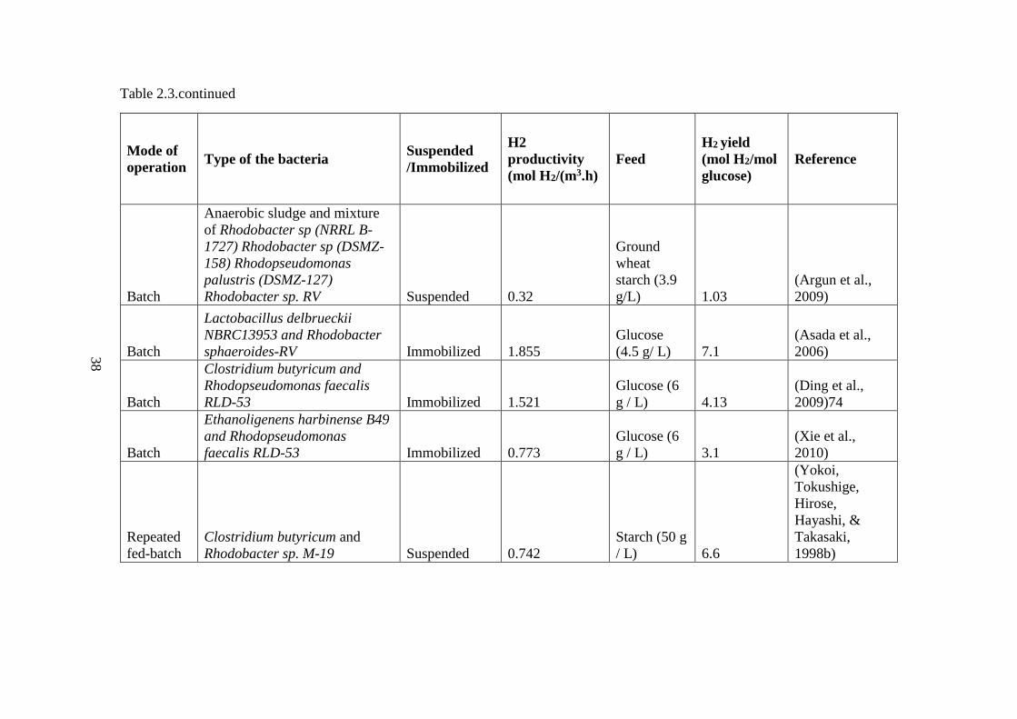
38

Table 2.3.continued

Mode of

operation Type of the bacteria

Suspended

/Immobilized

H2

productivity

(mol H2/(m3.h)

Feed

H2 yield

(mol H2/mol

glucose)

Reference

Batch

Anaerobic sludge and mixture

of Rhodobacter sp (NRRL B-

1727) Rhodobacter sp (DSMZ-

158) Rhodopseudomonas

palustris (DSMZ-127)


Ground

wheat

starch (3.9

g/L) 1.03

(Argun et al.,

2009)

Batch

Lactobacillus delbrueckii

NBRC13953 and Rhodobacter

sphaeroides-RV Immobilized 1.855

Glucose

(4.5 g/ L) 7.1

(Asada et al.,

2006)

Batch

Clostridium butyricum and

Rhodopseudomonas faecalis

RLD-53 Immobilized 1.521

Glucose (6

g / L) 4.13

(Ding et al.,

2009)74

Batch

Ethanoligenens harbinense B49

and Rhodopseudomonas

faecalis RLD-53 Immobilized 0.773

Glucose (6

g / L) 3.1

(Xie et al.,

2010)

Repeated

fed-batch

Clostridium butyricum and

Rhodobacter sp. M-19 Suspended 0.742

Starch (50 g

/ L) 6.6

(Yokoi,

Tokushige,

Hirose,

Hayashi, &

Takasaki,

1998b)

38

39

2.4 Photobioreactors for Hydrogen Production

Photobioreactors (PBRs) are reactors in which photosynthetic microorganisms are

cultivated, utilizing a light source. PBRs can be open systems such as raceway ponds,

lagoons and lakes, or closed systems such as flat plate and tubular. Since anaerobic

conditions are necessary, open systems are not suitable for photofermentative

hydrogen production. The key parameters in the design of PBRs can be listed as

follows (Androga, Özgür, Eroglu, et al., 2012).

The reactor material should be impermeable to hydrogen and air.

The reactor material should transmit light easily.

The reactor material should be inert and durable under outdoor conditions.

The surface to volume ratio should be as high as possible.

Panel and tubular PBRs are the two commonly used reactor types for

photofermentative hydrogen production (Androga, Özgür, Eroglu, et al., 2012).

2.4.1 Panel Photobioreactors

Panel PBRs consists of two transparent plates (e.g. PMMA or glass) that are attached

to each other by a frame (Androga, Özgür, Eroglu, et al., 2012). Illuminated surfaces

are typically oriented in the east – west direction for the efficient use of sunlight, since

purple non sulfur bacteria mainly utilize long wave radiation which is more dominant

in the morning and in the evening. The spacing between the panels is adjusted

according to the targeted light and temperature distribution. The hydrostatic pressure

at the bottom limits the panel height (I. Eroglu et al., 2014). A typical panel PBR is

shown in Figure 2.11.

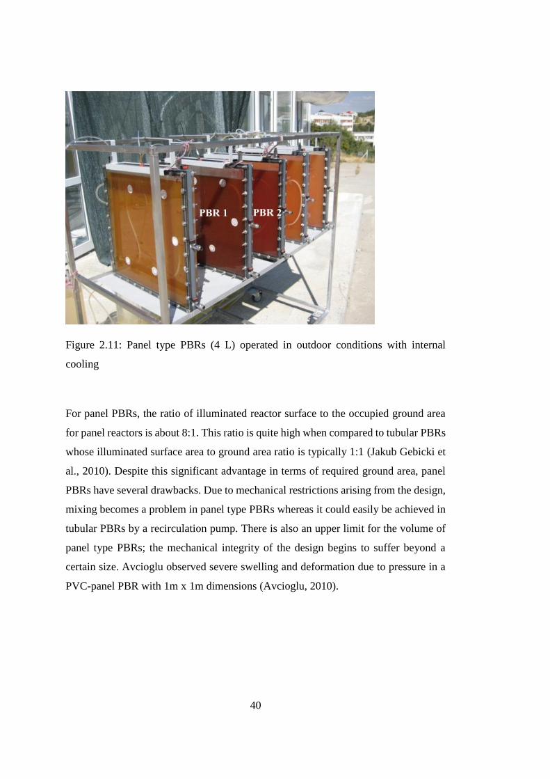
40

Figure 2.11: Panel type PBRs (4 L) operated in outdoor conditions with internal

cooling

For panel PBRs, the ratio of illuminated reactor surface to the occupied ground area

for panel reactors is about 8:1. This ratio is quite high when compared to tubular PBRs

whose illuminated surface area to ground area ratio is typically 1:1 (Jakub Gebicki et

al., 2010). Despite this significant advantage in terms of required ground area, panel

PBRs have several drawbacks. Due to mechanical restrictions arising from the design,

mixing becomes a problem in panel type PBRs whereas it could easily be achieved in

tubular PBRs by a recirculation pump. There is also an upper limit for the volume of

panel type PBRs; the mechanical integrity of the design begins to suffer beyond a

certain size. Avcioglu observed severe swelling and deformation due to pressure in a

PVC-panel PBR with 1m x 1m dimensions (Avcioglu, 2010).

41

2.4.2 Tubular Photobioreactors

Tubular PBRs have long transparent tubes whose diameters are in the range of 3 to 6

cm with the length of the tubes ranging from 10 to 100 m (Akkerman, Janssen, Rocha,

& H, 2002). Different types of tubular PBRs are shown in

Figure 2.12. Tubular PBRs could be vertical, horizontal, nearly horizontal, helical or

α-shaped. Bubble column and airlift reactors are examples of vertical PBRs. In vertical

type PBRs, a gas is generally supplied to the system for mixing purposes. However,

these systems are not suited well to photofermentative hydrogen production, since any

inert gas supplied to the system will dilute the product gas and require additional costs

for separation. Horizontal tubular PBRs are preferred since they can utilize sunlight

with high light conversion efficiency. Helical PBRs are made up of flexible materials.

Cooling is achieved by an external heat exchanger. In α-shaped helical reactors, the

liquid is raised to a reservoir and flows down using an inclined tube. The liquid is

collected in another air riser. Then the process is repeated (Dasgupta et al., 2010).

Some tubular PBRs are nearly horizontal, and have several parallel tubes connected to

each other by manifolds. Mixing is achieved by recirculation of the liquid culture

medium. An example of such a tubular PBR operated in outdoors on thick juice dark

fermenter effluent is shown in Figure 2.13 (Boran et al., 2012b). Androga modelled

flow in this manifold type PBR for a 255 mL/min volumetric recirculation rate. The

results (Figure 2.14 and Figure 2.15) showed that the flow distribution among the tubes

differs considerably. (Androga, 2014).

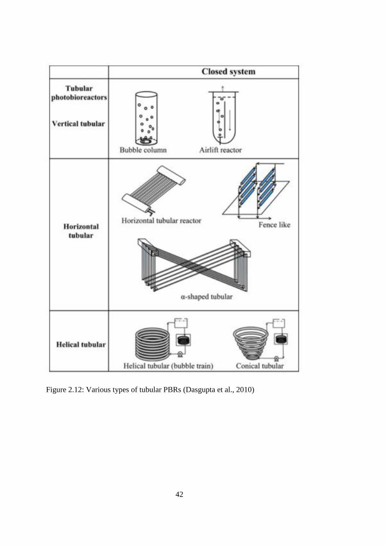
42

Figure 2.12: Various types of tubular PBRs (Dasgupta et al., 2010)

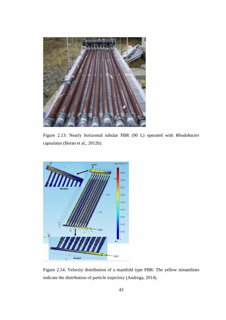
43

Figure 2.13: Nearly horizontal tubular PBR (90 L) operated with Rhodobacter

capsulatus (Boran et al., 2012b).

Figure 2.14: Velocity distribution of a manifold type PBR. The yellow streamlines

indicate the distribution of particle trajectory (Androga, 2014).

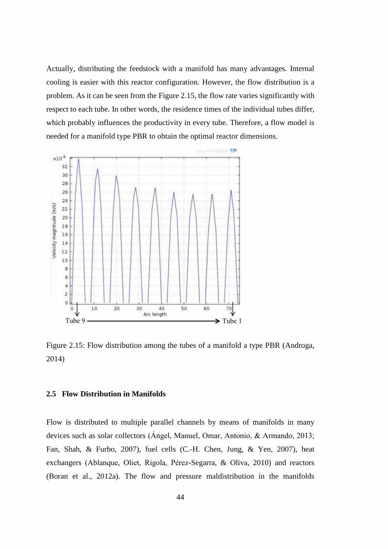
44

Actually, distributing the feedstock with a manifold has many advantages. Internal

cooling is easier with this reactor configuration. However, the flow distribution is a

problem. As it can be seen from the Figure 2.15, the flow rate varies significantly with

respect to each tube. In other words, the residence times of the individual tubes differ,

which probably influences the productivity in every tube. Therefore, a flow model is

needed for a manifold type PBR to obtain the optimal reactor dimensions.

Figure 2.15: Flow distribution among the tubes of a manifold a type PBR (Androga,

2014)

2.5 Flow Distribution in Manifolds

Flow is distributed to multiple parallel channels by means of manifolds in many

devices such as solar collectors (Ángel, Manuel, Omar, Antonio, & Armando, 2013;

Fan, Shah, & Furbo, 2007), fuel cells (C.-H. Chen, Jung, & Yen, 2007), heat

exchangers (Ablanque, Oliet, Rigola, Pérez-Segarra, & Oliva, 2010) and reactors

(Boran et al., 2012a). The flow and pressure maldistribution in the manifolds

45

significantly affect the performance of such systems. With an optimal manifold design,

an increase in efficiency and a reduction in the operation cost could be accomplished.

The geometric configuration of the manifold affects the flow distribution. Manifolds

can be divided into two general groups in terms of their configuration: U-type (reverse)

(J. Wang, 2008) and Z-types (parallel) (J. Wang, 2010) as shown in Error! Reference

ource not found.. Manifolds could be placed vertically or horizontally.

Figure 2.16: (a) U type manifolds (b) Z type manifolds

The flow distribution in the manifold for a single phase flow is determined by the wall

friction and momentum changes. In the distribution manifold, as the fluid moves along

the manifold, friction increases, whereas the fluid loses momentum with the loss of

fluid to the channels. In the collection manifold, both the momentum and friction

effects work in the same direction, as the fluid moves towards the outlet. The pressure

also changes along the manifold due to friction and momentum effects. Pressure

decreases in the direction of the fluid due to friction whereas momentum effects tend

to rise the pressure along the distribution manifold. In the collection manifold, both

friction and momentum effects cause pressure drop towards the outlet (Acrivos,

Babcock, & Pigford, 1959). In the manifold design, the dimensions of the distribution

manifold are the main design criterion, since it is important to balance the momentum

and friction effects. However, it is important to understand the combined frictional and

momentum effects in the collection manifold. The findings of Ahn et al (1997) also

(a) (b)

46

confirms that the diameter to length ratio of the distribution manifold affects the flow

distribution more than the dimensions of combination manifold does (Ahn et al.,

1998). Acrivos and his coworkers observed a pressure rise near the channel outlet in

the collection manifold experimentally (Acrivos et al., 1959).

The pressure and flow characteristics in a manifold can be modeled by means of

discrete models (network models), analytical models and computational fluid

dynamics (CFD). In discrete models, the manifold consists of multiple junctions.

Momentum, mass and energy conservation equations are solved at each junction

(Ablanque et al., 2010). Analytical models, also called continuous models, represent

the domain in a continuous manner. In analytical models, the mass, momentum and

energy conservation equations are written for a control volume, and differential

equations are obtained from these equations. Analytical models are the fundamentals

of most of the discrete models. As the number of junctions approaches infinity in

discrete models, analytical models are obtained (J. Wang, 2011). In CFD, the geometry

is discretized and conservation of mass, momentum and energy equations are solved

at each mesh point. Then, a global solution is obtained by combining the information

of each mesh point (Ahn et al., 1998; Comsol, 2012b; Fan et al., 2007) In the following

paragraphs, different manifold models found in literature are mentioned. The effects

of different parameters on the flow distribution are given.

Acrivos, Babcock, and Pigford (1959) modelled the flow distribution in a manifold

using both a discrete and an analytical model. 3 parameters were investigated in this

study: momentum flow (ratio of fluid pressure to specific kinetic energy) at the

entrance (M0), the friction in the straight tube section (F0) and the spacing between the

channels (s). (For notational consistency, Δy in the work of Acrivos et al. is changed

with s). M0 could be changed by changing the entrance velocity. From the results of

Acrivos and his coworkers, it was found that there was no pair of F0 and M0 that would

make a perfect uniform distribution. Therefore, the aim should be obtaining the most

uniform flow distribution as possible. Acrivos et al (1959) changed the spacing

47

between the channels by decreasing the channel number. They found that increasing

the spacing provides a more uniform distribution until the distance became so great

that the friction effects becomes significant (Acrivos et al., 1959).

Ablanque et al (2010) studied the flow distribution in manifolds using a discrete model.

The domain discretization is shown in Figure 2.17. Two types of discretization were

used: higher level and lower level discretization. In higher level discretization, T-

junction models were solved, whereas in lower level discretization, the tube is

branched and 2-phase flow models are solved. With the global model, three different

numerical models were coupled. First, at the T-junctions, the pressure change

(distribution and collection manifolds) and phase split (in two-phase flow distribution

junctions) were predicted. Secondly, the continuity, momentum conservation and

energy conservation equations were solved through the tubes. Finally, the equations

solved for the tubes and the junctions were coupled with the global momentum

conservation and continuity equations (Ablanque et al., 2010).

Figure 2.17:Domain discretization (a) higher level discretization in T-junctions (b)

lower level discretization in the tubes (Ablanque et al., 2010)

Ablanque et al. (2010) studied single phase flow for two different tube pitches (0.1 m

and 1 m) for reverse (U type) and parallel (Z type) manifold configurations and

compared their results with the model developed by Wang and Yu (1989). Wang and

Yu (1989) also performed some experiments to validate the model. The working fluid

48

was water. Both the manifold and the tubes were held horizontal. 10 parallel tubes with

12.5 mm diameter and 3 m length were used. The distribution manifold diameter was

25 mm. The inlet flow rate was 0.227 kg/s. The error between the experimental data

of Wang and Yu (1989) and the corresponding predictions made by Ablanque et al.

(2010) were lower than 8%. Ablanque et al. compared their model results with the

model results of Wang and Yu. The most uniform flow distribution is obtained with

reverse configuration (U-type) and smaller pitch (E=0.1). It is concluded from the

results that the flow distribution is remarkably affected by the distribution manifold

pressure profile (Ablanque et al., 2010; X. A. Wang & Yu, 1989).

Ablanque et al. also modelled the two phase flow and compared the model results with

the experiments performed by Sivert (2003). The working fluid was water and carbon

dioxide. Horizontal manifold with vertical tubes was used. The manifold configuration

was reverse. 10 parallel tubes with 4 mm in diameter and 0.9 m in length were utilized.

The distribution manifold diameter was 16 mm. The inlet mass flow rate was 0.033

kg/s. Different inlet gas fractions such as 0.14, 0.28, 0.43 and 0.54 were used. The

mean prediction error in two phase flow was 32 %. Although this value was

significantly high, Ablanque et al. managed to predict the general trends (Ablanque et

al., 2010; Sievert, 2003).

Wang (2011) studied the flow distribution in a manifold using an analytical model.

Wang tried to obtain the most generalized equations defining the flow inside the

distribution and collection manifolds by reviewing the literature in the past fifty years.

Wang (2011) developed a model by unifying the models developed by Acrivos (1959),

Wang (2008) and Wang (2010). Wang (2011) claimed that they developed the most

generalized equations for distribution and collection manifolds (Equations 19 and 20

in Wang (2011)). Varying friction and pressure recovery factors can be adopted to

their model. Wang (2011) studied effect of 3 characteristic parameters (E, M and ζ)

and Reynolds number on flow distribution and pressure drop. E is defined as the ratio

of the manifold length to diameter. M is the ratio of all the port areas to the area of the

49

manifold. ζ is average total head loss coefficient for port flow. Their results show that

momentum and friction effects work in opposite directions and these parameters needs

to be adjusted in order to obtain a uniform flow distribution. 3 different E values (3, 5

and 100) were studied when Re, M and ζ were 2000, 2 and 2 respectively. Wang (2011)

found that as E increases the friction term becomes dominant and the flow distribution

tends to distribute unequally. By studying 3 different M values (0.5, 2 and 3), Wang

(2011) concluded that as M was increased, the flow was distributed to the ports

unequally. As M increases, the momentum effects became significant and they could

not balance the friction effects. In order to obtain a uniform a flow distribution, ζ needs

to be high also. As ζ approaches infinity, the most uniform flow distribution is

expected in the distribution manifold, since there will be no flow branching. Wang

(2011) also studied the effect of Reynolds number. He found that the effect of

Reynolds number increases as M decreases. An increase in Reynolds number causes a

decrease in the friction term and an increase in the pressure recovery factor (J. Wang,

2011). Therefore, it can be concluded that momentum and friction affects the flow

distribution in the manifold. Their effects are in opposite direction. As the length of

the manifold increases, the effect of the friction becomes significant in the distribution

manifold. The fluid loses momentum as it branches to the pipes. When the length of

the distribution manifold is smaller, the flow distribution is mainly affected by the

momentum.

Ahn et al (1997) studied the flow distribution in manifolds for low Reynolds numbers

by using a CFD approach. They modelled a manifold which has 8 parallel pipes by

utilizing Fluent 4.3. Water was the working fluid. They studied the effect of 2

structural parameters ac and ad which were defined as the ratio of the diameter to length

in the distribution and collection manifolds, respectively. Ahn and his coworkers

(1997) found a correlation for uniform flow distribution. They studied 3 different

values of ac and ad which are 1/16, 1/8 and 1/4 while keeping Reynolds number in the

pipes as constant at 100. As ad decreases the flow tends to go through the channels that

are closest to the entrance. Ahn and his coworkers found that the effect of the pipe

length in the flow distribution was insignificant since the resistance caused by the

50

length of the pipes was smaller than the resistance of the manifolds. ad was found as

the main parameter affecting the flow distribution in this model. Ahn et al (1998) also

conducted an experiment and compared their model results with the experimental

results. The measured flow rates in the parallel pipes showed a great agreement with

the model (Ahn et al., 1998).

Fan, Shah and Furbo (2007) investigated the flow and temperature distribution in a

solar collector panel by using CFD, and compare their model results with their

experimental results. They used different operating parameters such as flow rate,

properties of solar collector fluid (water to glycol ratio), inlet fluid temperature and

collector tilt angle. The distribution manifold and collection manifold diameter were

both 0.0256 m. 16 quadrangular absorber tubes with a hydraulic diameter of 0.0067 m

were used. U tube configuration was used. They used Equation 2.1 while calculating

the flow maldistribution. The definition of flow non-uniformity parameter, Φ, was

similar to the standard deviation with the only difference that non-uniformity

parameter is divided by the mean value (1/N) (Fan et al., 2007).

Φ = √∑ (βİ−1/N)2N

İ=1

N x N x 100 % (2.1)

In a previous study, the flow non-uniformity parameter ( ), shown in Equation 2.1

was defined to quantify the flow distribution. This parameter is analogous to standard

deviation and could be defined as the fractional volumetric flow rate when the flow is

distributed equally to all channels (Fan et al., 2007).

In Equation 2.1, N is the number of channels and β is the dimensionless volumetric

flow rate defined by Equation 2.2.

βi =Qi

Q0 (2.2)

where Q0 is the total volumetric flow rate, and Qi is the flow rate of the ith channel.

51

In order to understand the effect of the buoyancy forces better, Fan and his coworkers

introduced the ratio of Grashof number (Gr) to square root of Reynolds number (Re2).

When this ratio is larger than unity, it could be concluded that buoyancy forces affects

the flow distribution (Fan et al., 2007).

Fan and his coworkers studied 5 different inlet flow rates: 2.5, 4.0, 10.0 and 25.0 L/min

with constant temperature of 60ºC. They observed that the relative flow non-

uniformity parameter increases from 2.8 % to 6.4 % when the flow rate increases from

2.5 L/min to 25.0 L/min. In order to investigate the effects of collector tilt angle, 40º

inclination was given to the collector panel. The collector panel was heated with a solar

radiation of 800 W/m2 and the ambient temperature was 20ºC. It was concluded that

for lower flow rates, the effect of buoyancy forces are high. The most uniform flow

distribution was observed when the inlet flow rates were 10.0 L/min and 25.0 L/min.

53

CHAPTER 3

STACKED U-TUBE PHOTOBIOREACTOR DESIGN

3.1 Design Strategy

3.1.1 Reactor Selection

In order to gain acceptance as a viable route for hydrogen production,

photofermentative hydrogen production has to be implemented in large-scale PBRs

under natural sunlight. Up to now, many of the problems encountered in large scale

outdoor operations have been identified (Adessi, Torzillo, Baccetti, & De Philippis,

2012; Avcıoglu, Özgur, Eroglu, Yücel, & Gündüz, 2011; Boran et al., 2012a).

Running PBRs in outdoor conditions introduces complications such as fluctuating

temperature and light intensity values, which limits productivity. Moreover, large scale

applications differ from the small scale ones in terms of light distribution, reactor

material, gas collection and mixing.

In this part the thesis, issues related to the scale up of PBRs are reviewed and

accordingly, a new reactor design is proposed. Some of these issues are discussed

below.

The effect of temperature on photofermentative hydrogen production has previously

been investigated via small-scale experiments under fluctuating temperatures in the

54

range of 15ºC and 40ºC, using wild type Rhodobacter capsulatus and its hup- mutant.

Furthermore, the bacteria were subjected to 16 h light and 8 h dark cycles in order to

mimic the diurnal cycle. As control, bacteria were grown under continuous

illumination and a constant temperature of 30ºC. The variation in temperature

decreased the hydrogen productivity from 0.7 mol H2 /(m3.h) to 0.25 mol H2/(m

3.h).

The light/dark cycles further decreased the productivity to 0.2 mol H2/(m3.h). The

authors hypothesized that the bacteria spent some of its energy for adaptation to the

temperature changes and light/dark cycles (Özgür, Uyar, et al., 2010).

Light/dark cycles are inevitable in outdoor operation, but their effects are relatively

minor compared to the impact of temperature extremes, especially during summer

months, which are usually preferred for outdoor campaigns due to the abundance of

sunlight. With efficient cooling systems, however, the decrease in productivity due to

temperature fluctuations could be mitigated. A study has been implemented where the

reactor temperature was kept under 30, 33, 35 and 40 oC by shading or water spraying.

The highest productivity (0.32 mol H2/(m3.h)) was obtained when the reactor

temperature was kept at 33ºC or lower; on the other hand, the lowest productivity was

observed to be 0.22 mol H2/(m3.h), when the reactor temperature was allowed to reach

as high as 40ºC (Özgür, Uyar, et al., 2010).

Light distribution within the PBR is critical for scale-up. For large culture depths, light

penetration to the inner regions of the PBR becomes the limiting factor for

productivity. Furthermore, when the available light is below a certain threshold, the

bacteria could shift to completely unfavorable metabolic modes such as dark-

fermentation. This could be prevented by increasing the surface to volume (or length

to thickness) aspect ratio of the PBRs (Androga, Özgür, Eroglu, et al., 2012). In one

study, hydrogen production rates were measured using Roux bottles of varying depths.

Hydrogen production was observed mainly at bottles with depths smaller than 1.5 cm

(Nakada, Asada, Arai, & Miyake, 1995). It should be kept in mind, however, that high

surface-to-volume ratios will increase the required land area, and may complicate the

55

reactor construction and operation. Therefore a total thickness of 3 cm would be a

proper compromise between good light distribution and limited surface area.

Another factor to consider is gas and more specifically hydrogen, permeability.

Especially in large-scale systems, hydrogen loss through the reactor walls should be

reduced as much as possible due to safety and economic considerations. Since a large

surface area is inevitable due to light penetration requirements, it is necessary to

decrease the permeability of the material as much as possible. The hydrogen

permeability of the candidate PBR materials was assessed and experimentally verified

in a previous study (Avcioglu, 2010). The permeability of poly (methyl methacrylate)

(PMMA), glass, polyurethane (PU), polyvinyl chloride-plasticized (PVC-plasticized)

and low-density polyethylene (LDPE) are 1.88x10-14, 4.38x10-16, 2.78x10-12, 4.86x10-

11 and 2.30x10-11 mol/(m.s.Pa). Among these materials, glass was found as the least

permeable material and LDPE the most permeable, thus indicating glass is the best

choice for the reactor material based on permeability. Apart from permeability, glass

is also more advantageous in terms of mechanical strength and durability; it has been

reported that the LDPE reactor tubes used in a previous study (Boran et al., 2010,

2012a) had to be changed every year and the contribution of these tubes to the

operating cost was around 65% (Urbaniec & Grabarczyk, 2014).

As the reactor volume increases, product-gas collection also becomes a problem. It has

been observed that as the reactor headspace pressure increased, hydrogen productivity

decreased (Li et al., 2011). Therefore, it is important to maintain the total gas pressure

in the headspace as low as possible, which will also promote lower retention of the

produced gas, thereby decreasing the loss of hydrogen through the walls due to

permeation as discussed above.

Mixing is promoted in PBRs in order to increase the mass transfer rate, to reduce

nutrient gradients, to eliminate cell sedimentation and to facilitate the separation of the

56

produced gas from the liquid culture. On the other hand, there appears to be an

optimum mixing power value, above which productivity starts to decline. Though the

reasons for the decrease of productivity at elevated mixing power values are unclear,

one possibility is that shear stress, which depends on Reynolds number, induces cell

damage. In a study aimed to probe the effects of mixing, the performances of reactors

shaken at 40, 80, 120 and 160 rpm were monitored and the average productivity was

found to be the highest 2.7 mol H2/(m3.h) when the shaking velocity was 120 rpm

(Flickinger, 2013). This value was significantly higher than that of the control

experiment with no shaking, reported as 1.86 mol H2/(m3.h) (Li et al., 2011). In

tubular PBRs, it has also been reported that hydrogen production is affected by the

volumetric flow rate of recirculation that is used to promote mixing (Jakub Gebicki et

al., 2010). When the Reynolds number was varied from 10 to 6000, the highest

productivity was observed for a Reynolds number of 240. No hydrogen production

was observed when the volumetric flow rate was larger than 2400. However, these

experiments were carried out with a manifold type of PBR where flow distribution

among the channels changed significantly with the Reynolds number. Consequently,

the optimum Reynolds number for other systems should be obtained individually for

other geometries. A flow model is especially useful in this regard, to obtain more

insight into how the velocity distribution depends on the geometry.

Finally, economics is still the main obstacle, preventing the application of such

photofermentative hydrogen production systems in industrial scale. The large ground

area required for a manifold type tubular PBR by photofermentation was the reason of

capital cost of photofermentation being several times larger than dark fermentation.

Therefore, the ground area for the PBR should be reduced (Urbaniec & Grabarczyk,

2014).

Based on the factors discussed up to this point, it can be argued that tubular reactors

offer superior characteristics with respect ease of mixing. Thus, in this work, a pilot-

scale manifold type glass stacked U-tube PBR was designed, built and operated. An

57

upright orientation was selected to ensure small ground area to volume ratio with a

large illuminated surface area, and the reactor material was chosen as glass for

durability and low permeability to hydrogen and air. In designing the tubular PBR

geometry, a hydrodynamic model was used to assess whether a low overall pressure

drop and a uniform velocity distribution could be achieved throughout the reactor and

the dimensions of the reactor was based on the results of the model. The PBR was then

constructed and run with and without bacteria, the latter grown using a molasses

solution as a complex substrate.

3.1.2 Method of Attack

While designing the PBR, the following procedure was followed.

The reactor geometry was selected. Tubular reactors were found more

advantageous, since it is easy to mix the reactor contents. Tubular reactors are

also easier to scale up when compared with the panel type reactors. As

discussed in the literature survey part, tubular PBRs also seem to be more

advantageous in terms of durability and ease of cooling.

Manifolds are preferred to distribute the flow.

The design parameters were selected for a manifold type reactor. Diameter to

length ratio of the manifolds, tube pitch, tube length and the volumetric flow

rate were the parameters that are widely studied in literature for designing

manifolds.

A flow model was solved for the manifold type tubular reactor (stacked U-

tube PBR) via COMSOL Multiphysics 4.4.

The velocity and pressure profile of the reactor was determined from the

model.

The dimensions of the reactor were determined from the model which gave

the most uniform flow distribution among the tubes.

58

The reactor materials used for PBRs were investigated. The ideal reactor

material should have low hydrogen and air permeability. It should have low

cost, and it should be durable in outdoor conditions. The most appropriate

material meeting these needs was found as glass.

The stacked U-tube PBR was constructed.

The reactor was operated in September 2014 and in July 2015 utilizing

Rhodobacter Capsulatus YO3 on 5 mM sucrose containing molasses as the

feedstock.

The results of the hydrodynamic model are given in ‘Chapter 3’ under ‘Effect of

Design Parameters on Velocity and Pressure Distribution’. The details of the

construction and operation are given in ‘Chapter 4’. The experimental results and

discussion are given in Chapter 5.

3.2 Methods

The steady-state single phase laminar flow module in COMSOL 4.4 was used. The

single phase fluid flow interface in COMSOL is based on the Navier – Stokes

equations, which is given in Equation 3.2. Equation 3.1 is the continuity equation,

which represents the conservation of mass. Equation 3.2 (vector equation) describes

the conservation of momentum. Equation 3.3 represents the conservation of energy

(Comsol, 2012b).

59

∂ρ

∂t+ ∇. (ρ𝐮) = 0 (3.1)

ρ∂𝐮

∂t+ ρ(𝐮. ∇)𝐮 = ∇. [−p𝐈 + τ] + 𝐅 (3.2)

ρCp (∂T

∂t+ (𝐮. ∇) T) = −(∇. 𝐪) + 𝛕: 𝐒 −

T

ρ ∂ρ

∂T| 𝑷 (

∂p

∂t+ (𝐮. ∇)p) + Q̇ (3.3)

where ρ is the density (kg/m3) , u is the velocity (m/s), p is the pressure (Pa), 𝛕 is the

viscous stress tensor (Pa), F is the volume force vector (N/m3), Cp is the specific heat

capacity at constant pressure (J/kg.K), T is the absolute temperature (K), q is the heat

flux vector (W/m2), Q̇ is the heat sources (W/m3), I is the identity tensor and S is the

strain – rate tensor (Comsol, 2012b).

𝐒 =1

2(∇𝐮 + (∇𝐮)T) (3.4)

The double dot product “:” used in Equation 3.3 is defined in Equation 3.5.

𝐚: 𝐛 = ∑ ∑ anmbnm

mn

(3.5)

In order to solve Equations 3.1, 3.2 and 3.3, constitutive equations relating the viscous

stress tensor to the velocity field are needed. In this model, water is used as the working

fluid in the reactor; therefore, the fluid is Newtonian. The constitutive equation

(Equation 3.6) is defined by the Newtonian fluid assumption and Stokes’ assumption

(Comsol, 2012b).

τ = 2μ𝐒 −2

3μ(∇. 𝐮) 𝐈 (3.6)

where μ is the dynamic viscosity (Pa.s).

60

Equations 3.1, 3.2 and 3.3 are applicable in both turbulent and laminar flow. However,

they are defined under the Laminar flow interface in COMSOL, since the mesh

resolution needed for the turbulent flow problems is hard to apply to this interface

(Comsol, 2012b).

In this model, the temperature is assumed to be constant at 30ºC. For isothermal flow,

Equation 3.3 is not solved simultaneously with Equation 3.1 and 3.2. For isothermal

flow, the density change becomes nearly constant. With the incompressible flow

assumption, Equation 3.1 becomes

ρ∇. 𝐮 = 0 (3.7)

If stress tensor (Equation 3.4) and viscous stress tensor (Equation 3.6) are put into

conservation of momentum equation (Equation 3.2), Equation 3.8 is obtained.

ρ∂𝐮

∂t+ ρ(𝐮. ∇)𝐮 = ∇. [−p𝐈 + μ(∇𝐮 + (∇𝐮)T) −

2

3μ(∇. 𝐮) 𝐈] + 𝐅 (3.8)

With the incompressible flow and steady-state assumption, Equation 3.8 becomes

ρ(𝐮. ∇)𝐮 = ∇. [−p𝐈 + μ(∇𝐮 + (∇𝐮)T) ] + 𝐅 (3.9)

All of these assumptions are listed below.

Newtonian fluid

Isothermal flow

Incompressible flow

Steady-state

The final equations used to model 3 dimensional system in COMSOL 4.4 are given in

Equation 3.7 and Equation 3.9. In order to solve these equations, boundary conditions

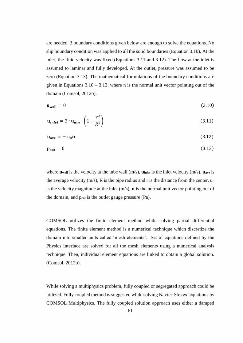
61

are needed. 3 boundary conditions given below are enough to solve the equations. No

slip boundary condition was applied to all the solid boundaries (Equation 3.10). At the

inlet, the fluid velocity was fixed (Equations 3.11 and 3.12). The flow at the inlet is

assumed to laminar and fully developed. At the outlet, pressure was assumed to be

zero (Equation 3.13). The mathematical formulations of the boundary conditions are

given in Equations 3.10 – 3.13, where n is the normal unit vector pointing out of the

domain (Comsol, 2012b).

𝐮𝐰𝐚𝐥𝐥 = 0 (3.10)

𝐮𝒊𝒏𝒍𝒆𝒕 = 2 ∙ 𝐮𝒂𝒗𝒆 ∙ (1 −𝑟2

𝑅2) (3.11)

𝐮𝐚𝐯𝐞 = − u0𝐧 (3.12)

pout = 0 (3.13)

where uwall is the velocity at the tube wall (m/s), uinlet is the inlet velocity (m/s), uave is

the average velocity (m/s), R is the pipe radius and r is the distance from the center, u0

is the velocity magnitude at the inlet (m/s), n is the normal unit vector pointing out of

the domain, and pout is the outlet gauge pressure (Pa).

COMSOL utilizes the finite element method while solving partial differential

equations. The finite element method is a numerical technique which discretize the

domain into smaller units called ‘mesh elements’. Set of equations defined by the

Physics interface are solved for all the mesh elements using a numerical analysis

technique. Then, individual element equations are linked to obtain a global solution.

(Comsol, 2012b).

While solving a multiphysics problem, fully coupled or segregated approach could be

utilized. Fully coupled method is suggested while solving Navier-Stokes’ equations by

COMSOL Multiphysics. The fully coupled solution approach uses either a damped

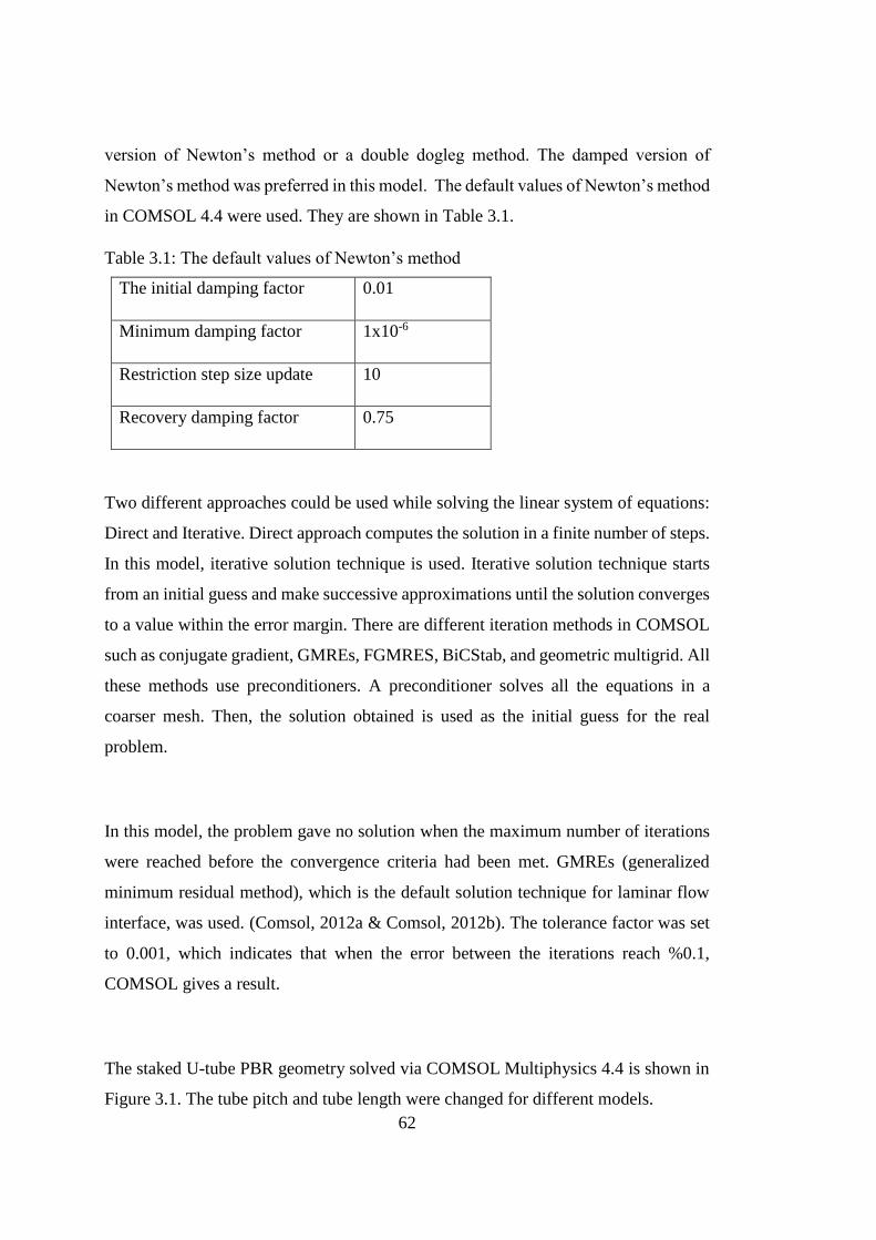
62

version of Newton’s method or a double dogleg method. The damped version of

Newton’s method was preferred in this model. The default values of Newton’s method

in COMSOL 4.4 were used. They are shown in Table 3.1.

Table 3.1: The default values of Newton’s method

The initial damping factor 0.01

Minimum damping factor 1x10-6

Restriction step size update 10

Recovery damping factor 0.75

Two different approaches could be used while solving the linear system of equations:

Direct and Iterative. Direct approach computes the solution in a finite number of steps.

In this model, iterative solution technique is used. Iterative solution technique starts

from an initial guess and make successive approximations until the solution converges

to a value within the error margin. There are different iteration methods in COMSOL

such as conjugate gradient, GMREs, FGMRES, BiCStab, and geometric multigrid. All

these methods use preconditioners. A preconditioner solves all the equations in a

coarser mesh. Then, the solution obtained is used as the initial guess for the real

problem.

In this model, the problem gave no solution when the maximum number of iterations

were reached before the convergence criteria had been met. GMREs (generalized

minimum residual method), which is the default solution technique for laminar flow

interface, was used. (Comsol, 2012a & Comsol, 2012b). The tolerance factor was set

to 0.001, which indicates that when the error between the iterations reach %0.1,

COMSOL gives a result.

The staked U-tube PBR geometry solved via COMSOL Multiphysics 4.4 is shown in

Figure 3.1. The tube pitch and tube length were changed for different models.

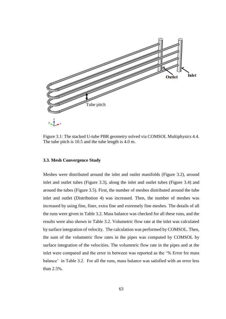
63

Figure 3.1: The stacked U-tube PBR geometry solved via COMSOL Multiphysics 4.4.

The tube pitch is 10.5 and the tube length is 4.0 m.

3.3. Mesh Convergence Study

Meshes were distributed around the inlet and outlet manifolds (Figure 3.2), around

inlet and outlet tubes (Figure 3.3), along the inlet and outlet tubes (Figure 3.4) and

around the tubes (Figure 3.5). First, the number of meshes distributed around the tube

inlet and outlet (Distribution 4) was increased. Then, the number of meshes was

increased by using fine, finer, extra fine and extremely fine meshes. The details of all

the runs were given in Table 3.2. Mass balance was checked for all these runs, and the

results were also shown in Table 3.2. Volumetric flow rate at the inlet was calculated

by surface integration of velocity. The calculation was performed by COMSOL. Then,

the sum of the volumetric flow rates in the pipes was computed by COMSOL by

surface integration of the velocities. The volumetric flow rate in the pipes and at the

inlet were compared and the error in between was reported as the ‘% Error for mass

balance’ in Table 3.2. For all the runs, mass balance was satisfied with an error less

than 2.5%.

Tube pitch

64

Figure 3.2: Twenty meshes distributed around the manifolds (Distribution 1).

Figure 3.3: Twenty meshes distributed around the inlet and outlet pipes (Distribution

2).

65

Figure 3.4: Twenty meshes were distributed along the inlet pipe (Distribution 3).

Figure 3.5: Twenty meshes were distributed around the tubes (Distribution 4).

66

Table 3.2: Details of runs done for the mesh convergence study. The volumetric flow rate was 25 L/h (Ret=92), the tube pitch was

10.5 cm and the tube length was 1.4 m.

Run

no

Distribution

1

Distribution

2

Distribution

3

Distribution

4 Mesh type

Number

of

elements

Average

element

quality

% Error for

the mass

balance

1 20 20 20 10

Extremely

fine 3120192 0.774 0.65

2 20 20 20 10 Extra fine 1147689 0.767 1.37

3 20 20 20 10 Finer 677020 0.770 1.34

4 20 20 20 10 Fine 429589 0.759 3.03

5 20 20 20 20

Extremely

fine 4830079 0.773 0.64

6 20 20 20 20 Extra fine 2043152 0.769 1.35

7 20 20 20 20 Finer 1311929 0.770 1.40

8 20 20 20 20 Fine 839940 0.763 2.21

9 20 20 20 30

Extremely

fine 7251606 0.773 0.82

10 20 20 20 30 Extra fine 3160800 0.770 1.37

11 20 20 20 30 Finer 2070471 0.770 1.29

12 20 20 20 30 Fine 1316951 0.764 2.03

13 5 5 5 5

Extremely

fine 2600023 0.774 0.48

14 5 5 5 5 Extra fine 609805 0.767 0.89

66

67

A mesh convergence study was carried out by comparing the velocities in all the tubes

separately. The volumetric flow rates in different tubes were compared and reported

in

Table 3.3. While calculating the volumetric flow rate, the velocity data computed by

the program was exported. Then, the volumetric flow rate was calculated as shown in

Equation 3.14. For the numerical integration, trapezoidal rule for non-uniform grid

was utilized.

𝑄 = ∫ ∫ 𝑉𝑧𝑟𝑑𝑟𝑑𝜃𝑅

0

2𝜋

0

(3.14)

where Q is the volumetric flow rate, Vz is the velocity in the z direction, r is the distance

from the center, θ is the angle and R is the radius of the tube.

The difference between the extra fine and extremely fine mesh was below 5% for all

the runs with different distribution of meshes. Therefore, extra fine mesh was selected

for further studies.

For all the runs, volumetric flow rate was 25 L/h (Ret=92). When the volumetric flow

rate was increased, COMSOL was not able to find a solution when the distributed

number of meshes exceeds 5. The reason behind this problem was about the solution

technique that the COMSOL utilizes. As the more mesh elements were distributed, the

preconditioner cannot coarsen the mesh. Therefore, the number of mesh elements were

restricted to 5 so that the preconditioner converges and the program finds a solution.

The difference in volumetric flow rates between the Run 10 and Run 14 was found to

be less than 3%, indicating that the reduction in the number of meshes from 30 to 5 in

the distribution 4 did not affected the result significantly. It can be concluded that

distribution 5 was a proper choice for further studies.

68

The model was solved with a mesh number of 609805. The total difference was found

to be less than 5% when the mesh number was increased from 609805 to 2600023.

Table 3.3: Results of mesh convergence study

Pipe

no

Volumetric flow rate (x106 m3/s)

Percent Error Extrem

ely fine

Extra

fine Finer Fine

Distribution 4 = 10

Run 1 Run 2 Run 3 Run 4

Run 1-

Run 2

Run 2 -

Run 3

Run 3 -

Run 4

1 1.90 1.95 1.83 1.79 2.6 6.2 2.7

2 1.89 1.85 1.81 1.80 1.9 2.6 0.2

3 1.84 1.82 1.79 1.70 1.2 1.2 5.3

4 1.83 1.79 1.74 1.66 1.9 3.4 4.8

Distribution 4 = 20


Run 5 -

Run 6

Run 6 -

Run 7

Run 7-

Run 8

1 1.99 1.91 1.88 1.66 4.1 1.7 13.7

2 1.86 1.85 1.76 1.76 0.4 5.3 0.1

3 1.80 1.84 1.74 1.69 2.1 5.7 2.9

4 1.79 1.81 1.73 1.66 1.5 4.8 4.0

Distribution 4 = 30


Run 9 -

Run 10

Run10-

Run11

Run 11-

Run 12

1 1.94 1.96 1.88 1.80 1.4 4.6 4.2

2 1.87 1.83 1.78 1.80 2.2 2.6 0.8

3 1.83 1.80 1.77 1.74 1.4 1.6 2.3

4 1.81 1.78 1.74 1.57 1.7 2.3 10.3

Distribution 4 = 5

Run 13 Run 14

Run13

-Run14

Run 9-

Run 13

Run 10-

Run 14

1 1.88 1.83 3.0 5.9 2.9

2 1.82 1.76 3.6 6.3 2.6

3 1.79 1.74 3.0 5.3 2.3

4 1.77 1.73 2.7 4.7 2.0

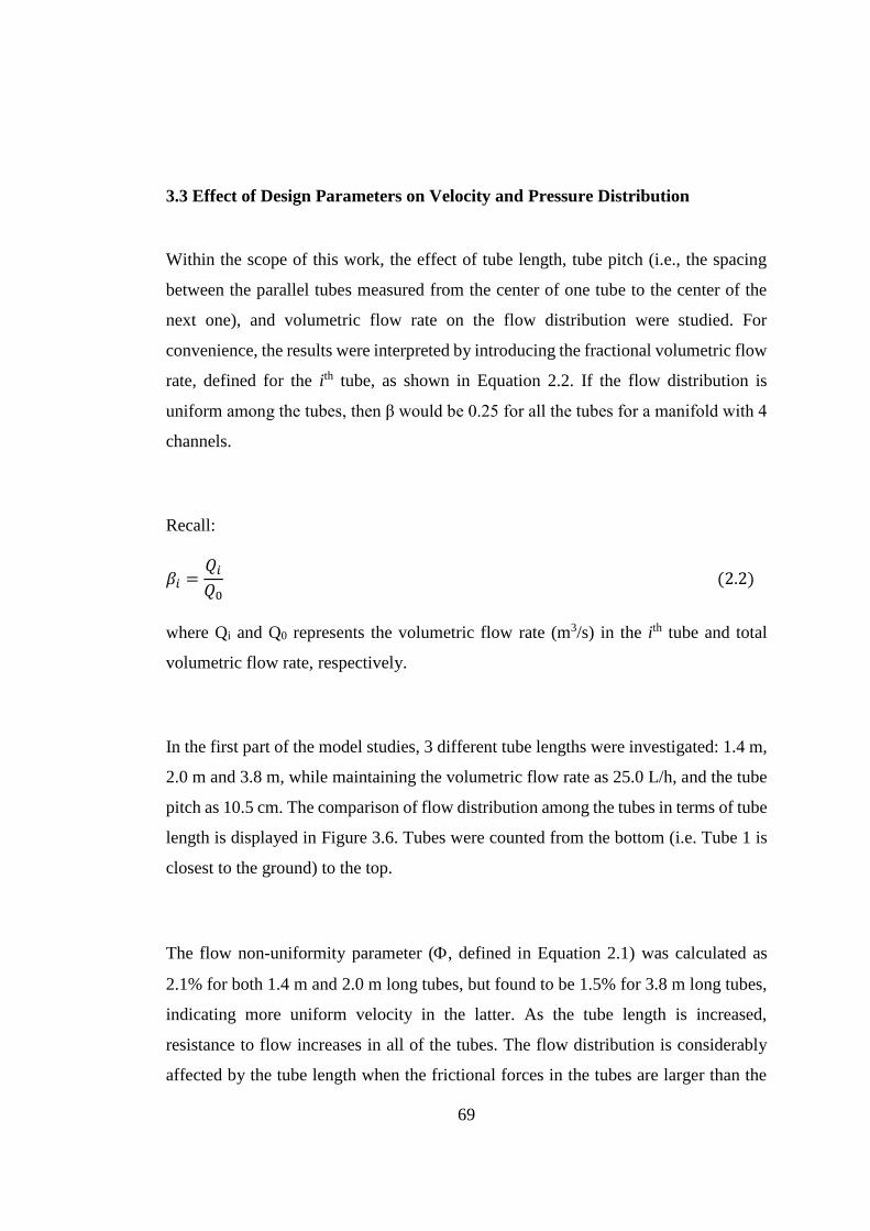
69

3.3 Effect of Design Parameters on Velocity and Pressure Distribution

Within the scope of this work, the effect of tube length, tube pitch (i.e., the spacing

between the parallel tubes measured from the center of one tube to the center of the

next one), and volumetric flow rate on the flow distribution were studied. For

convenience, the results were interpreted by introducing the fractional volumetric flow

rate, defined for the ith tube, as shown in Equation 2.2. If the flow distribution is

uniform among the tubes, then β would be 0.25 for all the tubes for a manifold with 4

channels.

Recall:

𝛽𝑖 =𝑄𝑖

𝑄0 (2.2)

where Qi and Q0 represents the volumetric flow rate (m3/s) in the ith tube and total

volumetric flow rate, respectively.

In the first part of the model studies, 3 different tube lengths were investigated: 1.4 m,

2.0 m and 3.8 m, while maintaining the volumetric flow rate as 25.0 L/h, and the tube

pitch as 10.5 cm. The comparison of flow distribution among the tubes in terms of tube

length is displayed in Figure 3.6. Tubes were counted from the bottom (i.e. Tube 1 is

closest to the ground) to the top.

The flow non-uniformity parameter (, defined in Equation 2.1) was calculated as

2.1% for both 1.4 m and 2.0 m long tubes, but found to be 1.5% for 3.8 m long tubes,

indicating more uniform velocity in the latter. As the tube length is increased,

resistance to flow increases in all of the tubes. The flow distribution is considerably

affected by the tube length when the frictional forces in the tubes are larger than the

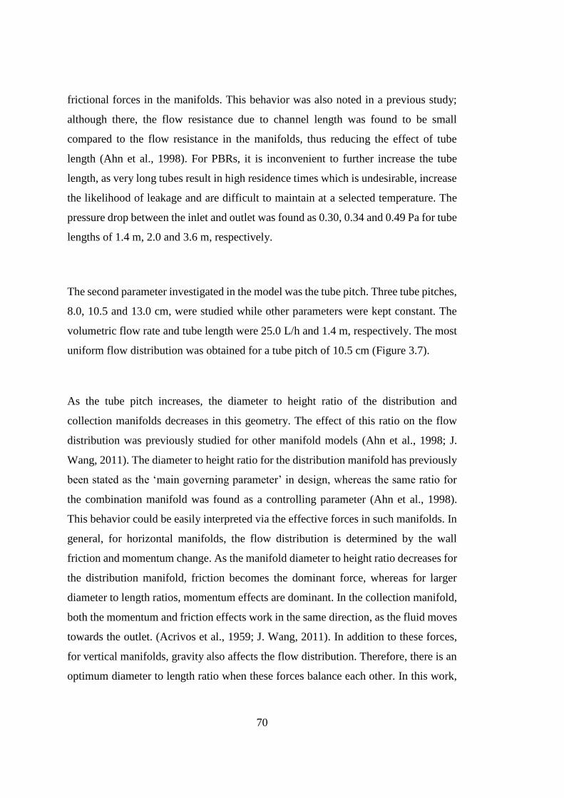
70

frictional forces in the manifolds. This behavior was also noted in a previous study;

although there, the flow resistance due to channel length was found to be small

compared to the flow resistance in the manifolds, thus reducing the effect of tube

length (Ahn et al., 1998). For PBRs, it is inconvenient to further increase the tube

length, as very long tubes result in high residence times which is undesirable, increase

the likelihood of leakage and are difficult to maintain at a selected temperature. The

pressure drop between the inlet and outlet was found as 0.30, 0.34 and 0.49 Pa for tube

lengths of 1.4 m, 2.0 and 3.6 m, respectively.

The second parameter investigated in the model was the tube pitch. Three tube pitches,

8.0, 10.5 and 13.0 cm, were studied while other parameters were kept constant. The

volumetric flow rate and tube length were 25.0 L/h and 1.4 m, respectively. The most

uniform flow distribution was obtained for a tube pitch of 10.5 cm (Figure 3.7).

As the tube pitch increases, the diameter to height ratio of the distribution and

collection manifolds decreases in this geometry. The effect of this ratio on the flow

distribution was previously studied for other manifold models (Ahn et al., 1998; J.

Wang, 2011). The diameter to height ratio for the distribution manifold has previously

been stated as the ‘main governing parameter’ in design, whereas the same ratio for

the combination manifold was found as a controlling parameter (Ahn et al., 1998).

This behavior could be easily interpreted via the effective forces in such manifolds. In

general, for horizontal manifolds, the flow distribution is determined by the wall

friction and momentum change. As the manifold diameter to height ratio decreases for

the distribution manifold, friction becomes the dominant force, whereas for larger

diameter to length ratios, momentum effects are dominant. In the collection manifold,

both the momentum and friction effects work in the same direction, as the fluid moves

towards the outlet. (Acrivos et al., 1959; J. Wang, 2011). In addition to these forces,

for vertical manifolds, gravity also affects the flow distribution. Therefore, there is an

optimum diameter to length ratio when these forces balance each other. In this work,

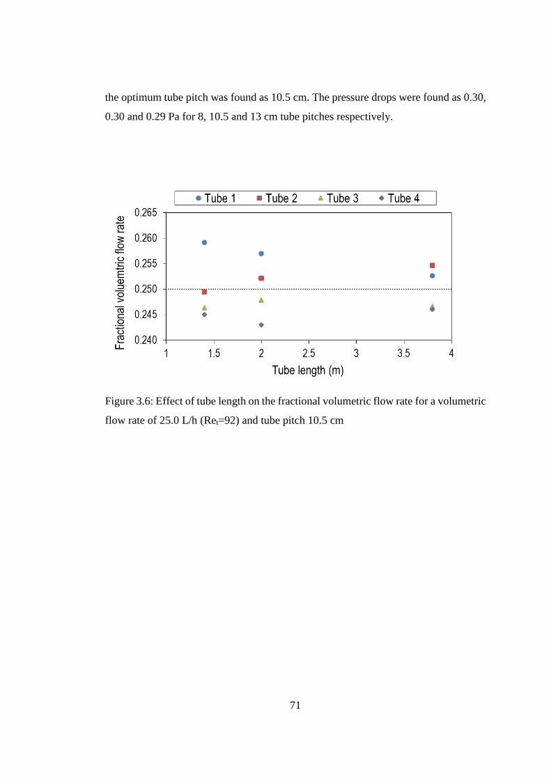
71

the optimum tube pitch was found as 10.5 cm. The pressure drops were found as 0.30,

0.30 and 0.29 Pa for 8, 10.5 and 13 cm tube pitches respectively.

Figure 3.6: Effect of tube length on the fractional volumetric flow rate for a volumetric

flow rate of 25.0 L/h (Ret=92) and tube pitch 10.5 cm

72

Figure 3.7: Effect of tube pitch for a volumetric flow rate of 25.0 L/h and a tube length

of 1.4 m

The volumetric flow rate was increased from 25 L/h to 250 L/h with 25 L/h increments.

For these cases, the tube pitch was 10.5 cm and tube length was 1.4 m. It is more

convenient to report the volumetric flow rates in terms of Reynolds number (Equation

3.14).

Du Re (3.14)

where is the density (kg/m3), u is the velocity (m/s), D is the diameter (m), and

is the viscosity (Pa.s)

In this study, fractional volumetric flow rate was compared using the tube Reynolds

number, Ret. It should be noted that Ret is not the actual Reynolds number in the tubes

computed from the model, but rather a hypothetical number, that gives a sense about

what would have been the Reynolds number in the tubes if the flow was distributed

uniformly to all the tubes.

73

Figure 3.8 indicates that increasing the volumetric flow rate (Ret) did not change the

flow distribution. More fluid tended to go from the lowest tube for all the volumetric

flow rates. This result revealed that both gravitational and momentum effects were

higher compared to frictional effects in the distribution manifold. Still, looking at the

the flow non-uniformity parameter changing between 2.1% and 2.3% for different

flow rates, it could be concluded that a uniform flow distribution was achieved.

Figure 3.8: Effect of fractional volumetric flow rates for tube pitch and tube lengths of

10.5 and 1.4 m, respectively.

Figure 3.9: Pressure drop with respect to volumetric flow rate. The tube pitch and

lengths are 10.5 cm and 1.4 m.

74

The pressure difference between the inlet and outlet of the reactor with respect to Ret

is plotted in Figure 3.9. The pressure drop increased as Ret increased, as expected. The

values were low; however, even for the highest volumetric flow rate (250 L/h) for

which the pressure difference between the inlet and outlet of the reactor was only 20.3

Pa. The summary of the parameters studies are shown in Table 3.4.

Table 3.4: The summary of the parameters studied and corresponding non-uniformity

parameter.

Tube length

(m)

Tube pitch

(cm)

Overall

volumetric flow

rate (L/h)

Ret

Φ (%)

1.4 10.5 25.0 92.0 2.1

2.0 10.5 25.0 92.0 2.1

3.8 10.5 25.0 92.0 1.5

1.4 8 25.0 92.0 2.1

1.4 13 25.0 92.0 3.1

1.4 10.5 50.0 184.0 2.2

1.4 10.5 75.0 276.0 2.2

1.4 10.5 100.0 368.0 2.2

1.4 10.5 125.0 460.0 2.3

1.4 10.5 150.0 552.0 2.3

1.4 10.5 175.0 644.0 2.3

1.4 10.5 200.0 736.0 2.3

1.4 10.5 225.0 828.0 2.3

1.4 10.5 250.0 920.0 2.3

3.4 Evaluation and Final Selection

The issues related with the design discussed above are summarized below:

Tubular reactors are more advantageous due to ease of mixing and cooling.

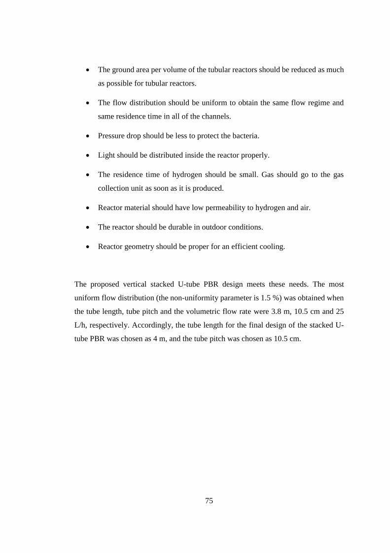
75

The ground area per volume of the tubular reactors should be reduced as much

as possible for tubular reactors.

The flow distribution should be uniform to obtain the same flow regime and

same residence time in all of the channels.

Pressure drop should be less to protect the bacteria.

Light should be distributed inside the reactor properly.

The residence time of hydrogen should be small. Gas should go to the gas

collection unit as soon as it is produced.

Reactor material should have low permeability to hydrogen and air.

The reactor should be durable in outdoor conditions.

Reactor geometry should be proper for an efficient cooling.

The proposed vertical stacked U-tube PBR design meets these needs. The most

uniform flow distribution (the non-uniformity parameter is 1.5 %) was obtained when

the tube length, tube pitch and the volumetric flow rate were 3.8 m, 10.5 cm and 25

L/h, respectively. Accordingly, the tube length for the final design of the stacked U-

tube PBR was chosen as 4 m, and the tube pitch was chosen as 10.5 cm.

77

CHAPTER 4

CONSTRUCTION AND OPERATION

4.1 Materials and Methods

4.1.1 The Bacterial Strain

Rhodobacter capsulatus YO3 (hup-) strain, previously mutated from the wild-type by

Dr. Yavuz Öztürk (GMBE, TUBITAK MAM-Gebze) by deleting the gene coding for

uptake hydrogenase enzyme (hup-) of Rhodobacter capsulatus MT1131 (Öztürk et

al., 2006) was used in this study.

4.1.2 Culture Media

4.1.2.1 Solid Media

Bacteria kept at -80 ºC were activated using a solid media. Solid media were also used

to detect contamination. While preparing solid media, agar (3% w/v) was added to the

growth media. After the media was autoclaved and cooled to around 40 ºC, it was

poured into the agar plates. After solidification of the media, bacteria were inoculated

to the agar plates. The plates were wrapped by an aluminum foil to keep them dark,

and they were kept in an incubator at 30 ºC until visible colonies were obtained.

4.1.2.2 Growth Media

The Biebl and Pfennig (1981) medium containing 20 mM acetate and 10 mM

glutamate as carbon and nitrogen sources respectively, was used for bacterial growth

(Biebl & Pfennig, 1981). After all chemicals were dissolved in distilled water, pH was

78

adjusted to 6.4 – 6.5 by using NaOH solution. The medium was autoclaved for 20

minutes at 121 ⁰C (Prior Clave). After the medium was cooled to room temperature,

trace elements, iron citrate and vitamin solutions were added to the medium in a sterile

cabin. The detailed recipes of the BP medium, trace elements, iron citrate and vitamin

solutions are given in Appendix A.

4.1.2.3 Sucrose Adaptation Media

Bacteria need to be adapted to sucrose before being inoculated to the hydrogen

production media. Therefore, the bacteria were transferred to a sucrose adaptation

medium containing 20 mM acetate, 10 mM glutamate and 5 mM sucrose besides Biebl

and Pfennig (1981). The bacteria stayed in sucrose adaptation media until its OD

reached 1.0 – 1.5 at 660 nm. Then, bacteria were transferred to a second sucrose

adaptation media which contains 5 mM sucrose, 10 mM glutamate and the Biebl and

Pfennig (1981) medium.

4.1.2.4 Hydrogen Production Media Containing Molasses

Molasses bought from Ankara sugar factory was used as the hydrogen production

medium. In this work 5 mM sucrose containing molasses was used as the hydrogen

production medium. In order to control pH, 30 mM KH2PO4 solution was used as

buffer. Initial pH was adjusted to 7.5 with 5 M NaOH solution. After preparing the

buffer solution, molasses was added. 10 % (v/v) bacteria were inoculated to the

hydrogen production medium. In RUN 092014, Fe and Mo were not added. However,

in RUN 072015-R2, Fe and Mo were added to the molasses so that the final amount

of Fe and Mo in the feedstock was 0.1 mM and 0.16 μM, respectively.

79

4.1.2.5 Defined Hydrogen Production Medium

Bacteria which were grown in BP medium containing 40 mM acetate and 20 mM

glutamate medium were transferred to hydrogen production medium which contained

40 mM acetate, 2 mM glutamate and Biebl and Phennig medium. The initial

concentration was adjusted to OD660 of 0.55-0.65. As a buffer, 22mM KH2PO4 was

used. The initial pH was adjusted to 6.3-6.4 by 5 mM NaOH addition.

4.1.2.6. Preparation of Inoculum

First, one colony of bacteria was inoculated to the 1.5 ml growth media. After the OD

value reached to 1.0 – 1.5 at 660 nm, 1.5 ml bacteria was inoculated to 15 ml growth

media. Anaerobic conditions were obtained by flushing the media with argon (99.9 %

purity) for 2 minutes. Then, the same procedure (10 %, v/v inoculation of bacteria)

was applied until the desired amount of culture was obtained.

4.1.2.6 Storage

For long term storage of the bacteria, the medium was mixed with sterile glycerol (40

% v/v) and put into cryogenic vials. The vials were stored in -80 ºC refrigerator. To

store the bacteria for about a mount, the bacteria grown in Biebl and Pfennig (1981)

medium containing 20 mM acetate and 10 mM glutamate was kept at +4ºC in a

refrigerator. The bacteria kept in +4 ºC were activated before use.

4.1.3. Analyses

4.1.3.1.Molasses Analyses

Density and sugar content of molasses together with analysis of some elements (Na,

K, Ca, Mg, Fe, Mn and Zn) were reported by Ankara Sugar Factory, Turkey. The

80

results provided by Ankara Sugar Factory are shown in Table B.1 in Appendix B. Total

amino acids and minerals (Fe, Mo, S, K) were analyzed by Düzen Norwest Laboratory,

Ankara, Turkey. The results of the analysis are given in Table B.2 and Table B.3,

respectively. Amino acids and sucrose are the sources of nitrogen and carbon in

molasses, respectively. Moreover, the necessary nutrients for bacterial growth such as

Fe and Mo are also present in molasses. However, since the molasses needs to be

diluted to adjust the sucrose content, glutamate, Fe and Mo need to be added to obtain

the desired amounts necessary for bacterial growth.

4.1.3.2.Sugar Content Analysis

The sugar content in the samples was analyzed by two different methods. (only sucrose

is expected to be present in the molasses.) In RUN 092015, sucrose was analyzed using

a sucrose kit, provided by Megazyme (Sucrose D-Glucose Assay Kit). The calibration

of the sucrose kit was done by using standard solution. -The samples were filtered with

22 μm filters. In RUN 072015, the sucrose content in the samples was measured by

HPLC (Shimadzu 20A series). Two detectors (UV and RI) were connected in series.

The sucrose content was determined from the results of the RID detector. The column

was Alltech IOA-1000 (300 mm x 7.8 mm). 0.0085 M H2SO4 was used as the mobile

phase. The oven temperature was kept at 60 ºC. A low gradient pump (Shimadzu LC-

20AT) with a degasser (Shimadzu DGU-20A5) was used to keep the flow rate at 0.4

ml/min. 10 μL samples were injected to the system with the help of an auto sampler

(Shimadzu SIL-10AC). RI (refractive index) detector (Shimadzu RID-20A) was used

to determine sugar content. The retention times and peak areas were recorded

automatically. Calibration was done using the standard solutions.

4.1.3.3.Organic Acid Analysis

Organic acids were analyzed by an HPLC (Shimadzu 20A series). The method used

was the same as the method used for sugar content analysis with HPLC except for the

81

detector type. A UV detector (Shimadzu SPD-20A) whose absorbance set at 210 nm

was used for the detection of organic acids. The calibration was done by using standard

solutions for organic acids. Lactic acid, acetic acid, propionic acid and butyric acid

were the organic acids measured.

4.1.3.4. pH Analyses

The pH of the samples was measured with a pH meter (Ezdo MP-103). Three

measurements were taken from each sample and an average was reported. Before

usage, the pH of the standard solutions was measured. If the accuracy was less than

95%, pH meter was calibrated.

4.1.3.5.Cell Concentration

The cell concentration was measured by a UV spectrophotometer (Shimadzu UV-

1201). The absorbance was set at 660 nm. Distilled water was used as a blank solution.

The dry cell weights were determined from absorbance values. The calibration factor

was 0.4656 for Rhodobacter capsulatus YO3 (Öztürk, 2005).

4.1.3.6.Light Intensity

Light intensity was measured with a luxmeter (Lutron LX-105 Light Meter) for

indoors. The PBRs which were kept in an incubator (Nüve) was illuminated by 100 W

tungsten lamps. The light intensity on the surface of the PBRs was adjusted to 2000

lux.

The light intensity for RUN 092014 was recorded by a pyranometer (HOBO-S-LIB-

M003) which was connected to an online weather station (HOBO® U30 ETH).

82

The light intensity values were recorded for RUN 072015-R1 and RUN072015-R2 by

a weather station (Davis Vantage Pro2 Weather Station equipped with a solar radiation

sensor) which was mounted near the reactors.

4.1.3.7.Temperature Measurements

The temperature measurements were taken with thermocouples (Fe-constant J type)

which are connected to an online data logger (Ordel UDL100). 12 temperature

measurements were taken from RUN 092014 and RUN 072015-R1. The ports in which

thermocouples were inserted are shown in Figure 4.6. For RUN 092014, cooling water

inlet and outlet temperatures were also measured. 2 temperature measurements were

taken from RUN 072015-R2 (T4 and T12). Air temperature was also measured with J

type thermocouple for RUN 092014. Air temperature data for RUN 072014-R1 and

RUN 072014-R2 were measured by the weather station (Davis Vantage Pro2 Weather

Station).

4.1.3.8.Gas Analysis

The gas composition was determined by using a gas chromatography (Agilent

Technologies 6890N) equipped with a Supelco Carboxen 1010 column. A thermal

conductivity detector was used. 100 μL samples were injected to the gas

chromatography with a gas-tight syringe (Hamilton, 22 GA 500μL). Argon was used

as the carrier gas. The flow rate of Argon gas was 26 mL/min. The oven, injector and

detector temperatures were 140, 160 and 170 ºC, respectively.

4.2 Construction

The hydrodynamic model of the PBR was developed and shown in ‘Modelling of

Photobioreactor’. The pilot scale reactor was constructed based on the dimensions

83

obtained from the model. The PBR was made of glass. The details of the PBR

dimensions are given below.

4.2.1 Inlet and Outlet Manifolds

The fluid was distributed to the tubes by means of manifolds. Inlet and outlet manifolds

were identical. They are made of glass. The diameter of each manifold was 6 cm, and

the length was 47.5 cm. The wall thickness of the glass manifolds was 2 mm. At the

upper side of the manifold, gas was collected by connecting a polyurethane pipe to the

manifold. The inlet manifold has one inlet which has 12 cm diameter, 4 exits with 3

cm outside diameters and a gas exit whose outside diameter was 6 mm. Similarly, the

outlet manifold has 4 inlets with 3 cm diameters, 1 outlet which has 18 cm diameter,

and 1 gas outlet with 6 mm outside diameter.

In order to keep the temperature of the reactor at the desired values, a spiral glass

cooling coil was designed inside the manifolds. Temperature was measured at the

bottom and upper side of the manifold by inserting J-type thermocouples. The inlet

and outlet manifolds were shown in Figure 4.1.

84

(a) (b)

Figure 4.1: Inlet and Outlet manifolds (a) front view (b) side view

4.2.2 Tubing

Hydrogen production mainly occurred in the glass tubes. Glass tubes have 3 main

sections for the ease of use. 2 tubes with 1.5 m in length were connected to manifolds.

U – Tube was used to connect these tubes (Figure 4.2-a). Tees were used for sampling

as shown in Figure 4.2-b. The tube diameter was chosen as 3 cm after the experiments

mentioned in Diameter Selection (Appendix C) were performed. The wall thickness

of the tubes was chosen as 1.5 mm. Hydrogen production mainly occurred in this part

of the reactor. Temperature was measured in the reactor at 3 points by using tees: after

the inlet manifold, before U – tube and before outlet manifold. U-tubes were tilted 30

ºC in order to collect the hydrogen gas easily. Connections of the glass tubes were

made via silicon pipe.

85

(a) (b)

Figure 4.2: a) U – tubes b) Tees for sampling and thermocouples

Polyurethane pipes, which have 5.5 mm inlet diameter and 8 mm outlet diameter, were

used between the gas outlet of the manifolds and the gas collection unit.

To provide a secondary cooling capability (in addition to the glass coils in the

manifolds) PVC cooling pipes were inserted into each of tube during RUN 092014 in

order to keep the temperature of the reactor below 40 ºC in summer. The pipes had an

inner diameter of 5 mm and an outer diameter of 7 mm. These pipes were connected

to a process water cooler (PNÖSO PSS 6 D). The cooling water temperature ranged

between 5 – 10 ºC manually, in order to keep the temperature of the reactor below 40

ºC in summer.

86

No cooling coils were inserted into the tubes during RUN 072015-R1 and RUN

082015-R2. The temperature was controlled by using a controller system which

changed the flow rate of the cooling water to keep the reactor temperature at 30ºC.

4.2.3 Stand

A stand was designed for the PBR by taking into account the approximate weight of

the PBR. Inlet and outlet manifolds were put on a metal sheet that was welded on the

stand. The inlet manifold stands 30 cm above ground whereas outlet manifold stands

on the 38 cm above ground so that U-tubes would be 30ºC tilted. The pipes were

fastened with pipe clamps. Wheels were fitted to the stand for ease of movement.

4.3 Pump Selection

It is generally argued that the bacteria cannot stand high shear stresses in pumping and

recirculation (Flickinger, 2013; Li et al., 2011). Therefore, the pressure difference

created by the pump could become an important parameter in large scale operations.

In order to understand the effect of pump type, an experiment was carried out. U-tube

PBRs were run parallel with Rhodobacter Capsulatus YO3. 5 mM sucrose-containing

molasses was used as the hydrogen production medium. The experimental set-up is

shown in Figure 4.3.

The growth of the bacteria was compared in two U-tube parallel reactors whose

volumes were 3 L. One of the reactors was operated with a centrifugal aquarium pump

(referred to simply as the aquarium pump henceforth); whereas the other was operated

with a peristaltic pump. A higher biomass concentration was achieved with the

peristaltic pump on the first day (Figure 4.1). However, for rest of the 3-day

experiment, the order of biomass concentrations in both of the systems became the

same (Figure 4.5).

87

Figure 4.3: U-tube PBRs operated with an aquarium pump (left) and a peristaltic pump

(right). The experiment started on December 28, 2014 and lasted 3 days.

While growth was observed to be more or less the same, the peristaltic pump was

observed to have several practical advantages over the aquarium pump. It is easy to

adjust the flow rate with the peristaltic pump. While the centrifugal pump requires a

recycle loop to reduce the flow rates to the targeted Reynolds range, this need is

eliminated when a peristaltic pump is used; therefore, there is no need for extra

connections. The number of connections in the pilot system should be as few as

possible, since every connection brings about a potential leakage problem. Besides,

most of the connections are metal in the centrifugal pump, which could affect bacterial

growth and hydrogen production (Avcioglu, 2010), whereas peristaltic pump parts do

not come directly into contact with the culture medium. Based on these considerations,

the peristaltic pump was selected as the suitable pump type for photofermentative

hydrogen production. Details of the experimental procedure and the experimental data

obtained during the comparison of the pump types are given in Appendix D.

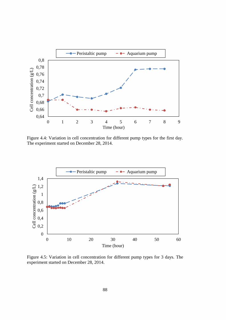
88

Figure 4.4: Variation in cell concentration for different pump types for the first day.

The experiment started on December 28, 2014.

Figure 4.5: Variation in cell concentration for different pump types for 3 days. The

experiment started on December 28, 2014.

0,64

0,66

0,68

0,7

0,72

0,74

0,76

0,78

0,8

0 1 2 3 4 5 6 7 8 9

Cel

l co

nce

ntr

atio

n (

g/L

)

Time (hour)

Peristaltic pump Aquarium pump

0

0,2

0,4

0,6

0,8

1

1,2

1,4

0 10 20 30 40 50 60

Cel

l co

nce

ntr

atio

n (

g/L

)

Time (hour)


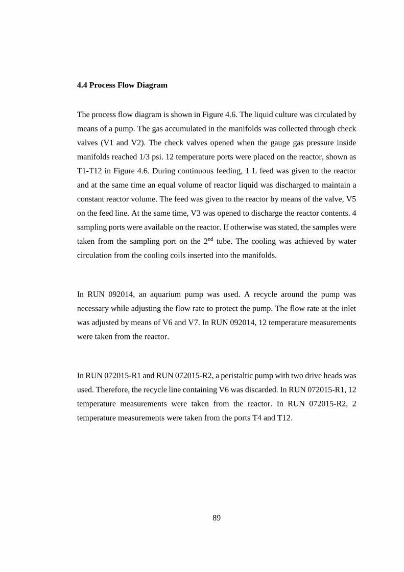
89

4.4 Process Flow Diagram

The process flow diagram is shown in Figure 4.6. The liquid culture was circulated by

means of a pump. The gas accumulated in the manifolds was collected through check

valves (V1 and V2). The check valves opened when the gauge gas pressure inside

manifolds reached 1/3 psi. 12 temperature ports were placed on the reactor, shown as

T1-T12 in Figure 4.6. During continuous feeding, 1 L feed was given to the reactor

and at the same time an equal volume of reactor liquid was discharged to maintain a

constant reactor volume. The feed was given to the reactor by means of the valve, V5

on the feed line. At the same time, V3 was opened to discharge the reactor contents. 4

sampling ports were available on the reactor. If otherwise was stated, the samples were

taken from the sampling port on the 2nd tube. The cooling was achieved by water

circulation from the cooling coils inserted into the manifolds.

In RUN 092014, an aquarium pump was used. A recycle around the pump was

necessary while adjusting the flow rate to protect the pump. The flow rate at the inlet

was adjusted by means of V6 and V7. In RUN 092014, 12 temperature measurements

were taken from the reactor.

In RUN 072015-R1 and RUN 072015-R2, a peristaltic pump with two drive heads was

used. Therefore, the recycle line containing V6 was discarded. In RUN 072015-R1, 12

temperature measurements were taken from the reactor. In RUN 072015-R2, 2

temperature measurements were taken from the ports T4 and T12.

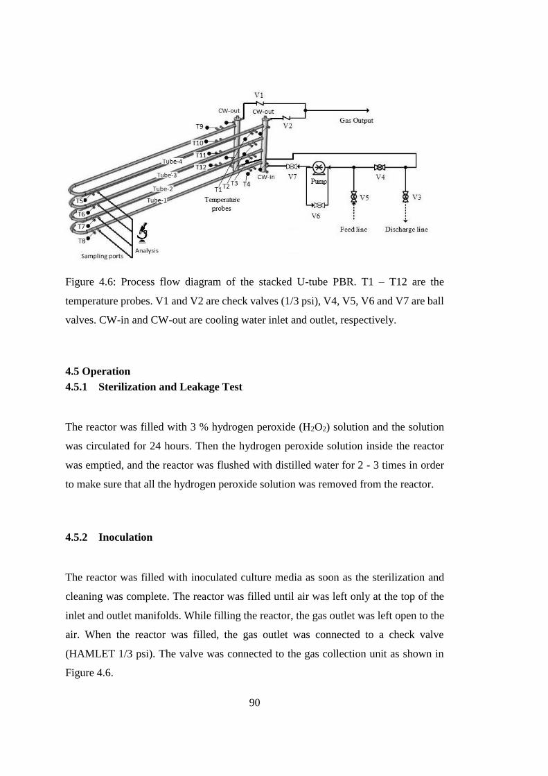
90

Figure 4.6: Process flow diagram of the stacked U-tube PBR. T1 – T12 are the

temperature probes. V1 and V2 are check valves (1/3 psi), V4, V5, V6 and V7 are ball

valves. CW-in and CW-out are cooling water inlet and outlet, respectively.

4.5 Operation

4.5.1 Sterilization and Leakage Test

The reactor was filled with 3 % hydrogen peroxide (H2O2) solution and the solution

was circulated for 24 hours. Then the hydrogen peroxide solution inside the reactor

was emptied, and the reactor was flushed with distilled water for 2 - 3 times in order

to make sure that all the hydrogen peroxide solution was removed from the reactor.

4.5.2 Inoculation

The reactor was filled with inoculated culture media as soon as the sterilization and

cleaning was complete. The reactor was filled until air was left only at the top of the

inlet and outlet manifolds. While filling the reactor, the gas outlet was left open to the

air. When the reactor was filled, the gas outlet was connected to a check valve

(HAMLET 1/3 psi). The valve was connected to the gas collection unit as shown in

Figure 4.6.

91

4.5.3 Continuous Feeding

In RUN 092015, the feeding started on the 3rd day of the experiment when the bacterial

concentration stabilized. The feeding strategy was modified several times during this

experiment, as discussed in detail in the ‘Results and Discussion’ part. A photograph

taken during RUN 092015 is shown in Figure 4.7.

In RUN 072015-R1 (where acetate was the carbon source), the feeding was started

when the cell density stabilized around an OD660 of 1.5 on the 4th day of the

experiment. The feeding strategy was to keep the acetic acid concentration at 40 mM.

Figure 4.7: A photograph of the experimental set up (RUN 091025). The experiment

performed with R. capsulatus YO3 on molasses.

Each morning, as mentioned previously, 1 L fresh medium was fed in exchange for 1

L of reactor medium discharged. The acetic acid concentration in the feed was adjusted

so that its concentration within the reactor remained around 40 mM. The feed also

contained 2 mM sodium glutamate, vitamins, trace elements and Fe-citrate. The

concentrations of vitamin, trace elements and Fe-citrate solutions were adjusted by

taking into account the amounts added to 1 L basal medium. The contents of the

solutions are given in Appendix A. A picture of the reactor is given as Figure 4.8.

92


on acetic acid (RUN 072015 – R1)

In RUN 072015-R2 (with molasses as the carbon source), the feeding was started on

the 5th day (17.07.2015). Every morning, 1 L of feed containing molasses was fed to

the reactor while 1 L of the reactor contents was discharging. The feeding strategy was

to keep the sucrose concentration at 5 mM in the reactor. The sucrose concentration of

the feed was adjusted accordingly every day. The feed was supplied with molybdenum

(0.16 μM) and iron (0.1 mM) by the addition of sodium molybdate (Na2MoO4.2H2O)

93

and iron (III) citrate (Fe(C6H5O7)). The metal concentrations were based on previous

studies. A photograph of the reactor operated with R. capsulatus on molasses is shown

in Figure 4.9. Another picture showing both reactors (RUN 071025-R1 and RUN

072015-R2) is shown in Figure 4.10.


on molasses (RUN 072015 – R2).

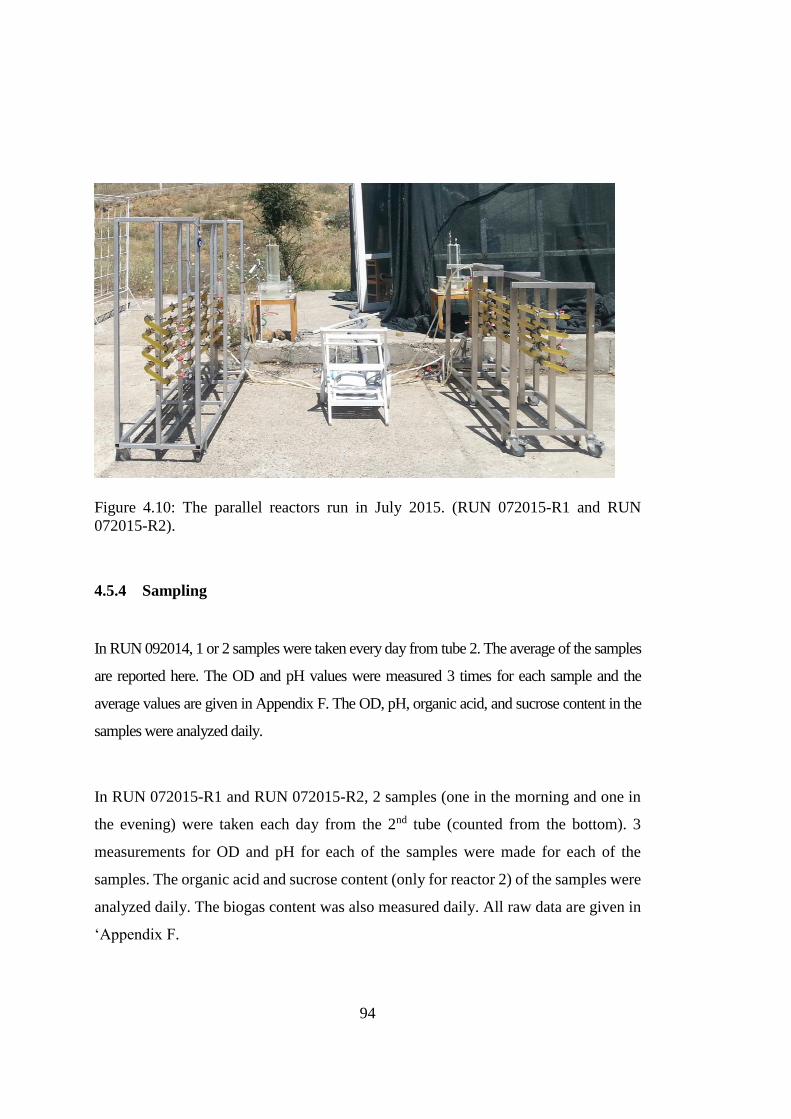
94

Figure 4.10: The parallel reactors run in July 2015. (RUN 072015-R1 and RUN

072015-R2).

4.5.4 Sampling

In RUN 092014, 1 or 2 samples were taken every day from tube 2. The average of the samples

are reported here. The OD and pH values were measured 3 times for each sample and the

average values are given in Appendix F. The OD, pH, organic acid, and sucrose content in the

samples were analyzed daily.

In RUN 072015-R1 and RUN 072015-R2, 2 samples (one in the morning and one in

the evening) were taken each day from the 2nd tube (counted from the bottom). 3

measurements for OD and pH for each of the samples were made for each of the

samples. The organic acid and sucrose content (only for reactor 2) of the samples were

analyzed daily. The biogas content was also measured daily. All raw data are given in

‘Appendix F.

95

CHAPTER 5

RESULTS AND DISCUSSION

5.1 September 2014 Outdoor Experiment with Rhodobacter capsulatus YO3

(hup-) on Molasses (Run 092014)

The experiment with R. capsulatus YO3 was conducted between September 9 and

September 29, 2014. The reactor was cooled intermittently, only on days 2, 3, 4 and

6 at noon time, to keep the culture temperature below 40ºC. The temperature variation

of the culture along the reactor length is shown in Figure 5.1-a. Temperature did not

change significantly along the reactor length when there was cooling. Temperature

variation from tube to tube was also insignificant (Figure 5.1-b). However, as

expected, the lowest temperature was observed in the lowest tube (T12), when cooling

started, since cooling water enters the manifolds from the bottom. The temperature

variation according to tube position and length was not appreciable when there was no

cooling. (Figure 5.2). It can be observed that the reactor temperature followed the same

trend with the air temperature, but it was slightly higher. The daily temperature

variation within the reactor is illustrated in Figure 5.3. As expected, the liquid culture

temperature was highly affected by the solar radiation. Since most of the time there

was no cooling, the temperature of the reactor was mainly driven by solar radiation.

96




the length of the PBR on the 6th day of the experiment. The experiment started on

September 9, 2014. (T9, T10, T11 and T12 were measured from the exit ports of tube

4, tube 3, tube 2 and tube 1, respectively.)

(a)

(b)

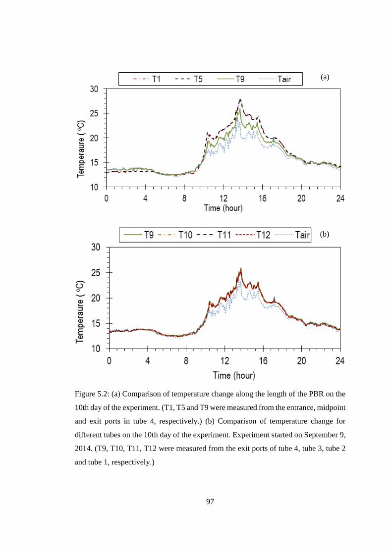
97

Figure 5.2: (a) Comparison of temperature change along the length of the PBR on the

10th day of the experiment. (T1, T5 and T9 were measured from the entrance, midpoint

and exit ports in tube 4, respectively.) (b) Comparison of temperature change for

different tubes on the 10th day of the experiment. Experiment started on September 9,

2014. (T9, T10, T11, T12 were measured from the exit ports of tube 4, tube 3, tube 2

and tube 1, respectively.)

(a)

(b)

98


RUN072015-R1. T9 is measured from the exit port of the tube 4. Experiment started

on September 9, 2014.

The feeding strategy was based on the work of Sağır (2012). The highest hydrogen

production was found with R. capsulatus YO3 with 5 mM sucrose containing molasses

in a batch PBR (Sağır, 2012). However, due to the fact that the observed sucrose

consumption rate of the present study was found to deviate considerably from indoor

results, a more variable strategy had to be adopted based on the culture response in

order to maintain the nutrients and reactor conditions close to optimal conditions. The

‘phases’ of this feeding strategy were given in Table 5.1 and are explained further

below.

The initial sucrose concentration of molasses was adjusted to 5 mM. The cell

concentration stabilized at the 3rd day of the experiment (Phase I) and the sucrose

concentration decreased to very low values (around 0.5 mM). To increase the cell

concentration, Phase II, involving continuous feeding of molasses, was started on the

4th day.

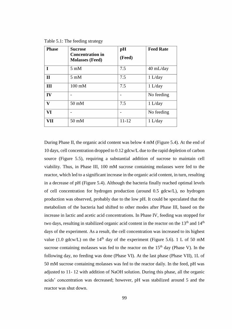
99

Table 5.1: The feeding strategy

Phase Sucrose

Concentration in

Molasses (Feed)

pH

(Feed)

Feed Rate

I 5 mM 7.5 40 mL/day

II 5 mM 7.5 1 L/day

III 100 mM 7.5 1 L/day

IV - - No feeding

V 50 mM 7.5 1 L/day

VI - - No feeding

VII 50 mM 11-12 1 L/day

During Phase II, the organic acid content was below 4 mM (Figure 5.4). At the end of

10 days, cell concentration dropped to 0.12 gdcw/L due to the rapid depletion of carbon

source (Figure 5.5), requiring a substantial addition of sucrose to maintain cell

viability. Thus, in Phase III, 100 mM sucrose containing molasses were fed to the

reactor, which led to a significant increase in the organic acid content, in turn, resulting

in a decrease of pH (Figure 5.4). Although the bacteria finally reached optimal levels

of cell concentration for hydrogen production (around 0.5 gdcw/L), no hydrogen

production was observed, probably due to the low pH. It could be speculated that the

metabolism of the bacteria had shifted to other modes after Phase III, based on the

increase in lactic and acetic acid concentrations. In Phase IV, feeding was stopped for

two days, resulting in stabilized organic acid content in the reactor on the 13th and 14th

days of the experiment. As a result, the cell concentration was increased to its highest

value (1.0 gdcw/L) on the 14th day of the experiment (Figure 5.6). 1 L of 50 mM

sucrose containing molasses was fed to the reactor on the 15th day (Phase V). In the

following day, no feeding was done (Phase VI). At the last phase (Phase VII), 1L of

50 mM sucrose containing molasses was fed to the reactor daily. In the feed, pH was

adjusted to 11- 12 with addition of NaOH solution. During this phase, all the organic

acids’ concentration was decreased; however, pH was stabilized around 5 and the

reactor was shut down.

100

Figure 5.4: Organic acid and pH variation in the reactor. Experiment started on

September 9, 2014.

Figure 5.5: Daily sucrose concentration change. Daily sucrose concentration change.

Experiment started on September 9, 2014.

101

Figure 5.6: Daily cell concentration change. Experiment started on September 9, 2014.

5.2 July 2015 Outdoor Experiments with Rhodobacter capsulatus YO3 (hup-)

(Run 072015)

Two reactors were run in parallel with Rhodobacter capsulatus YO3 (hup-) in July

2015. Reactor 1 (R1) initially contained 40 mM acetic acid and 2 mM sodium

glutamate, whereas Reactor 2 initially contained 5 mM sucrose containing molasses.

Details of the experimental operation of the reactors were given previously under the

‘Operation’ part of Chapter 4.

Both of the reactors were operated at the same recirculation flow rate: 80.4 L/h

(Ret=296) between July 12 and July 16, 2015, and 100 L/h (Ret=368) between July 16

and July 24, 2015. The flow rate was increased at July 16, because cooling was not

sufficient with 80.4 L/h. By increasing the recirculation flow rate, convective cooling

was improved. Besides, the residence time of the culture in the tubes was decreased.

Therefore, the cooling become more effective in the reactor.

A temperature controller was installed to the reactor system to keep the reactor

temperature about 30ºC. The cooling water temperature was set manually between 5

and 10ºC, though it was fixed at 10ºC most of the time. The controller varied the

102

cooling water flow rate to maintain the set point. The temperature of Reactor 1 was

measured from the port T11, and the cooling water flow rate was adjusted accordingly

for both reactors.


(hup-) on Artificial Medium

The experiment with R. capsulatus YO3 was carried on with artificial medium between

July 12 and July 21, 2015. The volume of the reactor (Reactor 1) was 11 L. Both

reactors were cooled solely from the cooling coils inserted into the manifolds. It was

observed that the flow rate of the reactor had an effect on the temperature profile. At

the extreme case, at which flow was completely stopped, the temperature just before

the collection manifold (T9, T10, T11, and T12) would be higher than the air

temperature presumably due to metabolic activity and absorption of radiation. This

behavior was also observed previously in RUN 092014, when there was no cooling

(Figure 5.2). Additionally, the temperature of the tube closer to the ground was

significantly lower than the temperature of higher ones, since the cooling water entered

the manifolds from the bottom. In order to make sure that the reactor was efficiently

cooled, the temperature of the reactor was checked at several locations. The

temperature difference along the reactor length was noted and the corresponding

results are displayed in Figure 5.7-a. Figure 5.7-a indicates that the temperature

gradient was acceptable. The temperature difference along the length of the PBR

remained below 5ºC.

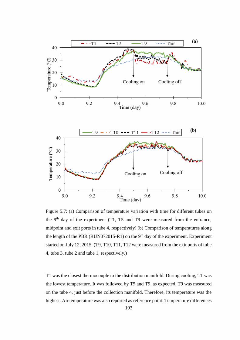
103




the length of the PBR (RUN072015-R1) on the 9th day of the experiment. Experiment

started on July 12, 2015. (T9, T10, T11, T12 were measured from the exit ports of tube

4, tube 3, tube 2 and tube 1, respectively.)

T1 was the closest thermocouple to the distribution manifold. During cooling, T1 was

the lowest temperature. It was followed by T5 and T9, as expected. T9 was measured

on the tube 4, just before the collection manifold. Therefore, its temperature was the

highest. Air temperature was also reported as reference point. Temperature differences

(a)

(b)

104

between the tubes were also compared in Figure 5.7-b. Again, T9 was found as the

highest temperature. There was not a significant temperature gradient between the

tubes. The temperature in all of the tubes (T5, T6, T7 and T8) was maintained around

35ºC. Therefore, an effective cooling was achieved. The changes in reactor (T9) and

the air temperature and solar radiation during the experiment were shown in Figure

5.8.


RUN072015-R1. T9 is measured from the exit port of the tube 4. The experiment was

started on July 12, 2015.

The dry cell weight and hydrogen production was shown in Figure 5.9-a and Figure

5.9-b, respectively. The maximum cell concentration was observed on the 3rd day as

0.748 gdcw/L. After the feeding started on the 4th day, the cell concentration was

stabilized in between 0.5 and 0.6 gdcw/L.

The average hydrogen productivity was found as 0.077 mol H2/(m3.h). The highest

productivity, 0.144 mol H2/(m3.h), was observed on the 2nd day of the experiment

(Figure 5.9). A sample calculation for the productivity is given in Appendix K.1. In

comparison, Boran (2010) performed an outdoor experiment with R. capsulatus YO3

on an artificial medium containing acetate, reporting the average and maximum

105

productivity as 0.20 and 0.40 mol H2/(m3.h), respectively (Boran et al., 2012a). The

feed was not autoclaved in this run to simulate industrial scale applications. However,

this probably caused a decrease in productivity.

Figure 5.9: (a) Variation in cell concentration (b) Daily hydrogen production in

outdoors with R. capsulatus YO3 on artificial medium under non-sterile conditions

(RUN072015-R1).

The starting date of the experiment was July 12, 2015. Feeding started on the 4th day

In Table 5.2, total gas produced and the gas percentages are shown. Substrate

(a)

(b)

106

conversion efficiency and light conversion efficiency are also given in Table 5.2. The

maximum substrate conversion efficiency was found 17.5 % on the 3rd day of the

experiment. The maximum light conversion efficiency was found as 0.027 % on the

2nd day of the experiment. The sample calculations for the substrate conversion

efficiency and the light conversion efficiency are given in Appendix K.2 and K.3,

respectively. The average substrate conversion efficiency was calculated (excluding

the last day) as 9.2%. In another outdoor study, the substrate conversion efficiency was

calculated as 15% when R. capsulatus YO3 on acetic acid was utilized (Boran et al.,

2012b). The maximum substrate conversion efficiency in this study was found higher

than that is found by Boran et al (2012b). When acetic acid in the dark fermenter

effluent of thick juice was utilized with the same bacteria, the substrate conversion

efficiency was found as 9 % (Boran et al., 2012a, 2012b).

Table 5.2: The experimental results of hydrogen in outdoors with R. capsulatus YO3

on artificial medium under non-sterile conditions (RUN072015-R1).

Date

Gas

content

Total

gas

(mL)

H2

productivity

(mol

H2/(m3.h)

Light

conversion

efficiency,

%

H2

%

CO2

%

Substrate

conversion

efficiency %

13.07.2015 96.8 3.2 171 0.038 0.007 5.1

14.07.2015 96.5 3.5 643 0.144 0.027 8.5

15.07.2015 97.6 2.4 372 0.084 0.016 17.5

16.07.2015 95.8 4.2 556 0.123 0.021 12.5

17.07.2015 93.0 7.0 486 0.035 0.006 7.0

18.07.2015 78.7 21.3 239 0.044 0.007 8.3

19.07.2015 87.2 12.8 429 0.087 0.015 8.2

20.07.2015 87.5 12.5 301 0.061 0.010 6.7

21.07.2015 6.5 93.5 2 0.000 0.000 0.0

107


Capsulatus YO3 on artificial medium under non-sterile conditions (RUN072015-R1).

The starting date of the experiment was 12.07.2015. Feeding started on the 4th day.

The variation in organic acid concentration and pH are shown in Figure 5.10. Acetic

acid concentration decreased to around 20 mM during the batch phase. When the

feeding started, acetic acid concentration was adjusted to 40 mM every day in the

morning. Lactic acid, formic acid, propionic acid and butyric acid concentrations

remained under 1 mM (11 mmol). After the continuous feeding started, 2-3 mM (22-

33 mmol) acetic acid was consumed daily. The pH of the culture was between 6.4 and

7.0 throughout the experiment.


(hup-) on Molasses in July

The experiment with R. capsulatus YO3 on molasses (RUN 092014) was repeated

between July 12 and July 24, 2015. The reactor was operated under the same

conditions as RUN 072015-R1. Apart from the medium, the only difference between

the two reactors (R1 and R2) was the volume. R1 was 11 L; whereas R2 was 9 L

because of the difference in their headspaces.

108

The temperature of Reactor 2 (R2) was measured with thermocouples, T4 and T12,

which were both located on the tube closest to the ground (Tube 1). The thermocouple,

T4 was just after the distribution manifold, and T12 was located at the end of the same

tube, just before the collection manifold. The temperature along the tube length for

Reactor 2 did not change significantly (Figure 5.11). Therefore, it can be concluded

that efficient cooling was also achieved in Reactor 2 as in Reactor 1.

In order to have a closer look at the temperature difference between the two reactors,

Figure 5.12 was plotted. The temperatures measured from the thermocouples T12 for

both of the reactors were very similar throughout the experiment.

Daily variations in sucrose concentration for RUN072915-R2 are shown in Figure

5.13. Daily, the sucrose concentration in the reactor was adjusted to 5 mM after the

continuous feeding started. The measurements were taken each day, in the morning

before feeding and in the evening. In the actual case, the sucrose concentration went

as high as 5 mM every day in the morning, and almost all of the sucrose was consumed

daily. In comparison, under indoor conditions the bacteria consumed 47 % of the

sucrose during 200 hours (~8days) (Sağır, 2012). It is obvious that there is a great

difference in the sucrose consumption rate in indoor and outdoor experiments. This

makes it difficult to find a proper feeding strategy, since the sucrose consumption rate

is also related with some of the uncontrolled and fluctuating parameters in outdoors

such as light intensity and temperature. The kinetics of the sucrose consumption rate

and its relation with the light intensity should be investigated further to find the best

feeding strategy.

109


RUN072015-R2. T4 and T12 were measured from after the distribution manifold and

before the combination manifold, respectively. Both of them were on the Tube 1.

Experiment started on July 12, 2015.

Figure 5.12: The comparison of the temperatures for RUN072015-R1 and

RUN072015-R2. R1-T12 and R2-T12 were measured on the Tube 1 just before the

combination manifold. Experiments started on July 12, 2015.

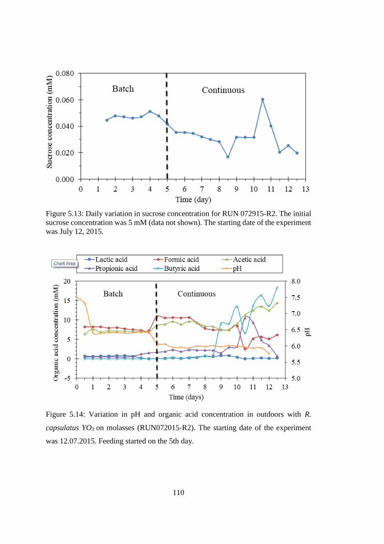
110

Figure 5.13: Daily variation in sucrose concentration for RUN 072915-R2. The initial

sucrose concentration was 5 mM (data not shown). The starting date of the experiment

was July 12, 2015.


capsulatus YO3 on molasses (RUN072015-R2). The starting date of the experiment

was 12.07.2015. Feeding started on the 5th day.

111

The change in the daily organic acid concentration is shown in Figure 5.14. pH

decreased to 5.5 – 6 during the experiment possibly due to the formation of organic

acids. After the continuous feeding started, pH decreased even more. Therefore, on the

6th day, the pH of the feed was increased to 9.0 with NaOH addition. The pH of the

feed was adjusted to 9.0-10.0 for the following days. After the 6th day, the pH of the

culture stabilized around 6.0.

The acetic acid concentration during the entire experiment was in between 5- 15 mM.

When the acetic acid pathway is used, 24 moles of hydrogen should be produced from

one mole of sucrose. The highest substrate conversion efficiency based on these

reactions was determined as 3.7 % on the 10th day of the experiment (Table 5.3)

assuming only the acetic acid pathway was used. The average substrate conversion

efficiency (excluding the days with no hydrogen production) was calculated as 1.9 %.

This is yield is hypothetical, since other organic acids are also produced in the medium.

When the pathway differs, theoretical hydrogen production from 1 mol of sucrose also

differs.

The dry cell weight and hydrogen production was shown in Figure 5.15 and Figure

5.16, respectively. The dry cell weight changed between 0.4 and 0.6 gdcw/L after the

continuous feeding started.

112

Figure 5.15: Cell concentration and hydrogen production in outdoors with R.

Capsulatus YO3 on molasses (RUN072015-R2). The starting date of the experiment

was 12.07.2015.

Figure 5.16: Daily hydrogen productivity. The starting date of the experiment was

12.07.2015.

It is known that the optimum pH for hydrogen production is 7.0. Previous studies show

that hydrogen production diminish at pH 6.0 and completely stops around pH of 5.0

(Sasikala et al., 1991). During this experiment, the hydrogen production continued

even though the pH values got as low as 5.5 - 6.0. The average and the highest

productivities were found as 0.108 mol H2/(m3.h) and 0.311 mol H2/(m

3.h),

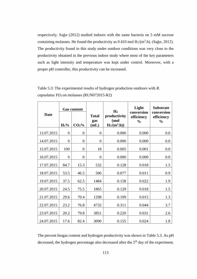
113

respectively. Sağır (2012) studied indoors with the same bacteria on 5 mM sucrose

containing molasses. He found the productivity as 0.410 mol H2/(m3.h). (Sağır, 2012).

The productivity found in this study under outdoor conditions was very close to the

productivity obtained in the previous indoor study where most of the key parameters

such as light intensity and temperature was kept under control. Moreover, with a

proper pH controller, this productivity can be increased.

Table 5.3: The experimental results of hydrogen production outdoors with R.

capsulatus YO3 on molasses (RUN072015-R2)

Date

Gas content

Total

gas

(mL)

H2

productivity

(mol

H2/(m3.h))

Light

conversion

efficiency

%

Substrate

conversion

efficiency

% H2% CO2%

13.07.2015 0 0 0 0.000 0.000 0.0

14.07.2015 0 0 0 0.000 0.000 0.0

15.07.2015 100 0 18 0.005 0.001 0.0

16.07.2015 0 0 0 0.000 0.000 0.0

17.07.2015 84.7 15.3 532 0.128 0.018 1.5

18.07.2015 53.5 46.5 506 0.077 0.011 0.9

19.07.2015 37.5 62.5 1484 0.158 0.022 1.9

20.07.2015 24.5 75.5 1865 0.129 0.018 1.5

21.07.2015 29.6 70.4 1298 0.109 0.015 1.3

22.07.2015 23.2 76.8 4732 0.311 0.044 3.7

23.07.2015 20.2 79.8 3851 0.220 0.031 2.6

24.07.2015 17.6 82.4 3090 0.155 0.024 1.8

The percent biogas content and hydrogen productivity was shown in Table 5.3. As pH

decreased, the hydrogen percentage also decreased after the 5th day of the experiment.

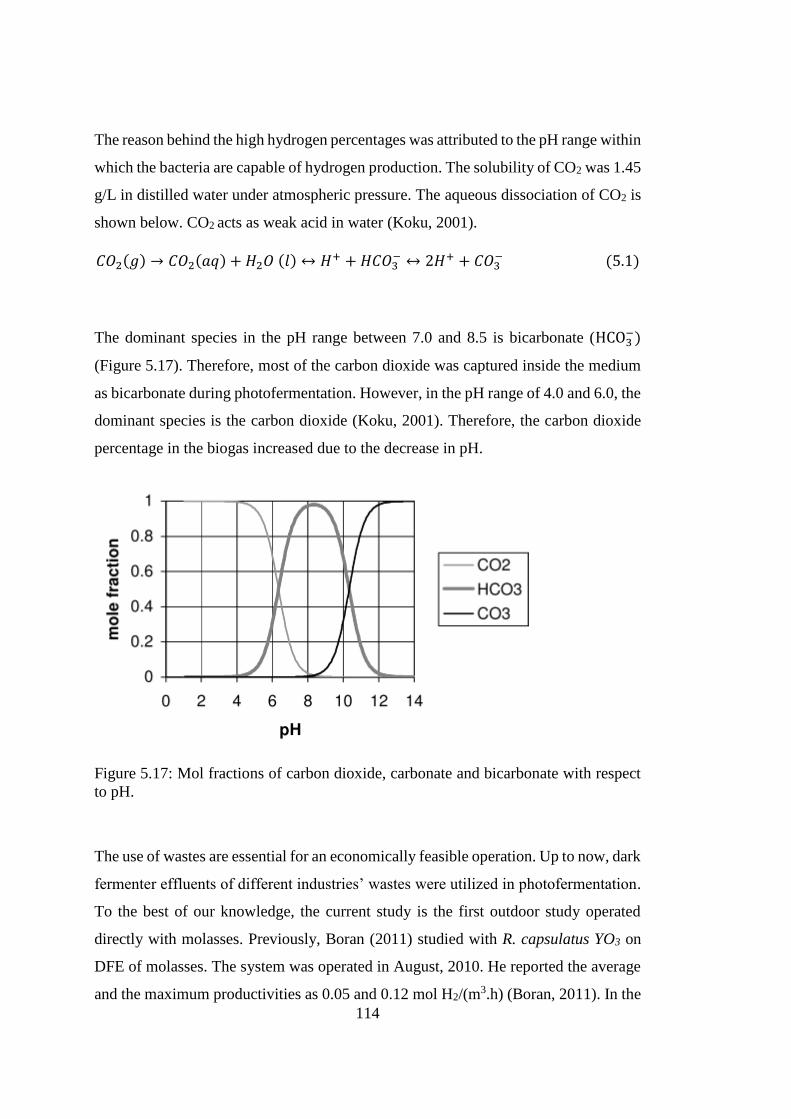
114

The reason behind the high hydrogen percentages was attributed to the pH range within

which the bacteria are capable of hydrogen production. The solubility of CO2 was 1.45

g/L in distilled water under atmospheric pressure. The aqueous dissociation of CO2 is

shown below. CO2 acts as weak acid in water (Koku, 2001).

𝐶𝑂2(𝑔) → 𝐶𝑂2(𝑎𝑞) + 𝐻2𝑂 (𝑙) ↔ 𝐻+ + 𝐻𝐶𝑂3− ↔ 2𝐻+ + 𝐶𝑂3

− (5.1)

The dominant species in the pH range between 7.0 and 8.5 is bicarbonate (HCO3−)

(Figure 5.17). Therefore, most of the carbon dioxide was captured inside the medium

as bicarbonate during photofermentation. However, in the pH range of 4.0 and 6.0, the

dominant species is the carbon dioxide (Koku, 2001). Therefore, the carbon dioxide

percentage in the biogas increased due to the decrease in pH.

Figure 5.17: Mol fractions of carbon dioxide, carbonate and bicarbonate with respect

to pH.

The use of wastes are essential for an economically feasible operation. Up to now, dark

fermenter effluents of different industries’ wastes were utilized in photofermentation.

To the best of our knowledge, the current study is the first outdoor study operated

directly with molasses. Previously, Boran (2011) studied with R. capsulatus YO3 on

DFE of molasses. The system was operated in August, 2010. He reported the average

and the maximum productivities as 0.05 and 0.12 mol H2/(m3.h) (Boran, 2011). In the

115

current study, the productivity increased significantly, reporting the average and the

maximum productivities as 0.16 and 0.31 mol H2/(m3.h). Therefore, in the current

study the productivity was increased around 3 fold.

5.3 Overall Evaluation of the Stacked U-tube Reactor and the Comparison of

Productivities with Other Outdoor Studies

The bottleneck of photofermentation is its high capital and operating costs. The main

capital cost item of photofermentation is the rent for large ground area (Urbaniec &

Grabarczyk, 2014). With this reactor, the ground area to volume ratio (2.41 m-1) was

reduced compared to tubular or nearly tubular PBRs. This ratio can be further reduced

with the addition of more tubes to the manifolds. In a recent study, the reason behind

the high operational costs for tubular PBRs was found as the LDPE tubes which needs

to be changed every year (Urbaniec & Grabarczyk, 2014). Therefore, the material

selection is quite important for PBRs. Glass having less permeability of hydrogen and

air than LDPE tubes is a good choice for PBR. Moreover, glass is more durable in

outdoor conditions, and its life time is much more (~20 years). With stacked U-tube

reactor, the capital and operational cost of PBR is reduced.

In this study, molasses was utilized as the feedstock for photofermentation for the first

time in literature. From the results of RUN 092014, a proper feeding strategy was

proposed for outdoor operations when molasses was used as the feedstock. With the

light of the information obtained for this run, the stacked U-tube PBR was operated

successfully with R. capsulatus YO3 on molasses between July 12 and July 24, 2015.

Another reactor working with R. capsulatus YO3 on acetate was also run in parallel.

The experimental results of these runs were summarized in Table 5.4.

Hydrogen productivity enhanced 3 folds when compared with the outdoor experiment

performed with R. capsulatus YO3 on DFE of molasses (Boran, 2011). Moreover, the

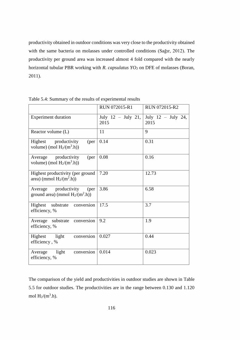
116

productivity obtained in outdoor conditions was very close to the productivity obtained

with the same bacteria on molasses under controlled conditions (Sağır, 2012). The

productivity per ground area was increased almost 4 fold compared with the nearly

horizontal tubular PBR working with R. capsulatus YO3 on DFE of molasses (Boran,

2011).

Table 5.4: Summary of the results of experimental results

RUN 072015-R1 RUN 072015-R2

Experiment duration July 12 – July 21,

2015

July 12 – July 24,

2015

Reactor volume (L) 11 9

Highest productivity (per

volume) (mol H2/(m3.h))

0.14 0.31

Average productivity (per

volume) (mol H2/(m3.h))

0.08 0.16

Highest productivity (per ground

area) (mmol H2/(m2.h))

7.20 12.73

Average productivity (per

ground area) (mmol H2/(m2.h))

3.86 6.58

Highest substrate conversion

efficiency, %

17.5 3.7

Average substrate conversion

efficiency, %

9.2 1.9

Highest light conversion

efficiency , %

0.027 0.44

Average light conversion

efficiency, %

0.014 0.023

The comparison of the yield and productivities in outdoor studies are shown in Table

5.5 for outdoor studies. The productivities are in the range between 0.130 and 1.120

mol H2/(m3.h).

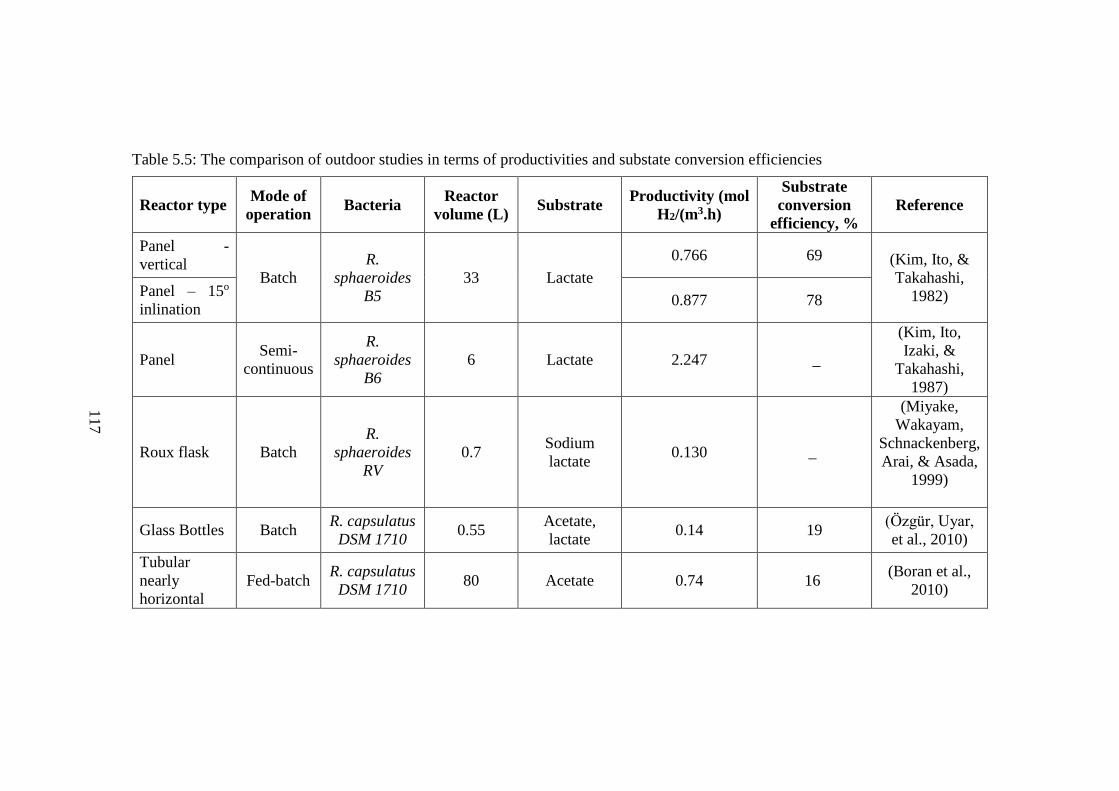
117

Table 5.5: The comparison of outdoor studies in terms of productivities and substate conversion efficiencies

Reactor type Mode of

operation Bacteria

Reactor

volume (L) Substrate

Productivity (mol

H2/(m3.h)

Substrate

conversion

efficiency, %

Reference

Panel -

vertical Batch

R.

sphaeroides

B5

33 Lactate

0.766 69 (Kim, Ito, &

Takahashi,

1982) Panel – 15o

inlination 0.877 78

Panel Semi-

continuous

R.

sphaeroides

B6

6 Lactate 2.247 _

(Kim, Ito,

Izaki, &

Takahashi,

1987)

Roux flask Batch

R.

sphaeroides

RV

0.7 Sodium

lactate 0.130 _

(Miyake,

Wakayam,

Schnackenberg,

Arai, & Asada,

1999)

Glass Bottles Batch R. capsulatus

DSM 1710 0.55

Acetate,

lactate 0.14 19

(Özgür, Uyar,

et al., 2010)

Tubular

nearly

horizontal

Fed-batch R. capsulatus

DSM 1710 80 Acetate 0.74 16

(Boran et al.,

2010)

117

118

Table 5.5.continued

Reactor type Mode of

operation Bacteria

Reactor

volume

(L)

Substrate Productivity (mol

H2/(m3.h)

Substrate

conversion

efficiency, %

Reference

Panel Batch

R.

sphaeroides

O.U.001

(DSM 5864)

6.5

Malate 0.225 - 0.449 10 - 77 (Eroǧlu,

Tabanoǧlu,

Gündüz,

Eroǧlu, &

Yücel, 2008)

Acetate 0.36 30

Lactate /

Olive mill

wastewater

0.090 / 0.135 13

Outdoor Fed-batch R. capsulatus

JP91 4

DFE of thick

juice 1.12 __

(Özkan et al.,

2012)

Panel Fed-batch R. capsulatus

DSM 155 25L x 4

Acetate,

lactate 0.94 __

(Jacub

Gebicki,

Modigell,

Schumacher,

Van Der

Burg, &

Roebroeck,

2009)

118

119

Table 5.5.continued

Outdoor Fed-batch

R.

capsulatus

YO3 (hup-)

90 Acetate 0.4 12

(Boran et

al., 2012b)

Outdoor Fed-batch

R.

capsulatus

DSM 1710

90 DFE of

thick juice 0.27 12

Reactor

type

Mode of

operation Bacteria

Reactor

volume

(L)

Substrate Productivity

(mol H2/(m3.h)

Substrate

conversion

efficiency,

%

Reference

Tubular,

nearly

horizontal

Fed -

batch

R.

capsulatus

hup -

(YO3)

90

Acetic acid

- DFE of

thick juice

0.4 9 (Boran et

al., 2012a)

Tubular,

nearly

horizantal

Fed -

batch

R.

capsulatus

hup -

(YO3)

90

Acetic acid

- DFE of

thick juice

0.27 10 (Boran et

al., 2012b)

Acetic acid 0.74 15

Outdoor Fed-batch

Rp.

palustris

420L

50 malate 0.48 10 (Adessi et

al., 2012)

119

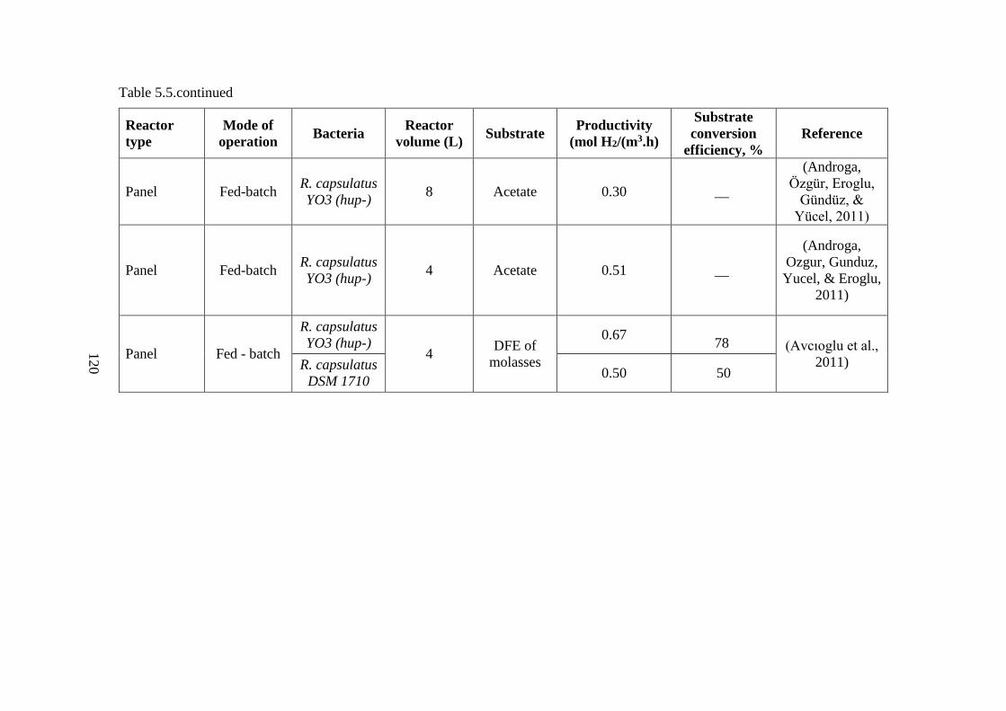
120

Table 5.5.continued

Reactor

type

Mode of

operation Bacteria

Reactor

volume (L) Substrate

Productivity

(mol H2/(m3.h)

Substrate

conversion

efficiency, %

Reference


YO3 (hup-) 8 Acetate 0.30 __

(Androga,

Özgür, Eroglu,

Gündüz, &

Yücel, 2011)


YO3 (hup-) 4 Acetate 0.51 __

(Androga,

Ozgur, Gunduz,

Yucel, & Eroglu,

2011)

Panel Fed - batch

R. capsulatus

YO3 (hup-) 4

DFE of

molasses

0.67

78 (Avcıoglu et al.,

2011) R. capsulatus

DSM 1710 0.50 50

120

121

CHAPTER 6

CONCLUSIONS AND RECOMMENDATIONS

A new stacked-tubular design was proposed in this study with the goal of addressing

problems with scale up of PBRs for hydrogen production. A hydrodynamic model for

this design was developed utilizing COMSOL Multiphysics 4.1. The effects of tube

pitch, tube length and volumetric flow rate on the flow distribution were investigated

in the model. The most uniform flow distribution with a non-uniformity parameter of

1.5% was obtained for a tube pitch of 10.5 cm, a tube length of 3.8 m and a volumetric

flow rate of 25 L/h. Then, the stacked U-tube PBR was constructed. The dimensions

of the PBR (10.5 cm tube pitch and 4 m tube length) were based on the model results.

In view of its lower long-term material costs and low permeability to hydrogen and

air, glass was chosen as the reactor material. The illuminated surface area to ground

area of the reactor was found as 5:1, a high value for tubular-type reactors. Moreover,

the volume to ground area ratio (2.44 m-1) is very high compared to other tubular

reactors. The PBR proposed in this thesis is a much more suitable one for

photofermentative hydrogen production compared to the panel or slightly inclined

horizontal tubular reactors.

The tube diameter was selected based on the photon counts and absorbencies of

molasses at different depths. The tube diameter was selected as 3 cm for

photofermentative hydrogen production purposes under outdoor conditions.

122

Centrifugal and peristaltic pump types were compared in terms of bacterial growth in

the greenhouse utilizing U-tubes. Although there was not a significant difference in

bacterial growth between the pumps, the peristaltic pump was preferred for the pilot-

scale experiments, since it is easier to control the flow rate with a peristaltic pump.

A proper feeding strategy is essential to test the stacked U-tube PBR. An experiment

(RUN 092014) was carried out in September 2014 using molasses as the carbon source

and Rhodobacter capsulatus YO3 (Hup-) as the microorganism. The PBR was tested

in outdoor conditions with R. capsulatus YO3 on molasses in September, 2014.

Evaluation of the sucrose consumption rate and organic acid production rate gave an

insight about the feeding strategy for future applications. From the results of this run,

it has been concluded that the sucrose content in the reactor should be maintained

above 5 mM, and acetic acid and lactic acid content should be kept below 40 mM.

These values lead to establish the feeding strategy for the succeeding experiments.

Two experiments were run successfully in parallel in July 2015. RUN 072015-R1 was

run with Rhodobacter capsulatus YO3 (hup-) on acetate. The feeding strategy was to

keep the acetic acid concentration 40 mM in the reactor. The maximum substrate

conversion efficiency was calculated on the 3rd day of the experiment as 17.5%.

Average substrate conversion efficiency was found as 9.2%. The highest light

conversion efficiency was found on the 2nd day as 0.021%. The highest and the average

productivity was found as 0.144 and 0.077 mol H2/(m3.h), respectively. The highest

productivity was observed on the 2nd day before continuous feeding started. Another

reactor containing Rhodobacter capsulatus YO3 (hup-) was operated with molasses

(RUN 072015-R2). This is the first time that molasses was utilized directly for

photofermentation in outdoor conditions. The feeding strategy was based on the

previous experimental results. The maximum substrate conversion efficiency was

found as 3.65% on the 10th day of the experiment. The average substrate conversion

efficiency was found as 1.89%. The highest light conversion efficiency of this reactor

was 0.044 % on the 10th day. Hydrogen production observed mainly after continuous

123

feeding started. The highest and the average productivity was found as 0.311 and 0.161

respectively. It has been concluded that hydrogen productivity is higher with molasses

used as substrate compared to acetate. Therefore single stage photofermentation with

molasses is more advantageous compared to two-stage biological hydrogen

production; dark fermentation followed by photofermentation.

Some recommendations for future studies are listed below.

A kinetic analysis is necessary to figure out the sucrose consumption rate and

organic acid production rates and to suggest a better feeding strategy.

Productivity was decreased due to low pH values in the PBR operating with

molasses. Therefore, a pH control system should be adopted for the reactor.

All of the sucrose supplied by molasses was consumed every day in RUN

072015-R2. Therefore, sucrose content can be increased up to 10 mM or more

for higher productivities. However, without a proper pH controller, increasing

the sucrose concentration in molasses will result in a decrease in pH.

Most of the biogas is produced in the tubes. In order to collect the gas

accumulated in the tubes, the flow rate of the reactor could be increased for a

while. Since the bacteria cannot withstand the stress created by turbulent flow

regime, the maximum flow rate should be adjusted such that Reynolds number

in the tubes will be at most 2100. The duration should be equal to or more than

the residence time to collect all the gas properly.

If such as reactor is to be operated in much larger scale, the number of

connections should be reduced to prevent the risk of leakage. However, while

welding glass, there can be some small errors in dimensions if the glass pieces

is not cast in mold. If all glass pieces is to be welded, the system loses its

flexibility, and it gets harder to connect the glass pieces to the stand. Moreover,

glass breaks easily during construction. It is easier to change the pieces, if they

are not all welded. Considering these issues, the optimum number of

connections should be determined for larger volume systems.

124

More tubes can be added to the reactor to increase the reactor volume. By this

way, the illuminated area to ground area ratio will get higher. However, the

flow model of such systems should also be investigated to obtain the most

uniform flow distribution.

125

REFERENCES

Abdul, P. M., Md. Jahim, J., Harun, S., Markom, M., Hassan, O., Mohammad, A. W.,

& Asis, A. J. (2013). Biohydrogen production from pentose-rich oil palm empty

fruit bunch molasses: A first trial. International Journal of Hydrogen Energy,

XXX, 1–7.

Ablanque, N., Oliet, C., Rigola, J., Pérez-Segarra, C. D., & Oliva, A. (2010). Two-

phase flow distribution in multiple parallel tubes. International Journal of

Thermal Sciences, 49, 909–921.

Abo-Hashesh, M., Ghosh, D., Tourigny, A., Taous, A., & Hallenbeck, P. C. (2011).

Single stage photofermentative hydrogen production from glucose: An attractive

alternative to two stage photofermentation or co-culture approaches.

International Journal of Hydrogen Energy, 36(21), 13889–13895.

Acrivos, A., Babcock, B. D., & Pigford, R. L. (1959). Flow distributions in manifolds.

Chemical Engineering Science, 10(1-2), 112–124.

Adessi, A., Torzillo, G., Baccetti, E., & De Philippis, R. (2012). Sustained outdoor H2

production with Rhodopseudomonas palustris cultures in a 50 L tubular

photobioreactor. International Journal of Hydrogen Energy, 37(10), 8840–8849.

Afsar, N., Özgür, E., Gürgan, M., Akköse, S., Yücel, M., Gündüz, U., & Eroglu, I.

(2011). Hydrogen productivity of photosynthetic bacteria on dark fermenter

effluent of potato steam peels hydrolysate. International Journal of Hydrogen

Energy, 36(1), 432–438.

Ahn, H., Lee, S., & Shin, S. (1998). Flow Distribution in manifolds for low Reynolds

number flow. KSME International Journal, 12(1), 87–95.

Akkerman, I., Janssen, M., Rocha, J., & H, W. R. (2002). Photobiological hydorgen

production: photochemical efficiency and bioreactor design. International

Journal of Hydrogen Energy, 27(11-12), 1195–1208.

Androga, D. D. (2009). Biological hydrogen production on acetate in continuous

panel photobioreactors using Rhodobacter capsulatus. M. Sc Thesis submitted

to Chemical Engineering Department of Middle East Technical University.

126

Androga, D. D. (2014). Modelling and simulation of photobioreactors for biological

hydrogen production. PhD. Thesis submitted to Department of Biotechnology of

Middle East Technical University.

Androga, D. D., Ozgur, E., Gunduz, U., Yucel, M., & Eroglu, I. (2011). Factors

affecting the longterm stability of biomass and hydrogen productivity in outdoor

photofermentation. International Journal of Hydrogen Energy, 36(17), 11369–

11378.

Androga, D. D., Özgür, E., & Eroglu, I. (2012). Amelioration of photofermentative

hydrogen production from molasses dark fermenter effluent by zeolite-based

removal of ammonium ion. International Journal of Hydrogen Energy, 37(21),

16421–16429.

Androga, D. D., Özgür, E., Eroglu, I., Gündüz, U., & Yücel, M. (2011). Significance

of carbon to nitrogen ratio on the long-term stability of continuous

photofermentative hydrogen production. International Journal of Hydrogen

Energy, 36(24), 15583–15594.

Androga, D. D., Özgür, E., Eroglu, I., Gündüz, U., & Yücel, M. (2012).

Photofermentative Hydrogen Production in Outdoor Conditions. In D. Minic

(Ed.), Hydrogen Energy - Challenges and Perspectives. InTech.

Ángel, M.-D. J., Manuel, O.-R. J., Omar, J.-S., Antonio, Z.-A. M., & Armando, E.-O.

(2013). Analysis of Flow and Heat Transfer in a Flat Solar Collector with

Rectangular and Cylindrical Geometry Using CFD. Ingeniería, Investigación Y

Tecnología, 14(4), 553–561.

Argun, H., & Kargi, F. (2010a). Effects of light source, intensity and lighting regime

on bio-hydrogen production from ground wheat starch by combined dark and

photo-fermentations. International Journal of Hydrogen Energy, 35(4), 1604–

1612.

Argun, H., & Kargi, F. (2010b). Photo-fermentative hydrogen gas production from

dark fermentation effluent of ground wheat solution: Effects of light source and

light intensity. International Journal of Hydrogen Energy, 35(4), 1595–1603.

Argun, H., & Kargi, F. (2011). Bio-hydrogen production by different operational

modes of dark and photo-fermentation: An overview. International Journal of

Hydrogen Energy, 36(13), 7443–7459.

Argun, H., Kargi, F., & Kapdan, I. K. (2009). Effects of the substrate and cell

concentration on bio-hydrogen production from ground wheat by combined dark

and photo-fermentation. International Journal of Hydrogen Energy, 34(15),

6181–6188.

127

Asada, Y., Tokumoto, M., Aihara, Y., Oku, M., Ishimi, K., Wakayama, T., … Kohno,

H. (2006). Hydrogen production by co-cultures of Lactobacillus and a

photosynthetic bacterium, Rhodobacter sphaeroides RV. International Journal of


Avcioglu, S. G. (2010). Scale up of panel photobioreactors for hydrogen production

by PNS bacteria. M.Sc. Thesis submitted to Chemical Engineering Department

of Middle East Technical University

Avcıoglu, S. G., Özgur, E., Eroglu, I., Yücel, M., & Gündüz, U. (2011). Biohydrogen

production in an outdoor panel photobioreactor on dark fermentation effluent of

molasses. International Journal of Hydrogen Energy, 36(17), 11360–11368.

Ball, M., & Wietschel, M. (2009). The future of hydrogen - opportunities and

challenges. International Journal of Hydrogen Energy, 34(2), 615–627.

Barbosa, M. J., Rocha, J. M. S., Tramper, J., & Wijffels, R. H. (2001). Acetate as a

carbon source for hydrogen production by photosynthetic bacteria. Journal of

Biotechnology, 85(1), 25–33.

Basak, N., & Das, D. (2009). Photofermentative hydrogen production using purple

non-sulfur bacteria Rhodobacter sphaeroides O.U.001 in an annular

photobioreactor: A case study. Biomass and Bioenergy, 33(6-7), 911–919.

Benemann, J. R., Berenson, J. a, Kaplan, N. O., & Kamen, M. D. (1973). Hydrogen

evolution by a chloroplast-ferredoxin-hydrogenase system. Proceedings of the

National Academy of Sciences of the United States of America, 70(8), 2317–2320.

Biebl, H., & Pfennig, N. (1981). Isolation of members of the family Chloroflexaceae.

In H. G. Starr, Mortimer P.; Stolp, Heinz; Trüper, Hans G.; Balows, Albert;

Schlegel (Ed.), The Prokaryotes (pp. 267–273). Springer-Verlag.

Boran, E. (2011). Process development for continuous photofermentative hydrogen

production. Middle East Technical University. M.Sc. Thesis submitted to

Chemical Engineering Department of Middle East Technical University

Boran, E., Özgür, E., Van Der Burg, J., Yücel, M., Gündüz, U., & Eroglu, I. (2010).

Biological hydrogen production by Rhodobacter capsulatus in solar tubular photo

bioreactor. Journal of Cleaner Production, 18(SUPPL. 1), S29–S35.

Boran, E., Özgür, E., Yücel, M., Gündüz, U., & Eroglu, I. (2012a). Biohydrogen

production by Rhodobacter capsulatus Hup− mutant in pilot solar tubular

photobioreactor. International Journal of Hydrogen Energy, 37(21), 16437–

16445.

128

Boran, E., Özgür, E., Yücel, M., Gündüz, U., & Eroglu, I. (2012b). Biohydrogen

production by Rhodobacter capsulatus in solar tubular photobioreactor on thick

juice dark fermenter effluent. Journal of Cleaner Production, 31, 150–157.

Brentner, L. B., Peccia, J., & Zimmerman, J. B. (2010). Challenges in developing

biohydrogen as a sustainable energy source: implications for a research agenda.

Environmental Science & Technology, 44(7), 2243–2254.

Chen, C., Lee, C., & Chang, J. (2006). Feasibility study on bioreactor strategies for

enhanced photohydrogen production from Rhodopseudomonas palustris WP3-5

using optical-fiber-assisted illumination systems. International Journal of


Chen, C. Y., & Chang, J. S. (2006). Enhancing phototropic hydrogen production by

solid-carrier assisted fermentation and internal optical-fiber illumination. Process

Biochemistry, 41(9), 2041–2049.

Chen, C. Y., Lee, C. M., & Chang, J. S. (2006). Hydrogen production by indigenous

photosynthetic bacterium Rhodopseudomonas palustris WP3-5 using optical

fiber-illuminating photobioreactors. Biochemical Engineering Journal, 32(1),

33–42.

Chen, C. Y., Yang, M. H., Yeh, K. L., Liu, C. H., & Chang, J. S. (2008). Biohydrogen

production using sequential two-stage dark and photo fermentation processes.


Chen, C. Y., Yeh, K. L., Lo, Y. C., Wang, H. M., & Chang, J. S. (2010). Engineering

strategies for the enhanced photo-H2 production using effluents of dark

fermentation processes as substrate. International Journal of Hydrogen Energy,

35(24), 13356–13364.

Chen, C.-H., Jung, S.-P., & Yen, S.-C. (2007). Flow distribution in the manifold of

PEM fuel cell stack. Journal of Power Sources, 173, 249–263.

Cheng, J., Su, H., Zhou, J., Song, W., & Cen, K. (2011). Hydrogen production by

mixed bacteria through dark and photo fermentation. International Journal of


Comsol. (2012a). COMSOL Multiphysics Reference Guide, 569–613. Retrieved from

http://www.comsol.com/

Comsol. (2012b). Comsol Multiphysics User’s Guid. Retrieved from

http://www.comsol.com/

Das, D., & Veziroglu, T. N. (2001). Hydrogen production by biological processes: a

survey of literature. International Journal of Hydrogen Energy, 26(1), 13–28.

129

Dasgupta, C. N., Jose Gilbert, J., Lindblad, P., Heidorn, T., Borgvang, S. a., Skjanes,

K., & Das, D. (2010). Recent trends on the development of photobiological

processes and photobioreactors for the improvement of hydrogen production.


Datar, R., Huang, J., Maness, P. C., Mohagheghi, A., Czernik, S., & Chornet, E.

(2007). Hydrogen production from the fermentation of corn stover biomass

pretreated with a steam-explosion process. International Journal of Hydrogen

Energy, 32(8), 932–939.

Ding, J., Liu, B. F., Ren, N. Q., Xing, D. F., Guo, W. Q., Xu, J. F., & Xie, G. J. (2009).

Hydrogen production from glucose by co-culture of Clostridium Butyricum and

immobilized Rhodopseudomonas faecalis RLD-53. International Journal of


Eroglu, E., Gunduz, U., Yucel, M., & Eroglu, I. (2011). Effect of iron and molybdenum

addition on photofermentative hydrogen production from olive mill wastewater.


Eroglu, I., Özgür, E., Eroglu, E., Yücel, M., & Gündüz, U. (2014). Applications of

photofermentative hydrogen production. In D. Zannoni & R. De Philippis (Eds.),

Microbial Bioenergy: Hydrogen Production (pp. 237–267). Springer.

Eroǧlu, I., Tabanoǧlu, A., Gündüz, U., Eroǧlu, E., & Yücel, M. (2008). Hydrogen

production by Rhodobacter sphaeroides O.U.001 in a flat plate solar bioreactor.


Fan, J., Shah, L. J., & Furbo, S. (2007). Flow distribution in a solar collector panel

with horizontally inclined absorber strips. Solar Energy, 81, 1501–1511.

Fang, H. H. P., Zhu, H., & Zhang, T. (2006). Phototrophic hydrogen production from

glucose by pure and co-cultures of Clostridium butyricum and Rhodobacter

sphaeroides. International Journal of Hydrogen Energy, 31(15), 2223–2230.

Fernandez-Sevilla, J. M., Acien-Fernandez, F. G., & Molina-Grima, E. (2014).

Photobioreactors design for hydrogen production. In D. Zannoni & R. De

Philippis (Eds.), Microbial Bioenergy: Hydrogen Production. Springer.

Flickinger, M. C. (2013). Upstream Industrial Biotechnology, 2 Volume Set. John

Wiley & Sons.

Gebicki, J., Modigell, M., Schumacher, M., Van Der Burg, J., & Roebroeck, E. (2009).

Development of photobioreactors for anoxygenic production of hydrogen by

purple bacteria. Chemical Engineering Transactions, 18, 363–366.

Gebicki, J., Modigell, M., Schumacher, M., Van Der Burg, J., & Roebroeck, E. (2010).

Comparison of two reactor concepts for anoxygenic H2 production by

130

Rhodobacter capsulatus. Journal of Cleaner Production, 18(SUPPL. 1), S36–

S42.

Ghosh, D., Sobro, I. F., & Hallenbeck, P. C. (2012). Optimization of the hydrogen

yield from single-stage photofermentation of glucose by Rhodobacter capsulatus

JP91 using response surface methodology. Bioresource Technology, 123, 199–

206.

Guo, C. L., Zhu, X., Liao, Q., Wang, Y. Z., Chen, R., & Lee, D. J. (2011).

Enhancement of photo-hydrogen production in a biofilm photobioreactor using

optical fiber with additional rough surface. Bioresource Technology, 102(18),

8507–8513.

Guo, W. Q., Ren, N. Q., Wang, X. J., Xiang, W. S., Meng, Z. H., Ding, J., … Zhang,

L. S. (2008). Biohydrogen production from ethanol-type fermentation of

molasses in an expanded granular sludge bed (EGSB) reactor. International

Journal of Hydrogen Energy, 33(19), 4981–4988.

Hallebeck, P. C. (2014). Bioenergy from Microorganisms: An Overview. In D.

Zannoni & R. De Philips (Eds.), Microbial Bioenergy: Hydrogen Production (pp.

3–21). Springer.

Hallenbeck, P. C., & Benemann, J. R. (2002). Biological hydrogen production;

Fundamentals and limiting processes. International Journal of Hydrogen Energy,

27(11-12), 1185–1193.

Hallenbeck, P. C., & Ghosh, D. (2009). Advances in fermentative biohydrogen

production: the way forward? Trends in Biotechnology, 27(5), 287–297.

Hawkes, F. R., Dinsdale, R., Hawkes, D. L., & Hussy, I. (2002). Sustainable

fermentative hydrogen production: Challenges for process optimisation.

International Journal of Hydrogen Energy, 27(11-12), 1339–1347.

International Energy Agency. (2015). Energy and climate change. Paris.

Jeong, T. Y., Cha, G. C., Yoo, I. K., & Kim, D. J. (2007). Hydrogen production from

waste activated sludge by using separation membrane acid fermentation reactor

and photosynthetic reactor. International Journal of Hydrogen Energy, 32(5),

525–530.

Kataoka, N., Miya, A., & Kiriyama, K. (1997). Studies on hydrogen production by

continuous culture system of hydrogen-producing anaerobic bacteria. Water

Science and Technology, 36(6-7), 41–47.

Keskin, T., & Hallenbeck, P. C. (2012). Hydrogen production from sugar industry

wastes using single-stage photofermentation. Bioresource Technology, 112, 131–

136.

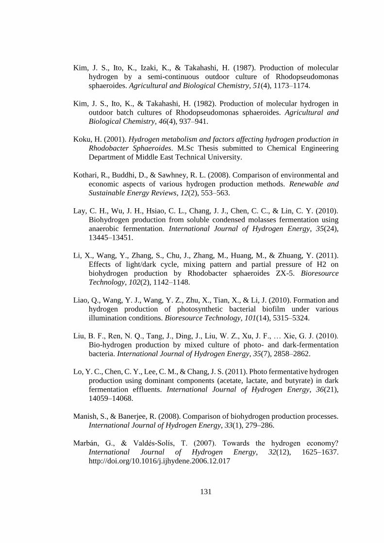
131

Kim, J. S., Ito, K., Izaki, K., & Takahashi, H. (1987). Production of molecular

hydrogen by a semi-continuous outdoor culture of Rhodopseudomonas

sphaeroides. Agricultural and Biological Chemistry, 51(4), 1173–1174.

Kim, J. S., Ito, K., & Takahashi, H. (1982). Production of molecular hydrogen in

outdoor batch cultures of Rhodopseudomonas sphaeroides. Agricultural and

Biological Chemistry, 46(4), 937–941.

Koku, H. (2001). Hydrogen metabolism and factors affecting hydrogen production in

Rhodobacter Sphaeroides. M.Sc Thesis submitted to Chemical Engineering

Department of Middle East Technical University.

Kothari, R., Buddhi, D., & Sawhney, R. L. (2008). Comparison of environmental and

economic aspects of various hydrogen production methods. Renewable and

Sustainable Energy Reviews, 12(2), 553–563.

Lay, C. H., Wu, J. H., Hsiao, C. L., Chang, J. J., Chen, C. C., & Lin, C. Y. (2010).

Biohydrogen production from soluble condensed molasses fermentation using

anaerobic fermentation. International Journal of Hydrogen Energy, 35(24),

13445–13451.

Li, X., Wang, Y., Zhang, S., Chu, J., Zhang, M., Huang, M., & Zhuang, Y. (2011).

Effects of light/dark cycle, mixing pattern and partial pressure of H2 on

biohydrogen production by Rhodobacter sphaeroides ZX-5. Bioresource

Technology, 102(2), 1142–1148.

Liao, Q., Wang, Y. J., Wang, Y. Z., Zhu, X., Tian, X., & Li, J. (2010). Formation and

hydrogen production of photosynthetic bacterial biofilm under various

illumination conditions. Bioresource Technology, 101(14), 5315–5324.

Liu, B. F., Ren, N. Q., Tang, J., Ding, J., Liu, W. Z., Xu, J. F., … Xie, G. J. (2010).

Bio-hydrogen production by mixed culture of photo- and dark-fermentation

bacteria. International Journal of Hydrogen Energy, 35(7), 2858–2862.

Lo, Y. C., Chen, C. Y., Lee, C. M., & Chang, J. S. (2011). Photo fermentative hydrogen

production using dominant components (acetate, lactate, and butyrate) in dark

fermentation effluents. International Journal of Hydrogen Energy, 36(21),

14059–14068.

Manish, S., & Banerjee, R. (2008). Comparison of biohydrogen production processes.


Marbán, G., & Valdés-Solís, T. (2007). Towards the hydrogen economy?


http://doi.org/10.1016/j.ijhydene.2006.12.017

132

Miyake, J., Wakayama, T., Schnackenberg, J., Arai, T., & Asada, Y. (1999).

Simulation of the daily sunlight illumination pattern for bacterial photo-hydrogen

production. Journal of Bioscience and Bioengineering, 88(6), 659–663.

http://doi.org/10.1016/S1389-1723(00)87096-6

Nakada, E., Asada, Y., Arai, T., & Miyake, J. (1995). Light penetration into cell

suspensions of photosynthetic bacteria and relation to hydrogen production.

Journal of Fermentation and Bioengineering, 80(1), 53–57.

http://doi.org/10.1016/0922-338X(95)98176-L

Nath, K., & Das, D. (2004). Biohydrogen production as a potential energy resource –

Present state-of-art. Journal of Scientific & Industrial Research, 63(September),

729–738.

Nath, K., Muthukumar, M., Kumar, A., & Das, D. (2008). Kinetics of two-stage

fermentation process for the production of hydrogen. International Journal of



Ntaikou, I., Gavala, H. N., Kornaros, M., & Lyberatos, G. (2008). Hydrogen

production from sugars and sweet sorghum biomass using Ruminococcus albus.



Ogden, J. M. (1999). Prospects for Building a Hydrogen Energy Infrastructure. Annual

Review of Energy and the Environment, 24(1), 227–279.

http://doi.org/10.1146/annurev.energy.24.1.227

Ozmihci, S., & Kargi, F. (2010). Bio-hydrogen production by photo-fermentation of

dark fermentation effluent with intermittent feeding and effluent removal.



Özgür, E., Afsar, N., De Vrije, T., Yücel, M., Gündüz, U., Claassen, P. a M., & Eroglu,

I. (2010). Potential use of thermophilic dark fermentation effluents in

photofermentative hydrogen production by Rhodobacter capsulatus. Journal of

Cleaner Production, 18(SUPPL. 1), S23–S28.

http://doi.org/10.1016/j.jclepro.2010.02.020

Özgür, E., Mars, A. E., Peksel, B., Louwerse, A., Yücel, M., Gündüz, U., … Eroğlu,

I. (2010). Biohydrogen production from beet molasses by sequential dark and

photofermentation. International Journal of Hydrogen Energy, 35(2), 511–517.


Özgür, E., & Peksel, B. (2013). Biohydrogen production from barley straw hydrolysate

through sequential dark and photofermentation. Journal of Cleaner Production,

52, 14–20. http://doi.org/10.1016/j.jclepro.2013.02.035

133

Özgür, E., Uyar, B., Öztürk, Y., Yücel, M., Gündüz, U., & Eroǧlu, I. (2010).

Biohydrogen production by Rhodobacter capsulatus on acetate at fluctuating

temperatures. Resources, Conservation and Recycling, 54(5), 310–314.

http://doi.org/10.1016/j.resconrec.2009.06.002

Özkan, E., Uyar, B., Özgür, E., Yücel, M., Eroglu, I., & Gündüz, U. (2012).

Photofermentative hydrogen production using dark fermentation effluent of sugar

beet thick juice in outdoor conditions. International Journal of Hydrogen Energy,

37(2), 2044–2049. http://doi.org/10.1016/j.ijhydene.2011.06.035

Öztürk, Y. (2005). Characterization of the genetically modified cytochrome systems

and their application to biohydrogen production in Rhodobacter capsulatus. PhD

thesis submitted to Department of Biotechnology of Middle East Technical

University.

Öztürk, Y., Yücel, M., Daldal, F., Mandaci, S., Gündüz, U., Türker, L., & Eroǧlu, I.

(2006). Hydrogen production by using Rhodobacter capsulatus mutants with

genetically modified electron transfer chains. International Journal of Hydrogen

Energy, 31(11), 1545–1552. http://doi.org/10.1016/j.ijhydene.2006.06.042

Panwar, N. L., Kaushik, S. C., & Kothari, S. (2011). Role of renewable energy sources

in environmental protection: A review. Renewable and Sustainable Energy

Reviews, 15(3), 1513–1524. http://doi.org/10.1016/j.rser.2010.11.037

Perera, K. R. J., Ketheesan, B., Gadhamshetty, V., & Nirmalakhandan, N. (2010).

Fermentative biohydrogen production: Evaluation of net energy gain.



Pilavachi, P. a., Chatzipanagi, A. I., & Spyropoulou, A. I. (2009). Evaluation of

hydrogen production methods using the Analytic Hierarchy Process.



Redwood, M., & Macaskie, L. (2006). A two-stage, two-organism process for

biohydrogen from glucose. International Journal of Hydrogen Energy, 31(11),

1514–1521. http://doi.org/10.1016/j.ijhydene.2006.06.018

Ren, N., Li, J., Li, B., Wang, Y., & Liu, S. (2006). Biohydrogen production from

molasses by anaerobic fermentation with a pilot-scale bioreactor system.



Ren, N. Q., Liu, B. F., Zheng, G. X., Xing, D. F., Zhao, X., Guo, W. Q., & Ding, J.

(2009). Strategy for enhancing photo-hydrogen production yield by repeated fed-

batch cultures. International Journal of Hydrogen Energy, 34(18), 7579–7584.


134

Sağır, E. (2012). Photobiological hydrogen production from sugar beet molasses.

M.Sc. Thesis submitted to the Department of Biochemistry of Middle East

Technical University.

Sasikala, K., Ramama, C. V., & Raghuveer Rao, P. (1991). Environmental regulation

for optimal biomass yield and photoproduction of hydrogen by Rhodobacter

sphaeroides O.U.001. Biotechnology, 16(9), 597–601.

Sievert, V. (2003). Two-phase flow distribution in compact heat exchanger manifolds.

Norvegian University of Science and Technology. Retrieved from

http://www.mendeley.com/research/twophase-flow-distribution-heat-exchanger-

manifolds/

Spruit, C. J. P. (1958). Simultaneous photoproduction of hydrogen and oxygen by

Chlorella. Mededelingen van de Landbouwhogeschool Te Wageningen, 58, 1–17.

Retrieved from http://www.amazon.co.uk/Simultaneous-photoproduction-

Mededelingen-Landbouwhogeschool-Wageningen/dp/B0007J6PKS

Su, H., Cheng, J., Zhou, J., Song, W., & Cen, K. (2009a). Combination of dark- and

photo-fermentation to enhance hydrogen production and energy conversion

efficiency. International Journal of Hydrogen Energy, 34(21), 8846–8853.


Su, H., Cheng, J., Zhou, J., Song, W., & Cen, K. (2009b). Improving hydrogen

production from cassava starch by combination of dark and photo fermentation.



Sun, Q., Xiao, W., Xi, D., Shi, J., Yan, X., & Zhou, Z. (2010). Statistical optimization

of biohydrogen production from sucrose by a co-culture of Clostridium acidisoli

and Rhodobacter sphaeroides. International Journal of Hydrogen Energy, 35(9),

4076–4084. http://doi.org/10.1016/j.ijhydene.2010.01.145

Tao, Y., Chen, Y., Wu, Y., He, Y., & Zhou, Z. (2007). High hydrogen yield from a

two-step process of dark- and photo-fermentation of sucrose. International

Journal of Hydrogen Energy, 32(2), 200–206.


UNFCCC COP 21 Paris France - Climate Conference. (2015). Retrieved July 25, 2015,

from http://www.cop21paris.org/about/cop21

Urbaniec, K., & Grabarczyk, R. (2014). Hydrogen production from sugar beet

molasses - A techno-economic study. Journal of Cleaner Production, 65, 324–

329. http://doi.org/10.1016/j.jclepro.2013.08.027

135

Van Ginkel, S. W., & Logan, B. (2005). Increased biological hydrogen production

with reduced organic loading. Water Research, 39(16), 3819–3826.

http://doi.org/10.1016/j.watres.2005.07.021

Wang, J. (2008). Pressure drop and flow distribution in parallel-channel configurations

of fuel cells: U-type arrangement. International Journal of Hydrogen Energy,


Wang, J. (2010). Pressure drop and flow distribution in parallel-channel configurations

of fuel cells: Z-type arrangement. International Journal of Hydrogen Energy,


Wang, J. (2011). Theory of flow distribution in manifolds. Chemical Engineering

Journal, 168(3), 1331–1345. http://doi.org/10.1016/j.cej.2011.02.050

Wang, X. A., & Yu, P. (1989). Isothermal flow distribution in header SYSTEMS.

International Journal of Sustainable Energy, 7(3), 159–169.

http://doi.org/10.1080/01425918908914252

Wang, Y. Z., Liao, Q., Zhu, X., Tian, X., & Zhang, C. (2010). Characteristics of

hydrogen production and substrate consumption of Rhodopseudomonas palustris

CQK 01 in an immobilized-cell photobioreactor. Bioresource Technology,

101(11), 4034–4041. http://doi.org/10.1016/j.biortech.2010.01.045

Xie, G. J., Feng, L. B., Ren, N. Q., Ding, J., Liu, C., Xing, D. F., … Ren, H. Y. (2010).

Control strategies for hydrogen production through co-culture of Ethanoligenens

harbinense B49 and immobilized Rhodopseudomonas faecalis RLD-53.



Yokoi, H., Saitsu, A., Uchida, H., Hirose, J., Hayashi, S., & Takasaki, Y. (2001).

Microbial hydrogen production from sweet potato starch residue. Journal of

Bioscience and Bioengineering, 91(1), 58–63. http://doi.org/10.1016/S1389-

1723(01)80112-2

Yokoi, H., Tokushige, T., Hirose, J., Hayashi, S., & Takasaki, Y. (1998a). H2

production from starch by a mixed culture of Clostridium butyricum and

Enterobacter aerogenes. Biotechnology Letters, 20(2), 143–147.

http://doi.org/10.1023/A:1005372323248

Yokoi, H., Tokushige, T., Hirose, J., Hayashi, S., & Takasaki, Y. (1998b). H2

production from starch by a mixed culture of Clostridium butyricum and

Enterobacter aerogenes. Biotechnology Letters, 20(2), 143–147.

http://doi.org/10.1023/A:1005372323248

Zeidan, A. a., & van Niel, E. W. J. (2010). A quantitative analysis of hydrogen

production efficiency of the extreme thermophile Caldicellulosiruptor

136

owensensis OLT. International Journal of Hydrogen Energy, 35(3), 1128–1137.


Zhang, C., Zhu, X., Liao, Q., Wang, Y., Li, J., Ding, Y., & Wang, H. (2010).

Performance of a groove-type photobioreactor for hydrogen production by

immobilized photosynthetic bacteria. International Journal of Hydrogen Energy,


137

APPENDIX A

COMPOSITION OF THE GROWTH MEDIA

Table A.1: Growth Media

Component Amount

KH2PO4 3 g/l

MgSO4.7H2O 0.5 g/l

CaCl2.2H2O 0.05 g/l

Vitamin Solution (from 10X stock) [1] 0.1 ml/l

Iron Citrate Solution (from 50X stock) [2] 0.5 ml/l

Trace Element Solution (from 10X stock) [3] 0.1 ml/l

Na – Glutamate (10 mM) 1.85 g/l

Acetic acid (20 mM) 1.15 ml/l

[1] [2] [3] Vitamin, iron citrate and trace element solutions are added after autoclave.

Before aoutoclave pH of the medium was adjusted to 6.3 – 6.4 by using 5 M NaOH

solution.

Table A.2: Vitamin Solutions (1X)

Component Amount

Thiamin Chloride Hydrochloride 0.05 g

Niacin (Nicotinic Acid) 0.05 g

D+ Biotin 1.5 mg

138

The components of vitamin solution were dissolved in 100 ml distilled water. 0.2 μm

syringe filter was used to sterilize vitamin solution. It is stored in dark conditions at

4ºC.

Table A.3: Trace Element Solution (1X)

Component Amount

HCl (25% v/v) 1 ml/l

ZnCl2 70 mg/l

MnCl2.4H2O 100 mg/l

H3BO3 60 mg/l

CoCl2.6H2O 200 mg/l

CuCl2.2H2O 20 mg/l

NiCl2.6H2O 20 mg/l

NaMoO4.2H2O 40 mg/l

Components were dissolved in 1000 ml distilled water and autoclaved. Trace element

solution was kept in dark conditions at 4ºC

Table A.4: Iron Citrate Solution (50X)

Component Amount

Fe- Citrate 5 g

Ferric citrate was dissolved in 100 ml distilled water and autoclaved. It was stored in

dark conditions at 4ºC.

139

APPENDIX B

MOLASSES ANALYSES

Table B.1. Molasses Analysis produced in Ankara Sugar Factory in 2013. The analysis

were done by Ankara Sugar Factory.

Parameter Method Result

Refractometric dry matter ICUMSA Method GC 4-13 82.36

Polar sugar (%)

British Sugar Method (CCS

Handbook, 213, 2956) 51.52

pH ICUMSA method GS 1/2/3/4/7(8-23 62.55

Invert sugar (1) (%) Berlin Institude Method (ICUMSA

Sugar Analysis, 55, 1979)

8.62

Invert sugar(1) (g/100 Pol) 0.229

Sucrose (w/w %) ICUMSA method GS 4/3-7) x 0.95 51.85

Total nitrogen (%) British sugar method (CCS

Handbook, 213, 2956)

1.7

Total nitrogen (g/100Bx) 2.06

Density (g/cm3) Density without air 1.272

Na (mg/kg)

Inductively coupled plasma- optical

emission spectrometry method

6810

K (mg/kg) 34100

Ca (mg/kg) 2750

Mg (mg/kg) 7

Fe (mg/kg) 15

Mn (mg/kg) 16

Zn (mg/kg) 9

(1) Invert sugar is the mixture of glucose and fructose

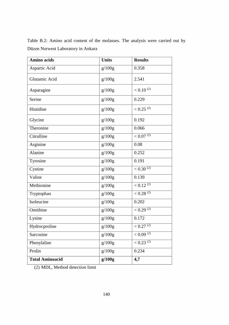
140

Table B.2: Amino acid content of the molasses. The analysis were carried out by

Düzen Norwest Laboratory in Ankara

Amino acids Units Results

Aspartic Acid g/100g 0.358

Glutamic Acid g/100g 2.541

Asparagine g/100g < 0.10 (2)

Serine g/100g 0.229

Histidine g/100g < 0.25 (2)

Glycine g/100g 0.192

Theronine g/100g 0.066

Citrulline g/100g < 0.07 (2)

Arginine g/100g 0.08

Alanine g/100g 0.252

Tyrosine g/100g 0.191

Cystine g/100g < 0.30 (2)

Valine g/100g 0.139

Methionine g/100g < 0.12 (2)

Tryptophan g/100g < 0.28 (2)

Isoleucine g/100g 0.202

Omithine g/100g < 0.29 (2)

Lysine g/100g 0.172

Hydrocproline g/100g < 0.27 (2)

Sarcosine g/100g < 0.09 (2)

Phenylaline g/100g < 0.23 (2)

Prolin g/100g 0.234

Total Aminoacid g/100g 4,7

(2) MDL, Method detection limit

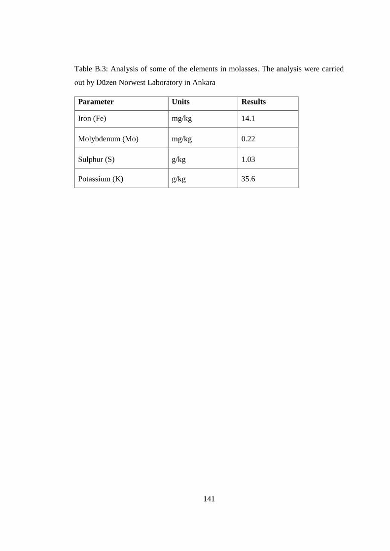
141

Table B.3: Analysis of some of the elements in molasses. The analysis were carried

out by Düzen Norwest Laboratory in Ankara

Parameter Units Results

Iron (Fe) mg/kg 14.1

Molybdenum (Mo) mg/kg 0.22

Sulphur (S) g/kg 1.03

Potassium (K) g/kg 35.6

143

APPENDIX C

DIAMETER SELECTION

C.1. Light Intensity Measurements

In order to determine the light intensity at different depths for different sucrose

concentrations and for different molasses dilution rates, a luxmeter (Extech HD450)

was used. Samples were put into 1 cm thick compartments. Light intensity just in front

of the first compartment was adjusted to 4000 lux. In the first run light that is

penetrated from the empty compartments were measured for 1 cm, 2 cm, 3 cm, 4 cm

and 5 cm thicknesses. Then, solution containing 5 mM sucrose was filled to the

compartments, and light intensity was measured at different thicknesses (1 - 5 cm).

The same procedure was applied for 7.5 mM, 10 mM, 20 mM sucrose concentrations.

Same procedure also applied for different molasses dilution rates (20X, 40X, 60X,

80X and 100X). The results of the experiments are given in Figure C.1, Figure C.2 and

Figure C.3.

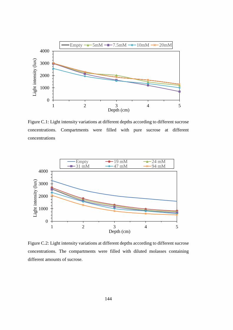
144


concentrations. Compartments were filled with pure sucrose at different

concentrations



different amounts of sucrose.

0

1000

2000

3000

4000

1 2 3 4 5

Lig

ht

inte

nsi

ty (

lux

)

Depth (cm)

Empty 5mM 7.5mM 10mM 20mM

0

1000

2000

3000

4000

1 2 3 4 5

Lig

ht

inte

nsi

ty (

lux

)

Depth (cm)

Empty 19 mM 24 mM31 mM 47 mM 94 mM

145

Figure C.3: Light intensity variation for 3 cm depth according to different sucrose


different amounts of sucrose.

C.2. Photon Count Measurements

Photon count measurements were done by using a spectroradiometer (Spectrawiz EPP

2000). The detector was connected to the spectroradiometer and the spectroradiometer

was connected to a computer as shown in Figure C.4. Data was recorded by the

program named SpectraWiz. The parameters of Spectrawiz are given in Table C. 1.

Figure C.4: Schematic representation of the spectroradiometer

y = 0.0833x2 - 15.774x + 1567.9

R² = 0.9972

400

800

1200

1600

15 35 55 75 95

Lig

ht

inte

nsi

ty (

lux

)

Sucrose concentation (mM)

146

Table C. 1: The parameters used for the spectroradiometer

Detector integration period in milliseconds 7

Number of samples averaged 1

Pixel smoothing 1 = 5 pixels

Temperature compensation on/off off

Timing resolution control 1 = low

Channel 1

Photon count measurements were done for 1 cm, 2 cm, 3 cm, 4 cm and 5 cm thick

empty compartments. Then the same procedure was applied for different sucrose

concentrations and for different molasses dilution rates. The experimental set – up is

shown in Figure C.4. The experiment was performed in a dark room so that the

measurements was not affected by the light coming from other sources. The result is

given in Figure C.5 and Figure C.7.

Figure C.5: Photon counts with respect to wavelength for 19 mM sucrose containing

molasses at different thicknesses

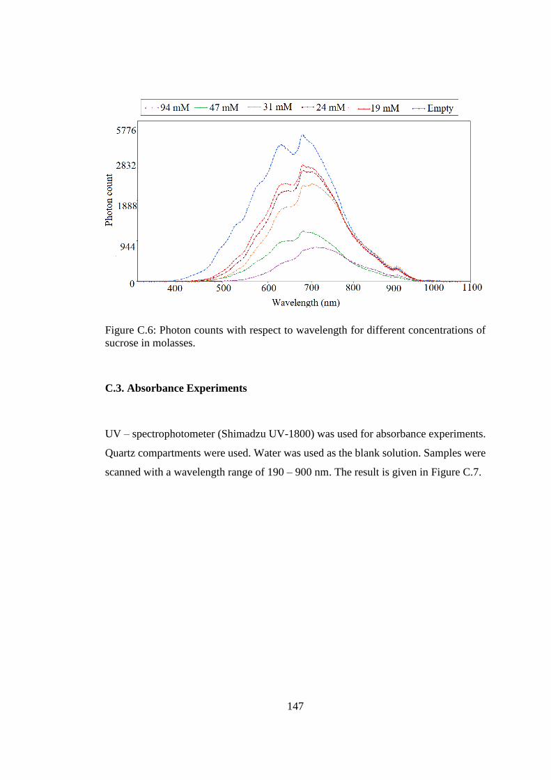
147

Figure C.6: Photon counts with respect to wavelength for different concentrations of

sucrose in molasses.

C.3. Absorbance Experiments

UV – spectrophotometer (Shimadzu UV-1800) was used for absorbance experiments.

Quartz compartments were used. Water was used as the blank solution. Samples were

scanned with a wavelength range of 190 – 900 nm. The result is given in Figure C.7.

148

Figure C.7: Comparison of absorbance values for different molasses dilutions

Table C.2: OD of molasses for different dilutions

Dilution OD at 660 nm

20 X dilution 0.184

40X dilution 0.082

60X dilution 0.073

80X dilution 0.057

100X dilution 0.042

149

APPENDIX D

PUMP SELECTION

D.1. Experimental Procedure for Pump Selection

The bacteria was grown in Biebl and Pfenning medium (Biebl & Pfennig, 1981),

containing 40 mM acetate and 2 mM glutamate. Then the bacteria was adopted to

sucrose in indoor conditions. When the concentration of the bacteria reached to around

0.5 gdcw/L, 10% (v/v) bacteria was inoculated to the previously sterilized U-tube

reactors. During the first day, pH and cell concentration were measured with 1 hour

intervals. 3 measurements for pH and cell concentration were taken, the average values

were reported. The experiment was performed in the green house. The starting date of

the experiment was in December 12, 2014. It lasted for 3 days.

150

D.2. pH variation

Figure D. 1: pH variation for different pump types for the first day. The starting date

of the experiment was Decemeber 12, 2014.

Figure D.2: pH variation for different pump types for the first day. The starting date of

the experiment was Decemeber 12, 2014.

7,3

7,35

7,4

7,45

7,5

7,55

7,6

0 2 4 6 8 10

pH

Time (hour)


6,2

6,4

6,6

6,8

7

7,2

7,4

7,6

7,8

0 10 20 30 40 50 60

pH

Time (hour)


151

D.3. Experimental Data of the Pump Selection

Table D.1: The daily temperature and light intensity change

Date: 28.12.2014

Time Peristaltic pump

System Temp.

(0C)

Aquarium pump

System Temp.

Light Intensity

08:30 10.5 11 3.0 Klux

09:30 15.5 15.5 3.6 Klux

10:30 23.5 24 2.3 Klux

11:30 31 31.5 14 Klux

12:30 34 34.5 67 Klux

13:30 29 29 15 Klux

14:30 23.5 23.5 8.5 Klux

15:30 18.5 18 0.37 Klux

16:30 17 16.5 450 Lux

Date: 29.12.2014

16:30 - - -

Date: 30.12.2014

13:30 18 18 3.25 Klux

16:30 14 13.5 500 Lux

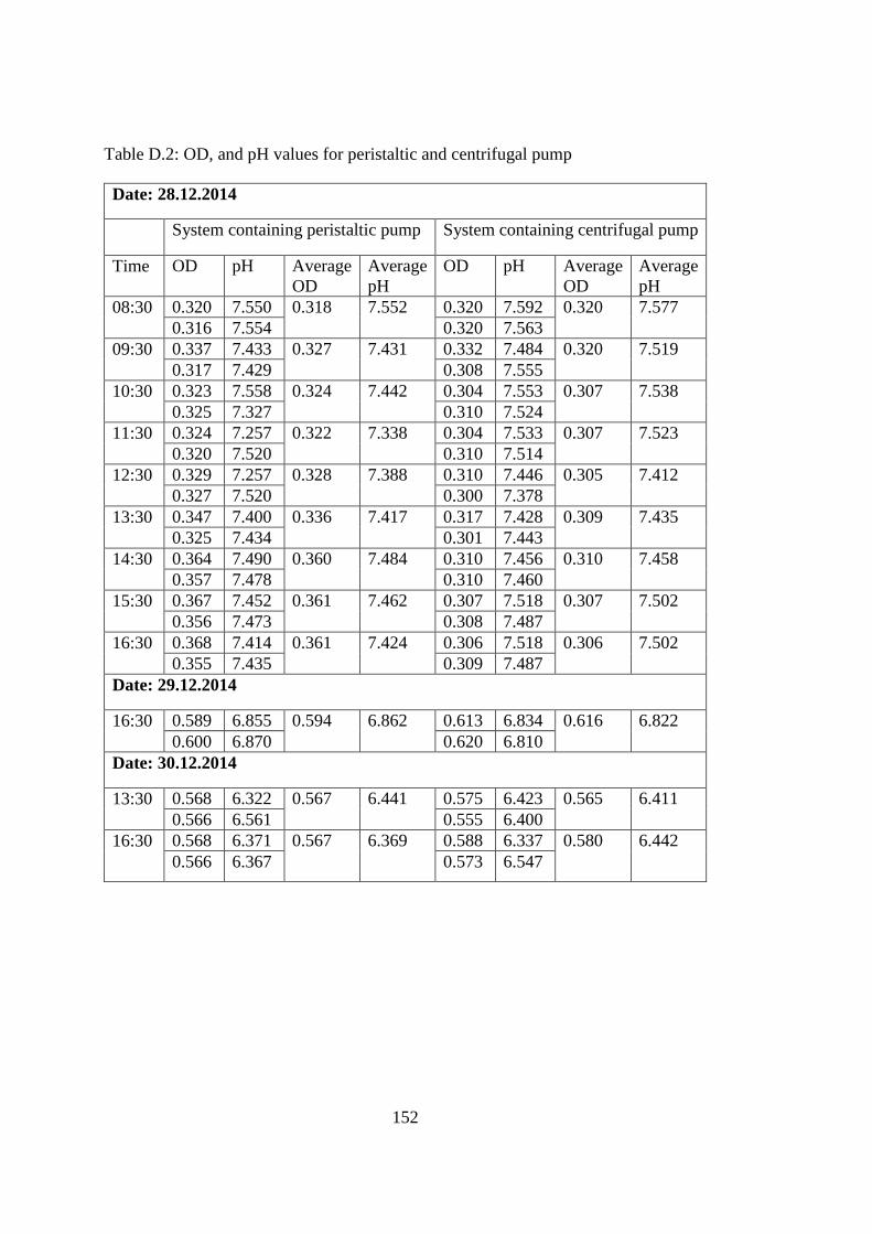
152

Table D.2: OD, and pH values for peristaltic and centrifugal pump

Date: 28.12.2014

System containing peristaltic pump System containing centrifugal pump

Time OD pH Average

OD

Average

pH

OD pH Average

OD

Average

pH

08:30 0.320 7.550 0.318 7.552 0.320 7.592 0.320 7.577

0.316 7.554 0.320 7.563

09:30 0.337 7.433 0.327 7.431 0.332 7.484 0.320 7.519

0.317 7.429 0.308 7.555

10:30 0.323 7.558 0.324 7.442 0.304 7.553 0.307 7.538

0.325 7.327 0.310 7.524

11:30 0.324 7.257 0.322 7.338 0.304 7.533 0.307 7.523

0.320 7.520 0.310 7.514

12:30 0.329 7.257 0.328 7.388 0.310 7.446 0.305 7.412

0.327 7.520 0.300 7.378

13:30 0.347 7.400 0.336 7.417 0.317 7.428 0.309 7.435

0.325 7.434 0.301 7.443

14:30 0.364 7.490 0.360 7.484 0.310 7.456 0.310 7.458

0.357 7.478 0.310 7.460

15:30 0.367 7.452 0.361 7.462 0.307 7.518 0.307 7.502

0.356 7.473 0.308 7.487

16:30 0.368 7.414 0.361 7.424 0.306 7.518 0.306 7.502

0.355 7.435 0.309 7.487

Date: 29.12.2014

16:30 0.589 6.855 0.594 6.862 0.613 6.834 0.616 6.822

0.600 6.870 0.620 6.810

Date: 30.12.2014

13:30 0.568 6.322 0.567 6.441 0.575 6.423 0.565 6.411

0.566 6.561 0.555 6.400

16:30 0.568 6.371 0.567 6.369 0.588 6.337 0.580 6.442

0.566 6.367 0.573 6.547

153

APPENDIX E

CALIBRATION CURVE OF THE DRY CELL WEIGHT

Figure E.1: Calibration curve for the dry cell weight versus OD660 of the Rhodobacter

capsulatus YO3 (hup-) (Öztürk, 2005). Optical density of 1.0 at 660 nm corresponds to

0.4656 gdcw/Lc.

155

APPENDIX F

LIGHT ABSORPTION SPECTRA OF Rhodobacter capsulatus YO3 (hup-)

Figure F.1: Light absroption spectra of Rhodobacter capsulatus YO3 (hup-). Optical

density at 660 nm was 1.4.

157

APPENDIX G

SAMPLE GAS CHROMATOGRAM FOR GAS ANALYSIS

Figure G.1: A sample gas chromotogram (Androga, 2009)

159

APPENDIX H

SAMPLE HPLC CHROMATOGRAM AND CALIBRATION CURVES OF

ORGANIC ACIDS AND SUCROSE

Figure H.1: A sample HPLC chromotogram. (Androga, 2009). Retention times of

lactic, formic, acetic, propionic and butyric acid are 22.0, 24.5, 26.5, 31.3 and 38.6

min, respectively.

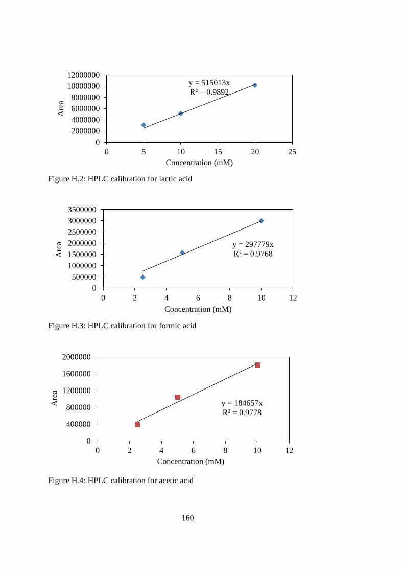
160

Figure H.2: HPLC calibration for lactic acid

Figure H.3: HPLC calibration for formic acid

Figure H.4: HPLC calibration for acetic acid

y = 515013x

R² = 0.9892

0

2000000

4000000

6000000

8000000

10000000

12000000

0 5 10 15 20 25

Are

a

Concentration (mM)

y = 297779x

R² = 0.9768

0

500000

1000000

1500000

2000000

2500000

3000000

3500000

0 2 4 6 8 10 12

Are

a

Concentration (mM)

y = 184657x

R² = 0.9778

0

400000

800000

1200000

1600000

2000000

0 2 4 6 8 10 12

Are

a

Concentration (mM)

161

Figure H.5: HPLC calibration for propionic acid

Figure H.6: HPLC calibration for butyric acid

y = 210262x

R² = 0.9745

0

500000

1000000

1500000

2000000

2500000

0 2 4 6 8 10 12

Are

a

Concentration (mM)

y = 218362x

R² = 0.9737

0

500000

1000000

1500000

2000000

2500000

0 2 4 6 8 10 12

Are

a

Concentration (mM)

163

APPENDIX I

MODEL OUTPUTS

Figure I.1: Velocity profile for 3.8 m tube length, 10.5 cm tube spacing and 25 L/h

volumetric flow rate.

Figure I.2: Pressure profile for 3.8 m tube length, 10.5 cm tube spacing and 25 L/h

volumetric flow rate.

165

APPENDIX J

OUTDOOR EXPERIMENTAL DATA

Table J.1: Daily variation in pH and cell concentration of RUN 092014. The

experiment started on September 10, 2014.

Date Day number pH

Cell

concentration

(gdcw/Lc) ODave

10.09.2014 1 7.14 0.153 0.329

11.09.2014 2 6.47 0.249 0.53525

12.09.2014 3 6.41 0.237 0.5085

13.09.2014 4 6.36 0.256 0.5505

14.09.2014 5 6.49 0.186 0.4

15.09.2014 6 6.46 0.168 0.361

16.09.2014 7 6.43 0.177 0.38

17.09.2014 8 6.34 0.158 0.34

18.09.2014 9 6.37 0.147 0.316

19.09.2014 10 6.40 0.119 0.255

20.09.2014 11 6.48 0.212 0.4545

21.09.2014 12 5.95 0.405 0.86975

22.09.2014 13 5.58 0.406 0.873

23.09.2014 14 5.10 0.463 0.995

24.09.2014 15 4.84 0.423 0.908

25.09.2014 16 4.67 0.391 0.83925

26.09.2014 17 4.61 0.313 0.67275

27.09.2014 18 4.55 0.260 0.55875

28.09.2014 19 4.85 0.259 0.55525

29.09.2014 20 5.14 0.291 0.62425

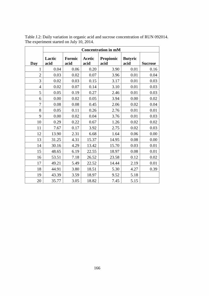
166

Table J.2: Daily variation in organic acid and sucrose concentration of RUN 092014.

The experiment started on July 10, 2014.

Day

Concentration in mM

Lactic

acid

Formic

acid

Acetic

acid

Propionic

acid

Butyric

acid Sucrose

1 0.04 0.06 0.20 3.90 0.01 0.16

2 0.03 0.02 0.07 3.96 0.01 0.04

3 0.02 0.03 0.15 3.17 0.01 0.03

4 0.02 0.07 0.14 3.10 0.01 0.03

5 0.05 0.19 0.27 2.46 0.01 0.03

6 0.00 0.02 0.05 3.94 0.00 0.02

7 0.08 0.08 0.45 2.06 0.02 0.04

8 0.05 0.11 0.26 2.76 0.01 0.01

9 0.00 0.02 0.04 3.76 0.01 0.03

10 0.29 0.22 0.67 1.26 0.02 0.02

11 7.67 0.17 3.92 2.75 0.02 0.03

12 13.90 2.31 6.68 1.64 0.06 0.00

13 31.25 4.31 15.37 14.95 0.08 0.00

14 30.16 4.29 13.42 15.70 0.03 0.01

15 48.65 6.19 22.55 18.97 0.08 0.01

16 53.51 7.18 26.52 23.58 0.12 0.02

17 49.21 5.49 22.52 14.44 2.19 0.01

18 44.91 3.80 18.51 5.30 4.27 0.39

19 43.39 3.59 18.97 9.52 5.18

20 35.77 3.05 18.82 7.45 5.15

167



Date Hour Day OD1 OD2 OD3 ODave

Cell

Conc.

(gdcw/Lc)

12.07.2015 18:30 0.5 0.632 0.632 0.632 0.632 0.294

13.07.2015 0.396 1.0 0.801 0.820 0.814 0.812 0.378

19:30 1.5 1.173 1.195 1.204 1.191 0.554

14.07.2015 08:45 2.0 1.205 1.24 1.257 1.234 0.575

18:00 2.5 1.563 1.577 1.582 1.574 0.733

15.07.2015 08:45 3.0 1.6 1.597 1.625 1.607 0.748

18:30 3.5 1.567 1.555 1.565 1.562 0.727

16.07.2015 09:00 4.0 1.538 1.526 1.529 1.531 0.713

19:00 4.5 1.276 1.28 1.276 1.277 0.595

17.07.2015 09:30 5.0 1.141 1.149 1.155 1.148 0.535

19:00 5.5 1.133 1.134 1.129 1.132 0.527

18.07.2015 08:30 6.0 1.094 1.093 1.097 1.095 0.510

18:30 6.5 1.096 1.108 1.106 1.103 0.514

19.07.2015 08:30 7.0 1.031 1.114 1.129 1.091 0.508

18:30 7.5 1.125 1.131 1.135 1.130 0.526

20.07.2015 08:30 8.0 1.162 1.173 1.172 1.169 0.544

19:00 8.5 1.102 1.102 1.111 1.105 0.514

21.07.2015 08:30 9.0 1.078 1.099 1.096 1.091 0.508

19:00 9.5 1.140 1.150 1.140 1.143 0.532

168

Table J. 4: Daily variation in pH of RUN 072015-R1. The experiment started on July

12, 2015.

Date Hour Day pH1 pH2 pH3

pH-

ave

12.07.2015 18:30 0 6.40 6.40 6.40 6.40

13.07.2015 08:30 0.5 6.54 6.53 6.54 6.54

19:30 1.0 6.70 6.68 6.67 6.68

14.07.2015 08:45 1.5 6.70 6.68 6.67 6.68

18:00 2.0 6.85 6.87 6.88 6.87

15.07.2015 08:45 2.5 6.86 6.92 6.95 6.91

18:30 3.0 6.90 6.89 6.96 6.92

16.07.2015 09:00 3.5 6.93 6.91 6.90 6.91

19:00 4.0 6.83 6.83 6.84 6.83

17.07.2015 09:30 4.5 6.77 6.78 6.84 6.80

19:00 5.0 6.79 6.78 6.79 6.79

18.07.2015 08:30 5.5 6.68 6.73 6.74 6.72

18:30 6.0 6.77 6.76 6.75 6.76

19.07.2015 08:30 6.5 6.74 6.74 6.75 6.74

18:30 7.0 6.48 6.52 6.52 6.51

20.07.2015 08:30 7.5 6.53 6.53 6.54 6.53

19:00 8.0 6.57 6.57 6.57 6.57

21.07.2015 08:30 8.5 6.57 6.59 6.58 6.58

19:00 9.0 6.58 6.58 6.58 6.58

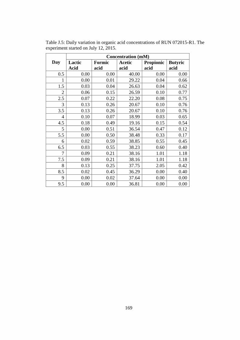
169

Table J.5: Daily variation in organic acid concentrations of RUN 072015-R1. The

experiment started on July 12, 2015.

Day

Concentration (mM)

Lactic

Acid

Formic

acid

Acetic

acid

Propionic

acid

Butyric

acid

0.5 0.00 0.00 40.00 0.00 0.00

1 0.00 0.01 29.22 0.04 0.66

1.5 0.03 0.04 26.63 0.04 0.62

2 0.06 0.15 26.59 0.10 0.77

2.5 0.07 0.22 22.20 0.08 0.75

3 0.13 0.26 20.67 0.10 0.76

3.5 0.13 0.26 20.67 0.10 0.76

4 0.10 0.07 18.99 0.03 0.65

4.5 0.18 0.49 19.16 0.15 0.54

5 0.00 0.51 36.54 0.47 0.12

5.5 0.00 0.50 38.48 0.33 0.17

6 0.02 0.59 38.85 0.55 0.45

6.5 0.03 0.55 38.23 0.60 0.40

7 0.09 0.21 38.16 1.01 1.18

7.5 0.09 0.21 38.16 1.01 1.18

8 0.13 0.25 37.75 2.05 0.42

8.5 0.02 0.45 36.29 0.00 0.40

9 0.00 0.02 37.64 0.00 0.00

9.5 0.00 0.00 36.81 0.00 0.00

170

Table J. 6: Biogas production of RUN 072015-R1. The experiment started on July 12,

2015.

Date Day

H2

%

CO2

%

Total

gas

(mL)

Daily H2

produce

d (mol)

H2

productivity

(mol/(m3.h)

Daily

solar

radiation

(W/m2)

13.07.

2015 1 96.8 3.2 171 0.006 0.038 248.63

14.07.

2015 2 96.5 3.5 643 0.022 0.144 325.970

15.07.

2015 3 97.6 2.4 372 0.013 0.084 297.760

16.07.

2015 4 95.8 4.2 556 0.019 0.123 291.350

17.07.

2015 5 93.0 7.0 165 0.005 0.036 322.201

18.07.

2015 6 78.7 21.3 239 0.007 0.044 323.550

19.07.

2015 7 87.2 12.8 429 0.013 0.087 327.940

20.07.

2015 8 87.5 12.5 301 0.009 0.061 327.960

21.07.

2015 9 6.5 93.5 2 0.000 0.000 328.530

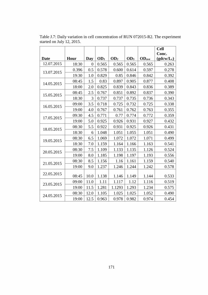
171



Date Hour Day OD1 OD2 OD3 ODave

Cell

Conc.

(gdcw/Lc)

12.07.2015 18:30 0 0.565 0.565 0.565 0.565 0.263

13.07.2015 0.396 0.5 0.578 0.600 0.614 0.597 0.278

19:30 1.0 0.829 0.85 0.846 0.842 0.392

14.05.2015 08:45 1.5 0.83 0.897 0.905 0.877 0.408

18:00 2.0 0.825 0.839 0.843 0.836 0.389

15.05.2015 08:45 2.5 0.767 0.851 0.892 0.837 0.390

18:30 3 0.737 0.737 0.735 0.736 0.343

16.05.2015 09:00 3.5 0.718 0.725 0.732 0.725 0.338

19:00 4.0 0.767 0.761 0.762 0.763 0.355

17.05.2015 09:30 4.5 0.771 0.77 0.774 0.772 0.359

19:00 5.0 0.925 0.926 0.931 0.927 0.432

18.05.2015 08:30 5.5 0.922 0.931 0.925 0.926 0.431

18:30 6 1.048 1.051 1.055 1.051 0.490

19.05.2015 08:30 6.5 1.069 1.072 1.072 1.071 0.499

18:30 7.0 1.159 1.164 1.166 1.163 0.541

20.05.2015 08:30 7.5 1.109 1.133 1.135 1.126 0.524

19:00 8.0 1.185 1.198 1.197 1.193 0.556

21.05.2015 08:30 8.5 1.156 1.16 1.161 1.159 0.540

19:00 9.0 1.237 1.246 1.244 1.242 0.578

22.05.2015 08:45 10.0 1.138 1.146 1.149 1.144 0.533

23.05.2015 09:00 11.0 1.11 1.117 1.12 1.116 0.519

19:00 11.5 1.281 1.1293 1.293 1.234 0.575

24.05.2015 08:30 12.0 1.105 1.025 1.025 1.052 0.490

19:00 12.5 0.963 0.978 0.982 0.974 0.454

172

Table J.8: Daily variation in pH of RUN 072015-R2. The experiment started on July

12, 2015.

Date Hour Day pH1 pH2 pH3

pH-

ave

12.07.2015 18:30 0 7.500 7.500 7.500 7.500

13.07.2015 0.396 0.5 7.310 7.300 7.300 7.303

19:30 1.0 6.4 6.41 6.42 6.410

14.05.2015 08:45 1.5 6.4 6.39 6.4 6.397

18:00 2.0 6.43 6.40 6.41 6.41

15.05.2015 08:45 2.5 6.38 6.42 6.45 6.42

18:30 3 6.40 6.39 6.39 6.39

16.05.2015 09:00 3.5 6.43 6.40 6.39 6.41

19:00 4.0 6.43 6.43 6.43 6.43

17.05.2015 09:30 4.5 6.41 6.40 6.42 6.41

19:00 5.0 6.08 6.08 6.07 6.08

18.05.2015 08:30 5.5 6.05 6.06 6.05 6.05

18:30 6 5.93 5.96 5.96 5.95

19.05.2015 08:30 6.5 5.95 5.95 5.97 5.96

18:30 7.0 5.94 5.93 5.93 5.93

20.05.2015 08:30 7.5 6.00 6.00 5.99 6.00

19:00 8.0 5.98 5.97 5.99 5.98

21.05.2015 08:30 8.5 5.99 6.01 6.02 6.01

19:00 9 5.95 5.98 5.99 5.97

22.05.2015 08:45 9.5 6.01 6.00 6.02 6.01

23.05.2015 09:00 10.5 5.94 5.98 5.97 5.96

19:00 11.0 5.94 5.92 5.93 5.93

24.05.2015 08:30 11.5 5.97 5.92 5.93 5.94

19:00 12 5.77 5.76 5.76 5.76

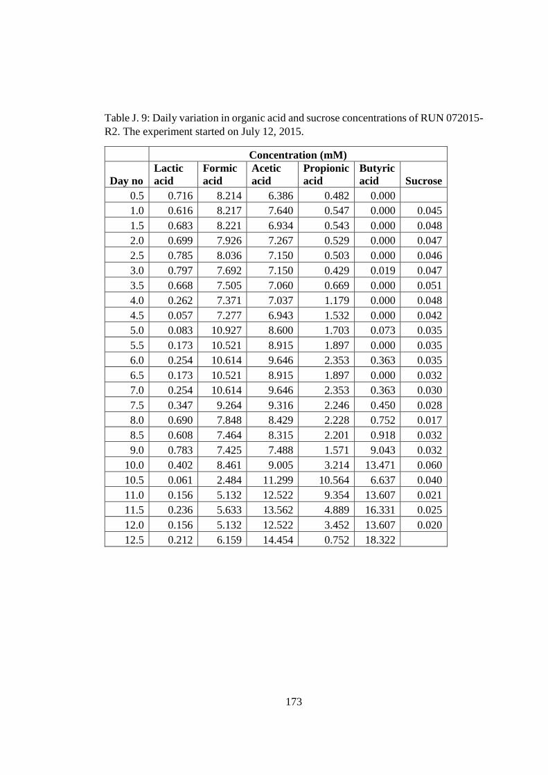
173

Table J. 9: Daily variation in organic acid and sucrose concentrations of RUN 072015-

R2. The experiment started on July 12, 2015.

Concentration (mM)

Day no

Lactic

acid

Formic

acid

Acetic

acid

Propionic

acid

Butyric

acid Sucrose

0.5 0.716 8.214 6.386 0.482 0.000

1.0 0.616 8.217 7.640 0.547 0.000 0.045

1.5 0.683 8.221 6.934 0.543 0.000 0.048

2.0 0.699 7.926 7.267 0.529 0.000 0.047

2.5 0.785 8.036 7.150 0.503 0.000 0.046

3.0 0.797 7.692 7.150 0.429 0.019 0.047

3.5 0.668 7.505 7.060 0.669 0.000 0.051

4.0 0.262 7.371 7.037 1.179 0.000 0.048

4.5 0.057 7.277 6.943 1.532 0.000 0.042

5.0 0.083 10.927 8.600 1.703 0.073 0.035

5.5 0.173 10.521 8.915 1.897 0.000 0.035

6.0 0.254 10.614 9.646 2.353 0.363 0.035

6.5 0.173 10.521 8.915 1.897 0.000 0.032

7.0 0.254 10.614 9.646 2.353 0.363 0.030

7.5 0.347 9.264 9.316 2.246 0.450 0.028

8.0 0.690 7.848 8.429 2.228 0.752 0.017

8.5 0.608 7.464 8.315 2.201 0.918 0.032

9.0 0.783 7.425 7.488 1.571 9.043 0.032

10.0 0.402 8.461 9.005 3.214 13.471 0.060

10.5 0.061 2.484 11.299 10.564 6.637 0.040

11.0 0.156 5.132 12.522 9.354 13.607 0.021

11.5 0.236 5.633 13.562 4.889 16.331 0.025

12.0 0.156 5.132 12.522 3.452 13.607 0.020

12.5 0.212 6.159 14.454 0.752 18.322

174

Table J.10: Biogas production of RUN 072015-R2. The experiment started on July

12, 2015.

Date

Gas content Total

gas

(mL)

H2

produce

d (mol)

H2

productivity

(mol

H2/(m3.h)

Daily solar

radiation

(W/m2)

H2%

CO2

%

13.07.2015 0.0 0.0 0.0 0.000 0.000 248.63

14.07.2015 0.0 0.0 0.0 0.000 0.000 325.970

15.07.2015 100.0 0.0 18 0.001 0.005 297.760

16.07.2015 0.0 0.0 0.0 0.000 0.000 291.350

17.07.2015 84.7 15.3 532 0.016 0.128 322.201

18.07.2015 53.5 46.5 506 0.010 0.077 323.550

19.07.2015 37.5 62.5 1484 0.020 0.158 327.940

20.07.2015 24.5 75.5 1865 0.016 0.129 327.960

21.07.2015 29.6 70.4 1298 0.014 0.109 328.530

22.07.2015 23.2 76.8 4732 0.039 0.311 326.900

23.07.2015 20.2 79.8 3851 0.028 0.220 320.450

24.07.2015 17.6 82.4 3090 0.019 0.155 319.270

Table J.11: Data taken from the weather station on July 21, 2015.

Time Air

Temperatur

e (oC)

Humidit

y

Dew

Poin

t

(oC)

Win

d

Spee

d

(m/s)

Heat

Inde

x

Pressur

e

Solar

Radiatio

n (W/m2)

12:00

AM

15.3 40 1.8 3.2 13.8 1006.5 0

12:05

AM

15.1 41 1.9 3.2 13.7 1006.5 0

12:10

AM

15.1 41 1.9 3.2 13.7 1006.5 0

12:15

AM

15 41 1.8 3.2 13.6 1006.6 0

12:20

AM

14.8 43 2.4 1.6 13.5 1006.5 0

12:25

AM

14.8 43 2.4 1.6 13.5 1006.6 0

12:30

AM

15.1 43 2.6 1.6 13.7 1006.5 0

12:35

AM

15.3 43 2.8 1.6 13.9 1006.6 0

12:40

AM

15.7 43 3.2 1.6 14.3 1006.5 0

175

Table J.11.continued

12:50 AM 16 44 3.7 1.6 14.7 1006.5 0

12:55 AM 15.9 45 4 1.6 14.6 1006.5 0

1:00 AM 15.6 44 3.4 1.6 14.3 1006.5 0

1:05 AM 15.8 44 3.6 3.2 14.5 1006.5 0

1:10 AM 15.9 45 4 3.2 14.6 1006.6 0

1:15 AM 15.5 47 4.2 1.6 14.3 1006.6 0

1:20 AM 14.9 48 4 1.6 13.8 1006.6 0

1:25 AM 14.4 50 4.1 1.6 13.3 1006.5 0

1:30 AM 14.1 51 4.1 1.6 13 1006.5 0

1:35 AM 13.8 52 4.1 3.2 12.8 1006.5 0

1:40 AM 13.8 51 3.8 3.2 12.8 1006.5 0

1:45 AM 13.6 52 3.9 3.2 12.6 1006.6 0

1:50 AM 13.6 53 4.1 3.2 12.6 1006.6 0

1:55 AM 13.4 53 4 3.2 12.4 1006.5 0

2:00 AM 13.2 54 4.1 1.6 12.3 1006.6 0

2:05 AM 13.2 54 4.1 3.2 12.3 1006.6 0

2:10 AM 13.2 54 4.1 3.2 12.3 1006.7 0

2:15 AM 13.3 54 4.2 3.2 12.4 1006.6 0

2:20 AM 13.3 54 4.2 3.2 12.4 1006.6 0

2:25 AM 13.2 54 4.1 3.2 12.3 1006.7 0

2:30 AM 13.1 55 4.3 3.2 12.2 1006.7 0

2:35 AM 13.2 55 4.3 3.2 12.3 1006.7 0

2:40 AM 13.1 55 4.3 3.2 12.2 1006.8 0

2:45 AM 13.1 55 4.3 3.2 12.2 1006.9 0

2:50 AM 13.4 54 4.3 1.6 12.4 1006.9 0

2:55 AM 13.8 54 4.6 4.8 12.8 1006.9 0

3:00 AM 14.3 53 4.8 3.2 13.3 1006.8 0

3:05 AM 14.4 53 5 0 13.4 1006.8 0

3:10 AM 14.1 54 4.9 1.6 13.2 1006.8 0

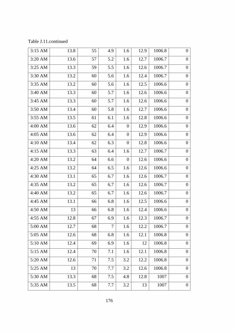
176


3:15 AM 13.8 55 4.9 1.6 12.9 1006.8 0

3:20 AM 13.6 57 5.2 1.6 12.7 1006.7 0

3:25 AM 13.3 59 5.5 1.6 12.6 1006.7 0

3:30 AM 13.2 60 5.6 1.6 12.4 1006.7 0

3:35 AM 13.2 60 5.6 1.6 12.5 1006.6 0

3:40 AM 13.3 60 5.7 1.6 12.6 1006.6 0

3:45 AM 13.3 60 5.7 1.6 12.6 1006.6 0

3:50 AM 13.4 60 5.8 1.6 12.7 1006.6 0

3:55 AM 13.5 61 6.1 1.6 12.8 1006.6 0

4:00 AM 13.6 62 6.4 0 12.9 1006.6 0

4:05 AM 13.6 62 6.4 0 12.9 1006.6 0

4:10 AM 13.4 62 6.3 0 12.8 1006.6 0

4:15 AM 13.3 63 6.4 1.6 12.7 1006.7 0

4:20 AM 13.2 64 6.6 0 12.6 1006.6 0

4:25 AM 13.2 64 6.5 1.6 12.6 1006.6 0

4:30 AM 13.1 65 6.7 1.6 12.6 1006.7 0

4:35 AM 13.2 65 6.7 1.6 12.6 1006.7 0

4:40 AM 13.2 65 6.7 1.6 12.6 1006.7 0

4:45 AM 13.1 66 6.8 1.6 12.5 1006.6 0

4:50 AM 13 66 6.8 1.6 12.4 1006.6 0

4:55 AM 12.8 67 6.9 1.6 12.3 1006.7 0

5:00 AM 12.7 68 7 1.6 12.2 1006.7 0

5:05 AM 12.6 68 6.8 1.6 12.1 1006.8 0

5:10 AM 12.4 69 6.9 1.6 12 1006.8 0

5:15 AM 12.4 70 7.1 1.6 12.1 1006.8 0

5:20 AM 12.6 71 7.5 3.2 12.2 1006.8 0

5:25 AM 13 70 7.7 3.2 12.6 1006.8 0

5:30 AM 13.3 68 7.5 4.8 12.8 1007 0

5:35 AM 13.5 68 7.7 3.2 13 1007 0

177


5:40 AM 13.4 68 7.6 3.2 12.9 1007.1 5

5:45 AM 13.2 68 7.4 1.6 12.7 1007 7

5:50 AM 13.1 69 7.5 1.6 12.7 1007.1 10

5:55 AM 13.1 69 7.5 1.6 12.6 1007.1 13

6:00 AM 13.1 70 7.7 1.6 12.6 1007.2 15

6:05 AM 13.2 70 7.9 1.6 12.8 1007.1 19

6:10 AM 13.4 71 8.3 0 13 1007.2 25

6:15 AM 13.7 70 8.3 1.6 13.2 1007.1 31

6:20 AM 14.2 69 8.6 1.6 13.7 1007.2 40

6:25 AM 14.7 68 8.9 3.2 14.3 1007.2 50

6:30 AM 15.3 68 9.5 1.6 14.9 1007.2 61

6:35 AM 15.9 67 9.8 1.6 15.6 1007.2 75

6:40 AM 16.5 65 9.9 1.6 16.1 1007.3 89

6:45 AM 17.2 64 10.3 0 16.8 1007.3 105

6:50 AM 17.9 60 10 0 17.4 1007.3 116

6:55 AM 18.5 59 10.3 1.6 18 1007.2 123

7:00 AM 19.2 60 11.3 0 18.9 1007.3 132

7:05 AM 19.9 51 9.4 0 19.2 1007.3 151

7:10 AM 20.6 47 8.8 1.6 19.6 1007.3 182

7:15 AM 20.9 49 9.8 1.6 20 1007.2 214

7:20 AM 21.2 47 9.4 1.6 20.1 1007.1 231

7:25 AM 21.6 47 9.8 0 20.7 1007.2 247

7:30 AM 22 46 9.8 1.6 21.2 1007.3 264

7:35 AM 22.3 45 9.8 1.6 21.6 1007.1 281

7:40 AM 22.3 45 9.8 1.6 21.6 1007.1 299

7:45 AM 22.7 44 9.8 1.6 22.1 1007.1 316

7:50 AM 22.8 43 9.6 1.6 22.3 1007.1 326

7:55 AM 22.8 43 9.6 3.2 22.3 1007 324

8:00 AM 22.7 45 10.1 3.2 22.1 1007.2 338

178


8:05 AM 22.7 45 10.1 1.6 22.1 1007.1 378

8:10 AM 22.6 43 9.4 3.2 21.9 1007 399

8:15 AM 22.6 43 9.4 1.6 21.9 1007 415

8:20 AM 22.9 44 10 1.6 22.4 1007 432

8:25 AM 23.3 42 9.7 1.6 22.9 1007 448

8:30 AM 23.8 41 9.7 1.6 23.4 1007 459

8:35 AM 23.9 40 9.5 3.2 23.5 1007 462

8:40 AM 24.2 40 9.7 1.6 23.7 1007 460

8:45 AM 24.4 40 10 1.6 23.9 1007 454

8:50 AM 24.7 39 9.8 1.6 24.2 1006.9 446

8:55 AM 24.9 37 9.2 3.2 24.3 1007 439

9:00 AM 24.9 38 9.6 3.2 24.4 1007 441

9:05 AM 25.2 37 9.4 1.6 24.6 1006.9 451

9:10 AM 25.3 36 9.2 3.2 24.7 1006.9 469

9:15 AM 25.4 36 9.3 1.6 24.8 1006.8 504

9:20 AM 25.8 36 9.6 1.6 25.2 1006.8 546

9:25 AM 25.8 34 8.8 4.8 25.1 1006.9 594

9:30 AM 25.6 36 9.4 3.2 24.9 1006.9 632

9:35 AM 25.7 35 9.1 3.2 24.9 1006.9 658

9:40 AM 25.7 34 8.7 4.8 25 1007 674

9:45 AM 25.9 32 8 4.8 25.1 1007 691

9:50 AM 26.2 32 8.2 3.2 25.3 1006.9 706

9:55 AM 26.6 31 8.1 3.2 25.6 1007 721

10:00 AM 26.9 30 7.9 3.2 25.8 1007 733

10:05 AM 27.1 31 8.5 3.2 26 1006.9 745

10:10 AM 27.3 30 8.2 3.2 26.2 1007 763

10:15 AM 27.3 28 7.2 4.8 26.1 1007 775

10:20 AM 27.3 28 7.2 3.2 26.1 1006.9 792

10:25 AM 27.5 26 6.3 8 26.2 1006.9 801

179


10:30 AM 27.2 26 6 8 25.8 1006.9 812

10:35 AM 27.1 28 7 4.8 25.9 1006.9 825

10:40 AM 27.6 27 6.9 4.8 26.3 1007 836

10:45 AM 27.8 28 7.6 3.2 26.6 1006.9 844

10:50 AM 27.9 27 7.2 4.8 26.7 1006.9 857

10:55 AM 28.2 26 6.9 4.8 26.8 1006.9 868

11:00 AM 27.9 26 6.6 6.4 26.6 1006.9 875

11:05 AM 28 27 7.3 4.8 26.7 1006.8 883

11:10 AM 28.1 27 7.3 4.8 26.8 1006.8 890

11:15 AM 28.2 27 7.4 4.8 26.9 1006.8 892

11:20 AM 28.8 27 7.9 3.2 27.6 1006.7 901

11:25 AM 29.3 24 6.7 3.2 27.8 1006.7 909

11:30 AM 29.4 23 6.1 4.8 27.9 1006.7 919

11:35 AM 29.1 23 5.8 4.8 27.6 1006.7 925

11:40 AM 28.8 22 5 3.2 27.3 1006.6 928

11:45 AM 29 20 3.8 4.8 27.3 1006.6 935

11:50 AM 29.2 19 3.2 3.2 27.4 1006.6 950

11:55 AM 29.3 20 4 4.8 27.6 1006.6 950

12:00 PM 29.4 18 2.6 3.2 27.7 1006.6 954

12:05 PM 29.8 20 4.4 4.8 28.1 1006.6 956

12:10 PM 30.1 18 3.1 3.2 28.2 1006.6 962

12:15 PM 30.1 19 3.9 4.8 28.2 1006.6 965

12:20 PM 30.1 20 4.6 4.8 28.3 1006.5 967

12:25 PM 30 22 6 4.8 28.3 1006.6 969

12:30 PM 29.9 21 5.2 6.4 28.2 1006.5 970

12:35 PM 30.2 21 5.5 3.2 28.5 1006.5 974

12:40 PM 30.3 21 5.6 6.4 28.6 1006.3 975

12:45 PM 30.4 21 5.7 4.8 28.7 1006.4 971

12:50 PM 30.8 21 6 3.2 29 1006.4 973

180


12:55 PM 31 18 3.9 4.8 28.9 1006.4 975

1:00 PM 31 18 3.9 4.8 28.9 1006.3 976

1:05 PM 31.1 20 5.5 4.8 29.1 1006.3 969

1:10 PM 31.4 18 4.3 4.8 29.2 1006.3 972

1:15 PM 31.7 16 2.8 6.4 29.3 1006.3 977

1:20 PM 31.3 16 2.5 8 29 1006.3 976

1:25 PM 31.4 15 1.7 3.2 29 1006.2 975

1:30 PM 31.8 16 2.9 3.2 29.4 1006.2 972

1:35 PM 31.7 16 2.8 6.4 29.2 1006.2 970

1:40 PM 31.8 18 4.5 4.8 29.6 1006.2 963

1:45 PM 31.8 17 3.7 4.8 29.4 1006.1 960

1:50 PM 31.9 16 2.9 4.8 29.6 1006.1 958

1:55 PM 31.8 15 1.9 8 29.3 1006.3 956

2:00 PM 31.9 17 3.8 4.8 29.7 1006.2 949

2:05 PM 32.6 16 3.5 3.2 30.6 1006.1 946

2:10 PM 32.6 15 2.6 6.4 30.4 1006.1 945

2:15 PM 32.7 15 2.7 4.8 30.6 1006.1 940

2:20 PM 32.4 15 2.5 4.8 30.3 1006.2 937

2:25 PM 32.4 13 0.5 4.8 30.2 1006.1 931

2:30 PM 32.3 12 -0.7 4.8 30 1006.2 919

2:35 PM 32.3 12 -0.7 4.8 30 1006.2 918

2:40 PM 32.3 12 -0.7 4.8 30 1006 903

2:45 PM 32.1 11 -2.1 8 29.6 1006.1 902

2:50 PM 32.1 11 -2.1 6.4 29.6 1006.2 890

2:55 PM 32.1 11 -2.1 6.4 29.5 1006.2 885

3:00 PM 32.1 12 -0.9 6.4 29.7 1006.2 872

3:05 PM 31.9 14 1.1 8 29.6 1006.2 859

3:10 PM 32.3 14 1.4 3.2 30.1 1006.1 849

3:15 PM 32.3 14 1.4 4.8 30.2 1006 836

181


3:20 PM 32.4 14 1.5 3.2 30.2 1006 823

3:25 PM 32.3 15 2.4 8 30.2 1005.9 810

3:30 PM 32.4 15 2.5 4.8 30.3 1005.9 798

3:35 PM 32.6 15 2.6 3.2 30.5 1005.9 416

3:40 PM 32.9 14 1.9 3.2 30.7 1005.9 147

3:45 PM 32.8 16 3.7 4.8 30.8 1005.9 65

3:50 PM 32.3 16 3.3 4.8 30.3 1005.7 96

3:55 PM 32.2 16 3.2 6.4 30.2 1005.8 203

4:00 PM 32.1 17 3.9 9.7 29.9 1005.6 496

4:05 PM 32 18 4.7 9.7 29.9 1005.7 691

4:10 PM 32.1 17 4 6.4 30 1005.6 683

4:15 PM 32.3 16 3.3 4.8 30.2 1005.6 675

4:20 PM 32.3 16 3.3 6.4 30.2 1005.6 659

4:25 PM 32.4 16 3.3 4.8 30.3 1005.5 642

4:30 PM 32.4 16 3.4 6.4 30.4 1005.4 628

4:35 PM 32.7 14 1.7 6.4 30.4 1005.5 619

4:40 PM 32.6 13 0.6 6.4 30.3 1005.5 606

4:45 PM 32.4 13 0.4 8 30.1 1005.5 592

4:50 PM 32.3 13 0.4 8 30.1 1005.5 577

4:55 PM 32.4 14 1.5 6.4 30.3 1005.5 559

5:00 PM 32.6 13 0.6 6.4 30.3 1005.5 544

5:05 PM 32.7 13 0.7 4.8 30.4 1005.6 531

5:10 PM 32.6 12 -0.5 8 30.2 1005.6 517

5:15 PM 32.2 13 0.3 9.7 29.9 1005.6 498

5:20 PM 32.1 13 0.2 6.4 29.7 1005.6 483

5:25 PM 32 13 0.1 6.4 29.6 1005.6 465

5:30 PM 32 13 0.1 6.4 29.6 1005.6 449

5:35 PM 31.9 13 0.1 8 29.4 1005.7 432

5:40 PM 31.9 13 0 6.4 29.3 1005.6 416

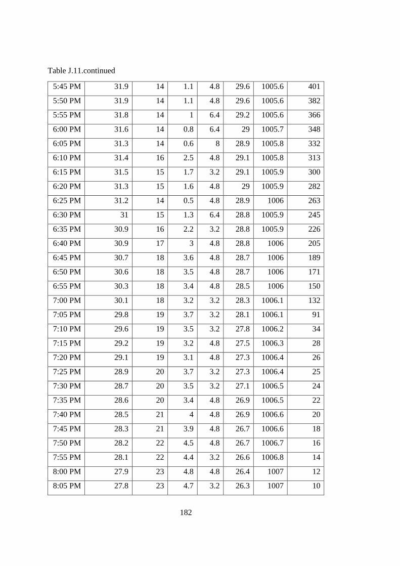
182


5:45 PM 31.9 14 1.1 4.8 29.6 1005.6 401

5:50 PM 31.9 14 1.1 4.8 29.6 1005.6 382

5:55 PM 31.8 14 1 6.4 29.2 1005.6 366

6:00 PM 31.6 14 0.8 6.4 29 1005.7 348

6:05 PM 31.3 14 0.6 8 28.9 1005.8 332

6:10 PM 31.4 16 2.5 4.8 29.1 1005.8 313

6:15 PM 31.5 15 1.7 3.2 29.1 1005.9 300

6:20 PM 31.3 15 1.6 4.8 29 1005.9 282

6:25 PM 31.2 14 0.5 4.8 28.9 1006 263

6:30 PM 31 15 1.3 6.4 28.8 1005.9 245

6:35 PM 30.9 16 2.2 3.2 28.8 1005.9 226

6:40 PM 30.9 17 3 4.8 28.8 1006 205

6:45 PM 30.7 18 3.6 4.8 28.7 1006 189

6:50 PM 30.6 18 3.5 4.8 28.7 1006 171

6:55 PM 30.3 18 3.4 4.8 28.5 1006 150

7:00 PM 30.1 18 3.2 3.2 28.3 1006.1 132

7:05 PM 29.8 19 3.7 3.2 28.1 1006.1 91

7:10 PM 29.6 19 3.5 3.2 27.8 1006.2 34

7:15 PM 29.2 19 3.2 4.8 27.5 1006.3 28

7:20 PM 29.1 19 3.1 4.8 27.3 1006.4 26

7:25 PM 28.9 20 3.7 3.2 27.3 1006.4 25

7:30 PM 28.7 20 3.5 3.2 27.1 1006.5 24

7:35 PM 28.6 20 3.4 4.8 26.9 1006.5 22

7:40 PM 28.5 21 4 4.8 26.9 1006.6 20

7:45 PM 28.3 21 3.9 4.8 26.7 1006.6 18

7:50 PM 28.2 22 4.5 4.8 26.7 1006.7 16

7:55 PM 28.1 22 4.4 3.2 26.6 1006.8 14

8:00 PM 27.9 23 4.8 4.8 26.4 1007 12

8:05 PM 27.8 23 4.7 3.2 26.3 1007 10

183


8:10 PM 27.6 24 5.2 1.6 26.1 1007 6

8:15 PM 27.3 25 5.5 1.6 25.8 1007.1 3

8:20 PM 27 25 5.3 1.6 25.6 1007.1 0

8:25 PM 26.8 26 5.7 1.6 25.4 1007.3 0

8:30 PM 26.6 27 6 0 25.3 1007.3 0

8:35 PM 26 28 6.1 1.6 24.9 1007.4 0

8:40 PM 25.5 29 6.2 1.6 24.6 1007.4 0

8:45 PM 25.2 29 5.9 0 24.4 1007.5 0

8:50 PM 25.1 30 6.3 0 24.4 1007.6 0

8:55 PM 24.7 31 6.4 1.6 23.9 1007.7 0

9:00 PM 23.9 33 6.6 1.6 23.1 1007.8 0

9:05 PM 23.1 35 6.8 1.6 22.3 1007.9 0

9:10 PM 22.6 36 6.8 1.6 21.6 1007.9 0

9:15 PM 22.9 37 7.4 3.2 22.1 1008.1 0

9:20 PM 23.6 36 7.6 1.6 22.9 1008.1 0

9:25 PM 23.9 35 7.5 1.6 23.3 1008.2 0

9:30 PM 24.1 36 8.1 1.6 23.5 1008.4 0

9:35 PM 24 36 8 1.6 23.4 1008.4 0

9:40 PM 23.8 37 8.2 0 23.2 1008.5 0

9:45 PM 23.3 38 8.2 1.6 22.7 1008.6 0

9:50 PM 22.7 40 8.4 1.6 21.9 1008.6 0

9:55 PM 22.6 42 9 1.6 21.9 1008.7 0

10:00 PM 23.2 41 9.2 3.2 22.6 1008.7 0

10:05 PM 23.6 41 9.5 1.6 23.1 1008.7 0

10:10 PM 23.7 41 9.6 1.6 23.2 1008.7 0

10:15 PM 23.6 41 9.6 1.6 23.2 1008.8 0

10:20 PM 23.1 42 9.5 1.6 22.6 1008.8 0

10:25 PM 22.5 44 9.6 1.6 21.8 1008.9 0

10:30 PM 22.5 45 10 1.6 21.8 1008.9 0

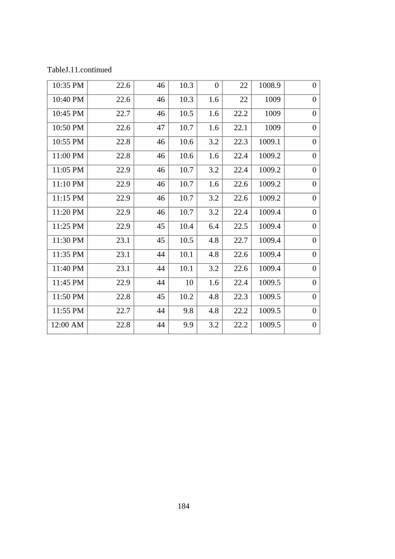
184

TableJ.11.continued

10:35 PM 22.6 46 10.3 0 22 1008.9 0

10:40 PM 22.6 46 10.3 1.6 22 1009 0

10:45 PM 22.7 46 10.5 1.6 22.2 1009 0

10:50 PM 22.6 47 10.7 1.6 22.1 1009 0

10:55 PM 22.8 46 10.6 3.2 22.3 1009.1 0

11:00 PM 22.8 46 10.6 1.6 22.4 1009.2 0

11:05 PM 22.9 46 10.7 3.2 22.4 1009.2 0

11:10 PM 22.9 46 10.7 1.6 22.6 1009.2 0

11:15 PM 22.9 46 10.7 3.2 22.6 1009.2 0

11:20 PM 22.9 46 10.7 3.2 22.4 1009.4 0

11:25 PM 22.9 45 10.4 6.4 22.5 1009.4 0

11:30 PM 23.1 45 10.5 4.8 22.7 1009.4 0

11:35 PM 23.1 44 10.1 4.8 22.6 1009.4 0

11:40 PM 23.1 44 10.1 3.2 22.6 1009.4 0

11:45 PM 22.9 44 10 1.6 22.4 1009.5 0

11:50 PM 22.8 45 10.2 4.8 22.3 1009.5 0

11:55 PM 22.7 44 9.8 4.8 22.2 1009.5 0

12:00 AM 22.8 44 9.9 3.2 22.2 1009.5 0

185

Table J.12: Temperature data taken on July 21, 2015.

Hour

(min)

Reactor 2 Reactor 1

T4 T12 T1 T2 T3 T4 T5 T6 T7 T8 T1 T2 T3 T4 T9 T10 T11 T12

0 17.7 18.9 17.1 17.3 18.2 19.4 19.0 18.9 18.3 19.4 17.1 17.3 18.2 19.4 17.2 17.3 16.6 17.0

10 16.1 18.0 16.5 16.1 16.7 18.7 18.2 18.1 17.5 18.5 16.5 16.1 16.7 18.7 16.1 16.1 15.5 15.7

20 15.5 17.2 16.1 15.4 16.2 17.8 17.4 17.2 16.7 17.6 16.1 15.4 16.2 17.8 15.2 15.4 14.7 15.0

30 15.3 16.8 15.9 14.7 15.8 17.0 16.7 16.5 16.0 16.9 15.9 14.7 15.8 17.0 14.7 14.7 14.1 14.4

40 14.6 16.2 15.6 14.5 15.2 16.3 16.1 15.9 15.3 16.3 15.6 14.5 15.2 16.3 14.3 14.5 13.9 14.1

50 14.5 15.7 15.6 14.3 15.0 15.7 15.6 15.4 14.9 15.8 15.6 14.3 15.0 15.7 14.2 14.3 13.7 13.9

60 15.0 16.3 15.6 14.2 15.3 15.4 15.2 15.1 14.5 15.5 15.6 14.2 15.3 15.4 14.1 14.2 13.6 13.9

70 14.0 15.4 16.1 13.5 14.7 15.2 14.9 14.8 14.2 15.2 16.1 13.5 14.7 15.2 13.4 13.5 13.0 13.2

80 13.6 15.2 16.9 13.1 14.3 14.7 14.4 14.3 13.8 14.8 16.9 13.1 14.3 14.7 13.0 13.1 12.5 12.8

90 13.6 15.1 17.3 12.9 14.2 14.2 14.1 13.9 13.4 14.4 17.3 12.9 14.2 14.2 12.8 12.9 12.3 12.6

100 13.3 14.3 17.2 12.7 13.9 13.9 13.6 13.4 13.0 13.9 17.2 12.7 13.9 13.9 12.5 12.7 12.1 12.3

110 12.5 13.8 16.7 11.9 13.2 13.6 13.2 13.0 12.5 13.5 16.7 11.9 13.2 13.6 11.9 11.9 11.4 11.6

120 12.4 13.3 16.3 11.6 12.8 13.2 12.8 12.7 12.2 13.1 16.3 11.6 12.8 13.2 11.6 11.6 11.1 11.4

130 13.2 14.2 15.9 12.2 13.6 12.8 12.5 12.4 11.9 12.8 15.9 12.2 13.6 12.8 12.2 12.2 11.7 12.0

140 12.9 13.7 15.4 11.7 13.1 12.7 12.5 12.3 11.8 12.7 15.4 11.7 13.1 12.7 11.7 11.7 11.2 11.5

150 12.6 13.3 15.0 11.4 12.9 12.7 12.2 12.0 11.6 12.5 15.0 11.4 12.9 12.7 11.4 11.4 10.9 11.2

160 11.7 12.8 14.7 11.2 12.1 12.4 11.9 11.7 11.3 12.2 14.7 11.2 12.1 12.4 11.0 11.2 10.6 10.8

170 11.8 12.8 14.1 10.9 12.3 12.1 11.7 11.6 11.2 12.1 14.1 10.9 12.3 12.1 10.8 10.9 10.4 10.6

187

186


180 11.4 12.5 13.9 10.7 11.9 11.9 11.4 11.3 10.8 11.7 13.9 10.7 11.9 11.9 10.6 10.7 10.2 10.4

190 12.2 13.0 13.5 10.7 12.5 11.6 11.1 11.0 10.6 11.5 13.5 10.7 12.5 11.6 10.7 10.7 10.2 10.5

200 10.8 12.0 13.0 10.2 11.4 11.5 11.0 10.9 10.4 11.3 13.0 10.2 11.4 11.5 10.2 10.2 9.7 10.0

210 11.0 12.1 12.7 10.2 11.4 11.3 10.8 10.6 10.2 11.1 12.7 10.2 11.4 11.3 10.1 10.2 9.7 9.9

220 11.1 11.8 12.6 10.1 11.3 11.0 10.5 10.4 10.0 10.9 12.6 10.1 11.3 11.0 10.1 10.1 9.6 9.8

230 10.5 11.6 12.5 9.8 11.2 10.8 10.3 10.2 9.8 10.6 12.5 9.8 11.2 10.8 9.7 9.8 9.4 9.5

240 11.0 11.6 12.5 9.5 11.2 10.6 10.1 10.0 9.5 10.4 12.5 9.5 11.2 10.6 9.5 9.5 9.0 9.2

250 10.0 11.3 12.5 9.3 10.4 10.4 10.0 9.9 9.4 10.3 12.5 9.3 10.4 10.4 9.3 9.3 8.9 9.0

260 10.0 11.0 12.8 9.3 10.5 10.3 10.0 9.8 9.3 10.1 12.8 9.3 10.5 10.3 9.3 9.3 8.9 9.1

270 9.6 10.9 13.2 9.1 10.2 10.1 9.7 9.6 9.2 10.0 13.2 9.1 10.2 10.1 9.0 9.1 8.6 8.9

280 10.2 10.8 13.3 9.1 10.5 10.0 9.5 9.4 9.0 9.9 13.3 9.1 10.5 10.0 9.1 9.1 8.7 8.9

290 10.3 11.0 13.8 8.9 10.5 9.8 9.4 9.3 8.8 9.7 13.8 8.9 10.5 9.8 8.9 8.9 8.4 8.6

300 9.3 10.5 13.9 8.6 9.9 9.7 9.2 9.1 8.6 9.4 13.9 8.6 9.9 9.7 8.6 8.6 8.2 8.4

310 9.4 10.6 13.6 8.6 10.0 9.6 9.1 9.0 8.5 9.4 13.6 8.6 10.0 9.6 8.6 8.6 8.1 8.4

320 9.5 10.5 13.3 8.5 9.9 9.4 8.9 8.8 8.4 9.2 13.3 8.5 9.9 9.4 8.5 8.5 8.1 8.3

330 9.8 10.8 12.9 8.6 10.2 9.4 8.9 8.8 8.4 9.2 12.9 8.6 10.2 9.4 8.6 8.6 8.2 8.5

340 9.9 10.6 12.5 8.6 10.3 9.5 8.7 8.7 8.3 9.2 12.5 8.6 10.3 9.5 8.6 8.6 8.2 8.4

350 9.7 10.7 12.7 8.5 10.2 9.5 8.8 8.8 8.3 9.2 12.7 8.5 10.2 9.5 8.6 8.5 8.1 8.4

360 11.0 11.9 12.9 9.4 11.2 9.8 9.2 9.1 8.9 9.7 12.9 9.4 11.2 9.8 9.5 9.4 9.0 9.2

370 11.7 12.7 13.9 10.3 12.1 11.0 9.7 9.9 9.5 10.4 13.9 10.3 12.1 11.0 10.6 10.3 9.9 10.3

188

187


380 12.9 13.6 15.0 11.6 13.3 12.5 11.2 10.8 10.8 11.6 15.0 11.6 13.3 12.5 11.8 11.6 11.1 11.5

390 13.9 14.1 16.3 12.6 14.4 14.1 12.4 12.4 11.9 12.8 16.3 12.6 14.4 14.1 12.8 12.6 12.1 12.3

400 14.9 15.1 18.0 13.9 15.2 15.7 13.9 14.0 13.6 14.6 18.0 13.9 15.2 15.7 13.9 13.9 13.3 13.6

410 16.1 16.4 19.4 15.5 16.2 17.5 15.7 15.8 15.5 16.3 19.4 15.5 16.2 17.5 15.4 15.5 14.9 15.1

420 17.8 17.6 20.9 17.1 17.5 19.2 17.6 17.8 17.4 18.5 20.9 17.1 17.5 19.2 16.9 17.1 16.4 16.8

430 18.6 18.6 22.3 18.7 18.5 20.7 19.6 19.8 19.5 20.6 22.3 18.7 18.5 20.7 18.5 18.7 18.0 18.4

440 18.4 19.1 23.3 19.8 19.3 22.1 21.6 21.6 21.3 22.3 23.3 19.8 19.3 22.1 19.6 19.8 19.1 19.6

450 19.6 19.8 24.0 21.1 20.2 23.3 23.3 23.3 22.8 23.8 24.0 21.1 20.2 23.3 20.8 21.1 20.3 20.7

460 19.0 20.3 24.3 21.3 20.7 24.2 24.5 24.5 24.1 25.2 24.3 21.3 20.7 24.2 21.0 21.3 20.5 21.0

470 19.3 20.5 24.7 22.0 23.0 25.3 25.8 25.8 25.3 26.5 24.7 22.0 23.0 25.3 21.6 22.0 21.2 21.6

480 21.3 21.3 25.6 23.1 22.3 25.8 27.1 27.0 26.5 27.5 25.6 23.1 22.3 25.8 22.7 23.1 22.2 22.8

490 22.0 21.7 26.3 24.0 22.5 26.0 27.8 27.7 27.2 28.2 26.3 24.0 22.5 26.0 23.6 24.0 23.1 23.6

500 22.3 22.5 26.7 24.2 22.8 26.6 28.4 28.3 27.8 28.9 26.7 24.2 22.8 26.6 23.8 24.2 23.2 23.7

510 22.2 22.7 27.2 25.2 22.9 27.6 29.2 29.0 28.5 29.6 27.2 25.2 22.9 27.6 24.8 25.2 24.0 24.5

520 22.9 23.3 27.8 25.4 23.5 28.3 29.8 29.4 28.8 29.8 27.8 25.4 23.5 28.3 25.2 25.4 24.2 24.8

530 23.6 30.0 28.2 25.9 23.5 28.6 29.6 29.4 28.9 29.9 28.2 25.9 23.5 28.6 25.7 25.9 24.7 25.2

540 23.9 30.1 28.6 26.0 23.9 28.3 30.0 29.7 29.2 30.1 28.6 26.0 23.9 28.3 25.8 26.0 24.8 25.3

550 24.6 30.8 29.0 27.2 24.4 28.8 30.3 30.1 29.6 30.6 29.0 27.2 24.4 28.8 27.0 27.2 26.1 26.5

560 24.4 31.5 29.2 28.0 24.7 29.1 30.9 30.8 30.2 31.3 29.2 28.0 24.7 29.1 27.8 28.0 26.9 27.4

570 25.3 32.2 29.7 28.3 24.8 29.6 31.7 31.5 30.9 32.1 29.7 28.3 24.8 29.6 28.2 28.3 27.4 27.9

189

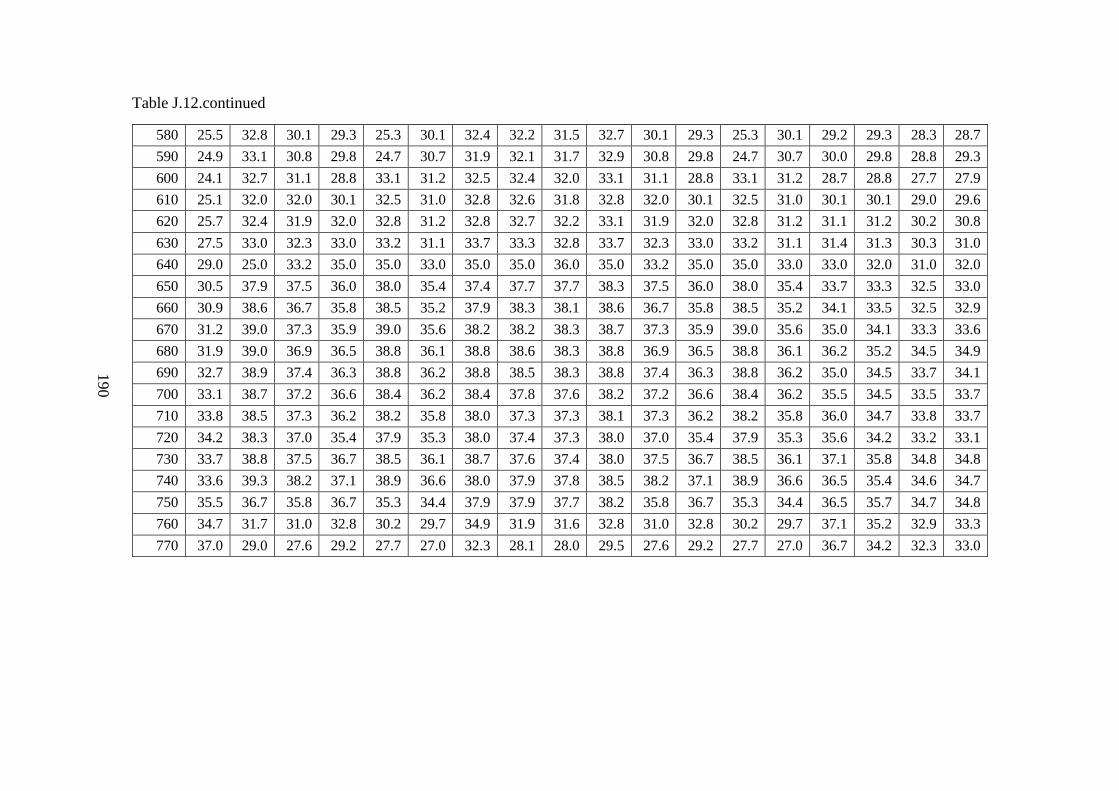
188


580 25.5 32.8 30.1 29.3 25.3 30.1 32.4 32.2 31.5 32.7 30.1 29.3 25.3 30.1 29.2 29.3 28.3 28.7

590 24.9 33.1 30.8 29.8 24.7 30.7 31.9 32.1 31.7 32.9 30.8 29.8 24.7 30.7 30.0 29.8 28.8 29.3

600 24.1 32.7 31.1 28.8 33.1 31.2 32.5 32.4 32.0 33.1 31.1 28.8 33.1 31.2 28.7 28.8 27.7 27.9

610 25.1 32.0 32.0 30.1 32.5 31.0 32.8 32.6 31.8 32.8 32.0 30.1 32.5 31.0 30.1 30.1 29.0 29.6

620 25.7 32.4 31.9 32.0 32.8 31.2 32.8 32.7 32.2 33.1 31.9 32.0 32.8 31.2 31.1 31.2 30.2 30.8

630 27.5 33.0 32.3 33.0 33.2 31.1 33.7 33.3 32.8 33.7 32.3 33.0 33.2 31.1 31.4 31.3 30.3 31.0

640 29.0 25.0 33.2 35.0 35.0 33.0 35.0 35.0 36.0 35.0 33.2 35.0 35.0 33.0 33.0 32.0 31.0 32.0

650 30.5 37.9 37.5 36.0 38.0 35.4 37.4 37.7 37.7 38.3 37.5 36.0 38.0 35.4 33.7 33.3 32.5 33.0

660 30.9 38.6 36.7 35.8 38.5 35.2 37.9 38.3 38.1 38.6 36.7 35.8 38.5 35.2 34.1 33.5 32.5 32.9

670 31.2 39.0 37.3 35.9 39.0 35.6 38.2 38.2 38.3 38.7 37.3 35.9 39.0 35.6 35.0 34.1 33.3 33.6

680 31.9 39.0 36.9 36.5 38.8 36.1 38.8 38.6 38.3 38.8 36.9 36.5 38.8 36.1 36.2 35.2 34.5 34.9

690 32.7 38.9 37.4 36.3 38.8 36.2 38.8 38.5 38.3 38.8 37.4 36.3 38.8 36.2 35.0 34.5 33.7 34.1

700 33.1 38.7 37.2 36.6 38.4 36.2 38.4 37.8 37.6 38.2 37.2 36.6 38.4 36.2 35.5 34.5 33.5 33.7

710 33.8 38.5 37.3 36.2 38.2 35.8 38.0 37.3 37.3 38.1 37.3 36.2 38.2 35.8 36.0 34.7 33.8 33.7

720 34.2 38.3 37.0 35.4 37.9 35.3 38.0 37.4 37.3 38.0 37.0 35.4 37.9 35.3 35.6 34.2 33.2 33.1

730 33.7 38.8 37.5 36.7 38.5 36.1 38.7 37.6 37.4 38.0 37.5 36.7 38.5 36.1 37.1 35.8 34.8 34.8

740 33.6 39.3 38.2 37.1 38.9 36.6 38.0 37.9 37.8 38.5 38.2 37.1 38.9 36.6 36.5 35.4 34.6 34.7

750 35.5 36.7 35.8 36.7 35.3 34.4 37.9 37.9 37.7 38.2 35.8 36.7 35.3 34.4 36.5 35.7 34.7 34.8

760 34.7 31.7 31.0 32.8 30.2 29.7 34.9 31.9 31.6 32.8 31.0 32.8 30.2 29.7 37.1 35.2 32.9 33.3

770 37.0 29.0 27.6 29.2 27.7 27.0 32.3 28.1 28.0 29.5 27.6 29.2 27.7 27.0 36.7 34.2 32.3 33.0

190

189


780 37.5 29.4 27.3 30.5 27.3 27.5 34.4 30.5 29.8 30.2 27.3 30.5 27.3 27.5 35.5 34.1 33.2 33.7

790 38.7 30.7 31.5 32.2 30.3 29.3 31.8 31.2 32.0 32.5 31.5 32.2 30.3 29.3 35.8 33.3 32.7 33.8

800 36.7 29.2 30.6 30.8 28.4 27.9 31.2 28.5 28.9 29.7 30.6 30.8 28.4 27.9 35.3 33.3 31.5 32.3

810 35.9 27.6 28.5 32.2 26.7 28.0 33.2 29.8 29.7 29.8 28.5 32.2 26.7 28.0 36.3 35.3 34.0 34.5

820 35.6 29.3 30.1 32.0 28.9 29.0 31.4 30.2 30.6 31.5 30.1 32.0 28.9 29.0 36.2 34.0 32.5 33.6

830 36.9 30.9 29.2 29.9 30.0 29.0 31.2 28.3 27.9 29.9 29.2 29.9 30.0 29.0 36.5 34.6 32.5 33.7

840 37.1 28.4 27.9 31.5 27.1 27.8 33.1 29.5 28.2 30.1 27.9 31.5 27.1 27.8 36.1 35.3 33.0 34.1

850 35.9 31.2 29.8 31.0 30.8 30.0 30.9 28.5 28.1 29.8 29.8 31.0 30.8 30.0 36.5 34.3 32.5 33.7

860 36.3 29.0 28.1 31.8 27.8 28.3 33.2 29.4 29.0 30.1 28.1 31.8 27.8 28.3 35.2 34.5 32.3 33.1

870 37.3 28.9 28.1 29.9 27.5 27.6 31.5 28.5 29.0 29.8 28.1 29.9 27.5 27.6 35.6 33.4 31.9 32.9

880 36.7 28.3 26.8 29.2 27.1 26.8 31.4 27.8 28.4 29.6 26.8 29.2 27.1 26.8 35.3 33.5 31.9 32.9

890 36.8 29.2 28.8 30.4 28.0 28.0 31.8 28.8 29.4 30.6 28.8 30.4 28.0 28.0 35.2 33.4 32.4 33.3

900 42.0 28.5 27.2 29.5 27.5 27.3 30.3 26.8 27.5 29.0 27.2 29.5 27.5 27.3 35.8 33.9 32.5 33.5

910 44.1 29.3 28.9 32.2 27.9 28.8 32.0 29.8 29.6 30.4 28.9 32.2 27.9 28.8 36.2 35.1 34.8 35.5

920 42.2 28.7 27.2 27.9 27.8 27.0 31.4 26.9 26.1 28.0 27.2 27.9 27.8 27.0 35.8 33.5 31.9 33.2

930 40.6 29.7 26.7 31.2 28.0 28.9 34.7 30.6 29.2 29.3 26.7 31.2 28.0 28.9 35.3 34.5 33.8 34.4

940 41.1 28.8 25.9 29.9 28.0 27.9 31.6 28.5 28.0 29.2 25.9 29.9 28.0 27.9 34.6 32.9 31.6 32.8

950 41.0 29.6 30.2 31.6 28.2 29.0 33.8 30.4 30.0 30.9 30.2 31.6 28.2 29.0 33.5 34.7 34.7 35.3

960 38.6 28.2 29.0 29.7 27.3 27.2 30.9 28.0 28.2 29.5 29.0 29.7 27.3 27.2 34.8 33.7 34.0 37.0

970 37.0 28.5 28.8 31.0 27.3 27.8 31.6 30.3 30.3 30.8 28.8 31.0 27.3 27.8 35.3 33.9 33.7 35.5

191

190


980 37.8 29.3 29.0 29.8 28.8 28.0 30.0 28.9 29.3 30.3 29.0 29.8 28.8 28.0 35.8 33.7 32.6 33.9

990 35.1 26.0 27.5 30.8 27.2 28.0 30.7 28.6 28.8 29.9 27.5 30.8 27.2 28.0 35.6 34.0 32.2 32.8

1000 36.2 25.2 26.4 29.8 24.4 25.4 29.2 27.4 27.7 28.7 26.4 29.8 24.4 25.4 35.9 33.8 32.3 33.3

1010 38.1 27.9 28.0 29.5 26.0 26.2 31.0 30.5 30.6 30.8 28.0 29.5 26.0 26.2 35.6 34.6 34.1 34.6

1020 37.8 30.7 29.4 28.1 29.5 27.8 28.6 28.2 29.0 30.4 29.4 28.1 29.5 27.8 35.6 33.4 32.2 33.1

1030 38.2 28.1 26.7 29.7 25.9 26.4 28.7 27.7 28.7 30.0 26.7 29.7 25.9 26.4 35.1 34.3 32.4 33.2

1040 35.7 31.8 30.3 31.3 31.2 30.3 26.6 29.2 31.1 32.3 30.3 31.3 31.2 30.3 34.5 32.7 32.3 33.3

1050 35.8 31.2 28.8 30.9 30.2 29.6 28.3 26.7 27.6 29.5 28.8 30.9 30.2 29.6 35.8 34.2 32.5 33.5

1060 36.0 28.1 26.8 31.1 27.1 27.9 29.8 27.8 27.8 28.9 26.8 31.1 27.1 27.9 33.7 33.4 32.2 32.8

1070 35.1 29.1 28.5 29.7 28.7 28.2 28.1 29.2 29.7 30.7 28.5 29.7 28.7 28.2 32.4 31.5 31.5 32.2

1080 35.0 30.5 29.3 28.7 30.0 28.5 27.3 27.3 28.9 30.5 29.3 28.7 30.0 28.5 32.9 31.3 30.2 31.2

1090 36.0 27.8 26.2 28.8 26.2 26.3 28.5 26.5 26.8 28.7 26.2 28.8 26.2 26.3 33.8 32.9 31.3 32.0

1100 34.7 32.2 31.0 30.0 31.7 29.7 30.2 30.8 31.0 32.1 31.0 30.0 31.7 29.7 32.8 32.1 31.7 32.3

1110 34.3 34.3 33.3 31.4 33.8 31.2 32.4 33.1 33.2 34.2 33.3 31.4 33.8 31.2 33.0 32.3 31.8 32.1

1120 34.8 35.7 34.9 32.2 35.2 32.0 33.7 34.3 34.4 35.2 34.9 32.2 35.2 32.0 33.5 32.9 32.4 32.6

1130 33.0 35.4 34.9 32.5 34.9 32.3 34.2 34.6 34.7 35.5 34.9 32.5 34.9 32.3 33.0 32.7 32.2 32.1

1140 32.7 34.9 35.9 33.0 34.6 32.7 34.0 34.2 34.2 34.8 35.9 33.0 34.6 32.7 32.5 32.4 32.0 31.9

1150 31.4 33.3 33.5 32.2 33.3 31.8 32.7 32.8 32.8 33.2 33.5 32.2 33.3 31.8 31.4 31.3 31.0 31.0

1160 31.0 32.2 33.7 31.4 32.1 31.1 31.5 31.7 31.6 32.0 33.7 31.4 32.1 31.1 30.6 30.5 30.3 30.2

1170 30.5 31.3 32.0 30.8 31.3 30.5 30.6 30.8 30.7 31.0 32.0 30.8 31.3 30.5 30.0 30.0 29.8 29.7

192

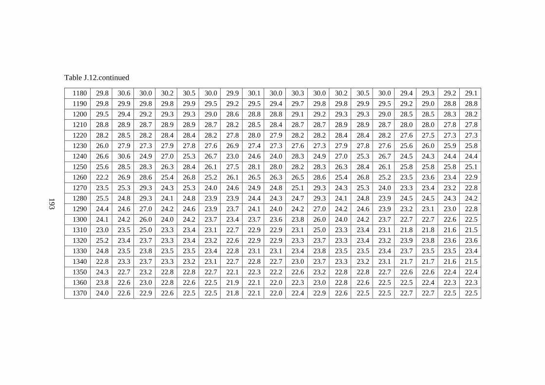
191


1180 29.8 30.6 30.0 30.2 30.5 30.0 29.9 30.1 30.0 30.3 30.0 30.2 30.5 30.0 29.4 29.3 29.2 29.1

1190 29.8 29.9 29.8 29.8 29.9 29.5 29.2 29.5 29.4 29.7 29.8 29.8 29.9 29.5 29.2 29.0 28.8 28.8

1200 29.5 29.4 29.2 29.3 29.3 29.0 28.6 28.8 28.8 29.1 29.2 29.3 29.3 29.0 28.5 28.5 28.3 28.2

1210 28.8 28.9 28.7 28.9 28.9 28.7 28.2 28.5 28.4 28.7 28.7 28.9 28.9 28.7 28.0 28.0 27.8 27.8

1220 28.2 28.5 28.2 28.4 28.4 28.2 27.8 28.0 27.9 28.2 28.2 28.4 28.4 28.2 27.6 27.5 27.3 27.3

1230 26.0 27.9 27.3 27.9 27.8 27.6 26.9 27.4 27.3 27.6 27.3 27.9 27.8 27.6 25.6 26.0 25.9 25.8

1240 26.6 30.6 24.9 27.0 25.3 26.7 23.0 24.6 24.0 28.3 24.9 27.0 25.3 26.7 24.5 24.3 24.4 24.4

1250 25.6 28.5 28.3 26.3 28.4 26.1 27.5 28.1 28.0 28.2 28.3 26.3 28.4 26.1 25.8 25.8 25.8 25.1

1260 22.2 26.9 28.6 25.4 26.8 25.2 26.1 26.5 26.3 26.5 28.6 25.4 26.8 25.2 23.5 23.6 23.4 22.9

1270 23.5 25.3 29.3 24.3 25.3 24.0 24.6 24.9 24.8 25.1 29.3 24.3 25.3 24.0 23.3 23.4 23.2 22.8

1280 25.5 24.8 29.3 24.1 24.8 23.9 23.9 24.4 24.3 24.7 29.3 24.1 24.8 23.9 24.5 24.5 24.3 24.2

1290 24.4 24.6 27.0 24.2 24.6 23.9 23.7 24.1 24.0 24.2 27.0 24.2 24.6 23.9 23.2 23.1 23.0 22.8

1300 24.1 24.2 26.0 24.0 24.2 23.7 23.4 23.7 23.6 23.8 26.0 24.0 24.2 23.7 22.7 22.7 22.6 22.5

1310 23.0 23.5 25.0 23.3 23.4 23.1 22.7 22.9 22.9 23.1 25.0 23.3 23.4 23.1 21.8 21.8 21.6 21.5

1320 25.2 23.4 23.7 23.3 23.4 23.2 22.6 22.9 22.9 23.3 23.7 23.3 23.4 23.2 23.9 23.8 23.6 23.6

1330 24.8 23.5 23.8 23.5 23.5 23.4 22.8 23.1 23.1 23.4 23.8 23.5 23.5 23.4 23.7 23.5 23.5 23.4

1340 22.8 23.3 23.7 23.3 23.2 23.1 22.7 22.8 22.7 23.0 23.7 23.3 23.2 23.1 21.7 21.7 21.6 21.5

1350 24.3 22.7 23.2 22.8 22.8 22.7 22.1 22.3 22.2 22.6 23.2 22.8 22.8 22.7 22.6 22.6 22.4 22.4

1360 23.8 22.6 23.0 22.8 22.6 22.5 21.9 22.1 22.0 22.3 23.0 22.8 22.6 22.5 22.5 22.4 22.3 22.3

1370 24.0 22.6 22.9 22.6 22.5 22.5 21.8 22.1 22.0 22.4 22.9 22.6 22.5 22.5 22.7 22.7 22.5 22.5

193

192


1380 23.2 22.5 22.8 22.7 22.5 22.4 21.8 22.0 22.0 22.3 22.8 22.7 22.5 22.4 21.7 21.7 21.5 21.5

1390 23.8 22.5 22.8 22.6 22.5 22.5 21.7 22.0 22.0 22.3 22.8 22.6 22.5 22.5 22.4 22.3 22.2 22.2

1400 24.0 22.5 22.9 22.7 22.5 22.5 21.8 22.1 22.0 22.4 22.9 22.7 22.5 22.5 22.5 22.4 22.3 22.3

1410 23.8 22.6 23.0 22.8 22.6 22.6 21.9 22.2 22.2 22.5 23.0 22.8 22.6 22.6 22.5 22.4 22.2 22.3

1420 23.8 22.7 23.1 22.9 22.7 22.7 21.9 22.2 22.2 22.5 23.1 22.9 22.7 22.7 22.5 22.4 22.3 22.3

1430 23.9 22.6 23.0 22.8 22.5 22.6 21.9 22.1 22.1 22.5 23.0 22.8 22.5 22.6 22.6 22.6 22.4 22.4

1440 24.0 22.6 22.9 22.8 22.6 22.6 21.9 22.1 22.1 22.4 22.9 22.8 22.6 22.6 22.5 22.5 22.3 22.3

194

193

APPENDIX K

SAMPLE CALCULATION

K.1 Sample Calculation for Productivity

A sample calculation for the productivity for RUN 072015-R1 on July 16, 2015 was shown

below. The total gas produced was 556 mL, and the hydrogen percentage was 95.8%. Day time

was 14 hours. The volume of Reactor 1 (R1) was 11 L.

𝑉𝐻2 = (556 𝑚𝐿) ∙ (0.958) = 532 𝑚𝐿 (𝐾. 1)

𝑛𝐻2 =𝑃𝑉𝐻2

𝑅𝑇 (𝐾. 2)

𝑛𝐻2 =(0.9 𝑏𝑎𝑟)(532 𝑚𝐿)

(85.14 𝑏𝑎𝑟. 𝑚𝐿𝑚𝑜𝑙. 𝐾

) (303𝐾)= 0.019 𝑚𝑜𝑙 (𝐾. 3)

Recall

𝑃𝑟𝑜𝑑𝑢𝑐𝑡𝑖𝑣𝑖𝑡𝑦 =𝐻𝑦𝑑𝑟𝑜𝑔𝑒𝑛 𝑝𝑟𝑜𝑑𝑢𝑐𝑒𝑑

𝑅𝑒𝑎𝑐𝑡𝑜𝑟 𝑉𝑜𝑙𝑢𝑚𝑒 ∙ 𝑇𝑖𝑚𝑒 (2.7)

𝑃𝑟𝑜𝑑𝑢𝑐𝑡𝑖𝑣𝑖𝑡𝑦 =0.019 𝑚𝑜𝑙

(0.011 𝑚3) ∙ (14 ℎ) (𝐾. 4)

𝑃𝑟𝑜𝑑𝑢𝑐𝑡𝑖𝑣𝑖𝑡𝑦 = 0.123𝑚𝑜𝑙

(𝑚3. ℎ) (𝐾. 5)

194

K.2 Sample Calculation for Substrate Conversion Efficiency

A sample calculation for the substrate conversion efficiency (YH2) for RUN 072015-R1 on July

16, 2015 was performed below. On July 16, 2015 in the morning, acetic acid concentration in

the reactor was adjusted to 40 mM (0.440 mol). Acetic acid measured in the morning on July

17, 2015 before feeding was 36.54 mM (0.402 mol). Hydrogen produced on July 16, 2015 was

0.019 mol as calculated previously.

Recall:

𝑌𝐻2 =𝐻𝑦𝑑𝑜𝑟𝑔𝑒𝑛 𝑝𝑟𝑜𝑑𝑢𝑐𝑒𝑑

𝑇ℎ𝑒𝑜𝑟𝑒𝑡𝑖𝑐𝑎𝑙 ℎ𝑦𝑑𝑟𝑜𝑔𝑒𝑛 𝑡ℎ𝑎𝑡 𝑐𝑜𝑢𝑙𝑑 𝑏𝑒 𝑝𝑟𝑜𝑑𝑢𝑐𝑒𝑑 𝑖𝑓 𝑎𝑙𝑙 𝑡ℎ𝑒 𝑠𝑢𝑏𝑠𝑡𝑟𝑎𝑡𝑒 𝑤𝑎𝑠 𝑢𝑠𝑒𝑑 𝑓𝑜𝑟 𝐻2 𝑝𝑟𝑜𝑑𝑢𝑐𝑡𝑖𝑜𝑛

𝑥100 (2.6)

Theoretically, 4 mol of hydrogen can be produced from 1 mol of acetic acid (see Reaction 2.16).

𝑌𝐻2 =0.019 𝑚𝑜𝑙

(0.440 𝑚𝑜𝑙 − 0.402 𝑚𝑜𝑙) ∙ 4∙ 100 = 12.5 % (𝐾. 6)

Substrate conversion efficiency for RUN 072015-R2 was calculated in the same way. Since

sucrose is the substrate, theoretically, 24 mol of hydrogen can be produced from 1 mol of

sucrose (Reaction 2.17). Therefore, while calculating the theoretical hydrogen production,

sucrose consumption was multiplied with 24 instead of 4.

K.3 Sample Calculation for Light Conversion Efficiency

A sample calculation for the light conversion efficiency for RUN 072015-R1 on July 16, 2015

was shown below. The daily solar radiation was 322.20 W/m2. Hydrogen density was 0.0899

kg/m3 (8.99x10-5 g/mL). The irradiated area was calculated as 1.685 m2.

195

Recall:

𝜂 =𝑉𝐻2 ∙ 𝜌𝐻2 ∙ 33.61

𝐼 ∙ 𝐴 ∙ 𝑡𝐻2∙ 100 (2.8)

𝜂 =(532 𝑚𝐿) ∙ (8.99 ∙ 10−5 𝑔/𝑚𝐿) ∙ (33.61

𝑊. ℎ𝑔 )

(526.46𝑊𝑚2) ∙ (1.685 𝑚2) ∙ (14 ℎ)

∙ 100 = 0.01295 % (𝐾. 7)

DESIGN AND ANALYSIS OF TUBULAR …etd.lib.metu.edu.tr/upload/12619241/index.pdfI hereby declare that...

Documents

Transcript of DESIGN AND ANALYSIS OF TUBULAR …etd.lib.metu.edu.tr/upload/12619241/index.pdfI hereby declare that...